Forecasting the volatility of EUA futures with economic policy uncertainty using the GARCH‑MIDAS modelJian Liu1, Ziting Zhang1, Lizhao Yan2 and Fenghua Wen3*

IntroductionSince the inception of the European Union Emissions Trading System (EU ETS), carbon derivatives have been traded. Moreover, futures trading is the main section of the EU ETS. Carbon futures not only provides more effective risk management tools for enter-prises controlling emissions but also opportunities for investors to engage in speculative arbitrage activities. Hence, carbon futures help improve market liquidity and effectively circumvent the risk for participants (Zhou and Li 2019). Moreover, the price fluctuations of carbon futures can reflect overall market price trend (Tang et  al. 2013; Milunovich and Joyeux 2010). This provides a basis for carbon market policymakers to formulate effective management policies. Owing to the relatively short development history, the risk mechanism for the EU carbon market has not yet been completed. An effective method of volatility forecasting can contribute to improving risk management capabil-ity. Meanwhile, increasing participation of financial intermediaries and international

Abstract

This study investigates the impact of economic policy uncertainty (EPU) on the volatility of European Union (EU) carbon futures prices and whether it has predictive power for the volatility of carbon futures prices. The GARCH-MIDAS model is applied for evaluating the impact of different EPU indexes on the price volatility of European Union Allowance (EUA) futures. We then compare the predictive power for the volatility of the two GARCH-MIDAS models based on different EPU indexes and six GARCH-type models. Our empirical results show that the GARCH-MIDAS models, which exhibit superior out-of-sample predictive ability, outperform GARCH-type models. The results also indicate that EPU has noticeable effect on the volatility of EUA futures. Specifically, the forecast accuracy of the EU EPU index is significantly higher than that of the global EPU index. Robustness checks further confirm that the EPU index (especially the EPU index of the EU) has strong predictive power for EUA futures prices. Additionally, using the volatility forecasting methods that GARCH-MIDAS models combine with the EPU index, investors can construct their portfolios to realize economic returns.

Keywords: EUA, Economic policy uncertainty, GARCH-MIDAS, Volatility forecasting, Futures

Open Access

© The Author(s), 2021. Open Access This article is licensed under a Creative Commons Attribution 4.0 International License, which permits use, sharing, adaptation, distribution and reproduction in any medium or format, as long as you give appropriate credit to the original author(s) and the source, provide a link to the Creative Commons licence, and indicate if changes were made. The images or other third party material in this article are included in the article’s Creative Commons licence, unless indicated otherwise in a credit line to the mate-rial. If material is not included in the article’s Creative Commons licence and your intended use is not permitted by statutory regulation or exceeds the permitted use, you will need to obtain permission directly from the copyright holder. To view a copy of this licence, visit http:// creat iveco mmons. org/ licen ses/ by/4. 0/.

RESEARCH

Liu et al. Financ Innov (2021) 7:76 https://doi.org/10.1186/s40854‑021‑00292‑8 Financial Innovation

*Correspondence: mailtowfh@126.com 3 Business School, Central South Univerdity, Changsha, Hunan, People’s Republic of ChinaFull list of author information is available at the end of the article

Page 2 of 19Liu et al. Financ Innov (2021) 7:76

economics and politics has increased the complexity and volatility of the carbon market. For these reasons, effective measurement of carbon futures market volatility is of great significance for market participants. Therefore, predictions on EU ETS carbon futures price volatility were analyzed.

Currently, economic situations and policy adjustments have proven vital in the volatil-ity of carbon prices (Zhu and Chevallier 2017; Kautto et al. 2012; Fan et al. 2017; Cheval-lier 2011). Economic and policy changes also signify uncertainty. From the perspective of the underlying logic of the relationship, the uncertainty caused by economic policy changes mainly affects the carbon futures market through the following three channels. First, since the generation and operation of the carbon futures market primarily depend on government policies, the allocation system will directly determine the supply of the carbon quota in the market. This affects the price of carbon futures (Chevallier 2009; Kanamura 2019; Mansanet-Bataller and Pardo 2009). Second, the uncertainty regarding economic policy changes will affect the production behavior and carbon emissions of regulated enterprises, which affects the demand for the carbon quota and causing price fluctuations in carbon futures. Alshubiri et al. (2020) highlight that the 2008 subprime mortgage reduced the activities of oil-relevant enterprises, and Bel and Joseph (2015) found that the economic recession caused by the subprime mortgage crisis in 2008 led to a sharp decrease in the demand for carbon quota and caused the carbon quota price to plummet. Third, economic policy uncertainty will have an impact on the energy market (Wei et al. 2017; Aloui et al. 2016; Yin 2016; Chen et al. 2020). In contrast, volatility in the energy market can affect the carbon futures market (Chevallier 2011; Mansanet-Bataller et  al. 2007; Dutta 2019; Liu and Chen 2013). First, economic and policy factors influ-ence the price of non-clean energy, which affects the production behavior of enterprises. Moreover, this further changes the carbon quota demand, leading to fluctuations in car-bon futures prices. In contrast, supported by advances in clean energy technologies and environmental policies, enterprises may apply clean energy to replace non-clean energy. Moreover, energy consumption is related to carbon dioxide emissions(Khan et al. 2020). Here, carbon dioxide emissions per unit of capacity are reduced, resulting in decreased demand for carbon quotas and lower carbon price. Therefore, economic policy uncer-tainty has certain explanatory power for fluctuations in the carbon futures market.

The existing literature quantitatively measures economic policy uncertainty. Baker et  al. (2016) proposed economic policy uncertainty (EPU) index for the major econo-mies of the world. The EPU is based on the frequency of keywords, such as uncertainty, economic activity, and policy adjustments, found in newspaper coverage. The global EPU (GEPU) index is measured by Davis (2016), which is obtained by the GDP-weighted average of the EPU index of 20 countries accounting for two-thirds of the total global output. Since its introduction, the EPU index has been extensively applied in research. Moreover, based on our analysis of the relationship between EPU and the volatility of the carbon futures market, introducing EPU to explore its explanatory and predictive ability for the EUA futures fluctuations is appropriate.

This study adopts the GARCH mixed frequency data sampling (GARCH-MIDAS) model proposed by Engle et al. (2013), which allows data of different frequencies to be incorporated into the same model. Moreover, it decomposes the variance into long-term and short-term components, which can effectively enhance the prediction accuracy.

Page 3 of 19Liu et al. Financ Innov (2021) 7:76

Therefore, the GARCH-MIDAS model is adopted to explore the connection between EPU and EUA futures. Additionally, the GARCH-MIDAS model and GARCH-type models are compared in terms of predictive performance for EUA futures.

Our analysis of the relationship between the EU carbon futures market and economic policy uncertainty is original and can provide a new perspective for measuring the vola-tility of the EU carbon futures market. The main contributions of this study can be sum-marized as follows. First, combined with the GARCH-MIDAS model proposed by Engle et al. (2013), we add the EPU index to the EUA futures forecasting model. The empiri-cal results confirm that the EPU has great predictive performance for the volatility of EUA futures and that GARCH-MIDAS models significantly outperform GARCH-type models in forecasting performance by using the out-of-sample test. Our analysis proves that EPU is a new and valid approach to EUA futures volatility forecasts. Second, we not only investigate the influence of GEPU on EUA futures volatility and its prediction performance but also introduce the EEPU to analyze and predict EUA futures volatil-ity. By comparing their predictive ability, we verified that EEPU can be more effective in predicting carbon futures price volatility than GEPU. Third, by constructing a portfolio of EUA futures and risk-free EU rates, our method can produce the economic value of volatility forecasting in practical applications.

The remainder of this paper is organized as follows. "Related literature" section pre-sents the related literature. "Model and methodology” section describes the method-ology of the study. "Data and statistical description" section  introduces the data and its characteristics. “Empirical analysis” section  presents the empirical analysis. Finally, “Conclusions” section.  concludes the paper.

Related literatureEffective measurement of carbon futures market volatility is of great significance for var-ious participants in the EU ETS carbon futures market. Currently, economic conditions and policy adjustments have proved vital factors in the volatility of carbon prices. An increasing number of studies have explored the links between carbon prices and macro-economic information. Chevallier (2011) highlighted that the carbon market is affected during periods of economic expansion (recession). This confirms the existence of a link between the macroeconomic conditions and carbon price. Zhu and Chevallier (2017) confirmed that a long-term co-integration relationship exists between carbon prices and drivers, such as economic activities. The connection between carbon prices and policy changes has also been explored (Kautto et al. 2012; Fan et al. 2017). Kautto et al. (2012)verified the mutual influence between climate policy and carbon emission right price through their research. Fan et al. (2017) found that the adjustment of regulatory policies in EU ETS would also affect the earnings of European Union Allowance (EUA). Com-bined, these studies indicate that carbon prices are strongly tied to economic situations and policy changes.

Economic and policy changes also signify uncertainty. Existing literature quantitatively measures economic policy uncertainty. Since its introduction, the EPU index has been extensively applied in research. In the stock market volatility prediction, many studies show that the EPU index has significant and positive impact on both the Chinese stock market and that of the United States (Balcilar et al. 2019; Bahmani-Oskooee and Saha

Page 4 of 19Liu et al. Financ Innov (2021) 7:76

2019; Li et al. 2019; Yu and Song 2018; Hoque and Zaidi 2019). Regarding the volatility forecast in the energy market, some studies have proved that the EPU is significantly related to the energy market price and has superior predictive effects in out-of-sample tests (Wei et al. 2017; Aloui et al. 2016; Yin 2016). Additionally, Fang et al. (2018) hold that the GEPU index has remarkable predictive ability regarding the volatility of the global gold futures market. Some scholars have also confirmed that the EPU has note-worthy impacts on markets such as virtual currencies and correlations between various markets (Fang et al. 2017, 2019). Additionally, EPU can also affect the company’s deci-sion-making behavior, such as the financial asset allocation of a company (Huang et al. 2019; Wen et al. 2019; Yan et al. 2019) and cash flow holding (Li 2019). Based on our analysis of the relationship between EPU and the volatility of the carbon futures market above, EPU may have a certain explanatory power on carbon futures price fluctuations and can be used to predict price fluctuations in the carbon market. In addition to the influence of the economic policy in the EU, the market volatility of EUA futures may also be affected by other large economic policy changes. Therefore, we introduce the EU EPU (EEPU) and GEPU index to explore the explanatory ability of EUA futures and its ability to predict long-term fluctuations, respectively.

Existing studies mainly use classic financial time-series prediction methods, such as ARCH and GARCH-type models, to forecast the price of carbon financial prod-ucts (Emenogu et al. 2020; Challa et al. 2018; Dhamija et al. 2017; Byun and Cho 2013; Koop and Tole 2013; Zeitlberger and Brauneis 2016; Venmans 2015). Nevertheless, these methods cannot guarantee both long-term and short-term prediction accuracy (Lei et al. 2018). When exogenous variables of different frequencies are added, only fre-quency reduction can be adopted. The processing method of frequency reduction will lose effective information from the high-frequency data and may lead to a decline in the prediction accuracy. An extended form of the model can meet more research needs (Zha et al. 2020). In this case, the GARCH-MIDAS model can effectively enhance the forecast accuracy by simultaneously incorporating the data of different frequencies simultane-ously. Since its introduction, many scholars have used the GARCH-MIDAS model to analyze the volatility of the stock and energy markets, and they confirmed that the model has superior predictive performance (Yu et al. 2018; Fang et al. 2017; Wei et al. 2017; Lei et al. 2018; Li et al. 2019). The GARCH-MIDAS model has become essential for research on the correlation between macroeconomic factors and market fluctuations. Similar to general financial markets, the price volatility of EUA futures has a significant GARCH effect (Byun and Cho 2013). Hence, applying the GARCH-MIDAS model to the EU car-bon market is reasonable. Therefore, we use the GARCH-MIDAS model combined with EPU to analyze and predict fluctuations in EUA futures prices. The results show that the GARCH-MIDAS model exceeds the GARCH-type models relative to predictive perfor-mance. This provides new insights into modeling and forecasting carbon price volatility.

Model and methodologyGARCH‑MIDAS model

To explore the contribution of a monthly frequency EPU index to the long-term volatility of daily frequency EUA futures, we adopt the GARCH-MIDAS model proposed by Engle et al. (2013). Unlike GARCH-type models, the variance is decomposed into long-term

Page 5 of 19Liu et al. Financ Innov (2021) 7:76

and short-term volatility components. Short-term fluctuations remain determined by historical fluctuation information. In contrast, long-term fluctuations are characterized by low-frequency macroeconomic variables. The basic forms are as follows:

where ri,t refers to the log return of financial assets on day i of month t, and µ is the non-conditional mean of the return sequence. The term Nt denotes the number of days in a month. εi,t |�i−1,t ∼ N (0, 1) , given the information set �i−1,t up to day (i − 1) of period t. The conditional variance of the daily return is divided into two components: a short-run component defined as si,t and a long-run component defined as lt and σ 2

i,t is defined as the total conditional variance. The short-run volatility component si,t follows the tradi-tional GARCH (1,1) process as follows:

where α and β are the parameters to be estimated for the ARCH and GARCH compo-nents, respectively, where α > 0 , β > 0 , and α + β < 1 . Because the growth rate of the EPU index presented by Xt−k can have a negative value, according to Engle et al. (2013), we convert the long-term fluctuations into the logarithmic form in this study. This can be expressed as follows:

where m is an intercept and θ is the slope of the weighted effect of the low-frequency macroeconomic variables lagged behind the long-term volatility of financial asset returns. The term K denotes the maximum lag order of smooth volatility in MIDAS filtering. The marginal effect depends on θ and ω (Conrad et  al. 2014). In contrast, ϕk(ω1,ω2) represents the weighting scheme of beta weights with the independent vari-ables ω1 and ω2 , which can be expressed as follows:

Equation  5 is the unrestrictive weighting scheme that can produce attenuated and hump weight distributions. In contrast, Eq. 6 can be obtained from Eq. 5 with a con-straint of ω1 = 1 . The constraint of ω1 = 1 is applied to the unrestricted weight func-tion to obtain the restricted weight function Eq. 6. The restricted weighting function can only generate an attenuated weight distribution, and the attenuation rate is determined

(1)ri,t = µ+√

lt si,tεi,t , ∀i = 1, . . . ,Nt ,

(2)σ 2i,t = lt si,t ,

(3)si,t = (1− α − β)+ α(ri−1,t − µ)2

lt+ βsi−1,t ,

(4)log(lt) = m+ θ

K∑

k=1

ϕk(ω1,ω2)Xt−k ,

(5)ϕk(ω1,ω2) =(k/K )ω1−1(1− k/K )ω2−1

∑Kj=1(j/K )ω1−1(1− j/K )ω2−1

,

(6)ϕk(1,ω2) =(1− k/K )ω2−1

∑Kj=1(1− j/K )ω2−1

,

Page 6 of 19Liu et al. Financ Innov (2021) 7:76

by the parameters ω2 . This means that the larger the value of ω2 , the faster the decay rate, and vice versa. Both of these beta weighting functions can be applied to the estima-tion of the GARCH-MIDAS model. Following Conrad and Loch (2015), the restricted weight function of ω1 = 1 is selected. Equations 1, 3, 4, and 6 form a GARCH-MIDAS model based on the EPU exponential change rate. Additionally, quasi-maximum likeli-hood estimation (QMLE) was adopted to estimate the parameters and parameter space � = {µ,α,β ,m, θ ,ω}.

Regression‑based test for the specification of one‑component GARCH

According to Conrad and Schienle (2020), there should be misspecification testing in GARCH models in the sense of an omitted multiplicative long-term component. Hence, we apply the regression-based test proposed by Conrad and Schienle (2020) as a preliminary check before estimating the GARCH-MIDAS model. The regression model is considered in logarithmic form:

where Xt denotes the monthly explanatory variables, vt meets the independent identical distribution, and σ̂ 2

i,t is the estimated variance from the model under the null hypothesis of a simple GARCH. ri,t refers to the daily log returns. We define RV t as the sum of the volatility-adjusted squared daily returns within each month. The regression-based test checks whether the H0 : w0 = 0 that the one-component GARCH is correctly specified can be rejected when using EPU as an explanatory variable.

MCS test

To assess the predictive power of the volatility forecasts from the GARCH-MIDAS and GARCH-type models, various loss functions were used to compare the accuracies of the different models. More criteria make a more effective analysis (Kou et al. 2021). According to Hansen et al. (2011), we employ six loss functions as criteria for evaluating the prediction accuracy of various volatility models in the empirical examination. The specific definitions of these six types of loss functions are as follows:

(7)ln(RV t) = c + w0X0 + vt ,

(8)RV t =

M∑

i=1

r2i,t/σ̂2i,t ,

(9)MAE =1

T

T∑

i=1

|σ 2i − σ̂ 2

i |,

(10)MSE =1

T

T∑

i=1

(σ 2i − σ̂ 2

i )2,

(11)MAD =1

T

T∑

i=1

|σi − σ̂i|,

Page 7 of 19Liu et al. Financ Innov (2021) 7:76

where σ̂ 2i denotes the predicted value of the variance on day i obtained by the different

models, and σ 2i is the daily actual variance. The daily frequency realized variance is a

perfect proxy for the true conditional variance (Patton 2011). Nevertheless, owing to the unavailability of data, we use the square value of the daily real return to represent the daily actual fluctuation value (Wei et  al. 2017). Moreover, T represents the size of the out-of-sample prediction window.

However, the loss function could not distinguish whether the loss differences of the dif-ferent models were statistically significant. After the loss function value is obtained, we employ the model confidence set (MCS) test proposed by Hansen et al. (2011) to compare the prediction accuracy between models. The MCS test has an advantage over the conven-tional test model as it does not have to set a benchmark model. Moreover, it allows for the possibility of multiple optimal models. The MCS test process was expressed as follows:

First, it sets a model collection M0 , which contains m volatility forecasting models to be inspected. After calculating the loss values of the out-of-sample forecast, we write them as Liu,t for model u of the loss function i (out-of-sample window t = 1, . . . , n ). Therefore, for any two predictive volatility models in model collection M0 , the relative loss function val-ues are denoted as duv,t = Liu,t − Liv,t(u, v ∈ M0) . The superior object set is defined as M∗ , which can be expressed as follows:

where E(diuv,t) represents the mathematical expectation of duv,t under the specific loss function i . The MCS test is a series of continuous significance tests for the models of M0 , and the model that proves to be significantly inferior to the others is eliminated. The null hypothesis of the MCS test is as follows:

As shown above, the null hypothesis assumes that any two models have the same predic-tive power. The MCS test is conducted through a series of continuous significance tests wherein models of M0 with poor predictive power are eliminated until no models are excluded from M0 . Setting the confidence level α , if the p value is larger than α , this indi-cates that this model possesses superior out-of-sample predictive ability and can survive the MCS test. The larger the p value of the MCS test, the higher the prediction accu-racy of the corresponding model. Additionally, if the p value is smaller than α , then this

(12)MSD =1

T

T∑

i=1

(σi − σ̂i)2,

(13)QLIKE =1

T

T∑

i=1

(log(σ̂ 2i )+ σ 2

i /σ̂2i ),

(14)R2LOG =1

T

T∑

i=1

(log(σ 2i /σ̂

2i ))

2,

(15)M∗ ≡ {u ∈ M0 : E(diuv,t) ≤ 0 for all v ∈ M0},

(16)H0,M : E(diuv,t) ≤ 0 for all v ∈ M0

Page 8 of 19Liu et al. Financ Innov (2021) 7:76

volatility prediction model is proven to have poor out-of-sample predictive ability and will be removed from the MCS test.

Additionally, Hansen et  al. (2011) recommend using semi-quadratic statistics TSQ and range statistics TR in the model assessment process. These statistics are defined as follows:

If the p values of the TSQ and TR statistics are larger than the given confidence level α , then H0 , that is, the null hypothesis, cannot be rejected. Because the asymptotic distri-bution of the statistics TSQ and TR depends on the “aversion parameter” their real distri-butions are extraordinarily complicated. However, the bootstrap method can solve this difficulty and easily obtain the statistics TSQ , TR , and the corresponding pvalues.

Data and statistical descriptionThe data samples used in this study were divided into two parts. One part is the daily data of the consecutive settlement price of EUA futures from the European Climate Exchange, which is the most active carbon futures trading market in the world and includes mainly EUA futures. The other is the EPU index, which represents monthly data on macroeconomic variables. As the carbon quotas of phase I of the EU ETS are allocated for free, the enterprises controlling their emissions do not participate in car-bon market transactions. To ensure the adequacy and validity of the data, we use the data of phases II and III of the EU ETS. The EUA futures data cover the period from January 1, 2008, to September 30, 2019, including 3023 pieces of daily data from the WIND database. The EPU sample period spans from January 2008 to September 2019, with 141 pieces of monthly data (EPU data are available on http:// www. polic yunce rtain ty. com). According to Fang et al. (2017) and Liu et al. (2019a), we adopt the logarithmic rate of the returns for the EUA futures settlement price to narrow the value range of the variables so the returns of the EUA futures and EPU are of the same order of magni-tude. The transformed yield is expressed as R , and the growth rates of the EPU indexes are denoted as �GEPU and �EEPU , where �GEPU = (GEPUt − GEPUt−1)/GEPUt−1 , �EEPU = (EEPUt − EEPUt−1)/EEPUt−1 . The summary statistics of the transformed data are presented in Table 1.

As shown in Table 1, first, the SD of the EUA futures yield is much larger than its mean. This indicates that the EUA futures price exhibits certain volatility. Second, the yield of the EUA futures is obviously to the left and turns to form a sharp peak and thick tail. In contrast, the GEPU and EEPU indexes are to the right and have sharp

(17)TSQ = maxu,v∈M0

(di

uv)2

√var(diuv)

,

(18)TR = maxu,v∈M0

|di

uv|√var(diuv)

,

(19)di

uv =1

n

n∑

t=1

diuv ,

Page 9 of 19Liu et al. Financ Innov (2021) 7:76

peaks. The JB test also revealed that all yield (growth rate) sequences were signifi-cantly abnormally distributed and provided evidence of autocorrelation characteris-tics with different degrees. Finally, all results of the ADF test support the rejection of the null hypothesis of a unit root significantly. This implies that the all-time series is stationary and can thus be modeled. Furthermore, the variation trend diagrams of the EUA yield sequence, GEPU, and EEPU volatility sequences are shown in Fig. 1.

As displayed in Fig. 1, the four major events throughout the sample period result in significant fluctuations and an agglomeration effect of carbon futures prices. For instance, affected by the subprime mortgage crisis in 2008, companies were selling their excess carbon allowances, leading to a glut of carbon allowances in the market and plummeting of carbon prices. During the European debt crisis in 2011, GEPU and EEPU fluctuated drastically. The European economy was in recession, thus affecting carbon prices. EUA futures prices fluctuated sharply in 2013 as the EU ETS entered phase III because of the oversupply of carbon quotas in the first few months and the subsequent rejection of a ”volume auction” by the European parliament. Sub-sequently, structural reforms in the EU ETS led to an increase in prices. Additionally, the Brexit referendum in 2016, together with the presidential election of the USA and the interest rate of Fed raised, brought higher uncertainty to the global economy and increased volatility in EUA futures prices. Both the EPU index and EUA futures prices

Table 1 Descriptive statistics of transformed data

SD, standard deviation; Skew, skewness; Kurt, kurtosis; JB, Jarque‑Bera test; Ljung‑Box Q test of lagged 5 order (Q(5)); ADF, augmented Dickey‑Fuller unit root test. In the case of the ARCH test, the table reports the coefficient of a first‑order lag

***, **, *Indicate significance at the 1%, 5%, 10% levels, respectively

Variables Mean SD Skew Kurt JB Q(5) ADF ARCH test

R 0.3e−04 0.032 − 0.805 19.418 64.057*** 12.477** − 47.765*** 0.282***�GEPU 0.031 0.220 1.094 5.383 61.510*** 9.645* − 4.106 *** − 0.051**

�EEPU 0.030 0.233 1.238 6.578 111.300*** 12.120 ** − 4.524 *** − 0.040

Fig. 1 Time evolution of EUA return and growth rates of GEPU and EEPU

Page 10 of 19Liu et al. Financ Innov (2021) 7:76

fluctuated sharply during these four events. The price fluctuations of the EU carbon futures market can be considered closely related to economy and policy uncertainty.

Empirical analysisIn this section, we first conduct a regression-based test to check whether a simple GARCH is misspecified in the sense of an omitted long-term component. Second, we analyze the results of the parameter estimation of the two GARCH-MIDAS models based on different EPU indexes for the entire sample period. The data were then divided into two parts for the out-of-sample prediction of the rolling window.

Regression‑based test

As Table 2 shows, the results of parameter w0 are positive at the 1% significance level, indicating the connection between EPU and monthly realized volatility of EUA futures. Additionally, the results indicate that the two models are significant under the F-statistic test. Moreover, this means that in the null hypothesis, the one-component GARCH is correctly specified can be rejected. A significant relationship is found between the EPU index and the log of the volatility-adjusted realized variance of EUA futures. Therefore, this preliminary check can provide evidence that we can adopt the GARCH-MIDAS model to forecast EUA futures using the EPU index.

Model estimation

To examine the applicability of the GARCH-MIDAS model for the prediction of EUA futures volatility and analyze the influence of different EPU indexes, we perform a parameter estimation of the entire sample in this subsection. According to Conrad et al. (2015), the maximum lag order K of the model is determined using the information cri-terion. However, owing to the existence of a flexible weight function, a lag order that is as large as possible can be selected. After calculating the beta function with different lag orders, we choose 24 to be K . Hence, the lag time range of the influence of the EPU index on the volatility of the carbon futures market is 24 months. The parameter estima-tion results are presented in Table  3. First, the parameters µ , α , and β are significant, with the sum of α and β being close to 1. This indicates that the short-term volatility components of the EUA futures price yield show a noteworthy GARCH (1,1) effect. Sec-ond, both the estimated results of θ of these two models are positive at the 1% level, with the effect of GEPU being larger than that of EEPU. This implies that GEPU and EEPU are positively correlated with the long-term volatility components of the EUA futures yield and produce a positive effect on the EUA futures price. Basically, a larger growth

Table 2 Results of regression-based test

***, **, *Indicate significance at the 1%, 5%, 10% levels, respectively. The values in parentheses are the p values

Xt c w0 F-statistic

�GEPU 2.947*** 0.532*** 9.71***

(0.000) (0.002) (0.002)�

EEPU 2.945*** 0.561*** 12.890***

(0.000) (0.000) (0.001)

Page 11 of 19Liu et al. Financ Innov (2021) 7:76

rate of the EPU index leads to higher volatility in the EUA futures price. Overall, the GEPU and EEPU indexes have significant and positive effects on the long-term com-ponents of the EU carbon futures market volatility. When economic policy uncertainty increases, the EU carbon market becomes more volatile. Once the economic cycle of a recession is entered, the economic activity of factories will be greatly reduced. Therefore, the demand for quotas will be greatly reduced, resulting in drastic fluctuations in carbon prices in the carbon market. Market participants in the EU carbon market should be vigilant during periods of high economic policy uncertainty.

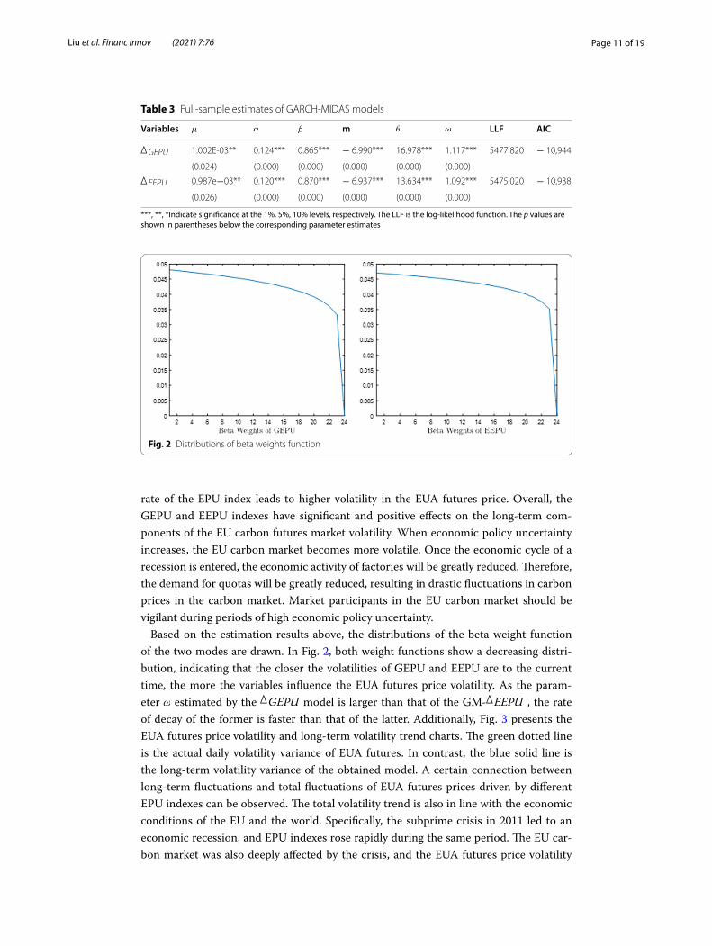
Based on the estimation results above, the distributions of the beta weight function of the two modes are drawn. In Fig. 2, both weight functions show a decreasing distri-bution, indicating that the closer the volatilities of GEPU and EEPU are to the current time, the more the variables influence the EUA futures price volatility. As the param-eter ω estimated by the

�

GEPU model is larger than that of the GM-�

EEPU , the rate of decay of the former is faster than that of the latter. Additionally, Fig. 3 presents the EUA futures price volatility and long-term volatility trend charts. The green dotted line is the actual daily volatility variance of EUA futures. In contrast, the blue solid line is the long-term volatility variance of the obtained model. A certain connection between long-term fluctuations and total fluctuations of EUA futures prices driven by different EPU indexes can be observed. The total volatility trend is also in line with the economic conditions of the EU and the world. Specifically, the subprime crisis in 2011 led to an economic recession, and EPU indexes rose rapidly during the same period. The EU car-bon market was also deeply affected by the crisis, and the EUA futures price volatility

Table 3 Full-sample estimates of GARCH-MIDAS models

***, **, *Indicate significance at the 1%, 5%, 10% levels, respectively. The LLF is the log‑likelihood function. The p values are shown in parentheses below the corresponding parameter estimates

Variables µ α β m θ ω LLF AIC�GEPU 1.002E-03** 0.124*** 0.865*** − 6.990*** 16.978*** 1.117*** 5477.820 − 10,944

(0.024) (0.000) (0.000) (0.000) (0.000) (0.000)�EEPU 0.987e−03** 0.120*** 0.870*** − 6.937*** 13.634*** 1.092*** 5475.020 − 10,938

(0.026) (0.000) (0.000) (0.000) (0.000) (0.000)

Fig. 2 Distributions of beta weights function

Page 12 of 19Liu et al. Financ Innov (2021) 7:76

and long-term volatility rose sharply. In the recovery stage of the subprime crisis, the EPU index fell, reducing the long-term volatility of EUA futures, and the decline in the instability of the EU carbon market also reduced the EUA futures’ total volatility. During phase III of the EU ETS in 2013 and the UK referendum in 2016, long-term fluctuations and total fluctuations also followed the above trend. However, the EPU index that can affect EUA futures cannot be judged based on the estimated results only. We focus on exploring which EPU index can be more useful in forecasting the daily volatility of EUA futures prices. In the next section, we evaluate the predictive performances of these two EPU indexes and discuss the relationships between the two GARCH-MIDAS models and EUA futures volatility.

Evaluation of the forecast performance

The estimated results of the samples change with time. Market participants are more concerned about the out-of-sample predictive ability of the model and the indicator that can most accurately predict future fluctuations than the estimated results in a sample (Wang et  al. 2016). In the next step, we empirically test the out-of-sample predictive power of the EPU index. The data are divided into two subgroups: in-sample data for estimating the parameters and out-of-sample data for forecasting volatility. Specifically, in-sample data of 2623 trading days and out-of-sample data of the last 400 trading days were included. We adopt the step forward rolling forecast method, which means that the first estimate uses the data of the first 2623 days to forecast the volatility of the following day. For the second estimate, we eliminated the first data and combined the recent data to keep the parameter estimate sample sizes fixed. Each estimate yields an out-of-sample forecast value. Using a rolling window, two GARCH-MIDAS models and six GARCH-type models were predicted to obtain 400 out-of-sample predicted values. Additionally, we employ the MCS test to determine whether the loss differences of the different mod-els are statistically significant. For the control parameters of the MCS test, we set K = 2 (block bootstrap length) and simulation times B = 10,000. Meanwhile, the confidence level α was set to 0.1 (Hansen et al. 2011; Wang et al. 2016; Zhang et al. 2019). If the p value is larger than 0.1, the model can survive in the MCS test. Otherwise, the model

Fig. 3 Trend of total volatility and long-term volatility by the two GARCH-MIDAS models

Page 13 of 19Liu et al. Financ Innov (2021) 7:76

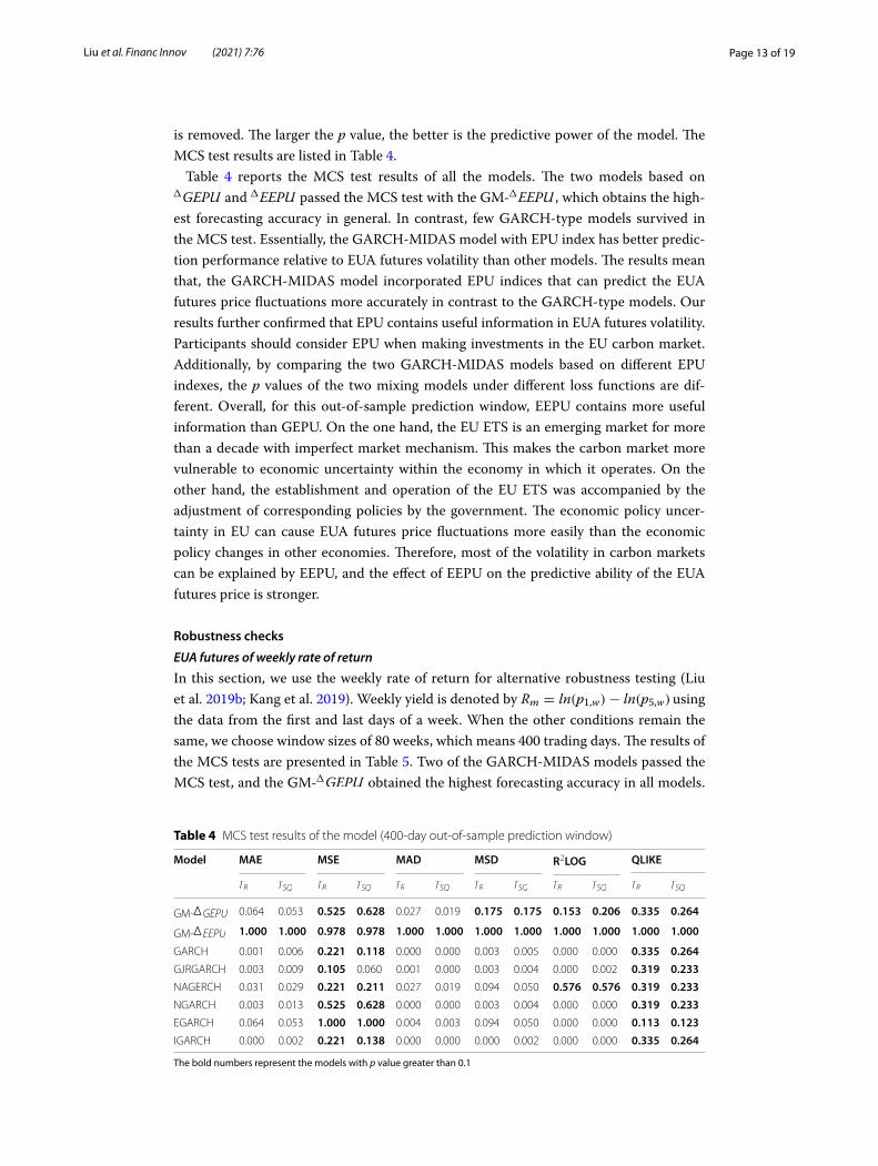
is removed. The larger the p value, the better is the predictive power of the model. The MCS test results are listed in Table 4.

Table  4 reports the MCS test results of all the models. The two models based on �GEPU and �EEPU passed the MCS test with the GM-�EEPU , which obtains the high-est forecasting accuracy in general. In contrast, few GARCH-type models survived in the MCS test. Essentially, the GARCH-MIDAS model with EPU index has better predic-tion performance relative to EUA futures volatility than other models. The results mean that, the GARCH-MIDAS model incorporated EPU indices that can predict the EUA futures price fluctuations more accurately in contrast to the GARCH-type models. Our results further confirmed that EPU contains useful information in EUA futures volatility. Participants should consider EPU when making investments in the EU carbon market. Additionally, by comparing the two GARCH-MIDAS models based on different EPU indexes, the p values of the two mixing models under different loss functions are dif-ferent. Overall, for this out-of-sample prediction window, EEPU contains more useful information than GEPU. On the one hand, the EU ETS is an emerging market for more than a decade with imperfect market mechanism. This makes the carbon market more vulnerable to economic uncertainty within the economy in which it operates. On the other hand, the establishment and operation of the EU ETS was accompanied by the adjustment of corresponding policies by the government. The economic policy uncer-tainty in EU can cause EUA futures price fluctuations more easily than the economic policy changes in other economies. Therefore, most of the volatility in carbon markets can be explained by EEPU, and the effect of EEPU on the predictive ability of the EUA futures price is stronger.

Robustness checks

EUA futures of weekly rate of return

In this section, we use the weekly rate of return for alternative robustness testing (Liu et al. 2019b; Kang et al. 2019). Weekly yield is denoted by Rm = ln(p1,w)− ln(p5,w) using the data from the first and last days of a week. When the other conditions remain the same, we choose window sizes of 80 weeks, which means 400 trading days. The results of the MCS tests are presented in Table 5. Two of the GARCH-MIDAS models passed the MCS test, and the GM-�GEPU obtained the highest forecasting accuracy in all models.

Table 4 MCS test results of the model (400-day out-of-sample prediction window)

The bold numbers represent the models with p value greater than 0.1

Model MAE MSE MAD MSD R2LOG QLIKE

TR TSQ TR TSQ TR TSQ TR TSQ TR TSQ TR TSQ

GM-�GEPU 0.064 0.053 0.525 0.628 0.027 0.019 0.175 0.175 0.153 0.206 0.335 0.264

GM-�EEPU 1.000 1.000 0.978 0.978 1.000 1.000 1.000 1.000 1.000 1.000 1.000 1.000

GARCH 0.001 0.006 0.221 0.118 0.000 0.000 0.003 0.005 0.000 0.000 0.335 0.264GJRGARCH 0.003 0.009 0.105 0.060 0.001 0.000 0.003 0.004 0.000 0.002 0.319 0.233NAGERCH 0.031 0.029 0.221 0.211 0.027 0.019 0.094 0.050 0.576 0.576 0.319 0.233NGARCH 0.003 0.013 0.525 0.628 0.000 0.000 0.003 0.004 0.000 0.000 0.319 0.233EGARCH 0.064 0.053 1.000 1.000 0.004 0.003 0.094 0.050 0.000 0.000 0.113 0.123IGARCH 0.000 0.002 0.221 0.138 0.000 0.000 0.000 0.002 0.000 0.000 0.335 0.264

Page 14 of 19Liu et al. Financ Innov (2021) 7:76

Additionally, few GARCH-type models survived the MCS test. The empirical results confirmed that the predictive power of GARCH-MIDAS with the EPU index is signifi-cantly better than that of the six GARCH-type models. This further suggests that, com-pared with the GARCH-type models, the GARCH-MIDAS model with the EPU index helps enhance the predictive power of EUA futures prices. Basically, the EPU index con-tains more useful information regarding the EU carbon futures price volatility than the GEPU index, which demonstrates the robustness of the above conclusion.

EPU of logarithmic growth rate

According to Fang et  al. (2019), the EPU data are transformed to logarithm growth rates to measure the out-of-sample predictive ability. The new variables are expressed as ∗GEPU and ∗EEPU , where ∗GEPU = ln(GEPUt)− ln(GEPUt−1) , ∗EEPU = ln(EEPUt)− ln(EEPUt−1) . Table  6 reports the MCS results, and we find that only the GM-∗EEPU model survived the MCS test under all loss functions. The GM-∗GEPU model was removed with respect to the MAD and MAE loss functions. However, they outperformed GARCH-type models in most cases. Additionally, all the GARCH-type models survive only under the QLIKE loss function with the TR and TSQ test statistics, and they are eliminated in most cases. This provides strong evidence that

Table 5 MCS test results of the model (80-week out-of-sample prediction window of weekly yield)

The bold numbers represent the models with p value greater than 0.1

Model MAE MSE MAD MSD R2LOG QLIKE

TR TSQ TR TSQ TR TSQ TR TSQ TR TSQ TR TSQ

GM-�GEPU 1.000 1.000 1.000 1.000 1.000 1.000 1.000 1.000 1.000 1.000 1.000 1.000

GM-�EEPU 0.609 0.682 0.720 0.838 0.351 0.325 0.423 0.409 0.922 0.935 0.794 0.790

GARCH 0.126 0.300 0.128 0.398 0.351 0.325 0.082 0.146 0.019 0.199 0.350 0.495GJRGARCH 0.675 0.682 0.872 0.848 0.582 0.473 0.436 0.460 0.922 0.935 0.794 0.790NAGARCH 0.609 0.682 0.720 0.838 0.351 0.325 0.423 0.409 0.922 0.935 0.350 0.495NGARCH 0.093 0.217 0.079 0.187 0.582 0.458 0.082 0.110 0.019 0.042 0.350 0.410EGARCH 0.700 0.700 0.872 0.848 0.886 0.886 0.464 0.464 0.922 0.935 0.597 0.695IGARCH 0.005 0.029 0.004 0.024 0.351 0.325 0.032 0.036 0.019 0.001 0.350 0.328

Table 6 MCS test results of the model (using the logarithmic growth rate of EPU)

The bold numbers represent the models with p value greater than 0.1

Model MAE MSE MAD MSD R2LOG QLIKE

TR TSQ TR TSQ TR TSQ TR TSQ TR TSQ TR TSQ

GM-∗GEPU 0.059 0.059 0.778 0.778 0.024 0.024 0.198 0.198 0.038 0.038 0.881 0.957GM-∗EEPU 1.000 1.000 1.000 1.000 1.000 1.000 1.000 1.000 1.000 1.000 0.881 0.957GARCH 0.000 0.000 0.110 0.159 0.000 0.000 0.000 0.000 0.000 0.000 1.000 1.000GJRGARCH 0.000 0.000 0.368 0.295 0.000 0.000 0.000 0.002 0.000 0.000 0.881 0.957NAGERCH 0.008 0.007 0.566 0.585 0.003 0.003 0.020 0.028 0.001 0.001 0.881 0.957NGARCH 0.000 0.000 0.157 0.188 0.000 0.000 0.000 0.000 0.000 0.000 0.881 0.957EGARCH 0.000 0.000 0.094 0.087 0.000 0.000 0.000 0.000 0.000 0.000 0.881 0.900IGARCH 0.000 0.000 0.094 0.097 0.000 0.000 0.000 0.000 0.000 0.000 0.881 0.957

Page 15 of 19Liu et al. Financ Innov (2021) 7:76

the GARCH-MIDAS models can outperform GARCH-type models, showing the vital role of EPU in enhancing the predictive performance for EUA futures. Additionally, the EEPU can provide more useful information than GEPU, showing its superior ability to predict EUA futures price fluctuations.

Portfolio returns

As EPU indices can be helpful in forecasting the volatility of EUA futures, using the pre-diction results to effectively allocate assets is still significant for investors. In this section, we further explore the economic significance of these models. We consider a mean-var-iance utility investor who allocates his or her assets based on the forecasting volatility between the EUA futures and risk-free assets. Here, we adopt the forecast values of the 400-day out-of-sample window, and the risk-free asset is presented by EONIA rates, a bank overnight rate of the Eurozone [https:// sdw. ecb. europa. eu/]. The portfolio returns of a given time t can be represented as follows:

where ωt is the weight of the portfolio of EUA futures. reua and rf are the yields of the EUA futures and EONIA rates, respectively. r∗eua,t is the excess return, which equals reua,t minus rf . Following Campbell and Thompson (2008) and Zhang et al. (2018), a mean-variance utility investor, the utility function of an investment strategy is equal to:

where γ denotes the risk-aversion coefficient. When the value of γ increases, the risk asset of EUA futures is assigned a lower optimal weight in the portfolio. According to Wang et al. (2016), we set values 3, 6, and 9 for γ for a robustness check. By maximizing the utility function, the optimal portfolio weight can be obtained. It can be expressed as follows:

where r̂∗eua,t+1 is the rolling window forecast of the EUA futures excess return on day

t + 1 and is the corresponding estimate of the excess return volatility on day t + 1. To preclude short sales and prevent more than 50% leverage, we restrict ωt to lie between 0 and 1.5 (Wang et al. 2016). We use the certainty equivalent return (CER) to evaluate portfolio performance.

where µ̂p and σ̂ 2p are the mean and variance of the portfolio during the out-of-sample

period, respectively.Table 7 reports the daily mean excess returns and CER for the eight models over the

400-day out-of-sample period. The GARCH-MIDAS models can generate substantially higher economic returns for the mean-variance investor in contrast to the GARCH-type models. Among all models, the GM-�EEPU model obtains the highest excess returns,

(20)Rp,t = ωt reua,t + (1− ωt)rf ,t = ωt r∗eua,t + rf ,t

(21)U(Rp,t) = Et(Rp,t)− 0.5γVar(Rp,t)

(22)ω∗t =

1

γ

r̂∗eua,t+1

σ̂ ∗eua,t+1

(23)CER = µ̂p −γ

2σ̂ 2p

Page 16 of 19Liu et al. Financ Innov (2021) 7:76

confirming the prediction results above. For larger values of γ , the mean excess return from GM-�EEPU becomes lower but still statistically significant. The results imply that the GARCH-MIDAS model with EPU can not only obtain higher forecasts but also have better performance in portfolio.

ConclusionsIn this study, the GARCH-MIDAS model is adopted to investigate the forecasting per-formance of EPU on EUA futures price volatility. Some noteworthy conclusions were drawn. First, both GEPU and EEPU indexes have remarkable and positive effects on the long-term components of the EU carbon futures market volatility. The results indicate that when EPU increases, the EU carbon market will become more volatile. Policymak-ers, market participants, and especially institutional investors in EU carbon market should be vigilant during the period of high economics policy uncertainty. Second, the GARCH-MIDAS models with variable EPU are superior to the GARCH-type models, and the former can more accurately predict EUA futures price fluctuations. By adding the EPU indices, the forecast performance of EUA futures increases. Additionally, the prediction performance of the GM-

�

EEPU for EUA futures prices is markedly stronger than that of the GM-

�

GEPU . The EU ETS is a burgeoning market for more than a dec-ade with imperfect market mechanisms. This makes the carbon market more vulnerable to economic uncertainty within the economy wherein it operates. Therefore, in the cur-rent phase, emphasizing the EU of EPU when considering the volatility of EUA futures is necessary. The robustness checks further confirm that the EPU index (especially the EPU index of the EU) has strong predictive power for EUA futures prices, and by con-structing a portfolio of EUA futures and risk-free EU rates, the forecast method using EPU indices can produce economic gains for investors in practical applications.

The EU ETS has a high degree of marketization, and the market mechanism tends to become increasingly perfect. However, the higher the degree of marketization, the more sensitive the financial market to economic policy uncertainty (Wang et al. 2014). Hence, we adopt the EPU index to predict EU carbon market fluctuations and confirm its accurate predictive ability. On the one hand, our work is of great value in application. The EPU index offers an effective method for market participants to

Table 7 Portfolio performance over the 400-day out-of-sample period

R is the mean excess returns and CER denotes the certainty equivalent returns. ∗∗ ,∗ indicate significance at the 5% and 10% levels, respectively, under the t‑statistics test. All values were based on days multiplied by 100. Bold numbers represent the largest values for each column

Model γ = 3 γ = 6 γ = 9

R CER R CER R CER

GM-�GEPU 0.132* 0.095 0.065 0.045 0.043 0.029

GM-�EEPU 0.147* 0.111 0.082 ** 0.062 0.057** 0.043

GARCH 0.098 0.076 0.048 0.037 0.032 0.025

GJRGARCH 0.064 0.050 0.031 0.024 0.021 0.016

NAGARCH 0.046 0.036 0.023 0.018 0.015 0.011

NGARCH 0.105* 0.081 0.052 0.040 0.034 0.026

EGARCH 0.093 0.071 0.046 0.035 0.030 0.023

IGARCH 0.098 0.076 0.049 0.037 0.032 0.024

Page 17 of 19Liu et al. Financ Innov (2021) 7:76

manage the risk of price fluctuations. Through the EPU index, investors can con-struct corresponding asset portfolios or design hedge strategies. When the EPU index fluctuates sharply, the EU carbon futures market will also experience large fluctua-tions. By determining whether the uncertainty of economic policies brings positive or negative news, investors can choose to short or long futures markets. Thus, they are more likely to reduce volatility because of the unstable carbon market. Addition-ally, enhancing the ability of the government to correct the implementation of car-bon management strategies. During periods of heightened uncertainty, policymakers can formulate corresponding environmentally oriented policies and regulations to intervene in the carbon futures market. They are apt to avoid excessive fluctuations in price fluctuations caused by increased economic uncertainty by reducing the sup-ply of carbon. Additionally, policymakers must strive to maintain the continuity and stability of policies in the EU carbon market and reduce the uncertainty of economic policies to achieve the long-term goal of promoting the healthy and orderly develop-ment of the EU carbon market. On the other hand, this study has great theoretical significance, as it is an effective complement to existing research on carbon market volatility. Our analysis of the relationship between the EU carbon futures market and EPU is original and may provide a relatively new perspective to measure the volatility of the EU carbon market. Meanwhile, this study could be used as a reference in other carbon market volatility studies.

AbbreviationsEU: European Union; EU ETS: EU emission trading scheme; EPU: economic policy uncertainty; GEPU: Global EPU; EEPU: EU EPU; GARCH-MIDAS: Generalized AutoRegressive conditional heteroskedasticity mixed data sampling; EUA: European Union Allowance; MCS: Model confidence set; ARCH: Autoregressive conditional heteroskedasticity; GJRGARCH: Glosten–Jagannathan–Runkle GARCH; NAGARCH: Nonlinear asymmetric GARCH; IGARCH: Integrated GARCH; NGARCH: nonlinear GARCH; EGARCH: Exponential GARCH; MAE: Mean absolute error; MAD: Mean absolute deviation; MSE: Mean square error; MSD: Mean square deviation; QLIKE: Quasi-maximum likelihood loss function error; R2LOG: Logarithmic likelihood loss function; CER: Certainty equivalent return; QMLE: Quasi-maximum likelihood estimation.

AcknowledgementsThe authors thank the reviewers of this manuscript.

Authors’ contributionsJL conducted the project, checked the initial, first and second revised versions of the paper and approved the final ver-sion. ZZ wrote the paper and revised it. LY checked the third revised versions of the paper and approved the final version. FW conducted the related calculations. All authors read and approved the final manuscript.

FundingThis research was supported by the National Natural Science Foundation of China (Nos. 71871030, 72131011) and the Open Fund Project of Key Research Institute of Philosophies and Social Sciences in Hunan University of China (No. 20FEFMZ1).

Availability of data and materialsThe EUA data that supports the findings of this study are available from the WIND database, but restrictions apply to the availability of these data, because it is not publicly available. The EPU index data are available from http://www.policyuncertainty.com. The data on EONIA rates are available at https://sdw.ecb.europa.eu/.

Declarations

Competing interestsThe authors declare that they have no competing interests.

Author details1 School of Economics and Management, Changsha University of Science and Technology, Changsha, Hunan, People’s Republic of China. 2 School of Business, Hunan Normal University, Changsha, Hunan, People’s Republic of China. 3 Business School, Central South Univerdity, Changsha, Hunan, People’s Republic of China.

Page 18 of 19Liu et al. Financ Innov (2021) 7:76

Received: 19 March 2020 Accepted: 2 September 2021

ReferencesAloui R, Gupta R, Miller SM (2016) Uncertainty and crude oil returns. Energy Econ 55:92–100. https:// doi. org/ 10. 1016/j.

eneco. 2016. 01. 012Alshubiri FN, Tawfik OI, Jamil SA (2020) Impact of petroleum and non-petroleum indices on financial development in

Oman. Financ Innov 6(1):1–22Bahmani-Oskooee M, Saha S (2019) On the effects of policy uncertainty on stock prices: an asymmetric analysis. Quant

Financ Econ 3:412–424. https:// doi. org/ 10. 3934/ QFE. 2019.2. 412Baker SR, Bloom N, Davis SJ (2016) Measuring economic policy uncertainty. Q J Econ 131(4):1593–1636. https:// doi. org/

10. 1093/ qje/ qjw024Balcilar M, Gupta R, Kim WJ, Kyei C (2019) The role of economic policy uncertainties in predicting stock returns and their

volatility for Hong Kong, Malaysia and South Korea. Int Rev Econ Finance 59:150–163. https:// doi. org/ 10. 1016/j. iref. 2018. 08. 016

Bel G, Joseph S (2015) Emission abatement: untangling the impacts of the eu ets and the economic crisis. Energy Econ 49:531–539. https:// doi. org/ 10. 1016/j. eneco. 2015. 03. 014

Bj T, Shen C, Gao C (2013) The efficiency analysis of the European co2 futures market. Appl Energy 112:1544–1547. https:// doi. org/ 10. 1016/j. apene rgy. 2013. 02. 017

Byun SJ, Cho H (2013) Forecasting carbon futures volatility using Garch models with energy volatilities. Energy Econ 40:207–221. https:// doi. org/ 10. 1016/j. eneco. 2013. 06. 017

Campbell JY, Thompson SB (2008) Predicting excess stock returns out of sample: Can anything beat the historical aver-age? Rev Financ Stud 21(4):1509–1531

Challa ML, Malepati V, Kolusu SNR (2018) Forecasting risk using auto regressive integrated moving average approach: an evidence from s&p bse sensex. Financ Innov 4(1):24. https:// doi. org/ 10. 1186/ s40854- 018- 0107-z

Chen X, Li Y, Xiao J, Wen F (2020) Oil shocks, competition, and corporate investment: evidence from china. Energy Econ 104819

Chevallier J (2009) Carbon futures and macroeconomic risk factors: a view from the eu ets. Energy Econ 31(4):614–625. https:// doi. org/ 10. 1016/j. eneco. 2009. 02. 008

Chevallier J (2011) A model of carbon price interactions with macroeconomic and energy dynamics. Energy Econ 33(6):1295–1312. https:// doi. org/ 10. 1016/j. eneco. 2011. 07. 012

Conrad C, Loch K (2015) Anticipating long-term stock market volatility. J Appl Econom 30(7):1090–1114. https:// doi. org/ 10. 1002/ jae. 2404

Conrad C, Schienle M (2020) Testing for an omitted multiplicative long-term component in Garch models. J Bus Econ Stat 38(2):229–242

Conrad C, Loch K, Rittler D (2014) On the macroeconomic determinants of long-term volatilities and correlations in us stock and crude oil markets. J Empir Financ 29:26–40

Davis SJ (2016) An index of global economic policy uncertainty. Technical report, National Bureau of Economic ResearchDhamija AK, Yadav SS, Jain P (2017) Forecasting volatility of carbon under eu ets: a multi-phase study. Environ Econ Policy

Stud 19(2):299–335. https:// doi. org/ 10. 1007/ s10018- 016- 0155-4Dutta A (2019) Impact of carbon emission trading on the European union biodiesel feedstock market. Biomass Bioenerg

128:105328. https:// doi. org/ 10. 1016/j. biomb ioe. 2019. 105328Emenogu NG, Adenomon MO, Nweze NO (2020) On the volatility of daily stock returns of total Nigeria plc: evidence from

Garch models, value-at-risk and backtesting. Financ Innov 6(1):1–25. https:// doi. org/ 10. 1186/ s40854- 020- 00178-1Engle RF, Ghysels E, Sohn B (2013) Stock market volatility and macroeconomic fundamentals. Rev Econ Stat 95(3):776–

797. https:// doi. org/ 10. 1162/ REST_a_ 00300Fan Y, Jia JJ, Wang X, Xu JH (2017) What policy adjustments in the eu ets truly affected the carbon prices? Energy Policy

103:145–164. https:// doi. org/ 10. 1016/j. enpol. 2017. 01. 008Fang L, Yu H, Li L (2017) The effect of economic policy uncertainty on the long-term correlation between us stock and

bond markets. Econ Model 66:139–145. https:// doi. org/ 10. 1016/j. econm od. 2017. 06. 007Fang L, Chen B, Yu H, Qian Y (2018) The importance of global economic policy uncertainty in predicting gold futures

market volatility: a Garch-Midas approach. J Futur Mark 38(3):413–422. https:// doi. org/ 10. 1002/ fut. 21897Fang L, Bouri E, Gupta R, Roubaud D (2019) Does global economic uncertainty matter for the volatility and hedging

effectiveness of bitcoin? Int Rev Financ Anal 61:29–36. https:// doi. org/ 10. 1016/j. irfa. 2018. 12. 010Hansen PR, Lunde A, Nason JM (2011) The model confidence set. Econometrica 79(2):453–497. https:// doi. org/ 10. 3982/

ECTA5 771Hoque ME, Zaidi MAS (2019) The impacts of global economic policy uncertainty on stock market returns in regime

switching environment: evidence from sectoral perspectives. Int J Finance Econ 24(2):991–1016. https:// doi. org/ 10. 1002/ ijfe. 1702

Huang J, Luo Y, Peng Y (2019) Corporate financial asset holdings under economic policy uncertainty: precautionary sav-ing or speculating? Int Rev Econ Finance. https:// doi. org/ 10. 1016/j. iref. 2019. 11. 018

Kanamura T (2019) Supply-side perspective for carbon pricing. Quant Finance Econ 3(1):109. https:// doi. org/ 10. 3934/ QFE. 2019.1. 109

Kang B, Nikitopoulos CS, Prokopczuk M (2019) Economic determinants of oil futures volatility: a term structure perspec-tive. Research paper series

Kautto N, Arasto A, Sijm J, Peck P (2012) Interaction of the eu ets and national climate policy instruments-impact on biomass use. Biomass Bioenerg 38:117–127. https:// doi. org/ 10. 1016/j. biomb ioe. 2011. 02. 002

Page 19 of 19Liu et al. Financ Innov (2021) 7:76

Khan MK, Khan MI, Rehan M (2020) The relationship between energy consumption, economic growth and carbon diox-ide emissions in Pakistan. Financ Innov 6(1):1–13

Koop G, Tole L (2013) Forecasting the European carbon market. J R Stat Soc A Stat Soc 176(3):723–741. https:// doi. org/ 10. 1111/j. 1467- 985X. 2012. 01060.x

Kou G, Akdeniz ÖO, Dinçer H, Yüksel S (2021) Fintech investments in European banks: a hybrid it2 fuzzy multidimensional decision-making approach. Financ Innov 7(1):1–28

Lei L, Yu J, Wei Y, Lai X (2018) Forecasting volatility of Chinese stock market with economic policy uncertainty. J Manag Sci China 1(6):7. https:// doi. org/ 10. 1016/j. physa. 2018. 03. 083

Li X (2019) Economic policy uncertainty and corporate cash policy: international evidence. J Account Public Policy 38(6):106694. https:// doi. org/ 10. 1080/ 00036 846. 2019. 16135 07

Li Y, Ma F, Zhang Y, Xiao Z (2019) Economic policy uncertainty and the Chinese stock market volatility: new evidence. Appl Econ 51(49):5398–5410. https:// doi. org/ 10. 1080/ 00036 846. 2019. 16135 07

Liu HH, Chen YC (2013) A study on the volatility spillovers, long memory effects and interactions between carbon and energy markets: the impacts of extreme weather. Econ Model 35:840–855. https:// doi. org/ 10. 1016/j. econm od. 2013. 08. 007

Liu J, Cheng C, Yang X, Yan L, Lai Y (2019a) Analysis of the efficiency of Hong Kong Reits market based on Hurst exponent. Physica A 534:122035

Liu J, Huang Y, Chang CP (2019b) Leverage analysis of carbon market price fluctuation in china. J Clean Prod 245:118557Mansanet-Bataller M, Pardo A (2009) Impacts of regulatory announcements on co2 prices. J Energy Mark 2(2):1–33.

https:// doi. org/ 10. 21314/ JEM. 2009. 019Mansanet-Bataller M, Pardo A, Valor E (2007) Co2 prices, energy and weather. Energy J. https:// doi. org/ 10. 5547/ ISSN0

195- 6574- EJ- Vol28- No3-5Milunovich G, Joyeux R (2010) Market efficiency and price discovery in the eu carbon futures market. Appl Financ Econ.

https:// ssrn. com/ abstr act= 989272Patton AJ (2011) Volatility forecast comparison using imperfect volatility proxies. J Econom 160(1):246–256Venmans F (2015) Capital market response to emission allowance prices: a multivariate Garch approach. Environ Econ

Policy Stud 17(4):577–620. https:// doi. org/ 10. 1007/ s10018- 015- 0105-6Wang Y, Chen CR, Huang YS (2014) Economic policy uncertainty and corporate investment: evidence from china. Pac

Basin Financ J 26:227–243. https:// doi. org/ 10. 1016/j. pacfin. 2013. 12. 008Wang Y, Ma F, Wei Y, Wu C (2016) Forecasting realized volatility in a changing world: a dynamic model averaging

approach. J Banking Finance 64:136–149. https:// doi. org/ 10. 1016/j. jbank fin. 2015. 12. 010Wei Y, Liu J, Lai X, Hu Y (2017) Which determinant is the most informative in forecasting crude oil market volatility: funda-

mental, speculation, or uncertainty? Energy Econ 68:141–150. https:// doi. org/ 10. 1016/j. eneco. 2017. 09. 016Wen F, Yuan Y, Zhou WX (2019) Cross-shareholding networks and stock price synchronicity: evidence from china. arXiv

preprint arXiv: 19030 1655Yan L, Xu F, Liu J, Teo KL, Lai M (2019) Stability strategies of demand-driven supply networks with transportation delay.

Appl Math Model 76:109–121Yin L (2016) Does oil price respond to macroeconomic uncertainty? New evidence. Empir Econ 51(3):921–938Yu M, Song J (2018) Volatility forecasting: global economic policy uncertainty and regime switching. Physica A 511:316–

323. https:// doi. org/ 10. 1016/j. physa. 2018. 07. 056Yu H, Fang L, Sun W (2018) Forecasting performance of global economic policy uncertainty for volatility of Chinese stock

market. Physica A 505:931–940. https:// doi. org/ 10. 1016/j. physa. 2018. 03. 083Zeitlberger AC, Brauneis A (2016) Modeling carbon spot and futures price returns with Garch and Markov switching

Garch models. CEJOR 24(1):149–176. https:// doi. org/ 10. 1007/ s10100- 014- 0340-0Zha Q, Kou G, Zhang H, Liang H, Chen X, Li CC, Dong Y (2020) Opinion dynamics in finance and business: a literature

review and research opportunities. Financ Innov 6(1):1–22Zhang Y, Ma F, Shi B, Huang D (2018) Forecasting the prices of crude oil: an iterated combination approach. Energy Econ

70:472–483. https:// doi. org/ 10. 1016/j. eneco. 2018. 01. 027Zhang Y, Wei Y, Zhang Y, Jin D (2019) Forecasting oil price volatility: forecast combination versus shrinkage method.

Energy Econ 80(MAY):423–433Zhou K, Li Y (2019) Carbon finance and carbon market in china: progress and challenges. J Clean Prod 214:536–549Zhu B, Chevallier J (2017) European carbon futures prices drivers during 2006–2012. In: Pricing and forecasting carbon

markets, Springer, pp 13–31. https:// doi. org/ 10. 1007/ 978-3- 319- 57618-3_2

Publisher’s NoteSpringer Nature remains neutral with regard to jurisdictional claims in published maps and institutional affiliations.