1

Factors in Implied Volatility Skew in Corn Futures Options

Weiyu Guo* University of Nebraska – Omaha

6001 Dodge Street, Omaha, NE 68182 Phone 402-554-2655

Email: wguo@unomaha.edu

and

Tie Su University of Miami

P.O. Box 248094 Coral Gables, FL, 33124-6552

Phone 305-284-1885 Email: tie@miami.edu

October 20, 2004

JEL Code: G10, G12, G13 Keywords: Commodity futures options, implied volatility, volatility skew. ___________________________ We thank the traders at ConAgra Trade Group, Ankush Bhandri, John Harangody, and Edward Prosser for comments and suggestions. Guo thanks Carl Mammel and Bill Lapp for the faculty-in-residence opportunity at ConAgra Foods, and summer research support from the University Committee on Research at the University of Nebraska at Omaha.

2

Factors in Implied Volatility Skew in Corn Futures Options

Abstract

Empirical studies in options have documented option-implied volatilities obtained at different exercise prices can be dramatically different. Finance professionals call the shape of implied volatility across different option exercise prices “volatility skew” or “volatility smile.” This paper examines factors that affect the slope of the implied volatility skew in corn futures options. We report statistically significant negative impact of option moneyness and option time to maturity on volatility skew.

3

I. Introduction

Option- implied volatility is the volatility imbedded in option prices that reflects the

conditional volatility for the remaining life of the option anticipated by market participants.

Option- implied volatility is not directly observable in the financial markets hence it is often

estimated through a numerical procedure. Estimation of implied volatility is model-dependent.

Different option-pricing model assumptions may yield different implied volatility. Nevertheless,

implied volatility typically is the parameter that equates a theoretical option price to an observed

market option price, given all other known variables, such as the underlying asset price, option

exercise price, option time to maturity, risk-free interest rate, and the dividend or dividend yield,

if any.

It is well-documented that for a given underlying asset and time to maturity, options with

various exercise prices produce different implied volatilities. For example, Rubinstein (1985)

documents that in the equity markets, implied volatility across a range of strike prices for an

option series tends to change as strike price changes and these strike price biases are statistically

significant. This strike price bias is commonly referred as “volatility skew” and the skew pattern

vary. When in-the-money (ITM) and out-of-the-money (OTM) options both have higher implied

volatilities than the at-the-money (ATM) option, the skew pattern is called a “volatility smile” by

option professionals. “Volatility sneer” occurs when ITM and OTM options both are traded at a

lower implied volatility than the ATM option. In the commodity options market, empirical

evidence (e.g., O'Brien Associates Inc. 2000a and 2000b), however, suggest that while volatility

in the OTM options are always higher, the ITM options often have lower implied volatility than

the ATM options. It is believed that this pattern is particularly true when the market is at the

4

lower end of the historical price range where the amount of downside risk perceived by the

market is limited.

The volatility skew phenomena are puzzling because theoretically, implied volatility

should be independent of options’ exercise prices. Option- implied volatility, if correctly

measured, should describe the same unique anticipated return volatility of the underlying asset.

Option-pricing models, such as the Black-Scholes model, hence assumes that for options on the

same underlying asset, the implied volatility across all strikes with the same expiration date

should be the same. The non- linear implied volatility skew curve indicates that in practice,

option market participants maybe be using different volatilities to price options with different

exercise prices. Alternatively, volatility skew can be a result of violations of the underlying

assumptions of the option-pricing model such as the Black-Scholes model or the Black model.

While both the Black-Scholes model and the Black model assume that the return on the

underlying asset is log-normally distributed, Rubinstein (1994) demonstrates that implied

probability distributions obtained from the S&P 500 index options has a thicker tail than a

lognormal distribution at the lower end of the price domain. The thick tail at the low end of the

price domain indicates the market's perception that the actual probability of a market correction

is higher than that predicted by a lognormal distribution. On the contrary, in the commodity

markets, it is generally perceived that the thicker tail occurs at the higher end of the price

domain. The difference in the shapes of the probability densities is due to risk being viewed

differently between the commodity and equity markets. In the financial markets, risk is the

downside movements on asset prices where substantial market capitals would be wiped out. In

the commodity markets, risk is the upside movement on commodity prices which would result in

higher input costs.

5

This paper enriches current literature by examining factors that affect option- implied

volatility skew in the commodity futures option markets. While Ferris, Guo, and Su (2003) and

publications in the industry such as R. J. O'Brien & Associate Inc. (2000a and 2000b) present

summaries of volatility in various agricultural markets such as corn and soybean from 1992 to

1999, this paper goes beyond and focuses on factors that affect option- implied volatility skew in

the corn futures options. It examines how option moneyness and option time to maturity affect

the slope of volatility skew. Our findings have trading implications for option hedgers and

speculators because when an option trader adapts trading strategies such as vertical spreads or

ratio spreads, their positions will be affected not only by changes in the underlying asset price

and option- implied volatility, but also by the shape of the volatility skew.

The rest of the paper is organized as follows: Section II introduces methodology; Section

III describes data; and Section IV presents the empirical results. Conclusions are provided in

Section V.

II. Methodology

Due to its simplicity and mathematical elegance, the Black-Scholes (1973) option-pricing

model has attracted attention from both academia and practitioners alike to price European-style

options on individual stocks, stock indices, currencies, and commodities. An extension of the

Black-Scholes model is the Black (1976) model to price futures options.

The Black (1976) model makes use of five variables to price an European-style futures

option. The five variables are the current futures price (F), the exercise price of the option (X),

the risk free rate of interest (r), the time to option’s maturity (t), and the annualize volatility of

the underlying futures price returns (σ). The first four variables, together with the futures option

6

price, are directly observable from the options and futures markets. However, a trader needs to

estimate the futures price return volatility in order to use the Black option pricing model. If the

options market prices futures options according to the Black model, then the market observed

option price Cobs should be equal to the theoretical option price CBlack generated by the Black

model based on the five inputs as follows:

Cobs = CBlack(futures price, strike, interest rate, time to maturity, volatility)

Solving the equation backward from the observed option prices gives the market option- implied

volatility. We compute an option- implied volatility for each closing quotation of each option

exercise price and time to maturity series on each trading day. We also document the moneyness

and time to maturity of each option for further analysis.

While the Black (1976) model is applicable for European-style futures options, the corn

futures options however, are American-style. A proper model to value American-style options

would be a binomial-tree approach. With all other factors held constant, an American-style

option is always worth more than a European-style option because an American option can be

exercised on or before expiration date while a European option can be exercised only on

expiration. Due to the early exercise premium in American-style options, option- implied

volatility recovered from the Black (1976) model is slightly upward biased for call futures

options. However, the magnitude of the bias is small due to small early exercise premium.

Furthermore, option traders are fully aware of the bias and adjust the option- implied volatility

downward accordingly. In this study, we focus only on call futures options to avoid the early-

exercise of American-style put futures options.

III. Data

7

The data of the study are from the Chicago Board of Trade (CBOT) corn futures options.

The underlying security of the futures options is the corn futures contract which is also traded on

the CBOT. In this study we focus on futures options on September maturity futures contracts

because September contracts are the most heavily traded corn futures contracts.

September futures contracts commence trading every year in May and they expire in

September in the following year. The contract size is 5,000 bushels and the tick size is 1/4 cent

per bushel, or $12.5 per contract. The last day of trading is the last business day prior to the 15th

calendar day of the contract month. The last delivery day is the second business day following

the last trading day of the delivery month. Daily price limit is 20 cents per bushel above or below

the previous day's settlement price. Limits are lifted two business days before the spot month

begins.

Options on the September futures are introduced in June and expire in mid-August of the

following year. Option exercise results in an underlying futures position. Ticker size is 1/8 cent

per bushel, or $6.25 per contract. Strike price interval is five cents per bushel for the most current

two months and 10 cents per bushel for all other months. At the commencement of trading, five

strikes above and five strikes below at-the-money are listed. Except on the last trading day, the

options are subjected to daily price limit of 20 cents per bushel above or below the previous day's

settlement premium. Both the futures contracts and futures option contracts are traded

simultaneously in open outcry from 9:30 a.m. to 1:15 p.m. central time, Monday through Friday.

Our data set contains all daily closing futures and futures option prices for the period of

1991-2000, obtained directly from the CBOT. Price observations before January are excluded

due to thin trading volume on the option contracts, and observations after July are also

8

eliminated due to the short remaining time to expiration. Yields on 90-day Treasury bills are

used as proxy for market risk-free interest rates.

IV. Results

A. Sample description

First we present some descriptive statistics of our raw data. Table 1 summarizes our

findings. The 10-year closing data across different exercise prices yield 24,004 observations.

Note that our sample contains only prices from January up to the end of July for September

maturity contracts. The previous year’s price data are deleted for thin trading. Price data in

August and September before the September maturity are deleted because short-term options are

subject to jump risk in the underlying futures contracts, which is not accounted for in the Black

option-pricing model. Because of the sample screening procedure, the maximum time to maturity

in our sample is around 8.5 months (from beginning of January to mid September) and the

minimum time to maturity is 1.5 months (from end of July to mid September).

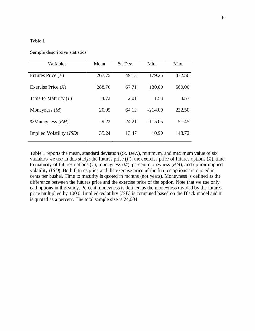
Table 1 presents the mean, standard deviation, minimum, and maximum of six variables

we use in this study: the futures price, the exercise price of futures options, time to maturity of

futures options, moneyness, percent moneyness, and option- implied volatility. Both futures price

and the exercise price of the futures options are quoted in cents per bushel. Time to maturity is

quoted in months (not years). Moneyness is defined as the difference between the futures price

and the exercise price of the option. Note that we use only call options in this study. Percent

moneyness is defined as the moneyness divided by the futures price multiplied by 100. Implied-

volatility (ISD) is computed based on the Black model and it is quoted as a percent.

9

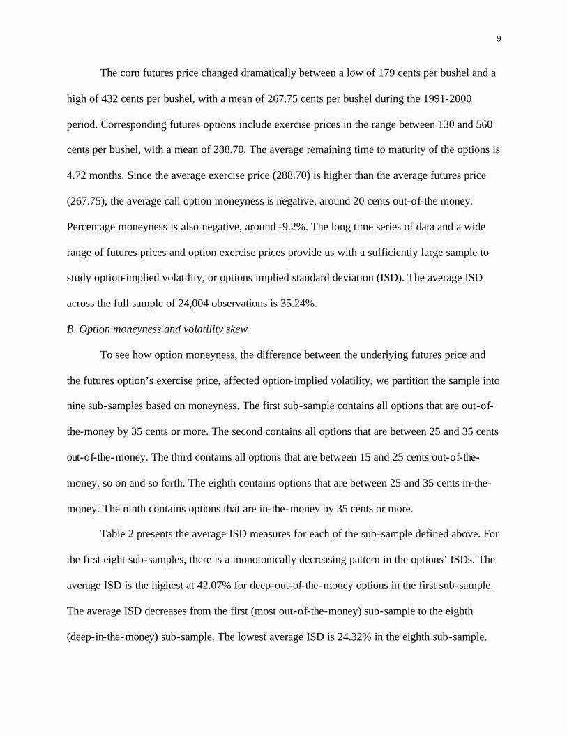
The corn futures price changed dramatically between a low of 179 cents per bushel and a

high of 432 cents per bushel, with a mean of 267.75 cents per bushel during the 1991-2000

period. Corresponding futures options include exercise prices in the range between 130 and 560

cents per bushel, with a mean of 288.70. The average remaining time to maturity of the options is

4.72 months. Since the average exercise price (288.70) is higher than the average futures price

(267.75), the average call option moneyness is negative, around 20 cents out-of-the money.

Percentage moneyness is also negative, around -9.2%. The long time series of data and a wide

range of futures prices and option exercise prices provide us with a sufficiently large sample to

study option-implied volatility, or options implied standard deviation (ISD). The average ISD

across the full sample of 24,004 observations is 35.24%.

B. Option moneyness and volatility skew

To see how option moneyness, the difference between the underlying futures price and

the futures option’s exercise price, affected option- implied volatility, we partition the sample into

nine sub-samples based on moneyness. The first sub-sample contains all options that are out-of-

the-money by 35 cents or more. The second contains all options that are between 25 and 35 cents

out-of-the-money. The third contains all options that are between 15 and 25 cents out-of-the-

money, so on and so forth. The eighth contains options that are between 25 and 35 cents in-the-

money. The ninth contains options that are in- the-money by 35 cents or more.

Table 2 presents the average ISD measures for each of the sub-sample defined above. For

the first eight sub-samples, there is a monotonically decreasing pattern in the options’ ISDs. The

average ISD is the highest at 42.07% for deep-out-of-the-money options in the first sub-sample.

The average ISD decreases from the first (most out-of-the-money) sub-sample to the eighth

(deep-in-the-money) sub-sample. The lowest average ISD is 24.32% in the eighth sub-sample.

10

There is clearly a moneyness effect in volatility skew. However, the decreasing ISD pattern is

not monotonic in moneyness. The ninth sub-sample contains the most in- the-money options. Its

average ISD is 36.47%, which is higher than other in-the-money sub-sample average ISDs.

Figure 1 is a graphic presentation of the results in Table 2, where M in the figure stands

for moneyness of an option. It’s clear that the bar in the far right (the ninth sub-sample) is higher

than all the bars in the middle (sub-samples 2-8).

Figure 2 plots option- implied volatility against option moneyness in the full sample. It is

clear from Figure 2 that option- implied volatility skew displays a “smile” pattern across option

moneyness. The further-away-from-the-money option ISDs are higher than those near-the-

money based on the Black option-pricing model. Note that there are over 24,000 observations

during the period between 1991 and 2000 in our sample. We have also plotted the ISDs on a

year-by-year basis. The pattern persists across each and every calendar year, hence we do not

report the yearly figures. Our results are consistent with previous empirical results on volatility

skew based on stock index options (Rubinstein 1994) and individual stock options, as well as

results from O'Brien Associates Inc. (2000) on agriculture options.

The option- implied volatility “smile” pattern has motivated us to construct a plot of

option- implied volatility against the absolute value of option moneyness. We present the plot in

Figure 3. It shows a clear pattern that as options are further away-from-the-money, option-

implied volatility increases monotonically.

C. Time to maturity and volatility skew

In order to examine how remaining time to maturity affects option- implied volatility, we

partition the sample into eight sub-samples based on time to maturity. The first sub-sample

contains all options that have less than two months to maturity. The second contains all options

11

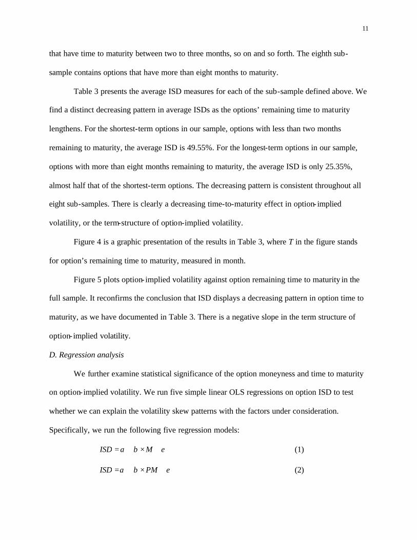
that have time to maturity between two to three months, so on and so forth. The eighth sub-

sample contains options that have more than eight months to maturity.

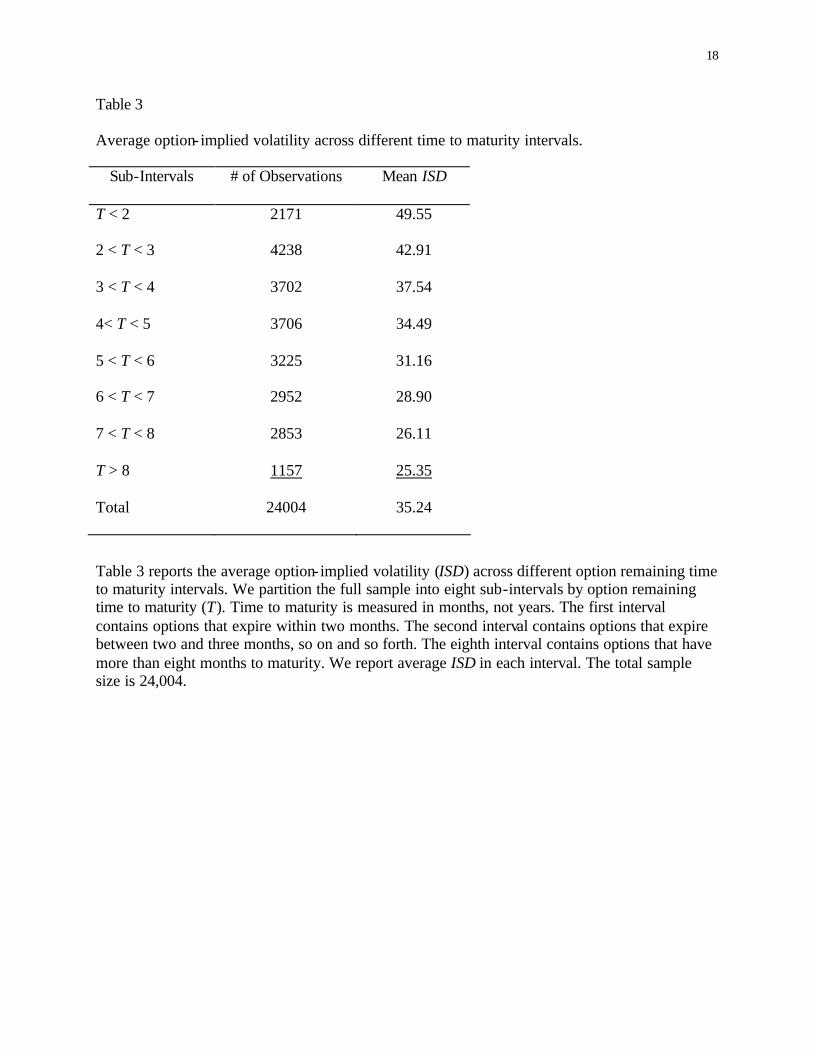
Table 3 presents the average ISD measures for each of the sub-sample defined above. We

find a distinct decreasing pattern in average ISDs as the options’ remaining time to maturity

lengthens. For the shortest-term options in our sample, options with less than two months

remaining to maturity, the average ISD is 49.55%. For the longest-term options in our sample,

options with more than eight months remaining to maturity, the average ISD is only 25.35%,

almost half that of the shortest-term options. The decreasing pattern is consistent throughout all

eight sub-samples. There is clearly a decreasing time-to-maturity effect in option- implied

volatility, or the term-structure of option-implied volatility.

Figure 4 is a graphic presentation of the results in Table 3, where T in the figure stands

for option’s remaining time to maturity, measured in month.

Figure 5 plots option- implied volatility against option remaining time to maturity in the

full sample. It reconfirms the conclusion that ISD displays a decreasing pattern in option time to

maturity, as we have documented in Table 3. There is a negative slope in the term structure of

option- implied volatility.

D. Regression analysis

We further examine statistical significance of the option moneyness and time to maturity

on option- implied volatility. We run five simple linear OLS regressions on option ISD to test

whether we can explain the volatility skew patterns with the factors under consideration.

Specifically, we run the following five regression models:

εβα +×+= MISD (1)

εβα +×+= PMISD (2)

12

εβα +×+= AMISD (3)

εβα +×+= TISD (4)

εγβα +×+×+= TMISD (5)

In the above models, M stands for option moneyness, which is the difference between

underlying futures price and futures option’s exercise price. PM represents percentage

moneyness, computed as 100 times the ratio between option moneyness and underlying futures

price. AM represents the absolute value of the moneyness. T denotes option remaining time to

maturity in months. If option- implied volatility skew is unaffected by these variables, then we

expect all regression slope coefficients to be indistinguishable from zero. However, statistically

significant slope coefficients can lead us to draw conclusions on the impact of these variables on

option- implied volatility skew.

Table 4 documents regression results. In the first model, we find statistical evidence that

option moneyness (M) negatively affect option- implied volatility (ISD). The slope coefficient is

-0.07, which is significant at the 0.0001 level. An increase in option moneyness by one cent

causes decreases in option- implied volatility by 0.07%. Similar results hold for percent

moneyness (PM). Our conclusion does not change for different selections of moneyness

measures.

Motivated by Figure 2 and Figure 3 where further away-from-the-money option- implied

volatilities are higher than near-the-money option- implied volatilities, we regress ISDs on the

absolute value of moneyness (AM). Regression model (3) outlines this procedure. From Table 4,

we find a positively significant slope coefficient on AM, which concludes that option-implied

volatility moves higher as an option moves away from the money. The results are consistent with

intuition gained from Figure 4.

13

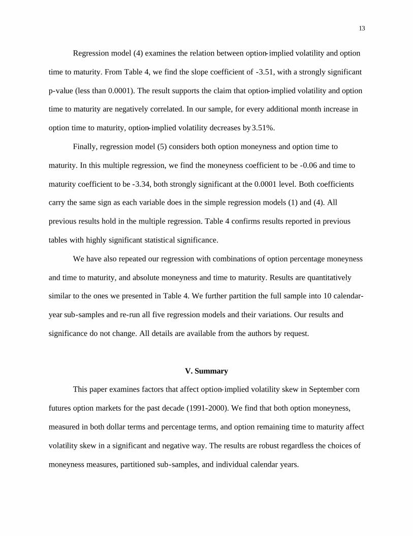
Regression model (4) examines the relation between option- implied volatility and option

time to maturity. From Table 4, we find the slope coefficient of -3.51, with a strongly significant

p-value (less than 0.0001). The result supports the claim that option- implied volatility and option

time to maturity are negatively correlated. In our sample, for every additional month increase in

option time to maturity, option- implied volatility decreases by 3.51%.

Finally, regression model (5) considers both option moneyness and option time to

maturity. In this multiple regression, we find the moneyness coefficient to be -0.06 and time to

maturity coefficient to be -3.34, both strongly significant at the 0.0001 level. Both coefficients

carry the same sign as each variable does in the simple regression models (1) and (4). All

previous results hold in the multiple regression. Table 4 confirms results reported in previous

tables with highly significant statistical significance.

We have also repeated our regression with combinations of option percentage moneyness

and time to maturity, and absolute moneyness and time to maturity. Results are quantitatively

similar to the ones we presented in Table 4. We further partition the full sample into 10 calendar-

year sub-samples and re-run all five regression models and their variations. Our results and

significance do not change. All details are available from the authors by request.

V. Summary

This paper examines factors that affect option- implied volatility skew in September corn

futures option markets for the past decade (1991-2000). We find that both option moneyness,

measured in both dollar terms and percentage terms, and option remaining time to maturity affect

volatility skew in a significant and negative way. The results are robust regardless the choices of

moneyness measures, partitioned sub-samples, and individual calendar years.

14

The results from this paper compare and contrast with other results from empirical

studies in option- implied volatility and volatility skew in stock index options, currency options,

and individual stock options. We provide empirical evidence in corn futures options markets that

are consistent with results from other financial markets in previous research. Non-flat option-

implied volatility skew suggests that the Black model for pricing futures options is mis-specified.

More sophisticated option-pricing models, such as stochastic volatility models, or binomial tree

models should be used in pricing futures options and computing option- implied volatility.

15

References

Black, F. & Scholes, M. (1973). The pricing of options and corporate liabilities. Journal of Political Economy, 81, 3, 637-654. Black, F. (1976). The pricing of commodity contracts. Journal of Financial Economics, 3, 1/2,

167-179. Ferris, S., Guo, W. & Su, T. (2003) Predicting Implied Volatility in the Commodity Futures

Options Markets. International Journal of Finance and Banking, 1, 1, 73-94. R. J. O’Brien & Associate Inc. (2000a). Digging deeper into the volatility aspects of agriculture

options, (1). R. J. O’Brien & Associate Inc. (2000b). Volatility trading in agriculture options, (2). Rubinstein, M. (1994). Implied binomial trees. Journal of Finance, 69, 771-818. Rubinstein, M. (1985). Nonparametric tests of alternative option pricing models using all

reported trades and quotes on the 30 most active CBOE option classes from August 23, 1976 through August 31, 1978. Journal of Finance, 40, 455-480.

16

Table 1

Sample descriptive statistics

Variables Mean St. Dev. Min. Max.

Futures Price (F) 267.75 49.13 179.25 432.50

Exercise Price (X) 288.70 67.71 130.00 560.00

Time to Maturity (T) 4.72 2.01 1.53 8.57

Moneyness (M) 20.95 64.12 -214.00 222.50

%Moneyness (PM) -9.23 24.21 -115.05 51.45

Implied Volatility (ISD) 35.24 13.47 10.90 148.72

Table 1 reports the mean, standard deviation (St. Dev.), minimum, and maximum value of six variables we use in this study: the futures price (F), the exercise price of futures options (X), time to maturity of futures options (T), moneyness (M), percent moneyness (PM), and option- implied volatility (ISD). Both futures price and the exercise price of the futures options are quoted in cents per bushel. Time to maturity is quoted in months (not years). Moneyness is defined as the difference between the futures price and the exercise price of the option. Note that we use only call options in this study. Percent moneyness is defined as the moneyness divided by the futures price multiplied by 100.0. Implied-volatility (ISD) is computed based on the Black model and it is quoted as a percent. The total sample size is 24,004.

17

Table 2

Average option- implied volatility across different moneyness intervals.

Sub-Intervals # of Observations Mean ISD

M < -35 9973 42.07

-35 < M < -250 1463 31.55

-25 < M < -15 1472 30.14

-15 < M < -5 1471 28.71

-5 < M < 5 1473 27.33

5 < M < 15 1447 25.99

15 < M < 25 1329 24.70

25 < M < 35 1097 24.32

M > 35 4279 36.47

Total 24004 35.24

Table 2 reports the average option- implied volatility (ISD) across different moneyness intervals. We partition the full sample into nine sub- intervals by moneyness (M). Moneyness is measured in cents per bushel. The first interval contains options that are out-of-the-money by 35 cents or more. The second interval contains options that are between 25 and 35 cents out-of-the-money, so on and so forth. The eighth interval contains options that are between 25 and 35 cents in-the-money. The last interval contains options that are in-the-money by 35 cents or more. We report average ISD in each interval. The total sample size is 24,004.

18

Table 3

Average option- implied volatility across different time to maturity intervals.

Sub-Intervals # of Observations Mean ISD

T < 2 2171 49.55

2 < T < 3 4238 42.91

3 < T < 4 3702 37.54

4< T < 5 3706 34.49

5 < T < 6 3225 31.16

6 < T < 7 2952 28.90

7 < T < 8 2853 26.11

T > 8 1157 25.35

Total 24004 35.24

Table 3 reports the average option- implied volatility (ISD) across different option remaining time to maturity intervals. We partition the full sample into eight sub-intervals by option remaining time to maturity (T). Time to maturity is measured in months, not years. The first interval contains options that expire within two months. The second interval contains options that expire between two and three months, so on and so forth. The eighth interval contains options that have more than eight months to maturity. We report average ISD in each interval. The total sample size is 24,004.

19

Table 4

Regression results

Parameters Model 1 Model 2 Model 3 Model 4 Model 5

Intercept 33.77 32.99 22.62 51.78 49.70

M -0.07**** -0.06****

PM -0.24****

AM 0.24****

T -3.51**** -3.34****

Adjusted R2 0.11 0.19 0.52 0.27 0.36

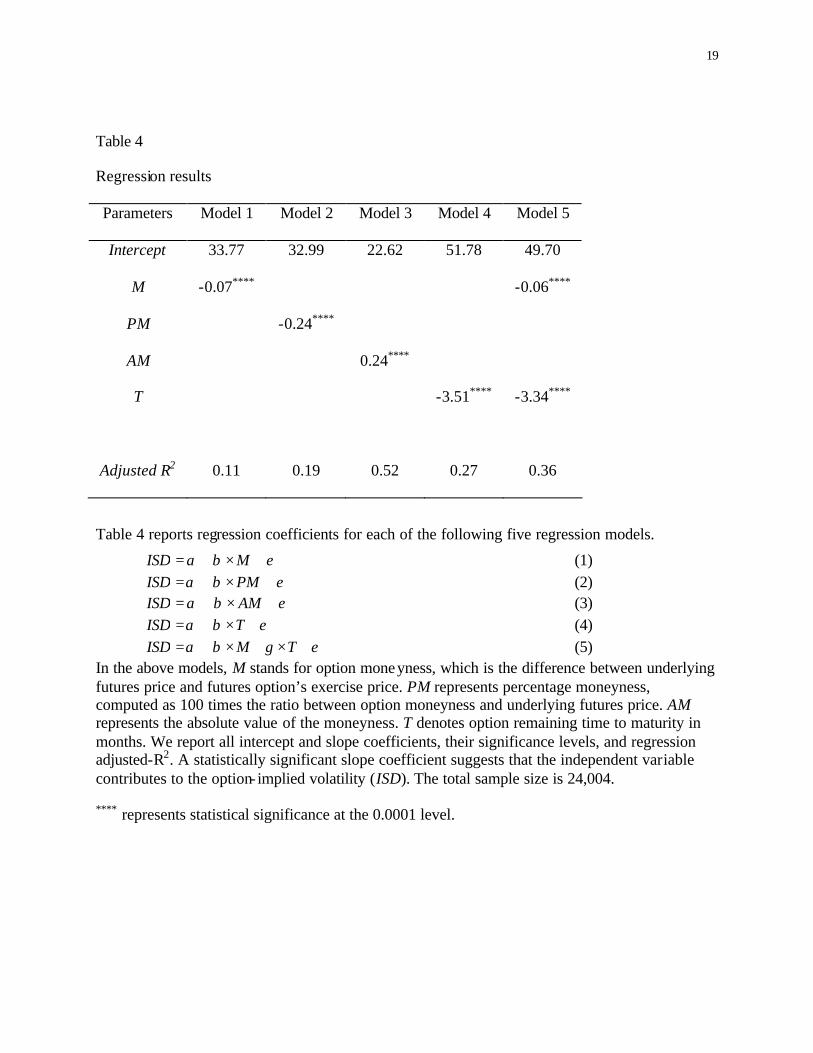
Table 4 reports regression coefficients for each of the following five regression models.

εβα +×+= MISD (1) εβα +×+= PMISD (2) εβα +×+= AMISD (3)

εβα +×+= TISD (4) εγβα +×+×+= TMISD (5)

In the above models, M stands for option moneyness, which is the difference between underlying futures price and futures option’s exercise price. PM represents percentage moneyness, computed as 100 times the ratio between option moneyness and underlying futures price. AM represents the absolute value of the moneyness. T denotes option remaining time to maturity in months. We report all intercept and slope coefficients, their significance levels, and regression adjusted-R2. A statistically significant slope coefficient suggests that the independent variable contributes to the option- implied volatility (ISD). The total sample size is 24,004. **** represents statistical significance at the 0.0001 level.

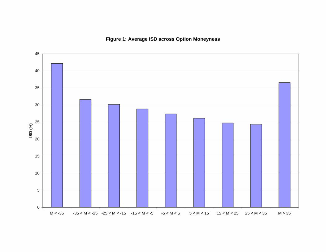
Figure 1: Average ISD across Option Moneyness

0

5

10

15

20

25

30

35

40

45

M < -35 -35 < M < -25 -25 < M < -15 -15 < M < -5 -5 < M < 5 5 < M < 15 15 < M < 25 25 < M < 35 M > 35

ISD

(%

)

Figure 2: ISD vs. Option Moneyness

0

20

40

60

80

100

120

140

160

-250 -200 -150 -100 -50 0 50 100 150 200 250

Option Moneyness (cents)

ISD

(%

)

Figure 3: ISD vs. Absolute Value of Option Percentage Moneyness

0

20

40

60

80

100

120

140

160

0 20 40 60 80 100 120 140

Absolute Value of Option Percentage Moneyness (%)

ISD

(%

)

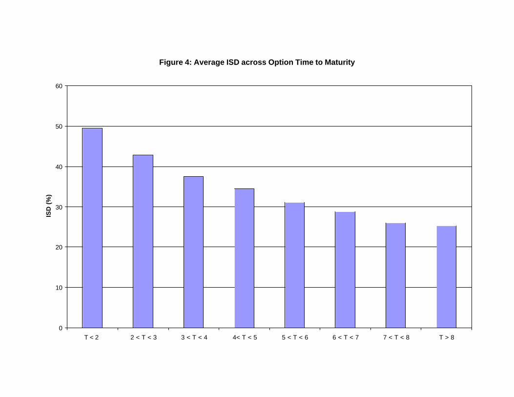
Figure 4: Average ISD across Option Time to Maturity

0

10

20

30

40

50

60

T < 2 2 < T < 3 3 < T < 4 4< T < 5 5 < T < 6 6 < T < 7 7 < T < 8 T > 8

ISD

(%

)

Figure 5: ISD vs. Option Time to Matuirty

0

20

40

60

80

100

120

140

160

0 1 2 3 4 5 6 7 8 9

Time to Maturity (months)

ISD

(%

)