predicting implied volatility in the commodity futures ...moya.bus.miami.edu/~tsu/ijfb2003.pdf · 1...
TRANSCRIPT
Predicting Implied Volatility in the Commodity Futures Options Markets
By
Stephen Ferris* Department of Finance
College of Business University of Missouri - Columbia
Columbia, MO 65211 Phone: 573-882-9905
Email: [email protected]
Weiyu Guo University of Nebraska - Omaha
6001 Dodge Street, Omaha, NE 68182 Phone 402-554-2655 Email: [email protected]
Tie Su University of Miami
P.O. Box 248094 Coral Gables, FL, 33124-6552
Phone 305-284-1885 Email: [email protected]
March 2003 We thank the traders at ConAgra Trade Group, Ankush Bhandri, John Harangody, and Edward Prosser for comments and suggestions. Guo thanks Carl Mammel and Bill Lapp for the faculty-in-residence opportunity at ConAgra Foods, and summer research support from the University Committee on Research at the University of Nebraska at Omaha.

Predicting Implied Volatility in the Commodity Futures Options Markets
Abstract
Academics and practitioners have substantial interest in the implied volatility patterns recovered from commodity futures options. Such knowledge enhances their ability to accurately forecast volatility embedded in these high-risk options. This paper reviews option-implied volatility in the September corn futures option contracts for the period of 1991-2000. It also investigates whether a “weekend effect” exists. We compare forecasting performance of different historical volatility measures. We further report average trading profits of a short straddle strategy, which is motivated by differences between option implied volatility and historical volatility.
JEL Code: G10, G12, G13 Keywords: commodity futures options, implied volatility

1
Predicting Implied Volatility in the Commodity Futures Options Markets
1. Introduction
A call option gives an option holder the right to buy an asset at a price pre-specified in
the option contract on or before the option’s expiration date. The option holder is not obligated to
exercise the option. However, the option holder exercises the option only to increase his own
wealth. Because the option premium reveals the investor's expectation regarding future price
movement by the asset, observed option prices contain information about the market’s expected
price as well as the volatility of the underlying asset. If an option pricing model works well to
price options, then an investor can use the observed option prices to invert the option pricing
model and obtain the market’s estimate of the underlying asset’s volatility. This volatility is
referred to as the option implied volatility.
The importance and usefulness of option implied volatility has been extensively
recognized in the academic literature. Canina and Figlewski (1993) and Fleming (1996, 1998)
examine implied volatilities using S&P 100 stock index options (OEX) while Beckers (1981)
and Lamoureux and Lastrapes (1993) consider options on individual stocks. Day and Lewis
(1993) investigate the nature of implied volatilities on crude oil futures while Jorion (1995)
examines foreign currency futures and Ferri (1996) analyzes foreign currency options. Findings
from Black and Scholes (1973), Merton (1973), Manaster and Rendleman (1982), Day and
Lewis (1992), Ederington and Lee (1996), and Christensen and Prabhala (1998) show that
implied volatilities contain information about the expected variance of stock returns. More recent
work by Mayhew and Stivers (2001) describes the properties of the forecasts contained in option

2
implied volatilities while Ferson, Heuson, and Su (2001) examine the relation between volatility
in stock returns and implied standard deviations.
But the study of implied volatilities has not been limited to equity markets. Wilson and
Fung (1990) examine information content of volatility implied by options on grain futures.
Nelson (1996) studies the relation between option implied volatility and the underlying contract
activity in the live cattle market. Kenyon and Beckman (1997) analyze multiple-year pricing
opportunities for corn and soybeans spot, futures, and futures options markets.
Option implied volatility is of great importance to traders, whether they are hedgers or
speculators. The absolute price level is of secondary importance to traders. It is the change in
price of a futures contract that is important because such changes generate capital gains or losses.
These, in turn, produce trading profits or losses. In addition, fundamental factors such as supply
and demand, traders often look for relations between prices, volumes, open interests, or
volatility. Existing option pricing theories such as Black and Scholes (1973) or Merton (1973)
suggest for instance that there is a positive relation between volatility and option price. When
volatility increases, option prices increase as well and vice versa. Anticipated changes in
volatility generate changes in option prices.
Some commodity traders and academic researchers (Wilson and Fung, 1990; Nelson,
1996) suspect that implied volatility in commodity futures options is seasonal because weather
and other seasonal factors that have the potential to impact crop growth exhibit behaviors that are
predictable in calendar time. If implied volatility is seasonal, then traders can predict volatility
changes based on seasonal patterns. Thus, the first contribution of this study is a test for
seasonality patterns in implied volatilities in corn futures options. We elect to focus on corn
futures contracts since they are the most actively traded agricultural futures contracts on the
3
Chicago Board of Trade (CBOT). Indeed, the average trading volume for this commodity
exceeds 50,000 contracts per day during our sample period, 1991-2000.
Our specific focus is on the September futures option contracts that expire in August.
Volatility in the September futures contracts is the hardest to predict among all such contracts
because of the corn pollination that occurs in July and August. The success of this pollination
period is highly uncertain, thus making the size of the future harvest difficult to assess.
Consequently, September futures contracts are perceived to have a much higher implied
volatility than any other corn futures options. Traders have a substantial interest in the implied
volatility patterns recovered from September futures options because such knowledge enhances
their ability to accurately forecast the volatility embedded in these high-risk options.
Previous studies of the equity market such as French (1980), Lakonishok (1982), Keim,
Stambaugh, and Rogalski (1984) report evidence of a weekly pattern in index returns. This
anomaly is termed the “weekend effect”. Jaffe and Westerfield (1985) and Jaffe, Westerfield,
and Ma (1989) find limited evidence of this effect in international stock markets while Dyl and
Maberly (1986) and Chang, Jain, and Locke (1995) present findings suggesting its presence in
the market for stock index futures.
In this study, we test for a weekend effect in the commodity futures option market by
investigating whether implied volatility is higher on Fridays than Mondays due to added
uncertainty resulting from the market’s weekend closure. Such information will be useful for
traders seeking to find entry or exit points to the market, or to speculate on volatility changes on
a short-term basis.
The final contribution of this study is our analysis of forecasting performance using
alternative measures of historical volatility. We report the forecasting performance of four

4
commonly used historical volatility measures, measured across ten and twenty day moving
windows. In addition, we report the results from executing a short straddle trading strategy using
empirical data. We find positive trading profits when options are within four months to
expiration. We conclude that differences in implied volatilities and historical volatilities lead to
positive trading profits.
We organize the remainder of the paper in the following manner. In section 2 we
introduce our methodology while in section 3 we describe our data and sample construction. We
present our empirical findings in section 4. We discuss the trading implications of our results in
section 5. We conclude with a brief summary in section 6.
2. Methodology
2.1 Implied volatility estimation
Given an option pricing model and an option contract information, the implied volatility
parameter equates the theoretical option price to the observed market option price. The implied
volatility is regarded as the market’s expected volatility of returns for the underlying asset over
the remaining life of the option.
The Black (1976) option pricing model for futures options is a variant of the Black-
Scholes (1973) option pricing model for equity options. Similar to the Black-Scholes model, a
futures price, a strike price, an interest rate, time to maturity, and volatility are used to compute a
futures option price. The first four variables are directly observable from the market. However, a
trader has to estimate the asset return volatility to use any option pricing model. If the market
prices futures options according to the Black model, then the market observed option price, Cobs
should be equal to the theoretical option price, CBlack , generated from the Black model.

5
We use the Black model to recover implied volatilities. The procedure generally requires
a numerical search routine to accomplish this task. Solving the Black model backward from the
observed option prices thus provides an estimate for the option implied volatility.
Because the Black [1976] model is for European style options and the corn futures
options are American style, the binomial pricing model is more appropriate. Other things held
constant, an American style option is always worth more than an otherwise identical European
style option. This is because an American style option can be exercised on or before the
expiration date while a European style option can be exercised only on expiration. Thus for
commodity futures options, the implied volatility recovered from the Black model is upward
biased. This bias however is of minor consequence because most traders are fully aware of it.
Hence, they adjust their estimates accordingly. Furthermore, traders are more concerned with
changes in implied volatility than the absolute level of implied volatility.
2.2 Historical volatility estimations
Historical volatility is estimated by two different procedures: a “standard” procedure and
a “zero-mean” procedure. Figlewski (1997) discusses both procedures in detail. We summarize
these methodologies as follows.
2.2.1 The standard procedure
We begin with a set of historical futures closing prices {S0, S1, ...ST}. We then estimate a
set of log price relatives, i.e., Rt = ln (St/St-1) for t from 1 to T. To obtain historical volatility on a
ten-day moving window basis, the log price relative series is then decomposed into ten-day
internals on a moving window basis. That is, {R1, R2, ...R10}, {R2, R3, ...R11}, and so on. The
historical volatility estimates are the annualized standard deviations of returns for these ten-day
intervals. The numerical expression for the procedure is:

6
( )
0.59 2
2529
t
j tj t
t
R Rσ
+
=
− = ×
∑, t = 1, 2, …, T-9 (1)
where 252 is the number of trading days in a year. tR is the mean return for a 10-day interval,
which is equal to:
91
10
t
t jj t
R R+
=
= ∑ (2)
2.2.2 The zero mean procedure
Figlewski (1997) reports that the mean return of the series is in fact determined only by
the first price observation St-1, the last observation in the price series St+9, and the length of the
interval:
( ) ( )( ) ( ) ( )( )9 9
1 9 1
1 1 1ln ln ln ln
10 10 10
t t
t j j j t tj t j t
R R S S S S+ +
− + −= =
= = − = −∑ ∑ . (3)
Estimating a sample mean based on equation (1) hence can be quite inaccurate. Since the
volatility does not depend heavily on the mean, Figlewski (1997) suggests imposing a sample
mean as zero in the calculation so that historical volatility is estimated by:
0.592
25210
t
jj t
t
Rσ
+
=
= ×
∑, t = 1, 2, …, T-9 (4)
Figlewski (1997) argues that "using elaborate models for mean returns is unlikely to be worth the
effort in terms of any improvement in accuracy". Note that the denominator in equation (4) is ten
instead of nine since the mean is not estimated from the sample, so no observations are lost.

7
Historical volatilities on a 20-day moving window basis are estimated similarly. In the
standard mean procedure,
( )
0.519 2
25219
t
j tj t
t
R Rσ
+
=
− = ×
∑, t = 1, 2, …, T-19 (5)
and in the zero mean procedure:
0.5192
25220
t
jj t
t
Rσ
+
=
= ×
∑, t = 1, 2, …, T-19 (6)
To examine the forecasting performance of the above four historical volatility measures,
we use estimated volatility from a given interval as the volatility forecast for the next interval.
We record the deviations between forecast and realized volatilities. We repeat the above
procedure using 10- and 20-day moving window measures. Root-mean-squared-errors (RMSEs)
summarize all corresponding recorded volatility deviations.
3. Data and Sample Description
3.1 Data description
Both futures and futures option prices in our sample are from the Chicago Board of Trade
(CBOT). They are for Grade No. 2 yellow corn. Pricing data for all expiration months are
available at CBOT. Our sample focuses on all daily closing prices of September futures and
futures option from January to July for the period of 1991-2000. We exclude all option contracts
prior to January because of thin trading volume on the option contracts. We further remove all
observations after July due to the short remaining time to expiration.
8
The underlying asset of a September futures option is September futures contract. For the
futures options, we have data concerning the option premium, strike price, maturity month,
underlying security price, and T-bill rates. We recover the option implied volatility from at-the-
money options. When the futures price does not exactly equal any strike price, we use a near the
money option to approximate an at-the-money option. The Black (1976) model requires a market
interest rate to compute an option price. We first use a six percent constant risk free rate in the
Black model. Some traders often use a constant interest rate because the impact of interest rate
on the recovered implied volatility is believed to be trivial and should not materially impact
trading decisions. We also use yields on 90-day Treasury bills as more elaborate proxies for
market interest rates. Our tables present results from both sets of market interest rate proxies.
3.2 Nature of the contract
The September corn futures contracts are introduced in May each year and expire in
September of the following year. The contract size is 5,000 bushels and the tick size is 1/4 cent
per bushel. The daily price limit is 20 cents per bushel above or below the previous day's
settlement price. Limits are lifted two business days before the spot month begins.
Options on the September futures are introduced in June and expire in mid-August of the
following year. Option exercise results in an underlying futures market position. The tick size is
1/8 cent per bushel. The strike price interval is five cents per bushel for the most current two
months and ten cents per bushel for all other months. At the commencement of trading, five
strikes above and five strikes below at the money are listed. Except on the last trading day,
options are subjected to a daily price limit of 20 cents per bushel above or below the previous
day's settlement premium. Both the futures contracts and futures option contracts are traded

9
simultaneously in open outcry from 9:30 a.m. to 1:15 p.m. This characteristic reduces potential
noise that could result from non-synchronous trading, as occurs in index and index options.
4. Empirical results
4.1 Implied volatility
We use the Black (1976) model to estimate option implied volatility of September corn
futures options. First, for each trading day, our sample provides us with a set of input variables.
They include the September corn futures closing price, option time to maturity, option strike
price, market interest rate, and option premium. Second, we program a numerical search routine
to compute an asset return volatility that equates the Black futures price to the observed market
price. Since the option price is monotonic in volatility, the search routine quickly converges to a
unique solution. We repeat the procedure for each trading day in our sample and document all
daily implied volatilities in our ten-year sample period for further analysis.
4.2 Patterns in annual implied volatilities
Table 1 reports the average implied volatility over each month during our sample period.
Figure 1 is a graphical presentation of those results. Over our ten-year sample period, we observe
a rising trend in volatility from January to July. Implied volatilities are the lowest in January and
increase steadily from January to May. They continue to increase from the planting season in
May and remain high going into the July pollination season. The mean option implied volatility
increases by more than 25% from January (23.00%) to May (29.15%). The results are robust
with respect to the selection of an interest rate proxy.
<Figure 1 about here>

10
<Table 1 about here>
We plot annual implied volatility patterns in Figure 1. In 1991, implied volatility started
at around 20% and gradually rose to over 30% in mid-July during the pollination period. In 1993,
implied volatility remained at the 20% level for the beginning of the year, increased in March,
declined and then temporarily jumped to slightly over 30% going into July and finally fell to
below 30% during pollination. The implied volatility patterns are somewhat similar for 1992 and
1994. In both years, implied volatility dramatically rose in May and remained high until the end
of June before declining to around 20% in July. This suggests that the market expected high
uncertainty in corn yield in May, but the uncertainty was reduced during pollination. In 1995,
volatility started to increase in mid-March and remained high as pollination approached. The
year 1996 experienced a high level of volatility. Volatility rose dramatically in mid-April and
stayed high as pollination approached, but fell slightly during the actual pollination season. In
1997, higher uncertainty occurred during pollination period. In 1998, the market started on the
high end of the volatility range from the beginning and ended lower in late July. In 1999,
volatility consistently increased throughout the first half of the year with high volatility entering
July. The pattern in year 2000 is different from that of the other years. Market implied volatility
started from above 30% at the beginning of the year. It went up to as high as over 40% in May,
and remained above 30% before finally dropping below 30% in late July.
Our findings suggest that it is difficult to find evidence of seasonal patterns that apply to
even a majority of our sample years. Weather, price stagnation, and the pace of planting are all
factors that significantly impact corn yield. While current production plus ending stock from
prior year establish the supply side of the equation, domestic usage and global demand determine
11
demand. The imbalance between supply and demand result in changes in market price as well as
market implied volatility. Kluis (1998) notes that technological changes, the impact of
commodity funds, and international trade combine to make the commodity market more
sensitive and responsive to new, economically relevant information. These changes result in
higher short-term market volatility. These market volatility changes are then captured in the
annual volatility patterns discussed above.
4.2 Weekend effect
Another question that puzzles commodity traders is whether implied volatility is higher
on Fridays than on Mondays due to the uncertainty resulting from a market that has been closed
over the weekend. In short, is there a weekend effect in implied volatilities? Insights on this
question are useful as traders seek to find market entry or exit points or to speculate on short-
term volatility changes.
Table 2 reports the means in weekday volatility. We find that the mean volatility on
Friday (27.49%) is slightly higher than that on Monday (27.21%). This result is consistent with
Chang, Jain, and Locke (1995) who find that Friday's close is the period of highest volatility in
the S&P 500 futures market. However, the differences between the Friday and Monday means
are small and statistically insignificant. Although economically relevant activity might occur
during the weekend, the mean option implied volatility does not appear to be affected. We
conclude that there is not a weekend effect in option implied volatilities.
<Table 2 about here>
4.3 Historical volatility
Historical volatility in general begins at a lower level during the early part of the year,
rises at a faster pace than option implied volatility does during mid-year, but approaches implied
12
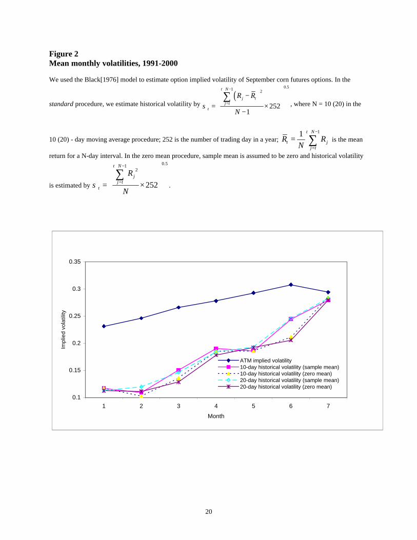
volatility near the option expiration date. Figure 2 illustrates monthly averages of ten and twenty
day moving window historical standard volatility measures and the mean option implied
volatility. Since historical volatility measures are estimated from historical futures prices, a
possible explanation for lower historical volatility in the early part of a year is the “non-trading
effect" (Figlewski, 1997). When the futures markets are relatively less active at the beginning of
the year, the full impact of a large information event tends to spread over two or more days'
recorded closing prices, which would result in positive autocorrelation in returns. The
autocorrelation in return reduces estimated volatility. When the futures markets become more
active, futures prices become more volatile and we observe higher historical volatilities.
<Figure 2 about here>
Table 3 reports the average historical volatilities by month for each year. We also observe
an increasing trend in the realized historical volatilities from January to July. The results are
consistent with those presented in Table 1.
Table 4 reports the forecasting performance of the four different historical volatility
measures. The root-mean-squared-errors (RMSEs) measure the forecasting performance. The
smaller the RMSE, the better the forecast. RMSE indicate that the 20-day zero mean historical
volatility gives best forecasting results among all four historical volatility measures. The 20-day
standard historical volatility performs the second best.
<Table 4 about here>
5. Trading implications
While some corn traders suspect that corn futures option implied volatility might be
seasonal due to the fact that corn growth is affected by many seasonal factors, a close

13
examination of the volatility pattern for the decade of the 1990s reveals that volatility is not as
seasonal as suspected. The volatility is largely affected by the impact of weather on the planting,
pollination, and growth of the corn crop. Although a general rising trend of implied volatility
from January to July is observed, time decay may offset the gains in option prices that result
from higher volatility.
Traders frequently compare implied volatility with historical volatility from the same
period from prior years to predict short-term implied volatility changes. Historical volatility
tends to be lower than implied volatility in the early part of a year. This pattern, however, does
not necessarily imply a trading opportunity. Still, we are curious about the potential for profit
resulting from the difference in implied and realized volatilities. If implied volatility is
consistently larger than realized volatility in futures contracts, then the futures options will tend
to be over-priced.
A short options straddle, which involves a short call option and a short put option on the
same underlying asset, with the same time to maturity and exercise price, should generate a
profit. These short straddles are also called volatility strategies, or volatility plays. Holders of
short straddles gain if the market price at maturity stays within a narrow range around the
straddle’s strike price. This assumes that the positions are held to maturity without delta neutral
hedging1.
We simulate this trading strategy with empirical futures and futures options data. On each
trading day in our sample, we construct a short straddle by using an at-the-money call and a put
option pair. The call and the put share the same at-the-money strike price and the same maturity
1 Traders are likely to create a delta neutral hedge to protect against losses from an adverse movement in futures prices. A delta-neutral hedge involves a long position in a fraction of a unit of the underlying asset and a short call contract. For small changes in the underlying asset, the overall portfolio value is unchanged. Consequently, the portfolio is called a hedged portfolio. Delta refers to the hedge ratio, i.e., the fraction of shares that needs to hedge a short call.
14
month (September). We collect options premiums (C0 + P0) for the call and the put on the set up
day. We hold the short straddle until the options matures and then compute the payoff, which is
|FT – X|. This strategy generates a dollar profit/loss of W and a percent return of R:
W = C0 + P0 - |FT – X| (7)
R = W / (C0 + P0) (8)
We define C0 as the call option premium on the set up day, P0 as the put option premium
on the set up day, FT as the futures price on the expiration day, and X as the strike price of the
call and put.
Table 5 contains the average dollar and percent returns across each of the months during
our sample period. We report the results by month. Average dollar profits are quoted on a cents
per bushel basis while percent return is quoted as a percent of the initial call and put premiums
collected, as defined in equation (8). In the first three months of each year, the average dollar
profits are negative, suggesting that the short straddles lose money on average. The results are
not surprising because of the long holding period. There is a lot of risk in the underlying futures
contract. Holding a short straddle on these contracts involves is risky. Our empirical results show
that there is no benefit, on average, in a short straddle strategy during the months of January,
February, and March. However, average trading profits for the months between April and July
are significantly positive. The highest average trading profit occurs in the month of April. The
mean is 6.87 cents per bushel, which corresponds to a return of 16.32%. These statistics are both
statistically and economically significant. Consider a six-cent per bushel profit. Since the
contract size of corn futures is 5,000 bushels, the profit directly translates to $300 per contract
($0.06×5,000 = $300).
<Table 5 about here>

15
We argue that the positive trading profits are closely related to the fact that option
implied volatilities are visibly larger than realized volatilities as presented in Figure 2. High
implied volatility leads to high option prices, which lead to profits on short options straddles.
Since realized volatilities are lower than implied volatilities, the underlying futures contracts do
not generate the degree of movement anticipated by option traders. Consequently, short straddles
produce positive profits.
However, we must interpret the results with caution. First, in our computation, we
ignored market frictions, including but not limited to, bid/ask spread and transaction costs.
Including such factors will clearly reduce profits and increase losses. Traders face these costs.
Spread and transaction adjusted profits and losses are more meaningful in such a calculation.
Second, options on futures are highly risky securities. Short futures option straddles are highly
risky speculative positions. A close examination of Table 5 reveals the standard deviations of the
trading returns are in the neighborhood of 60%, and the maximum loss can go well beyond
-100% (-233.87% in the month of July). It is true that the average trading profits are positive.
However, it is not clear that the average risk-adjusted returns on the short straddles are still
positive.
6. Conclusion
This paper examines volatility embedded in the September corn futures option markets for
the sample period, 1991-2000. Our analysis focuses on the corn futures contracts since they are
the most actively traded agricultural futures contract on the CBOT. We find an increase trend in
both the implied volatility and historical volatility in September corn futures contract over
January to July period. However, it is difficult to find any other genuine annual seasonal pattern

16
that fits all the years. Weather, price stagnation and the pace of planting all exert an influence on
market price and volatility. Implied volatility on Fridays, in general, is higher than that on
Mondays. However, the differences are small and statistically insignificant. Historical volatility
in general is lower than option implied volatility in the earlier part of the year. However,
historical volatility rises at a faster pace than implied volatility during mid-year and approaches
implied volatility near the option expiration date. Short straddle positions generate positive
profits only when futures options are within four months to expiration. The average returns are
positive with a large variance. The root-mean-squared-errors (RMSEs) indicate that 20-day
moving window zero mean historical volatility measures gives the best forecasting results among
all four candidates we consider in this study.
17
References
Beckers, S., 1981. Standard deviations implied in option prices as predictors of future stock price variability. Journal of Banking and Finance 5, 363-82.
Black, F., 1976. The pricing of commodity contracts. Journal of Financial Economics 3, 167-179.
Black, F., and Scholes, M., 1973. The pricing of options and corporate liabilities. Journal of Political Economy 81, 637-654.
Canina, L., and Figlewski, S., 1993. The informational content of implied volatility. Review of Financial Studies 6, 659-81.
Chang, E., Jain, P., and Locke, P., 1995. Standard & Poor's 500 index futures volatility and price changes around the New York Stock Exchange close. The Journal of Business 68(1), 61-84.
Christensen, B., and Prabhala, N., 1998. The Relation between implied and realized volatility. Journal of Financial Economics 50, 125-150.
Day, T., and Lewis, C., 1992. Stock market volatility and the information content of stock index options. Journal of Econometrics 52, 267-287.
Day, T., and Lewis, C., 1993. Forecasting futures market volatility. Journal of Derivatives 1, 33-50.
Dyl, E., and Maberly, E., 1986. The weekly pattern in stock index futures: A further note. The Journal of Finance 41(5), 1149-1152.
Ederington, L., and Lee, J., 1996. The creation and resolution of market uncertainty: The impact of information releases on implied volatility. Journal of Financial and Quantitative Analysis 31, 513-539.
Ferri, A., 1996. Unpublished Dissertation Research. New York University Stern School of Business.
Ferson, W., Heuson, A., and Su, T., 2001. How much do expected stock returns vary over time? Answers from the options market. Working paper. University of Miami.
Figlewski, S., 1997. Forecasting volatility. In: Financial Markets, Institutions, and Instruments. Boston MA: Blackwell Publishers, Vol.6, No.1.
Fleming, J., 1996. The quality of market volatility forecasts implied by S & P 100 index options prices. Working paper. Jones Graduate School, Rice University.
Fleming, J., 1998. The quality of market volatility forecasts implied by the S&P 100 index options. Journal of Empirical Finance 5, 317-346.
French, K., 1980. Stock returns and the weekend effect. Journal of Financial Economics 8(1), 55-69.
Jaffe, J., Westerfield, R., 1985. The week-end effect in common stock returns: The international evidence. The Journal of Finance 40(2), 433-454.

18
Jaffe, J., Westerfield, R., and Ma, C., 1989. A twist on the Monday effect in stock prices: Evidence from the U.S. and foreign stock markets. Journal of Banking & Finance 13(4,5), 641-650.
Jorion, P., 1995. Predicting volatility in the foreign exchange market. Journal of Finance 50, 507-28.
Keim, D., Stambaugh, R., and Rogalski, R., 1984. A further investigation of the weekend effect in stock returns/discussion. The Journal of Finance 39(3), 819-837.
Kenyon, D., and Beckman, C., 1997. Multiple-year pricing strategies for corn and soybeans. Journal of Futures Markets 17(8) 909-934.
Kluis, A., 1998. Marketing patterns have changed. Soybean Digest August/September .
Lakonishok, J., and Maurice L., 1982. Weekend effects on stock returns: A note. The Journal of Finance 37(3), 883-889.
Lamoureux, C., and Lastrapes, W., 1993. Forecasting stock-return variance: Toward an understanding of stochastic implied volatilities. Review of Financial Studies 6(2), 293-326.
Manaster, S., and Rendleman, Jr., R., 1982. Option prices as predictors of equilibrium stock prices. Journal of Finance 37, 1043-1057.
Mayhew, S., and Stivers, C., 2001. Estimating stock return dynamics using implied volatilities. Working paper. University of Georgia.
Merton, R., 1973. The theory of rational option pricing. Bell Journal of Economics and Management Science 4, 141-183.
Nelson, J., 1996. The “other” live cattle market: Implied volatility. Futures 25(10), 46-48.
Wilson, W., and Fung, H., 1990. Information content of volatilities implied by option premiums in grain futures. Journal of Futures Markets 10(1), 13-27.

19
Figure 1Option implied volatility for September corn futures, 1991-2000We use the Black[1976] model to estimate the option implied volatility. Specifically, we program a numerical search routine to compute an asset return volatility that equates a Black futures price to an observed market price. The procedure is repeated for each trading day in our sample. DailyATM option implied volatility (IV) is reported below with IV on the vertical axis, and year and months on the horizontal axis. Yields on 90-day T-bill are used as market interest rate proxies.
0%10%20%30%40%50%60%
1-Jan
31-Jan
1-Mar
31-Mar
30-Apr
30-May
29-Jun
29-Jul
2000
IV
0%10%20%
30%40%50%60%
1-Jan
31-Jan
2-Mar
1-Apr
1-May
31-May
30-Jun
30-Jul
1991
IV
0%10%20%30%40%50%60%
2-Jan
1-Feb
2-Mar
1-Apr
1-May
31-May
30-Jun
30-Jul
1992
IV
0%10%20%30%40%50%60%
1-Jan
31-Jan
2-Mar
1-Apr
1-May
31-May
30-Jun
30-Jul
1993
IV
0%10%20%30%40%50%60%
1-Jan
31-Jan
2-Mar
1-Apr
1-May
31-May
30-Jun
30-Jul
1994
IV
0%10%20%30%40%50%60%
1-Jan
31-Jan
2-Mar
1-Apr
1-May
31-May
30-Jun
30-Jul
1995
IV
0%10%20%30%40%50%60%
1-Jan
31-Jan
1-Mar
31-Mar
30-Apr
30-May
29-Jun
29-Jul
1996
IV
0%10%20%30%40%50%60%
1-Jan
31-Jan
2-Mar
1-Apr
1-May
31-May
30-Jun
30-Jul
1997
IV
0%10%20%30%40%50%60%
1-Jan
31-Jan
2-Mar
1-Apr
1-May
31-May
30-Jun
30-Jul
1998
IV
0%10%20%30%40%50%60%
1-Jan
31-Jan
2-Mar
1-Apr
1-May
31-May
30-Jun
30-Jul
1999
IV
20
Figure 2 Mean monthly volatilities, 1991-2000 We used the Black[1976] model to estimate option implied volatility of September corn futures options. In the
standard procedure, we estimate historical volatility by ( )
0.51 2
2521
t N
j tj t
t
R R
Nσ
+ −
=
−
= ×−
∑, where N = 10 (20) in the
10 (20) - day moving average procedure; 252 is the number of trading day in a year; 11 t N
t jj t
R RN
+ −
=
= ∑ is the mean
return for a N-day interval. In the zero mean procedure, sample mean is assumed to be zero and historical volatility
is estimated by
0.512
252
t N
jj t
t
R
Nσ
+ −
=
= ×
∑.
0.1
0.15
0.2
0.25
0.3
0.35
1 2 3 4 5 6 7
Month
Impl
ied
vola
tility
ATM implied volatility10-day historical volatility (sample mean)10-day historical volatility (zero mean)20-day historical volatility (sample mean)20-day historical volatility (zero mean)

21
Table 1 Mean implied volatility based on at-the-money calls by month for 1991-2000
The Black (1976) model is used to estimate the option implied volatility of September corn futures options. For each trading day, our sample provides us with a set of input variables including futures closing price, option time to maturity, option strike price, market interest rate, and option premium. We program a numerical search routine to compute an asset return volatility that equates the Black futures price to the observed market price. We repeat the procedure for each trading day in our sample and document all daily implied volatilities in our ten-year sample period.
Panel A: The interest rate is derived from yields on 90-day T-bills Year January February March April May June July 1991 0.2278 0.2293 0.2391 0.2420 0.2261 0.2479 0.3036 1992 0.2289 0.2565 0.2479 0.2343 0.2727 0.3275 0.2260 1993 0.2112 0.2015 0.2351 0.2364 0.2213 0.2272 0.3006 1994 0.2075 0.2201 0.2290 0.2441 0.2856 0.3508 0.2102 1995 0.1943 0.2035 0.2286 0.2547 0.2725 0.2969 0.2943 1996 0.2214 0.2512 0.2668 0.3536 0.3746 0.3699 0.3579 1997 0.2236 0.2449 0.2899 0.2902 0.2670 0.2539 0.2807 1998 0.2578 0.2752 0.2953 0.2737 0.2971 0.3323 0.2655 1999 0.2390 0.2593 0.2921 0.3016 0.3196 0.3310 0.3845 2000 0.2875 0.2963 0.3244 0.3316 0.3723 0.3367 0.3109 1991-2000 average 0.2300 0.2441 0.2647 0.2765 0.2915 0.3076 0.2936 Panel B: The interest rate is set at six percent Year January February March April May June July
1991 0.2280 0.2296 0.2379 0.2425 0.2265 0.2483 0.3037 1992 0.2320 0.2596 0.2501 0.2363 0.2745 0.3290 0.2268 1993 0.2150 0.2054 0.2370 0.2390 0.2233 0.2276 0.3015 1994 0.2115 0.2236 0.2317 0.2461 0.2874 0.3524 0.2103 1995 0.1950 0.2047 0.2288 0.2537 0.2728 0.2973 0.2945 1996 0.2224 0.2526 0.2672 0.3560 0.3756 0.3670 0.3582 1997 0.2249 0.2461 0.2910 0.2903 0.2682 0.2538 0.2810 1998 0.2594 0.2764 0.2964 0.2750 0.2983 0.3330 0.2658 1999 0.2411 0.2614 0.2937 0.3031 0.3210 0.3320 0.3849 2000 0.2885 0.2974 0.3247 0.3325 0.3736 0.3369 0.3107 1991-2000 average 0.2313 0.2460 0.2658 0.2777 0.2927 0.3080 0.2941

22
Table 2 Mean implied volatility based on at-the-money calls by day of week, 1991-2000
The Black (1976) model is used to recover implied volatilities. Solving the Black model backward from the observed option prices provides an estimate for the option implied volatility.
Panel A: The interest rate is derived from yields on 90-day T-bills Monday Tuesday Wednesday Thursday Friday Mean 0.2721 0.2731 0.2728 0.2721 0.2749 Standard Dev. 0.0518 0.0531 0.0529 0.0520 0.0568
Panel B: The interest rate is set at six percent Monday Tuesday Wednesday Thursday Friday Mean 0.2741 0.2744 0.2738 0.2727 0.2753 Standard Dev. 0.0520 0.0525 0.0529 0.0517 0.0565

23
Table 3 Mean historical volatility by month, 1991-2000
In the standard procedure, we estimate historical volatility by ( )
0.51 2
2521
t N
j tj t
t
R R
Nσ
+ −
=
−
= ×−
∑, where
N = 10 (20) in the 10 (20) - day moving average procedure; 252 is the number of trading day in a year; 11 t N
t jj t
R RN
+ −
=
= ∑ is the mean return for a N-day interval. In the zero mean procedure, sample mean is
assumed to be zero and historical volatility is estimated by
0.512
252
t N
jj t
t
R
Nσ
+ −
=
= ×
∑.
Standard procedure Zero mean procedure
10-day historical volatility
10-day historical volatility (zero mean)
Month
Max
Min
Mean
Std.
Max
Min
Mean
Std.
Jan 0.2405 0.0358 0.1171 0.0528 0.2322 0.0350 0.1173 0.0534 Feb 0.3154 0.0280 0.1094 0.0552 0.2039 0.0279 0.1024 0.0389 Mar 0.4142 0.0483 0.1506 0.0781 0.2883 0.0473 0.1361 0.0538
Apr 0.5735 0.0489 0.1905 0.1026 0.5659 0.0471 0.1853 0.1020 May 0.3915 0.0775 0.1860 0.0687 0.3786 0.0761 0.1856 0.0685 Jun 0.8618 0.0639 0.2445 0.1578 0.4592 0.0733 0.2114 0.0798 Jul 0.4926 0.0814 0.2792 0.0969 0.5021 0.1166 0.2847 0.0935
20-day historical volatility
20-day historical volatility (zero mean)
Month
Max
Min
Mean
Std.
Max
Min
Mean
Std.
Jan 0.1918 0.0521 0.1130 0.0376 0.1932 0.0517 0.1127 0.0377 Feb 0.2266 0.0449 0.1198 0.0490 0.1988 0.0441 0.1113 0.0381 Mar 0.3120 0.0577 0.1461 0.0667 0.2497 0.0577 0.1286 0.0456 Apr 0.4353 0.0672 0.1843 0.0803 0.4356 0.0716 0.1781 0.0820 May 0.4227 0.0975 0.1932 0.0743 0.4120 0.0952 0.1918 0.0733 Jun 0.6381 0.0972 0.2454 0.1390 0.3700 0.0947 0.2057 0.0662 Jul 0.4362 0.1435 0.2831 0.0708 0.4280 0.1407 0.2796 0.0680

24
Table 4 Forecasting performance of historical volatility estimates for 1991-2000
We use estimated volatility from a given interval as the volatility forecast for the next interval. We record the deviations between forecast and realized volatilities. We repeat the above procedure using 10- and 20-day moving window measures. Root-mean-squared-errors (RMSEs) summarize all corresponding recorded volatility deviations. In the zero mean procedure, we compute both realized and forecast volatility in the forecasting period assuming a zero-mean.
10-day 20-day 10-day 20-day Realized volatility (actual mean) (actual mean) (zero mean) (zero mean) (January – July)
Year RMSE RMSE RMSE RMSE MEAN
1991 0.0519 0.0665 0.0535 0.0652 0.1866 1992 0.0724 0.0504 0.0689 0.0447 0.1651 1993 0.0793 0.0580 0.0784 0.0573 0.1386 1994 0.1024 0.0635 0.1018 0.0637 0.2206 1995 0.0628 0.0478 0.0571 0.0461 0.1417 1996 0.0790 0.0828 0.0680 0.0816 0.2734 1997 0.0803 0.0754 0.0724 0.0724 0.2061 1998 0.0806 0.0809 0.0754 0.0774 0.2095 1999 0.0685 0.0737 0.0708 0.0751 0.2271 2000 0.1600 0.1469 0.1613 0.1443 0.2304
Averages: 0.0837 0.0746 0.0808 0.0728 0.1999

25
Table 5 Average trading profits of a short straddle strategy across calendar months We set up short straddle positions using at-the-money options for each trading day. We hold the short straddles until the options’ maturity day and compute gains or losses. The table reports the average trading profits/losses and returns during each month in our sample period between 1991 and 2000. Profits are quoted on a cents per bushel basis. Return is measured as the percent of initial call and put option premiums collected when we set up the short straddle. ** indicates that the average is significant different from zero at the 0.01 significance level. Panel A: Dollar trading profits
Month Profit St. dev. Min Max
January -0.96 22.63 -40.00 35.25 February -0.82 22.83 -40.50 35.25 March -1.14 21.03 -40.00 33.75 April 6.87** 23.95 -38.25 64.50 May 4.29** 20.60 -42.00 60.13 June 2.55** 15.91 -33.75 44.25 July 2.90** 11.63 -36.25 30.00 Overall 2.09** 19.26 -42.00 64.50
Panel B: Percentage trading returns
Month Return St. dev. Min Max January 1.25% 63.03% -98.56% 98.58% February 3.05% 63.21% -94.37% 98.51% March -0.10% 57.82% -89.89% 98.43% April 16.32%** 61.01% -93.51% 98.39% May 16.08%** 60.81% -111.81% 99.03% June 8.08%** 56.21% -142.03% 98.89% July 14.69%** 65.19% 233.87% 98.99% Overall 10.49%** 60.32% -233.87% 99.03%