the market for volatility trading vix futures
TRANSCRIPT
8/4/2019 The Market for Volatility Trading VIX Futures
http://slidepdf.com/reader/full/the-market-for-volatility-trading-vix-futures 1/30
The Market for Volatility Trading; VIX Futures
Menachem Brenner Stern School of Business New York University
New York, NY 10012, U.S.A.Email: [email protected]
Tel: (212) 998 0323, Fax: (212) 995 4731
Jinghong ShuSchool of International Trade and Economics
University of International Business and EconomicsHuixindongjie, Beijing, P. R. China
Email: [email protected]
Jin E. ZhangSchool of Economics and Finance
and School of BusinessThe University of Hong KongPokfulam Road, Hong Kong
Email: [email protected]
First Version: August 2006
This Version: May 2007
Key words: Volatility Trading; VIX; VIX Futures
JEL Classification Code: G13
________________________________ * We would like to thank David Hait for his helpful comments. Jin E. Zhang has been supported by agrant from the Research Grants Council of the Hong Kong Special Administrative Region, China(Project No. HKU 7427/06H).
8/4/2019 The Market for Volatility Trading VIX Futures
http://slidepdf.com/reader/full/the-market-for-volatility-trading-vix-futures 2/30
The Market for Volatility Trading; VIX Futures
Abstract
This paper analyses the new market for trading volatility; VIX futures. We first use market
data to establish the relationship between VIX futures prices and the index itself. We
observe that VIX futures and VIX are highly correlated; the term structure of VIX futures
price is upward sloping while the term structure of VIX futures volatility is downward
sloping. To establish a theoretical relationship between VIX futures and VIX, we model the
instantaneous variance using a simple square root mean-reverting process. Using daily
calibrated variance parameters and VIX, the model gives good predictions of VIX futures
prices. These parameter estimates could be used to price VIX options.
8/4/2019 The Market for Volatility Trading VIX Futures
http://slidepdf.com/reader/full/the-market-for-volatility-trading-vix-futures 3/30
2
1. Introduction
Stochastic volatility was ignored for many years by academics and practitioners.
Changes in volatility were usually assumed to be deterministic (e.g. Merton (1973)). The
importance of stochastic volatility and its potential effect on asset prices and
hedging/investment decisions has been recognized after the crash of ’87. The industry and
academia have started to examine it in the late 80s, empirically as well as theoretically. The
need to hedge potential volatility changes which would require a reference index has been
first presented by Brenner and Galai (1989).
In 1993 the Chicago Board Options Exchange (CBOE) has introduced a volatility index
based on the prices of index options. This was an implied volatility index based on option
prices of the S&P100 and it was traced back to 1986. Until about 1995 the index was not a
good predictor of realized volatility. Since then its forecasting ability has improve markedly
(see Corrado and Miller (2005)) though it is biased upwards. Although many market
participants considered the index to be a good predictor of short term volatility, daily or
even intraday, it took many years for the market to introduce volatility products, starting
with over the counter products like variance swaps. The first exchange traded product, VIX
futures, was introduced in March 2004 followed by VIX options in February 2006. These
volatility derivatives use the VIX index as their underlying. The current VIX is based on a
different methodology than the previous VIX, renamed VXO, and uses the S&P500
European style options rather than the S&P100 American style options. Despite these two
major differences the correlation between the levels of the two indices is about 98%. (see
Carr and Wu (2006)).
8/4/2019 The Market for Volatility Trading VIX Futures
http://slidepdf.com/reader/full/the-market-for-volatility-trading-vix-futures 4/30
3
VIX is computed from the option quotes of all available calls and puts on the S&P500
(SPX) with a non-zero bid price (see the CBOE white paper 1) using following formula
2
02
2 11
)(2
−−
∆= ∑
K
F
T K Qe
K
K
T i
RT
i i
iσ , (1)
where the volatility σ times 100 gives the value of the VIX index level. T is the 30 day
volatility estimate. In practice options with 30-day maturity might not exist. Thus, the
variances of the two near-term options, with at least 8 days left to expiration, are combined
to obtain the 30-day variance. F is the implied forward index level derived from the nearest
to the money index option prices by using put-call parity. i K is the strike price of ith out-of-
money options, i K ∆ is the interval between two strikes, 0 K is the first strike that is below
the forward index level. R is the risk-free rate to expiration. )( i K Q is the midpoint of the
bid-ask spread of each option with strike i K .
Carr and Madan (1998), and Demeterfi et al (1999) developed the original idea of
replicating realized variance by a portfolio of European options. In September 2003, the
CBOE used their theory to design a new methodology to compute VIX.
We now briefly review the theory behind equation (1). If we assume that the strike price
is distributed continuously from 0 to ∞+ and neglect the discretizing error, equation (1)
becomes
−−+
+= ∫ ∫
∞+
1ln2
)(1
)(12
000
22
20
0 K
F
K
F
T
dK K c
K
edK K p
K
e
T
K
K
RT RT σ . (2)
By construction, 0 K is very close to F , hence 10
− K
F is very small but always positive. With
a Taylor series expansion we obtain
1 The CBOE white paper can be retrieved from http://www.cboe.com/micro/vix/vixwhite.pdf
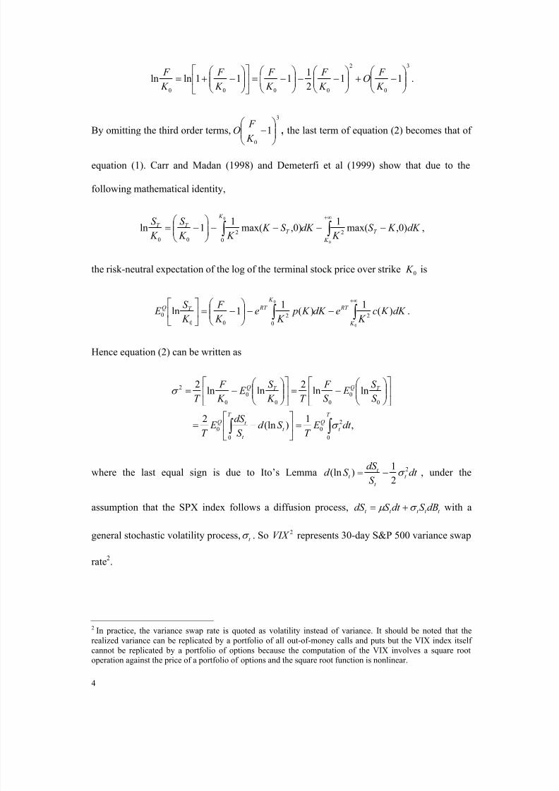
8/4/2019 The Market for Volatility Trading VIX Futures
http://slidepdf.com/reader/full/the-market-for-volatility-trading-vix-futures 5/30
4
3
0
2
0000
112
1111lnln
−+
−−
−=
−+=
K
F O
K
F
K
F
K
F
K
F .
By omitting the third order terms,
3
0
1
−
K
F O , the last term of equation (2) becomes that of
equation (1). Carr and Madan (1998) and Demeterfi et al (1999) show that due to the
following mathematical identity,
∫ ∫ +∞
−−−−
−=
0
0
)0,max(1
)0,max(1
1ln2
0
2
00 K
T
K
T T T dK K S
K dK S K
K K
S
K
S ,
the risk-neutral expectation of the log of the terminal stock price over strike 0 K is
∫ ∫ +∞
−−
−=
0
0
)(1
)(1
1ln2
0
2
00
0
K
RT
K
RT T Q dK K c K
edK K p K
e K
F
K
S E .
Hence equation (2) can be written as
,1
)(ln2
lnln2
lnln2
0
2
0
0
0
0
0
00
0
0
2
∫ ∫ =
−=
−=
−=
T
t
QT
t
t
t Q
T QT Q
dt E T
S d S
dS E
T
S
S E
S
F
T K
S E
K
F
T
σ
σ
where the last equal sign is due to Ito’s Lemma dt S
dS S d t
t
t t
2
2
1)(ln σ −= , under the
assumption that the SPX index follows a diffusion process, t t t t t dBS dt S dS σ µ += with a
general stochastic volatility process, t σ . So 2VIX represents 30-day S&P 500 variance swap
rate2.
2 In practice, the variance swap rate is quoted as volatility instead of variance. It should be noted that therealized variance can be replicated by a portfolio of all out-of-money calls and puts but the VIX index itself cannot be replicated by a portfolio of options because the computation of the VIX involves a square rootoperation against the price of a portfolio of options and the square root function is nonlinear.
8/4/2019 The Market for Volatility Trading VIX Futures
http://slidepdf.com/reader/full/the-market-for-volatility-trading-vix-futures 6/30
5
On March 26, 2004, the newly created CBOE Futures Exchange (CFE) started to trade
an exchange listed volatility product; VIX futures, a futures contract written on the VIX
index. It is cash settled with the VIX. Since VIX is not a traded asset, one cannot replicate a
VIX futures contract using the VIX and a risk free asset. Thus a cost-of-carry relationship
between VIX futures and VIX cannot be established.
Our objective is two fold; First, to use market data to analyse empirically the
relationship between VIX futures prices and VIX, the term structure of VIX futures prices
and to estimate the volatility of VIX futures prices. Second, to find parameter estimates,
using a simple stochastic volatility model, that best describe the empirical relationships and
could possibly be used to price VIX futures and options.
2. Data
In this paper, we use the daily VIX index and VIX futures data provided by the CBOE.
The VIX index data, including open, high, low and close levels, are available from January
2 1990 to the present. The VIX futures data, including open, high, low, close and settle
prices, trading volume and open interest, are available from March 26 2004 to the present.
For each day we have four futures contracts: two near term and two additional months
on the February quarterly cycle. For example, on the first day of the listing, 26 March 2004,
four contracts K4, M4, Q4 and X4 were traded which stand for the following futures
expiration: May, June, August and November 2004 respectively. The first letter indicates
the expiration month followed by the expiration year. The underlying value of the VIX
futures contract is VIX times 10 under the symbol “VXB”
VXB = 10 × VIX . (3)
8/4/2019 The Market for Volatility Trading VIX Futures
http://slidepdf.com/reader/full/the-market-for-volatility-trading-vix-futures 7/30
6
The contract size is $100 times VXB. For example, with a VIX value of 17.33 on 26 March
2004, the VXB would be 173.3 and the contract size would be $17,330. The settlement date
is usually the Wednesday prior to the third Friday of the expiration month.
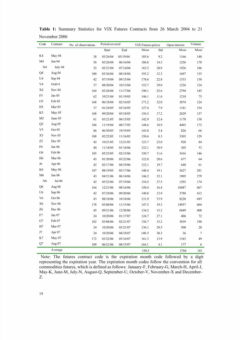
Our empirical study covers the period of two years and eight months from March 16
2004 to November 21 2006, within which there were 34 contract months traded all together.
Table 1 provides a summary statistics of all of them. The average open interest for each
contract is 2784, which corresponds to a market value of 38 million dollars3. The average
daily trading volume for each contract is 181, which corresponds to 2.5 million dollars. The
shortest contract lasted 35 days, while the longest 188 days. The average futures price for
each contract changed from 185.6 for contracts that matured in May 2004 to 164.1 for
contracts that will mature in August 2007 (the average was taken for samples up to the
maturity date or November 21 2006, whichever is earlier), while the VIX level ranged from
17.33 on March 26 2004 to 9.90 on November 21 2006. In general, the market expected
future volatility decreased during this period.
3. Empirical evidence
3.1. The relation between VIX futures and VIX (VXB)
Because the underlying variable of VIX futures, i.e. VXB, is not a traded asset, we are not
able to obtain a simple cost-of-carry relationship, arbitrage free, between the futures price,
T
t F , and its underlying, t VXB . That is,
)( t T r
t
T
t eVXB F −≠ ,
3 Using the average VIX futures prices 135.5, we compute the market value as 135.5 × 100 × 2784 =37,723,200.

8/4/2019 The Market for Volatility Trading VIX Futures
http://slidepdf.com/reader/full/the-market-for-volatility-trading-vix-futures 8/30
7
where r is the interest rate, and T is the maturity. Thus, we have gone to the data to see what
we can learn about the relationship between VIX futures prices and VXB. We use this
relationship to estimate the parameters, in a stochastic volatility model, that could be used to
price volatility derivatives.
There are four futures contracts available on a typical day. For example, on 26 March
2004, we have four kind of VIX futures with maturities, in May, June, August and
November, which corresponds to times to maturity of 53, 80, 142 and 231 days. We
construct 30, 60 and 90-day futures prices by a linear interpolation technique. For example,
the 30-day futures price is computed by using the market data of VXB and May futures on
26 March 2004. The 60-day futures price is computed by using the market data of May and
June futures. The 90-day futures price is computed with June and August futures. We
calculate these fixed time-to-maturity futures price on each day and obtain three time series
of 30-, 60-, and 90-day futures prices. Figure 1 shows the time series of VXB and VIX
futures for three fixed time-to-maturities. Intuitively the four time series are highly
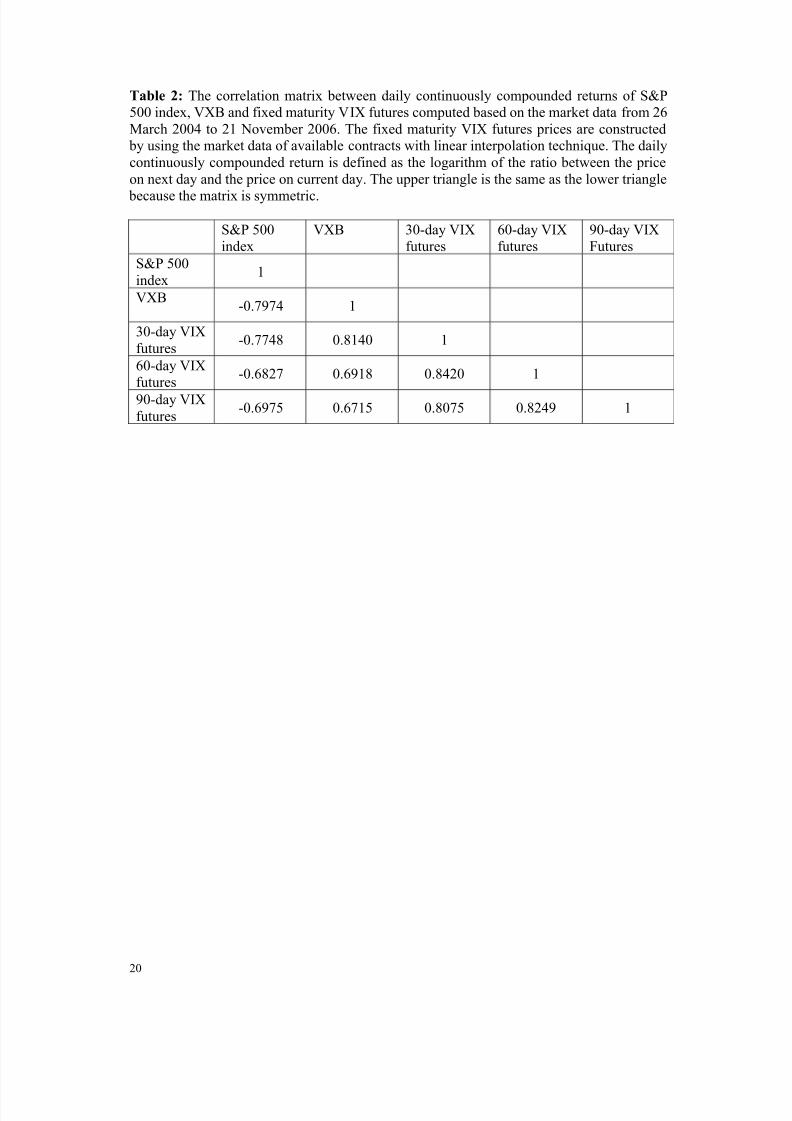
correlated. Table 2 presents the correlation matrix between the returns of S&P 500 index,
VXB and VIX futures. The return is computed as the logarithm of the price relative on two
consecutive ends of day prices. All of the four series are negatively correlated with the S&P
500 index. VXB and VIX futures with three different maturities are almost perfectly
correlated. Figure 1 also shows that the trading volume of VIX futures has been gradually
increasing.
Figure 2 shows the relationship between 30-day VIX futures and VXB for the market
data from 26 March 2004 to 21 November 2006. In general, the VIX futures price is an
increasing function of VXB. The higher the VIX (VXB), the higher is the price of VIX
futures with a given maturity.
8/4/2019 The Market for Volatility Trading VIX Futures
http://slidepdf.com/reader/full/the-market-for-volatility-trading-vix-futures 9/30
8
3.2. The term structure of VIX futures price
Over the period of March 26 2004 to 21 November 2006, the average VXB was 135.5.
The average VIX futures prices were 144.8, 152.8 and 157.8 for 30-, 60- and 90-day
maturities respectively. The term structure of the average VIX futures price is upward
sloping, which is demonstrated graphically in Figure 3.
The upward sloping VIX futures term structure indicates that the current level of
volatility is relatively low compared with the long-term mean level and that the volatility is
increasing to the long-term high level.
3.3. The volatility of VXB and VIX futures
With the time series of VXB and fixed maturity VIX futures price, we compute the
standard deviation of daily log price (index) relatives to obtain estimates of the volatility of
these four series, assuming that these series follow a lognormal process. During the two year
period of our study we estimated the volatility of VXB to be 84.4%, while the volatilities of
VIX futures price are 35.7%, 30.0% and 25.8% for 30, 60 and 90 day maturities
respectively. The longer the maturity, the lower is the volatility of volatility. Figure 4 shows
the volatility of VXB and fixed maturity VIX futures price. The term structure of VIX
futures volatility is downward sloping.
The phenomenon of downward sloping VIX futures volatility is consistent with the
mean-reverting feature of the volatility. Since the long-term volatility approaches to a fixed
level, long-tenor VIX futures should be less volatile than short-tenor ones.
8/4/2019 The Market for Volatility Trading VIX Futures
http://slidepdf.com/reader/full/the-market-for-volatility-trading-vix-futures 10/30
9
4. A Theoretical Model of VIX Futures price
4.1. VIX futures price
We now use a simple theoretical model to price the futures contracts using parameter
estimates obtained from market data. We then test the extent to which model prices can
explain market prices.
In the physical measure, the SPX index, t S , is assumed to follow Heston (1993)
stochastic variance model
P
t t t t t dBS V dt S dS 1+= µ ,
P
t t V t
P P
t dBV dt V dV 2)( σ θ κ +−= ,
where µ is the expected return, P θ is long-term mean level of the instantaneous variance,
P κ is the mean-reverting speed of the variance, V σ measures the volatility of variance,
P
t dB1 and P
t dB2 are increments of two Brownian motions that describe the random noises in
SPX index return and variance. They are assumed to be correlated with a constant
coefficient, ρ .
By changing probability measure from P to Q as follows,
dt V
r dBdB
t
Q
t
P
t
−−=µ
11 , dt V dBdB t
V
Q
t
P
t σ
λ −= 22 ,
where r is the risk-free rate, and λ is the market price of variance risk, we obtain the
dynamics of the SPX index in the risk-neutral measure
Q
t t t t t dBS V dt rS dS 1+= ,
Q
t t V t
P P P
t dBV dt V dV 2])([ σ λ κ θ κ ++−= ,
8/4/2019 The Market for Volatility Trading VIX Futures
http://slidepdf.com/reader/full/the-market-for-volatility-trading-vix-futures 11/30
10
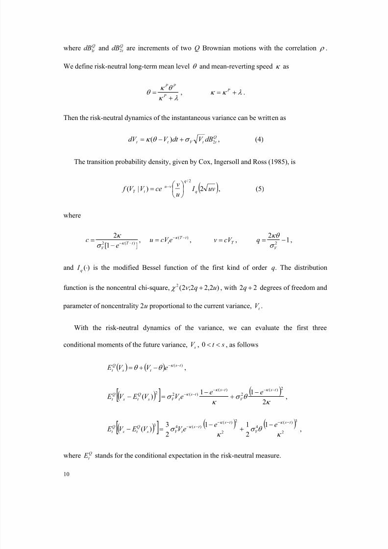
where Q
t dB1 and Q
t dB2 are increments of two Q Brownian motions with the correlation ρ .
We define risk-neutral long-term mean level θ and mean-reverting speed κ as
λ κ
θ κ θ
+=
P
P P
, λ κ κ += P .
Then the risk-neutral dynamics of the instantaneous variance can be written as
Q
t t V t t dBV dt V dV 2)( σ θ κ +−= , (4)
The transition probability density, given by Cox, Ingersoll and Ross (1985), is
( )uv I u
v
ceV V f q
q
vu
t T 2)|(
2/
= −−
, (5)
where
,]1[
2)(2 t T
V ec
−−−=
κ σ
κ )( t T
t ecV u −−= κ , T cV v = , 12
2−=
V
qσ
κθ ,
and )(⋅q I is the modified Bessel function of the first kind of order q. The distribution
function is the noncentral chi-square, )2,22;2(2
uqv + χ , with 22 +q degrees of freedom and
parameter of noncentrality 2u proportional to the current variance, t V .
With the risk-neutral dynamics of the variance, we can evaluate the first three
conditional moments of the future variance, sV , st <<0 , as follows
( ) ( ) )( t s
t s
Q
t eV V E −−−+= κ θ θ ,
( )[ ] ( )κ
θ σ κ
σ κ κ
κ
2
11)(
2)(2
)()(22
t s
V
t st s
t V s
Q
t s
Q
t
eeeV V E V E
−−−−−− −
+−
=− ,
( )[ ] ( ) ( )2
3)(4
2
2)()(43 1
2
11
2
3)(
κ θ σ
κ σ
κ κ κ
t s
V
t st s
t V s
Q
t s
Q
t
eeeV V E V E
−−−−−− −
+−
=− ,
where Q
t E stands for the conditional expectation in the risk-neutral measure.
8/4/2019 The Market for Volatility Trading VIX Futures
http://slidepdf.com/reader/full/the-market-for-volatility-trading-vix-futures 12/30
11
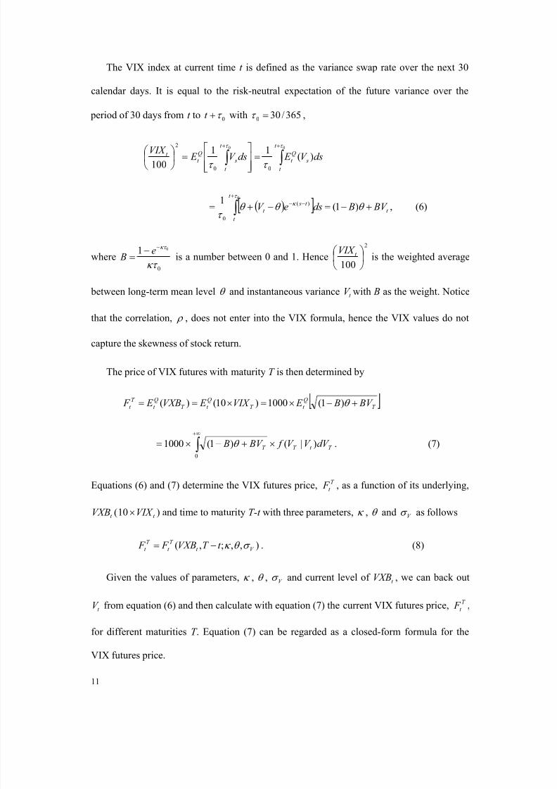
The VIX index at current time t is defined as the variance swap rate over the next 30
calendar days. It is equal to the risk-neutral expectation of the future variance over the
period of 30 days from t to 0τ +t with 365/300 =τ ,
∫ ∫ ++
=
=
00
)(11
100 00
2 τ τ
τ τ
t
t
s
Q
t
t
t
s
Q
t t dsV E dsV E
VIX
( )[ ] t
t
t
t s
t BV BdseV +−=−+= ∫ +
−− θ θ θ τ
τ
κ )1(1 0
)(
0
, (6)
where0
01
κτ
κτ −−=
e B is a number between 0 and 1. Hence
2
100
t VIX is the weighted average
between long-term mean level θ and instantaneous variance t V with B as the weight. Notice
that the correlation, ρ , does not enter into the VIX formula, hence the VIX values do not
capture the skewness of stock return.
The price of VIX futures with maturity T is then determined by
T
Q
t T
Q
t T
Q
t
T
t BV B E VIX E VXB E F +−×=×== θ )1(1000)10()(
T t T T dV V V f BV B )|()1(10000
×+−×= ∫ +∞
θ . (7)
Equations (6) and (7) determine the VIX futures price, T
t F , as a function of its underlying,
t VXB ( t VIX ×10 ) and time to maturity T-t with three parameters, κ , θ and V σ as follows
),,;,( V t
T
t
T
t t T VXB F F σ θ κ −= . (8)
Given the values of parameters, κ , θ , V σ and current level of t VXB , we can back out
t V from equation (6) and then calculate with equation (7) the current VIX futures price, T
t F ,
for different maturities T . Equation (7) can be regarded as a closed-form formula for the
VIX futures price.
8/4/2019 The Market for Volatility Trading VIX Futures
http://slidepdf.com/reader/full/the-market-for-volatility-trading-vix-futures 13/30
12
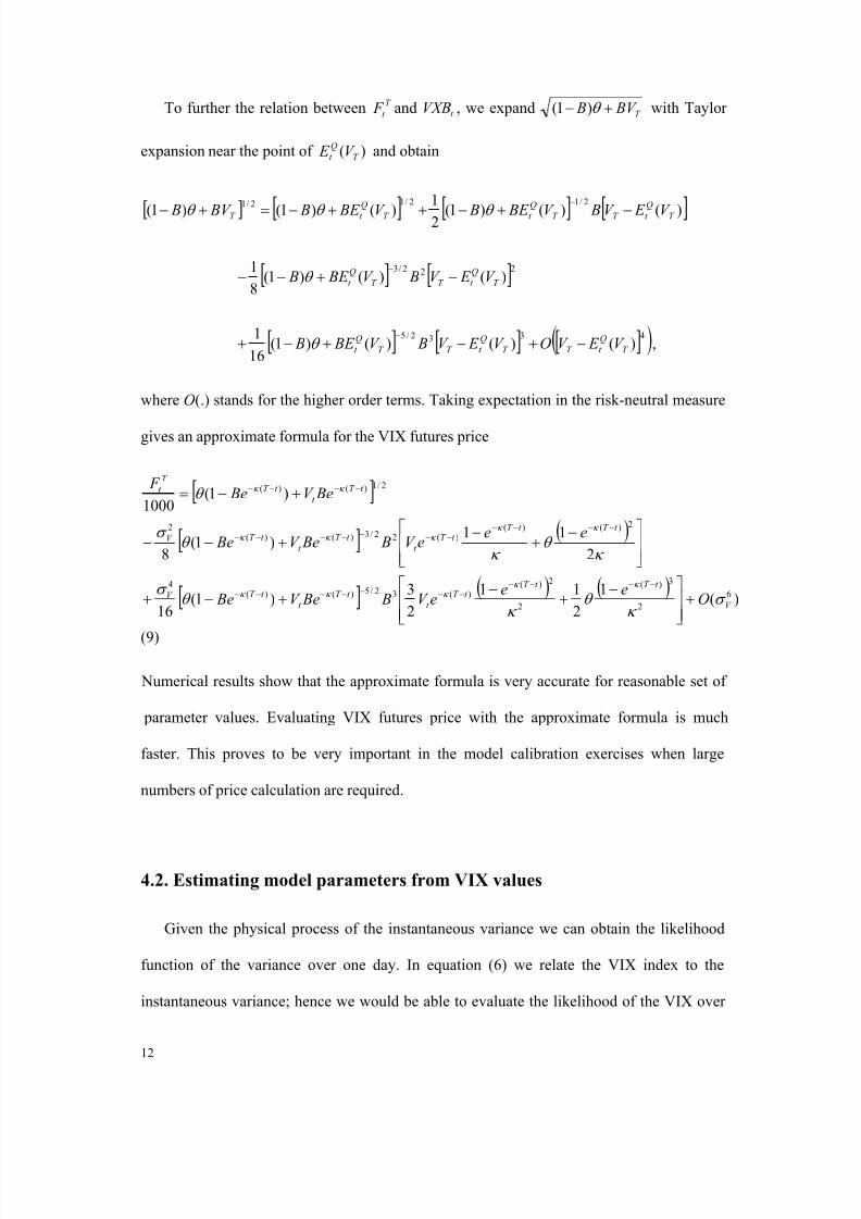
To further the relation between T
t F and t VXB , we expand T BV B +− θ )1( with Taylor
expansion near the point of )( T
Q
t V E and obtain
[ ] [ ] [ ] [ ])()()1(2
1
)()1()1(
2/12/12/1
T
Q
t T T
Q
t T
Q
t T V E V BV BE BV BE B BV B −+−++−=+−
−
θ θ θ
[ ] [ ]222/3)()()1(
8
1T
Q
t T T
Q
t V E V BV BE B −+−−−
θ
[ ] [ ] [ ]( )4332/5)()()()1(
16
1T
Q
t T T
Q
t T T
Q
t V E V OV E V BV BE B −+−+−+−
θ ,
where O(.) stands for the higher order terms. Taking expectation in the risk-neutral measure
gives an approximate formula for the VIX futures price
[ ]
[ ] ( )
[ ] ( ) ( ))(
1
2
11
2
3)1(
16
2
11)1(
8
)1(1000
6
2
3)(
2
2)()(32/5)()(
4
2)()()(22/3)()(
2
2/1)()(
V
t T t T t T
t
t T
t
t T V
t T t T t T
t
t T
t
t T V
t T
t
t T T
t
Oee
eV B BeV Be
eeeV B BeV Be
BeV Be F
σ κ
θ κ
θ σ
κ θ
κ θ
σ
θ
κ κ κ κ κ
κ κ κ κ κ
κ κ
+
−+
−+−+
−+
−+−−
+−=
−−−−−−−−−−−
−−−−−−−−−−−
−−−−
(9)
Numerical results show that the approximate formula is very accurate for reasonable set of
parameter values. Evaluating VIX futures price with the approximate formula is much
faster. This proves to be very important in the model calibration exercises when large
numbers of price calculation are required.
4.2. Estimating model parameters from VIX values
Given the physical process of the instantaneous variance we can obtain the likelihood
function of the variance over one day. In equation (6) we relate the VIX index to the
instantaneous variance; hence we would be able to evaluate the likelihood of the VIX over
8/4/2019 The Market for Volatility Trading VIX Futures
http://slidepdf.com/reader/full/the-market-for-volatility-trading-vix-futures 14/30
13
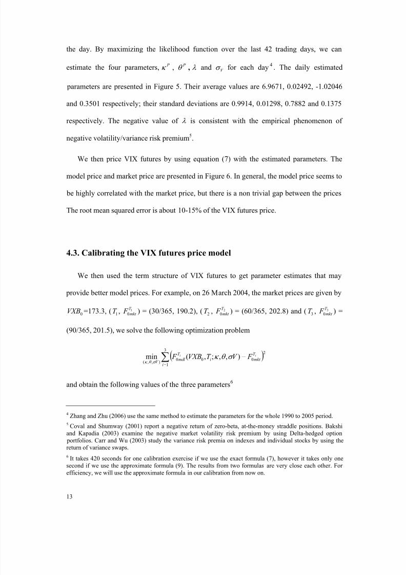
the day. By maximizing the likelihood function over the last 42 trading days, we can
estimate the four parameters, P κ , P θ , λ and V σ for each day 4 . The daily estimated
parameters are presented in Figure 5. Their average values are 6.9671, 0.02492, -1.02046
and 0.3501 respectively; their standard deviations are 0.9914, 0.01298, 0.7882 and 0.1375
respectively. The negative value of λ is consistent with the empirical phenomenon of
negative volatility/variance risk premium5.
We then price VIX futures by using equation (7) with the estimated parameters. The
model price and market price are presented in Figure 6. In general, the model price seems to
be highly correlated with the market price, but there is a non trivial gap between the prices
The root mean squared error is about 10-15% of the VIX futures price.
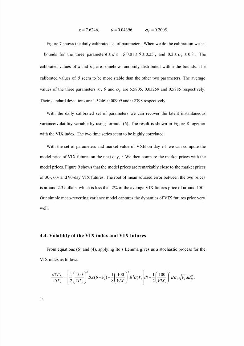
4.3. Calibrating the VIX futures price model
We then used the term structure of VIX futures to get parameter estimates that may
provide better model prices. For example, on 26 March 2004, the market prices are given by
0VXB =173.3, ( 1T , 1
0
T
mkt F ) = (30/365, 190.2), ( 2T , 2
0
T
mkt F ) = (60/365, 202.8) and ( 3T , 3
0
T
mkt F ) =
(90/365, 201.5), we solve the following optimization problem
( )∑=
−3
1
2
000),,(
),,;,(mini
T
mkt i
T
mdl V
ii F V T VXB F σ θ κ σ θ κ
and obtain the following values of the three parameters6
4 Zhang and Zhu (2006) use the same method to estimate the parameters for the whole 1990 to 2005 period.
5 Coval and Shumway (2001) report a negative return of zero-beta, at-the-money straddle positions. Bakshiand Kapadia (2003) examine the negative market volatility risk premium by using Delta-hedged option portfolios. Carr and Wu (2003) study the variance risk premia on indexes and individual stocks by using thereturn of variance swaps.
6 It takes 420 seconds for one calibration exercise if we use the exact formula (7), however it takes only one
second if we use the approximate formula (9). The results from two formulas are very close each other. For efficiency, we will use the approximate formula in our calibration from now on.
8/4/2019 The Market for Volatility Trading VIX Futures
http://slidepdf.com/reader/full/the-market-for-volatility-trading-vix-futures 15/30
14
=κ 7.6246, =θ 0.04396, =V σ 0.2005.
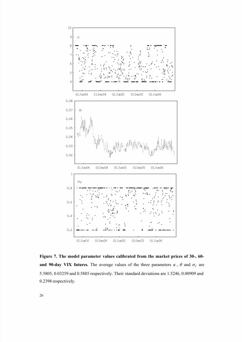
Figure 7 shows the daily calibrated set of parameters. When we do the calibration we set
bounds for the three parameters 84 ≤≤ κ , 25.001.0 ≤≤ θ , and 8.02.0 ≤≤ V σ . The
calibrated values of κ and V σ are somehow randomly distributed within the bounds. The
calibrated values of θ seem to be more stable than the other two parameters. The average
values of the three parameters κ , θ and V σ are 5.5805, 0.03259 and 0.5885 respectively.
Their standard deviations are 1.5246, 0.00909 and 0.2398 respectively.
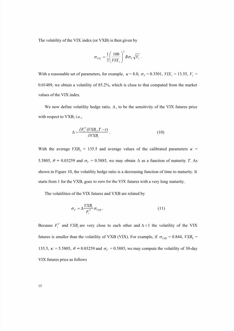
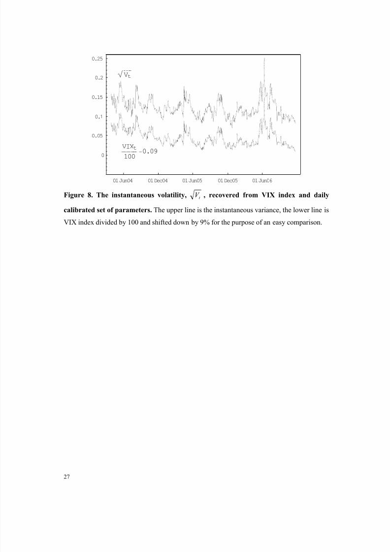
With the daily calibrated set of parameters we can recover the latent instantaneous
variance/volatility variable by using formula (6). The result is shown in Figure 8 together
with the VIX index. The two time series seem to be highly correlated.
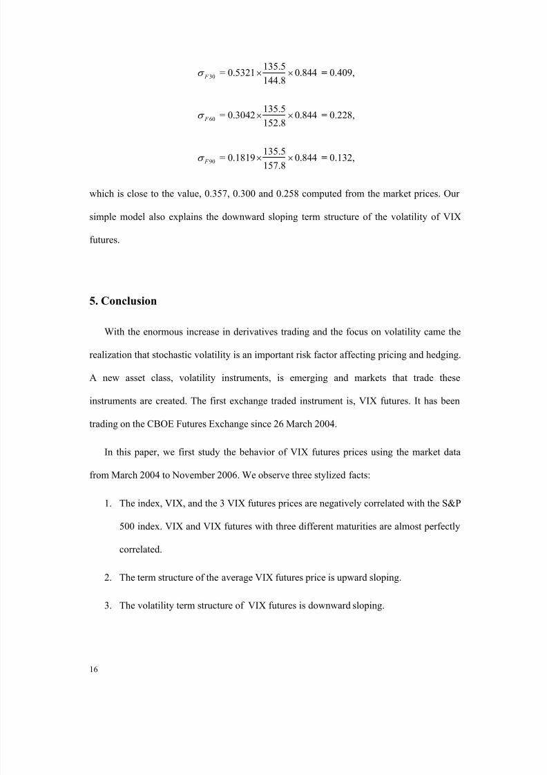
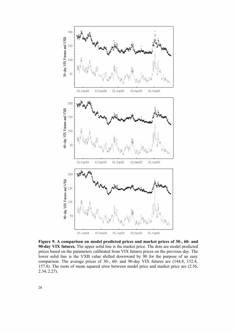
With the set of parameters and market value of VXB on day t -1 we can compute the
model price of VIX futures on the next day, t . We then compare the market prices with the
model prices. Figure 9 shows that the model prices are remarkably close to the market prices
of 30-, 60- and 90-day VIX futures. The root of mean squared error between the two prices
is around 2.3 dollars, which is less than 2% of the average VIX futures price of around 150.
Our simple mean-reverting variance model captures the dynamics of VIX futures price very
well.
4.4. Volatility of the VIX index and VIX futures
From equations (6) and (4), applying Ito’s Lemma gives us a stochastic process for the
VIX index as follows
Q
t t V
t
t V
t
t
t t
t dBV BVIX
dt V BVIX
V BVIX VIX
dVIX 2
2
22
42
100
2
1100
8
1)(
100
2
1σ σ θ κ
+
−−
= .
8/4/2019 The Market for Volatility Trading VIX Futures
http://slidepdf.com/reader/full/the-market-for-volatility-trading-vix-futures 16/30
15
The volatility of the VIX index (or VXB) is then given by
t V t
VIX V BVIX σ σ
2
100
2
1
= .
With a reasonable set of parameters, for example, κ = 8.0, V σ = 0.3501, t VIX = 13.55, t V =
0.01489, we obtain a volatility of 85.2%, which is close to that computed from the market
values of the VIX index.
We now define volatility hedge ratio, ∆ , to be the sensitivity of the VIX futures price
with respect to VXB, i.e.,
t
t
T
t
VXB
t T VXB F
∂
−∂=∆
),(. (10)
With the average 0VXB = 135.5 and average values of the calibrated parameters κ =
5.5805, θ = 0.03259 and V σ = 0.5885, we may obtain ∆ as a function of maturity T . As
shown in Figure 10, the volatility hedge ratio is a decreasing function of time to maturity. It
starts from 1 for the VXB, goes to zero for the VIX futures with a very long maturity.
The volatilities of the VIX futures and VXB are related by
VXBT
t
t F
F
VXBσ σ ∆= . (11)
Because T
t F and t VXB are very close to each other and 1<∆ the volatility of the VIX
futures is smaller than the volatility of VXB (VIX). For example, if VXBσ = 0.844, 0VXB =
135.5, κ = 5.5805, θ = 0.03259 and V σ = 0.5885, we may compute the volatility of 30-day
VIX futures price as follows
8/4/2019 The Market for Volatility Trading VIX Futures
http://slidepdf.com/reader/full/the-market-for-volatility-trading-vix-futures 17/30
16
30 F σ = 0.5321 844.08.144
5.135×× = 0.409,
60 F σ = 0.3042 844.08.152
5.135×× = 0.228,
90 F σ = 0.1819 844.08.157
5.135×× = 0.132,
which is close to the value, 0.357, 0.300 and 0.258 computed from the market prices. Our
simple model also explains the downward sloping term structure of the volatility of VIX
futures.
5. Conclusion
With the enormous increase in derivatives trading and the focus on volatility came the
realization that stochastic volatility is an important risk factor affecting pricing and hedging.
A new asset class, volatility instruments, is emerging and markets that trade these
instruments are created. The first exchange traded instrument is, VIX futures. It has been
trading on the CBOE Futures Exchange since 26 March 2004.
In this paper, we first study the behavior of VIX futures prices using the market data
from March 2004 to November 2006. We observe three stylized facts:
1. The index, VIX, and the 3 VIX futures prices are negatively correlated with the S&P
500 index. VIX and VIX futures with three different maturities are almost perfectly
correlated.
2. The term structure of the average VIX futures price is upward sloping.
3. The volatility term structure of VIX futures is downward sloping.
8/4/2019 The Market for Volatility Trading VIX Futures
http://slidepdf.com/reader/full/the-market-for-volatility-trading-vix-futures 18/30
17
The first fact is not surprising. Traders often take long position in volatility derivatives to
hedge the risk in stock position. The second fact shows that the long term mean level of
volatility is higher than the current level. The third observation is not well-known.
In the second part of the paper we use a simple mean-reverting variance model to
establish the theoretical relationship between VIX futures prices and its underlying spot
index. Using the variance parameters calibrated from our model with the market data at t-1,
we can price VIX futures at time t conditional on VIX at time t . An empirical study over the
whole sample period shows that our model provides prices that are very close to the market
prices. The root mean squared error between the market and model prices is around 2.3
dollars, which is less than 2% of the average VIX futures price of around 150. Our simple
mean-reverting variance model captures the dynamics of VIX futures price very well.
References:
1. Bakshi, Gurdip, and Nikunji Kapadia, 2003, Delta-hedged gains and the negative market
volatility risk premium, Review of Financial Studies 16, 527-566.
2. Brenner, Menachem, and Dan Galai, 1989, New Financial Instruments for Hedging
Changes in Volatility, Financial Analyst Journal , July/August, 61-65.
3. Carr, Peter, and Dilip Madan, 1998, Towards a theory of volatility trading. In Robert
Jarrow (Ed.), Volatility estimation techniques for pricing derivatives, London: Risk
Books, pp. 417-427.
4. Carr, Peter, and Liuren Wu, 2003, Variance risk premia, Working paper, City University
of New York and Bloomberg L. P.
5. Carr, Peter, and Liuren Wu, 2006, A tale of two indices, Journal of Derivatives 13, 13-
29.
8/4/2019 The Market for Volatility Trading VIX Futures
http://slidepdf.com/reader/full/the-market-for-volatility-trading-vix-futures 19/30
18
6. Corrado, Charles J., and Thomas W. Miller, Jr., 2005, The forecast quality of CBOE
implied volatility indexes, Journal of Futures Markets 25, 339-373.
7. Coval, Joshua D., and Tyler Shumway, 2001, Expected option returns, Journal of
Finance 56, 983-1009.
8. Cox, John C., Jonathan E. Ingersoll, Jr., and Stephen A. Ross, 1985, A theory of the
term structure of interest rates, Econometrica 53, 385-407.
9. Demeterfi, Kresimir, Emanuel Derman, Michael Kamal, and Joseph Zou, 1999, A guide
to volatility and variance swaps, Journal of Derivatives 6, 9-32.
10. Heston, Steven L., 1993, A closed-form solution for options with stochastic volatility
with applications to bond and currency options, Review of Financial Studies 6, 327-343.
11. Merton, Robert C., 1973, Theory of Rational Option Pricing. Bell Journal of Economics
and Management Science 4 , 141-183.
12. Zhang, Jin E., and Yingzi Zhu, 2006, VIX Futures, Journal of Futures Markets 26, 521-
531.
8/4/2019 The Market for Volatility Trading VIX Futures
http://slidepdf.com/reader/full/the-market-for-volatility-trading-vix-futures 20/30
19
Table 1: Summary Statistics for VIX Futures Contracts from 26 March 2004 to 21
November 2006
Code Contract No. of observations Period covered VIX Futures prices Open interest Volume
Start End Mean Std Mean Mean
K4 May 04 38 03/26/04 05/19/04 185.6 9.2 1166 148
M4 Jun 04 56 03/26/04 06/16/04 186.8 14.3 1256 170
N4 July 04 35 05/21/04 07/14/04 163.5 30.9 1926 186
Q4 Aug 04 100 03/26/04 08/18/04 193.2 12.3 1697 135
U4 Sep 04 42 07/19/04 09/15/04 178.6 22.8 1533 158
V4 Oct0 4 37 08/20/04 10/13/04 152.7 29.0 1226 124
X4 Nov 04 164 03/26/04 11/17/04 190.1 25.6 2794 145
F5 Jan 05 62 10/21/04 01/19/05 146.1 11.6 1210 75
G5 Feb 05 168 06/18/04 02/16/05 171.2 32.0 3074 124
H5 Mar 05 37 01/24/05 03/16/05 127.4 7.9 1181 154
K5 May 05 168 09/20/04 05/18/05 156.5 17.2 2629 157
M5 June 05 61 03/21/05 06/15/05 142.9 12.4 1178 138Q5 Aug 05 186 11/19/04 08/17/05 148.6 18.9 4403 172
V5 Oct 05 86 06/20/05 10/19/05 143.0 5.4 826 66
X5 Nov 05 188 02/22/05 11/16/05 150.6 8.3 3303 129
Z5 Dec 05 42 10/21/05 12/21/05 123.7 23.0 928 84
F6 Jan 06 40 11/18/05 01/18/06 122.1 20.9 305 52
G6 Feb 06 185 05/23/05 02/15/06 150.7 11.6 3416 146
H6 Mar 06 43 01/20/06 03/22/06 122.8 20.6 677 64
J6 Apr 06 42 02/17/06 04/19/06 122.1 19.7 648 61
K6 May 06 187 08/19/05 05/17/06 148.4 19.1 5627 281
M6 Jun 06 43 04/21/06 06/14/06 146.2 32.1 1905 279
N6 Jul 06 42 05/22/06 07/19/06 154.5 27.5 1293 174
Q6 Aug 06 164 12/21/06 08/16/06 150.4 16.4 10487 467
U6 Sep 06 42 07/24/06 09/20/06 140.8 12.9 3788 412
V6 Oct 06 43 08/18/06 10/18/06 131.9 23.9 8220 685
X6 Nov 06 178 03/08/06 11/15/06 147.5 19.3 14957 604
Z6 Dec 06 45 09/21/06 12/20/06 134.2 15.2 6849 408
F7 Jan 07 24 10/20/06 01/17/07 124.7 27.1 406 72
G7 Feb 07 182 03/08/06 02/21/07 156.7 15.2 3839 190
H7 Mar 07 24 10/20/06 03/21/07 136.1 29.5 508 28
J7 Apr 07 24 10/20/06 04/18/07 140.5 30.3 36 7
K7 May 07 172 03/22/06 05/16/07 161.3 13.9 1183 49Q7 Aug 07 109 06/21/06 08/15/07 164.1 4.1 177 6
Average 150.5 2784 181
Note: The futures contract code is the expiration month code followed by a digitrepresenting the expiration year. The expiration month codes follow the convention for allcommodities futures, which is defined as follows: January-F, February-G, March-H, April-J,May-K, June-M, July-N, August-Q, September-U, October-V, November-X and December-Z.
8/4/2019 The Market for Volatility Trading VIX Futures
http://slidepdf.com/reader/full/the-market-for-volatility-trading-vix-futures 21/30
20
Table 2: The correlation matrix between daily continuously compounded returns of S&P500 index, VXB and fixed maturity VIX futures computed based on the market data from 26March 2004 to 21 November 2006. The fixed maturity VIX futures prices are constructed
by using the market data of available contracts with linear interpolation technique. The dailycontinuously compounded return is defined as the logarithm of the ratio between the priceon next day and the price on current day. The upper triangle is the same as the lower triangle
because the matrix is symmetric.
S&P 500index
VXB 30-day VIXfutures
60-day VIXfutures
90-day VIXFutures
S&P 500index
1
VXB-0.7974 1
30-day VIXfutures
-0.7748 0.8140 1
60-day VIXfutures
-0.6827 0.6918 0.8420 1
90-day VIXfutures
-0.6975 0.6715 0.8075 0.8249 1
8/4/2019 The Market for Volatility Trading VIX Futures
http://slidepdf.com/reader/full/the-market-for-volatility-trading-vix-futures 22/30
21
0
50
100
150
200
250
300
2 0 0 4 - 3 - 2 6
2 0 0 4 - 5 - 2 6
2 0 0 4 - 7 - 2 6
2 0 0 4 - 9 - 2 6
2 0 0 4 - 1 1 - 2 6
2 0 0 5 - 1 - 2 6
2 0 0 5 - 3 - 2 6
2 0 0 5 - 5 - 2 6
2 0 0 5 - 7 - 2 6
2 0 0 5 - 9 - 2 6
2 0 0 5 - 1 1 - 2 6
2 0 0 6 - 1 - 2 6
2 0 0 6 - 3 - 2 6
2 0 0 6 - 5 - 2 6
2 0 0 6 - 7 - 2 6
2 0 0 6 - 9 - 2 6
Trading VolumeVXB30-day VIX Futures60-day VIX Futures90-day VIX Futures
Figure 1. VXB and VIX futures price with three fixed time-to-maturities between 26
March 2004 and 21 November 2006. The VXB time series is from the CBOE. The fixedmaturity VIX futures prices are constructed by using the market data of available contracts
with linear interpolation technique. The bar chart shows the trading volume (normalized by
100 contracts) of futures of all maturity on the day.
0
50
100
150
200
250
0 50 100 150 200 250 300
VXB
3 0 - d a y V I X F u t u r e s
Figure 2. The relation between 30-day VIX futures and VXB (March 26 2004 – 21
November 2006). The VXB time series is from the CBOE. The 30-day VIX futures prices
are constructed by using the market data of available contracts with linear interpolation
technique.
8/4/2019 The Market for Volatility Trading VIX Futures
http://slidepdf.com/reader/full/the-market-for-volatility-trading-vix-futures 23/30
22
(90,157.8)
(60,152.8)
(30,144.8)
(0,135.5)
120
125
130
135
140
145
150
155
160
0 30 60 90
Time to Maturity
A v e r a g e V I X
F u t u r e s P r i c e
Figure 3. The term structure of average VIX futures price. The average VIX futures price is computed based on the fixed maturity data from 26 March 2004 to 21 November
2006. The fixed maturity VIX futures prices are constructed by using the market data of
available contracts with linear interpolation technique.
0.844
0.3570.300
0.258
0.0
0.1
0.2
0.3
0.4
0.5
0.6
0.7
0.8
0.9
0 30 60 90Time to Maturity
V o l a t i l i t y
o f V I X F
u t u r e s P r i c e
Figure 4. The annualized volatility of VIX futures price. The annualized volatility is
computed based on the fixed maturity data from 26 March 2004 to 21 November 2006. The
fixed maturity VIX futures prices are constructed by using the market data of available
contracts with linear interpolation technique.

8/4/2019 The Market for Volatility Trading VIX Futures
http://slidepdf.com/reader/full/the-market-for-volatility-trading-vix-futures 24/30
23
01Jun04 01Dec04 01Jun05 01Dec05 01Jun06
4
5
6
7
8
9
10
κP
01Jun04 01Dec04 01Jun05 01Dec05 01Jun06
0.02
0.04
0.06
0.08 θP
01Jun04 01Dec04 01Jun05 01Dec05 01Jun06
-3
-2
-1
0
1
λ
8/4/2019 The Market for Volatility Trading VIX Futures
http://slidepdf.com/reader/full/the-market-for-volatility-trading-vix-futures 25/30
24
01Jun04 01Dec04 01Jun05 01Dec05 01Jun06
0.2
0.4
0.6
0.8
1
σ V
Figure 5. The variance parameters estimated from the historical VIX index of the last
42 trading days. The average values of the estimated four parameters P κ , P
θ , λ and V σ
are 6.9671, 0.02492, -1.02046 and 0.3501 respectively. Their standard deviations are
0.9914, 0.01298, 0.7882 and 0.1375 respectively.
8/4/2019 The Market for Volatility Trading VIX Futures
http://slidepdf.com/reader/full/the-market-for-volatility-trading-vix-futures 26/30
25
01Jun04 01Dec04 01Jun05 01Dec05 01Jun06
50
100
150
200
250
0 3 -
y a d
X I V
s e r
u t u F
e c i r P
d n a
B X V
01Jun04 01Dec04 01Jun05 01Dec05 01Jun06
50
100
150
200
250
0 6 -
y a d
X I V
s e r u t u F
e c i r P
d n a
B X V
01Jun04 01Dec04 01Jun05 01Dec05 01Jun06
50
100
150
200
250
0 9 -
y a d
X I V
s e r u t u F
e c i r P
d n a
B
X V
Figure 6. A comparison of model predicted prices and market prices of 30-, 60- and 90-
day VIX futures. The upper solid line is the market price. The dots are model predicted prices based on the parameters estimated from the VIX index of the last 42 trading days.The lower solid line is the VXB value shifted downward by 90 for the purpose of an easycomparison. The average prices of 30-, 60- and 90-day VIX futures are (144.8, 152.8,157.8). The roots of mean squared error between model predicted price and market price are(14.89, 21.97, 26.18).
8/4/2019 The Market for Volatility Trading VIX Futures
http://slidepdf.com/reader/full/the-market-for-volatility-trading-vix-futures 27/30
26
01Jun04 01Dec04 01Jun05 01Dec05 01Jun06
4
5
6
7
8
9
10
κ
01Jun04 01Dec04 01Jun05 01Dec05 01Jun06
0.02
0.03
0.04
0.05
0.06
0.07
0.08
θ
01Jun04 01Dec04 01Jun05 01Dec05 01Jun06
0.2
0.4
0.6
0.8
1
σ V
Figure 7. The model parameter values calibrated from the market prices of 30-, 60-
and 90-day VIX futures. The average values of the three parameters κ , θ and V σ are
5.5805, 0.03259 and 0.5885 respectively. Their standard deviations are 1.5246, 0.00909 and
0.2398 respectively.
8/4/2019 The Market for Volatility Trading VIX Futures
http://slidepdf.com/reader/full/the-market-for-volatility-trading-vix-futures 28/30
27
01Jun04 01Dec04 01Jun05 01Dec05 01Jun06
0
0.05
0.1
0.15
0.2
0.25
è ! ! !!Vt
VIXt
100−0.09
Figure 8. The instantaneous volatility, t V , recovered from VIX index and daily
calibrated set of parameters. The upper line is the instantaneous variance, the lower line is
VIX index divided by 100 and shifted down by 9% for the purpose of an easy comparison.
8/4/2019 The Market for Volatility Trading VIX Futures
http://slidepdf.com/reader/full/the-market-for-volatility-trading-vix-futures 29/30
28
01Jun04 01Dec04 01Jun05 01Dec05 01Jun06
50
100
150
200
0 3 -
y a d
X I V
s e r u t u F
d n a
B X V
01Jun04 01Dec04 01Jun05 01Dec05 01Jun06
50
100
150
200
0 6 -
y a d
X I V
s e r u t u F
d n a
B X V
01Jun04 01Dec04 01Jun05 01Dec05 01Jun06
50
100
150
200
0 9 -
y a d
X I V
s e r u t u F
d n a
B X V
Figure 9. A comparison on model predicted prices and market prices of 30-, 60- and
90-day VIX futures. The upper solid line is the market price. The dots are model predicted prices based on the parameters calibrated from VIX futures prices on the previous day. Thelower solid line is the VXB value shifted downward by 90 for the purpose of an easycomparison. The average prices of 30-, 60- and 90-day VIX futures are (144.8, 152.8,157.8). The roots of mean squared error between model price and market price are (2.56,2.34, 2.27).

8/4/2019 The Market for Volatility Trading VIX Futures
http://slidepdf.com/reader/full/the-market-for-volatility-trading-vix-futures 30/30
0 20 40 60 80
Time to maturity HdayL
0.2
0.4
0.6
0.8
1
e g d e H
o i t a r
Figure 10. The volatility hedge ratio as a function of time to maturity. 0VXB = 135.5,
the set of parameters is taken to be the average calibrated values κ = 5.5805, θ = 0.03259
and V σ = 0.5885.