MÉTODOS DE COMPUTACIÓN EN FÍSICA DE LA MATERIA CONDENSADA

Máster en Física de la Materia Condensada y Nanotecnología

Curso 2010-2011

Rafael Delgado Buscalioni

Métodos aplicados a Mecánica Clásica

1. Introduction

2. Monte Carlo (MC)

3. Molecular Dynamics (MD)

4. Langevin Dynamics (thermostats)

5. Brownian Dynamics (colloids, polymers in solvent)

6. Hydro-Dynamics at mesoscales

Course material on the following web page:

http://www.uam.es/otros/fmcyn/MetodosComputacionales.html

Reference books

Molecular Dynamics(Equlibrium and non-equilibrium)Monte Carlo, Brownian Dynamics, etc.

Monte CarloFree Energy, etc..

Understanding Molecular SimulationsDaan Frenkel and Berend SmitAcademic Press (second Edition) (2002)

Computer simulations of LiquidsM.P Allen and D.J TildesleyOxford Science Publi. (1987)

Good

Bad...

...leads to Desperado Coding

How to start a code

Cool

distribution function...

... and its corresponding HISTOGRAM

The Monte Carlo Method

(IMPORTANCE SAMPLING)

.

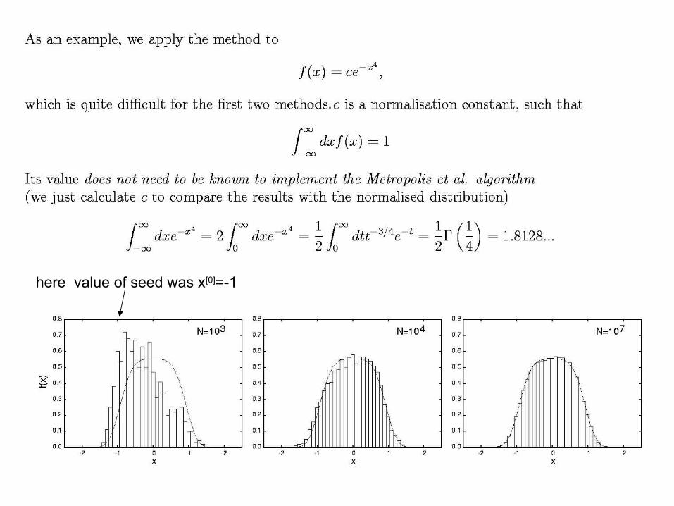
here value of seed was x[0]=-1

The Metropolis Method

Objetive: sample a system whose probability of being in configuration “c” is N(c)

How: Metropolis is based on an importance-weighted random walk:Visited configurations: “c=o” means old config

“c=n” means new configTransition probability: T(o,n).

Along the walk(s) the number of times any “o” is visited is m(o).Thus, we want: m(o) proportional to N(o)

Detailed balance (sample without bias) N(o) T(o,n)=N(n)T(n,o)

Construction of T.Probability of trial from o to n: try(o,n)Probability of accept that trial: acc(o,n)Indeed, T(o,n)=try(o,n) acc(o,n)

Metropolis choice for try: try(o,n)=try(n,o) symmetricDetailed balance: N(o) acc(o,n)=N(n) acc(n,o)i.e, acc(o,n)/acc(n,o) = N(n)/N(o)

Metropolis choice for acc: acc(o,n)= N(n)/N(o) if N(n)<N(o) (visiting less probable config.)acc(o,n)= 1 if N(n)>N(o) (accept if n is more populated)

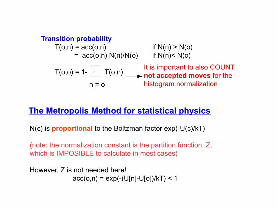
The Metropolis Method for statistical physics

N(c) is proportional to the Boltzman factor exp(-U(c)/kT)

(note: the normalization constant is the partition function, Z,which is IMPOSIBLE to calculate in most cases)

However, Z is not needed here! acc(o,n) = exp(-(U[n]-U[o])/kT) < 1

Transition probabilityT(o,n) = acc(o,n) if N(n) > N(o)

= acc(o,n) N(n)/N(o) if N(n)< N(o)

T(o,o) = 1- T(o,n)

n = o

It is important to also COUNTnot accepted moves for thehistogram normalization

INITIALIZE call histogram(0, h)

M = number of MC stepsnacc = 0, number of accepted movesamp = amplitude of jumpsx0 = initial configuration (value)

LOOP: do i = 1, MU = uniform in [-1,1] !random uniform xnew = xold + U*amp !trial move

acc = f(xnew)/f(old) !acceptance prob. !acceptance criterium

r = uniform in [-1,1] if r <acc then !accept move :

xold=xnew nacc=nacc+1 end if

call histogram(1, xnew) ! samplek=nint(xnew/h)+1his(k)=his(k)+1

end loop

NORMALIZE HISTOGRAM AND PRINT: call histogram(2,dummy)

Metropolis sampling

Some Monte Carlo ApplicationsIn Statistical Physics of liquids

Ntot,l,ar2/M

∑=

M

iii

D

xgM

W

1

)( ζ

∑=

−≈M

jjyPg

M 1

1 ))((1

jx

B=0

B=0

B=0

B=0

Randomsampling

Importancesampling

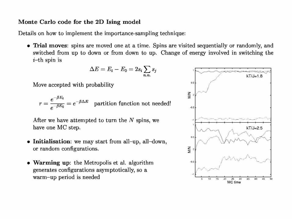
initial energy

MC steps: 1 step = 1 sweep over all spins

Here done in blocks of nblock steps

i,j: spin to be flipped

energy change

check for acceptance

a. Periodic boundary conditions

b. Minimum image convention

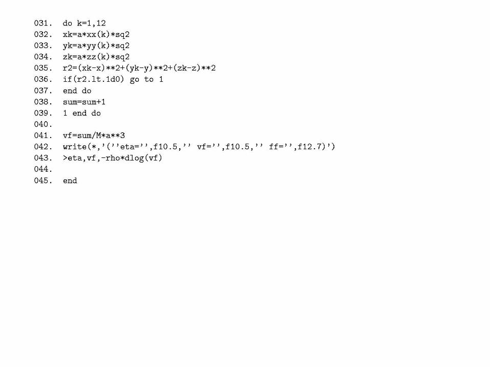
particles on sites of fcc lattice

periodic boundary conditions applied

histogram for g(r) accumulated

test position for k-th particle

check overlap with other particles

adjust acceptance ratio

to 50%

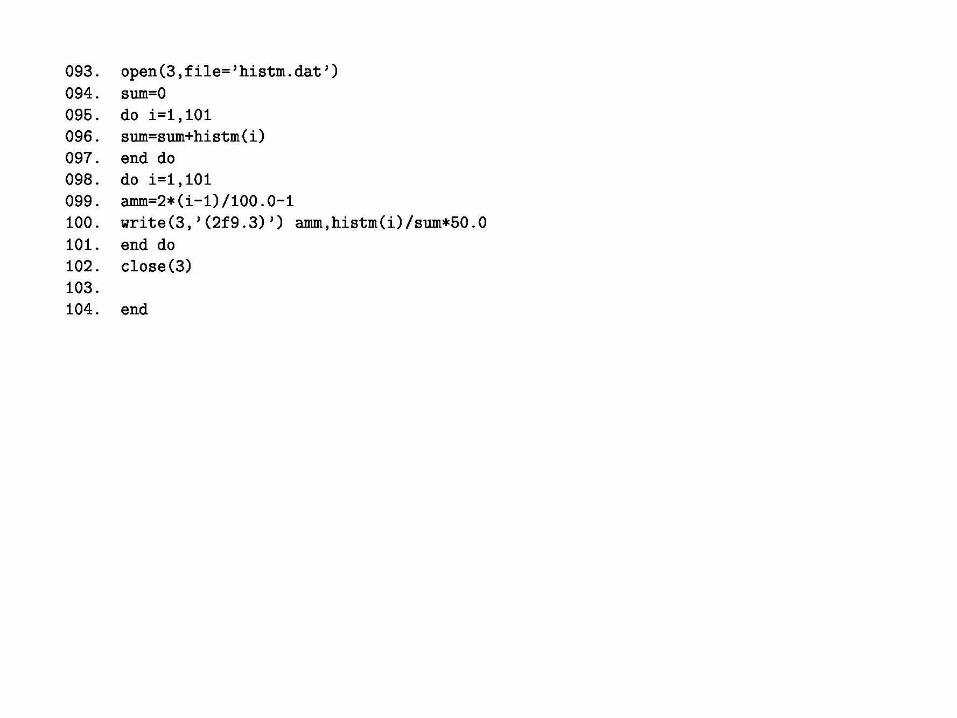
normalisation of g(r)

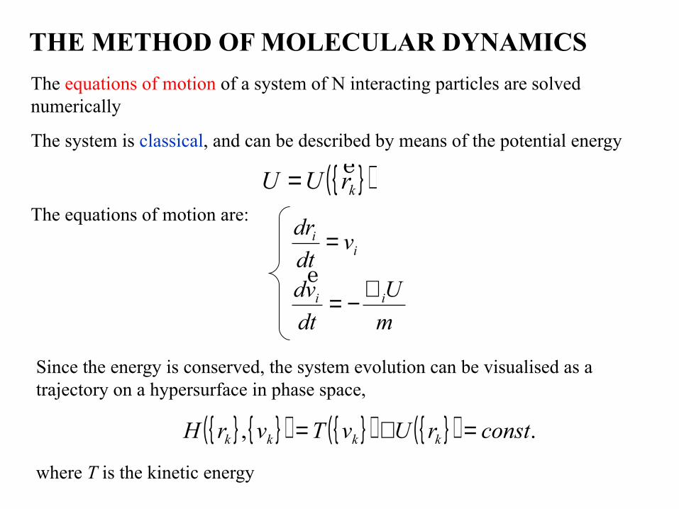
THE METHOD OF MOLECULAR DYNAMICS

The equations of motion of a system of N interacting particles are solved numerically

The system is classical, and can be described by means of the potential energy

{ }( )krUU=

The equations of motion are:

m

U

dt

vd

vdt

rd

ii

ii

∇−=

=

Since the energy is conserved, the system evolution can be visualised as a trajectory on a hypersurface in phase space,

where T is the kinetic energy

{ } { }( ) { }( ) { }( ) ., constrUvTvrH kkkk =+=

Integration methods

Based on finite difference schemes, in which time t is discretised using a time interval h

Knowing the coordinates and the forces at time t, the state at a later time t+h is obtained

The simplest (but still powerful!) algorithm is the Verlet algorithm

VERLET ALGORITHM

We write the following Taylor expansions:

++++=+ )(6

)(2

)()()(32

tvh

tFm

htvhtrhtr iiiii

+−+−=− )(6

)(2

)()()(32

tvh

tFm

htvhtrhtr iiiii

Adding, neglecting terms of order O(h4) , and rearranging:

The kinetic energy at time t can now be obtained as

)()()(2)(2

tFm

hhtrtrhtr iiii

+−−=+

This is a recurrence formula, allowing to obtain the coordinates at time t+h knowing the coordinates at times t and t-h

It is a formula of third order (the new positions contain errors of order h4)

The velocities can be obtained from the expansion:

)()(2)()( 2hOtvhhtrhtr iii ++−=+

as

h

htrhtrtv ii

i 2

)()()(

−−+=

(which contains errors of order h2)

∑=

=N

iic tvmtE

1

2)(

2

1)(

Using the equipartition theorem, the temperature can be obtained as

22

1 2 kTmv =α c

f

N

ii

f

EkN

vkN

mT

2

1

2 == ∑=

where

α = arbitrary degree of freedom

Nf = number of degrees of freedom

LEAP-FROG VERSION

Numerically more stable version than standard algorithm. We define:

h

trhtrhtv

h

htrtrhtv ii

iii

i

)()(

2 ,

)()(

2

−+=

+−−=

−

Positions are updated according to

++=+

2)()(

htvhtrhtr iii

)()()()()(2

tFm

hhtrtrtrhtr iiiii

+−−=−+

Using the Verlet algorithm,

so that

)(2

2

tFm

hhtv

htv iii

+

−=

+

Therefore leap-frog version or Hamiltonian version is

++=+

2)()(

htvhtrhtr iii

)(2

2

tFm

hhtv

htv iii

+

−=

+

222

)(

−+

+

=

htv

htv

tvii

i

The velocities are obtained as

Stability of trajectories

Systems with many degrees of freedom have a tendency to be unstable

If δ is the distance in phase space between two trajectories that initially are very close, and write

then the system is

tCet λδ =)(

• STABLE if δ < 0 or decreases faster than exponentially

• UNSTABLE if δ > 0; the system is said to be chaotic

λ = Lyapounov coefficient

Lyapounov instability is important because:

1. it limits the time beyond which an accurate trajectory can be found

2. to reach high accuracy after time t we need too many accurate decimal digits in the initial condition

ελ −= 100ce t

10log

log 0 tc λε −=

Since systems with many degrees of freedom are intrinsically unstable, very accurate integration algorithms are useless

The basic requirements that an algorithm should satisfy are:

1. Time reversibility:

Udt

vdm

vdt

rd

ii

ii

−∇=

=

The equations are invariant under the

transformations

tt −→

ii vv −→

The Verlet algorithm is time reversible

Irreversibility in some algorithms induces intrinsic energy dissipation so that energy is not conserved

)()()(2)(2

tFm

hhtrtrhtr iiii

+−−=+ )()()(2)(2

tFm

hhtrtrhtr iiii

++−=−hh −→

)()()(2)(2

tFm

hhtrtrhtr iiii

+−−=+

2. Symplecticity:

The probability distribution { } { }( )tvrf ii ,,

evolves like an incompressible

fluid, which implies 0=f

A symplectic algorithm conserves the volume of phase space

A molecular-dynamics FORTRAN code

• declare variables• starting positions and velocities

• initialise parameters

MD

loop

• update positions and velocities (leap frog)

loop

ove

r pa

irs o

f p

artic

les

• averages and print out

• calculate relative position (using minimum image convention)

• accumulate forces• accumulate energies, virial, etc.

• apply periodic boundary conditions

Maxwell-Boltzmann distribution for velocities

Particles initially on nodes of a fcc lattice

periodic boundary conditions

FORCE calculation

minimum image convention

add up forces to each member of ij pair

update velocities and positions

histogram for g(r)

normalise radial distribution function

FIN

FIN

/m

T({vk }) es la energía cinética

O(h2)