Finite element analysis of DNA supercoilingYang Yang, Irwin Tobias, and Wilma K. Olson Citation: The Journal of Chemical Physics 98, 1673 (1993); doi: 10.1063/1.464283 View online: http://dx.doi.org/10.1063/1.464283 View Table of Contents: http://scitation.aip.org/content/aip/journal/jcp/98/2?ver=pdfcov Published by the AIP Publishing Articles you may be interested in Polymer induced condensation of DNA supercoils J. Chem. Phys. 129, 185102 (2008); 10.1063/1.2998521 Structural optimization for heat detection of DNA thermosequencing platform using finite element analysis Biomicrofluidics 2, 024102 (2008); 10.1063/1.2901138 Influence of supercoiling on the disruption of dsDNA J. Chem. Phys. 123, 124901 (2005); 10.1063/1.2042367 Elastic theory of supercoiled DNA J. Chem. Phys. 83, 6017 (1985); 10.1063/1.449637 Estimating the torsional rigidity of DNA from supercoiling data J. Chem. Phys. 77, 580 (1982); 10.1063/1.443600

This article is copyrighted as indicated in the article. Reuse of AIP content is subject to the terms at: http://scitation.aip.org/termsconditions. Downloaded to IP:

137.189.170.231 On: Mon, 22 Dec 2014 02:25:09

Finite element analysis of DNA supercoiling Yang Yang, Irwin Tobias, and Wilma K. Olson Department of Chemistry, Rutgers, The State University of New Jersey, New Brunswick, New Jersey 08903

(Received 10 July 1992; accepted 29 July 1992)

A DNA polymer with hundreds or thousands of base pairs is modeled as a thin elastic rod. To find the equilibrium configurations and associated elastic energies as a function of linking number difference (aLk), a finite element scheme based on Kirchhoff's rod theory is newly formulated so as to be able to treat self-contact. The numerical results obtained here agree well with those already published, both analytical and numerical, but a much more detailed picture emerges of the several equilibrium states which can exist for a given aLk. Of particular interest is the discovery of interwound states having odd integral values of the writhing number and very small twist energy. The existence of a noncircular cross section, inhomogeneous elastic constants, intrinsic curvature, and sequence-dependent bending and twisting can all be readily incorporated into the new formalism.

LIST OF SYMBOLS The transformation matrix that relates the local coordinate system to the global coordinate system; given by Eq. (2.4).

AI' A2

c d\O)(S), d~O) (S), d~O)(S)

dieS), d2(s), d3(s)

e!, e2, e3

E, G, v

F

id

[K]

The area of a cross section of the unde­formed rod. The bending constants with respect to the two principal axes of a cross section of a rod. The twist constant. The local coordinate system defined on the cross section of the unstressed rod.

The local coordinate system defined on the cross section of the stressed rod. The fixed global Cartesian coordinate sys­tem. Young's modulus, the shear modulus, and Poisson's ratio, respectively. The resultant axial force on the deformed rod. The effective global load vector generated by intrinsic curvature, twist, and strain; defined by Eq. (3.19). The moments of bending and twisting in­ertia, respectively. The number of elements between the two contacted segments. Global stiffness matrix; defined by Eq. (3.18). Arclength between two contacted seg­ments. The global external load vector that de­pends on the applied concentrated force [pes ])] in Eq. (3.20). The vector that separates a pair of con­tact points. The position vector of a material point along the axis of the stressed rod. The arclengths that specify the beginning and ending points of the contact zone.

U(s) Wr, Tw, Lk

pes)

[(3]

Ie

II 0, ¢, ¢

A

[x]

J. Chern. Phys. 98 (2), 15 January 1993 0021-9606/93/021673-14$06.00

The transformation matrix that relates the curvature components and twist den­sity to Euler angles and their first deriv­atives; given by Eq. (2.7).

The axial displacement. The writhing number, the twist, and the linking number. The contact force distributed along the contact zone. The collective vector of contact forces at the contact nodal points; defined by Eq. (3.33).

The axial strain. The constraint for the position of one end of the rod. The constraint for the contact points. The vector containing the components of intrinsic curvature KIO), KiO) and twist density n (0) •

The vector containing the components of curvature KI> K2 and twist density n de­fined in the current stressed configura­tion. The potential energy. The Euler angles defined on the cross sec­tion of the deformed rod. The reactive force applied at the S = L end of the rod to keep it fixed at a specific position 'Y.

The ith nodal variable; 4 X 1 matrix con­taining the Euler angles and dimension­less axial displacement {O,¢,¢,U/a}, i=l, 2, ... , N+l. The global variable that is the collective vector of all the nodal variables X(i).

@ 1993 American Institute of Physics 1673 This article is copyrighted as indicated in the article. Reuse of AIP content is subject to the terms at: http://scitation.aip.org/termsconditions. Downloaded to IP:

137.189.170.231 On: Mon, 22 Dec 2014 02:25:09

1674 Yang, Tobias, and Olson: DNA supercoiling

I. INTRODUCTION

DNA usually occurs as a double helix with two com­plementary nucleotide chains winding around a common axis. In cells, the common axis of the DNA often folds into a supercoiled form that is linked to its biological func-t · 1-12 I h d h .. IOn. n ot er wor s, t e specIfic mterwound conforma-tion .of DNA facilitates various biochemical processes, in­cludmg replication, transcription, and recombination. Analysis of the topological and energetic aspects of super­coiled DNA is therefore essential for understanding both the initiation and the progress of these events.

The enormous size of supercoiled DNA currently pro­hibits conformational study at the atomic level. As a result, the double helical polymer is often modeled as a thin elas­tic isotropic rod with a circular cross section and no pref­erential directions of bending and twisting. Although this model greatly reduces the number of independent vari­ables, it still requires solving nonlinear differential equa­tions for which very limited mathematical tools are avail­able. Until now most solutions to the three-dimensional structure of supercoiled DNA have been obtained through intensive computer simulations, such as Monte Carlo cal­culations or energy minimization.9,13-16 While these studies have provided insightful views into the supercoiling of DNA, most of them are computationally time consuming and limited, so far, to the assumption that the elastic DNA is everywhere homogeneous and intrinsically straight. Thus, precluded from consideration are such interesting topics as base sequence effects and the influence of ligand binding on the conformations of supercoiled DNA.

In this paper we apply the finite element method com­monly used in engineering applications to examine the ev­olution of a DNA duplex, again modeled as an elastic rod from a relaxed to a highly supercoiled state. Now, how~ ever, the presence of inhomogeneities can naturally be in­corporated into the formalism so that the investigation of

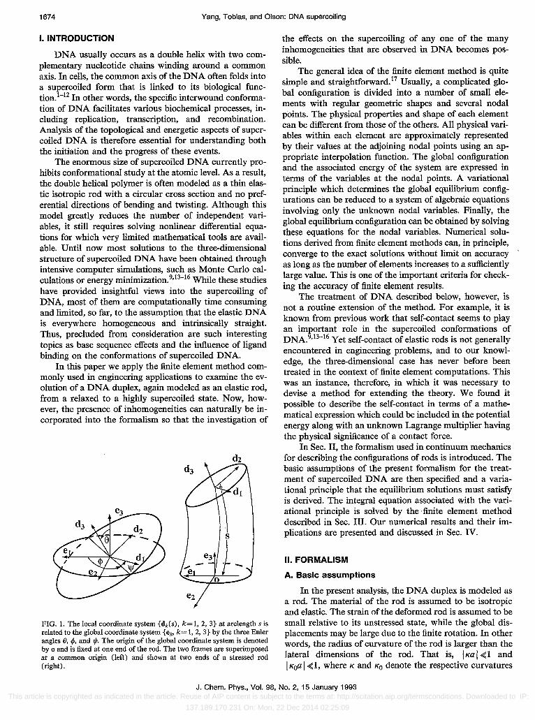
FIG. 1. The local coordinate system {dk(s), k= 1, 2, 3} at arclength s is related to the global coordinate system {e", k= 1,2, 3} by the three Euler angles e, <p, and ,p. The origin of the global coordinate system is denoted by 0 and is fixed at one end of the rod. The two frames are superimposed at a common origin (left) and shown at two ends of a stressed rod (right).

the effects on the supercoiling of anyone of the many inhomogeneities that are observed in DNA becomes pos­sible.

The general idea of the finite element method is quite simple and straightforward. 17 Usually, a complicated glo­bal configuration is divided into a number of small ele­ments with regular geometric shapes and several nodal points. The physical properties and shape of each element can be different from those of the others. All physical vari­ables within each element are approximately represented by their values at the adjoining nodal points using an ap­propriate interpolation function. The global configuration and the associated energy of the system are expressed in terms of the variables at the nodal points. A variational principle which determines the global equilibrium config­urations can be reduced to a system of algebraic equations involving only the unknown nodal variables. Finally, the global equilibrium configuration can be obtained by solving these equations for the nodal variables. Numerical solu­tions derived from finite element methods can, in principle, converge to the exact solutions without limit on accuracy as long as the number of elements increases to a sufficiently large value. This is one of the important criteria for check­ing the accuracy of finite element results.

The treatment of DNA described below, however, is not a routine extension of the method. For example, it is known from previous work that self-contact seems to play an important role in the supercoiled conformations of DNA.9,13-16 Yet self-contact of elastic rods is not generally encountered in engineering problems, and to our knowl­edge, the three-dimensional case has never before been treated in the context of finite element computations. This was an instance, therefore, in which it was necessary to devise a method for extending the theory. We found it possible to describe the self-contact in terms of a mathe­matical expression which could be included in the potential energy along with an unknown Lagrange multiplier having the physical significance of a contact force.

In Sec. II, the formalism used in continuum mechanics for describing the configurations of rods is introduced. The basic assumptions of the present formalism for the treat­ment of supercoiled DNA are then specified and a varia­tional principle that the equilibrium solutions must satisfy is derived. The integral equation associated with the vari­ational principle is solved by the' finite element method described in Sec. III. Our numerical results and their im­plications are presented and discussed in Sec. IV.

II. FORMALISM

A. Basic assumptions

In the present analysis, the DNA duplex is modeled as a rod. The material of the rod is assumed to be isotropic and elastic. The strain of the deformed rod is assumed to be smail relative to its unstressed state, while the global dis­placements may be large due to the finite rotation. In other words, the radius of curvature of the rod is larger than the lateral dimensions of the rod. That is, I Ka I ~ 1 and IKoal ~1, where K and KO denote the respective curvatures

J. Chern. Phys., Vol. 98, No.2, 15 January 1993 This article is copyrighted as indicated in the article. Reuse of AIP content is subject to the terms at: http://scitation.aip.org/termsconditions. Downloaded to IP:

137.189.170.231 On: Mon, 22 Dec 2014 02:25:09

Yang, Tobias, and Olson: DNA supercoiling 1675

in the currently stressed and the initially unstressed states, and a is the maximum radius of the undeformed cross sections. Based on these fundamental assumptions, the first-order theory of elastic rods, Kirchhoff's theory of rods, can be derived within the framework of continuum mechanics. 18 This theory is employed in the present paper to derive a variational principle for the finite element anal­ysis of DNA.

B. Description of configurations

For convenience, we choose the unstressed rod as the reference configuration. In this configuration, the axis of the rod can be represented by a space curve with position vector Ro(S) in a fixed Cartesian coordinate system {el' e2' e3} where the parameter S denotes the arclength measured from one end of the rod. Two orthogonal unit vectors din) (S) and d~O) (S) are chosen to lie along the principal axes of a cross section of the rod. The position vector of a material point in the cross section is then given by

2

R(X!> X 2, S)=Ro(S)+ I xjdfO)(s), (2.1) i=1

where XI and X 2, the material coordinates in the orthog­onal basis {d\O) (S), d~O)(S)}, are used to specify the posi­tion of a material point in a cross section at arclength S.18,19

The unit tangent vector to the axis is given by

dRo(S) toeS) dS (2.2)

We introduce another unit vector diO) (S) that coin­cides with the tangent toeS) so that {d\O)(S), diO) (S), d~O) (S)} can be arranged to form a local right-handed orthogonal basis. Once the orientation of this basis is de­termined, the position of every material point in the rod is given by Eq. (2.1).

The orientation of the local coordinate systems {dIO) (S), d~O) (S), din) (S)} is determined here by the Euler angles {eo, tPo, tPo} (see, for example, Fig. 1). As a result, the local coordinate system {din) (S), din) (S), din) (S)} can be related to the fixed Cartesian coordinate frame {el' e2' e3} by the transformation

(2.3)

where

cos tPo cos tPo - cos eo sin tPo sin tPo sin tPo cos tPo+coseo.cos tPo sin tPo sin eo sin tPo 1 sin eo cos tPo . [TI (S)] = -cos tPo sin tPo-cos eo sin tPo cos tPo -sin tPo sin tPo+cos eo cos tPo cos tPo (2.4)

sin eo sin tPo

Once the Euler angles eo, tPo, and tPo are given along the unstressed axis, the rate of change of {d~O) (S), i= 1,2,3} with respect to arclength S can be written as

dd~O) (S) (0) (0) dS K Xdj (S). (2.5)

The vector K(O) is the angular rate of rotation of the local coordinate frame {d}O) (S), i= 1,2,3} with respect to movement along the rod. Written out in terms of its com­ponents,

K(O) =KiO)diO) (S) +KiO)diO) (S) +n(O)d~O) (S),

where K\O), KiO) are the components of intrinsic curvature, and n (0) is the intrinsic twist density of the rod. 18,19

Substitution of Eq. (2.3) into Eq. (2.5) yields the ex-pression for K(O) in the form

K(O) 1 eo Kio) = [T2 (S)] tPo , nCO) tPo

(2.6)

where

- sin eo cos tPo

cos tPo

[T2(S)j= -sintPo

o

cos eo

sin eo sin tPo 0 1 sin eo cos tPo 0,

cos eo I

(2.7)

and the prime symbol denotes the derivative of a variable with respect to the arclength of the unstressed rod.

Now let us consider the description of the rod in the stressed state. The position vector of the axis is

fO=fO(S), (2.8)

where the parameter s is the arclength of the stressed axis. The arclength of the deformed rod can be related, in turn, to the arclength of the unstressed axis S through

s(S) =S + U(S), (2.9)

where U(S) is the axial displacement defined along the axis of the unstressed rod. We can also associate with each value of s on the stressed rod the same axial displacement U(s) for each material point. This leads to the relationship

S(s) =s- UC'S) ,

where, U(S) = U(s).

J. Chern. Phys., Vol. 98, No.2, 15 January 1993 This article is copyrighted as indicated in the article. Reuse of AIP content is subject to the terms at: http://scitation.aip.org/termsconditions. Downloaded to IP:

137.189.170.231 On: Mon, 22 Dec 2014 02:25:09

1676 Yang, Tobias, and Olson: DNA supercoiling

The tangent unit vector t(s) of the stressed axis is given by

dro dS= [1 +E(S) ]t(s), (2.10)

where E(S) is the axial strain with respect to the reference configuration and is defined as

dUeS) E(S) =---as' We may also define the axial strain with respect to the

current (stressed) configuration as

dUes) E(S)=-a;-. (2.11)

It can be shown that E(S) equals E(S) up to the first order. In the current configuration, let {dk(s), k= 1,2,3} de­

note the three axes deformed from the corresponding axes {dJO) (S), i = 1,2,3} in the unstressed reference configura­tion (Fig. O. It can be shown within the first-order ap­proximation that {dk(s), k= 1,2,3} still forms an ortho­normal triad and that d3(s) coincides with the tangent unit vector t(s).18 Thus,

(2.12)

where

IC=Kldl (s) +K2d2(S) +Od3(s),

and KI, K2 are the components of curvature and 0 the twist density of the stressed rod. Note that the angular rate of rotation IC(S) is now defined along the axis of the stressed rod.

The orthogonal unit vectors {dk(s), k= 1,2,3} of the stressed rod can be related to the fixed Cartesian coordi­nate frame {e", k= 1,2,3} through a relationship analo­gous to Eq. (2.3),

[ ::~:~] =[TI(s)] [::]. d3(s) e3

(2.13)

Here the matrix [TI(S)] is of the same form as [TI(S)] in Eq. (2.4) with 0o, <Po, and t/Jo replaced by 0, <P, and t/J. Thus, the tangent unit vector t(s) in Eq. (2.10) is also given by d3 (s) in Eq. (2.13).

Similarly, IC can be expressed in terms of the Euler angles withEq. (2.13) substituted into Eq. (2.12). This gives

[ ::~:~] = [T2 (s)] [::], O(s) t/J'

(2.14)

where [T2(s)] is defined analogously to [T2(S)] in Eq. (2.7) with 0o, <Po, and t/Jo replaced by 0, <p, and t/J, and the prime symbol is used to denote the derivative of a variable with respect to the arclength of the stressed rod.

From the above, it is seen that the three Euler angles {O(s), <p(s), t/J(s)} and the axial displacement U(s) are the

minimum set of independent variables needed to describe configurations of a stressed rod. Once the values of the Euler angles and of U(s) are given along the axis of a stressed rod, the curvature, the twist, and the axial strain of the rod can be evaluated by Eqs. (2.14) and (2.11). The variables {O(s), <p(s), t/J(s), U(s)} associated with an equi­librium state are determined by considering the global equilibrium conditions discussed in the following sections.

c. Variational principle

The variational principle, which gives the global equi­librium configurations of a stressed rod, can be expressed as follows: Among all kinematically admissible solutions which satisfy the boundary conditions on an elastic rod, the actual solution to the eqUilibrium equations makes the first variation of the constrained potential energy 11* van­ish. That is,

SII*=SII -sr I-sr 2 =0, (2.15)

where II is the potential energy, r I the position constraint on the end of the rod, r 2 the constraint on the contact zone, and 1I*=II-rl-r2.

The potential energy II of the rod can be expressed as

(2.16)

where Wei and W ext denote the elastic energy and the work done by external loads, respectively, and can be written as

rL [Ell (0) 2 EI2 (0) 2 We\= Jo 2 (KI-KI ) +2 (K2-K2 )

GJ Ed ] +2 (0-0(0»2+2 ~ ds, (2.17)

L n

W ext= fo [f· (ro-Ro) +m' 0]ds+ j~1 {M(sj) ·0(sj)

+ P(Sj) • [ro(sj) - Ro(Sj) ]}. (2.18)

The center dot in the above expression denotes the scalar product of two vectors and L is the length of the stressed rod. The vectors f and m are, respectively, the resultant force and resultant moment of the distributed surface and body forces per unit arclength of the stressed rod, and M(sj) and P(Sj) are, respectively, the concentrated mo­ments and forces applied at arclength S=Sj along the stressed rod. The parameters Sj and Sj refer to the arclengths associated with the same material point in the unstressed and stressed states. The angular displacement 0 is defined as

0(s)= f: (IC-IC(O»ds.

The parameter E is Young's modulus and G is the shear modulus.2o Their ratio is determined by Poisson's ratio v through E/G=2(1 +v). The symbol d is the area of the cross section in the reference configuration. The parame­ters I I and h are the moments of inertia with respect to the axes dlO) (S) and d~O) (S) and are given by

J. Chern. Phys., Vol. 98, No.2, 15 January 1993 This article is copyrighted as indicated in the article. Reuse of AIP content is subject to the terms at: http://scitation.aip.org/termsconditions. Downloaded to IP:

137.189.170.231 On: Mon, 22 Dec 2014 02:25:09

Yang, Tobias, and Olson: DNA supercoiling 1677

11= f.<J!'X~dd, 12= f.<J!'X~dd. The elastic bending constants are normally defined as

AI =E II and A2=E 12, while the twist constant is written as C= GJ, where

f ( 2 2 a<l> a<l> ) J= .If Xl+Xi+XlaX2-X2aXl dd.

<I> is the warping function of the cross section that de­scribes the out-of-plane distortion of the transverse cross sections of the rod and can be shown to be zero for circular cross sections. 20

The first variations of the elastic energy and the work then follow as

8Wel= SoL [EII(KI-K\0»8Kl+Eh(K2-KiO»8K2

+GJ(n-n(0»8n+Eds8e]ds, (2.19)

(2.20)

The constraint function r 1 in Eq. (2.15) can be writ­ten as

(2.21 )

where the vector A is the Lagrange multiplier, correspond­ing to the unknown reactive force which must be applied at

Solving Eq. (2.25) will yield the global equilibrium con­figurations of the stressed rod. Note that without comput­ing the second variation of the constrained potential energy we cannot distinguish the stable equilibrium states from the unstable ones. Equation (2.25) as it now stands cannot be solved analytically. For this reason we employ a finite element method, described in the next section, to obtain a numerical solution.

It is worth mentioning that our treatment of self­contact is similar in certain respects to that developed by Bottega in his study of the delamination problem.21 Al­though the mechanism of his two-dimensional contact problem is very different from that in the present three­dimensional self-contact problem, his method may be use-

the end of the rod (s= L) in order to keep the end fixed at a given position y. For a closed rod, y=ro(O).

The last term r 2 in the constrained potential energy ll* is introduced in order to treat self-contact. It has the form

(2.22)

where Sa and sb are the arclengths at the beginning and the end of one contact segment and Ld is the arclength that separates two contacted segments. A point at s, where sa<;,s<;,sb, makes direct contact with the point at L d+2sb-s. In Eq. (2.22) (J(s) is another Lagrange mul­tiplier having the significance of being an unknown contact force distributed along the rod within the contact zone. Since a rod has finite thickness, a pair of contact points on the axis of a rod is actually separated by a finite distance and orientation which is represented by the vector valued function ris). For a self-contacted rod with uniform cir­cular cross section of radius a, rd(s) may be written as

rd(s) =2aV(s)

with the unit vector V (s) defined by

V d3(Ld+2sb-s) Xd3 (s)

Id3(Ld+2sb~S) Xd3 (s) I .

(2.23)

(2.24)

When we combine Eqs. (2.19)-(2.23), the variational principle, Eq. (2.15), can be rewritten in the form

(2.25)

ful in the analytical study of three-dimensional contact problems.

III. FINITE ELEMENT ANALYSIS

A. Basic formulas

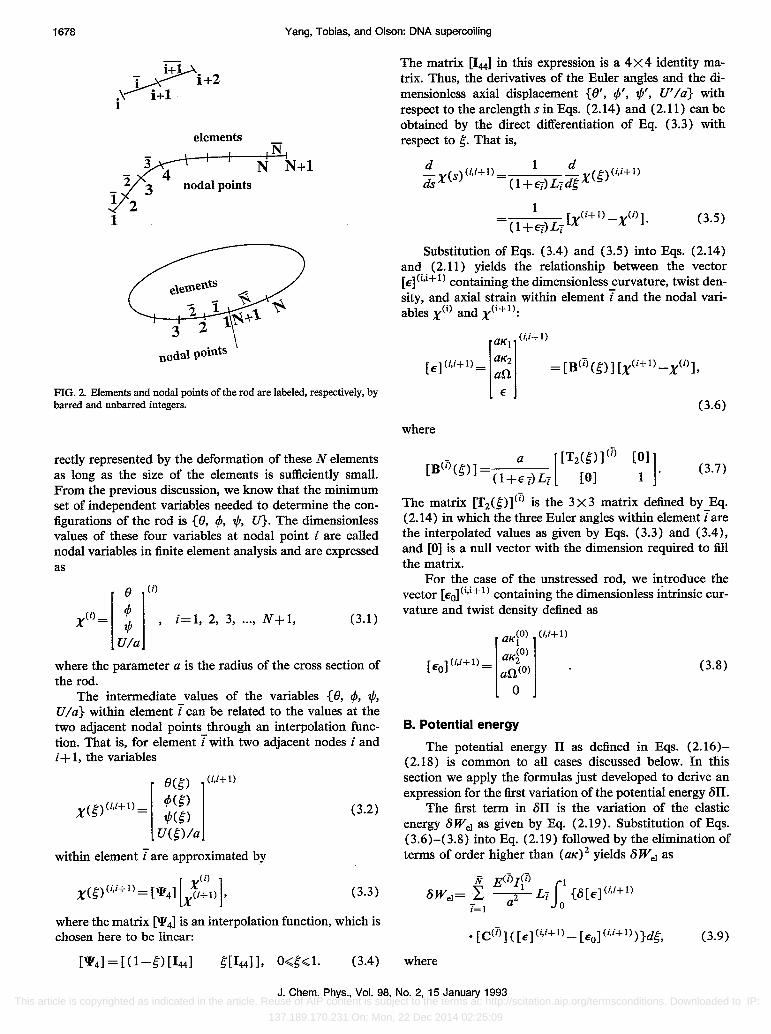
In a finite element analysis, a rod is first divided into a sequence of N elements and N + 1 nodal points. Both the elements and the nodal points are labeled by a series of consecutive integers, denoted by {l,i,3, ... ,.&} and {1,2,3, ... ,N + I}, respectively, as shown in Fig. 2. Each element has initial length Ly, cross-section area dy, and elastic constants E(i) and veT). These geomet­ric and physical properties can differ from one element to the next. Normally, configurations of the rod can be cor-

J. Chern. Phys., Vol. 98, No.2, 15 January 1993 This article is copyrighted as indicated in the article. Reuse of AIP content is subject to the terms at: http://scitation.aip.org/termsconditions. Downloaded to IP:

137.189.170.231 On: Mon, 22 Dec 2014 02:25:09

1678 Yang, Tobias, and Olson: DNA supercoiling

~ .~ ~ i+2 .\ i+l I

elements

N N+l nodal points

3 nodal points

FIG. 2. Elements and nodal points of the rod are labeled, respectively, by barred and unbarred integers.

reetly represented by the deformation of these N elements as long as the size of the elements is sufficiently small. From the previous discussion, we know that the minimum set of independent variables needed to determine the con­figurations of the rod is {O, cp, 1/1, U}. The dimensionless values of these four variables at nodal point i are called nodal variables in finite element analysis and are expressed as

o cp 1/1

Ula

(i)

, i=l, 2, 3, ... , N+1, (3.1)

where the parameter a is the radius of the cross section of the rod.

The intermediate values of the variables {O, cp, 1/1, Ula} within element T can be related to the values at the two adjacent nodal points through an interpolation func­tion. That is, for element T with two adjacent nodes i and i+ 1, the variables

O(S') W+ 1)

cp(S')

1/1(S') (3.2)

U(S')la

within element T are approximated by

(3.3 )

where the matrix ['1'4] is an interpolation function, which is chosen here to be linear:

(3.4)

The matrix [144] in this expression is a 4 X 4 identity ma­trix. Thus, the derivatives of the Euler angles and the di­mensionless axial displacement {O', cp', 1/1', U'la} with respect to the arclength s in Eqs. (2.14) and (2.11) can be obtained by the direct differentiation of Eq. (3.3) with respect to S'. That is,

1 d (i,i+ 1)

(1 +€f-)LjdS'X(S')

1 [X(i+l)-X(i)]. (3.5) (1+ey)Lj

Substitution of Eqs. (3.4) and (3.5) into Eqs. (2.14) and (2.11) yields the relationship between the vector [E](i,i+1) containing the dimensionless curvature, twist den­sity, and axial strain within element T and the nodal vari­ables XCi) and X(i+l):

aKI W+l)

[E]W+1)= :~ = [B(i)(S')][X(i+1)-X(i)],

€

(3.6)

where

a [[T2(S')] (i)

(1 +q) L[ [0] (3.7)

The matrix [T2(S')]cil is the 3X3 matrix defined by Eq. (2.14) in which the three Euler angles within element Tare the interpolated values as given by Eqs. (3.3) and (3.4), and [0] is a null vector with the dimension required to fill the matrix.

For the case of the unstressed rod, we introduce the vector [EO] (i,i+1) containing the dimensionless intrinsic cur­vature and twist density defined as

[EO] W+ 1) =

aK(O) 1

aK(O) 2

aU(O)

o

B. Potential energy

W+ 1)

(3.8)

The potential energy II as defined in Eqs. (2.16)­(2.18) is common to all cases discussed below. In this section we apply the formulas just developed to derive an expression for the first variation of the potential energy «SII.

The first term in «SII is the variation of the elastic energy «SWel as given by Eq. (2.19). Substitution of Eqs. (3.6)-(3.8) into Eq. (2.19) followed by the elimination of terms of order higher than (aK)2 yields «SWel as

N Ecil1cil 1

«SWeI=L o~Lj r {«S[E]W+ 1)

[=1 a Jo

(3.9)

where

J. Chern. Phys., Vol. 98, No.2, 15 January 1993 This article is copyrighted as indicated in the article. Reuse of AIP content is subject to the terms at: http://scitation.aip.org/termsconditions. Downloaded to IP:

137.189.170.231 On: Mon, 22 Dec 2014 02:25:09

Yang, Tobias, and Olson: DNA supercoiling 1679

1 0 0 0

l(l)

0 2

0 0 IV)

[CO)] = O<Y),jY) 0 0 Em 1m 0

1

(3.10)

.s;ICY)a2

0 0 0 l(i)

I

Here the superscript (T) denotes the parameters associated with element T. If the elastic constants and geometric pa­raIl!eters are given as functions of the arclength s, then [CU)] can vary within element T. Note that [e](i,i+l) de­pends on the nodal variables XCi) and XU+ I) at two adja­cent points i and i+ I through Eq. (3.6). Therefore 8 Wei is determined by all the nodal variables {XCi), ;=1, 2, 3, ... , N+l}.

The second term in 8IT is the variation of the external work, 8Wcxt> as given by Eq. (2.20). We consider the case where the only contribution to Wext comes from a single concentrated force peS]) applied at the point in element] having arclength S]. The first variation of the work can then be expressed as

8W cxt=&o(S]) • P(S]),

and the arclength S] can be written as j-I S]= L (1+ey)Ly+L]5],·

7=1

(3.11)

If we fix one end of the rod at the origin of the Carte­sian coordinate system {el> e2, e3}, then the variation &o(S]) is given by

&o(S]) =8 J: d3(s)ds, (3.12)

where d3(s) is given by Eq. (2 .. )3). The substitution ofEq. (3.3) into Eq. (2.13) gives d~i), which when introduced in Eq. (3.12), yields the expression for l)ro(s]),

j-I il ..,.. [l)xCi) 1 &o(S]) = _L Ly [TNCI)]d5 l)CHI)

;=1 0 X

(3.13)

where [TN(i)] is a 3 X 8 matrix given in detail in Eq. (Al) in the Appendix. Substitution of this equation into Eq. (3.11) reduces the variation of the external work to

+L] J:7 [TNO)]d~[ l)!fj~)1) l}' [P(S])].

(3.14)

By introducing a global nodal variable [x] which is the collective vector of the nodal variables XCi), i = 1, 2, 3, ... , N + 1, we obtain

XCI)

[x]= X (2 )

(3.15)

XCN+I)

and then following the standard procedures of the finite element method,!7 we can rewrite Eqs. (3.9) and (3.14) in global form as

l)We1=l)[x]' [K] [X] -S[X]· [Feld,

l)Wext=l)[X]' [Pg ],

(3.16)

(3.17)

where [K] is a supermatrlx of order 4(N + 1) X 4(N + 1) called the global stiffness matrix. Details of its assembly from the identity

-l)XU)]

• [c(i)] [B(i)] [XU+1) -xU)]dg (3.18)

are found in Ref. 17. Here we have introduced the nodal variables as given by Eq. (3.6) into Eq. (3.9).

Similarly, the vector [Feff] in Eq. (3.16) denotes the effective global load vector generated by the initial curva­ture and twist density, and can be deduced from

N E(i)1 (7) il -l)[X]'[Feff]= _L a 21 Ly [BU)][l)XU+!)-l)X(i)]

;=1 0

(3.19)

The vector [Pg] in Eq. (3.17) is called the global ex­ternal load vector and is defined by

S[x]· [Pg ] = [TN(s]) ]S[X] • [P(S])], (3.20)

where [T N(S] )] is another supermatrix of order 3 X 4(N + 1) and is derived from the identity

(3.21 )

Subtracting Eq. (3.17) from Eq. (3.16), we get the variation of the potential energy l)IT in global form as

l)IT=l)[x]' ([K] [X] - [Feff] - [Pg ]). (3.22)

In the following three subsections, we discuss the global expression of the variational principle (2.25) for three fun­damental cases.

J. Chern. Phys., Vol. 98, No.2, 15 January 1993 This article is copyrighted as indicated in the article. Reuse of AIP content is subject to the terms at: http://scitation.aip.org/termsconditions. Downloaded to IP:

137.189.170.231 On: Mon, 22 Dec 2014 02:25:09

1680 Yang, Tobias, and Olson: DNA supercoiling

C. An open rod of finite length without self-contact

Consider an open rod of finite length, which could be initially straight or curved, subject to a point force some­where along its axis, but without any contact. between dis­tant material points on the rod during the deformation. In this case, the constrained potential energy IT* equals the potential energy IT and the equilibrium configurations are determined by

SIT*=SIT=O,

where SIT is given by Eq. (3.22). Since the components of the variation S[x] in Eq.

(3.22) are arbitrary and independent, the above equation can be further simplified to the following system of alge­braic equations:

(3.23)

Solution of Eq. (3.23) yields the equilibrium configu­rations of the rod. Since both [K] and [Felf] implicitly de­pend on the unknown current configuration [x], Eq. (3.23) has to be solved iteratively. A simple iteration procedure is adopted here and its general scheme is summarized below.

The concentrated force P (s j) is gradually increased from zero to its specified value in increments of (l!m)P(sj). The initial configuration [x](o) is used as the trial solution for the first incremental state with load (l!m)P(sj). After evaluation of [K] and [Felf] by Eqs. (3.18) and (3.19), the solution [x](1) is obtained using the following expression:

(3.24)

where n = 1 corresponds to the first increment of P (s j ). The SUbscripts 7"-1 and 7" refer to two successive steps in the iterative scheme used to obtain a solution when the load is (n/m)[P(s j)]. This simple iteration is repeated until the solution converges, that is, until 1[x](1") - [x](1"-i) 1 < e, the desired numerical accuracy. For the nth incremental state at load (n/m)P(sj), the solution to the (n - 1) th state is used as the initial trial solution. [K](n-i) and [Felf](n-1) are calculated, respec­tively, from Eqs. (3.18) and (3.19), and [x] is obtained iteratively from Eq. (3.24). Repetition of these steps until n=m will yield the current eqUilibrium configuration un-der the applied load P(Sj). '

D. A spatially constrained rod without self-contact

Let us consider the deformation of a spatially con­strained rod without self-contact. One end of the rod, S ='0, is fixed at the origin of the global coordinate system {ei' e2, e3} and the other end, S=L, is subject to the constraint r i and is fixed at the position 'Y. In this case r i

should be included in the variational principle which takes the form

(3.25)

We take the first variation of r i in Eq. (2.21) and use Eq. (3.21) with Sj= L to obtain

sri = [TN(L) ]S[X] • [A] +8[A]· [ro(L) -'Y], (3.26)

where [TN(L)] is defined by Eq. (3.21). For the case ofa closed rod, 'Y=ro(O) =0. Note that ro(L) depends on the unit tangent vector t in the form of an integral over the entire length of the rod, and that t, which is identical to d3,

is related to the nodal variables {XCi), i= 1, 2, 3, ... , N + I} by Eqs. (2.13) and (3.3). Obviously, ro(L) cannot be ex­plicitly written in terms of [x]. However, when the current configuration [x](1") is sufficiently close to the previous one, [x](1"-I)' ro(L) can be expanded in the form

4(N+i) aro(L) ro(L)(1")=ro(L)(1"-1)+ L Jv

J. (Xj(1")-Xj(1"~1)

j=i .A.

+O( 1 [xi(1") - [X] (1"-1) 12),

where Xj is the component of vector [x] and the third term is a small quantity with order higher than 1 [x] (1") -[x](1"-i) I·

The second term in the above expression is analogous to &o(L) as given by Eq. (3.21) with S[x] replaced by X(1")-X(1"-1). This substitution leads to the following ex­pression correct to the first order:

ro(L) (1") =ro(L) (1"-1)

+ [TN(L)] (1"-I){[X] (1")- [X] (1"-il}'

Using the above equation, we can express the first vari­ation of r i as

sr l =[TN(L)](1"_I)S[X]' [A](1")+S[A]

• {ro(L) (1"-1) - [TN(L)] (1"-1) [X] (1"~1) -'Y}

(3.27)

Through combination of Eqs. (3.22) and (3.27), the variational principal can be expressed as

S[X] • {[K] (1"-1) [X] (1") - [Felf] (1"-1) - [Pg ]}

-[TN(L)](1"-1)S[X]' [A] (1")

-S[A]· [TN(L)] (1"-1) [X] (1")-S[A]

• {ro(L) (1"-1) - [TN(L)] (1"-1) - [X] (1"-i) -'Y}=O. (3.28)

Note that [x] and [A] are independent variables and their first variations S[x] and S[A] can be arbitrary. Thus, by using the identity ,

. [TN(L)] (1"-1)S[X] • [A]=S[X]' [TN(L)]f,._I)[A],

where the superscript T denotes the transpose, we can re­duce Eq. (3.28) to a system of algebraic equations for [x](1") and [A](1")'

[

[K](1"_I)

- [TN(L)] (1"-1)

J. Chern. Phys., Vol. 98, No.2, 15 January 1993 This article is copyrighted as indicated in the article. Reuse of AIP content is subject to the terms at: http://scitation.aip.org/termsconditions. Downloaded to IP:

137.189.170.231 On: Mon, 22 Dec 2014 02:25:09

Yang, Tobias, and Olson: DNA supercoiling 1681

Here [0] is a null matrix of the dimension required to fill the matrix on the right-hand side of the expression. Equa­tion (3.29) is solved iteratively by the use of a scheme analogous to that presented in Sec. III C. In this case, instead of gradually changing the load pes 7)' we vary the constrained position vector r incrementally until it reaches the origin to form a closed rod.

E. A closed rod with self-contact

To consider self-contact between distant parts of a closed rod, the term r 2 must be included in the variational principle. Let us first consider the expression for r 2 in terms of the global nodal variable IX] and the contact force {3.

Suppose there is one contact zone Sa <S <Sb

which con~in~ pairs of contact elements labeled by {ie, ie+l, ... , ie+n-l} and {ie+2n+id-l, ie+2n+id-2, ... , ie+n+id}, where id is the number of elements between the two contact points at S=Sb and S=Sb

+ L d• The contact force (3 can be represented by a series of contact point forces at the contact nodal points. The inter­mediate contact force within contact element T can be ex­pressed in terms of the contact forces at the two adjacent nodal points i, i + 1 through a linear interpolation function. Thd~ .

(3.30)

where

(3.31)

and [133] is the 3 X 3 identity matrix. Substituting Eq. (3.30) into Eq. (2.22) and taking its

first variation, we get the finite element expression for lir 2:

- [TN(L)] [,.-1) [0]

[0]

- [UK] [,.-1)

[0]

[0]

We consider the case where [Pg] equals zero. We ob­tain a number of successive eqUilibrium solutions to Eq. (3.35) by rotating one end of the closed rod at S = L with respect to the other end at S=O. At each fixed rotation, we vary the number of elements within the contact zone until the elastic energy reaches a minimum and the contact forces become repulsive. The matrix on the left-hand side of Eq. (3.35) and the vector on the right-hand side of Eq. (3.35) are calculated from the configuration IXkr-l)

(3.32)

The variations of ro(Ld +2sb -s) and roes) can be re­lated to the global nodal variable IX] by Eq. (3.21). How­ever, fo(Ld+2sb-s) and foeS) can only be related to IX] in a recursive form analogous to Eq. (3.28). The detailed derivation is algebraically tedious and thus omitted here.

Let [(3] be the collective vector of contact forces at the nodal points within the contact zone:

[PI ~ [p(~l:~l) 1 (3.33 )

Equation (3.32) may then be rewritten in global form as

I5r2 =15[{3]' [UK] (1'-1) [X] (1')+15[{3] • [q](1')

-c5[{3]. [UK] (1'-1) [X] (1'-l)-c5[{3] • [Rd] (1'-1)

(3.34)

where [q], [Rd] , and [Vii are given, respectively, by Eqs. (A2), (A3), and (AS) in the Appendix.

By combining Eqs. (3.29) and (3.34), we obtain the global expression of the variational principle for a rod with self-contact. It can then be reduced to a system of algebraic equations involving the unknown independent variables 1X](1')' [A](1')' and [(3](1') in the following form:

[X] (1') [A](1') [(3] (1')

[Pelf] (1'-1) + [P g] fo(L)(1'-l)-[TN (L)](1'-l)[X](1'-l)-r . (3.35)

[q] - [UK] (1'-1) [X] (1'-1) - [Rd] (1'-1)

which is obtained in the 'previous step of the iteration. The iterative procedure followed here is analogous to that pre­sented in Sec. III C.

IV. NUMERICAL RESULTS AND DISCUSSION

A. Open rod without self-contact: Convergence of numerical calculations

Before performing numerical calculations on closed DNA models, we vary the number of elements and check

J. Chem.,Phys., Vol. 98, No.2, 15 January 1993 This article is copyrighted as indicated in the article. Reuse of AIP content is subject to the terms at: http://scitation.aip.org/termsconditions. Downloaded to IP:

137.189.170.231 On: Mon, 22 Dec 2014 02:25:09

1682 Yang, Tobias, and Olson: DNA supercoiling

w

(b)

10,--------------.

o+-~.-~~-~~-~~-~~ 0.0 0.2 0.4 0.6 0.8

WIL

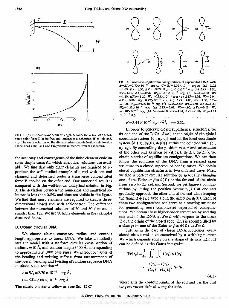
FIG. 3. (a) The cantilever beam of length L under the action of a trans­verse point force P at its free end undergoes a deflection Wat this end. (b) The exact solution of the dimensionless load-deflection relationship (solid line) (Ref. 31) and the present numerical results (squares).

the accuracy and convergence of the finite element code on some simple cases for which analytical solutions are avail­able. We find that only eight elements are required to re­produce the well-studied example of a rod with one end clamped and deformed under a transverse concentrated force P applied on the other end. Our numerical result is compared with the well-known analytical solution in Fig. 3. The deviation between the numerical and analytical so­lutions is less than 0.5% and thus not visible in the figure. We find that more elements are required to treat a three­dimensional closed rod with self-contact. The difference between the numerical solutions of 60 and 80 elements is smaller than 1 %. We use 80 finite elements in the examples discussed below.

B. Closed circular DNA

We choose elastic constants, radius, and contour length appropriate to linear DNA. We take an initially straight model with a uniform circular cross section of radius a= 10 A, and contour length 3400 A, corresponding to approximately 1000 base pairs. We introduce values of the bending and twisting stiffness from measurements of the overall bending and twisting of random sequence DNA in dilute NaCI solution:22

A = Ell =2.70X 10-11 erg A, C=GJ=2.04x 10-11 erg A.

The elastic constants follow as (see Sec. II C)

90=-~:r ?T ?T ,., 6 -"'" '" tl W!/ ,., 6 r FIG. 4. Successive equilibrium configurations of supercoiled DNA with A=EI[=2.70XIO- 11 erg A, C=GJ=2.04XIO- 11 erg A; (a) !J.Lk = 1.00, Wr= 1.00, !J.Tw=O.oo, We[=0.45 X 10-[2 erg; (b) !J.Lk= 1.98, Wr= 1.00, !J.Tw=0.98, We[=0.56x 10-[2 erg; (c) !J.Lk=3.oo, Wr = 1.80, !J.Tw= 1.20, We[=O.92 X 10- [2 erg; (d) !J.Lk=3.02, Wr=2.94, !J.Tw=0.08, We[=0.79 X 10-[2 erg; (e) !J.Lk=4.oo, Wr=3.oo, !J.Tw =1.00, We[=0.92XIO-[2 erg; (f) !J.Lk=5.oo, Wr=3.80, !J.Tw=1.20, We[=1.28XIO-[2 erg; (g) !J.Lk=5.03, Wr=4.90, !J.Tw=0.13, Wei = 1. lOX 10- 12 erg; (h) !J.Lk=6.oo, Wr=4.94, !J.Tw=1.06, We[=1.24 XIO-[Z erg.

E=3.44XlO-7 dyn/A2, v=0.32.

In order to generate closed superhelical structures, we fix one end of the DNA, S=O, at the origin of the global coordinate system {el' ~, e3} and let the local coordinate system {dl (0), d2(0), d3(0)} at this end coincide with {el' e2' e3}' By controlling the position vector and orientation of the other end as given by {dl(L), d2(L), d3(L)}, we obtain a series of equilibrium configurations. We can then follow the evolution of the DNA from a relaxed open structure to a closed supercoiled configuration. We obtain closed eqUilibrium structures in two different ways. First, we find a perfect circular solution by gradually changing one of the Euler angles 8(L) at the far end of the chain from zero to 21T radians. Second, we get figure-8 configu­rations by letting the position vector ro(L) at one end gradually approach the other end of the rod while keeping the tangent d3(L) fixed along the direction d3(0). Each of these two configurations can serve as a starting structure for generating more complicated supercoiled configura­tions. We obtain these higher-order structures by rotating one end of the DNA at S=L with respect to the other (i.e., the origin of the closed rod). This is accomplished by a change in one of the Euler angles t/J( L) at S = L.

Just as in the case of closed DNA molecules, every closed elastic rod is characterized by a writhing number Wr which depends solely on the shape of its axis roes). It can be defined as the Gauss integral:23

(4.1)

where L is the contour length of the rod and t is the unit tangent vector defined along the axis.

J. Chern. Phys., Vol. 98, No.2, 15 January 1993 This article is copyrighted as indicated in the article. Reuse of AIP content is subject to the terms at: http://scitation.aip.org/termsconditions. Downloaded to IP:

137.189.170.231 On: Mon, 22 Dec 2014 02:25:09

Yang, Tobias, and Olson: DNA supercoiling 1683

2

M (a) .... ~ .-( 0

X // ~ s.. CIJ

1 -.; ~

O~~~-4--~--~--~--~--~~

o 2

5 (b)

4

3

2

1 o

4

t1Lk

o

.t1Lk

-o

6

o

8

FIG. 5. (a) Total elastic energy vs ALk for the equilibrium configura­tions. (b) The writhing number vs ALk. The solid lines are for the present numerical results, the triangles for the analytical solution (Ref. 25), and the circles for the published numerical results (Ref. 15). States of zero twist are those for which Wr=ALk.

The twist difference ATw defined as

ATw=.2... rL (f!-f!(O»ds

21T Jo (4.2)

is a measure of the over or undertwisting of the rod with respect to the unstressed state. The sum of the writhing number and twist difference, usually denoted by ALk and called the linking number difference, is an invariant as long as the rod is not cut. The linking number difference is thus the natural parameter with which to label each eqUilibrium state. Although the linking number itself must be an inte­ger for closed circular DNA, ALk can assume nonintegral values.

The manner in which ALk enters the present formal­ism is quite different from the way it enters previous for­malisms.9,13-16,24 In those, ALk is fixed at the beginning of

the calculation and at each step of the simulation the twist­ing contribution to the elastic free energy is computed as (2-r?CI L) (ALk- Wr)2. That is, one makes continuous ex­plicit use of the constancy of ALk as the structure, and along with it the writhe, fluctuates to compute ATw as ALk- Wr. In the method being discussed here, only at the very end, after an eqUilibrium structure has been found, are Wr and ATw calculated and then summed to produce ALk.

C. Supercoiled equilibrium states

Figure 4 shows some of the equilibrium configurations of the elastic DNA with integral linking number differ­ences. Each configuration in Fig. 4 can be computed from the preceding one by iteration. In these cases, a numerical accuracy of 10-3 can be achieved within ten iteration steps. The first configuration within each family of similar writh­ing numbers can also be obtained directly from the figure­S-shaped state. In this case 40-50 iterations may be needed before the equilibrium structure is obtained. Each iteration takes only a few CPU seconds on a Sun workstation and all equilibrium configurations can be computed in several minutes. As seen from Fig. 4, the configurations with even writhing numbers are asymmetric and bent to one side. These structures are quite different from the symmetric interwound states with odd writhing numbers. This phe­nomenon may be a result of the asymmetric distribution of the contact force about the interwinding axis as discussed below.

The total elastic energy and the writhing number of each equilibrium state, plotted as a function of the linking number difference, are displayed in Fig. 5. These data agree very well with published analytical and numerical findings at the lower range of linking number differences. 15,25 We attribute the small differences between our calculations (solid line in Fig. 5) and Le Bret's analytical results (tri­angles) to the fact that he does not take into account the finite radius of the rod in the contact zone. Figures 4 and 5 reveal several families of equilibrium solutions. Each of these families is found to have approximately the same near integral writhing number and similar configuration. The transition from one smooth curve to its neighbor thus reflects the transition from one family of configurations to another.

A striking new result revealed in Fig. 5 is the occur­rence of the equilibrium configurations of DNA with odd writhing numbers and near-zero twist. These states corre­spond to the points on the figure at which Wr=ALk (i.e., Wr=ALk= 1, 3, or 5). This phenomenon has not been noted before. Past analyses of DNA supercoiling were car­ried out with the linking-number difference restricted to integers. The apparent linear correlation between the writhing number and the linking-number difference re­ported in earlier work was deduced from this limited set of data13,15,24 or based on assumptions of an ideal helical model for the interwound core of supercoiled DNA. 10,26,27

We now see that this linear relationship somehow oversim­plifies the treatment of supercoiling and misses certain eqUilibrium configurations. Indeed, experimentation on the

J. Chern. Phys., Vol. 98, No.2, 15 January 1993 This article is copyrighted as indicated in the article. Reuse of AIP content is subject to the terms at: http://scitation.aip.org/termsconditions. Downloaded to IP:

137.189.170.231 On: Mon, 22 Dec 2014 02:25:09

1684 Yang, Tobias, and Olson: DNA supercoiling

supercoiling of a thin elastic rod, such as a guitar string, shows a similar phenomenon to that illustrated in Fig. 5. The guitar string can also assume stable zero twist states of odd writhing number. For configurations with odd writh­ing number, one of the segments in the contact zone winds around the other an integral number of turns. As a result, the total resultant contact force exerted by one segment on the other is zero, and the system can be balanced without the need of a twist moment. By contrast, for configurations with even writhing numbers, one of the segments winds around the other a half odd integral number of turns, lead­ing to a non zero resultant contact force on each contacted segment and apparently necessitating an induced twist mo­ment for the system to equilibrate. Obviously, more rigor­ous theoretical studies and extensive numerical analyses are needed for a better understanding of this phenomenon.

The data in Fig. 5, together with previously published numerical results,I4-16 imply that the equilibrium struc­tures do not always evolve smoothly with variation in tlLk but can undergo sudden transitions (Le.; buckling). This phenomenon has been known for some time in the study of the transition from the circle to the figure-8 configura­tion.28,29 Le Bret has also noted the· buckling from the figure-8 state to the next-higher interwound structure. Therefore, the assumption that the contact zone varies smoothly with the linking-number difference may lead to erroneous conclusions.

In addition, it has always been assumed that variation of tlLk changes the overall shape of closed DNA substan­tially. We find states of roughly similar writhing number over a broad range of tlLk. The data also show that several equilibrium configurations may exist at a given tlLk. For instance, the linking-number difference tlLk= 3 corre­sponds to three eqUilibrium states: one with Wr= 1.0 and tlTw=2.0, a second with Wr= 1.8 and tlTw= 1.2, and a third with Wr=3 and tlTw=O. When moving in a viscous fluid, the DNAs with similar geometric configurations should experience approximately the same drag force. Ac­cording to the theory of fluid dynamics,30 the drag force is determined by the shape of the moving object. Thus, su­percoiled DNAs within one family of configurations should migrate at approximately the same speed in gel electrophoresis experiments. These dat~ suggest that the interpretation of gel patterns may be more complicated than the conventional analysis in terms of the linking­number differences.

D. Base sequence-dependent effects

At the atomic level, the DNA duplex is not necessarily homogeneous along its common axis. A variation in the elastic moduli associated with the local structures and flex­ibility of the four common base pairs, for example, would force the DNA into different global equilibrium configura­tions from those described above for a uniform chain. In cases where the different base pairs align randomly along the axis of the DNA, the inhomogeneity at the atomic level may not influence the overall mechanical properties. It is justified in this case to treat the DNA as a homogeneous elastic rod. Whereas, when base pairs are arranged so that

(b) (c)

(d) (e) (t)

FIG. 6. The successive equilibrium configurations of inhomogeneous DNA with bending and twisting stiffness A = 1.57 X 10- 11 erg A and C=1.19XlO- 11 er~A for material points of arclength in the range l487.5<;;;S<;;;1912.5 A and A=2.70X 10- 11 erg A and C=2.04X 10- 11

erg A for the remainder. (a) ALk= 1.00, Wr=O.OO, ATw= 1.00, Wei =0.15XlO- 12 erg; (b) ALk=2.02, Wr=1.02, ATw=1.00, Wel =0.49 X 10-12 erg; (e) ALk=3.00, Wr= 1.79, ATw= 1.21, Wel=0.80X 10-12

erg; Cd) ALk=4.03, Wr=3.00, ATw=1.03, Wel =0.80XlO- 12 erg; Ce) ALk=4.98, Wr=3.78, ATw=1.20, Wel =1.17XlO-12 erg; (f) ALk =6.03, Wr=4.93, ATw=1.lO, WeI = 1.24 X 10- 12 erg.

they form a homogeneous segment along the axis of a DNA duplex, the inhomogeneity is likely to affect the glo­bal behavior of the DNA duplex and the polymer should be modeled as a piecewise homogeneous elastic rod.

As a simple extension of the above example, we replace the central portion of the DNA duplex by a homogeneous segment with elastic modulus different from that of the original. That is, for material points of arclength in the range 1487.5<;;;;8.;;;1912.5 A, E=2.00X 10-7 dyn/A2; oth­erwise, E=3.44XIO-7 dyn/A2. (These differences are consistent with the range of base-sequence-dependent bending observed in solution studies of DNA.22) For sim­plicity, we assume that Poisson's ratio and the cross section are uniform along the axis. The effect of the inhomoge­neous elastic modulus on the global equilibrium configura­tions is illustrated in Fig. 6. Compared with Fig. 4, the difference is quite striking. The closed "circular" form found at low tlLk adopts an irregular shape of variable curvature. The interwound structures are also asymmetric with terminal loops of different sizes, the smaller loops containing the segment with lower elastic modulus. The altered configurations lead, in addition, to different in­tramolecular contacts in the interwound core of the super­coils .. Such changes demonstrate how a variation in local properties of the DNA might influence the regulation of biological processes. These examples are relevant to the binding of small ligands or proteins to DNA. Such binding may create or break covalent or hydrogen bonds so that the local elastic constants may be changed. As demon­strated here, these changes would give rise to a change of

J. Chern. Phys., Vol. 98, No.2, 15 January 1993 This article is copyrighted as indicated in the article. Reuse of AIP content is subject to the terms at: http://scitation.aip.org/termsconditions. Downloaded to IP:

137.189.170.231 On: Mon, 22 Dec 2014 02:25:09

Yang, Tobias, and Olson: DNA supercoiling 1685

the global configurations.

E. Summary

The present analysis shows that the finite element method is a powerful and particularly suitable technique for obtaining realistic descriptions of supercoiled DNAs. It allows, for the first time, treatment of the effects of inho­mogeneities in base sequence and interactions with the sur­rounding chemical environment on the configuration of the closed double helix. In addition to modeling differences in intrinsic bending and twisting stiffness, it is now possible to study chains containing regions of intrinsic curvature, al­tered twist, bound drugs and/or proteins, and to model the DNA in the presence of external forces, such as an electric field. We will address these problems in subsequent com­munications.

ACKNOWLEDGMENTS

This research has been generously supported by the U.S. Public Health Service under research Grant No.

GM34809. We are grateful to Professor E. H Dill, Profes­sor B. D. Coleman, and Professor W. J.Bottega for valu­able discussions. We would also like to thank Daniel Cole­man for his help in the calculation of the writhing number, and Timothy Westcott for his patience in reading through the manuscript.

APPENDIX

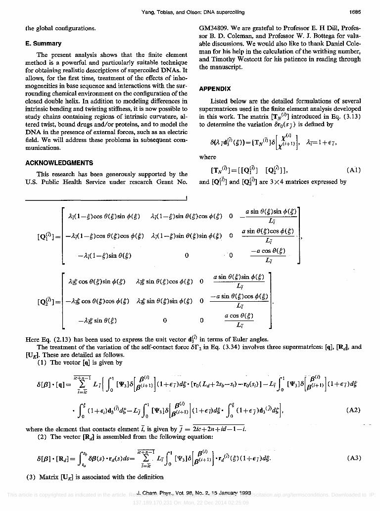
Listed below are the detailed formulations of several supermatrices used in the finite element analysis developed in this work. The matrix [TN(il] introduced in Eq. (3.13) to determine the variation SroCsJ) is defined by

(il S(A id~ilCS»= [TN(il]S[Xt+l)], Ai- 1 +€i,

where

[TN(il ] = [[QVl] [Qfl]], (Al)

and [Q~Tl] and [Qfl] are 3 X 4 matrices expressed by

At< l-s)cos O(s)sin t/JCs) At<I-s)sin OCs)cos t/J(s) 0 a sin OCs)sin ¢lCs)

L~ I

[QVl] = -At< l-s)cos OCs)cos t/J,(s) At< l-s)sin O(s)sin t/J(s) 0 a sin OCs)cos t/J(s)

L~ I

-Aj(1-s)sin OCs) 0 0 -a cos OCs)

L~ I

Ai'S cos OCs)sin ¢I(s) Ai'S sin OCs)cos t/J(s) 0 a sin O(s)sin t/JCs)

L~ I

[Q~Tl] = -Ai'S cos OCs)cos t/J(s) Ai'S sin OCs)sin t/JCS) 0 -a sin OCs)cos t/JCs>

L~ I

-AIS sin O(s) 0 0 a cos O(s)

L~ I

Here Eq. C2.13) has been used to express the unit vector d~Tl in terms of Euler angles. The treatment of the variation of the self-contact force sr 2 in Eq. (3.34) involves three supermatrices: [q], [Rd], and

[UK]. These are detailed as follows. (1) The vector [q] is given by

where the element that contacts element i, is given by] = 2ic+2n+id-l-i. (2) The vector [Rd] is assembled from the following equation:

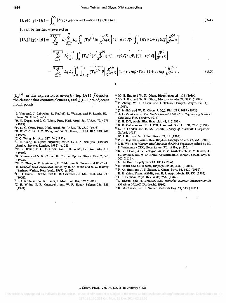
C 3) Matrix [UK] is associated with the definition

J. Chern. Phys., Vol. 98, No.2, 15 January 1993

CA2)

(A3)

This article is copyrighted as indicated in the article. Reuse of AIP content is subject to the terms at: http://scitation.aip.org/termsconditions. Downloaded to IP:

137.189.170.231 On: Mon, 22 Dec 2014 02:25:09

1686 Yang, Tobias, and Olson: DNA supercoiling

[TN(})] in this expression is given by Eq. (AI), J denotes the element that contacts element T, and j, j + I are adjacent nodal points.

I J. Vinograd, J. Lebowitz, R. Radloff, R. Watson, and P. Laipis, Bio­chern. 53, 1104 (1965).

2R. E. Depew and J. C. Wang, Proc. Nat!. Acad. Sci. U.S.A. 72, 4275 (1975).

3F. H. C. Crick, Proc. Nat!. Acad. Sci. U.S.A. 73, 2639 (1976). 4F. H. C. Crick, J. C. Wang, and W. R. Bauer, J. Mol. Bioi. 129,449

(1979). 5 J. C. Wang, Sci. Am. 247, 94 (1982). 6J. C. Wang, in Cyclic Polymers, edited by J. A. Semlyen (Elsevier Applied Science, London, 1986), p. 225.

7W. R. Bauer, F. H. C. Crick, and J. H. White, Sci. Am. 243, 118 (1980).

sR. Kanaar and N. R. CozzareIIi, Current Opinion Strucf. BioI. 2, 369 (1992).

9W. K. Olson, A. R. Srinivasan, R. C. Maroun, R. Torres, and W. Clark, in Unusual DNA Structures, edited by R. D. Wells and S. C. Harvey (Springer-Verlag, New York, 1987), p. 207.

lOCo D. Boles, J. White, and N. R. CozzareIIi, J. Mol. BioI. 213, 931 (1990).

"J. H. White and W. R. Bauer, J. Mol. BioI. 189, 329 (1986). 12J. H. White, N. R. CozzareIIi, and W. R. Bauer, Science 241, 323

(1988).

13M._H. Hao and W. K. Olson, Biopolymers 28,873 (1989). 14M._H. Hao and W. K. Olson, Macromolecules 22,3292 (1989).

(A4)

(AS)

15p. Zhang, W. K. Olson, and I. Tobias, Comput. Polym. Sci. 1, 3 (1991).

16T. Schlick and W. K. Olson, J. Mol. BioI. 223, 1089 (1992). 17 O. C. 2ienkiewicz, The Finite Element Method in Engineering Science

(McGraw-HilI, London, 1971). 18E. H. Dill, Arch. Hist. Exact Sci. 44, 1 (1992). 19B. D. Coleman and E. H. Dill, J. Acoust. Soc. Am. 91,2663 (1992). 20L. D. Landau and E. M. Lifshitz, Theory of Elasticity (Pergamon,

Oxford, 1986). 21W. J. Bottega, Int. J. Sol. Struct. 24, 13 (1988). 22p. J. Hagerman, Annu. Rev. Biophys. Biophys. Chern. 17, 265 (1988). 23 J. H. White, in Mathematical Methodsfor DNA Sequences, edited by M.

S. Waterman (CRC, Boca Raton, FL, 1989), p. 225. 24K. V. Klenin, A. V. Vologodskii, V. V. Anshelevich, V. Y. Klisko, A.

M. Dykhne, and M. D. Frank-Kamenetskii, J. Biomol. Struct. Dyn. 6, 707 (1989).

25M. Le Bret, Biopolymers 23, 1835 (1984). 26H. Tsuru and M. Wadati, Biopolymers 25, 2083 (1986). 27N. G. Hunt and J. E. Hearst, J. Chern. Phys. 95, 9329 (1991). 28E. E. Zajac, Trans. ASME, Ser. E, J. Appl. Mech. 29, 136 (1962). 29c. J. Benham, Phys. Rev. A 39,2582 (1989). 30J. Happel and H. Brenner, Low Reynolds Number Hydrodynamics

(Matinus Nijhoff, Dordrecht, 1986). 31K. Mattiasson, Int. J. Numer. Methods Eng. 17,145 (1981).

J. Chern. Phys., Vol. 98, No.2, 15 January 1993

This article is copyrighted as indicated in the article. Reuse of AIP content is subject to the terms at: http://scitation.aip.org/termsconditions. Downloaded to IP:

137.189.170.231 On: Mon, 22 Dec 2014 02:25:09