final on target
TRANSCRIPT

MEMOIRE
Présenté en vue de l ' ob tent i on du Mas te r en I ngén i eur de ges t ion , à f in a l i t é Advanced Managemen t
Refinancing risk and its impact on distressed company valuation
Romain Hup
Directeur: Professeur Yassine Boudghene Commissaire: Professeur Catherine Dehon
Année académique 2013-‐ 2014

2

iii

MEMOIRE
Présenté en vue de l ' ob tent i on du Mas te r en I ngén i eur de ges t ion , à f in a l i t é Advanced Managemen t
Refinancing risk and its impact on distressed company valuation
Romain Hup
Directeur: Professeur Yassine Boudghene Commissaire: Professeur Catherine Dehon
Année académique 2013-‐ 2014

ii

iii
Abstract The main objective of this dissertation is to develop a model to assess the impact of refinancing
risk on a company value and observe how the latter will react to a refinancing operation. A
literature study of the current credit risk models determines that none of these models are
designed to take this refinancing risk into account. This dissertation therefore presents a model
based on a cash flow approach to value the refinancing exposure of a company. The model
concludes that the refinancing exposure represents a hidden debt for a distressed company. This
hidden debt locks a part of the firm’s value and has a negative impact on both the equity and debt
values of a firm. When a company successfully conducts a refinancing operation that reduces its
exposure, the equity and debt values react positively as the hidden debt decreases. These
conclusions are verified by the study of five distressed companies.

iv
Acknowledgements I would like to express my deep gratitude to Professor Boudghene, my supervisor, for his
guidance and useful critiques of this research work. My grateful thanks are also extended to
Bernard Lalière, Head of High Yield Fixed Income at Petercam Institutional Asset Management,
for his regular feedbacks and valuable support. I also wish to acknowledge the help provided by
the whole Institutional Fixed Income department of Petercam in accessing the financial data
required to write my dissertation. I also would like to thank my parents for the support and
conducive environment they provided me during my whole studies. Finally, my special thanks
are extended to my classmates that made this five years at Solvay so exciting, especially
Florence, Guillaume, Nicolas and Thibaut.
v
Executive Summary When financing their long-term operations by issuing shorter-term debt, companies are required
to refinance their debt on a regular basis and are faced with uncertainty regarding the future
underlying interest rate. This situation, known as refinancing risk, may have an important impact
on the liquidity of a distressed company and might ultimately force it to default. A distressed
company is indeed faced with uncertainty about its future outlooks and will have to pay a
premium when refinancing its debt in order to compensate for the increased risk. Intuitively, this
premium should therefore negatively influence the value of a firm. On the other hand, the latter is
expected to react positively to a refinancing operation.
The goal of this dissertation is to develop a practical model in order to measure the exposure of a
firm to the refinancing risk and ultimately confirm or infirm the intuition regarding the impact of
this risk on a distressed company value. This dissertation will therefore study the refinancing risk
from the perspective of an outside investor. The model presented in this dissertation is based on
the Asset Liability Refinancing Gap model developed by Yann Ait Mokhtar for Exane. However,
due to the little information publicly available, the model has been adapted and completed by the
author.
The methodology used to answer this research question is based on a three-step process. It starts
by a literature review of the existing valuation models and observes whether and how they take
the refinancing risk into account. It then presents a model specifically designed to value the
refinancing risk, the ” Refinancing gap model”, and provides theoretical answers to the research
question. Finally, it applies the model to existing companies and observes whether the theoretical
conclusions are confirmed by reality. Each step of the process relates to a chapter of the
dissertation.
It appears from the literature review that none of the current models takes the refinancing risk
into account when modelling the probability of default of a firm and indirectly its value. As a
matter of fact classical structural models assume that a company defaults as soon as its firm value
falls below a given threshold. Although this threshold depends on the specificities of the model,

vi
structural models rely only on economic distress to trigger off the default of a firm. By doing so,
they fail to take another kind of distress into account, that is to say the financial distress.
Financial distress occurs when the company faces difficulties to honour its financial obligations
and is therefore considered a cash flows or liquidity issue. Refinancing risk is therefore a subset
of this liquidity risk as uncertainty regarding the refinancing terms directly impacts the liquidity
of a firm. As a consequence, classical structural models either assume that the company will be
able to refinance its total debt under the current terms in the future or that the company will stop
existing at the maturity of the outstanding debt. These assumptions are obviously not verified in
reality and require the development of a new model to deal with the refinancing risk.
This new model, called the “Refinancing gap model”, is based on a cash flow approach of the
refinancing risk. In fact the company has to finance its future activities, yielding a known cash
flow, by borrowing at an unknown rate. This situation is similar to a swap position for the
company, in which it receives fixed cash flows from operating activities and has to pay an
interest rate on its future debt that will only be determined when the debt is rolled over. This
swap should be considered an off balance sheet item and is similar to a hidden debt in the case of
a distressed company whose expected refinancing terms have worsened. The value of this swap
represents the exposure of the firm to the refinancing risk. As this exposure is considered a
hidden debt, it directly influences the value of both equity and debt. On one hand, this hidden
debt increases the total leverage of the firm, hence the credit risk of the debt. As a consequence,
the credit spread on the debt will also increase, which will negatively impact the value of the
debt. On the other hand, the hidden debt represents the part of the value of the firm which is
locked due to the refinancing exposure and is therefore currently not available for the
shareholders, resulting in a lower value of the equity. As part of the value of the firm is therefore
locked and not attributed to either the shareholders or the debt holders, the actual value of the
firm, equal to the sum of the equity and he debt value, is lower than the one of a similar firm
without exposure to the refinancing risk.
A distressed company with an exposure to the refinancing risk has various options to reduce this
exposure. These operations (i.e. capital increase, assets disposal, etc) will have a positive impact
on the liquidity of the firm, hence reducing the exposure and the value of the hidden debt. In turn
vii
a reduction in the hidden debt will positively affect the equity and debt value, hence the actual
firm value. On one hand, the reduction in the hidden debt decreases the leverage of the firm and
consequently its credit risk. On the other hand, the refinancing operation will unlock part of the
firm value, which will directly be transferred to the equity.
In theory the refinancing gap model is therefore able to explain how the refinancing exposure
affects a firm value and how the latter reacts to refinancing operations. The model was finally
applied on existing companies to test whether it predicts accurately the equity and debt value of
distressed companies in real terms. It turned out that the refinancing gap model is efficient to
predict the stock price of distressed companies and improves the accuracy of classical structural
models when forecasting the bond spread.
Indeed the refinancing gap model has successfully predicted the stock prices of the four studied
companies presenting a positive refinancing exposure, both before and after the refinancing
operations. Furthermore, it outperformed significantly the classical structural models used as a
benchmark. Moreover, the model successfully predicts the magnitude of the stock price variation
when the firm announces its refinancing operations, which is impossible by means of the classical
structural models. It is clear that these models provide forecasts that are usually contrary to the
stock market reaction. Considering that the refinancing exposure locks part of the value of the
firm to the detriment of the shareholders therefore appears to be a relevant approach. Moreover
this is in line with the stock market reaction to such exposure.
On the other hand, the refinancing gap model systematically predicts bond spreads that are higher
than those of classical structural models, hence improving the accuracy of these models.
Moreover, the biggest improvements appear for companies that face a considerable refinancing
exposure. As a consequence, it proofs that the refinancing risk significantly impacts the bond
spread of a distressed company and justifies partly the “underprediction” of the classical
structural models. However, the Refinancing gap model still fails to accurately predict the real
bond spread and only provides a closer estimation. By considering the refinancing risk in addition
to the economic distress, the refinancing gap model therefore takes into account a wider range of
financial triggers. However, the refinancing gap model does not consider the liquidity issue in its

viii
broad sense. This limitation might explain the remaining difference between modelled and
observed spreads
Following these conclusions about the refinancing gap model as well as its limitations,
improvements to this model can be proposed as future research directions. Firstly, a statistically
significant quantitative study could be conducted to confirm or infirm the results of this
dissertation. Secondly, other proxies for the refinancing premium could be used. Finally, the
accuracy of the refinancing gap model could be improved by trying to include the liquidity risk in
general or by using more advanced, computing-intensive structural models.

ix
Table of contents Introduction ............................................................................................................................................ 1
Chapter 1: Refinancing risk and literature review .................................................................... 4 Section 1: introduction to credit and refinancing risk ........................................................................ 4 1.1 Credit risk measurement ...................................................................................................................................... 5 1.2 Study of default triggers ........................................................................................................................................ 6 1.3 Refinancing risk ......................................................................................................................................................... 8
Section 2: Credit risk modelling .................................................................................................................. 9 2.1 Accounting based models ..................................................................................................................................... 9 2.1.1 Econometrics models ........................................................................................................................................................ 9 2.1.1.1 Altman Z-‐Score ......................................................................................................................................................... 10 2.1.1.2 Econometrics models and refinancing risk ................................................................................................. 12
2.1.2 Credit rating models ....................................................................................................................................................... 12 2.1.2.1 Moody’s methodology ........................................................................................................................................... 13 2.1.2.2 Credit rating models and refinancing risk ................................................................................................... 15
2.2 Market based models ........................................................................................................................................... 15 2.2.1. Market based models and refinancing risk .................................................................................................... 17
Section 3: Structural models ...................................................................................................................... 18 3.1 Merton model .......................................................................................................................................................... 18 3.1.1 Model ..................................................................................................................................................................................... 18 3.1.2 Shortcomings ..................................................................................................................................................................... 21
3.2 Extensions ................................................................................................................................................................. 22 3.2.1 Debt structure .................................................................................................................................................................... 22 3.2.2 First-‐passage model ........................................................................................................................................................ 23 3.2.2.1 Exogenous barrier .................................................................................................................................................. 23 3.2.2.2 Endogenous barrier ............................................................................................................................................... 24
3.2.3 Interest rate process ....................................................................................................................................................... 24 3.2.4 Asset value process ......................................................................................................................................................... 25
3.3 CreditGrades model .............................................................................................................................................. 26 3.4 Accuracy of models ............................................................................................................................................... 28
Section 4: Structural models’ limitations and link with refinancing risk ................................... 29 Section 5: Summary ....................................................................................................................................... 30
Chapter 2: Refinancing Gap model ............................................................................................... 32 Section 1: Presentation ................................................................................................................................ 32 Section 2: Valuation ...................................................................................................................................... 35 2.1 Basic case .................................................................................................................................................................. 35 2.2 Generalization ......................................................................................................................................................... 36 2.3 General framework ............................................................................................................................................... 38 2.3.1 Formulas .............................................................................................................................................................................. 38 2.3.2 Parameters explanation ................................................................................................................................................ 39 2.3.2.1 Refinancing exposure ............................................................................................................................................ 39 2.3.2.1.1 Surplus of cash at t ........................................................................................................................................ 40 2.3.2.1.2 The free cash flows projection of every year .................................................................................... 40 2.3.2.1.3 Dividends paid ................................................................................................................................................ 41 2.3.2.1.4 Interest expenses on outstanding debt ............................................................................................... 41 2.3.2.1.5 Debt payment .................................................................................................................................................. 42 2.3.2.1.6 Refinancing interest expenses ................................................................................................................. 42

x
2.3.2.2 Refinancing premium ............................................................................................................................................ 42 2.3.2.2.1 Expected credit spread ............................................................................................................................... 42 2.3.2.2.2 Risk-‐free rate ................................................................................................................................................... 45 2.3.2.2.3 Cost of debt ...................................................................................................................................................... 46 2.3.2.2.4 Credit premium and tax shield ................................................................................................................ 46
2.3.2.3 Total cost of refinancing ...................................................................................................................................... 47 2.3.2.3.1 Refinancing gap length ............................................................................................................................... 47 2.3.2.3.2 Discounting ...................................................................................................................................................... 50 2.3.2.3.3 Time value ........................................................................................................................................................ 50
Section 3: Company valuation ................................................................................................................... 51 3.1 Merton model .......................................................................................................................................................... 51 3.2 Simplified CreditGrades model ........................................................................................................................ 53 3.3 Complete CreditGrades model ......................................................................................................................... 54
Section 4: Refinancing operations for distressed companies ......................................................... 55 4.1 The case of financially healthy companies ................................................................................................. 57 4.2 Capital increase example .................................................................................................................................... 57
Section 5: Summary ....................................................................................................................................... 61 Chapter 3: Applications of the Refinancing gap model .......................................................... 62 Section 1: Lafarge ........................................................................................................................................... 63 1.1 Description and initial situation ..................................................................................................................... 63 1.2 Refinancing operations ....................................................................................................................................... 66 1.3 Conclusion ................................................................................................................................................................ 68
Section 2: Pernod Ricard ............................................................................................................................. 70 2.1 Description and initial situation ..................................................................................................................... 70 2.2 Refinancing operations ....................................................................................................................................... 73 2.3 Conclusion ................................................................................................................................................................ 75
Section 3: PPR ................................................................................................................................................. 77 3.1 Description and initial situation ..................................................................................................................... 77 3.2 Refinancing operations ....................................................................................................................................... 80 3.3 Conclusion ................................................................................................................................................................ 81
Section 4: TUI AG ............................................................................................................................................ 83 4.1 Description and initial situation ..................................................................................................................... 83 4.2 Refinancing operations ....................................................................................................................................... 85 4.3 Conclusion ................................................................................................................................................................ 88
Section 5: KPN ................................................................................................................................................. 89 5.1 Description and initial situation ..................................................................................................................... 89 5.2 Refinancing operations ....................................................................................................................................... 92 5.3 Conclusion ................................................................................................................................................................ 94
Section 6: Summary ....................................................................................................................................... 95 Conclusion ............................................................................................................................................. 96 Bibliography ....................................................................................................................................... 100 Financial reports and analysis ............................................................................................................... 103
Appendix to chapter 1 ..................................................................................................................... 107 Section 1: Merton model computation ................................................................................................ 107 1.2 Assumptions .......................................................................................................................................................... 107 1.2 Debt and equity valuation ................................................................................................................................ 108 1.3 Credit Spread ......................................................................................................................................................... 110
Section 2: CreditGrades model computation ..................................................................................... 112

xi
Appendix to chapter 3 ..................................................................................................................... 115 1. Lafarge ....................................................................................................................................................... 116 1.1 Assumptions and data ....................................................................................................................................... 116 1.2 Projection of cash inflow / outflow ............................................................................................................. 118 1.3 Refinancing gap computation ........................................................................................................................ 119 1.4 Company valuation ............................................................................................................................................. 120 1.5 Refinancing exposure illustration ................................................................................................................ 121
2. Pernod Ricard .......................................................................................................................................... 122 2.1 Assumptions and data ....................................................................................................................................... 122 2.2 Projection of cash inflow / outflow ............................................................................................................. 123 2.3 Refinancing gap computation ........................................................................................................................ 124 2.4 Company valuation ............................................................................................................................................. 125 2.5 Refinancing exposure illustration ................................................................................................................ 126
3. PPR .............................................................................................................................................................. 127 3.1 Assumptions and data ....................................................................................................................................... 127 3.2 Projection of cash inflow / outflow ............................................................................................................. 128 3.3 Refinancing gap computation ........................................................................................................................ 129 3.4 Company valuation ............................................................................................................................................. 130 3.5 Refinancing exposure illustration ................................................................................................................ 131
4. TUI AG ......................................................................................................................................................... 132 4.1 Assumptions and data ....................................................................................................................................... 132 4.2 Projection of cash inflow / outflow ............................................................................................................. 133 4.3 Refinancing gap computation ........................................................................................................................ 134 4.4 Company valuation ............................................................................................................................................. 135 4.5 Refinancing exposure illustration ................................................................................................................ 136
5. KPN .............................................................................................................................................................. 137 5.1 Assumptions and data ....................................................................................................................................... 137 5.2 Projection of cash inflow / outflow ............................................................................................................. 138 5.3 Refinancing gap computation ........................................................................................................................ 139 5.4 Company valuation ............................................................................................................................................. 140 5.5 Refinancing exposure illustration ................................................................................................................ 141

1
Introduction In November 2008 Standard & Poor’s1 announced that 1,6 trillion euros of European debt would
mature over the next three years in a context of unfavourable bond market conditions. As a
consequence, Standard & Poor’s warned that a growing number of companies might have to
struggle to refinance their debt resulting in a refinancing cost which will be on average 200bp
higher than before August 2007. When financing their long-term operations by issuing shorter-
term debt, companies are indeed required to refinance their debt on a regular basis and are faced
with uncertainty regarding the future underlying interest rate. This situation, known as
refinancing risk, may have an important impact on the liquidity of a distressed company and
might ultimately force it to default. A distressed company is indeed faced with uncertainty about
its future outlooks and will have to pay a premium when refinancing its debt in order to
compensate for the increased risk. Intuitively, this premium should therefore negatively influence
the value of a firm. On the other hand, the latter is expected to react positively to a refinancing
operation.
The goal of this dissertation is threefold: to develop a practical model to measure the exposure of
a firm to the refinancing risk and ultimately confirm or infirm the intuition regarding the impact
of this refinancing risk on a distressed company valuation and finally observe how the latter
reacts to a refinancing operation. In the framework of the dissertation, a distressed company is
defined as a company whose outstanding debt is considered speculative by rating agencies.
Moreover, the company value will be studied from the point of view of the equity (stock price)
and debt (bond spread) values. Finally, a refinancing operation will be defined as an operation
that reduces the refinancing exposure of the company. This dissertation will therefore study the
refinancing risk from the perspective of an outside investor. The approach of this dissertation will
be exhaustive and detailed in order to allow any financial investor to apply the model in practice,
whatever his level of knowledge in credit risk modelling.
1 STANDARD & POOR’S, “Credit Trends: Gaping Refunding Pipeline In Europe Intensifies Financial Challenges“, 2010, p.1.

2
The methodology used to answer this research question is based on a three-step process. It starts
by a literature review of the existing valuation models and observes whether and how they take
the refinancing risk into account. It then presents a model specifically designed to value the
refinancing risk, the ” Refinancing gap model”, and provides theoretical answers to the research
question. Finally, it applies the model to existing companies and observes whether the theoretical
conclusions are confirmed by reality. Each step of the process relates to a chapter of the
dissertation.
The first chapter of the dissertation will start with an introduction of the credit risk and its
measurement. Then it will highlight the different reasons that may trigger off the default of a
company and define one of them, more specifically the refinancing risk. It then presents the
different ways to forecast the credit risk and deep dives into one of them, the structural model. In
this section, the intuition and limitation of the most famous structural models (Merton and
CreditGrades amongst others) will be introduced. Finally, the last section will study whether
structural models take the refinancing risk into account or not.
The second chapter starts by introducing the intuition of the Refinancing gap model and presents
step by step how to apply it, based on a practical framework. It then explains how this refinancing
gap impacts a firm’s value and how to adapt the structural models to take the refinancing risk into
account. Finally, it highlights the different actions that a distressed company can take to solve its
liquidity issues and the impact these have on the company value, in the light of the refinancing
gap.
The last chapter represents the practical implementation of the Refinancing gap model presented
in chapter 2. It will study five companies that all faced an important exposure to the refinancing
risk and decided to use one or several of the refinancing operations introduced in chapter 2 to
reduce this risk. For each company, it will present the background of the firm as well as the
reasons that led to the refinancing exposure. It will also use the refinancing gap model to compute
both the equity and debt values of the firm and compare them with classical structural model
estimations. It will then explain the refinancing operation and compare the predicted outcome (by

3
the refinancing gap model and classical structural model) with the reality. Finally, it extends the
model to a company facing a negative exposure to refinancing risk
Finally, the conclusion presents the limitations of the Refinancing gap model and proposes four
research directions to complement this dissertation and improve the Refinancing gap model.
The refinancing gap model presented in this dissertation is based on a model initially developed
by Yann Ait Mokhtar for Exane and called the “Asset Liability Refinancing gap”. However, as
this model has been developed internally by a financial company, little information is publicly
available. This dissertation is therefore based on the author’s interpretation of the information
available and has been completed by his own research. Moreover, due to the amount of time
required to become familiar with a company history and apply the model in practice, this
dissertation will focus on a relatively limited panel of companies. Therefore this dissertation does
not aim at providing a statistically exhaustive confirmation of the refinancing gap model through
a quantitative study. Instead, it aims at showing the intuition of the refinancing gap models
through relevant cases.

4
Chapter 1
Refinancing risk and literature review
A company with a maturing debt is facing uncertainty about the conditions under which it will be
able to refinance it. This issue, known as refinancing risk, can affect significantly the liquidity of
a company and force it to default. Refinancing risk is therefore a subset of the credit risk. The
goal of this chapter is to present the main models forecasting credit risk, observe how they
potentially take into account the refinancing risk and highlight their limitations.
The first section of this chapter will introduce the credit risk and its measurement. Then it will
highlight the different reasons that can trigger off the default of a company and define one of
them, i.e. the refinancing risk. The second section will present the different ways to forecast the
credit risk while the third one deep dives into one of them, the structural model. In this section,
the intuition and limitation of the most famous structural models will be introduced. Finally, the
last section will study whether structural models take the refinancing risk into account or not.
Section 1: introduction to credit and refinancing risk
When entering into a financial transaction, an investor is facing several risks, the more important
ones being the market risk and the credit risk. The market risk2 is “the risk of a change in value of
a financial asset due to a change in the market conditions (interest and exchange rates amongst
others)”. The market risk is therefore not linked directly with a single company or a financial
product.
On the other hand, the credit risk3 is “the risk that an issuer might default or fail to fulfil entirely
his obligation due to a change in its credit quality”. The credit risk therefore depends on the
2 DARRELL, Duffie and SCHAEFER ,Stephen, Credit Risk: Pricing, Measurement, and Management, Princeton, Princeton University Press, 2003, p.3. 3 ibid.

5
issuer and can lead to large losses for the lender. As a consequence, the latter will require to be
rewarded for his exposure to this risk. This reward will take the form of a premium on the risk-
free interest rate used when there is no credit risk. The premium therefore represents the
compensation for the risk of default and is computed accordingly.
1.1 Credit risk measurement
In order to assess the credit risk of a counterparty, financial regulators have developed several
frameworks. Amongst them, Basel and its subsequent updates are the most famous ones. The
bank of the International Settlements laid down the Basel rules in 1988 to allow all lenders to
measure the possible credit risk in a coherent and similar way and to make sure they have put
aside enough capital to face potential credit losses. This approach has been developed for
financial institutions but can be used by any investor.
Basel defines4 credit risk as:
« The risk of loss from a borrower/counterparty’s failure to repay the amount owed (principal or
interest) to the bank on a timely manner based on a previously agreed payment schedule ».
A more comprehensive definition also includes value risk5:
« The risk of loss of value from a borrower migrating to a lower credit rating (opportunity cost
of not pricing the loan correctly for its new level of risk) without having defaulted ».
In order to model the credit risk, Basel used the following formula6:
EL = PD * EAD * LGD
4 STEPHANOU, Constantinos, and Juan Carlos Mendoza. "Credit risk measurement under Basel II: an overview and implementation issues for developing countries." World Bank Policy Research Working Paper 3556 (2005), p.6. 5 Ibid. 6 ibid.

6
Where:
• EL is the expected loss over a period of time of a financial product or a portfolio
• PD is the probability of default over a period of time
• EAD, or exposure at default, is the amount due to the counterparty at the moment of
default. It is therefore a measure of the extend to which an investor is exposed to the
counterparty in case of a default event
• LGD, or loss given default, is the fraction of exposure that will be lost in the event of
default
While the exposure at default is constantly known for a company, the probability of default and
the loss given default are uncertain and must therefore be predicted by models. In order to
accurately work, these models must take into account all the reasons that may force a company to
default. These reasons are presented in the next section.
1.2 Study of default triggers
According to Davydenko7, several reasons can lead to the default of a firm. He divides them into
two categories: financial and economic distress. Financial distress occurs when the company
faces difficulties to honour its financial obligations. Although the business might seem
fundamentally sound, a temporary decline in cash flows may result in the inability of the firm to
make the scheduled debt payments. On the other hand, economic distress arises when the
prospects of the firm are deteriorating and the value of the business is decreasing. Financial
distress can therefore be seen as a cash flow issue, while economic distress is linked to the value
of a company.
Davydenko observes that at default, most firms are both economically and financially insolvent.
On average, the market value of assets at default is equal to only 60% of the face value of debt.
Moreover, liquidity ratios are below the industry median in 80% of the defaulting firms. He
concludes that8 “persistent economic distress seems to drive financial distress”. Indeed, firms in
7 DAVYDENKO, Sergei A. "When do firms default? A study of the default boundary." A Study of the Default Boundary (November 2012). EFA Moscow Meetings Paper. 2012, p.2. 8 ibid.

7
economic distress are losing money and therefore need to sell their liquid assets to pay the money
back to their creditors and suppliers until they reach financial distress. However, this conclusion
should not be seen as a generality. Low-value firms are distinct from low-liquidity firms in a
substantial amount of observed default events. Around 13% of firms default with low asset value
despite their liquid assets in excess of current liabilities. Furthermore, at least 10% of firms
default, although their asset value is higher than the face value of debt. These firms are therefore
economically solvent, but have major liquidity problems triggering off the default event. Finally,
many distressed low-value and low-liquidity firms are able to postpone default over several
years. Indeed, a majority of economically insolvent companies succeed in delaying the default for
at least a year. Davydenko concludes that neither economic nor financial distress taken alone can
fully explain the default of a company.
Moreover, as different firms default at very different asset values and as there are as many firms
defaulting when their assets are low as the firms that do not, it is hard to define a boundary
separating defaulting from surviving companies. Davydenko and Leland9 both determine the
threshold value “of assets that equalizes the number of defaults above the boundary with the
number of no defaulting firms below it » as being equal to 68% of the face value of debt. Leland
found that structural models calibrated with this threshold generate on average long-term default
probabilities that are in line with the observed data. Although appealing at first glance, the
Davydenko study yields totally different results when companies are analysed on an individual
basis: one-third of defaults occurs at values above this boundary and could not be predicted by
structural models. Moreover, an equal number of companies below it do not default for a least
one year, although the default had been predicted by structural models.
As explained by Davydenko, a transitory liquidity problem can trigger off default, if the firm is
prevented from raising new financing against its assets. If the required amount of cash cannot be
raised, the temporary liquidity issue will force the firm to default, despite its sound economic
fundamentals. In his study, Davydenko10 found that liquidity shortages lead to default only when
9 LELAND, Hayne E. "Predictions of default probabilities in structural models of debt." The credit market handbook: Advanced modeling issues (H. Gifford Fong, Editor) (2006), p.42. 10 DAVYDENKO, Sergei A. "When do firms default? A study of the default boundary." A Study of the Default Boundary (November 2012). EFA Moscow Meetings Paper. 2012, p.8.

8
external financing is hard to obtain due to restrictive covenants or a depressed state of the market
In the absence of such restriction, firms will raise new cash to overcome liquidity shortages as
long as the business remains valuable. Therefore, if external financing is costless, the firm does
not default, except in case of economic distress. Between those two extreme situations, the firm
might be able to raise new financing to face its liquidity issue and refinance its debt albeit under
unfavourable terms. If the company is in a distressed setting, it might indeed have to pay a
premium on its debt. This premium will worsen even more the financial distress of the company
and eventually trigger default sooner than expected.
This problem, known as refinancing risk, is presented in the next section and is a subset of the
credit risk.
1.3 Refinancing risk
Refinancing risk relates11 to the uncertainty regarding the terms and conditions when a company
has to refinance its debt. When the firm issues new bonds to replace the maturing ones, the
market price of the new bonds can be higher or lower than the required principal payments of the
maturing bonds. Depending on the market conditions and the fundamentals of the firm, a profit or
a loss can therefore occur, when the debt is refinanced. In the extreme case, the firm might be
unable to refinance its debt and has to default. The notion of refinancing can be extended to any
need of cash to solve a liquidity issue. This is the uncertainty in general about the cost of issuing
new debt.
Refinancing a debt is also known as rolling it over; hence refinancing risk is also called rollover
risk.
11 HE, Zhiguo, and WEI Xiong. "Rollover risk and credit risk." The Journal of Finance 67.2 (2012), p.5.

9
Section 2: Credit risk modelling
Over the last decades, researchers and practitioners have developed a large number of models to
assess the probability of default of a company. The relevant literature divides these models into
two categories, the ones using accounting information and the others using the market price of
financial assets. These different approaches are presented in the subsection underneath.
Moreover, the limitations of each approach regarding the refinancing risk assessment are
highlighted.
2.1 Accounting based models
2.1.1 Econometrics models
These models12 use data from the financial statements to forecast a company’s bankruptcy risk.
This was originally done through a regression analysis with discriminating factors, but has
recently evolved to Probit and Logit models to define a function S of the form:
S(xi) = β1x1 + β2x2 +… + βnxn
The vector 𝑋 contains the relevant risk factors which depend on the company profile (industry,
privately vs. publicly owned, etc). The table 1 presents an overview of typically used factors in
these models.
12 STEPHANOU, Constantinos, and Juan Carlos Mendoza. Credit risk measurement under Basel II: an overview and implementation issues for developing countries. World Bank Policy Research Working Paper 3556 (2005), p.8.

10
Table 1: Overview of typically used factors in econometrics models13
Information category Parameters
Company type
Industry group
Geography
Age of company
Total sales / assets / equity
Financial Ratios
Equity/assets
Debt/equity
Sales/assets
Profitability
Historical profitability
Profitability growth rate
Profit/ assets
Market data Volatility of stock price
The outcome of econometric models may either be a ranking of the probability of default of
several companies or an assessment of the risk of default of a given company.
2.1.1.1 Altman Z-Score
The most famous of these models is the Z-Score developed by Edward Altman in 1968. The Z-
score is a combination of five weighted business ratios used to estimate the likelihood of financial
distress, as described in the following formula:
13 Ibid.

11
Z = 1.2*T1 + 1.4*T2 + 3.3*T3 + 0.6*T4 + 1.0*T5 where14 :
T1 = Working Capital / Total Assets. It’s a measure of the net liquid assets of the firm relative to
the total capitalization. Shrinking liquidity is a warning sign of financial trouble
T2 = Retained earnings / Total assets. This is a measure of the cumulative profitability of the
company over time
T3 = Earnings Before Interest and Taxes / Total Assets. This ratio is a measure of the true
productivity of the firm’s assets, independent of any tax or leverage factor
T4 = Market Value of Equity / Book Value of Total Liabilities. It’s a measure of how much the
firm’s assets can decline in value before the liabilities exceed the assets and the firm becomes
insolvent.
T5 = Sales/ Total Assets. The ratio is a measure of how effectively the firm uses its assets to
generate sales.
Companies15 with a Z-Score above 2,99 are considered being in the safe zone and thereby not
likely to fall into bankruptcy. Those with a Z Score between 1,8 and 2,99 are located in the grey
area, meaning that their future is uncertain and that there is a chance the company goes bankrupt
within the next two years of operations. Finally, companies with a Z-Score below 1, 80 are in the
distress zone indicating a high probability of bankruptcy over the short term.
The initial formula has been defined by studying publicly traded manufacturing companies.
Altman and other researchers have developed new models to deal with private and non-
manufacturing companies. Moreover, they have continuously updated the parameters of the
model taking into account recent market trends.
In its initial paper, Altman16 claims that the model is 72% accurate in predicting bankruptcy over
a two-year window. Moreover, in 200017, Altman ran subsequent tests and found out that the
14 ALTMAN, Edward I. "Predicting financial distress of companies: revisiting the Z-score and ZETA models." Stern School of Business, New York University (2000), p.10. 15 ALTMAN, Edward I. "Financial ratios, discriminant analysis and the prediction of corporate bankruptcy." The journal of finance 23.4 (1968), p.602. 16 ibid. 17 ALTMAN, Edward I. "Predicting financial distress of companies: revisiting the Z-score and ZETA models." Stern

12
updated versions of the model were accurate in 80 to 90% of the cases to predict bankruptcy over
a one-year window.
2.1.1.2 Econometrics models and refinancing risk
Although none of the famous econometrics models are taking the refinancing risk into account,
these models could be designed to include it. One can indeed add a factor that serves as a proxy
for the refinancing risk such as the credit premium (expected future refinancing rate minus
current one). However, the aim of these econometrics models is not predicting when a firm will
actually go bankrupt, but rather measuring how closely a firm looks like other companies that
have previously filed a petition in bankruptcy. These models therefore fail to predict the
probability of default of a company and can not be used to predict the impact of the refinancing
risk on the value of a firm.
2.1.2 Credit rating models
Credit rating models are models created by rating agencies to assess the creditworthiness of a
company, hence its credit risk level. A rating can either be allocated to a company in general or to
a specific bond in particular and is an indication of the future credit risk of this company or bond.
The credit rating represents the opinion of a particular rating agency about the ability and
willingness of an issuer to meet his financial obligations. Therefore, different rating agencies may
grant a different rating to the same company. There are three major rating agencies: Fitch,
Standard & Poor’s and Moodie’s. Each of them uses a specific grading hierarchy for both short
and long-term obligations. The table 218 shows the correspondence between the three companies
and their meaning.
School of Business, New York University (2000), p.18. 18 BANK FOR INTERNATIONAL SETTLEMENT. “Long-term Rating Scales Comparison.“ www.bis.org. n.d. 24 Mai 2014.

13
Table 2: Comparison of long -‐term credit ratings between agencies and their meaning
Standard & Poor’s
Fitch Moody’s Meaning
AAA Aaa Highest grade credit
AA Aa Very high grade credit
A A High grade credit
BBB Baa Good credit grade
BB Ba Speculative grade credit
B B Very speculative credit
CCC Caa
Substantial risk, near default CC Ca
C
D C Default
Companies with a rating higher or equal to BBB are called “investment grade” companies, while
those with a lower rating are named “Junk, high yield, speculative or non-investment grade”.
2.1.2.1 Moody’s methodology
Each rating agency uses its own methodology to determine the ranking of a given company. The
one developed by Moody’s is based19 on a multi-factor analysis. Moody’s analysts determine a
set of key-factors that fall into two categories: the global, where factors are common to all
companies in any industry and the industry-oriented which are selected to capture the specificity
of a given industry. These factors can be either qualitative or quantitative and are constantly
updated. Quality and experience of management as well as assessment of corporate governance
are some of the global factors. Examples of industry-oriented ones include size and efficiency of
a fleet for the shipping industry. Each factor is subdivided into several sub-factors to which a
particular weight is then allocated. Each sub-factor is calculated for the studied company and is
19 MOODY’S INVESTORS SERVICE. "Rating methodology : Global shipping industry." (2009), p.4-10 passim.
14
allocated a rating factor, based on a mapping grid specific to each sub-factor. Finally, Moody’s
analysts use a last grid to compute the final rating based on each sub-factor weight. Once the
rating has been computed by the analysts, the outcome is presented to the rating committee that
might decide to adjust the rating to take into account company-specific elements that are not
included in the multi-factor analysis, such as regulatory and litigation risk.
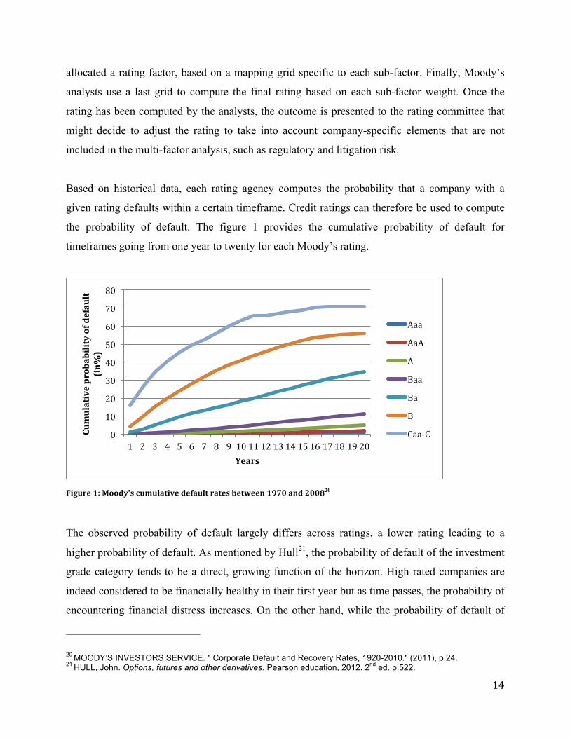
Based on historical data, each rating agency computes the probability that a company with a
given rating defaults within a certain timeframe. Credit ratings can therefore be used to compute
the probability of default. The figure 1 provides the cumulative probability of default for
timeframes going from one year to twenty for each Moody’s rating.
Figure 1: Moody's cumulative default rates between 1970 and 200820
The observed probability of default largely differs across ratings, a lower rating leading to a
higher probability of default. As mentioned by Hull21, the probability of default of the investment
grade category tends to be a direct, growing function of the horizon. High rated companies are
indeed considered to be financially healthy in their first year but as time passes, the probability of
encountering financial distress increases. On the other hand, while the probability of default of
20 MOODY’S INVESTORS SERVICE. " Corporate Default and Recovery Rates, 1920-2010." (2011), p.24. 21 HULL, John. Options, futures and other derivatives. Pearson education, 2012. 2nd ed. p.522.
0
10
20
30
40
50
60
70
80
1 2 3 4 5 6 7 8 9 10 11 12 13 14 15 16 17 18 19 20
Cumulative probability of default
(in%
)
Years
Aaa
AaA
A
Baa
Ba
B
Caa-‐C

15
initially lower rated companies also increases with the horizon, the marginal probability is
decreasing. Hull explains22 this observation by the fact that the first years are critical for initially
unhealthy companies. Once they have survived this trouble period, they will usually recover so
that the marginal probability decreases afterwards. Moreover, the graph shows that probability of
default is always positive whatever the horizon, even short term, except for the highest rated
companies.
2.1.2.2 Credit rating models and refinancing risk
Credit rating models are effectively taking the refinancing risk into account. Rating agencies
indeed look at the refinancing exposure either directly in their model as a global factor or
indirectly by adjusting the rating during the rating committee to reflect the risk. However,
although company rating is an appealing source of information regarding credit risk, one must be
cautious when using it as a prediction of default probability. Such probability is indeed
computed, using a historical set of data comprising companies of similar risk-profile but with a
different history. Moreover, credit ratings are not frequently updated and therefore do not offer
the most up-to-date information. For all these reasons, credit rating models are not efficient to
predict the impact of refinancing risk on the value of a firm.
2.2 Market based models
As previously mentioned, the market-based models use the market price of financial products to
extract the probability of default of a company. There are two different categories of market-
based models, namely the reduced form and the structural one. The differences between both
categories lie in the assumptions regarding information as well as the default trigger.
Reduced form models23 are developed to take into account the sudden nature of a default. Hence,
they consider default an exogenous event driven by a stochastic process. Therefore, they
assume24 that a firm default is an unexpected event, whose likelihood is driven by a default-
22 ibid. 23 WANG, Yu. Structural Credit Risk Modeling: Merton and Beyond. Risk Management 16 (2009). p.30. 24 BENITO, Enrique and Flavan, Silviu. A comparison of credit risk model, Carlos III University in Madrid, March 2005

16
intensity process, such as the Poisson Jump process. 25 Such default intensity process is
extracted26 from the market price of defaultable financial instruments such as credit default swaps
and bonds. As a consequence, the market is the only source of information that reduced form
models use to model credit risk.
Structural models were initiated by Merton in 1974 and aim to provide a relationship between
default risk and capital structure. They assume27 that a company will default when it is unable or
unwilling to meet its financial obligation. The default is thus an endogenous event and will occur
when the assets value of the company will fall below a given threshold. The assets value is
modelled as a stochastic process and the threshold varies according to the structural model
considered.
Structural models therefore assume28 the perfect knowledge of a precise set of information, akin
to the ones held by companies internally. This perfect information assumption therefore implies
that the default is predictable. On the other hand, reduced form models only rely on observable
data from the financial markets. Therefore, the restricted information makes the default
unpredictable. Based on this information, Jarrow and Protter29 claim that the key distinction
between both categories is not the characteristic of the default time (predictable versus
unpredictable) but rather the range of information available. They also show that by reducing or
narrowing the information set available, a structural model can be transformed into a reduced
form one.
The main disadvantage30 of the structural models is their difficulty of implementation. They are
indeed analytically complex and computationally intensive. Reduced form models, on the other
hand, are easy to implement and calibrate, but lag behind regarding their prediction power. In the
25 In probability theory, a Poisson process is a stochastic process that counts the number of events and the time points at which these events occur in a given time interval 26 ELIZALDE, Abel. Credit risk models III: reconciliation reduced-structural models. 2006. p.1. 27 ELIZALDE, Abel. Credit risk models II: Credit risk models II: Structural models. 2005. p.1. 28 JARROW, Robert A., and PHILIP Protter. "Structural vs reduced form models: A new information based perspective." Journal of Investment Management 2.2 (2004). p.2. 29 ibid 30 WANG, Yu. "Structural Credit Risk Modeling: Merton and Beyond." Risk Management 16 (2009). p.32-33 passim.

17
first attempt to compare both categories, Arora and al31 show that structural models constantly
outperformed reduced form ones in both default and spread forecasting.
Moreover, as mentioned by Elizalde32, reduced form models, by relying on exogenous events,
“lack the link between credit risk and the information regarding the firms’ financial situation
incorporated in their assets and liabilities”. They are therefore less able to provide interpretation
to default event.
For these reasons, structural models are widely used in counterparty credit risk analysis and
capital structure monitoring, while reduced-form ones are used on credit security trading floors.
2.2.1. Market based models and refinancing risk
Reduced form models indirectly take into account the refinancing risk when modelling the
probability of default. The default intensity process of these models is indeed extracted from the
market price of defaultable financial instruments. If these financial instruments are correctly
priced by the markets, their spreads should therefore reflect the refinancing risk of the underlying
company. However, as it is impossible to extract from the market price the part of the spread due
to this refinancing exposure, reduced form models do not allow to study the sole effect of the risk
on the firm value. Moreover, as it is impossible to accurately predict the future price of these
defaultable financial instruments, reduced form models are not useful to study the impact of
future refinancing operations.
The link between structural models and refinancing risk will be presented in section 4, following
the presentation of the more famous structural models in section 3.
31 ARORA, Navneet, JEFFREY R. Bohn, and FANLIN Zhu. "Reduced form vs. structural models of credit risk: A case study of three models." Journal of Investment Management 3.4 (2005). p.19-20. 32 ELIZALDE, Abel. Credit risk models III: reconciliation reduced-structural models. 2006. p.1-2.

18
Section 3: Structural models
In this section, the main structural models and their limitation are introduced. Emphasis will be
placed on the rationale behind each model. The goal of this section is indeed to provide intuition
about how they model the probability of default and what are the factors triggering it.
3.1 Merton model
The first structural model was presented by Merton33 in 1974 in a paper that initiated the use of
statistics and mathematics in credit risk modelling. In his paper, Merton develops a framework to
link the asset value of a firm to its credit risk. The assumptions and formulas of the Merton model
are described in appendix 1.1
3.1.1 Model
Merton built his model by considering the easiest financial structure possible for a firm34: At time
t, a given company has assets At, financed by equity Et and zero-coupon debt Dt. This zero-
coupon debt has a face value K and a maturity T > t. Thanks to the balance sheet relationship, the
following equality obtains:
At = Et + Dt
The pay-off at maturity T of the debt will depend on the asset value. When the value of the firm’s
assets at maturity exceeds K, the bondholders receive the full notional amount and the
shareholders receive the residual assets value Vt – K.
On the other hand, when the asset value at maturity is lower than K, the firm cannot face its
financial obligation and defaults. The company is therefore liquidated and the bondholders
receive the firm value Vt , while the shareholders receive nothing. As the shareholders never have
to compensate for the bondholder’s loss, the equity value Et cannot be negative.
33 MERTON, Robert C. "On the pricing of corporate debt: The risk structure of interest rates." The Journal of Finance 29.2 (1974). p.450. 34 WANG, Yu. "Structural Credit Risk Modeling: Merton and Beyond." Risk Management 16 (2009). p.30-31 passim.

19
Figure 2: Schematic representation of the Merton model35
The figure 2 illustrates the dynamics of the Merton Model. Over time, the total debt is constant
and equal to K while the asset value fluctuates. Hence, the total equity value also fluctuates over
time and depends on the asset value. As stated before, the firm will only default, if the firm value
(equals to the total asset value) at maturity falls below the facial amount of the debt, Vt < K. The
facial amount of debt is therefore the default barrier in the Merton Model. One can model the
asset value distribution at maturity by simulating various paths for the asset value process,
following the stochastic diffusion process presented here above. In the Merton model, the
distribution of default is assumed to follow a normal distribution. The shaded area of this
distribution is the probability of default.
Based on these observations, the equity value of the company at time T can be written as 36
ET = max (AT-K ;0).
35 DARRELL Duffie and Stephen Schaefer, Credit Risk: Pricing, Measurement, and Management, Princeton, Princeton University Press, 2003, p.54. 36 SUNDARESAN, Suresh. "A Review of Merton’s Model of the Firm’s Capital Structure with Its Wide Applications." Annu. Rev. Financ. Econ. 5.1 (2013). p.3.

20
This is exactly the payoff of a European call option written on underlying asset AT with strike
price K maturing at T. Similarly, the debt value of the company at time T can be written as37
DT = max (A ; K)
This payoff can be replicated with the following portfolio
DT = K – max (K-A; 0)
In other words, the payoff of the debt at time T is equivalent to holding the face value of the debt
and selling a European put option on the underlying asset AT with strike price K maturing at T.
The figure 3 illustrates the payoff of both debt and equity, depending on the asset value
Figure 3: Equity and debt value as a function of the assets value
37 ibid.

21
The probability of default in the Merton model is therefore given by the probability that the
asset’s value at maturity is lower than the facial value of the debt. In other words, the firm will
default when the shareholder’s call option on the asset underlying matures out-of-money.
3.1.2 Shortcomings
Although appealing on paper, the Merton model suffers, in practice, from a lack of precision in
its predicting power. Van Beem38 studied a panel of Dutch companies and compared the spread
predicted with the Merton model with the market data. He observed that modelled spreads are
zero for short maturities, as solvent companies are not supposed to default on the short term.
However, market data yields a positive credit spread as well as a positive probability of default.
He explained this discrepancy by the Merton assumptions regarding the firm’s asset value
process. As the process follows a slow evolution, the default event can never happen
unexpectedly and the barrier will not be reached within a short period of time.
Moreover, in the long run, credit spread decreases in the Merton model, but is increasing in the
market. This is, one more time, due to the assumptions of this model. According to Merton, firms
cannot issue additional debt before maturity. As the asset value process includes a positive drift39,
the distance between the asset value and the constant facial value of the debt increases and the
firm is less likely to default.
Beside these two observations, Sundaresan40 and Wang41 highlight three more shortcomings of
the Merton model.
Firstly, the debt structure of a firm is nearly always more complicated than a simple zero-coupon
bond. Debt issued by companies often involves intermediary coupons and covenants42.
Secondly, a firm can only default at debt maturity. Therefore, a firm’s asset value can drop below
38 VAN BEEM, J. " Credit risk modeling and CDS valuation :An analysis of structural models." University of Twente (2010). p.22. 39 ibid. 40 SUNDARESAN, Suresh. "A Review of Merton’s Model of the Firm’s Capital Structure with Its Wide Applications." Annu. Rev. Financ. Econ. 5.1 (2013). p.5. 41 WANG, Yu. "Structural Credit Risk Modeling: Merton and Beyond." Risk Management 16 (2009). p.32. 42 A covenant is a promise in an indenture, or any other formal debt agreement, that certain activities will or will not be carried out

22
the facial value of the debt at time t (t < T) and yet recover before maturity. In reality, the firm
would have defaulted at t but not according to the Merton model. The Merton model is therefore
non-path dependant.
Thirdly, the term structure of interest rate observed in reality is not flat, but varies in time, while
the Merton model assumes a constant risk-free rate known with certainty in advance.
3.2 Extensions
3.2.1 Debt structure
As explained before, one of the shortcomings of the Merton model is that the entire debt of a firm
is considered a single zero-coupon bond. This simplified situation is totally unrealistic and firms
usually issue coupon-bearing debt and attach covenants to the debt issues.
Moreover, the usual valuation technique used to price a coupon-bearing bond, which consists in
considering such a coupon-bearing bond as a portfolio of zero-coupons, does not apply to the
Merton model. Indeed, if the firm defaults43 on a coupon payment, then it will automatically
default on all the subsequent payments. The default on one payment is therefore not independent
of the other payment.
A solution to this problem was brought by Geske44. After deriving a formula to price a compound
option45, he observed that the equity of a company with coupon-bearing debt outstanding, could
be considered such an option. Indeed, at every coupon payment date, the stockholders have the
option of buying the next option and keeping the control of the firm by paying the coupon. When
they are unable or unwilling to make the payment, they will default on the debt and the
bondholders will take over the firm and receive the value of the firm. Similarly, at maturity of the
coupon debt, the stockholders have the option to repurchase the claims on the firm from the
bondholders by paying off the principal.
43 MERTON, Robert C. "On the pricing of corporate debt: The risk structure of interest rates." The Journal of Finance 29.2 (1974). p.460. 44 GESKE, Robert. The valuation of corporate liabilities as compound options. Journal of Financial and Quantitative Analysis, 1977, vol. 12, no 04, p. 541-552. 45 A compound option is an option for which the underlying security is another option

23
Although Geske allows considering more complex debt structures than Merton, his structural
model still assumes that the default is expected, as the firm can only default at the coupon or
principal payment dates.
3.2.2 First-passage model
While the Merton model assumes that a firm only defaults when its value at maturity is below the
face value of the debt, in reality a firm can default at any time and for different reasons. The first-
passage models have been created to solve the problem of this limitation, as the firm will default
when its asset value drops below a given default barrier for the first time. These models46 are
therefore path dependant and equity is now modelled as a down-and-out option47. When the asset
value of the company reaches the default barrier, the equity will indeed be worth nothing and the
company will be liquidated. Such default barrier can be seen as a covenant on the debt and
therefore, the value of the debt will be higher than predicted by the Merton model. Similarly, as
default may happen at any time, the probability of pay-off to the shareholders is lower and
therefore, equity will be worth less than according to the Merton model.
The literature offers a wide range of first-passage models that differentiate themselves by their
default barrier specification. They can be classified into two categories: exogenous models that
are defined outside the model and endogenous models, where the barrier is defined inside the
model.
3.2.2.1 Exogenous barrier
The initial first-passage model, created by Black and Cox48 in 1976 included an exogenous
barrier. In such a model, the default barrier is defined outside the model and does not depend on
the shareholders. Black and Cox modelled an exponential safety covenant, which allows the debt
holders to take control of the firm, when this covenant is breached, in other word when the value
of the company is lower than the covenant threshold. The company defaults on its outstanding
46 BLACK, Fischer and COX, John C. Valuing corporate securities: Some effects of bond indenture provisions. The Journal of Finance, 1976, vol. 31, no 2, p. 351-367. 47 A down and out option is an option that ceases to exist when the price of the underlying security hits a specific barrier price level 48 BLACK, Fischer et COX, John C. Valuing corporate securities: Some effects of bond indenture provisions. The Journal of Finance, 1976, vol. 31, no 2, p. 351-367.

24
debt and the shareholders do not receive anything. The value of the default barrier is determined
according to the firm specifics (leverage ratio, credit rating, etc).
Bryis & de Varenne49 modified the Merton model and allowed it to default before maturity. They
used a default barrier that equals the face value of the debt discounted at the risk-free interest
rate. Therefore, the company will default whenever its asset value is lower than the present value
of the face value of the debt.
3.2.2.2 Endogenous barrier
An endogenous default barrier is defined within the model, meaning that the barrier level is
modelled as a shareholders’ decision50. At each coupon payment date, the shareholders decide
whether to pay the debt or not, depending on the prospect of the firm. They will pay only if it
maximizes the equity value in the future. Moreover, they will adapt the endogenous barrier
accordingly. Between the payments, the firm will not default as long as the asset value is higher
than the barrier. The endogenous barrier might be lower than the coming debt payment. In this
case, the firm will not default, although it is not able to service its debt but shareholders will
rather issue equity. The rationale behind this is that shareholders have decided that it is in their
interest to keep the control of the firm thanks to favourable prospects.
Leland51 was the first academician to consider such endogenous barrier in his study on the
optimal capital structure of a company.
3.2.3 Interest rate process
Another limitation of the Merton model presented above is the constant interest rate known with
certainty. The majority of the extensions presented above also make this assumption for the sake
of simplification. However, this assumption is not verified in reality and market observations
show a different interest rate term structure, presenting various shapes and depending on the time,
49 BRIYS, Eric et DE VARENNE, François. Valuing risky fixed rate debt: An extension. Journal of Financial and Quantitative Analysis, 1997, vol. 32, no 02, p. 239-248. 50 VAN BEEM, J. " Credit risk modeling and CDS valuation :An analysis of structural models." University of Twente (2010). p.24. 51 LELAND, Hayne E. et TOFT, Klaus Bjerre. Optimal capital structure, endogenous bankruptcy, and the term structure of credit spreads. The Journal of Finance, 1996, vol. 51, no 3, p. 987-1019.

25
geography, etc.
Several structural models use the stochastic interest rate process of Vasicek to address this issue
and make the interest rate dependent on the time. The Vasicek model is used to describe the
evolution of interest rates using a single market risk. By using stochastic interest rates, these
models are better able to replicate the interest rate term structure, hence leading to more accurate
results. However, a disadvantage52 of the Vasicek interest rate model is that it allows the interest
rate to become negative. It’s therefore of the utmost importance to select the parameter values
properly in order to avoid such situations, as mentioned by Longstaff & Schwartz53.
Nevertheless, using stochastic interest rates adds even more complexity to the structural model,
which becomes harder and longer to process.
3.2.4 Asset value process
All the structural models presented so far use a diffusion process to simulate the asset value of a
firm. Under such diffusion process, the range of possible value taken by the asset value at a given
period of time is limited, making a sudden drop impossible. Therefore, the firm can never default
unexpectedly. As a conclusion, a financially healthy firm has a short-term credit spread equal to
zero, as it cannot default. This conclusion is however rejected by market observations.
The most famous model designed to address this problem was developed by Zhou54 in 1997. He
uses a jump-diffusion process to model the company asset value and therefore allows random
jumps to appear. Therefore, a default can now occur either from the marginal change in the asset
value or from the unexpected shock55. The firm value is then equal to the default barrier in the
first case, but might be below in the second case. Zhou justifies the unexpected jump as being56 «
new important information becoming available to the investors » such as lawsuits or hostile
takeover announcement.
52 FELIX, Jean-Paul. Notes de cours : Marchés financiers en temps continu et modélisation de taux. Université de Picardie, 2010. 53 LONGSTAFF, Francis A. et SCHWARTZ, Eduardo S. A simple approach to valuing risky fixed and floating rate debt. The Journal of Finance, 1995, vol. 50, no 3, p. 789-819. 54 ZHOU, Chunsheng. A jump-diffusion approach to modeling credit risk and valuing defaultable securities, 1997. 55 VAN BEEM, J. " Credit risk modeling and CDS valuation :An analysis of structural models." University of Twente (2010). p.26. 56 Ibid.

26
A structural model with a jump-diffusion process is therefore a combination of both reduced and
structural form models. On one hand, it allows unexpected default events to occur just like in
reduced-form ones. On the other hand, it gives some explanation about the reasons of default,
like structural models do. However, this model requires tough parameter estimation and is
therefore difficult to use in practice
3.3 CreditGrades model
Although appealing in theory, all the models presented above suffer from their complexity when
used in practice. They indeed rely on information that is not readily observable in the market,
such as the asset value and asset volatility. Practitioners therefore need to use proxies to estimate
these required data, resulting in a lack of precision of the models. To overcome this issue, a group
of banks led by Goldman Sachs, Deutsche Bank, JP Morgan and Riskmetrics developed the
CreditGrades model, a model that relies only on observable market data to compute the credit
spread of the debt. This model is based on the first-passage models with exogenous barrier
initiated by Black and Cox but introduces a stochastic barrier instead of a fix one, in this way
solving the issue of null short term credit-spread as explained below.
CreditGrades57 assumes a stochastic process V that follows a geometric Brownian motion, like in
the Merton model. However, in the CreditGrades model, V represents an approximation of the
asset value on a share basis instead of the total asset value. This approximation is equal to the
equity value plus the value in case of default:
V = S + LD
CreditGrades defines default as the first time V crosses the default barrier. This default barrier is
set equal to the recovery value, the amount of the company assets that remain in case of default.
However, empirical studies of recovery rates58 show uncertainty in the recovery value. They
57 FINGER, Christopher, FINKELSTEIN, Vladimir, LARDY, Jean-Pierre, et al. CreditGrades technical document. RiskMetrics Group, 2002, p. 1-51. 58 Hu, H. and Lawrence, L. (2000). Estimating Recovery Rates, JPMorgan document

27
observe an extreme variance of this recovery rate distribution. Not only does it depend on the
industrial sector of the firm, but also on factors such as the default cause (triggered by financial
or operational difficulties) and default outcome (restructuration or liquidation). For this reason,
the default barrier is also assumed to follow a stochastic process. However, the recovery value
may become uncertain over time.
The figure 459 shows how the model works in practice. The default barrier, equal to the recovery
value (LD), varies over time around its initial value. The asset value follows a stochastic process
and as soon as its value falls below the variable barrier, the company will default. By considering
a variable, uncertain default barrier, a firm may default on a really short term. Hence, the credit-
spread is not null at inception. This represents an alternative to the jump-diffusion model
presented above. More information about the CreditGrades model can be found in appendix 1.2
Figure 4: Schematic representation of the CreditGrades model
59 FINGER, Christopher, FINKELSTEIN, Vladimir, LARDY, Jean-Pierre, et al. CreditGrades technical document. RiskMetrics Group, 2002, p. 7.

28
3.4 Accuracy of models
The question of their accuracy has arisen out of the development of structural models and their
growing use by practitioners. In the first study of its kind, Jones & al60 assessed the performance
of the Merton model in practice. They use the model to price corporate bonds and compare the
results with the real data. They conclude that the Merton model has the tendency to
‘underpredict’ the credit spread of a company’s debt. This observation is confirmed by other
studies, led by Eom & al61. In conclusion, the bond value computed by the Merton models is too
high in comparison with the observed one and the model is not accurate enough to be used in
practice.
In their Study, Eom & Al62 decided not only to assess the Merton model but also to compare the
accuracy of different extensions. They test three extensions: Geske (coupon-bearing bond),
Longstaff & Schwartz (exogenous barrier first-time passage), Leland & Toft (endogenous barrier
first-time passage). They observe that all models has the tendency to “underpredict” the observed
spread and therefore present substantial pricing errors. The Geske model is the worst predictor
amongst the four models and underestimates the spread with a mean absolute error of 70%. Using
a stochastic interest rate enables the Longstaff and Schwartz model to show a small increase in
the model, but the spreads are still too low. Moreover, the results are really sensitive to the
Vasicek parameters chosen in the model. On the contrary, in the Leland & Toft model the results
depends on the coupons specification of the bond. These observations do not depend on the credit
quality of the considered company and therefore hold for both investment grade and high yield
firms.
Although the CreditGrades model was created more than a decade ago, few researches have been
properly informed about its accuracy. In 2009 Jaretzke63 conducted the most extensive study to
date involving the CreditGrades model and the only one to include a period of crisis in its sample.
60 JONES, E. Philip, MASON, Scott P., et ROSENFELD, Eric. Contingent claims analysis of corporate capital structures: An empirical investigation. The Journal of Finance, 1984, vol. 39, no 3, p. 611-625. 61 EOM, Young Ho, HELWEGE, Jean, et HUANG, Jing-zhi. Structural models of corporate bond pricing: An empirical analysis. Review of Financial studies, 2004, vol. 17, no 2, p. 499-544. 62 EOM, Young Ho, HELWEGE, Jean, et HUANG, Jing-zhi. Structural models of corporate bond pricing: An empirical analysis. Review of Financial studies, 2004, vol. 17, no 2, p. 499-544. 63 JARETZKE, Dominik. CDS Model and Market Spreads Amid the Financial Crisis. Maastricht University. 2010

29
He observed the spread of 106 North American companies (37 being high-yield and 69
investment grade). He found that CreditGrades model prices the spread reasonably well, although
it has a tendency to underestimate. The model also shows high correlation with the market
spreads. Moreover, the accuracy is better for high-yield obligators than investment grade ones
although the absolute gap between spreads is higher for high yield obligators.
Section 4: Structural models’ limitations and link with refinancing
risk
All the structural models presented in the last section suffer from the same two limitations. These
two limitations explain why the refinancing risk is not taken into account by these models.
Firstly, all the structural models presented in section 3 assumed that the company will be able to
refinance its debt under the same terms as the initial ones. In the end, this assumption is the same
as considering a perpetual debt, as only the coupons are paid, the face value of the debt to be paid
at each maturity being equal to the cash received at the new debt issue64. These models therefore
assume no loss or gain can be made due to the refinancing of the debt. As explained above, in
practice this assumption does not hold, as refinancing exposure can lead to a loss or a profit when
rolling the debt over.
Secondly, the structural models assume that a firm will only default when its asset value fall
behind a given threshold. By doing so, these models only rely on economic distress to trigger a
firm default, without considering the implication of a poor liquidity (financial distress) on the
default event. The refinancing risk in therefore not taken into account as the refinancing exposure
can lead to a liquidity trouble triggering default.
The differences presented in the last section between structural models spreads and reality could
therefore be explained by both the reliance of such models on the sole economic distress to
trigger the default of a company and the assumptions of no loss or gain when rolling the debt
over. By focusing only on the asset value, structural models therefore don’t capture all the
elements provoking a firm’s default.
64 discounting put aside

30
Very few researches have been conducted to overcome this limitation of structural models and
the only model taking into account the refinancing risk has been developed by He and Xiong65.
However, the goal of their paper is to study the market liquidity impact on credit spread and,
although they consider refinancing risk in their approach, their model does not provide a
comprehensive approach for the valuation of such risk. Nevertheless, it provides some interesting
insights about how to approach the issue.
When the firm has to refinance its debt, it will issue new bonds at the current market price, which
can be higher or lower than the required principal payments of the maturing debt. Equity holders
are therefore the « residual claimants » of the rollover gains or losses. Therefore, the net cash
flow to the equity holders is equal to the cash payout of the firm minus the after-tax payment plus
the rollover gain/loss. The rollover gain/loss has a direct impact on the equity cash flow.
Moreover, the model assumes that shareholders issue new equity to absorb the rollover loss,
hence diluting the value of existing shares. As a result, the equity value is jointly determined by
the fundamentals of the firm and the expected future rollover gains/losses. Shareholders will buy
more shares and bail out the maturing debt holders as long as the equity value remains positive.
As soon as it is not the case anymore, the firm defaults and the bond holders take over the firm.
He and Xiong show that equity holders will choose to default at a higher threshold than according
to other structural models, leading to higher credit spread.
This model therefore lacks flexibility as it considers that shareholders automatically issue new
equity to absorb the rollover loss. As a consequence, this model does not allow to study the
impact of refinancing operations on the equity and debt value. Moreover, the model does not
quantify the risk but only uses it to model the spread.
Section 5: Summary
The goal of this chapter was to introduce the refinancing risk and study whether the classical
structural models are taking this risk into account when computing the credit spread of a firm. It
appears that all the widely used structural models rely only on the asset value to trigger off the
default of a firm, without considering the implication of poor liquidity. Structural models are 65 HE, Zhiguo et XIONG, Wei. Rollover risk and credit risk. The Journal of Finance, 2012, vol. 67, no 2, p. 391-430.

31
therefore only able to forecast economic default at the expense of the financial one. The next
chapter will present a model developed by Exane specifically to take the refinancing risk into
account.

32
Chapter 2
Refinancing Gap model In chapter 1, it has been proven that none of the usual structural models were designed to deal
with the refinancing risk. This chapter will therefore present a model, called the “Asset Liability
Refinancing Gap”, which has been specifically created to deal with the refinancing risk. This
model developed by Yann Ait Mokhtar for Exane allows to quantify the risk and compute the
impact of the equity of a firm and debt value.
It will start by introducing the intuition of the model before presenting step by step how to apply
it, based on a practical framework. The second section will explain how this refinancing gap
impacts the value of a firm and how to adapt the structural models to take the refinancing risk
into account. Finally, the last section highlights the different actions a distressed company can
take to solve its liquidity issues and the impact they have on the company value, in the light of
the refinancing gap.
The approach followed to compute the refinancing risk exposure is based on the Asset Liability
Refinancing Gap model (ALRG) developed by Yann Ait Mokhtar for Exane. However, as this
model has been developed internally by a financial company, little information is publicly
available. This dissertation is therefore based on the author’s interpretation of the information
available and has been completed by his own research.
Section 1: Presentation
Yann Ait Mokhtar, head of quantitative research at Exane, has developed another approach to the
rollover issue66. He observed that the classical structural models failed to predict the stock
behaviour of distressed companies trying to avoid bankruptcy. He explained theses discrepancies
by the assumptions made regarding the debt. As highlighted before, all structural models assume
that the company has the possibility to refinance its debt at the present conditions at any time in
the future. 66 EXANE BNP PARIBAS, Capital Structure Optimization : CDS and share price, ALRG model and country risk, 2013

33
However, the future financing terms are not currently known. Therefore, the company has to
finance its future activities, yielding a known cash flow, by borrowing at an unknown rate67. This
situation is similar to a swap position for the company, in which it receives fixed cash flows from
operating activities and has to pay an interest rate on its future debt, that will only be determined
when the debt has been rolled over. This swap should be considered an off- balance sheet item
and is similar to a hidden debt or a hidden receivable, depending on the sign. Ait Mokhtar calls
this swap “the refinancing gap or the asset liability swap”.
The firm’s value must therefore be adjusted to include this hidden debt/receivable, which is
added/subtracted to the sum of the equity and debt values. The rationale behind this is that the
current equity and debt are not sufficient to allow the company to meet its full operating potential
in the future. In order to reach this full potential and therefore receive all the predicted cash
flows, the firm will have to refinance its debt in the future. If it does not, the company might
come short of cash and face liquidity issues. This hidden debt therefore locks a part of the firm
value which is not available for neither shareholders or bondholders. However, the classical
valuation models only take into account the current debt and the equity market expected value
and do not consider the impact of future refinancing.
If the firm is able to borrow under the same terms in the future as the current ones, there is no
refinancing gap and the classic equality applies.
However, if the financing terms worsen in the future, the company will have to pay a higher
interest rate on the refinanced debt. It will therefore be costlier for the firm to keep its business
operating and the refinancing gap value will be positive. The current debt value must therefore be
adjusted to take this higher cost into account. As a consequence, the debt and equity value are
negatively impacted. This situation is illustrated on the figure 5.
67 EXANE, The Asset Liability Refinancing Gap model : Valuation and Arbitrage of indebted companies, January 2009

34
Figure 5: Firm value breakdown when positive refinancing exposure
On the other hand, when the refinancing terms improve in the future, the firm will borrow at a
lower interest rate on the refinanced debt. It will therefore be cheaper for the company to operate
the business and the refinancing gap value will be negative. This refinancing gap is therefore
considered a receivable for the company and will increase the current firm value. In fact, the
latter does not take into account this improvement and is only based on equity and debt market
value. This situation is illustrated on the figure 6.
Figure 6: Firm value breakdown when negative refinancing exposure

35
By doing so, the current debt value is adjusted to take into account the future expected cost or
gain on the debt, hence reflecting a more accurate view of the company.
Section 2: Valuation
In this subsection, the refinancing gap valuation rationale will be introduced step by step. It will
start with an overly simplified case that will present the intuition behind the refinancing gap
valuation. Then, a generalized example will be used to emphasize the main factors influencing
the value. Finally, a complete framework will be detailed. The goal of this framework will be to
highlight the required information as well as the different steps to value the refinancing gap.
2.1 Basic case
The following example applies to an overly simplified company and is used to explain the basics
of the refinancing gap valuation.
Company X will receive a single free cash flow of 150€ after ten years. This company is
financed partly by a coupon bond with a face value of 100€ and a maturity of five years. The
company currently pays 2% interest on its debt. If the company wants to receive the free cash
flow, it will have to survive until year 10, meaning that it will have to refinance its debt, in year 5
and this for five more years. However, the debt is expected to be more expensive in the future
and the current estimate (five year forward rate in five years) is 4%. Company X will therefore
pay an extra 2% interest rate on its debt for the last five years of its existence, which is equal to
2€ per year or 10€ in total. The value of the refinancing gap is thus equal to 10€ (without taking
discounting into consideration).

36
Figure 7: Cash flows illustration
The refinancing gap value can therefore be approximate to the following formula:
Refinancing gap = credit premium * Time * Face value of debt
2.2 Generalization
This second example represents a more realistic company and is used to show the main factors
influencing the refinancing gap value.
Company Y currently has 500€ in cash on its bank account. It receives a known after-coupon free
cash flow of 100€ every year. It is partly financed by debt and has two outstanding coupon bonds
with maturity of respectively three and five years and a coupon rate of 2, 5% paid annually. The
face value of both bonds is respectively 1200€ and 600€. Company Y therefore pays 40€ interest
per year on the outstanding debt. It uses the yearly free cash flow to meet this financial obligation
and has a cash increase of 100€ at the end of each year.
As shown on figure 8, the increase in cash over the years can be represented as a rising line. Until
year 3, the firm does not have to pay back any debt and is accumulating cash. In year ,3 the first
principal payment of 1200€ is due. However, the company has only 800€ cash in reserve and

37
therefore must borrow 400€ to pay to its creditors. In year 4, the company receives its annual
after coupon free cash flow of 100€ and has no principal payment due during the year. It will
therefore use this cash to partially buy back the new debt issued the year before. The outstanding
debt is thus equal to 900€ (600€ of old debt maturing in year 5 and 300€ on debt issued in year
3). In year 5, the second principal payment is due and the firm will pay 600€ to its creditors. As
the company only has the yearly free-cash flow in reserve, it will borrow 500€. The total debt
outstanding has thus a face value of 800€. As of year 6, the company will use its yearly increase
in cash to buy back a part of the debt until year 13 when the newly issued debt will be fully paid.
The company therefore has chosen the maturity of the new debt accordingly. The first debt of
400€ issued in year 3 will have a maturity of 10 years and the second debt of 500€ issued in year
5 a maturity of 8 years.
Assuming that the credit spread is forecasted to increase to be equal to 3, 5% for all maturities,
the company will pay a credit premium of 1% on the future debts. The extra financing cost due to
credit-spread increase is therefore equal to 43€ (without taking discounting into consideration).
The new formula to price the refinancing gap is:
outstanding debt ∗ credit premium
Figure 8: Refinancing exposure illustration
It is important to note that this example considered the after-coupon free-cash flow. Therefore, all

38
considerations regarding the interest rate were not taken into account. In reality, the firm will
have to pay a higher interest rate on the new debt, impacting the cash available. For simplicity
purposes, this example assumed that the cash available for the company was constant whatever
the interest rate.
2.3 General framework
In order to generalize the previous example and compute the refinancing gap for any company,
we developed a practical framework. This framework shows in three steps how to value the
refinancing gap at time t=0. All the parameters used in the formulas are then presented
exhaustively.
2.3.1 Formulas
The first steps consists in computing the refinancing exposure or the amount to be refinanced on a given year t: 𝑅𝐸! = − 𝐸𝑅𝐶𝐹!!
!!! + 𝐶𝑎𝑠ℎ! Where: 𝐸𝑅𝐶𝐹! is the equity residual cash flow net of dividend payments 𝐸𝑅𝐶𝐹! = 𝐹𝐶𝐹!! − 𝑖𝑛𝑡.𝑝𝑎𝑦𝑚𝑒𝑛𝑡𝑠 ∗ 1− 𝑡! –𝑝𝑟𝑖𝑛𝑐𝑖𝑝.𝑑𝑒𝑏𝑡 𝑟𝑒𝑝𝑎𝑦𝑚𝑒𝑛𝑡𝑠 − 𝑑𝑖𝑣𝑖𝑑𝑒𝑛𝑑 t! is the effective tax rate at t=0 Cash! is the treasury at t=0 Then, one must compute the credit premium at t=0 or the additional interests rate that a company will pay when refinancing its debt comparing to the current one 𝐶𝑃! = − 1− 𝑡!! ∗ 𝑘!!! − 𝑟!! + 𝐶𝐷𝑆! Where: 𝑘!!! is the cost of debt at t=-1 𝑟!! is the risk-free rate at t=0

39
𝐶𝐷𝑆! is the M-year CDS spread M is the weighted average maturity of the outstanding debt at t=0 The last step consists in computing the total cost of refinancing or refinancing gap at t=0
RG! =!"!∗!"!!!!!
! !!!!! ∗ !
!!!!!
Where: T is the first year the refinancing exposure becomes negative P!! is the M-year probability of default of the company
2.3.2 Parameters explanation
2.3.2.1 Refinancing exposure
As explained in the second example the amount to refinance is not equal to the facial debt which
is due in a given year. The company will indeed use its cash reserve rather than borrowing to
cover the debt payments.
As explained in the previous example, the framework assumes that any surplus of cash in a given
year will be used to buy back part of the outstanding debt. The framework is therefore dynamic
and relies on the assumption that debt can be bought back at any time. As a consequence, the
framework computes the net shortage of cash in every year.
It is therefore required to compute the amount of cash available on every year in the future as
well as the outflow of cash due to the debt. This is equal to the equity residual cash flow net of
dividend payments. Six parameters are required to compute it.

40
2.3.2.1.1 Surplus of cash at t
The surplus of cash at t: Over the past years the company might have accumulated a reserve of
cash and other very liquid assets such as treasury bills, commercial paper and money market
holdings. This cash is available in case of emergency or to avoid having to refinance the debt
entirely. In order to find the amount of surplus of cash at t, one must look into the annual report
of the company and look for the “cash and cash equivalent” account on the balance sheet.
2.3.2.1.2 The free cash flows projection of every year
Every year the company will have a net cash inflow or outflow that will increase or decrease its
initial cash reserve. This net cash inflow or outflow is equal to the free cash flow of the company,
which represents the total cash received or given in the day to day operations of the company
(operating cash flows) as well as the cash spent in the investment (investing cash flows). These
free-cash flows are usually forecasted by the financial analysts over a period of time going from
three years to ten years, with an average of five years. When no more projections are available, it
is usual to assume a constant annual growth rate of the free-cash flows.
The surplus of cash and free cash flow projections must however be carefully considered when
the company presents consolidated accounts. Indeed, in these consolidated accounts, the
company will include all the assets of its subsidiaries, liabilities and equity into its own account
according to the full consolidation method, provided it has control over these subsidiaries68.
Nevertheless, the company does not have a direct claim on the cash reserves of its subsidiaries
which therefore cannot be included in the refinancing gap computations. Moreover, the same
issues arose until recently for joint-ventures, in which a company was involved and which was
included into the company’s financial accounts using the proportionate method. According to this
method, the assets, liabilities and equity of a joint-venture were included in the financial
statement of the company proportionally to its stake in the company. This method is not used
anymore but one should pay attention to it while applying this framework in the past. The current 68 Control is presumed to exist when the parent company: holds, directly or indirectly, over 50% of the voting rights in its Subsidiary; holds, directly or indirectly less than 50% of the voting rights, but has power over more than 50% of the voting rights by virtue of an agreement with other investors; has power to govern the financial and operating policies of the Subsidiary under a statute or an agreement; has power to cast majority of votes at meetings of the board of directors, or has power to appoint or remove the majority of the members of the work all the cash available, by acquiring securities.
41
method, namely the equity method, which is also used when a company owns between 20% and
50% of another one, consists in reporting proportionally the net income of this other company in
its own annual account and therefore presents the same risks. One must therefore analyse
carefully the financial accounts and look into the notes to be sure not to take into account the
information relating to the subsidiaries and other investments.
2.3.2.1.3 Dividends paid
Although the free-cash flow represents the net cash inflow or outflow of a company, all this cash
is not saved by the company. The latter might indeed decide to distribute part of this cash to its
shareholders. The last parameter to determine the amount of cash available every year is therefore
the dividend policy of the company. These numbers are usually forecasted by the financial
analysts just like the free-cash flow. When no projections are available, two options are possible.
One can either compute the ratio dividend per free cash flow and apply it to the future FCF or
apply a constant annual growth rate to the current dividend.
2.3.2.1.4 Interest expenses on outstanding debt
As the free cash flow used in this framework represents the net cash inflows or outflows of an
unlevered company, it does not take into account the interest expenses due on the outgoing debt.
These expenses must therefore be taken into consideration and can either be subtracted from the
accumulation of cash or added to the debt. In this framework, a simplified approach is used to
deal with interest expenses. The first step is computing the weighted average interest rate on the
issued debt. This average is computed by taking the respective face value and interest rate of
every outstanding debt. The weighted average interest rate is then applied to the outstanding debt
on a given year to find the interest expenses of this year. The amount of debt outstanding
decreases over time as part of it comes to maturity. A table including the information for every
debt issue can usually be found in the appendixes of the annual report. As these interest expenses
are not taken into account when projecting the free cash flow, one must consider the interest tax
shield on the outstanding debt. The company may indeed deduct these expenses. This framework
will therefore consider the after tax interest rate. The effective tax rate tc can be found in financial
analysts’ reports.

42
2.3.2.1.5 Debt payment
The company will have to pay back the face value of all the outstanding debt according to the
repayment schedule. This repayment schedule is usually included in the appendixes of the annual
report. In this framework, the convertible debt is considered a regular debt and is therefore not
assumed to be exercised and converted into equity by the holders.
2.3.2.1.6 Refinancing interest expenses
Finally, the company will also have to pay interests on the debt issued to finance the refinancing
gap. These interests will substitute to the interest expenses on the outgoing debt as soon as part
of it comes to maturity. These refinancing interest expenses are computed each year by applying
the refinancing interest rate to the refinancing gap (see below for more explanation). 69 The
refinancing interest rate used is the after tax one, for the same reason as in the interest expenses
on outstanding debt.
2.3.2.2 Refinancing premium
As explained before, the terms under which the company will finance this gap in future are
unknown at the time of the valuation. However, it is likely than these terms will be different from
the ones on the maturing debt. If the new debt is cheaper to issue, the company will book a virtual
profit, whereas it will lose money if the debt becomes more expensive. In order to compute this
gain/loss, one must compute the refinancing premium. This premium is defined as follows : the
difference between the average interest rate on the maturing debt and the expected interest rate on
the debt when the refinancing occurs.
2.3.2.2.1 Expected credit spread
However, this expected interest rate cannot be determined with certainty before the rolling over
of the debt and a proxy must therefore be used to approximate it. Two different methods can be
69 As the refinancing interest expenses requires the refinance gap value to be computed and the refinancing gap requires the refinancing interest expense, a problem of circularity arises. Therefore, it’s required to use a spreadsheet application to apply the framework

43
used in this framework to compute the proxy: the first one consists in using the yields70 on the
outgoing traded debts of the company. The second one relies on the CDS71 prices quoted on the
debt of the firm.
In theory72, both methods should give the same results as the CDS spread is supposed to be equal
to the bond spread for the same borrower and maturity. This equality comes from the non-
arbitrage assumptions and can be justified by considering the following portfolio: a long position
on a bond and a long position on a CDS quoted on this bond. As the CDS will hedge the default
risk of the bond, this portfolio is equivalent to a risk-free asset. The return on this portfolio,
which is equal to the bond yield y minus the CDS premium c, is therefore equal to the risk-free
rate r:
y – c = r or c = y- r
By definition, the CDS spread is thus equal to the bond spread. If it is not the case, an arbitrageur
should be able to gain some benefit from this situation and earn a certain profit without taking
any risk. The choice of the risk-free rate is therefore of the utmost importance when comparing
bond and CDS spread, as different risk-free instruments will yield different spreads and hence
different arbitrage opportunities. This issue will be developed in the next subsection.
However, in reality, discrepancies are observed when comparing both spreads. Several reasons
explain these discrepancies and are highlighted in a study from the National Bank of Belgium73:
- Market premium: Corporate bond markets are often less liquid than the CDS, which
explains why a liquidity premium is observed in the bond, yields. Studies show that the
CDS spread incorporates a lower liquidity premium than the bond spread, resulting in a
smaller CDS spread. The greater liquidity of the CDS market can be explained by several
70 Yield : in this case, the yield to maturity. It’s the total return an investor will receive if he holds the bond to maturity 71 The credit default swap, or cds, is a swap designed to transfer the credit exposure of fixed income products between parties 72 HULL, John, PREDESCU, Mirela, et WHITE, Alan. The relationship between credit default swap spreads, bond yields, and credit rating announcements. Journal of Banking & Finance, 2004, vol. 28, no 11, p.10. 73 DE WIT, Jan. Exploring the CDS-bond basis. National Bank of Belgium, 2006. p.7-13
44
reasons74. Firstly, an investor who wants to liquidate its CDS position does not have to
sell it on the market, but can draw up a contract on the same CDS in the opposite
direction. This is not possible for bonds. Secondly, there is no limit in the amount of CDS
contracts that can be traded as supply is unlimited. Thirdly, the CDS market on a given
underlying company is not fragmented as the bond market. Indeed, the latter is made up
of successive issuances. Finally, CDS sellers are more active in the market while part of
bond investors purchase bonds as part of a “buy and hold” strategy. Several studies
consider market premium the highest source of discrepancies.
- Accrued interest: In case of default, a bond does not generally pay accrued interest to
bondholders. On the other hand, under standard CDS contract, the buyer has to pay the
accrued premium up to the credit event.
- Cheapest to deliver bond: In the case of physical delivery after a credit event, the buyer is
generally free to choose the bond he wants to deliver from a basket of deliverable bonds.
He will therefore choose the cheapest to deliver one, giving him a delivery option. Since
CDS sellers will likely end up with the least favourable bonds, if the different deliverable
bonds are trading at different spreads, they must be compensated by a higher premium for
the risk they are taking.
- Counterparty risk: The two parties in a CDS contract bear exposure to each other’s ability
to fulfil their respective obligations. The risk is limited to the premium payment for the
CDS sellers. However, the buyer faces greater uncertainty as the seller could default and
therefore might not be able to pay the buyer, should the underlying company default, too.
The difference between par and recovery value is therefore at stake. CDS buyers will tend
to accept to pay a lower premium to take the counterparty risk into account.
Moreover, several studies, amongst which Blanco & al75 and Coudert & Gex76, have analysed
the long-run relationship between CDS and bond spread. They found out that the CDS market
is leading the bond market, meaning that CDS spreads are adjusting more quickly to new
74 COUDERT, Virginie et GEX, Mathieu. Credit default swap and bond markets: which leads the other. Financial Stability Review, Banque de France, 2010, vol. 14, no 2010, p.163. 75 BLANCO, Roberto, BRENNAN, Simon, et MARSH, Ian W. An empirical analysis of the dynamic relation between investment‐grade bonds and credit default swaps. The Journal of Finance, 2005, vol. 60, no 5, p.28. 76 COUDERT, Virginie et GEX, Mathieu. Credit default swap and bond markets: which leads the other. Financial Stability Review, Banque de France, 2010, vol. 14, no 2010, p.3-4.

45
information than bond spreads do. Informed traders are indeed more likely to turn to the CDS
market because of the highest liquidity as explained before.
In this framework, we have opted to use the CDS spread to estimate the future refinancing
cost. The highest liquidity of the CDS market combined with its swifter reaction to new
information makes CDS spread a better estimator than the yield spread. Moreover, the
fragmentation of the bond market due to the successive issuances would make the study of
bond spreads more complicated.
The maturity of the CDS will depend on the rollover policy selected. When no data are
available for the corresponding CDS maturity, one will usually infer it from the maturity
available on the market, using linear approximation. For a non-negligible amount of
companies, the only quoted CDS maturity is 5 years. Given that the average debt maturity is
often close to 5 years, using the 5-year CDS is a reasonable approximation.
2.3.2.2.2 Risk-free rate
Once the credit spread has been computed, the next step consists in computing the forecasted
interest rate, which is equal to the sum of the credit spread and the risk-free rate. In recent
years the choice of the risk-free rate has been at the heart of a large debate between
practitioners and academicians. The government bond has been the reference for a long time.
The rationale behind this choice77 was that a bond issued by a government in its own currency
has no credit risk and therefore its yields must be equal to the risk-free rate. However, the
yield on government bond tends to be much lower than the yield on other zero or very low
credit risk instruments. Hull78 explains this lower yield in the case of the US Treasury bond
by three elements. Firstly, the financial institutions have to use the treasury bills to fulfil a
variety of regulatory requirements. Secondly, a financial institution has to hold substantially
less capital to support an investment in Treasury bonds than the capital required to support a
similar investment in low risk corporate bonds. Finally, interest on Treasure bonds is not
taxed at the state level, whereas interest on other fixed income investments is. These three
77HULL, John C., PREDESCU, Mirela, et WHITE, Alan. Bond prices, default probabilities and risk premiums. Default Probabilities and Risk Premiums (March 9, 2005), 2005. p.3. 78 Ibid.

46
reasons explain why US financial institutions hold a large amount of Treasury bonds and
therefore allow the US treasury to issue bonds at a lower interest rate. The same reasoning
applies to government bonds from other countries.
Recently professionals have given up government bonds to use the swap zero curve79. This
curve is usually computed using Libor, deposit rates and swap rates. The rates for maturities
less than one year are Libor deposit rates. They represent the short-term rates at which a
financial institution is willing to lend funds to another financial institution through the
interbank market. The borrowing institution must have an acceptable credit rating defined as
a rating higher or equal to Aa. Longer rates are tougher to comprehend. Hull defines the n-
year swap rate as “the rate of interest on an n-year loan that is somehow structured so that the
obligator is certain to have an acceptable credit rating at the beginning of each accrual period.
Therefore, the rates calculated from the swap zero curve are very low risk rates but are not
risk free. They are also liquid rates that are not subject to special tax treatment. »
In this framework, the 10-year swap rate in the main currency of the company will be used.
2.3.2.2.3 Cost of debt
The cost of debt is assumed to be equal to the interest rate on the most recent debt issued by the company
2.3.2.2.4 Credit premium and tax shield
As mentioned before, an indebted company is allowed in many countries to deduct its interest
expenses, hence lowering the amount of taxes to be paid. This mechanism is known as the
interest tax shield. As the company’s future interest rate has changed, so has the interest tax
shield. A company that must pay a 1% premium on its debt in the future will indeed increase
proportionally its tax shield, hence lowering the effective refinancing cost for the company. The
credit premium must therefore be adjusted to take the tax shield into account and is equal to:
79 HULL, John, PREDESCU, Mirela, et WHITE, Alan. The relationship between credit default swap spreads, bond yields, and credit rating announcements. Journal of Banking & Finance, 2004, vol. 28, no 11, p.12.
47
Effective tax premium = (1-tc) * computed tax premium
The same reasoning applies for the negative tax premium: the company will pay a lower interest
rate in the future, hence a lower tax shield. The company gain must therefore be adjusted to take
this loss in tax shield into account.
2.3.2.3 Total cost of refinancing
2.3.2.3.1 Refinancing gap length
The company will have to refinance its debt as long as its cumulative debt payments are higher
than the cumulative accumulation of cash. It means that the company will borrow money until it
has enough cash to pay back its entire debt and to finance its operation only by means of its free
cash flows. An alternative explanation is to consider that the company will stop rolling over its
debt as soon as the cash surplus released by its operations is sufficient to pay back all its debt.
Once the gap length has been determined, one has to decide the rolling over policy that is to be
applied. Two options are considered in this framework.
The first one consists in assuming that the debt is rolled over at a given frequency. This
frequency is equal to the current average maturity of the debt. By doing so, the framework
assumes that the company is not changing its debt management policy and is simply rolling over
its maturing debt over the average maturity of its entire debt. This method also assumes that the
future refinancing terms will be equal to the one of the first rolling over. In reality, this
assumption only holds, if there is no new information that might change the refinancing terms in
the future.
The second option assumes that the debt financing the yearly cash deficit has a maturity equal to
the end of the refinancing gap. The rationale behind this approach is that, as the company knows
when it will be able to operate without additional debt, the easiest way to refinance its maturing
debt is to choose a maturity equal to the end of the refinancing period. By doing so, it will not be
necessary to refinance again the debt in future and there is therefore no longer any refinancing
risk, as all the terms have been fixed now. The maturity of the future new debt issue will

48
therefore decrease over the years, as the end of the refinancing gap is getting closer. However,
this method requires computing the refinancing premium for different maturities while the first
one only requires one computation.
The following example highlights the differences between both methods.
Company X has the following outstanding debt: 100€ maturing in 3 years and 200€
maturing in 6 years. According to the framework, it will face a refinancing gap for the
next 12 years. It is assumed that no other cost related to the debt is to be financed in the
future.
According to the first method, the weighted average maturity of the outstanding debt is
equal to 5 years. Therefore, the 100€ will be refinanced in 3 years for 5 years. Then, in 8
years, the company will once again roll over the 100€ until year 13. As the refinancing
gap will have disappeared by year 12, the company will have paid back the 100€ one year
earlier than scheduled (year 12 instead of year 13). Similarly, the 200€ will be refinanced
in year 5 and then in year 10. It will be paid back after two years, therefore three years
ahead of schedule. This process is illustrated on figure 9.
The second method assumes that the 100€ will be refinanced only once by a new debt of
maturity of 9 years and the 200€ with a new debt of maturity of 7 years as shown on
figure 10.

49
Figure 9: Fixed frequency debt rolling over illustration
Figure 10: End of gap debt rolling over illustration
The difference of outcomes between both methods will depend on the expected interest rate curve
shape of the company. If the curve is flat and the interest rates constant for both maturities, both
methods will give the same results. In the case of an upward slope, the method using the lowest
maturity will yield a lower refinancing cost. In the case of distressed companies, the gap length is
usually higher than the average maturity on the outstanding debt and therefore the first method
will be favoured by companies, as the refinancing cost will be lower. The situation is exactly the
opposite when the curve is downward sloping.

50
In the case of distressed companies, the interest rate curve is generally downward sloping as there
is considerable uncertainty about the ability of the company to survive in the short term. It might
therefore be efficient for the distressed company to issue long maturity debt in order to benefit
from the lower interest rate. However, it is very unlikely that the distressed company will be able
to successfully issue a debt with a long maturity and a high face value. The market will indeed be
reluctant to invest on the long run in a company with negative financial perspectives.
This framework will favour the first method both for practical reasons as well as for financial
accuracy.
2.3.2.3.2 Discounting
Given that the refinancing gap is considered a hidden debt, this framework will use the cost of
debt (Kd) as the discount factor.
2.3.2.3.3 Time value
The refinancing gap value computed previously is based on the assumptions that the future free
cash flows are known and certain and that the debt refinancing occurs immediately after the need
appears. However, the refinancing, although required, might be delayed and there is some
uncertainty regarding the free cash flows projection. As a consequence, the refinancing gap value
includes a “time value”, just like an option does, which accounts for the uncertainty. This time
value is difficult to quantify and this framework will use a proxy in the form of the default
probability of the company. As a matter of fact the probability of default depends on the free cash
flow expectation as well as on the refinancing or not of the debt and therefore encompasses both
parameters of the time value. The rationale behind the use of the probability of default is that the
framework only computes a value as long as the company does not default. As soon as the
company defaults, there are no more free cash flow projections nor any refinancing risk and the
refinancing gap value is therefore nil. However, one cannot predict the default occurrence when
computing the refinancing gap value and adapt the results as a consequence. This framework
therefore proposes to correct the refinancing gap value by taking the probability of default into
account, hence the time value.

51
A company with a probability of default equal to 20% will therefore have a time value equal to
1/0,8 = 25% on the intrinsic refinancing gap value. The final refinancing gap value is therefore
equal to 125% of the intrinsic one. The probability of default used is the one stated by
Bloomberg. Bloomberg use the Merton distance-to-default measure to predict the probability of
default and adjust the results to take additional economically and statistically relevant factors into
account.
Section 3: Company valuation
Once the refinancing gap value has been computed, the last step consists in applying a structural
model to value the debt and equity of the company. In this framework, three structural models are
considered. Each of them allows refining the results of the previous ones, but also adds some
complexity.
3.1 Merton model
As explained before, the Merton model is the simplest existing structural model. In order to use
this model, the framework assumes that all the debt issued by a company can be considered a
zero coupon. The face value of this zero coupon is equal to the sum of the total face value of the
outstanding debts, while its maturity is the weighted average maturity of the outstanding debts.
As presented in appendix 1.1, five parameters are required to apply the Merton model:
• Asset or firm value: as the asset value of a company is not directly observable in the
markets, it is the goal of financial analysts to estimate this value. Given that estimations
vary according to the financial analyst, this framework will use the average price from the
financial reports available for a given company.
• Debt value: in the classical Merton model, the debt value is typically equal to the sum of
the total face value of the outstanding debt. However, as explained before, the refinancing
gap is considered a hidden debt/receivable so that the equality A = E + D does not hold
anymore. The correct equality when the refinancing risk is taken into account becomes A
= E + D + RG. In order to include the refinancing risk in the Merton model, one must

52
therefore take the debt value as the sum of the face value of the total outstanding debt and
the refinancing gap80. The company will thus default earlier than in the classical Merton
model, as soon as the asset value drops below the “real” debt level including the
refinancing gap. The shareholders will decide to default when they realize that the assets
of the firm will not be able to meet the current financial obligations (on the outstanding
debt) and the future expected additional cost of refinancing.
• Time to maturity: the time to maturity of the debt is equal to the weighted average time
maturity of all the outstanding debts
• Risk-free rate: As explained before, the most commonly used risk-free rate amongst
practitioners is the swap rate. This framework will therefore use the 10-year swap rate in
the reference currency of the company.
• Volatility of assets: as for the assets value, the assets volatility is not observable in the
market. However, as mentioned in appendix 1.2, Lardys and al show that the volatility of
assets can be estimated when using the equity volatility. According to their study, one
must compute the equity volatility over a 1000 days window to obtain the most accurate
results and then apply the following formula to extract the assets volatility: 𝜎 = σ!∗!∗
!∗!!!
Once these five parameters have been computed, one will find the Equity and debt value by
applying the revised version of the Merton formula presented in appendix 1.1:
The equity value is directly equal to the value of a call option on the underlying assets with a
strike price equal to the sum of the debt value and the refinancing gap.
The current refinancing gap value is equal to the present value of the beforehand computed
refinancing gap value, discounted at the cost of debt ke.
Finally, the debt value is equal to the difference between the assets value and the sum of the
80 However, the yearly refinancing gap will not be actualized until the beginning of the studied period. In order to apply the refinancing gap to structural models, the refinancing gap will indeed be added to the face value of the debt. For the sake of consistency, the refinancing gap value must therefore be calculated at the same time as the face value of debt, namely the weighted average debt maturity.

53
equity and refinancing gap value. This value is slightly different from the present value of the
face value, discounted at the risk-free rate minus the value of a put option on the underlying
assets with a strike price equal to the sum of the debt value and the refinancing gap.
3.2 Simplified CreditGrades model
In order to overcome the limitations of the Merton model as highlighted in chapter 1, the
framework will use the CreditGrades model to refine the results. This model is called
‘simplified’, because it also assumes that all the debt issued by a company can be considered a
single zero coupon. The face value of this zero coupon is equal to the sum of the total face value
of the outstanding debts, while its maturity is the weighted average maturity of the outstanding
debts, just like in the Merton model.
In order to use the CreditGrades model, nine parameters are required, as presented in appendix
1.2:
• Initial stock price: it is equal to the stock price at the beginning of the considered period
• Reference stock price: The reference stock price is the target stock price estimated by
financial analysts. This framework will therefore use the average of the different prices
disclosed in financial reports
• Reference stock volatility: The framework will use the same reference stock volatility as
in the Merton model. The rationale used in a) was indeed first developed in the case of the
CreditGrades model
• Debt per share: This parameter is equal to the sum of the debt per share usually computed
for the CreditGrades model and the refinancing gap value per share. The classical debt per
share ratio is based on financial data from consolidated statements and requires a two-step
process. Firstly, one must compute the total liabilities that participate in the financial
leverage of the firm, namely the principal value of all financial debts, short and long-term
borrowings and convertible bonds as well as quasi debts (i.e. capital leases and preferred
shares). Non-financial liabilities such as accounts payable, reserves or deferred taxes are
not taken into account. Then, this debt value must be divided by the number of shares
outstanding. The refinancing gap value per share is simply the computed value divided by
the number of outstanding shares.

54
• Global debt recovery: This framework will use the value usually selected by practitioners
and equal to 0, 5. This value was estimated by Hu and Lawrence81 using Standard&Poor
database containing actual recovery rate for non-financial US firms which defaulted.
• Volatility of default barrier: Similarly, Hu and Lawrence estimated this volatility to be
equal to 0, 3. This value has become the reference amongst practitioners.
• Time to maturity: the time to maturity of the debt is equal to the weighted average time
maturity of all the outstanding debts
• Risk-free rate: The same risk-free rate as in the Merton model will be used, namely the
10-year swap rate in the reference currency of the company.
• Firm recovery rate: In order to assess the firm recovery rate, this framework will use a
credit report from Credit Suisse82. In this report, Credit Suisse computed the recovery rate
for a range of industries. The firm recovery rate will therefore be selected using the
industry recovery rate of the firm in this report.
The outcome of the CreditGrades model is the estimated credit spread of the debt. The yield on
the debt is therefore equal to the sum of this spread with the risk-free rate. The value of the debt
can be found by actualizing the face value of the debt with this yield.
The current value of the refinancing gap is the same as in the Merton model: it is equal to the
present value of the refinancing gap value, discounted using the cost of debt.
Finally, the equity value is equal to the assets value used in the Merton model minus the sum of
the debt and refinancing gap value.
3.3 Complete CreditGrades model
The simplified CreditGrades model assumes that the debt can be modelled as a single zero-
coupon bond. This is however not the case and the complete CreditGrades model will be able to
deal with more complex debt structure.
The parameters used in this model are exactly the same one as in the simplified version.
81 Hu, H. and Lawrence, L. (2000). Estimating Recovery Rates, JPMorgan document 82 CREDIT SUISSE, Leveraged Finance Outlook and 2013 Annual Review, 2013

55
However, the framework will compute the credit spread for every maturity, by step of one year.
Moreover, one will be able to draft the credit-spread curve estimated by the model. The maturity
parameter in the CreditGrades model will therefore be adapted according to the spread desired.
For example, in order to find the one-year spread, the model will use a maturity of one year.
Once all the spreads have been computed, every outstanding debt will be discounted using the
spread of the appropriate maturity. Therefore, the debt maturing in one year will be discounted by
the 1-year spread plus the risk-free rate, while the one maturing in 10 years will be discounted by
the 10-year spread plus the risk-free rate.
The total debt value will be equal to the sum of the discounted face value of the total outstanding
debt, while the refinancing gap value will be equal to the one used in the simplified model.
Finally, the equity value is still equal to the assets value used in the Merton model minus the sum
of the debt and refinancing gap value.
Section 4: Refinancing operations for distressed companies
Distressed companies have various options to improve their liquidity and avoid going bankrupt.
Yann Ait Mokhtar83 classifies these options in three categories, according to the balance sheet
item involved:
1. Assets
• Disposal: An asset disposal means that the company sells part of its activities in
exchange of cash. Distressed companies will usually sell non-core business related
activities in order to improve their cash position. Thanks to this improvement in cash
position, the company will not have to refinance itself as early as originally needed.
• Sale & lease back: In a sale & lease back operation, a company sells an asset to a third
party and immediately leases it back for the long term. The company is therefore able
to keep using the assets but does not own them anymore. This kind of operation is
useful when a company needs to untie an investment in an asset (due to a liquidity
issue for example), but the asset is still needed for the company to operate.
83 EXANE, The Asset Liability Refinancing Gap model : Valuation and Arbitrage of indebted companies, January 2009

56
2. Equity
• Capital increase: The company sells, either to its current shareholders or to new ones,
new shares in the company. As the total number of outstanding shares increases, the
equity value gets diluted amongst shareholders.
3. Debt
• Prolonging average maturity: By issuing new bonds with a longer maturity, the
company will delay its refinancing need, as the cash shortage will occur later.
• Issuing new bonds to make early repayments on existing debt. By issuing new debt
under the current financial terms, the company is able to avoid having to refinance its
debt under more expensive terms in future. This operation will also increase the
average maturity of the debt.
These five operations will directly improve the liquidity of the company, hence reducing the risk
of default and the credit spread. Moreover, they have a direct incidence on the refinancing risk
exposure. On the one hand, the asset and equity oriented refinancing operations will bring a
surplus of cash in the company allowing it to face more debt payments before having to refinance
itself. On the other hand, debt oriented refinancing operations delay the moment when the
company has to pay back its debt, hence the refinancing risk. By lowering the credit spread and
reducing the refinancing risk exposure, the refinancing operations therefore reduce the value of
the refinancing gap of a company.
Such decrease in the value of the refinancing gap benefits to both the debt and equity holders. A
reduced refinancing gap indeed induces a lower exposure to liquidity risk, hence a lower
probability of default. The credit spread will therefore tighten and the outstanding debt value
increases. This value is transferred by the shareholders.
Moreover, the decrease in the refinancing gap value induces a lower hidden debt for the
company. As this hidden debt represents the part of the firm values which is locked due to the
refinancing risk, the reduction in the refinancing gap value will directly be transferred to the
equity holders.
Shareholders and debtholders can therefore both benefit from a lower refinancing gap value. This
observation is at odd with classical structural model’s conclusions, as explained in the next

57
example.
4.1 The case of financially healthy companies
In some cases financially healthy companies may benefit from a negative refinancing gap. This
situation occurs when the expected refinancing cost is lower than the current interest rate on the
outstanding debt. When this occurs, the company will be able to refinance its debt at a lower rate
in future, hence booking a profit. This profit is not taking into account by the classical company
valuation model and represents an increase in the firm value. When such company decides to
realize one of the operations mentioned above to deleverage its financial structure, it might lead
to a decrease in the value of the firm. The operation will indeed increase its cash position and
therefore lower its exposure to the positive refinancing terms. As a consequence, the refinancing
gap value will increase and ultimately reach zero, negatively impacting the value of the firm.
4.2 Capital increase example
The following example highlights the difference between classical structural models and the
refinancing gap model regarding the impact of refinancing operations on the equity and debt
values. Although classical structural models predict that a capital increase will negatively impact
the stock price, the refinancing gap model shows that the stock price may react positively under
some circumstances. This observation is confirmed by facts, as explained below.
Company X has an estimated asset value of 100€. The sum of its total face value of debt is equal
to 50€ with an average maturity of 4 years. The refinancing gap value at year 4 is equal to 30€.
The current equity, debt and refinancing gap values computed are the following:

58
Table 3: Initial equity, debt and refinancing gap values according to classical and refiancing gap models
Equity = 35 €
Classical models Refinancing gap model
Equity
Share price
55€
0,55€
35€
0,35€
Debt 45€ 43€
Refinancing gap 0€ 22€
When comparing both models, one can notice that the spread on the debt is higher in the
refinancing gap model, leading to a lower debt value. This situation is explained by the sole
reliance of the classical models on the economic default, while the refinancing gap model also
takes part of the liquidity issue into account. The refinancing gap model therefore covers a wider
range of default triggers, which justifies the higher credit spread. Moreover, the refinancing gap
accounts for more than 20% of the value of the firm, which directly impacts the equity value as
only 78% of the value of the firm is currently available, the remaining 22% being locked by the
refinancing gap.
In order to improve its liquidity, the company will raise 25€ in a capital increase. This operation
represents an increase by 50% of the number of shares outstanding, from 100 to 150. These 25€
will be used to deleverage the company and payback half of the debt before maturity (the face
value of the debt is 50€ and it will pay back 12, 5€ of each maturity in order to keep the same
average maturity). Thanks to this operation, the future credit spread of the company tightens and
becomes in line with the current spread. Therefore, the refinancing gap disappears and its value is
nil.

59
The new values of equity and debt become:
Table 4: Post equity increase equity, debt and refinancing gap values according to classical and refiancing gap models
Classical models Refinancing gap model
Equity
Share price
77€
0,51€
77€
0,51€
Debt 23€ 23€
Refinancing gap 0€ 0€
As the refinancing risk disappears thanks to the capital increase, both classical structural models
and the refinancing gap one give the same results. However, the evolution of value before and
after the capital increase is totally different. The magnitude of increase is indeed higher in the
refinancing gap model for both the debt and the equity values.
This change in value in the refinancing gap model can be divided into the following categories:
Table 5: Breakdown of value exchanges in the Refinancing gap model
Before After Refinancing gap
reallocation
Capital
increase and
debt payback
Value
transfer from
E to D
Equity 35 77 + 22 + 25 - 5
Debt 43 23 - 25 + 5
Refinancing gap 22 0 - 22

60
Three effects influence directly the change in value:
• The capital increase improves the liquidity of the company, which reassures the markets.
As a consequence, the future credit spread tightens and becomes in line with the current
one. There is no refinancing gap anymore and its former value is transferred to the equity
holders. As the hidden debt disappears, it indeed unlocks part of the value of the firm and
as a consequence, shareholders capture a bigger part of the assets value.
• The cash from capital increase directly impacts the equity value and similarly decreases
the debt value by the same amount as the cash is used to partially pay back the debt.
• As the cash from the capital increase is used to pay back part of the debt, the leverage of
the company decreases. This decrease leads to a tightening of the credit spread on the
outstanding debt. The probability of default is indeed lower as the asset value process is
less likely to fall below the new debt level. As a result, the remaining debt is worth more
than before. This increase in value comes from a transfer from the shareholders to the
debt holders. In the Merton model, this transfer of value is represented by a decrease in
the put value sold by the debt holders. This put is indeed worth less than before because
the probability of default of the company decreases.
Moreover, the share price will also react positively to the capital increase. It will indeed increase
from 0, 35€ to 0, 51€. Considering that the stock issue will be carried out at the market price84, a
capital increase will be accretive for the stock price as long as the reduction in the refinancing
gap is higher than the value transferred from shareholders to debt holders. It explains why the
stock price of distressed companies with a high refinancing gap will react positively to a capital
increase.
This observation is in contradiction with the prediction of the classical structural models. For
example, the CreditGrades model forecasts a decrease from 0, 55€ to 0, 52€ due to the transfer of
value to the debt holders. As these models do not take the refinancing issue into account, they
only consider the transfer of value between shareholders and debt holders85.
84 If the issue is not done at the market price, a dilution effect will appear. This effect will not change the results as shown in the chapter 3 85 And the equity dilution when the issue is not done at the market price

61
The Refinancing gap model prediction was confirmed by Exane in 2009. Exane analysts86
noticed that the stock price of 47 distressed companies increased by 18% on average after a
capital increase, while the structural models predicted a decrease. This conclusion highlights the
importance of the liquidity issue for distressed companies and the relevance of the refinancing
gap model when valuing this kind of firms.
Section 5: Summary
This chapter presented an approach to value the refinancing risk. This approach is based on
computing the total cost of the debt refinancing operation based on the expected future terms. It
provided a complete framework, the refinancing gap model, to apply in practice this approach.
Then, it explained how this exposure to the refinancing risk influences the value of a firm.
Finally, it introduced several refinancing operations and also the way they impacted the value of
the firm, in the light of the Refinancing gap model. It appears that the refinancing risk has, in
theory, a negative impact on both the equity and debt value. On one hand, a part of the firm value
is locked as a hidden debt, at the expense of the equity value. On the other hand, the hidden debt
increases the leverage, hence the credit spread. Moreover, the refinancing gap model concludes
that a refinancing operation can be accretive for both the equity and debt when the initial
refinancing exposure is important.
86 EXANE BNP PARIBAS, Capital Structure Optimization : CDS and share price, ALRG model and country risk, 2013
62
Chapter 3
Applications of the Refinancing gap model
This chapter outlines the practical implementation of the Refinancing gap model presented in
chapter 2. It will study five companies. All of them faced an important exposure to the
refinancing risk and decided to use one or several of the refinancing operations introduced before
to reduce this risk. For each company, it will present a background of the firm as well as the
reasons which led to the refinancing exposure. It will then use the refinancing gap model to
compute both the stock price and bond spread of the firm and compare them with the estimations
of classical structural models. Finally, it will explain the refinancing operation and compare the
predicted outcome (by the refinancing gap model and classical structural model) with the reality.
The first four companies were in a distressed situation and therefore had a positive exposure,
while the last one had a negative exposure. Both positive and negative exposure situations will
therefore be tested. The excel sheets for the five companies are available in appendix 2

63
Section 1: Lafarge
Figure 11: Overview of Lafarge's case
1.1 Description and initial situation
Lafarge is a French industrial company, which is the world leader in building materials. The
company is specialized in three major products, namely cement, construction aggregates and
concrete and is active in fifty countries. Until 2008, Lafarge’s biggest markets were Europe and
North America, totalling more than half of the global turnover. The company was therefore
highly dependent on infrastructure projects in the developed countries. As the maturity of these
markets threatened Lafarge’s activities, the company decided to focus its development on the
emerging markets, which accounted for more than two-thirds of the world cement consumption.
To this end, Lafarge acquired87 in 2008 Orascom Ciment, an Egyptian based company with a
strong presence in the Middle East and Africa. Orascom Ciment was a subsidiary of the Orascom
Group, the first Egyptian multinational corporation and had promising financial forecasts. Thanks
to this acquisition, Lafarge will shift the majority of its earnings to high-growth emerging
markets.
Lafarge paid €8,8 billion in exchange for 100% of Orascom Ciment. Moreover, it took on 1, 2
billion of net debt and included it in its accounts. The operation was paid by cash (€6 billion) and
equity (2,8 €). The cash part was financed thanks to a credit agreement Lafarge concluded with 87 LAFARGE. Lafarge Acquiert Orascom Cement, Le Leader Cimentier Du Moyen-Orient Et Du Bassin Méditerranéen. www.lafarge.fr. N.p., 10 Dec. 2007. Web. 17 June 2014.

64
30 banks for a value of €7,2 billion under the following terms:
- €1,8 bn with 1-year maturity
- € 2,3 bn with 2-year maturity
- € 3,1 bn with 5 years maturity
- Average interest rate: 5,8%
The equity side consisted of a capital increase of 22,5 million of shares fully allocated to Nassef
Sawiris, the majority shareholder of Orascom Group.
At the end of 2008 there were therefore 193 million of shares outstanding and the total debt value
amounted to €18, 3 billion, up from €9,6 billion one year earlier. This debt level led to financial
ratios that were too high for an investment grade company. Financial analysts therefore feared a
downgrade of Lafarge’s credit rating in the high yield category. This fear was confirmed by a
downgrade by S&P and Moody’s to BBB-, the last investment grade category. Moreover, the
debt of the company was assigned a negative outlook. Given this situation, an increased number
of investors looked for guarantee and bought CDS’s. This led to a sharp increase in the CDS
price, from 500bp to 925bp.
As shown on figure 12, one third of this debt had to be paid back within three years. As the
company did not have enough treasuries to face its obligation, it would have to refinance it on the
debt market.
Figure 12: Lafarge’s debt payment schedule
4.278
1.093 1.405
5.554
1.380 1.571 1.000 1.000 1.000
-‐
1.000
2.000
3.000
4.000
5.000
6.000
2009 2010 2011 2012 2013 2014 2015 2016 2017
Maturing debt in € million

65
However, due to the increased leverage, the situation had worsened and it would have to pay a
premium on its new debt in comparison with the outstanding one. This new situation increased
even more the pressure on the Lafarge’s bonds and CDS and impacted the stock prices.
Figure 13: Evolution of Lafarge’s CDS spread and stock price between October 2008 and February 2009
The latter fluctuated between 31€ and 44€ over the December 08 – February 09 period with an
average of 36€. This is far from the financial analysts' averaged estimation of 50€ and structural
models prediction of 78€. This discrepancy between observed value and financial forecasts can
be explained by the refinancing gap that Lafarge was facing in the beginning of 2009. The
refinancing gap model indeed estimated the refining gap value to amount for 27% of the
company value. By taking this refinancing gap into account, the fair stock price is computed
equal to 41,6€, much closer to the observed stock price.
Similarly, the 4-year88 bond spread also increased significantly over the period to 500 bp at the
beginning of February, up from 300bp. Classical structural models predicted a spread of 174bp
which is only equal to one third of the observed spread. On the other hand, the refinancing gap
predicted a spread of 335bp, twice the one forecasted by classical structural models but still 32%
lower than the real one.
88 The oustanding bond selected for the study is the one whose maturity is the same as the weighted average maturity considered in the refinancing gap model
0 5 10 15 20 25 30 35 40 45 50 0
200
400
600
800
1000
1200
3/11/08 3/12/08 3/01/09 3/02/09
Stock price (inversed)
CDS spread (in BP)
CDS spread
Stock price
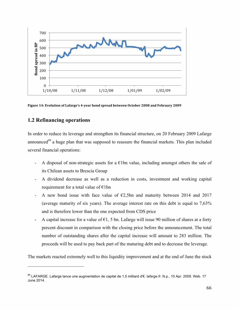
66
Figure 14: Evolution of Lafarge’s 4-‐year bond spread between October 2008 and February 2009
1.2 Refinancing operations
In order to reduce its leverage and strengthen its financial structure, on 20 February 2009 Lafarge
announced89 a huge plan that was supposed to reassure the financial markets. This plan included
several financial operations:
- A disposal of non-strategic assets for a €1bn value, including amongst others the sale of
its Chilean assets to Brescia Group
- A dividend decrease as well as a reduction in costs, investment and working capital
requirement for a total value of €1bn
- A new bond issue with face value of €2,5bn and maturity between 2014 and 2017
(average maturity of six years). The average interest rate on this debt is equal to 7,63%
and is therefore lower than the one expected from CDS price
- A capital increase for a value of €1, 5 bn. Lafarge will issue 90 million of shares at a forty
percent discount in comparison with the closing price before the announcement. The total
number of outstanding shares after the capital increase will amount to 283 million. The
proceeds will be used to pay back part of the maturing debt and to decrease the leverage.
The markets reacted extremely well to this liquidity improvement and at the end of June the stock
89 LAFARGE. Lafarge lance une augmentation de capital de 1,5 milliard d'€. lafarge.fr. N.p., 10 Apr. 2009. Web. 17 June 2014.
0
100
200
300
400
500
600
700
1/10/08 1/11/08 1/12/08 1/01/09 1/02/09
Bond spread in BP

67
price increased by around 30% in comparison with the beginning of year average, to 48,25€.
Similarly, the CDS spread decreased from 925bp to 300bp as the refinancing exposure of Lafarge
disappeared. The refinancing gap value is indeed equal to €400 million and represents only 1, 3%
of the firm value.
Figure 15 Evolution of Lafarge’s CDS spread and stock price between February 2009 and June 2009
This observation is the opposite of what classical structural models predicted. According to them,
the capital increase will lead to a dilution of the equity value and a transfer of value from the
shareholders to the debt holders due to the lower spread on the debt, hence a lower stock price.
The CreditGrades model therefore forecasted a decrease by 35% of the stock price by the end of
June 2009.
On the other hand, the refinancing gap model correctly predicted a stock increase. According to
the model, the price will rise to 49,66€, representing an increase of 20%. Moreover, this price is
close to the observed price of 48,25€. This stock increase is due to the transfer of the refinancing
gap value to the equity holders as the refinancing risk disappeared. This transfer of value more
than offset the diluting effect of the capital increase and the lower yield on the outstanding debt.
Similarly, the bond spread also reacted positively to the refinancing operations and went down to
300bp at the end of June, representing a decrease of 200bp. Once again, the classical structural
models failed to predict the exact spread and forecasted 107bp. This estimation is similar to the
one of the refinancing gap model (111bp). However, the refinancing gap model successfully
0
10
20
30
40
50
60 0 100 200 300 400 500 600 700 800 900
Stock price (inversed)
CDS spread (in BP)
CDS spread
Stock price

68
predicted the magnitude of the decrease. The spread indeed decreased by 200 bp in reality while
the refinancing gap model forecasted a decrease by 231bp.
Figure 16: Evolution of Lafarge’s 4-‐year bond spread between February 2009 and June 2009
1.3 Conclusion
The Refinancing gap model successfully predicts the initial and final stock price, hence the
magnitude of the change. It therefore provides an appealing explanation to the surprisingly
positive reaction of the stock price following the announcement of the refinancing operations.
Classical structural models are indeed not able to predict such reaction and forecast a decrease of
the stock price.
Although the refinancing gap model is not able to correctly predict the initial and final bond
spread, it offers a closer estimation than the classical structural models. Moreover, he
successfully forecasted the magnitude of change in the bond spread.
0
100
200
300
400
500
600
20/02/09 20/03/09 20/04/09 20/05/09 20/06/09
Bond spread in BP

69
Figure 17: Predictive power of Refinancing gap and classical structural models

70
Section 2: Pernod Ricard
Figure 18: Overview of Pernod Ricard’s case
2.1 Description and initial situation
Pernod Ricard is a French company that produces distilled beverages. The company is organized
in two entities, namely “beverages” and “distribution”. Pernod Ricard owns a portfolio of various
brands including Ricard, Havana Club, Mumm and Jacob’s Creek. Its products are distributed in
70 countries, the biggest markets being Europe and North America. Over the last decade, Pernod
Ricard has launched a strategy of "premiumisation" of its portfolio, aiming to become the global
leader in the premium beverage segment. As part of this strategy, on 31 March 2008 it
announced90 the acquisition of Vin & Sprit. Vin & Sprit is a Swedish producer and distributor of
alcoholic beverages that belonged to the Swedish government. The company is best known for its
“Absolut” brand of vodka. Absolut is the number one premium vodka worldwide and is the best
sold premium spirit brand in the United States. This acquisition allowed Pernod Ricard to add an
iconic vodka brand to its portfolio while becoming the co-leader in the global wine and spirit
industry and the sole leader in the premium segment.
Pernod Ricard offered a price of $5, 3 billion in exchange of 100% of the stock. Moreover, it took
on $0, 3 billion of debt in its own financial account for a total price of €5, 6 billion. The operation
was fully financed by debt and Pernod Ricard concluded a credit agreement with a pool of banks
90 PERNOD RICARD. Pernod Ricard acquiert Vin & Sprit et devient co-leader mondial de l’industrie des vins et spiritueux. Pernord-ricard.fr. N.p., 31 Mar. 2008. Thu. 18 June 2014.

71
for the total value of the deal. At the end of 2008 the total debt value amounted to €13, 5 billion
up from €6, 5 billion.
The acquisition led to a highly leveraged financial structure that ultimately triggered a rating
downgrade with negative outlook from the three main rating agencies. Pernod Ricard therefore
lost its Investment Grade rating and become a High Yield company. S&P justified this decision
by the too high debt per EBITDA ratio of the company following the acquisition and claimed that
in order to keep this rating unchanged in the future, Pernod Ricard would have to deleverage to
an adequate level of debt. Following these rating downgrades, the bondholder’s willingness to
hedge credit risk increased and the CDS spread was put under pressure, rising from 2% before the
acquisition to 7, 4% at the end of the year. Moreover, the company will have to refinance a
significant part of its debt during the next four years.
Figure 19: Pernod Ricard’s debt payment schedule
As the CDS spread has sharply increased over the last six month, the interest rate that Pernod
Ricard will need to pay on its new debt will be higher than the current one, possibly leading to a
liquidity problem. This situation will worsen the CDS spread even more.
Between the credit downgrade of October 2008 and April 2009, the stock price decreased by
around 30% from 57€ to 40€. Similarly, the CDS spread rose from 2% to 5, 92%.
-‐ -‐
1.500
3.300
200
8.500
-‐ 1.000 2.000 3.000 4.000 5.000 6.000 7.000 8.000 9.000
2009 2010 2011 2012 2013 2014
Maturing debt in € million

72
Figure 20 Evolution of Pernod Ricard’s CDS spread and stock price between October 2008 and April 2009
Classical structural models and financial analyst reports predicted a higher price at the beginning
of 2009. They set a target price of 46,44€, 15% higher than the market price. This difference in
price can be explained by the refinancing risk not taken into account by financial analysts. This
refinancing risk came from an expected interest rate on the future debt, which is 3, 28% higher
than on the outstanding debt. This premium must be considered a cost for the company.
According to the refinancing gap model, the value of this gap is equal to 10% of the value of the
firm and directly lowered the equity value. The refinancing model predicts a stock price of 40,
19€, which is in line with the observed market price.
Moreover, the refinancing gap model predicts a 5-year bond spread slightly higher than the one
of the classical structural models, 171 bp instead of 153bp. These forecasts are however 260bp to
280bp too low in comparison with the average bond spread over the period.
0 10 20 30 40 50 60 70 0
100 200 300 400 500 600 700 800 900
Stock price (inversed)
CDS spread
CDS
Stock
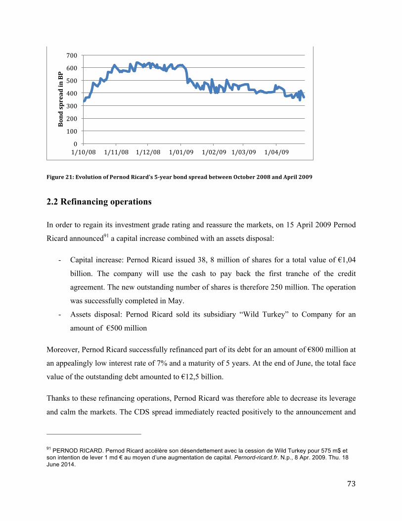
73
Figure 21: Evolution of Pernod Ricard’s 5-‐year bond spread between October 2008 and April 2009
2.2 Refinancing operations
In order to regain its investment grade rating and reassure the markets, on 15 April 2009 Pernod
Ricard announced91 a capital increase combined with an assets disposal:
- Capital increase: Pernod Ricard issued 38, 8 million of shares for a total value of €1,04
billion. The company will use the cash to pay back the first tranche of the credit
agreement. The new outstanding number of shares is therefore 250 million. The operation
was successfully completed in May.
- Assets disposal: Pernod Ricard sold its subsidiary “Wild Turkey” to Company for an
amount of €500 million
Moreover, Pernod Ricard successfully refinanced part of its debt for an amount of €800 million at
an appealingly low interest rate of 7% and a maturity of 5 years. At the end of June, the total face
value of the outstanding debt amounted to €12,5 billion.
Thanks to these refinancing operations, Pernod Ricard was therefore able to decrease its leverage
and calm the markets. The CDS spread immediately reacted positively to the announcement and
91 PERNOD RICARD. Pernod Ricard accélère son désendettement avec la cession de Wild Turkey pour 575 m$ et son intention de lever 1 md € au moyen d’une augmentation de capital. Pernord-ricard.fr. N.p., 8 Apr. 2009. Thu. 18 June 2014.
0
100
200
300
400
500
600
700
1/10/08 1/11/08 1/12/08 1/01/09 1/02/09 1/03/09 1/04/09
Bond spread in BP

74
fell to 3, 5% over the next month. This CDS spread was in line with the credit spread Pernod
Ricard paid on the outstanding debt, showing that the market did not fear the refinancing risk
anymore. The refinancing gap value was indeed divided by four following the increase in
liquidity and therefore amounted to only 2, 5% of the total firm value.
Similarly, the shareholders welcomed positively the capital increase and assets disposal and the
stock price rose to 42,62€ on average during the next three months following the announcement,
representing an increase of 6%.
Figure 22: Evolution of Pernod Ricard’s CDS spread and stock price between April 2009 and July 2009
As explained in chapter 2, classical structural models typically react negatively to a capital
increase announcement as the equity value is diluted amongst a higher number of shareholders.
The Pernod Ricard case was no exception and CreditGrades model predicted a decrease by 8, 5%
of the stock price.
According to the refinancing gap model on the other hand, the stock price is assumed to increase
by 5% up to 42,89€. This prediction is once again in line with the observed average price of 42,
62 and can be explained by the sharp decrease in the refinancing gap value. As mentioned in the
previous paragraph, the refinancing cost has indeed been divided by five following the
announcement and this decrease in the hidden debt has been transferred to the shareholders. The
refinancing gap model justifies the observed stock price increase by the higher transfer value to
the shareholders than the dilution effect due to the capital increase and the transfer from
shareholders to debt holders due to the lower credit risk of the firm.
36
38
40
42
44
46
48 0 50 100 150 200 250 300 350 400 450 500
15/04/09 15/05/09 15/06/09 15/07/09 Stock price (inversed)
CDS spread
CDS
Stock

75
Similarly, the 5-year bond spread reacted positively and decreased by 160bp to 267bp. Both
classical structural and refinancing gap models fail to predict this observation. Their estimations
are indeed 137bp too low (130bp instead of 267bp). In this case, the refinancing gap model is not
able to predict the magnitude of change (44bp instead of 120bp).
Figure 23: Evolution of Pernod Ricard’s 5-‐year bond spread between April 2009 and July 2009
2.3 Conclusion
The Refinancing gap model successfully predicts the initial and final stock price, hence the
magnitude of the change. On the other hand, classical structural models fail to forecast both the
initial price and the magnitude of change. According to them, the stock price is supposed to
decline due to the equity dilution following the capital increase.
Although both classical structural models and refinancing gap model fail to predict the initial and
final bond spread, the refinancing gap model forecast higher spread which shows the interest of
taking the refinancing exposure into account.
0 50 100 150 200 250 300 350 400 450
Bond spread in BP

76
Figure 24: Predictive power of Refinancing gap and classical structural models
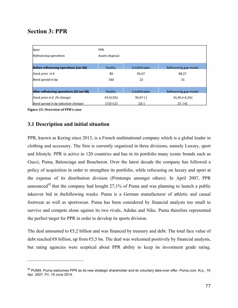
77
Section 3: PPR
Figure 25: Overview of PPR’s case
3.1 Description and initial situation
PPR, known as Kering since 2013, is a French multinational company which is a global leader in
clothing and accessory. The firm is currently organized in three divisions, namely Luxury, sport
and lifestyle. PPR is active in 120 countries and has in its portfolio many iconic brands such as
Gucci, Puma, Balenciaga and Boucheron. Over the latest decade the company has followed a
policy of acquisition in order to strengthen its portfolio, while refocusing on luxury and sport at
the expense of its distribution division (Printemps amongst others). In April 2007, PPR
announced92 that the company had bought 27,1% of Puma and was planning to launch a public
takeover bid in thefollowing weeks. Puma is a German manufacturer of athletic and casual
footwear as well as sportswear. Puma has been considered by financial analysts too small to
survive and compete alone against its two rivals, Adidas and Nike. Puma therefore represented
the perfect target for PPR in order to develop its sports division.
The deal amounted to €5,2 billion and was financed by treasury and debt. The total face value of
debt reached €8 billion, up from €5,5 bn. The deal was welcomed positively by financial analysts,
but rating agencies were sceptical about PPR ability to keep its investment grade rating.
92 PUMA. Puma welcomes PPR as its new strategic shareholder and its voluntary take-over offer. Puma.com. N.p., 10 Apr. 2007. Fri. 19 June 2014.

78
According to S&P, PPR will not be able to continue its acquisition policy and conserve its
investment grade rating at the same time. S&P therefore advised PPR to dispose some of its
assets in order to come back to a more reasonable leverage ratio. Moreover, the financial
structure of the company is such that it will have to refinance more than half of its debt over the
next two years. Given the uncertainty about its future rating as well as the negative prospects for
the luxury industry due to the financial crisis, the company will have to pay a premium of around
1,5% in comparison with its current average interest rate.
Figure 26: PPR’s debt payment schedule
Financial analysts estimated the fair price of the company stock at the beginning of 2008 to be
comprised between 95 and 105€. However, the averaged observed price between January 1st and
January 23rd was equal to 89€, about 10% lower than the target price. On the other hand, the
refinancing gap model computed a target price of 88,27€ per share, which is closer to the actual
price. The model has achieved this accuracy by taking into account the refinancing risk, the
refinancing gap value representing 7% of the firm value for an amount of €1,25 billion.
3420
959
183
920
1772
836
0 €
500 €
1.000 €
1.500 €
2.000 €
2.500 €
3.000 €
3.500 €
4.000 €
2008 2009 2010 2011 2012 2013
Maturing debt in € million

79
Figure 27: Evolution of PPR’s CDS spread and stock price between November 2007 and January 2008
Similarly, the average 3-year bond spread over the three first weeks of January 2009 was equal to
160bp. This actual spread failed to be predicted by both the classical structural models (22bp) and
the refinancing gap (31bp). However, the forecast of the refinancing gap model is 30% higher in
absolute terms.
Figure 28: Evolution of PPR’s 3-‐year bond spread between December 2007 and January 2008
0
20
40
60
80
100
120
140
160 0 20 40 60 80 100 120 140 160 180
1/11/07 1/12/07 1/01/08
Bond spread (inversed)
CDS spread (in BP)
CDS spread
Stock price
130 135 140 145 150 155 160 165 170 175 180
14/12/07
16/12/07
18/12/07
20/12/07
22/12/07
24/12/07
26/12/07
28/12/07
30/12/07
1/01/08
3/01/08
5/01/08
7/01/08
9/01/08
11/01/08
13/01/08
15/01/08
17/01/08
19/01/08
21/01/08
23/01/08
Bond spraed in BP

80
3.2 Refinancing operations
In order to comply with rating recommendations by the agencies and increase its liquidity, PPR
announced93 on January 24th that it would sell its subsidiary “Yves Saint-Laurent Beauté” to
L’Oreal for a total amount of €1,2 billion. YSL Beauté commercializes under license fragrance
brands such as Cacharel, Diesel or YSL and also owns the cosmetics brand “Roger & Gallet”.
The brand struggled to reach profitability when it operated under the PPR management. PPR
executives therefore claimed that a company such as l’Oréal would be in a better position to
exploit YSL Beauté ‘s full potential thanks to its expertise in fragrance and cosmetics.
Surprisingly, the stock price reacted extremely well and increased by 12% on the day of
announcement and stabilized around 93€ over the next two weeks, representing a 4, 5% rise.
Figure 29: Evolution of PPR’s CDS spread and stock price between January 2008 and February 2008
This surprised financial analysts because the disposal price was in line with their estimation and
the stock price was therefore supposed not to vary following the news (the loss of future cash
flow was indeed perfectly compensated by the increase in cash following the disposal, such as the
firm value and the equity value did not change). This stock behaviour can be explained by the
improved liquidity of PPR following the operation. Thanks to the disposal proceeds, the company
will be able to refinance its maturing debt without having to go on the debt market. Therefore, the
93 LE FIGARO. L'Oréal s'offre Yves Saint Laurent Beauté . Lefigaro.fr. N.p., 24 Jan. 2009. Fri. 19 June 2014.
75
80
85
90
95
100 0 20 40 60 80 100 120 140 160 180
10/01/08
12/01/08
14/01/08
16/01/08
18/01/08
20/01/08
22/01/08
24/01/08
26/01/08
28/01/08
30/01/08
1/02/08
3/02/08
5/02/08
Stock price (inversed)
Credit spread
CDS
Stock

81
refinancing gap lost half of its value that was directly transferred to the shareholders, hence an
increase of the stock price. According to the refinancing gap model, the target stock price
following the disposal was equal to 91,96€. This price was really close to the observed one and
represents an increase of 4,2% comparing to the target price before the operation.
The YSL Beauté disposal was therefore accretive for the shareholders. However, the market price
quickly plummeted due to the bad luxury industry outlook and was therefore not able to sustain
the target price.
Finally, while both models predicted a spread around 25bp (which represents a 25% decline in
the case of the refinancing gap model and a stabilisation for classical structural ones), the actual
bond spread slightly increased to 172bp.
Figure 30: Evolution of PPR’s 3-‐year bond spread between January 2008 and February 2008
3.3 Conclusion
Although the classical structural models predict that an asset disposal at a fair price does not
affect the stock price, PPR’s reacted positively to the disposal. The refinancing gap model is able
to explain this increase in stock price. Moreover, it offers closer to reality prices than classical
structural models.
160
165
170
175
180
185
Bond spraed in BP

82
Similarly, the refinancing gap model forecasts a higher bond spread than the classical structural
models, both initially and after the refinancing operations. However, these spreads are still far
from the reality.
Figure 31: Predictive power of Refinancing gap and classical structural models

83
Section 4: TUI AG
Figure 32: Overview of TUI AG’s case
4.1 Description and initial situation
TUI AG is a German multinational travel and tourism company. It owns travel agencies, airlines,
cruise ships and retail stores. TUI AG is one of the world’s largest tourist firms and is divided in
four subsidiaries: TUI Travel, Hapag Lloyd, Hotels and Cruises. TUI AG significantly suffered
from the financial crisis starting in 2008 and the general drop in leisure expenses that followed.
Moreover, the company faced a severe liquidity issue at the end of 2008. It would have to
refinance more than half of its debt over the next three years. However, its cash flow generation
is not high enough to face these financial obligations and its reserve of cash, although appealing
on paper, is nearly entirely in the form of a loan to TUI travel and is restricted until 2011. Out of
the € 1,7 billion cash reserve, only €300 million was directly available to TUI AG. This is very
low given TUI AG corporate needs and working capital was swinging. Moreover, the leverage
ratio was also considerable and the total face value of debt amounted to €5,3 billion. This
liquidity issues triggered a rating downgrade at the beginning of December 2008, from BB- to B+
according to S&P. This downgrade directly impacted the CDS market. Investors indeed grew
increasingly worried about TUI AG’s ability to meet its next financial obligations and the 5-year
CDS soared from 8, 68% before the announcement to more than 12% two months later. This led
to a potential credit premium of around 12% if TUI needed to refinance its debt at this moment,
in comparison with the average interest rate it was currently paying on its outstanding debt. This

84
situation worsened even more the liquidity trap in which TUI AG was. Altogether it looked like a
vicious circle for the company.
Figure 33: TUI AG's debt payment schedule
According to the refinancing gap model, the value of this liquidity trap amounted to 30% of the
total assets value, for a value of more than €2,5 billion. This refinancing gap could therefore have
a great negative impact on the stock price, which was verified by the historical data. Over the last
six months (August 2008 – January 2009), the stock price tumbled by around 66% and the price
in the beginning of February fluctuated around 5€
This observation is close to the computation of the refinancing gap model. The model indeed
predicts a target price around 6,5€ when refinancing risk is taken into account. On the other hand,
classical structural models predicted a target price around 14€ which is more than two times the
observed price and therefore appears unrealistic.
800
1.150
800
1.800
800
-‐ 200 400 600 800
1.000 1.200 1.400 1.600 1.800 2.000
800 1.150 800 1.800 800
Maturing debt in € million

85
Figure 34: Evolution of TUI AG’s CDS spread and stock price between January 2008 and February 2008
The 3-year bond spread reacted sharply to this distressed situation and was be multiplied by four
to 1972bp. Although both structural and refinancing gap models failed to predict this level of
spread, the refinancing gap model forecasted a spread 30% higher in absolute terms than the
classical structural models (402bp instead of 315bp).
Figure 35: Evolution of TUI AG’s 3-‐year bond spread between August 2008 and February 2009
4.2 Refinancing operations
In order to solve this liquidity issue, on October 12, 2008 UI AG announced its willingness to sell
its shipping division, Hapag-Lloyd. TUI AG was indeed willing to refocus on the tourism
business and the cash inflow from the operation would solve a significant part of the liquidity
issue. Rumours claimed that TUI AG had entered into negotiations with the German consortium
Albert Ballin KG and that they had agreed on the following terms:
0 2 4 6 8 10 12 14 16 0
500
1000
1500
2000
2500
Stock price
CDS spread (in BP)
CDS spread
Stock price
0
500
1000
1500
2000
2500
1/08/08 1/09/08 1/10/08 1/11/08 1/12/08 1/01/09 1/02/09
Bond spread in BP

86
- Hapag-Lloyd total value is estimated at €4,45 billion out of which €1,3 billion represents
the net debt
- Albert Ballin KG will pay €2,7 billion in cash in exchange of 2/3 of the shares
- TUI AG will conserve 1/3 of the shares in the new entity.
However, on February 27, TUI AG announced that it had come to an agreement with Albert
Ballin KG, but under slightly different terms than the ones presented in the press the weeks
before: TUI AG indeed will keep 43,33% of the shares in the new entity. The net proceed
received by TUI AG will amount to €1,6 billion. TUI AG’s management did not announce at that
time what they were planning to do with the cash. Although financial analysts would like the firm
to pay back its debt in order to deleverage, a clause in case of assets disposal included in a bond
issue contract stated that the disposal proceeds must be reinvested at last one year later at the
latest in new assets. The remaining cash must then be used to pay back a given debt in priority.
The stock price reacted extremely positively to the announcement and increased by 53% over the
next two months to 7,68€. This observation is in contradiction with classical structural model
prediction. As the disposal price was in line with the market expectation, these models indeed
assume that the decrease in future cash flow is fully compensated by the inflow of cash, such as
the firm value and hence the equity values remain the same. Therefore, the stock price should not
react to the disposal announcement.
The refinancing gap model predicts an increase by 40% of the stock price (to 9, 55€), which is in
line with the observation. This sharp increase in price can be explained by the reduction of the
liquidity and refinancing risks. These risks decreased and so did the value of the refinancing gap.
The latter was divided by six thanks to the disposal and only amounted to 5% of the total firm
value. This decrease in value was transferred to the shareholders, hence the stock price increased.

87
Figure 36: Evolution of TUI AG’s CDS spread and stock price between February 2008 and April 2008
Finally, the 3-year bond spread increased by nearly 200 to 2148bp over the next two months.
This observation is in contradiction with both structural and refinancing gap models that
predicted either a spread decline (in the case of the refinancing gap model, by 150bp to 337bp) or
a stabilisation (classical structural models, to 315bp).
Figure 37: Evolution of TUI AG’s 3-‐year bond spread between February 2009 and April 2009
0 1 2 3 4 5 6 7 8 9 0
500
1000
1500
2000
2500
27/02/09 27/03/09 27/04/09
Stock price
CDS spread (in BP)
CDS spread
Stock price
0
500
1000
1500
2000
2500
3000
Bond spread in BP

88
4.3 Conclusion
The sharp increase in TUI AG’s stock price following Hapag-Lloyd is correctly predicted by the
refinancing gap model. On the other hand, classical structural models assume that no variation is
anticipated. Moreover, the refinancing gap model forecasts stock prices that are closer from
reality, both before and after the refinancing operations.
Regarding the bond market, the Refinancing gap model predicts a spread which is 50% higher in
absolute terms than the one predicted by classical structural models, yet far from the observed
one.
Figure 38: Predictive power of Refinancing gap and classical structural models

89
Section 5: KPN
Figure 39: Overview of KPN’s case
5.1 Description and initial situation
KPN is a Dutch landline and mobile telecommunications company. The firm is organized around
two main divisions: the fixed line division, which counts around six million customers in the
Netherlands and the mobile division, which is active in the Netherlands, Germany, Belgium,
France and Spain and has 33 million subscribers. Its main markets are the Netherlands and
Germany. Although KPN cash generation appears attractive with an EBIDTA of €4 billion in
2012, the company suffered from a high level of debt, contracted to finance past acquisitions. The
face value on the outstanding debt had amounted to more than €14 billion at the end of 2012 and
its debt/EBITDA ratio was close to three. Moreover, KPN was facing both a sharp competitive
environment triggering a price war in its two core markets and a poor outlook for the
telecommunication business in general.
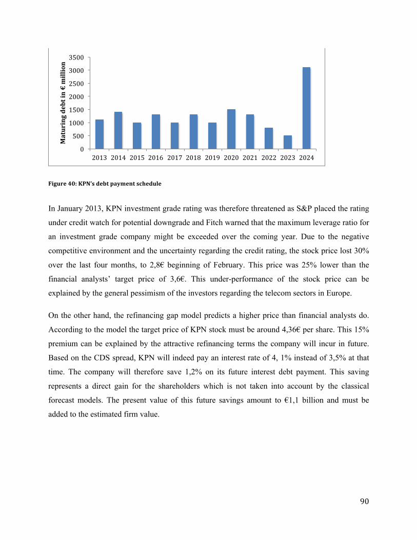
90
Figure 40: KPN’s debt payment schedule
In January 2013, KPN investment grade rating was therefore threatened as S&P placed the rating
under credit watch for potential downgrade and Fitch warned that the maximum leverage ratio for
an investment grade company might be exceeded over the coming year. Due to the negative
competitive environment and the uncertainty regarding the credit rating, the stock price lost 30%
over the last four months, to 2,8€ beginning of February. This price was 25% lower than the
financial analysts’ target price of 3,6€. This under-performance of the stock price can be
explained by the general pessimism of the investors regarding the telecom sectors in Europe.
On the other hand, the refinancing gap model predicts a higher price than financial analysts do.
According to the model the target price of KPN stock must be around 4,36€ per share. This 15%
premium can be explained by the attractive refinancing terms the company will incur in future.
Based on the CDS spread, KPN will indeed pay an interest rate of 4, 1% instead of 3,5% at that
time. The company will therefore save 1,2% on its future interest debt payment. This saving
represents a direct gain for the shareholders which is not taken into account by the classical
forecast models. The present value of this future savings amount to €1,1 billion and must be
added to the estimated firm value.
0
500
1000
1500
2000
2500
3000
3500
2013 2014 2015 2016 2017 2018 2019 2020 2021 2022 2023 2024
Maturing debt in € million

91
Figure 41: Evolution of KPN’s spread and stock price between October 2012 and February 2013
Moreover, the 10-year bond spread increased by 30bp to around 202bp on average at the end of
January 2013. This is 25bp lower than the refinancing gap estimation of 227bp. However, the
classical structural models predicted a spread of 212bp which is more in line whith the
observation. In the case of a company with a negative refinancing exposure, the refinancing gap
model has therefore the tendency to overestimate the spread and offers less accuracy than
classical structural models.
Figure 42: Evolution of KPN 10-‐year bond spread between February 2009 and April 2009
0
0,5
1
1,5
2
2,5
3
3,5
4 0
50
100
150
200
250
5/10/12 5/11/12 5/12/12 5/01/13 5/02/13
Stock price
CDS spread (in BP)
CDS
Stock
0
50
100
150
200
250
5/10/12 5/11/12 5/12/12 5/01/13 5/02/13
Bond spread in bp

92
5.2 Refinancing operations
On February 5th 2013, KPN announced94 that it intended to raise €4 billion of capital through a
right issue. The company justified this operation by its willingness to improve and deleverage its
financial structure in order to maintain its investment grade rating. The operation will consist in
the creation of 2, 8 billion new shares to be sold at a 35% discount for a new total of 4, 2 billion
outstanding shares.
As expected, the financial markets reacted negatively to the news and the stock price lost 38% of
its value over the next month. This stock behaviour is explained by the important dilution of the
equity value due to the capital increase, the number of outstanding shares being multiplied by
three. However, the classical models failed to predict the exact magnitude of this decrease. The
predicted range is indeed comprised between 25% and 30% depending on the model. The
refinancing gap model on the contrary, successfully forecasted a 36% decrease, close to the
actual one.
The accuracy of the refinancing gap model is explained by the change in future refinancing
needs. As highlighted before, KPN will be able to refinance its future debt at a lower cost than
the outstanding one. This situation represents a saving for the shareholders that directly increases
the firm value, hence the equity value. By raising a considerable amount of capital, KPN
improves its liquidity and therefore reduces the amount of debt that will need to be rolled over.
As a consequence, KPN’s exposure to the future interest rates decreases and the company will
not benefit to the same extent from the appealing future refinancing terms. The savings for the
shareholders will therefore drop and so will the equity value. At the end, the decline in stock
price is explained by the combined effects of dilution and lower exposure to positive refinancing
terms.
It is however important to note that both classical and refinancing gap models predict a target
price which is comprised between 2,6€ and 2,8€ and is therefore far from the observed one.
94 THE NEW YORK TIMES. KPN to Raise 4 Billion Euros to Fend Off Rivals. nytimes.com. N.p., 5 Feb. 2013. Sun. 20 June 2014.

93
Financial analysts explained this situation by the overreaction of the investors to the increased
competition and the negative outlook of the telecom market in Europe. They however remain
confident that the stock prise will tend to its target price once the investors are reassured.
Figure 43: Evolution of KPN’s spread and stock price between February 2013 and March 2013
The 10-year spread first reacted negatively to the capital increase announcement and increased by
20bp. However, the spread went down to its initial level after three weeks, around 190bp. Both
structural and Refinancing gap model predicts the same target spread of 83bp which is more than
100bp too low.
Figure 44: Evolution of KPN 10-‐year bond spread between February 2009 and April 2009
0
0,5
1
1,5
2
2,5 150
155
160
165
170
175
6/02/13
8/02/13
10/02/13
12/02/13
14/02/13
16/02/13
18/02/13
20/02/13
22/02/13
24/02/13
26/02/13
28/02/13
2/03/13
4/03/13
Stock price
CDS spread (in BP)
CDS
Stock
170 175 180 185 190 195 200 205 210
Bond spread in bp

94
5.3 Conclusion
Although both classical structural and Refinancing gap models fail to predict the stock price
before and after the refinancing operations, the refinancing gap model correctly anticipates the
magnitude of the price decrease.
Moreover, in this case of a company with a negative refinancing exposure, the Refinancing gap
model has the tendency to over predict the observed spread and offers less accurate results than
the classical structural models.
Figure 45: Predictive power of Refinancing gap and classical structural models

95
Section 6: Summary
This chapter outlined the practical application of the Refinancing gap model to five companies
with an exposure to the refinancing risk. It appears that the refinancing gap model is better
equipped to predict the stock price of a distressed company before and after a refinancing
operation than the classical structural models. This observation therefore proves the relevance of
the refinancing approach when dealing with distressed companies. However, predictive power of
the refinancing gap model seems less appealing when dealing with companies facing a negative
refinancing exposure, although it correctly predicts the magnitude of change of the stock price.
Finally, the refinancing gap model offers higher bond spreads than those predicted by classical
structural models. The refinancing gap model therefore improves the accuracy of these structural
models in the case of company with a positive refinancing exposure. However, the forecasted
spreads are still far from reality.
The refinancing gap model therefore appears to be a useful tool for equity analysts and can serve
as a basis for further research in credit modelling.

96
Conclusion The focus of this dissertation was to study the impact of the refinancing risk on the value of a
firm and how the latter reacts to refinancing operations. It was intuitively assumed that, by
forcing companies to pay a higher future interest rate, refinancing risk influences negatively the
probability of default of a firm, hence its value. On the other hand, refinancing operations were
expected to improve the liquidity of the company and consequently reduce its refinancing
exposure. In order to be in a position to answer this question thoroughly and confirm or infirm
these intuitions, this dissertation first analysed the existing literature over the default modelling
and its influence on the firm value before presenting a model that deals with the refinancing risk.
It appears from the literature review that none of the current models takes the refinancing risk
into account when modelling the probability of default of a firm and indirectly its value. As a
matter of fact classical structural models assume that a company defaults as soon as its firm value
falls below a given threshold. Although this threshold depends on the specificities of the model,
structural models rely only on economic distress to trigger off the default of a firm. By doing so,
they fail to take another kind of distress into account, that is to say the financial distress.
Financial distress occurs when the company faces difficulties to honour its financial obligations
and is therefore considered a cash flows or liquidity issue. Refinancing risk is therefore a subset
of this liquidity risk as uncertainty regarding the refinancing terms directly impacts the liquidity
of a firm. As a consequence, classical structural models either assume that the company will be
able to refinance its total debt under the current terms in the future or that the company will stop
existing at the maturity of the outstanding debt. These assumptions are obviously not verified in
reality and require the development of a new model to deal with the refinancing risk.
This new model, called the “Refinancing gap model”, is based on a cash flow approach of the
refinancing risk. In fact the company has to finance its future activities, yielding a known cash
flow, by borrowing at an unknown rate. This situation is similar to a swap position for the
company, in which it receives fixed cash flows from operating activities and has to pay an
interest rate on its future debt that will only be determined when the debt is rolled over. This
swap should be considered an off balance sheet item and is similar to a hidden debt in the case of

97
a distressed company whose expected refinancing terms have worsened. The value of this swap
represents the exposure of the firm to the refinancing risk. As this exposure is considered a
hidden debt, it directly influences the value of both equity and debt. On one hand, this hidden
debt increases the total leverage of the firm, hence the credit risk of the debt. As a consequence,
the credit spread on the debt will also increase, which will negatively impact the value of the
debt. On the other hand, the hidden debt represents the part of the value of the firm which is
locked due to the refinancing exposure and is therefore currently not available for the
shareholders, resulting in a lower value of the equity. As part of the value of the firm is therefore
locked and not attributed to either the shareholders or the debt holders, the actual value of the
firm, equal to the sum of the equity and he debt value, is lower than the one of a similar firm
without exposure to the refinancing risk.
A distressed company with an exposure to the refinancing risk has various options to reduce this
exposure. These operations (i.e. capital increase, assets disposal, etc) will have a positive impact
on the liquidity of the firm, hence reducing the exposure and the value of the hidden debt. In turn
a reduction in the hidden debt will positively affect the equity and debt value, hence the actual
firm value. On one hand, the reduction in the hidden debt decreases the leverage of the firm and
consequently its credit risk. On the other hand, the refinancing operation will unlock part of the
firm value, which will directly be transferred to the equity.
In theory the refinancing gap model is therefore able to explain how the refinancing exposure
affects a firm value and how the latter reacts to refinancing operations. The model was finally
applied on existing companies to test whether it predicts accurately the equity and debt value of
distressed companies in real terms. It turned out that the refinancing gap model is efficient to
predict the stock price of distressed companies and improves the accuracy of classical structural
models when forecasting the bond spread.
Indeed the refinancing gap model has successfully predicted the stock prices of the four studied
companies before and after the refinancing operations. Furthermore, it outperformed significantly
the classical structural models used as a benchmark. Moreover, the model successfully predicts
the magnitude of the stock price variation when the firm announces its refinancing operations,

98
which is impossible by means of the classical structural models. It is clear that these models
provide forecasts that are usually contrary to the stock market reaction. Considering that the
refinancing exposure locks part of the value of the firm to the detriment of the shareholders
therefore appears to be a relevant approach. Moreover this is in line with the stock market
reaction to such exposure.
On the other hand, the refinancing gap model systematically predicts bond spreads that are higher
than those of classical structural models, hence improving the accuracy of these models.
Moreover, the biggest improvements appear for companies that face a considerable refinancing
exposure. As a consequence, it proofs that the refinancing risk significantly impacts the bond
spread of a distressed company and justifies partly the “underprediction” of the classical
structural models. However, the Refinancing gap model still fails to accurately predict the real
bond spread and only provides a closer estimation. By considering the refinancing risk in addition
to the economic distress, the refinancing gap model therefore takes into account a wider range of
financial triggers. However, the refinancing gap model does not consider the liquidity issue in its
broad sense. This limitation might explain the remaining difference between modelled and
observed spreads
Following these conclusions about the refinancing gap model as well as its limitations, four
improvements to this model can be proposed as future research directions.
Firstly, the last chapter of this dissertation applied the refinancing gap model on five different
distressed companies. This sample is too small to draw any conclusion regarding the accuracy of
the model from a statistical point of view. One could therefore decide to apply the model on a
statistically representative sample of companies in order to confirm or infirm the predictive
power of the model. This quantitative study would only require to process the financial data
available and apply the framework presented in chapter 2, without having to master the whole
history of each company as required by this dissertation.
Secondly, the refinancing gap model uses the relevant CDS spread to predict the future cost of
refinancing. However, few companies have a CDS quoted on their outstanding debt and an even

99
smaller proportion amongst them has a CDS which is sufficiently liquid. The approach proposed
in the dissertation therefore limits the range of company on which the Refinancing gap model can
be applied. To overcome this limitation, one could replicate the results presented in this
dissertation using other proxies such as the CDS spread estimated by Bloomberg for companies
without traded CDS.
Thirdly, the refinancing gap model allows to improve the classical structural models by taking
into account the refinancing risk. However, these models still fail to include liquidity in general
as a default trigger. This observation therefore opens a wide area of research to ultimately
propose a comprehensive model including all the elements influencing the credit risk of a firm.
Finally, this dissertation used two structural models to apply the refinancing gap model. These
models, the Merton and the CreditGrades model, were chosen for reasons of easiness of use and
the presence of the required parameters needed to use them. In the context of this dissertation, it
was indeed impossible to use computing-intensive models or ones which require the access to
advanced financial data. However, these two models are not the most performing ones in the
structural models category. One could therefore use the approach developed in this dissertation
and extend it to more advanced structural models. This should, in principle, improve the credit
spread predictive power of the current refinancing gap model.

100
Bibliography
• ALTMAN, Edward I. Financial ratios, discriminant analysis and the prediction of corporate bankruptcy. The journal of finance 23.4 (1968).
• ANDERSON, Ronald W., SUNDARESAN, Suresh, et TYCHON, Pierre. Strategic analysis of contingent claims. European Economic Review, 1996, vol. 40, no 3, p. 871-881.
• ARORA, Navneet, Jeffrey R. Bohn, and Fanlin Zhu. Reduced form vs. structural models of credit risk: A case study of three models. Journal of Investment Management 3.4 (2005).
• BANK FOR INTERNATIONAL SETTLEMENT. Long-term Rating Scales Comparison.
www.bis.org. n.d. 24 Mai 2014.
• BENITO, Enrique and Flavan, Silviu. A comparison of credit risk model, Carlos III University in Madrid, March 2005
• BLACK, Fischer and COX, John C. Valuing corporate securities: Some effects of bond indenture provisions. The Journal of Finance, 1976, vol. 31, no 2, p. 351-367.
• BLANCO, Roberto, BRENNAN, Simon, et MARSH, Ian W. An empirical analysis of the dynamic relation between investment-‐‑grade bonds and credit default swaps. The Journal of Finance, 2005, vol. 60, no 5.
• BRIYS, Eric and DE VARENNE, François. Valuing risky fixed rate debt: An extension.
Journal of Financial and Quantitative Analysis, 1997, vol. 32, no 02, p. 239-248.
• COUDERT, Virginie et GEX, Mathieu. Credit default swap and bond markets: which leads the other. Financial Stability Review, Banque de France, 2010, vol. 14, no 2010.
• CREDIT SUISSE, Leveraged Finance Outlook and 2013 Annual Review, 2013
• DARRELL, Duffie and SCHAEFER, Stephen, Credit Risk: Pricing, Measurement, and Management, Princeton, Princeton University Press, 2003.
• DAVYDENKO, Sergei A. When do firms default? A study of the default boundary. A Study of the Default Boundary (November 2012). EFA Moscow Meetings Paper. 2012,
• DE WIT, Jan. Exploring the CDS-bond basis. National Bank of Belgium, 2006.
• ELIZALDE, Abel. Credit risk models II: Credit risk models II: Structural models. 2005.

101
• EOM, Young Ho, HELWEGE, Jean, et HUANG, Jing-zhi. Structural models of corporate
bond pricing: An empirical analysis. Review of Financial studies, 2004, vol. 17, no 2, p. 499-544.
• EXANE, Capital Structure Optimization : CDS and share price, ALRG model and country risk, 2013.
• EXANE, The Asset Liability Refinancing Gap model : Valuation and Arbitrage of
indebted companies, January 2009
• FELIX, Jean-Paul. Notes de cours : Marchés financiers en temps continu et modélisation de taux. Université de Picardie, 2010.
• FINGER, Christopher, FINKELSTEIN, Vladimir, LARDY, Jean-Pierre, et al. CreditGrades technical document. RiskMetrics Group, 2002.
• GESKE, Robert. The valuation of corporate liabilities as compound options. Journal of
Financial and Quantitative Analysis, 1977, vol. 12, no 04
• HE, Zhiguo, and WEI Xiong. Rollover risk and credit risk. The Journal of Finance 67.2 (2012)
• Hu, H. and Lawrence, L. (2000). Estimating Recovery Rates, JPMorgan document
• HUANG, Jing-zhi et ZHOU, Hao. Specification analysis of structural credit risk models. In : AFA 2009 San Francisco Meetings Paper. 2008
• HULL, John C., PREDESCU, Mirela, et WHITE, Alan. Bond prices, default probabilities and risk premiums. Default Probabilities and Risk Premiums (March 9, 2005), 2005.
• HULL, John, PREDESCU, Mirela, et WHITE, Alan. The relationship between credit default swap spreads, bond yields, and credit rating announcements. Journal of Banking & Finance, 2004, vol. 28, no 11,
• Hull, John. Options, futures and other derivatives. Pearson education, 2012. 2nd ed.
• JARETZKE, Dominik. CDS Model and Market Spreads Amid the Financial Crisis. Maastricht University. 2010
• JARROW, Robert A. et PROTTER, Philip. Structural vs reduced form models: A new
information based perspective. Journal of Investment Management, 2004, vol. 2, no 2.
• JONES, E. Philip, MASON, Scott P., et ROSENFELD, Eric. Contingent claims analysis of corporate capital structures: An empirical investigation. The Journal of Finance, 1984, vol. 39, no 3, p. 611-625.

102
Journal of Investment Management 2.2 (2004).
• LAFARGE. Lafarge Acquiert Orascom Cement, Le Leader Cimentier Du Moyen-Orient Et Du Bassin Méditerranéen. www.lafarge.fr. N.p., 10 Dec. 2007. Web. 17 June 2014.
• LAFARGE. Lafarge lance une augmentation de capital de 1,5 milliard d'€. lafarge.fr. N.p., 10 Apr. 2009. Web. 17 June 2014.
• LE FIGARO. L'Oréal s'offre Yves Saint Laurent Beauté . Lefigaro.fr. N.p., 24 Jan. 2009. Fri. 19 June 2014.
• LELAND, Hayne E. "Predictions of default probabilities in structural models of debt." The credit market handbook: Advanced modeling issues (H. Gifford Fong, Editor) (2006),
• LELAND, Hayne E. et TOFT, Klaus Bjerre. Optimal capital structure, endogenous bankruptcy, and the term structure of credit spreads. The Journal of Finance, 1996, vol. 51, no 3, p. 987-1019.
• LONGSTAFF, Francis A. et SCHWARTZ, Eduardo S. A simple approach to valuing risky fixed and floating rate debt. The Journal of Finance, 1995, vol. 50, no 3, p. 789-819.
• MERTON, Robert C. "On the pricing of corporate debt: The risk structure of interest rates." The Journal of Finance 29.2 (1974).
• MOODY’S INVESTORS SERVICE. " Corporate Default and Recovery Rates, 1920-2010." (2011)
• MOODY’S INVESTORS SERVICE. "Rating methodology : Global shipping industry."
(2009)
• PERNOD RICARD. Pernod Ricard accélère son désendettement avec la cession de Wild Turkey pour 575 m$ et son intention de lever 1 md € au moyen d’une augmentation de capital. Pernord-ricard.fr. N.p., 8 Apr. 2009. Thu. 18 June 2014.
• PERNOD RICARD. Pernod Ricard acquiert Vin & Sprit et devient co-leader mondial de l’industrie des vins et spiritueux. Pernord-ricard.fr. N.p., 31 Mar. 2008. Thu. 18 June 2014.
• PUMA. Puma welcomes PPR as its new strategic shareholder and its voluntary take-over offer. Puma.com. N.p., 10 Apr. 2007. Fri. 19 June 2014.
• STANDARD & POOR’S, “Credit Trends: Gaping Refunding Pipeline In Europe Intensifies Financial Challenges“, 2010

103
• STEPHANOU, Constantinos, and MENDOZA, Juan Carlos. "Credit risk measurement under Basel II: an overview and implementation issues for developing countries." World Bank Policy Research Working Paper 3556 (2005).
• SUNDARESAN, Suresh. "A Review of Merton’s Model of the Firm’s Capital Structure with Its Wide Applications." Annu. Rev. Financ. Econ. 5.1 (2013).
• THE NEW YORK TIMES. KPN to Raise 4 Billion Euros to Fend Off Rivals. nytimes.com. N.p., 5 Feb. 2013. Sun. 20 June 2014.
• VAN BEEM, J. " Credit risk modeling and CDS valuation :An analysis of structural models." University of Twente (2010). p.22.
• WANG, Yu. "Structural Credit Risk Modeling: Merton and Beyond." Risk Management 16 (2009). p.30.
• ZHOU, Chunsheng. A jump-diffusion approach to modeling credit risk and valuing
defaultable securities, 1997.
Financial reports and analysis
Lafarge
• Lafarge, Annual Report 2007, 2007
• Lafarge, Annual Report 2008, 2008
• Exane Derivatives, Lafarge special report, 3 March 2009
• Deutsche Bank, First quarter results review,7 May 2009
Pernod Ricard
• Societe Generale Cross Asset Research, Pernod Ricard : Focus on credit metrics vs shareholder interests, 19 November 2009
• ING, Pernod Ricard :Premiumisation, if well executed, will continue, 15 January 2009
• Credit Suisse, Pernod Ricard: V&S Acquisition – Short Equity / Long Credit, 10 April 2008
• Societe Generale Cross Asset Research, PERNOD RICARD :Slightly too optimistic, weren’t they?, 13 February 2009

104
• Societe Generale Cross Asset Research, PERNOD RICARD : Able to hold a drink, 31 July 2008
• Merril Lynch, Low appetite for risk dilutes investment case, 19 September 2008
• Morgan Stanly, Pernod Ricard : Good start but growth drivers are weakening, 30 October 2008
• Deutsche Bank, Pernod Ricard, 30 0ctober 2008
• Merril Lynch, Pernod Ricard : Spirits industry sales appear resilient – are they?, 31 October 2008
• Moody’s Investors Service, Credit Opinion: Pernod Ricard S.A., 31 July 2008
• Moody’s Investors Service, Credit Opinion: Pernod Ricard S.A., 25 May 2009
• Moody’s Investors Service, Credit Opinion: Pernod Ricard S.A., 14 January 2008
• Moody’s Investors Service, Pernod Ricard : corporate profile, February 2009
• Pernod Ricard, Annual Report 2006, 2006
• Pernod Ricard, Annual Report 2007, 2007
• Pernod Ricard, Annual Report 2008, 2008
• Pernod Ricard, Acquisition of Vin & Sprit, 31 March 2008
• Morgan Stanley, Pernod Ricard : Absolute Premium, 1 April 2008
• Oddo Securities, Pernod Ricard Focus, 10 April 2008
• Oddo Securities, Focus Pernod Ricard, 19 September 2008
• Standard & Poor’s, RatingDirect : Pernod Ricard, 3 October 2008
• Goldman Sachs, Pernod Ricard, 5 November 2008
• Standard & Poor’s, RatingDirect : Pernod Ricard, 28 November 2008
• Goldman Sachs, Pernod Ricard, 9 February 2009
• Oddo Securities, Pernod Ricard Focus, 19 February 2009

105
• BNP Paribas Equity Research, Pernod Ricard, 9 April 2009
• J.P. Morgan, Pernod-Ricard SA, 9 April 2009
• Merril Lynch, Pernod Ricard : Upgrade to Buy, 21 April 2009
• Standard & Poor’s, RatingDirect : Pernod Ricard, 30 April 2009
PPR
• Aurel, PPR prêt pour le rebon, 10 March 2009
• BNP Paribas Equity Research, 22 January 2009
• Citi, PPR, 28 October 2008
• Deutsche Bank, PPR : 2010 Forecasts up 15%, 3 August 2009
• Deutsche Bank, PPR : Still some medium-term concerns, 21 April 2009
• Deutsche Bank, PPR : What more bad news ? , 19 February 2009
• HSBC Global Research, Flashnote : PPR, 5 February 2009
• J.P. Morgan, PPR SA, 12 August 2008
• J.P. Morgan, PPR SA, 20 February 2009
• Morgan Stanley, PPR, 6 November 2008
• Natixis Securities, Morning news : PPR, 10 December 2008
• Oddo Securities, Flash credit : PPR, 25 September 2008
• PPR, Annual Report 2006, 2006
• PPR, Annual Report 2007, 2007
• PPR, Annual Report 2008, 2008
• Standard & Poor’s, RatingDirect : PPR, 16 December 2008
• Standard & Poor’s, RatingDirect : PPR, 29 May 2009

106
• Standard & Poor’s, RatingDirect : PPR, 30 May 2008
• Unicredit Markets & Investment Banking, Credit flash : PPR, 19 February 2009
• Unicredit Markets & Investment Banking, Credit flash : PPR, 29 August 2008
TUI AG
• BNP Paribas, TUI, 2 October 2008
• Natixis, Flash : TUI, 1 April 2008
• Oddo Securities, Focus : TUI, 18 Mai 2008
• Oddo Securities, Focus : TUI, 24 October 2008
• Société Générale Cross Assets Research, TUI AG, 16 February 2009
• TUI AG, Annual Report 2006, 2006
• TUI AG, Annual Report 2007, 2007
• TUI AG, Annual Report 2008, 2008
• West LB, Equity Research : TUI, 16 April 2008
• West LB, Equity Research : TUI, 16 April 2009
KPN
• Credit Suisse, KPN, 5 February 2013
• ING, KPN focus, January 2013
• KPN, Annual Report 2011, 2011
• KPN, Annual Report 2012, 2012
• Mizuho, KPN, 12 February 2013
• Société Générale, Corporate news : KPN, 20 February 2013

107
Appendix to chapter 1
Section 1: Merton model computation95
1.2 Assumptions96
i. The markets are perfect:
! There is a sufficient number of investors with comparable wealth levels so that
each investor believes that he can buy and sell as much of an asset as he wants at
the market price.
! There are no transaction costs, taxes or problems with indivisibilitiesof assets
! There is an exchange market for borrowing and lending at the same rate of
interest.
! Short sales of all assets, with full use of the proceeds, are allowed.
ii. Trading in assets takes place continuously in time
iii. The Modigliani-Miller theorem, which states that the value of the firm is invariant to its
capital structure holds
iv. The risk-free interest rate r is constant and known with certainty
v. The evolution of the firm’s assets value Vt follows a stochastic diffusion process:
95 Wang, Yu. "Structural Credit Risk Modeling: Merton and Beyond." Risk Management 16 (2009). p.30. 96 MERTON, Robert C. "On the pricing of corporate debt: The risk structure of interest rates." The Journal of Finance 29.2 (1974). p.450.

108
dV = (αV-C) dt + σVdz
Where :
α is the instantaneous expected rate of return of the firm per unit of time
C is the total dollar payouts by the firm per unit of time either to its shareholders or
liabilities-holders (dividends or interests payments) if positive and is the net dollars
received by the firm from new financing if negative
σ2 is the instantaneous variance of the return on the firm per unit of time
dz is a standard Gauss-Wiener process.
As stated by Merton97, all these assumptions are not necessary for the model to hold, but have
been chosen for convenience. Hence, the perfect market assumption can easily be relaxed.
Stochastic interest rates can also be used and make « fairly innocuous modification » to the
results, making assumption IV optional. Finally, Merton observes that 98« If, for example, due to
bankruptcy costs or corporate taxes, the MM theorem does not obtain and the value of the firm
does depend on the debt-equity ratio, then the formal analysis of the paper is still valid ». At the
end, the only required assumption is the asset value stochastic diffusion process.
1.2 Debt and equity valuation
As explained in chapter 1, the payoff of the equity at maturity is equal to the value of a European
call option on underlying asset At, while the payoff of debt is the same as a portfolio made up of
the face value of debt K and a short position in a put option on underlying asset At. Therefore, the
value of both debt and equity at time t (0<t<T) is:
97 SUNDARESAN, Suresh. "A Review of Merton’s Model of the Firm’s Capital Structure with Its Wide Applications." Annu. Rev. Financ. Econ. 5.1 (2013). p.2-3. 98 MERTON, Robert C. "On the pricing of corporate debt: The risk structure of interest rates." The Journal of Finance 29.2 (1974). p.460.

109
Et = Call (At, K, r, T-t, σ)
Dt = PV(K)- Put(At, K, r, T-t, σ)
Thanks to the put-call parity, the two expressions above can be verified and the Merton model is
therefore verified. Indeed:
At =! Et+ Dt =! Call + PV(K) – Put =! At
1) By financial equality
2) By Merton assumptions
3) By put-call parity
In order to find the value of both equity and debt at time t, Merton applied the Black & Scholes
option pricing formula, which was discovered in 1973:
𝐷! = 𝑉!Φ −𝑑! + 𝐷𝑒!! !!! Φ 𝑑!
𝐸! = 𝑉!Φ 𝑑! − 𝐷𝑒!! !!! Φ 𝑑!
Where Φ . is the cumulative standard normal distribution function and
𝑑! =𝑙𝑛 𝑉!
𝐾 + 𝑟 + 𝜎!
2 𝑇 − 𝑡
𝜎 𝑇 − 𝑡 𝑑! = 𝑑! − 𝜎 𝑇 − 𝑡
As shown by figure 2, the probability of default in the Merton model is given by the probability
that the asset value at maturity is lower than the facial value of the debt. In other words, the firm
will default when the shareholder’s call option on the asset underlying matures out-of-money.
According to the Black & Scholes formula, the risk-neutral probability of such event is given by

110
PD = Φ −𝑑!
This equation shows that the probability of default depends solely on the inverse leverage of the
firm (V/D), the volatility of the firm’s assets and the time to maturity.
1.3 Credit Spread
Knowing that the debt can be replicated by a portfolio made up of the face value of the debt and a
short position in a put option on the asset value underlying, it appears that the spread between
credit-risky debt and an otherwise identical risk-free debt is simply determined by the value of
this put option. We indeed have
Risky debt = risk-free debt – put option
The credit spread is therefore only influenced by the maturity of the debt, the leverage and the
business risk (volatility) of the firm.
In order to derive the credit spread from the firm debt value, one must use the following
relationship based on the present value of the risky debt:
𝐷! = 𝐾𝑒!! !!! where y is the credit spread
Solving this equation for y and substituting the debt value with the results above gives an
expression for the debt yield:
𝑦! = −𝑙𝑛 𝑉!
𝐾 Φ −𝑑! + 𝑒!! !!! Φ 𝑑!𝑇 − 𝑡

111
The figure 46 shows a representation of the credit spread depending on the maturity and for three
different categories of leverage of a firm.
Figure 46: Evolution of credit spread as a function of the maturity, for three different leverages99
The following observations can be made:
• A company with a low leverage ratio has a flatter credit spread structure and its initial
spread is close to zero. This observation is explained by the sufficient assets to cover the
short-term liabilities of such leveraged companies. Spreads are slowly increasing over
time to reflect future uncertainties, but start to decline at a large horizon.
• A company with a medium leverage ratio has a « humped-shape » credit spread structure.
On the very short term, spreads are low because the company has enough assets to cover
debts. However, on the short horizon, fluctuations in the asset value can easily results in
insufficient assets to cover the debt, hence a sharply increasing shape. Finally, the
structure gradually drops for longer maturities.
• A company with a high leverage ratio has a downward sloping credit spread structure. It
starts very high and decreases over time. This is explained by the higher period of time
granted to the firm to grow its assets in order to cover its liabilities at maturity.
99 SUNDARESAN, Suresh. "A Review of Merton’s Model of the Firm’s Capital Structure with Its Wide Applications." Annu. Rev. Financ. Econ. 5.1 (2013). p.2-3.

112
Section 2: CreditGrades model computation100
Creditgrades offers a closed-form formula to model probability of default that involves only six
market observable parameters.
P t = Φ − !!!+ !"# (!)
!!− dΦ − !!
!− !"# (!)
!! where
d = !!!!!!!
e!! A!! σ!∗!∗
!∗!!!
!t+ λ!
S! = initial stock price
S∗ = reference stock price
σ!∗ = reference stock volatility
D = debt per share
L = global debt recovery
λ = percentage standard deviation of the default barrier
The initial stock price represents the price of the stock as traded on the market at the initiation of
the model, while the reference stock price is the price estimated by financial analysts. The
magnitude of difference between both prices depends on the market conditions and whether
analysts consider the current price to reflect reality or not. Reference stock volatility can either be
computed using historical volatilities or implied ones. This will be developed in the next
subsection.
100 FINGER, Christopher, FINKELSTEIN, Vladimir, LARDY, Jean-Pierre, et al. CreditGrades technical document. RiskMetrics Group, 2002, p. 1-51.

113
The debt-per-share is computed, using a specific methodology explained in the CreditGrades
notice. The ratio is based on financial data from consolidated statements and requires a two-step
process. Firstly, one must compute all liabilities that participate in the financial leverage of the
firm, namely the principal value of all financial debts, short and long-term borrowings and
convertible bonds, as well as quasi debts (i.e. capital leases and preferred shares). Non-financial
liabilities such as accounts payable, reserves or deferred taxes are not taken into account. This
debt value must be divided by the number of shares.
Finally, the last two parameters concern the global recovery L, which defines the default barrier
and are its average and its percentage standard deviation. They have been estimated by Hu and
Lawrence (2000) using Standard&Poor’s database containing actual recovery rate for non-
financial US firms that defaulted. They estimate the Lbarre and lambda to be 0, 5 and 0, 3
respectively. Practitioners usually use these values when dealing with CreditGrades.
To extract the credit spread form the CreditGrades survival probability, two additional parameters
must be introduced: the risk-free interest rate r and the recovery rate R on the underlying debt. R
differs from L in that R is the expected recovery rate on a specific class of a company debt, while
L is the expected recovery average over all debt classes. Therefore, R will be lower than L for an
unsecured debt, since the secured debt included in L will have a higher recovery. The credit
spread for a maturity t according to the CreditGrades model is given by:
𝐶∗ = 𝑟(1− 𝑅) !!! ! !!!" ! !!! !! !! ! !! ! !!!"!!!" ! !!! !! !
where
𝜉 = !!
!! 𝑧 = !
!+ !!
!!
𝐺 𝑢 = 𝑑!!!/!Φ − !"# !! !
− 𝑧𝜎 𝑢 + 𝑑!!!!/!Φ − !"# !! !
+ 𝑧𝜎 𝑢

114
3.3.1 Volatility estimation
Although equity volatility can easily be computed using historical or implied data, it is not the
case for the total assets volatility. Structural models therefore need to use optimization techniques
to compute the firm volatility. CreditGrades deals with this issue by introducing the following
relationship between equity and asset volatility:
𝜎 = σ!∗𝑆∗
S∗ + LD
This formula is derived from both the definition of V above and the use of limit calculus in the
CreditGrades computation model. The asset value can therefore be seen as equal to a weighted
value of the equity value where the weighting factor is similar to one minus the leverage.
The only parameter required to compute the asset volatility is therefore the equity volatility. The
latter can be estimated using two different methods: the historical one, where equity volatility is
computed based on equity prices over a given period, or the implied one, where the volatility is
extracted from the price of options on the underlying stock. Finkelstein and Lardy, the two lead
creators of the CreditGrades model, compared the spread generated by CreditGrades using both
methods with the observed one for a set of companies. They examined historical volatility over a
window of 252, 500, 750, 1000 and 1250 days, historical volatility using an EMWA of decay
factor 0, 94 and implied volatility. They observe that the historical volatility with a 1000 days
window offers the most accurate results and is robust over the whole set of data considered.
Although this method has a tendency to underestimate volatility for the best quality firms, the
model appears to offer the best performance for speculative grade companies. As the focus of this
thesis is on the study of distressed companies, this is not an issue for the next chapters.

115
Appendix to chapter 3
These appendix presents for each of the five companies an overview of the excel sheets used to
compute the refinancing exposure and value the debt and equity. For each company, the
following information are presented:
• Assumptions and data used in the model with their corresponding sources
• Projection of cash inflow and outflow leading to the equity residual cash flow net of
dividend payments before and after the refinancing operations
• Refinancing gap computation before and after the refinancing operations
• Company valuation with the stock price and credit spread using Merton model, simplified
CreditGrades and complete CreditGrades before and after the refinancing operations
• Figures presenting graphically the exposure to the refinancing risk

116
1. Lafarge
1.1 Assumptions and data
Financial'projections'(in'€'million)Year%of%study 2009
Cash%at%t=0 1.591 ''''''''''''2008'financial'report
FCF%forecast
2009 2010 2011 2012 2013 2014Deutsche'Bank'05/09'report
1.522 '''''''''''' 1.603 ''''''' 1.686 ''''''' 1.792 '''''' 1.996 '''''' 2.133 '''''''
2015 2016 2017 2018 2019 20202.473 '''''''''''' 2.577 ''''''' 2.684 ''''''' 2.796 '''''' 2.903 '''''' 3.005 '''''''
Dividend%forecast
2009 2010 2011Deutsche'Bank'05/09'report
(570)'''''''''''''' (570)''''''''' (627)'''''''''Debt%amorization
2009 2010 2011 2012 2013
(4.278)''''''''''' (1.093)'''''' (1.405)'''''' (5.554)''''' (1.380)''''Deutsche'Bank'05/09'report
2014 2015 2016 2017(1.571)''''''''''' (1.000)'''''' (1.000)'''''' (1.000)'''''
Merton'model
Time%to%maturity 4 '''''''''''''''''''RiskFfree%rate 3,50%
CreditGrades'modelInitial%stock%price 38
reference%stock%price 50reference%stock%valatility 29,00%
debt%per%share 71,04 51,98global%debt%recovery 50%percentage%standard%deviation%of%the%default%barrier.%30%
Firm%recovery%rate 45%Credit'Suisse
Average'weighted'maturity
Bloomberg
Bloomberg
Deutsche'Bank'05/09'report
Bloomberg
Own'computation'
assumptionassumption

117
Refinancing)operations)(M€)2009 2010 2011 2012 2013
Asset%disposals 1.000 )))))))Equity%capital%increase 1.500 )))))))New%debt%issue 2.500 )))))))%%%%%Changes%in%interest%expenses (191)))))))))) (191)))))))))) (191))))))))) (191))))))))) (191))))))))))%%%%%Changes%in%debt%amortizationNew%debt%interest%rate 7,63%other%measures 1.000 )))))))

118
1.2 Projection of cash inflow / outflow
Assets
2008
2009
2010
2011
2012
2013
2014
2015
2016
2017
2018
2019
2020
2021
2022
2023
2024
2025
2026
2027
2028
2029
2030
Sur
plus
cas
h1.
591
--
--
-O
pera
ting
FCF
1.52
21.
603
1.68
61.
792
1.99
62.
133
2.47
32.
547
2.62
42.
702
2.78
32.
867
2.95
33.
041
3.13
33.
227
3.32
43.
423
3.52
63.
632
3.74
13.
853
Div
iden
ds(5
70)
(570
)(6
27)
(636
)(6
46)
(656
)(6
65)
(675
)(6
86)
(696
)(7
06)
(717
)(7
28)
(739
)(7
50)
(761
)(7
72)
(784
)(7
96)
(808
)(8
20)
(832
)20
0Liabilities
Inte
rest
exp
ense
(836
)(7
98)
(736
)(6
56)
(339
)(2
61)
(171
)(1
14)
(57)
Deb
t am
ortiz
atio
n(4
.278
)(1
.093
)(1
.405
)(5
.554
)(1
.380
)(1
.571
)(1
.000
)(1
.000
)(1
.000
)-
-

119
1.3 Refinancing gap computation
Ref
inan
cing
gap
val
uatio
n-
W/o$cap
ital$cha
nges
2008
2009
2010
2011
2012
2013
2014
2015
2016
2017
2018
2019
2020
2021
2022
2023
2024
2025
2026
2027
2028
2029
2030
Cum
ulat
ed li
abili
ties
-5.
114
7.26
89.
786
16.5
2319
.339
22.4
1825
.000
27.6
0530
.227
31.8
6233
.459
35.0
0836
.494
37.9
0539
.225
40.4
3741
.519
42.4
5243
.211
43.7
6744
.092
44.1
52C
umul
ated
FC
F1.
591
2.54
33.
576
4.63
55.
791
7.14
18.
618
10.4
2612
.297
14.2
3516
.242
18.3
1920
.469
22.6
9424
.997
27.3
8029
.846
32.3
9735
.036
37.7
6740
.591
43.5
1246
.532
Ann
ual R
G1.
591
(4.1
62)
(1.1
21)
(1.4
59)
(5.5
81)
(1.4
67)
(1.6
02)
(775
)(7
33)
(684
)37
148
060
273
989
21.
063
1.25
51.
468
1.70
61.
972
2.26
72.
596
2.96
1C
umul
ated
RG
1.59
1(2
.571
)(3
.692
)(5
.151
)(1
0.73
2)(1
2.19
9)(1
3.80
0)(1
4.57
5)(1
5.30
7)(1
5.99
2)(1
5.62
0)(1
5.14
1)(1
4.53
9)(1
3.80
0)(1
2.90
8)(1
1.84
5)(1
0.59
1)(9
.123
)(7
.416
)(5
.444
)(3
.177
)(5
81)
2.38
1C
ost o
f the
RG
(145
)(2
09)
(291
)(6
07)
(690
)(7
80)
(824
)(8
65)
(904
)(8
83)
(856
)(8
22)
(780
)(7
30)
(670
)(5
99)
(516
)(4
19)
(308
)(1
80)
(33)
-A
ctua
lizat
ion
fact
or0,
840,
890,
941,
001,
061,
121,
191,
261,
341,
421,
501,
591,
691,
791,
902,
012,
132,
262,
402,
542,
692,
85A
ctua
lized
RG
val
ue(1
73)
(235
)(3
09)
(607
)(6
51)
(694
)(6
92)
(686
)(6
76)
(623
)(5
69)
(516
)(4
62)
(408
)(3
53)
(298
)(2
42)
(185
)(1
28)
(71)
(12)
-
With
$cap
ital$cha
nges$
2008
2009
2010
2011
2012
2013
2014
2015
2016
2017
2018
2019
2020
2021
2022
2023
Cum
ulat
ed li
abili
ties
-6.
804
8.88
611
.218
17.6
4819
.864
22.2
3626
.495
28.1
3429
.704
30.1
9730
.612
30.9
4031
.173
31.3
0231
.318
Cum
ulat
ed F
CF
1.59
18.
543
9.57
610
.635
11.7
9113
.141
14.6
1816
.426
18.2
9720
.235
22.2
4224
.319
26.4
6928
.694
30.9
9733
.380
Ann
ual R
G1.
591
148
(1.0
49)
(1.2
72)
(5.2
75)
(865
)(8
95)
(2.4
51)
233
368
1.51
31.
662
1.82
21.
992
2.17
42.
367
Cum
ulat
ed R
G1.
591
1.73
969
0(5
83)
(5.8
58)
(6.7
23)
(7.6
18)
(10.
069)
(9.8
37)
(9.4
68)
(7.9
56)
(6.2
93)
(4.4
71)
(2.4
79)
(306
)2.
062
Cos
t of t
he R
G-
-(4
)(3
8)(4
3)(4
9)(6
5)(6
3)(6
1)(5
1)(4
0)(2
9)(1
6)(2
)-
Act
ualiz
atio
n fa
ctor
0,84
0,89
0,94
1,00
1,06
1,12
1,19
1,26
1,34
1,42
1,50
1,59
1,69
1,79
1,90
Act
ualiz
ed R
G v
alue
--
(4)
(38)
(41)
(44)
(54)
(50)
(45)
(36)
(27)
(18)
(9)
(1)
-
W/O
With
In
trisi
c R
G v
alue
(8.5
88)
(367
)Ti
me
valu
e fa
ctor
1,11
1,11
RG
val
ue(9
.542
)(4
07)

120
1.4 Company valuation
Merton Before&refinancing After&refinancingAsset&value 30.000 Asset&value 30.000Debt&Value 27.823 Debt&Value 17.188Time&to&maturity 4 Time&to&maturity 4RiskBfree&rate 3,50% RiskBfree&rate 4%Standard&deviation&of&asset 13% Standard&deviation&of&asset 13%
Equity 6.600 34,2&€&per&share Equity 15.066 53,24&€&per&shareDebt 15.430 Debt 14.614ALRG 7.970 ALRG 320
Creditgrades simplified
Initial&stock&price 38 Initial&stock&price 38reference&stock&price 50 reference&stock&price 50reference&stock&valatility 29% reference&stock&valatility 29%debt&per&share 144 debt&per&share 70global&debt&recovery 50% global&debt&recovery 50%SD&default&barrier 30% SD&default&barrier 30%time 4 time 4Firm&recovery&rate 45% Firm&recovery&rate 45%riskBfree&rate 3,50% riskBfree&rate 4%
CDS&Spread 3,35% CDS&Spread 1,11%
Equity 8.133 42,14&€&per&share Equity 13.647 48,22&€&per&shareDebt 13.897 Debt 16.033ALRG 7.970 ALRG 320
Creditgrades complete
Maturity Spread Face&value Real&value Maturity Spread Face&value Real&value1 8,52% 4.278 &&&&&&&&&&&&&&&&& 3.793 1 1,15% 2.778 &&&&&&&&&&&&&&&&& 2.6522 5,07% 1.093 &&&&&&&&&&&&&&&&& 921 2 1,04% 1.093 &&&&&&&&&&&&&&&&& 9983 3,92% 1.405 &&&&&&&&&&&&&&&&& 1.124 3 1,06% 1.405 &&&&&&&&&&&&&&&&& 1.2254 3,35% 5.554 &&&&&&&&&&&&&&&&& 4.223 4 1,11% 5.554 &&&&&&&&&&&&&&&&& 4.6195 3,00% 1.380 &&&&&&&&&&&&&&&&& 997 5 1,15% 1.380 &&&&&&&&&&&&&&&&& 1.0946 2,76% 1.571 &&&&&&&&&&&&&&&&& 1.079 6 1,19% 1.571 &&&&&&&&&&&&&&&&& 1.1867 2,59% 1.000 &&&&&&&&&&&&&&&&& 653 7 1,22% 3.500 &&&&&&&&&&&&&&&&& 2.5168 2,46% 1.000 &&&&&&&&&&&&&&&&& 621 8 1,24% 1.000 &&&&&&&&&&&&&&&&& 6849 2,36% 1.000 &&&&&&&&&&&&&&&&& 590 9 1,26% 1.000 &&&&&&&&&&&&&&&&& 65210 2,28% B &&&&&&&&&&&&&&&&&&&&& B 10 1,27% B &&&&&&&&&&&&&&&&&&&&& B
Equity 8.029 41,6&€&per&share Equity 14.053 49,66&€&per&shareDebt 14.001 Debt 15.627ALRG 7.970 ALRG 320

121
1.5 Refinancing exposure illustration
Before the refinancing operations
After the refinancing operations
-‐ 5.000 10.000 15.000 20.000 25.000 30.000 35.000 40.000 45.000 50.000
2008
2009
2010
2011
2012
2013
2014
2015
2016
2017
2018
2019
2020
2021
2022
2023
2024
2025
2026
2027
2028
2029
Cash out]low
Cash in]low
-‐
5.000
10.000
15.000
20.000
25.000
30.000
35.000
40.000
Cash out]low
Cash in]low

122
2. Pernod Ricard
2.1 Assumptions and data
Financial'projections'(in'€'million)Year%of%study 2009
Cash%at%t=0 530 ''''''''''2008'financial'report
FCF%forecast
2009 2010 2011 2012 2013 2014 2015
Merril'Lynch'02/09'report
723 '''''''''' 1.083 ''''''' 1.140 ''''''' 1.204 ''''''' 1.334 ''''''' 1.472 ''''''' 1.618 '''''''
Dividend%forecast
2009 2010 2011 2012 2013
Merril'Lynch'02/09'report
(288)''''''''' (128)''''''''' (128)''''''''' (440)''''''''' (483)'''''''''Debt%amorization
2009 2010 2011 2012 2013 2014
D ''''''''''' D ''''''''''' (1.500)'''''' (3.300)'''''' (200)''''''''' (8.500)''''''2008'financial'report
Merton'model
Time%to%maturity 5 '''''''''''''''RiskCfree%rate 3,50%
CreditGrades'modelInitial%stock%price 42
reference%stock%price 55reference%stock%valatility 35,27%
debt%per%share 61,35 52,33global%debt%recovery 50%percentage%standard%deviation%of%the%default%barrier.%30%
Firm%recovery%rate 37,80%
Own'computation'
Average'weighted'maturity
Bloomberg
Bloomberg
Deutsche'Bank'05/09'report
Bloomberg
assumptionassumption
Credit'Suisse
Refinancing)operations)(M€)2009 2010 2011 2012 2013
Asset%disposals 500 ))))))))))Equity%capital%increase 1.000 )))))))New%debt%issue 800 ))))))))))%%%%%Changes%in%interest%expenses (191)))))))))) (191)))))))))) (191)))))))))) (191))))))))))%%%%%Changes%in%debt%amortizationNew%debt%interest%rate 7,63%other%measuresDebt)buyback (1.000))))))) 1.000 )))))))

123
Assets
2008
2009
2010
2011
2012
2013
2014
2015
2016
2017
2018
2019
2020
2021
2022
2023
Sur
plus
cas
h53
0-
--
--
Ope
ratin
g FC
F72
31.
083
1.14
01.
204
1.33
41.
472
1.61
81.
667
1.71
71.
768
1.82
11.
876
1.93
21.
990
2.05
0D
ivid
ends
(288
)(1
28)
(128
)(1
31)
(133
)(1
36)
(139
)(1
41)
(144
)(1
47)
(150
)(1
53)
(156
)(1
59)
(162
)
Liabilities
Inte
rest
exp
ense
(702
)(7
02)
(702
)(6
24)
(452
)(4
42)
Deb
t am
ortiz
atio
n-
-(1
.500
)(3
.300
)(2
00)
(8.5
00)
--
--
-
2.2 Projection of cash inflow / outflow

124
2.3 Refinancing gap computation
Ref
inan
cing
gap
val
uatio
n-
W/o$cap
ital$cha
nges
2008
2009
2010
2011
2012
2013
2014
2015
2016
2017
2018
2019
2020
2021
2022
2023
Cum
ulat
ed li
abili
ties
-70
21.
404
3.60
67.
581
8.50
517
.697
18.5
4319
.340
20.0
8320
.763
21.3
7121
.899
22.3
3622
.672
22.8
94C
umul
ated
FC
F53
096
51.
920
2.93
24.
005
5.20
66.
542
8.02
29.
547
11.1
1912
.740
14.4
1216
.134
17.9
1019
.741
21.6
28A
nnua
l RG
530
(267
)25
3(1
.190
)(2
.902
)27
7(7
.856
)63
472
783
094
11.
063
1.19
51.
339
1.49
51.
665
Cum
ulat
ed R
G53
026
351
6(6
74)
(3.5
76)
(3.2
98)
(11.
154)
(10.
521)
(9.7
93)
(8.9
64)
(8.0
22)
(6.9
60)
(5.7
65)
(4.4
26)
(2.9
31)
(1.2
65)
Cos
t of t
he R
G-
-(2
3)(1
21)
(112
)(3
79)
(357
)(3
33)
(305
)(2
73)
(236
)(1
96)
(150
)(1
00)
(43)
Act
ualiz
atio
n fa
ctor
0,82
0,86
0,90
0,95
1,00
1,05
1,11
1,16
1,22
1,29
1,36
1,43
1,50
1,58
1,66
Act
ualiz
ed R
G v
alue
--
(25)
(128
)(1
12)
(360
)(3
23)
(286
)(2
49)
(212
)(1
74)
(137
)(1
00)
(63)
(26)
With
$cap
ital$cha
nges$
2008
2009
2010
2011
2012
2013
2014
2015
2016
2017
2018
2019
2020
2021
2022
2023
Cum
ulat
ed li
abili
ties
-1.
702
2.40
43.
606
7.53
08.
252
17.2
3617
.712
18.1
3118
.487
18.7
7418
.985
19.1
1419
.153
19.1
5319
.153
Cum
ulat
ed F
CF
530
3.26
54.
220
5.23
26.
305
7.50
68.
842
10.3
2211
.847
13.4
1915
.040
16.7
1218
.434
20.2
1022
.041
23.9
28A
nnua
l RG
530
1.03
325
3(1
90)
(2.8
51)
479
(7.6
48)
1.00
41.
106
1.21
61.
334
1.46
01.
594
1.73
71.
831
1.88
7C
umul
ated
RG
530
1.56
31.
816
1.62
6(1
.225
)(7
46)
(8.3
94)
(7.3
90)
(6.2
83)
(5.0
67)
(3.7
33)
(2.2
74)
(680
)1.
058
2.88
84.
776
Cos
t of t
he R
G-
--
(18)
(11)
(124
)(1
09)
(93)
(75)
(55)
(34)
(10)
--
-A
ctua
lizat
ion
fact
or0,
820,
860,
900,
951,
001,
051,
111,
161,
221,
291,
361,
431,
501,
581,
66A
ctua
lized
RG
val
ue-
--
(19)
(11)
(118
)(9
9)(8
0)(6
1)(4
3)(2
5)(7
)-
--
W/O
With
Intri
sic
RG
val
ue(2
.195
)(4
63)
Tim
e va
lue
fact
or1,
141,
14R
G v
alue
(2.4
94)
(528
)

125
2.4 Company valuation
Merton Before&Refinancing& After&RefinancingAsset&value 21.200 ML&april&2009 Asset&value 21.200Debt&Value 15.994 Debt&Value 13.028Time&to&maturity 5 Time&to&maturity 5RiskFfree&rate 3,50% RiskFfree&rate 4%Standard&deviation&of&asset 20% Standard&deviation&of&asset20%
Equity 8.490 38,58&€&per&share Equity 10.556 40,92&€&per&shareDebt 10.684 Debt 10.215ALRG 2.026 ALRG 429
Creditgrades simplified
Initial&stock&price 42 Initial&stock&price 42reference&stock&price 55 reference&stock&price 55reference&stock&valatility 35% reference&stock&valatility35%debt&per&share 72,69 debt&per&share 54,37global&debt&recovery 50% global&debt&recovery 50%SD&default&barrier 30% SD&default&barrier 30%time 5,16 time 5,16Firm&recovery&rate 45% Firm&recovery&rate 0,4547riskFfree&rate 3,50% riskFfree&rate 0,035
CDS&Spread 1,72% CDS&Spread 1,29%
Equity 8.861 40,27&€&per&share Equity 11.008 42,67&€&per&shareDebt 10.313 Debt 9.763ALRG 2.026 ALRG 429
Creditgrades complete
Maturity Spread Face&value Real&value Maturity Spread Face&value Real&value1 1,31% 0 F 1 0,49% 0 F2 1,39% 0 F 2 0,73% 0 F3 1,52% 1500 1.290 3 0,95% 500 4384 1,62% 3300 2.688 4 1,13% 3300 2.7425 1,71% 200 154 5 1,27% 200 1586 1,76% 8500 6.198 6 1,37% 8500 6.3457 1,81% 0 F 7 1,45% 0 F8 1,84% 0 F 8 1,52% 0 F9 1,86% 0 F 9 1,56% 0 F10 1,87% 0 F 10 1,60% 0 F
Equity 8.843 40,19&€&per&share Equity 11.089 42,89&€&per&shareDebt 10.331 Debt 9.682ALRG 2.026 ALRG 429

126
2.5 Refinancing exposure illustration
Before the refinancing operations
After the refinancing operations
-‐
5.000
10.000
15.000
20.000
25.000
30.000
2010 2011 2012 2013 2014 2015 2016 2017 2018 2019 2020 2021 2022 2023 2024 2025
Cash out]low
Cash in]low
-‐
5.000
10.000
15.000
20.000
25.000
2008 2009 2010 2011 2012 2013 2014 2015 2016 2017 2018 2019 2020 2021
Cash out]low
Cash in]low

127
3. PPR
3.1 Assumptions and data
Financial'projections'(in'€'million)Year%of%study 2008
Cash%at%t=0 1.215 '''''''2007'financial'report
FCF%forecast
2008 2009 2010 2011 2012Morgan'Stanley'08'report
528 '''''''''' 668 '''''''''' 867 '''''''''' 950 '''''''''' 969 ''''''''''
Dividend%forecast
2008 2009 2010 2011 2012Morgan'Stanley'08'report
(465)''''''''' (465)''''''''' (465)''''''''' (500)''''''''' (500)'''''''''Debt%amorization
2008 2009 2010 2011 2012 2013
(3.420)'''''' (959)''''''''' (183)''''''''' (920)''''''''' (1.772)'''''' (836)'''''''''2007'financial'report
Merton'model
Time%to%maturity 3 '''''''''''''''RiskBfree%rate 4,00%
CreditGrades'modelInitial%stock%price 94,73
reference%stock%price 100reference%stock%valatility 33%
debt%per%share 63,203125 82,73global%debt%recovery 50%percentage%standard%deviation%of%the%default%barrier.%30%
Firm%recovery%rate 30%
Refinancing'gapBefore After
CDS 1,67% 1,40%number%of%share%at%t=0%(M) 128 128
average%yield 4,0%
Credit%premium 1,34% 1,13%
FCF%Growth%rate 2%Dividend%growth%rate 2%
debt%actualization%cost%(kd) 4,00%
Tax%rate 20%
Refinancing'operations'(M€)2008 2009 2010 2011 2012
Asset%disposals 1.200 '''''''
Own'computation'
Average'weighted'maturity
Bloomberg
Bloomberg
Morgan'Stanley'08'report
Bloomberg
Own'computation
assumptionassumption
Annual'report'(last'debt'issue)
assumptionassumption
Credit'Suisse
BloombergAnnual'report
Annual'report

128
3.2 Projection of cash inflow / outflow
Assets
02008
2009
2010
2011
2012
2013
2014
2015
2016
2017
2018
2019
2020
2021
2022
2023
2024
2025
2026
2027
2028
2029
2030
Sur
plus
cas
h1.
215
--
--
-O
pera
ting
FCF
528
668
867
950
969
988
1.00
81.
028
1.04
91.
070
1.09
11.
113
1.13
51.
158
1.18
11.
205
1.22
91.
254
1.27
91.
304
1.33
01.
357
1.38
4D
ivid
ends
(465
)(4
65)
(465
)(5
00)
(500
)(5
10)
(520
)(5
31)
(541
)(5
52)
(563
)(5
74)
(586
)(5
98)
(609
)(6
22)
(634
)(6
47)
(660
)(6
60)
(660
)(6
60)
(673
)
Liabilities
Inte
rest
exp
ense
(324
)(1
87)
(148
)(1
41)
(104
)(3
3)D
ebt a
mor
tizat
ion
(3.4
20)
(959
)(1
83)
(920
)(1
.772
)(8
36)
--
--
-

129
3.3 Refinancing gap computation
Ref
inan
cing
gap
val
uatio
n
W/o$cap
ital$cha
nges
2007
2008
2009
2010
2011
2012
2013
2014
2015
2016
2017
2018
2019
2020
2021
2022
2023
2024
2025
2026
2027
2028
2029
2030
Cum
ulat
ed li
abili
ties
-3.
744
5.00
25.
494
6.72
08.
797
9.94
010
.244
10.5
3910
.825
11.1
0211
.367
11.6
2011
.860
12.0
8612
.297
12.4
9112
.668
12.8
2512
.962
13.0
7713
.168
13.2
3213
.268
Cum
ulat
ed F
CF
1.21
51.
278
1.48
11.
883
2.33
32.
802
3.28
03.
768
4.26
64.
774
5.29
25.
820
6.35
86.
908
7.46
88.
040
8.62
39.
218
9.82
510
.444
11.0
8811
.759
12.4
5613
.167
Ann
ual R
G1.
215
(3.6
81)
(1.0
55)
(90)
(776
)(1
.608
)(6
65)
184
202
221
242
263
286
309
334
361
389
418
449
482
529
580
633
676
Cum
ulat
ed R
G1.
215
(2.4
66)
(3.5
21)
(3.6
11)
(4.3
87)
(5.9
95)
(6.6
59)
(6.4
75)
(6.2
73)
(6.0
52)
(5.8
10)
(5.5
47)
(5.2
62)
(4.9
52)
(4.6
18)
(4.2
57)
(3.8
68)
(3.4
50)
(3.0
01)
(2.5
19)
(1.9
89)
(1.4
10)
(777
)(1
01)
Cos
t of t
he R
G(3
3)(4
7)(4
9)(5
9)(8
1)(9
0)(8
7)(8
4)(8
1)(7
8)(7
5)(7
1)(6
7)(6
2)(5
7)(5
2)(4
6)(4
0)(3
4)(2
7)(1
9)(1
0)(1
)A
ctua
lizat
ion
fact
or0,
850,
890,
920,
961,
001,
041,
081,
121,
171,
221,
271,
321,
371,
421,
481,
541,
601,
671,
731,
801,
871,
952,
03A
ctua
lized
RG
val
ue(3
9)(5
3)(5
3)(6
1)(8
1)(8
6)(8
0)(7
5)(7
0)(6
4)(5
9)(5
4)(4
9)(4
4)(3
9)(3
4)(2
9)(2
4)(2
0)(1
5)(1
0)(5
)(1
)
With
$cap
ital$cha
nges$
2007
2008
2009
2010
2011
2012
2013
2014
2015
2016
2017
2018
2019
2020
2021
2022
2023
2024
2025
2026
2027
(2.4
81)
(998
)(2
8)(7
11)
Cum
ulat
ed li
abili
ties
-3.
744
4.94
45.
374
6.53
58.
542
9.60
99.
831
10.0
4310
.242
10.4
2710
.598
10.7
5410
.893
11.0
1411
.116
11.1
9811
.257
11.2
9411
.305
11.3
05C
umul
ated
FC
F1.
215
2.47
82.
681
3.08
33.
533
4.00
24.
480
4.96
85.
466
5.97
46.
492
7.02
07.
558
8.10
88.
668
9.24
09.
823
10.4
1811
.025
11.6
4412
.288
Ann
ual R
G1.
215
(2.4
81)
(998
)(2
8)(7
11)
(1.5
38)
(588
)26
528
630
933
235
738
341
143
947
050
253
557
060
764
4C
umul
ated
RG
1.21
5(1
.266
)(2
.263
)(2
.291
)(3
.002
)(4
.540
)(5
.128
)(4
.863
)(4
.577
)(4
.268
)(3
.936
)(3
.579
)(3
.196
)(2
.785
)(2
.346
)(1
.876
)(1
.374
)(8
39)
(269
)33
898
3C
ost o
f the
RG
(14)
(26)
(26)
(34)
(51)
(58)
(55)
(52)
(48)
(44)
(40)
(36)
(31)
(26)
(21)
(15)
(9)
(3)
--
Act
ualiz
atio
n fa
ctor
0,85
0,89
0,92
0,96
1,00
1,04
1,08
1,12
1,17
1,22
1,27
1,32
1,37
1,42
1,48
1,54
1,60
1,67
1,73
1,80
Act
ualiz
ed R
G v
alue
(17)
(29)
(28)
(35)
(51)
(56)
(51)
(46)
(41)
(36)
(32)
(27)
(23)
(19)
(14)
(10)
(6)
(2)
--
W/O
With
(Apr
il)In
trisi
c R
G v
alue
(1.0
43)
(522
)Ti
me
valu
e fa
ctor
1,09
1,09
RG
val
ue(1
.134
)(5
68)
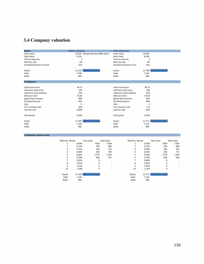
130
3.4 Company valuation
Merton Before&refinacing After&refinancingAsset&value 19.394 Morgan&Stanley&2008&report Asset&value 19.394Debt&Value 9.224 Debt&Value 8.658Time&to&maturity 3 Time&to&maturity 3RiskGfree&rate 4% RiskGfree&rate 4%Standard&deviation&of&asset 25% Standard&deviation&of&asset 25%
Equity 11.220 87,65&€&per&share Equity 11.709 91,48&€&per&shareDebt 7.208 Debt 7.201ALRG 966 ALRG 484
Creditgrades
Initial&stock&price 94,73 Initial&stock&price 94,73reference&stock&price 100 reference&stock&price 100reference&stock&valatility 33% reference&stock&valatility 33%debt&per&share 72,06 debt&per&share 67,64global&debt&recovery 50% global&debt&recovery 50%SD&default&barrier 30% SD&default&barrier 30%time 3 time 3Firm&recovery&rate 30% Firm&recovery&rate 0,3riskGfree&rate 4,00% riskGfree&rate 0,04
CDS&Spread 0,29% CDS&Spread 0,25%
Equity 11.284 88,16&€&per&share Equity 11.757 91,85&€&per&shareDebt 7.144 Debt 7.153ALRG 966 ALRG 484
Creditgrades (spread curve)
Maturity Spread Face&value Real&value Maturity Spread Face&value Real&value1 0,04% 3420 3.284 1 0,03% 3420 3.2852 0,15% 959 883 2 0,12% 959 8833 0,31% 183 161 3 0,26% 183 1614 0,48% 920 769 4 0,42% 920 7715 0,64% 1772 1.405 5 0,58% 1772 1.4096 0,78% 836 627 6 0,72% 836 6307 0,91% 0 G 7 0,84% 0 G8 1,01% 0 G 8 0,95% 0 G9 1,10% 0 G 9 1,04% 0 G10 1,18% 0 G 10 1,12% 0 G
Equity 11.299 88,27&€&per&share Equity 11.771 91,96&€&per&shareDebt 7.130 Debt 7.139ALRG 966 ALRG 484
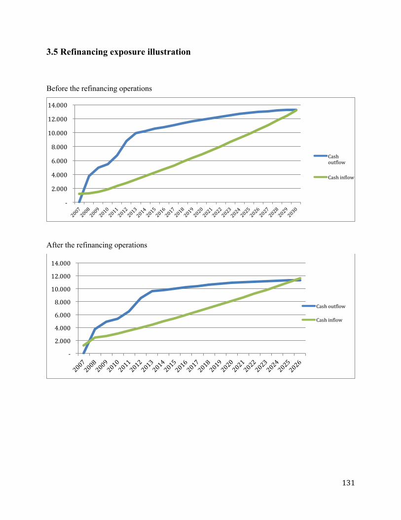
131
3.5 Refinancing exposure illustration
Before the refinancing operations
After the refinancing operations
-‐
2.000
4.000
6.000
8.000
10.000
12.000
14.000
Cash out]low
Cash in]low
-‐
2.000
4.000
6.000
8.000
10.000
12.000
14.000
Cash out]low
Cash in]low

132
4. TUI AG
4.1 Assumptions and data
Financial'projections'(in'€'million)Year%of%study 2009
Cash%at%t=0 300 ''''''''''2008'financial'report
FCF%forecast
2009 2010 2011 2012 2013 2014 2015
West'LB'02/09'report
532 '''''''''' 620 '''''''''' 774 '''''''''' 2.040 ''''''' 834 '''''''''' 849 '''''''''' 906 ''''''''''
Dividend%forecast
2009 2010 2011 2012 2013
West'LB'02/09'report
(124)''''''''' (125)''''''''' (175)''''''''' (201)''''''''' (213)'''''''''Debt%amorization
2009 2010 2011 2012 2013
(800)''''''''' (1.150)'''''' (800)''''''''' (1.800)'''''' (800)'''''''''2008'financial'report
Merton'model
Time%to%maturity 3 '''''''''''''''RiskCfree%rate 3,50%
CreditGrades'modelInitial%stock%price 8,05
reference%stock%price 8,05reference%stock%valatility 0,4debt%per%share 21,314741 21,314741global%debt%recovery 0,5percentage%standard%deviation%of%the%default%barrier.%0,3Firm%recovery%rate 0,5
Refinancing'gapBefore After
CDS 12,00% 23,00%number%of%share%at%t=0%(M) 251 251
average%yield 4,6%Credit%premium 8,96% 17,98%
FCF%Growth%rate 2%Dividend%growth%rate 2%
debt%actualization%cost%(kd) 4,57%Tax%rate 18,00%
Refinancing'operations'(M€)2009 2010 2011 2012 2013
Asset%disposals 1.600 '''''''
Own'computation
assumptionassumption
Annual'report'(last'debt'issue)
Annual'report
assumptionassumptionCredit'Suisse
BloombergAnnual'report
Annual'report
Average'weighted'maturityBloomberg
Bloomberg
West'LB'02/09'report
BloombergOwn'computation'

133
4.2 Projection of cash inflow / outflow
Assets
2008
2009
2010
2011
2012
2013
2014
2015
2016
2017
2018
2019
2020
Sur
plus
cas
h30
0-
--
--
Ope
ratin
g FC
F53
262
077
42.
040
834
849
906
953
987
1.02
71.
073
1.07
0D
ivid
ends
(124
)(1
25)
(175
)(2
01)
(213
)(2
17)
(222
)(2
26)
(231
)(2
35)
(240
)(2
45)
Liabilities
Inte
rest
exp
ense
(244
)(2
08)
(155
)(1
19)
(37)
-D
ebt a
mor
tizat
ion
(800
)(1
.150
)(8
00)
(1.8
00)
(800
)-
--
-

134
4.3 Refinancing gap computation
Ref
inan
cing
gap
val
uatio
n-
W/o$cap
ital$cha
nges
2008
2009
2010
2011
2012
2013
2014
2015
2016
2017
2018
2019
2020
2021
2022
2023
Cum
ulat
ed li
abili
ties
-1.
044
2.45
53.
604
5.80
26.
974
7.39
47.
781
8.12
38.
405
8.61
38.
731
8.73
78.
737
8.73
78.
737
Cum
ulat
ed F
CF
300
708
1.20
31.
802
3.64
14.
262
4.89
45.
578
6.30
57.
062
7.85
38.
686
9.51
210
.364
11.2
4512
.155
Ann
ual R
G30
0(6
36)
(915
)(5
50)
(359
)(5
51)
211
297
385
475
584
715
818
853
881
910
Cum
ulat
ed R
G30
0(3
36)
(1.2
52)
(1.8
02)
(2.1
61)
(2.7
12)
(2.5
00)
(2.2
03)
(1.8
18)
(1.3
43)
(760
)(4
4)77
41.
627
2.50
73.
417
Cos
t of t
he R
G(3
0)(1
12)
(162
)(1
94)
(243
)(2
24)
(197
)(1
63)
(120
)(6
8)(4
)-
--
-A
ctua
lizat
ion
fact
or0,
840,
870,
910,
961,
001,
051,
091,
141,
201,
251,
311,
371,
431,
501,
56A
ctua
lized
RG
val
ue(3
6)(1
28)
(177
)(2
03)
(243
)(2
14)
(181
)(1
42)
(101
)(5
4)(3
)-
--
-
With
$cap
ital$cha
nges$
2008
2009
2010
2011
2012
2013
2014
2015
2016
2017
2018
2019
2020
2021
2022
2023
Cum
ulat
ed li
abili
ties
-1.
644
2.37
53.
330
5.32
06.
243
6.40
16.
418
Cum
ulat
ed F
CF
300
1.97
62.
451
3.06
44.
993
5.64
66.
339
7.05
4A
nnua
l RG
300
32(2
56)
(342
)(6
0)(2
70)
535
699
Cum
ulat
ed R
G30
033
276
(266
)(3
27)
(597
)(6
2)63
7C
ost o
f the
RG
--
(48)
(59)
(107
)(1
1)-
Act
ualiz
atio
n fa
ctor
0,84
0,87
0,91
0,96
1,00
1,05
1,09
Act
ualiz
ed R
G v
alue
--
(52)
(61)
(107
)(1
1)-
W/O
With
In
trisi
c A
LRG
(TM
) val
ue(1
.482
)(2
32)
Tim
e va
lue
fact
or1,
471,
27A
LRG
(TM
) val
ue(2
.179
)(2
94)

135
4.4 Company valuation
Merton Before&Refinancing After&RefinancingAsset&value 7.850 Asset&value 7.000Debt&Value 7.529 Debt&Value 5.644Time&to&maturity 3 Time&to&maturity 3RiskDfree&rate 3,5% RiskDfree&rate 3,5%Standard&deviation&of&asset 20% Standard&deviation&of&asset20%
Equity 1.684 6,71&€&per&share Equity 2.154 8,58&€&per&shareDebt 4.212 Debt 4.583ALRG 1.954 ALRG 263
Creditgrades simplified
Initial&stock&price 8,05 Initial&stock&price 8,05reference&stock&price 8,05 reference&stock&price 8,05reference&stock&valatility 40% reference&stock&valatility40%debt&per&share 29,10 debt&per&share 22,36global&debt&recovery 50% global&debt&recovery 50%SD&default&barrier 30% SD&default&barrier 30%time 3,12 time 3,12Firm&recovery&rate 50% Firm&recovery&rate 50%riskDfree&rate 4% riskDfree&rate 3,50%
CDS&Spread 4,44% CDS&Spread 3,30%
Equity 1.721 6,86&€&per&share Equity 2.410 9,6&€&per&shareDebt 4.175 Debt 4.326ALRG 1.954 ALRG 263
Creditgrades complete
Maturity Spread Face&value Real&value Maturity Spread Face&value Real&value1 8,20% 800 712 1 4,83% 800 7362 5,45% 1150 962 2 3,69% 1150 9963 4,52% 800 629 3 3,33% 800 6524 4,04% 1800 1.332 4 3,15% 1800 1.3805 3,74% 800 557 5 3,03% 800 5776 3,52% 6 2,94%7 3,36% 7 2,87%8 3,24% 8 2,80%9 3,13% 9 2,75%10 3,04% 10 2,70%
Equity 1.705 6,79&€&per&share Equity 2.396 9,55&€&per&shareDebt 4.191 Debt 4.341ALRG 1.954 ALRG 263

136
4.5 Refinancing exposure illustration
Before the refinancing operations
After the refinancing operations
-‐ 1.000 2.000 3.000 4.000 5.000 6.000 7.000 8.000 9.000 10.000
2008 2009 2010 2011 2012 2013 2014 2015 2016 2017 2018 2019 2020
Cash out]low
Cash in]low
-‐
1.000
2.000
3.000
4.000
5.000
6.000
7.000
8.000
2008 2009 2010 2011 2012 2013 2014 2015 2016 2017 2018 2019 2020
Cash out]low
Cash in]low

137
5. KPN
5.1 Assumptions and data
Financial'projections'(in'€'million)Year%of%study 2013
Cash%at%t=0 947 '''''''''''''2012'financial'report
FCF%forecast2013 2014 2015 2016 2017 2018 2019 ING'01/13'report1.000 ''''''''' 1.100 ''''''' 1.150 ''''''' A ''''''''''' A ''''''''''' A ''''''''''' A '''''''''''
Dividend%forecast2013 2014 2015 ING'01/13'report(300)''''''''''' (300)''''''''' (300)'''''''''
Debt%amorization2013 2014 2015 2016 2017 2014
(1.100)'''''''' (1.400)'''''' (1.000)'''''' (1.300)'''''' (1.000)'''''' (1.300)''''''2012'financial'report
2016 2017 2018 2019 2020 2014
(1.000)'''''''' (1.500)'''''' (1.300)'''''' (800)''''''''' (500)''''''''' (3.100)''''''
Merton'modelTime%to%maturity 10 '''''''''''''''RiskFfree%rate 2,50%
CreditGrades'modelInitial%stock%price 2,54reference%stock%price 2,54reference%stock%valatility 27%debt%per%share 11 4global%debt%recovery 50%percentage%standard%deviation%of%the%default%barrier.%30%Firm%recovery%rate 40%
Refinancing'gapBefore After
CDS 1,60% 1,60%number%of%share%at%t=0%(M) 1400 4200
average%yield 5,3%Credit%premium A1,00% A1,00%
FCF%Growth%rate 3%Dividend%growth%rate 0%debt%actualization%cost%(kd) 5%Tax%rate 17,00%
Refinancing'operations'(M€)2009 2010 2011 2012 2013
Own'computation
assumptionassumption
Annual'report'(last'debt'Annual'report
assumptionassumptionCredit'Suisse
BloombergAnnual'report
Annual'report
Average'weighted'Bloomberg
BloombergING'01/13'report
BloombergOwn'computation'

138
5.2 Projection of cash inflow / outflow
Assets
2012
2013
2014
2015
2016
2017
2018
2019
2020
2021
2022
2023
2024
2025
2026
2027
2028
2029
2030
2031
2032
Sur
plus
cas
h94
7-
--
--
Ope
ratin
g FC
F1.
000
1.10
01.
150
1.18
51.
220
1.25
71.
294
1.33
31.
373
1.41
41.
457
1.50
01.
546
1.59
21.
640
1.68
91.
739
1.79
21.
845
1.90
1D
ivid
ends
(300
)(3
00)
(300
)(3
00)
(300
)(3
00)
(300
)(3
00)
(300
)(3
00)
(300
)(3
00)
(300
)(3
00)
(300
)(3
00)
(300
)(3
00)
(300
)(3
00)
Liabilities
Inte
rest
exp
ense
(673
)(6
25)
(563
)(5
19)
(462
)(4
18)
(361
)(3
17)
(251
)(1
94)
(158
)(1
36)
Deb
t am
ortiz
atio
n(1
.100
)(1
.400
)(1
.000
)(1
.300
)(1
.000
)(1
.300
)(1
.000
)(1
.500
)(1
.300
)(8
00)
(500
)(3
.100
)

139
5.3 Refinancing gap computation
Ref
inan
cing
gap
val
uatio
n-
W/o$cap
ital$cha
nges
2012
2013
2014
2015
2016
2017
2018
2019
2020
2021
2022
2023
2024
2025
2026
2027
2028
2029
2030
2031
2032
Cum
ulat
ed li
abili
ties
-1.
773
3.80
35.
422
7.32
88.
919
10.7
9312
.348
14.3
8216
.191
17.4
7218
.426
21.9
4922
.331
22.6
7822
.986
23.2
5123
.471
23.6
4123
.756
23.8
13C
umul
ated
FC
F94
71.
647
2.44
73.
297
4.18
25.
102
6.05
87.
053
8.08
69.
159
10.2
7311
.430
12.6
3013
.876
15.1
6816
.507
17.8
9619
.336
20.8
2722
.373
23.9
74A
nnua
l RG
947
(1.0
73)
(1.2
30)
(769
)(1
.022
)(6
71)
(918
)(5
61)
(1.0
01)
(736
)(1
68)
203
(2.3
23)
863
945
1.03
21.
123
1.22
01.
322
1.43
01.
544
Cum
ulat
ed R
G94
7(1
26)
(1.3
56)
(2.1
25)
(3.1
46)
(3.8
17)
(4.7
35)
(5.2
95)
(6.2
96)
(7.0
32)
(7.1
99)
(6.9
96)
(9.3
19)
(8.4
55)
(7.5
10)
(6.4
78)
(5.3
55)
(4.1
35)
(2.8
13)
(1.3
83)
161
Cos
t of t
he R
G1
1421
3138
4753
6370
7270
9384
7565
5341
2814
-A
ctua
lizat
ion
fact
or0,
810,
860,
900,
951,
001,
051,
111,
171,
231,
291,
361,
441,
511,
591,
681,
761,
861,
962,
062,
17A
ctua
lized
RG
val
ue2
1623
3338
4548
5457
5551
6556
4738
3022
147
-
With
$cap
ital$cha
nges$
2012
2013
2014
2015
2016
2017
2018
2019
2020
2021
2022
2023
2024
2025
2026
2027
2028
Cum
ulat
ed li
abili
ties
-1.
773
3.79
85.
361
7.18
08.
642
10.3
6011
.733
13.5
7715
.189
16.2
6617
.006
20.3
0720
.458
20.5
6420
.621
20.6
26C
umul
ated
FC
F94
75.
647
6.44
77.
297
8.18
29.
102
10.0
5811
.053
12.0
8613
.159
14.2
7315
.430
16.6
3017
.876
19.1
6820
.507
21.8
96A
nnua
l RG
947
2.92
7(1
.225
)(7
13)
(935
)(5
42)
(761
)(3
79)
(811
)(5
39)
3841
7(2
.101
)1.
095
1.18
61.
282
1.38
4C
umul
ated
RG
947
3.87
42.
649
1.93
61.
002
460
(301
)(6
80)
(1.4
92)
(2.0
30)
(1.9
93)
(1.5
76)
(3.6
77)
(2.5
82)
(1.3
96)
(113
)1.
271
Cos
t of t
he R
G-
--
--
37
1520
2016
3726
141
-A
ctua
lizat
ion
fact
or0,
810,
860,
900,
951,
001,
051,
111,
171,
231,
291,
361,
441,
511,
591,
681,
76A
ctua
lized
RG
val
ue-
--
--
36
1316
1512
2617
91
-
W/O
With
(Apr
il)In
trisi
c R
G v
alue
701
117
Tim
e va
lue
fact
or1,
271,
27R
G v
alue
887
148

140
5.4 Company valuation
Merton Before&Refinancing After&RefinancingAsset&value 15.979 Asset&value 19.979Debt&Value 14.413 Debt&Value 15.152Time&to&maturity 10 Time&to&maturity 4RiskCfree&rate 3% RiskCfree&rate 3%Standard&deviation&of&asset 14% Standard&deviation&of&asset 14%
Equity 5.431 3,88&€&per&share Equity 6.478 1,54&€&per&shareDebt 11.243 Debt 13.635ALRG (695) ALRG (134)
Creditgrades simplified
Initial&stock&price 2,54 Initial&stock&price 2,54reference&stock&price 2,54 reference&stock&price 2,54reference&stock&valatility 27% reference&stock&valatility 27%debt&per&share 11,74568709 debt&per&share 3,69global&debt&recovery 50% global&debt&recovery 50%SD&default&barrier 30% SD&default&barrier 30%time 10 time 10Firm&recovery&rate 50% Firm&recovery&rate 50%riskCfree&rate 3% riskCfree&rate 3%
CDS&Spread 2,29% CDS&Spread 0,83%
Equity 7.088 5,06&€&per&share Equity 11.943 2,84&€&per&shareDebt 9.586 Debt 8.170ALRG (695) ALRG (134)
Creditgrades complete
Maturity Spread Face&value Real&value Maturity Spread Face&value Real&value1 11,32% 1100 958 1 0,39% C2900 (2.817)2 6,32% 1400 1.174 2 0,43% 1400 1.3203 4,65% 1000 807 3 0,50% 1000 9144 3,81% 1300 1.010 4 0,57% 1300 1.1505 3,30% 1000 748 5 0,63% 1000 8556 2,96% 1300 937 6 0,69% 1300 1.0747 2,72% 1000 694 7 0,73% 1000 7988 2,53% 1500 1.003 8 0,77% 1500 1154,638929 2,38% 1300 838 9 0,80% 1300 965,60469910 2,27% 800 497 10 0,83% 800 573,31137211 2,17% 500 299 11 0,86% 500 345,69109112 2,09% 3100 1.788 12 0,87% 3100 2067,72048
Equity 5.922 4,36&€&per&share Equity 11.713 2,81&€&per&shareDebt 10.752 Debt 8.400ALRG (695) ALRG (134)

141
5.5 Refinancing exposure illustration
Before the refinancing operations
After the refinancing operations
-‐
5.000
10.000
15.000
20.000
25.000
30.000
2012
2013
2014
2015
2016
2017
2018
2019
2020
2021
2022
2023
2024
2025
2026
2027
2028
2029
2030
2031
2032
Cash out]low
Cash in]low
-‐
5.000
10.000
15.000
20.000
25.000
Cash in]low
Cash out]low

142