field theoretical approach to the paramagnetic-ferrimagnetic transition in strongly coupled...

*Corresponding author. Tel.: #212-2-704672; fax: #212-2-704675.

E-mail address: [email protected] (M. Be-nhamou).

Journal of Magnetism and Magnetic Materials 213 (2000) 219}233

Field theoretical approach to the paramagnetic-ferrimagnetictransition in strongly coupled paramagnetic systems

M. Chahid, M. Benhamou*

Laboratoire de Physique des Polyme% res et Phe&nome%nes Critiques, B.P. 7955, Faculte& des Sciences Ben M'sik, Casablanca, Morocco

Received 5 February 1999; received in revised form 20 July 1999

Abstract

The aim of this paper is the investigation of the critical properties of two strongly coupled paramagnetic sublatticesexhibiting a paramagnetic}ferrimagnetic transition, at some critical temperature ¹

#greater than the room temperature.

In order to take into account the strong #uctuations of the magnetization near the critical point, use is made of therenormalization-group (RG) techniques applied to an elaborated "eld model describing such a transition, which is ofLandau}Ginzburg}Wilson type. The associated free energy or action is a functional of two kinds of order parameters(local magnetizations), which are scalar "elds u and t relative to these sublattices. It involves quadratic and quartic termsin both "elds, and a lowest-order coupling C

0ut, where C

0'0 stands for the coupling constant measuring the

interaction between the two sublattices. We "rst show that the associated "eld theory is renormalizable at any order ofthe perturbation series in the coupling constants, up to a critical dimension d

#"4, and that, the corresponding

counterterms have the same form as those relative to the usual u4-theory (C0"0). The existence of the renormalization

theory enables us to write the RG-equations satis"ed by the correlation functions. We solve these using the standardcharacteristics method, to get all critical properties of the system under investigation. We "rst determine the exact shapeof the critical line in the (¹, C)-plane, along which the system undergoes a phase transition. Second, we determine thescaling laws of the correlation functions, with respect to relevant parameters of the problem, namely, the wave vector q,the (renormalized) coupling C and the temperature shift ¹!¹

#. We "nd that these scaling laws are characterized by

critical exponents, which are the same as those relative to Ising-like magnetic systems. ( 2000 Elsevier Science B.V. Allrights reserved.

PACS: 05.70.Fh; 75.50.Gg; 05.70.Jk

Keywords: Sublattices; Coupling; Paramagnetism; Ferrimagnetism; Transition; Renormalization-group; Critical-line; Correlations;Scaling laws

1. Introduction

The so-called super-weak ferrimagnetic materialswe consider here are of considerable technologicalimportance, specially, in the domain of energystocking (long-life lithium batteries). Amongthese, we can quote certain members of Heusler

0304-8853/00/$ - see front matter ( 2000 Elsevier Science B.V. All rights reserved.PII: S 0 3 0 4 - 8 8 5 3 ( 9 9 ) 0 0 8 0 3 - 3

Pauli-paramagnetic alloys [1] based on the com-position X

2YZ, with (X"Pd, Cu; Y"Ti, V and

Z"Al, In, Sn). Also, we can quote the recent lamel-lar Curie}Weiss paramagnetic compounds [2], likeAM

xM@

1~xO

2(0)x(1) with (A"Li, Na, K; M,

M@"N, Co,2). For all these materials, theferrimagnetic order takes place below somecritical temperature ¹

#, greater than room temper-

ature.To describe the super-weak ferrimagnetism aris-

ing from such materials, a continuous model basedon the Landau theory [3}5] was proposed recentlyby Neumann and co-workers [6]. This model as-sume that the material consists of a lattice made oftwo coupled Pauli or Curie}Weiss paramagneticsublattices [7,8], with respective local magneti-zations u and t. Above the critical temperature ¹

#,

both magnetizations vanish and the system isa paramagnet. Below this temperature, an anti-parallel con"guration of the magnetizations isfavored, but with non-vanishing overall magneti-zation. One can say that the material exhibits a fer-rimagnetic state. The appearance of such an order isintimately related to the existence of a strong coup-ling between the two sublattices. Quantitatively,this coupling manifests itself through the introduc-tion of an extra term C

0ut in the free energy (see

below). Positive values of the coupling constantC

0favor the antiparallel alignment of the local

moments u and t, and then, the ferrimagneticorder appears.

From a mean-"eld point of view, the theory hasbeen developed through, "rst, some numericalmethod [6], and second, through an exactanalytic analysis [9,10]. However, the mean-"eldapproach underestimates the strong #uctuations ofthe local moments near the critical point. To gobeyond this approximation, and in order to geta correct critical behavior, we will use the RG-techniques [5,11}13] applied to the present "eldmodel.

Our results are the following. We "rst show thatthe associated "eld theory, whose action is thatdescribed below, is renormalizable at any order ofthe perturbation series in the coupling constants,and that, the necessary counterterms to removeshort-range divergences are similar to those of theusual u4-theory (C

0"0). Thus, no new counter-

term is needed to renormalize the coupling con-stant C

0. Second, we reexamine the critical behav-

ior of the mean-"eld two-point correlationfunction, with respect to relevant parameters of theproblem, namely, the wave vector q, the temper-ature shift ¹!¹

#and the (renormalized) coupling

constant C. Taking advantage of the existence ofthe renormalization theory, we write the RG-equa-tions satis"ed by the correlation functions. Usingthe standard characteristics method [11}13], wesolve these, to get all critical properties of the sys-tem. Also, we determine the exact shape of thecritical line, along which the system undergoesa phase transition, in the (¹

#,C)-plane. We "nd

that this line is given by the power law: t#+C1@c,

where c is the critical exponent of Ising-likesystems [12,13], which characterizes the behaviorof the magnetic susceptibility. There, t is thetemperature parameter de"ned below. In fact,this line separates two domains, paramagneticand ferrimagnetic. Finally, we determine allscaling laws of the correlation functions,with respect to the relevant parameters of the prob-lem.

This paper is organized as follows. Section 2 isdevoted to a succinct presentation of the used "eldmodel, and to the construction of the associateda-parametrization. Section 3 is devoted to theproof of the renormalizability of the theory.We reexamine, in Section 4, the mean-"eld criticalbehavior of the system. The determination of thecritical line shape and the scaling laws of correla-tion functions, solving the RG-equations, are theaims of Section 5. We draw some concluding re-marks in Section 6. The passage from the discretemodel to the continuous one is presented in theappendix.

2. The 5eld model

The physical system we consider here is de-scribed by two kinds of order parameters, whichare scalar "elds u(x) and t(x) de"ned on the d-dimensional Euclidean space. The free energy oraction enables one to investigate the para}fer-rimagnetic transition within this system writes

220 M. Chahid, M. Benhamou / Journal of Magnetism and Magnetic Materials 213 (2000) 219}233

[6,9,10]

H[u, t]

kB¹

"Pd$x C1

2(+u)2#

1

2(+t)2#

a02

u2#A

02

t2

#C0ut#

u0

4!(u2)2#

v0

4!(t2)2D(x),

(2.1)

here, ¹ is the absolute temperature and kB

theBoltzmann constant. The coupling constantsu0

and v0

are taken to be positive, to ensure thestability of this free energy. The coe$cients a

0and

A0

or &square masses' are temperature dependent.Their temperature dependence is as follows:

a0(¹)"a

1#b

1¹2, A

0(¹)"a

2#b

2¹2 (2.2)

for a Pauli paramagnet [7,8], or

a0(¹)"a6 (¹!h

1), A

0(¹)"AM (¹!h

2) (2.3)

for a Curie}Weiss paramagnet [8,14]. The coe$-cients a

iand b

iappearing in Eq. (2.2) have a simple

dependence in both free electron density and Fermienergy relative to the two sublattices [15]. In Eq.(2.3), h

1and h

2stand for the Curie}Weiss temper-

atures, and we show that they are proportional toexchange integrals J

1'0 and J

2'0 inside the

sublattices (see the appendix).In the free energy expression (2.1), appears an

extra term C0ut, which represents the lowest-order

interaction between the two sublattices, with re-spective local moments or "elds u and t. In fact,such a term has the same e!ect as an internalmagnetic "eld. Positive values of the couplingC

0(C

0'0) favor the antiparallel con"gurations of

moments u and t, while its negative values(C

0(0) favor rather their parallel alignment. In

the case of Curie}Weiss materials, like lamellarcompounds [2,16], the coupling C

0has a simple

meaning. As a matter of fact, we show, in Appendix,that C

0is proportional to exchange integral

J12

(0 between the two sublattices. In this work,we are concerned only with positive values of C

0,

for which appears a ferrimagnetic order at lowtemperature. In addition, this coupling will be as-sumed to be constant in all temperature-rangearound the critical point. The subscripts on a

0, A

0,

C0, u

0and v

0are used to distinguish these bare

parameters from the corresponding renormalizedones a, A, C, u and v, de"ned later.

The "eld theory of action (2.1) is a generalizationof the usual one-component u4-theory. The di!er-ence comes from the fact that, in the present case,we have several masses and coupling constants anda quadratic coupling of "elds u and t. A dimen-sional analysis shows that: [a

0]"[A

0]" [C

0]"

¸~2, [u0]"[v

0]"¸d~4 and [u]"[t]"¸1~d@2,

where ¸ is some length. The coupling constantsu0and v

0become marginal at the critical dimension

d#"4 of the system.As usual, various physical quantities can be ex-

pressed in terms of (connected) correlation func-tions, which are the vacuum expectation value ofproducts of "elds u and t. In reciprocal space, theFourier transform of the (N#M)-point connectedcorrelation function made of Nu and Mt is givenby

G(N,M)(qi;a

0, A

0,C

0,u

0, v

0)"T

N<i/1

N`M<

j/N`1

uqitqjU

#0//.(2.4)

with the scattering wave vector global conserva-tion, i.e. +

iqi"0, which is a direct consequence of

the translation symmetry. In de"nition (2.4), uq

isthe Fourier transform of "eld u(x). The particularcase where N#M"2 corresponds to the partialpair-correlation functions (or structure factors) be-tween the two magnetic species with respective mo-ments u and t, namely G(2,0)(q;2), G(0,2)(q;2)and G(1,1)(q;2). We note that the zero scattering-angle limit (q"0) of these two-point correlationfunctions yields the three partial magnetic suscep-tibilities s

NM, i.e. G(N,M)(q"0)"k

B¹s

NM, with

N#M"2.Correlation functions G(N,M)s can be expanded

with respect to the coupling constants u0

and v0,

and described in terms of Feynman diagrams.

2.1. Feynman rules

These rules are similar to those of the usualu4-theory (C

0"0), with the only di!erence that,

in the present case, we have three kinds of

M. Chahid, M. Benhamou / Journal of Magnetism and Magnetic Materials 213 (2000) 219}233 221

propagators [9], namely

G(2,0)0

(k)"1

k2#a0!(C2

0/(k2#A

0))

(2.5a)

G(0,2)0

(k)"1

k2#A0!(C2

0/(k2#a

0))

(2.5b)

G(1,1)0

(k)"C

0(k2#a

0)(k2#A

0)!C2

0

. (2.5c)

Let G be a connected Feynman diagram with< vertices, I,I

1#I

2#I

3oriented internal lines,

E external legs and ¸ loops. I1, I

2and I

3are

respectively the numbers of internal lines of propa-gators G(2,0), G(0,2) and G(1,1). We denote by P

vthe

algebraic sum of external wave vectors outgoingfrom the vertex v. We will need the <]I incidencematrix (e

vl) that is de"ned as usual by [17,18]:

evl

equals #1, if the line l starts from the vertexv,!1 if it ends at v, and 0, otherwise. (By conven-tion, e

vl"0, if l is a loop line, i.e. which starts and

ends at the same vertex v). Then, the Feynmanamplitude of the diagram G, expressed in the d-dimensional wave vector space, writes

I(Pv, a

0, A

0, C

0)"P

`=

~=

I<l/1

Addk

l(2p)dB G<

l|J1

G(2,0)0

(kl)

]<l|J2

G(0,2)0

(kl)<l|J3

G(1,1)0

(kl)

]V~1<v/1

(2p)dddAPv

#

I+l/1

evlklBH

.

(2.6)

We have ignored the symmetry factor, the couplingconstants and external propagators. J

1, J

2and

J3

denote the sets of internal lines of propagatorsG(2,0), G(0,2) and G(1,1), respectively.

2.2. a-parametric representation

It is well known that the a-parametrization[17}21] is a very useful method to make calcu-lation in quantum "eld theory [17] and criticalphenomena [5,12,13]. Its extension to the presenttheory is straightforward. To do this, it will bemade use of the following representation of the

three propagators

1

k2#a0!(C2

0/(k2#A

0))

"P=

0

da m1(a)e~a*k2`(a0À0 )@2+, (2.7a)

1

k2#A0!(C2

0/(k2#a

0))

"P=

0

dam2(a)e~a*k2`(a0À0 )@2+, (2.7b)

C0

(k2#a0)(k2#A

0)!C2

0

"P=

0

da m3(a)e~a*k2`(a0À0 )@2+, (2.7c)

where

m1(a)"cosh(ga)!

a0!A

02g

sinh(ga), (2.7d)

m2(a)"cosh(ga)!

A0!a

02g

sinh(ga), (2.7e)

m3(a)"

C0

gsinh(ga), (2.7f)

g"SAa0!A

02 B

2#C2

0.

(2.7g)

Now, it is possible to construct an a-parametricrepresentation for the present theory. To this end,the "rst step consists in replacing the propagatorsin Eqs. (2.5a)}(2.5c) by their integral representationEqs. (2.7a)}(2.7g) and the Dirac distributions d

$s

expressing the moment conservation at vertices bytheir Fourier transform. Without details, we givethe expected a-parametrization of the Feynmanamplitude

I(Pv, a

0, A

0, C

0)"P

`=

0

I<l/1

[dale~al a6 ]m(a)Z(P

v, a),

(2.8a)


where

a6 ,a0#A

02

, (2.8b)

m(a)"<l|J1

m1(a

l)<l|J2

m2(a

l)<l|J3

m3(a

l), (2.8c)

Z(Pv, a)"(4p)~Ld@2[P

G(a)]~d@2

]expG!V~1+

v,v{/1

Pv[d~1

G(a)]

vv{P

v{H. (2.8d)

Here

[dG(a)]

vv{"

I+l/1

evlev{l

al

, v, v@"1,2,<!1 (2.8e)

and

PG(a)"

I<l/1

aldet[d

G(a)] (2.8f)

stand, respectively, for the (<!1)](<!1) matrixand the polynomial of Symanzik [17].

We note that expression (2.8a) shows that thea-integrand of the present "eld theory di!ers fromthe usual one (with C

0"0), with square mass

a6 "(a0#A

0)/2, only by the presence of the func-

tion m(a) that contains all dependence on C0.

3. Renormalization

3.1. Power-counting

To analyze short-range divergences, it will besu$cient to consider only the proper or one-par-ticle irreducible (1PI) diagrams. Consider a 1PIdiagram G of ¸ loops, < vertices and I"I

1#

I2#I

3internal lines. I

1, I

2and I

3stand, respec-

tively, for the numbers of internal lines havingG(2,0), G(0,2) and G(1,1) as propagators. To analyzethese divergences, the starting point is the Feynmanamplitude expressed in the a-parametrization givenby Eq. (2.8a). After some calculation, we "nd thatthe superxcial degree of divergence (s.d.d.) of G isgiven by

u(G)"¸d!2I!2I3,u

0(G)!2I

3. (3.1)

Diagrams whose u(G)*0 are said to be superx-cially divergent, those for which u(G)(0, super"-cially convergent. u

0(G)"¸d!2I is the s.d.d. of

a diagram of the usual u4-theory having the sametopology as G. We "rst remark that the presence ofpropagators of type G(1,1)

0reduces the s.d.d. by

a 2I3

factor. Consequently, this same presence im-proves the convergence of the Feynman integral.

Now, we de"ne a subdiagram c of a diagram G asa subset of vertices of G and of all internal linesconnected to them in G. The corresponding s.d.d. isdenoted by u(c)"¸(c)d!2I(c)!2I

3(c). Accord-

ing to the regularity property of the function m(a)and using the standard Hepps' sectors techniques[22], we show that if u(c)(0, for all subdiagramsc of G, then the Feynman integral corresponding toG, Eq. (2.6), is absolutely convergent. This is theConvergence Theorem.

The analysis of the sign of the s.d.d. u, de"ned byEq. (3.1), permits us to select the vertex functionsprimitively divergent. These are made of IN"

N#M "elds u and t, eventually with insertions ofI¸"¸

1#¸

2#¸

3quadratic composite oper-

ators u2, t2 or ut. Here ¸1, ¸

2and ¸

3are the

respective numbers of these operators. We have theuseful topological relations [17]

4<4#3I¸"2I#E, (3.2a)

¸"I!<#1, (3.2b)

here, E"IN#I¸, <"<4#I¸ and I stand, re-

spectively, for the total numbers of external legs,vertices and internal lines. <

4being the total num-

ber of vertices of types (u2)2 and (t2)2. Combineexpression (3.1) of the s.d.d. and topological rela-tions (3.2a) and (3.2b), to get at d"4

u"4!IN!2I¸!2I3. (3.3)

The above formula is independent of the number ofvertices <

4(only at d"4).

In fact, we have three situations with u*0:(i) IN"2 and I¸"0: This corresponds to

u"2!2I3. Diagrams super"cially divergent are

such that I3"0 or I

3"1. For I

3"0, u"2, for

all diagrams for which internal lines have G(2,0)0

orG(0,2)

0as propagators. For I

3"1, u"0, for those

diagrams of which among their propagators, there


exists only one propagator of type G(1,1)0

. However,there is no 1PI diagram with I

3O0, which contains

only one propagator of type G(1,1)0

. Diagrams withI3*2 correspond to u(0. Consequently, no

counter-term proportional to the coupling con-stant C

0is needed to renormalize the theory.

(ii) IN"4 and I¸"0: This corresponds tou"!2I

3. Diagrams super"cially divergent are

such that I3"0 (u"0), that is those containing

only propagators of types G(2,0)0

or G(0,2)0

.(iii) IN"2 and I¸"1: This corresponds to

u"!2I3. Only those diagrams with I

3"0

which are super"cially divergent (u"0).In summary, the vertex functions primitively di-

vergent are:(a) The two-point vertex functions with no inser-

tions of composite operators u2, t2 or ut: IN"2and I¸"0 (with I

3"0).

(b) The two-point vertex functions with only oneinsertion of composite operators u2, t2 or ut:IN"2 and I¸"1 (with I

3"0).

(c) The four-point vertex functions with no inser-tions of composite operators u2, t2 or ut: IN"4and I¸"0 (with I

3"0).

Note that there are no short-range divergences,which come from the insertion of the compositeoperator ut. Indeed, we show that the renormali-zation of this latter is equivalent to a renormali-zation of the massive parameter C

0.

In consequence, to remove short-range divergen-ces up to d"4, it is su$cient to renormalize onlycorrelation functions (with I

3"0) described above,

that is for which (IN"2, I¸"0), (IN"2, I¸"1)with ¸

3"0 and (IN"4, I¸"0).

3.2. Dimensional renormalization

The connected correlation functions G(N,M)s canbe expanded with respect to the coupling constantsu0and v

0, and they exhibit short-range divergences.

The power-counting analysis pointed out pre-viously shows, in particular, that no C

0-dependent

counter-term is needed to remove a part of thesedivergences. The main question, now, is how torenormalize the theory. Before achieving this pro-gram, it is "rst necessary to regularize the theory.We decide to choose here the dimensional regular-ization with the minimal subtraction procedure of 't

Hooft and Veltman [23,24], with the regulatore"4!d (d

#"4 being the critical dimension of the

system). The spirit of this procedure is as follows.First, short-range divergences appear as poles ine"0, and second, the divergent part of the ampli-tude of any Feynman diagram is just the corre-sponding Laurent series in the regulator e. In fact,the last receipt plays the role of the renormalizationconditions, when one chooses other regularizationprocedures [17]. When the theory is renormaliz-able, the action expressed in terms of renormalizedxelds u

Rand t

R, and renormalized parameters a, A,

C, u and v, writes [23]

H[uR, t

R]

kB¹

"PddxC1

2(+u

R)2#

1

2(+t

R)2#

ak2

2u2

R

#

Ak2

2t2R#Ck2u

RtR

#

uke4!

(u2R)2#

vke4!

(t2R)2D(x), (3.4)

where a, A, C, u and v are, respectively, the renor-malized parameters corresponding to bare ones a

0,

A0, C

0, u

0and v

0. k is an arbitrary ('t Hooft) mass,

introduced in such a way that a, A, C, u and v bedimensionless irrespective of d. For instance, k canbe chosen to be the inverse of the lattice spacing.Recall that the addition of counter-terms to thisaction yields the bare action (2.1).

To prove the (multiplicative) renormalizability ofthe theory, we "rst consider the bare (connected)correlation function in the con"guration space,which is made of Nu and Mt "elds. This is de"nedas the vacuum expectation value

G(N,M)(xi, y

j; a

0, A

0, C

0, u

0, v

0; e)

"TN<k/1

M<l/1

u(xk)t(y

l)U

#0//.

(3.5)

that is calculated with the help of the free energyde"ned by Eq. (2.1).

The second step is based on the idea that consistsin developing formally the above correlation func-tion as a power series in the bare coupling constant


C0. In a straightforward way, we "nd

G(N,M)(xi, y

j; a

0, A

0, C

0, u

0, v

0; e)

"

=+

L/0

(!C0)L

¸! PL<l/1

ddzlG(N`L)

0

](xi, z

k; a

0, u

0; e)G(M`L)

0(y

j, z

k; A

0, v

0; e),

(3.6)

where

G(N`L)0

(xi, z

k; a

0, u

0)"T

N<l/1

L<m/1

u(xl)u(z

m)U

#0//.

,

(3.7)

G(M`L)0

(yj, z

k; A

0, v

0)"T

M<l/1

L<m/1

t(yl)t(z

m)U

#0//.

,

(3.8)

stand, respectively, for the correlation functions ofthe usual u4 and t4-theories taken separately, withrespective bare parameters (a

0, u

0) and (A

0, v

0).

Consequently, the relations between bare and re-normalized quantities are

u"[Zr (u; e)]1@2uR, t"[Zr (v; e)]1@2t

R, (3.9)

u0"keZ

u(u; e)u, v

0"keZ

u(v; e)v, (3.10)

a0"k2Z

a(u; e)a, A

0"k2Z

!(v; e)A, (3.11)

Zr , Za

and Zu, functions only of u (or v) and

e"4!d, are the "elds, masses and coupling con-stant renormalization factors, respectively. Theyare Laurent series in the regulator e and powersseries in u (or v): Z"1#+

ijaijuie~j where

i, j"1,2,R. Return to the usual correlation func-tions (3.7) and (3.8) and note that, each renormal-izes multiplicatively, and they contribute witha [Zr(u; e)](N`L)@2 and [Zr(v; e)](M`L)@2 factors, re-spectively. The fact that both correlation functions(3.7) and (3.8) renormalize multiplicatively impliesthe appearance of a global factor[Zr (u; e)]N@2[Zr (v; e)]M@2 in decomposition (3.6).The second implication is that, the bare couplingC

0renormalizes according to

C0"k2[Zr (u; e)Zr(v; e)]~1@2C. (3.12)

This renormalization equation must be viewed asa rede"nition of the coupling constant C

0. Hence,

the correlation functions G(N,M)s renormalize multi-plicatively according to the general formula

G(N,M)(qi; a

0, A

0, C

0, u

0, v

0; e)

"[Zr(u; e)]N@2[Zr(v; e)]M@2

]G(N,M)R

(qi; a, A, C, u, v, k, e). (3.13)

This is the expected result. The renormalizedcorrelation functions G(N,M)

Rs, as a function of e, is

free from singularities at e"0. Relationships (3.9)to (3.11) clearly show that the necessary counter-terms to remove short-range divergences are sim-ilar to those of the usual u4-theory. Result (3.13)can be extended to any arbitrary correlation func-tion with insertion of quadratic composite oper-ators u2, t2 or ut. We show that therenormalization of such operators is equivalent toa renormalization of massive parameters a

0, A

0and

C0, respectively. The former contributes by the re-

normalization factor [Za(u; e)]~1, the second by

[Za(v; e)]~1 and the last one by

[Zr (u; e)Zr (v; e)][email protected], it is important to point out that this

proof is independent of the regularization scheme.

4. Mean-5eld critical behavior

The starting point is the free energy de"ned byEq. (2.1), from which one can extract the expressionof the three two-point correlation functions,G(2,0)

0(q; 2), G(0,2)

0(q; 2) and G(1,1)

0(q; 2), using

the standard technique. We are concerned herewith the situation where the critical point is ap-proached from the above (disordered phase). In thiscase, we can keep only the quadratic part of the freeenergy, and the three correlation functions arethose given by Eqs. (2.5a)}(2.5c). They are func-tions, in particular, of the module q of the wavevector q. Expressions of these correlation functionsare valid only when the inequality a

0A

0'C2

0is

ful"lled, which is the condition de"ning the dis-ordered phase [9]. This inequality de"nes somerestricted domain in the (¹,C

0)-plane, since both

coe$cients a0(¹) and A

0(¹) depend on temper-

ature, Eqs. (2.2) or (2.3). Of course, in the C0"0

limit, G(1,1)0

"0, G(2,0)0

and G(0,2)0

reduce to theusual propagators (q2#a

0)~1 and (q2#A

0)~1,


Fig. 1. Mean-"eld critical line in the (t,C)-plane.

respectively. Expressions (2.5a)}(2.5c) tell us thatthe two-point correlation functions become singu-lar at q"0, when one is at the critical temperature¹

#de"ned through the equality [9]

a0(¹

#)A

0(¹

#)"C2

0. (4.1)

Therefore, to each value of the coupling C0

corre-sponds a transition temperature ¹

#(C

0). The above

equality de"ne a continuous critical line in the(¹, C

0)-plane.

Let us comment about equality (4.1) de"ning thecritical point. We "rst note that this equality meansthat the criticality does not emerge when botha0and A

0vanish. The criticality occurs rather when

a0, A

0and C

0are related by relation (4.1). Thus, we

can say that the system of free energy, Eq. (2.1),should not be regarded as two Ising-sublattices.Now, when there exists a critical temperature, thedisordered phase (¹'¹

#) is de"ned by the condi-

tion: a0(¹

#)A

0(¹

#)'C2

0, and the ordered or fer-

rimagnetic phase (¹(¹#) by: a

0(¹

#) A

0(¹

#)(C2

0.

Since, the ferrimagnetic state within these systemsappears above room temperature, then, from equal-ity (4.1), we can conclude that the phase transitionis possible only for high enough coupling constantC

0.It will be convenient to introduce the following

notations:

t0,Ja

0(¹)A

0(¹), t

#,Ja

0(¹

#)A

0(¹

#), (4.2)

t0

being the new temperature parameter. Withthese notations, the critical line, Eq. (4.1), becomes

t"C(0 , (/0"1). (4.3)

We have omitted the subscripts on t#

and C0. In

relation (4.3), /0

stands for some mean-"eld cross-over critical exponent. The shape of this critical line(¸

1), in the (t,C)-plane, is depicted in Fig. 1. This

line separates two distinct magnetic regions: para-magnetic (I) and ferrimagnetic (II).

Along the critical line where the material under-goes a phase transition, the associated structurefactors, at zero scattering-angle, diverge accordingto the power law

G(N,M)0

(q"0)&(t!t#)~c0 , (c

0"1). (4.4)

Remark that the singular behavior (4.4) is similar tothat obtained for the traditional para}ferromag-netic transition, with the same thermal critical ex-ponent c

0.

A detailed analysis of expressions (2.5a)}(2.5c)shows that, in the con"guration space and for largedistances, the two-point correlation functions de-crease exponentially as: exp(!r/m

0). It was found

[9] that the correlation length m0

diverges in thevicinity of the critical line as

m0&(t!t

#)~l0 , (l

0"1

2) (4.5)

and along this line (t"t#), the various structure

factors versus the module q of the wave vector q,behave according to

G(N,M)0

(q; t"t#)&1/q2~g0 , (g

0"0). (4.6)

This singular behavior is similar to the usual one,with the same thermal critical exponent g

0.

We note that, in the above critical behaviors(4.4)}(4.6), we have omitted the corresponding am-plitudes whose values are known. We also note thatthe subscripts on /

0, c

0, l

0and g

0are used to

distinguish these mean-xeld critical exponents fromthe correct ones, de"ned later.

Now, the aim is to derive the scaling laws for thestructure factors with respect to the relevant vari-ables, namely, the scattering wave vector q and thetemperature shift t!t

#. We are concerned only

with the situation where the system is in its critical


domain, that is around q"0 and t"t#. Using

their expressions (2.5a)}(2.5c), the structure factorscan be rewritten in the following scaling forms:

G(N,M)0

(q; a0, A

0, C

0, t!t

#)

"

1

(t!t#)c0

f (N,M)(q(t!t#)~l0 ; a

0(t!t

#)~1,

A0(t!t

#)~1, C

0(t!t

#)~1), (4.7)

G(N,M)0

(q; a0, A

0, C

0, t!t

#)

"

1

q2~g0h(N,M)((t!t

#)q~1@l0; a

0q~2, A

0q~2, C

0q~2)

(4.8)

with N#M"2. The scaling functions f (N,M) andh(N,M) are universal, their exact form can be ob-tained from expressions (2.5a)}(2.5c). Note that theappearance of the multiplicative power factorsx~j in equalities (4.7) and (4.8) means that thebehavior is controlled by the relevant parameterx (x"t!t

#, q).

To go beyond the mean-"eld approximation, it isnecessary to use the RG-techniques, in order toobtain a correct critical behavior. This is preciselythe aim of the following section.

5. Renormalization-group analysis

5.1. RG-equations

To derive the RG-equations, we take advantageof the independence of the bare correlation func-tions G(N,M)s on the scale mass k. We will denote bykLk D0 the l-derivatives at "xed bare parameters a

0,

A0, C

0, u

0and v

0. From kLk D0G(N,M)"0 and expres-

sion (3.13), we get the RG-equations

GkLk#=(u)Lu#=(v)L

v![2#g

a(u)]aL

a

![2#ga(v)]AL

A!

1

2[4!gr (u)!gr(v)]CL

C

#

N

2gr (u)#

M

2gr(v)H G(N,M)

R"0, (5.1)

where=(u)"kLk D0u stands for the Wilson functionand g

i(u)"kLk D0 ln[Z

i(u; e)], with i"a, u, for the

exponent functions. For example, to second orderin the coupling constant, they are given by theusual expansion [5]

=(u)"!eu#3u2!173u3#O(u4), (5.2)

gr(u)"16u2#O(u3), (5.3)

ga(u)"!u#5

6u2#O(u3), (5.4)

where e"4!d.Recall that the Wilson function=(u) may vanish

at some "xed value uH, that is =(uH)"0. To sec-ond order in e, one has [5]

uH"13e#17

81e2#O(e3). (5.5)

In fact, we have four kinds of "xed points, which are(0, 0), (uH, 0), (0, uH) and (uH, uH). The former is theGaussian "xed point, which is not relevant forphysics, because of the presence of the strong #uc-tuations of the order parameter near the criticalpoint. The "xed points (uH, 0) and (0, uH) are irrel-evant, since the two spin-sublattices are strongly#uctuating. Thus, (uH, uH) is the only infrared-stable"xed point, yielding a correct critical behavior.

Now, to solve the RG-equations (5.1), use will bemade of the standard characteristics method[5,11}13]. To this end, we introduce the followinge!ective variables a(l), A(l), C(l ), u(l) and v(l), whichare functions of the single scale parameter l, assolutions of the characteristic (or #ow) equations

ld

dlu(l)"=[u(l)], l

d

dlv(l)"=[v(l)], (5.6)

ld

dla(l)"!M2#g

a[u(l)]Na(l),

ld

dlA(l)"!M2#g

a[v(l)]NA(l), (5.7)

ld

dlC(l)"!

1

2M4!gr[u(l)]!gr[v(l)]NC(l) (5.8)

with the initial conditions u(l)"u, v(l)"v, a(l)"a,A(l)"A and C(l )"C. The above equations de-scribe how u, v, a, A and C transform if one changesthe mass scale k according to k(l)"kl. The


solutions of the #ow equations (5.7) and (5.8) arewritten as

a(l)"l~1@l Ea[u(l), u]a, A(l)"l~1@lE

a[v(l), v]A,

(5.9)

C(l)"l~c@l EC[u(l), u] )E

C[v(l), v]C (5.10)

with

Ea[u(l), u]"expG!P

u(l)

u

2#ga(u@)!l~1

=(u@)du@H,

(5.11)

EC[u(l), u]"expG!

1

2Pu(l)

u

2!gr (u@)!c/l=(u@)

du@H,(5.12)

where l and c are the usual thermal critical expo-nents relative to Ising-like systems [5,12,13]

l~1"2#ga(uH), c"l(2!g), g"gr (uH).

(5.13a)

We show that the general solution of the RG-equations (5.1) can be written as follows:

G(N,M)R

(qi; a, A, C, u, v, k)

"ldG`gG EG

G(N,M)R

(qi/l; a(l), A(l),C(l), u(l), v(l), k)

(5.13b)

with

EG[u(l), v(l); u, v]"expGP

u(l)

u

g1G

(u@)!gH1G

=(u@)du@H

]expGPv(l)

v

g2G

(v@)!gH2G

=(v@)dv@H,(5.14)

where

g1G

(u)"N

2gr (u), g

2G(v)"

M

2gr (v) (5.15)

and

gHG"

N#M

2g, gH

1G"

N

2g, gH

2G"

M

2g . (5.16)

In solutions (5.13a) and (5.13b), dG

stands for thel-dimension of G(N,M)

R, that is

dG"d!1

2(N#M)(d#2). (5.17)

Notice in this solution, the appearance of the an-omalous dimension: d

G#g

G.

We note that the right-hand side of Eq. (5.13b) isindependent of the scale parameter l as a conse-quence of RG-invariance. On the other hand, theinfrared behavior is obtained by the limit lP0,where both e!ective coupling constants u(l) and v(l)go simultaneously to the "xed value uH de"nedabove. We also note that, since for d(4 the renor-malized correlation function G(N,M)

Ris "nite when

uPuH and vPuH, we can then replace u(l ) and v(l)by uH in the right-hand side of expression (5.13b) toobtain the leading asymptotic behavior.

5.2. Identixcation of the critical line

Let us "rst de"ne, as in the mean-"eld context,a new temperature parameter denoted by t

t"JaA, (5.18)

where a and A are the renormalized square masses.We will denote by t

#the value of t at the critical

temperature ¹#. Of course, the critical parameter

t#

depends on the coupling C between the sublatti-ces. Our aim is precisely the determination of therelationship between t

#and C. This relationship

de"nes a critical line in the (t, C)-plane, along whichthe material undergoes a para-ferrimagnetic phasetransition. Till this end, use will be made of the factthat the correlation functions G(N,M)

Rwith N#

M"2 (or structure factors) diverge in the limit ofzero scattering-angle (q"0). To get t

#, we take

advantage of RG-equations (5.1) applied to thesecorrelation functions, that we "rst transform asfollows. By dimensional analysis, we have

MqLq#kLk!dGNG(N,M)

R(q; a, A, C, u, v, k, e)"0,

(5.19)

where dG"!2 is the l-dimension of G(N,M)

R(with

N#M"2).Combining Eq. (5.1) for N#M"2 and Eq.

(5.19), in the limit qP0 and at the "xed point


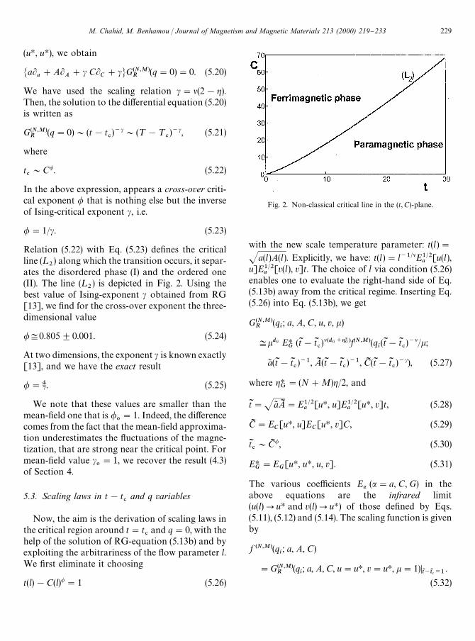
Fig. 2. Non-classical critical line in the (t, C)-plane.

(uH, uH), we obtain

MaLa#AL

A#c CL

C#cNG(N,M)

R(q"0)"0. (5.20)

We have used the scaling relation c"l(2!g).Then, the solution to the di!erential equation (5.20)is written as

G(N,M)R

(q"0)&(t!t#)~c&(¹!¹

#)~c, (5.21)

where

t#&C(. (5.22)

In the above expression, appears a cross-over criti-cal exponent / that is nothing else but the inverseof Ising-critical exponent c, i.e.

/"1/c. (5.23)

Relation (5.22) with Eq. (5.23) de"nes the criticalline (¸

2) along which the transition occurs, it separ-

ates the disordered phase (I) and the ordered one(II). The line (¸

2) is depicted in Fig. 2. Using the

best value of Ising-exponent c obtained from RG[13], we "nd for the cross-over exponent the three-dimensional value

/+0.805$0.001. (5.24)

At two dimensions, the exponent c is known exactly[13], and we have the exact result

/"47. (5.25)

We note that these values are smaller than themean-"eld one that is /

0"1. Indeed, the di!erence

comes from the fact that the mean-"eld approxima-tion underestimates the #uctuations of the magne-tization, that are strong near the critical point. Formean-"eld value c

0"1, we recover the result (4.3)

of Section 4.

5.3. Scaling laws in t!t#

and q variables

Now, the aim is the derivation of scaling laws inthe critical region around t"t

#and q"0, with the

help of the solution of RG-equation (5.13b) and byexploiting the arbitrariness of the #ow parameter l.We "rst eliminate it choosing

t(l)!C(l)("1 (5.26)

with the new scale temperature parameter: t(l )"

Ja(l)A(l). Explicitly, we have: t(l )"l~1@lE1@2a

[u(l),u]E1@2

a[v(l), v]t. The choice of l via condition (5.26)

enables one to evaluate the right-hand side of Eq.(5.13b) away from the critical regime. Inserting Eq.(5.26) into Eq. (5.13b), we get

G(N,M)R

(qi; a, A, C, u, v, k)

+kdG EHG

(tI!tI#)l(dG`gHG )f(N,M)(q

i(tI!tI

#)~l/k;

a8 (tI!tI#)~1, AI (tI!tI

#)~1, CI (tI!tI

#)~c), (5.27)

where gHG"(N#M)g/2, and

tI"Ja8 AI "E1@2a

[uH, u]E1@2a

[uH, v]t, (5.28)

CI "EC[uH, u]E

C[uH, v]C, (5.29)

tI#&CI (, (5.30)

EHG"E

G[uH, uH, u, v]. (5.31)

The various coe$cients Ea (a"a, C, G) in theabove equations are the infrared limit(u(l)PuH and v(l)PuH) of those de"ned by Eqs.(5.11), (5.12) and (5.14). The scaling function is givenby

f (N,M)(qi; a, A, C)

"G(N,M)R

(qi; a, A, C, u"uH, v"uH, k"1)D

tI~tI #/1.

(5.32)


Expression (5.27) merits two remarks. First, allexponents appearing in scaling law (5.27) dependonly on l and g, and the space dimension via d

G.

Second, the scaling function f (N,M) is independent ofu and v, therefore, it is universal. In fact, at thephysical "xed point, the scale factors Ea (a"a, C)absorb all non-universality, which comes from thedependence on the initial values of u and v remain-ing in the right-hand side of Eq. (5.27).

We can, also, derive the scaling laws in the wavevector q for the three propagators G(N,M)

Rwith

M#N"2. To do this, we choose the scale para-meter l as follows:

q/l"1. (5.33)

This choice of l via condition (5.33) allows us toobtain from Eq. (5.13b) the following scalinglaw:

G(N,M)R

(q; a, A, C, u, v, k)

"kdG EHG

qdG`gHGg(N,M)((tI!tI#)q~1@l;

a8 q~1@l, AI q~1@l, CI q~c@l), (5.34)

where the scaling function is given by

g(N,M)(t!t#, a, A, C)

"G(N,M)R

(a, A, C, u"uH, v"uH, k"1)Dq/1

.

(5.35)

In particular, in the limit of zero scattering-angle,that is when q goes to zero, the propagator behavesas

G(N,M)R

&q~(2~g) (N#M"2), (5.36)

where g is the usual Ising-critical exponent. Sucha behavior is similar to that usually encounteredwithin the framework of the para}ferromagnetictransition [5,12,13].

We note that when the various critical exponentstake their mean-"eld values, we recover the scalinglaws described in Section 4.

5.4. Small-scale behavior

By considering small scales compared to the cor-relation length m&(t!t

#)~l, we can obtain the

following behavior. Let i be a dilatation large fac-tor of wave vectors (q

iPiq

i), and choose the #ow

scale l to be equal to i. In the limit when both u(l)and v(l) go to uH, we "nd from Eq. (5.13b), at "xedt and C, the result

G(N,M)R

(iqi; a, A, C, u, v, k)

+kdG idG`gHG h(N,M)(qi/k,(tI!tI

#)i~1@l, a8 i~1@l,

AI i~1@l, CI i~c@l) (5.37)

with the scaling function

h(N,M)(qi; a, A, C)

"G(N,M)R

(qi; t!t

#, a, A, C, u"uH, v"uH, k"1).

(5.38)

At small scales, that is i~1;m, G(N,M)R

behaves as

G(N,M)R

&idG`gHG . (5.39)

Some non-universal factor is ignored in Eq. (5.39).In the mean-"eld limit, we recover the classicalbehavior.

6. Concluding remarks

We recall that this work was concerned witha theoretical investigation of the critical propertiesof the para}ferrimagnetic transition, arising instrongly coupled paramagnetic systems. To takeinto account the strong #uctuations of magneti-zation around the critical point, we have elaborateda renormalization theory applied to a "eld modeldescribing such a transition. We have "rst shownthat the associated "eld theory is renormalizable atany order of the perturbation series in the couplingconstants, up to critical dimension d

#"4, and that,

the necessary counterterms to remove short-rangedivergences are similar to those of the usual theory.Second, using RG-techniques, we have obtained allthese critical properties, with respect to the relevantparameters, namely, the wave vector, the temper-ature and the coupling between the two-sublatticesof the system under consideration. In particular, wehave derived the exact equation for the critical line,along which the system undergoes a phase


transition, in the (t,C)-plane. In this equation, ap-pears a cross-over critical exponent which is foundto be the inverse of Ising-critical exponent c.

For the physical "xed point, appear only thosecritical exponents relative to Ising-like magneticsystems. In this sense, we can say that the secondorder para}ferrimagnetic transition belongs to thesame universality class as the traditional para}fer-romagnetic one.

We note that the continuous model we con-sidered is convenient for 1

2-spin systems, and it was

su$cient to consider only those pure quartic termsin both "elds u and t. However, in the case of spin1-systems, some additional biquadratic exchangeinteraction term wu2t2 may be taken into accountfor the consistence of the theory. Physically speak-ing, this extra interaction is associated with thecubic anisotropy [25]. Then, the natural questionto ask is how the critical behavior of the systemwould be a!ected by the presence of this interac-tion. The answer to such a question is in progress[26].

We "nish these concluding remarks by askinga question about the possible appearance of quarticcouplings like u

1u3t and u

2ut3 in the free energy.

To our opinion, these self-interaction terms do nothave a real physical sense.

Acknowledgements

We are very much indebted to our referee for hispertinent remarks and suggestions.

Appendix A

The purpose of this appendix is to show howa continuous model of free energy (2.1) can beemerged from a discrete 1

2-spin Hamiltonian, de-

scribing the para}ferrimagnetic transition of twostrongly coupled Curie}Weiss paramagnetic sub-systems. To this end, consider two coupled sublatti-ces X

1and X

2of Euclidean dimension d. On each

site i3X1

and i@3X2, we attribute two variables

Si"$1 and S

i{"$1, respectively. We denote by

J1

and J2

the exchange integrals inside X1

and X2,

and by J12

that between X1

and X2. To a given

con"guration of spins, we associate the discreteHamiltonian

IH"!+ij

[J1]ijSiSj!+

i{j{

[J2]i{j{

Si{Sj{

!+ij{

[J12

]ij{

SiSj{!+

i

hiSi!+

i{

hi{Si{

(A.1)

We have [J1]ij"J

1, [J

2]i{j{

"J2

and[J

12]ij{"J

12, for nearest-neighbors sites, and 0,

otherwise. We will suppose that J1'0 and J

2'0

(ferromagnetic couplings), and J12

(0 (antifer-romagnetic coupling). The variables h

iand

hi{

stand for external magnetic "elds applied to sitesi3X

1and i@3X

2, respectively.

The starting point is the partition function or thegenerating functional that is given by

Z[hI ]" +MSI i/B1N

expM!bIHN

" +MSI i/B1N

expG+ij

KijSIiSIj#+

i

hIiSIiH. (A.2)

Here, b"(kB¹)~1, where ¹ is the absolute temper-

ature and kB

the Boltzmann constant. Summationin Eq. (A.2) is performed over all 2@X1 @]2@X2 @ pos-sible con"gurations, where DXa D is the number ofsites inside the sublattice a. We have rede"ned theexchange integrals to get dimensionless ones, ac-cording to

Kij"G

b[J1]ij, (i, j)3X

1]X

1,

b[J2]i{j{

, (i@, j@)3X2]X

2,

b[J12

]ij{

, (i, j@)3X1]X

2.

(A.3)

In de"nition (A.2), the notations SIi

and hIi

are asfollows:

SIi"G

Si, i3X

1,

Si{, i@3X

2

(A.4)

and

hIi"G

bhi, i3X

1,

bhi{, i@3X

2.

(A.5)

which is the reduced magnetic "eld.Now, the passage from discrete to continuous

formulation can be made through the standard


Gaussian integral representation

P`=

~=

N<i/1

dxiexpA!

1

4+ij

xiD

ijxj#+

i

SixiB

"constant]expA+ij

SiD~1

ijSjB, (A.6)

where D"(Dij) is any symmetric positive de"nite

squared matrix. In our case, D is nothing else butthe inverse of the coupling constant matrix K de-"ned above. Thanks to this representation and per-forming summation over the spin variables SI

i, the

partition function de"ned by Eq. (A.2) can be re-written as a functional integral

Z[hI ]"Z0P

`=

~=C<i|X

d/iD expG!

1

4+ij

(/i!hI

i)

][K~1]ij(/

j!hI

j)#+

i

A(/i)H, (A.7)

where Z0"Z[hI "0] is the normalization con-

stant, and X"X1XX

2. We have

A(/i)"ln(cosh /

i). (A.8a)

The "eld /iis de"ned by

/i"G

ui, i3X

1,

ti{, i@3X

2.

(A.8b)

The integral (A.7) can be calculated using thesteepest descent method [27], which gives, atlowest order, the mean-"eld theory. We "rst per-form the translation

/i"X

i#/I

i, (A.9)

where Xi

is the con"guration giving the lowestpotential energy, and /I

iis the #uctuation around

the saddle point (classical solution). The methodconsists in making expansion in powers of /I

i. Then,

we have

!bIHM/N"!bIHMXN!1

4/I K~1/I

#

1

2+i

/I 2iAA(X

i)#2. (A.10)

Then, the generating functional becomes

Z[hI ]"Const.eW0 *hI +P`=

~=C<i|X

d/IiD

]expG!1

4+ij

/Ii[K~1]

ij/I

j

#

1

2+i

/I 2iAA(X

i)#2H. (A.11)

The "rst approximation to the Helmoltz freeenergy=[hI ]"ln Z[hI ] is =

0[hI ], such that

=0[hI ]"!1

4+ij

(Xi!hI

i)[K~1]

ij(X

j!hI

j)

#+i

A(Xi)DXi/Xi *hI +

. (A.12)

Now, consider the magnetization m8i

relative toa site i of the lattice X"X

1XX

2, and denote

m8i"G

Mi, i3X

1,

mi{, i@3X

2

(A.13)

that is given by the "rst functional derivative of thefree energy, with respect to the magnetic "eld hI

i

m8i"

d=[hI ]dhI

i

. (A.14)

To the lowest order, the magnetization reads

m8i"

d=0[hI ]

dhIi

"

1

2+j

[K~1]ij(X

j!hI

j)

"A@(Xi)DXi/Xi *hI +

. (A.15)

It will be more convenient to discuss the problemin terms of the magnetization m8 and the corre-sponding thermodynamic potential or propergenerating functional C

0[m8 ], which is the Legendre

transform of the Helmoltz free energy

C0[m8 ]#=

0[hI ]"+

i|XhIim8

i, (A.16)

in which the hIis are the solution of Eq. (A.15). This

yields the tree approximation expression of thethermodynamic potential

C0[m8 ]"!+

ij

m8iK

ijm8

j#+

i

B(m8i) (A.17)


with

B(m8i)"[X

im8

i!A(X

i)]

m8 i/A{(Xi ). (A.18)

More explicitly, for Ising model, we obtain

B(m8i)"A

1#m8i

2 B lnA1#m8

i2 B

#A1!m8

i2 B lnA

1!m8i

2 B. (A.19)

The thermodynamic potential (A.17) with Eq.(A.19) constitutes the well-known Bragg}Williamsfree energy [4]. The second term on the right-handside of Eq. (A.19) represents the entropy reduced bythe !k

Bfactor.

In the case of a uniform magnetic "eld, that is forhIi"hI ,H, magnetizations are independent of

sites, and we write

m8 "GM for X

1m for X

2

(A.20)

Thus, Eq. (A.16) with Eq. (A.18) yields the desiredfree energy F[m,M]"k

B¹MC

0[m, M]!

H(m#M)N, or explicitly

F[m,M]

kB¹

"

a

2m2#

A

2M2!CmM#

u

4m4#

v

4M4

!H(m#M) (A.21)

with

a"1!z1J1

kB¹

, A"1!z2J2

kB¹

, C"

z12

J12

kB¹

(A.22)

and

u"v"13. (A.23)

Here z1, z

2and z

12are, respectively, the numbers

of nearest neighbors inside X1

and X2, and between

X1

and X2.

The free energy (A.21) de"nes the Landau con-tinuous model, which has been used in the previous

works [1,9,10], to describe the super-weak ferrimag-netism arising from 1

2-spin systems.

References

[1] K.U. Neumann, J. Crangle, K.R.A. Ziebeck, J. Magn.Magn. Mater. 127 (1993) 47.

[2] G. Chouteau, R. Yazami, Private communication.[3] J.C. ToleH dano, The Landau Theory of Phase Transitions,

World Scienti"c, Singapore, 1987.[4] H.E. Stanley, Introduction to Phase Transitions and Criti-

cal Phenomena, Clarendon Press, Oxford, 1971.[5] D. Amit, Field Theory, The Renormalization Group and

Critical Phenomena, McGraw-Hill, New York, 1978.[6] K.U. Neumann, S. Lipinski, K.R.A. Ziebeck, Solid State

Commun. 91 (1994) 443.[7] W. Pauli, Z. Physik 41 (1927) 81.[8] C. Kittel, Physique de l'Etat solide, Dunod and Bordas,

Paris, 1983.[9] B. El Houari, M. Benhamou, M. El Ha"di, G. Chouteau,

J. Magn. Magn. Mater. 166 (1997) 97.[10] B. El Houari, M. Benhamou, J. Magn. Magn. Mater. 172

(1997) 259.[11] J.C. Collins, Renormalization, Cambridge University

Press, Cambridge, 1985.[12] J. Zinn-Justin, Quantum Field Theory and Critical Phe-

nomena, Clarendon Press, Oxford, 1989.[13] C. Itzykson, J.M. Drou!e, Statistical Field Theory, Vol. 1,

Cambridge University Press, Cambridge, 1989.[14] P. Weiss, R. Forrer, Ann. Phys. Paris 5 (1926) 153.[15] C. Chahine, Thermodynamique Statistique, Dunod and

Bordas, Paris, 1986.[16] A. Rougier, These d'UniversiteH , Bordeaux, France, 1995.[17] C. Itzykson, J.B. Zuber, Quantum Field Theory,

McGraw-Hill, New York, 1980.[18] N. Nakanishi, Prog. Theoret. Phys. (Suppl.) 18 (1961) 1.[19] M.C. Bergere, Y.M.P. Lam, J. Math. Phys. 17 (1975) 227.[20] N. Nakanishi, Graph Theory and Feynmann Integrals,

Gordon and Breach, New York, 1970.[21] I.T. Todorov, Analytic Properties of Feynmann Diagrams

in Quantum Field Theory, Pergamon Press, New York,1971.

[22] K. Hepp, Commun. Math. Phys. 2 (1966) 301.[23] G. 't Hooft, M. Veltman, Nucl. Phys. B 44 (1972) 189.[24] G. 't Hooft, Nucl. Phys. B 61 (1973) 455.[25] D.R. Nelson, J.M. Kosterlitz, M.E. Fisher, Phys. Rev. Lett.

33 (1974) 813.[26] M. Chahid, M. Benhamou, in preparation.[27] E. BreH zin, J.C. Le Guillou, J. Zinn-Justin, in: C. Domb,

M.S. Green (Eds.), Phase Transition and Critical Phe-nomena, Vol. 6, Academic Press, NY, 1976.


field theoretical approach to the paramagnetic-ferrimagnetic transition in strongly coupled...

Documents