fall 20101 csc 446/546 part 10: estimation of absolute performance
TRANSCRIPT
Fall
20
10
1
CSC 446/546
Part 10: Estimation of Absolute Performance
Fall
20
10
1
CSC 446/546
Agenda
1. Type of Simulation w.r.t. Output Analysis
2. Stochastic Nature of Output Data
3. Absolute Measures
4. Output Analysis for Terminating Simulation
5. Output Analysis for Steady-State Simulation
Fall
20
10
1
CSC 446/546 3
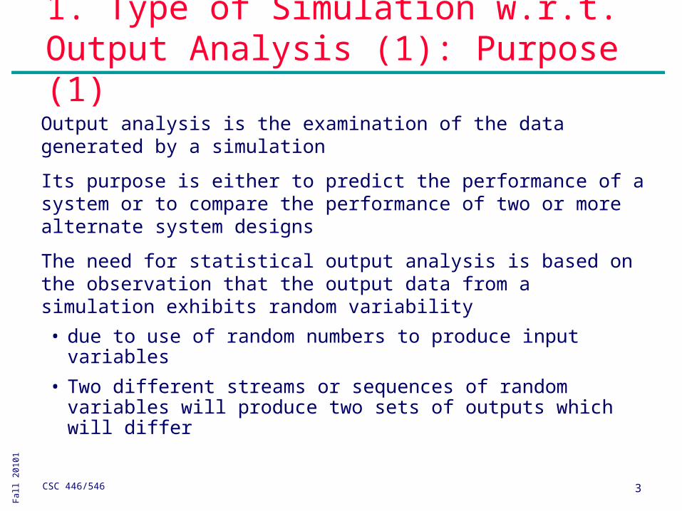
1. Type of Simulation w.r.t. Output Analysis (1): Purpose (1)Output analysis is the examination of the data generated by a simulation
Its purpose is either to predict the performance of a system or to compare the performance of two or more alternate system designs
The need for statistical output analysis is based on the observation that the output data from a simulation exhibits random variability
• due to use of random numbers to produce input variables
• Two different streams or sequences of random variables will produce two sets of outputs which will differ
Fall
20
10
1
CSC 446/546 4
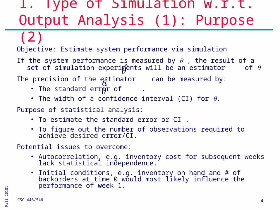
1. Type of Simulation w.r.t. Output Analysis (1): Purpose (2)Objective: Estimate system performance via simulation
If the system performance is measured by , the result of a set of simulation experiments will be an estimator of
The precision of the estimator can be measured by:• The standard error of .• The width of a confidence interval (CI) for .
Purpose of statistical analysis:• To estimate the standard error or CI .• To figure out the number of observations required to achieve
desired error/CI.
Potential issues to overcome: • Autocorrelation, e.g. inventory cost for subsequent weeks lack
statistical independence.• Initial conditions, e.g. inventory on hand and # of backorders at
time 0 would most likely influence the performance of week 1.
Fall
20
10
1
CSC 446/546 5
1. Type of Simulation w.r.t. Output Analysis (1): Purpose (3)Distinguish the two types of simulation: transient vs. steady state.
Illustrate the inherent variability in a stochastic discrete-event simulation.
Cover the statistical estimation of performance measures.
Discusses the analysis of transient simulations.
Discusses the analysis of steady-state simulations.
Fall
20
10
1
CSC 446/546 6
1. Type of Simulation w.r.t. Output Analysis (2)Terminating verses non-terminating simulations
Terminating simulation:
• Runs for some duration of time TE, where E is a specified event that stops the simulation.
• Starts at time 0 under well-specified initial conditions.
• Ends at the stopping time TE.
• Bank example: Opens at 8:30 am (time 0) with no customers present and 8 of the 11 teller working (initial conditions), and closes at 4:30 pm (Time TE = 480 minutes).
• The simulation analyst chooses to consider it a terminating system because the object of interest is one day’s operation.
Fall
20
10
1
CSC 446/546 7
1. Type of Simulation w.r.t. Output Analysis (3)Non-terminating simulation:
• Runs continuously, or at least over a very long period of time.
• Examples: assembly lines that shut down infrequently, telephone systems, hospital emergency rooms.
• Initial conditions defined by the analyst.
• Runs for some analyst-specified period of time TE.
• Study the steady-state (long-run) properties of the system, properties that are not influenced by the initial conditions of the model.
Whether a simulation is considered to be terminating or non-terminating depends on both
• The objectives of the simulation study and
• The nature of the system.
Fall
20
10
1
CSC 446/546 8
2. Stochastic Nature of Output Data (1)Model output consist of one or more random variables because the model is an input-output transformation and the input variables are r.v.’s.
M/G/1 queueing example:
• Poisson arrival rate = 0.1 per minute; service time ~ N(= 9.5, =1.75).
• System performance: long-run mean queue length, LQ(t).
• Suppose we run a single simulation for a total of 5,000 minutes– Divide the time interval [0, 5000) into 5 equal
subintervals of 1000 minutes.– Average number of customers in queue from time (j-
1)1000 to j(1000) is Yj .
Fall
20
10
1
CSC 446/546 9
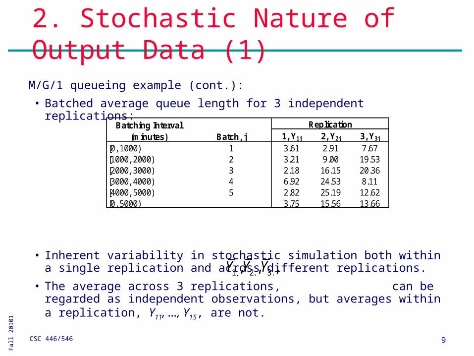
2. Stochastic Nature of Output Data (1)M/G/1 queueing example (cont.):
• Batched average queue length for 3 independent replications:
• Inherent variability in stochastic simulation both within a single replication and across different replications.
• The average across 3 replications, can be regarded as independent observations, but averages within a replication, Y11, …, Y15, are not.
1, Y1j 2, Y2j 3, Y3j
[0, 1000) 1 3.61 2.91 7.67[1000, 2000) 2 3.21 9.00 19.53[2000, 3000) 3 2.18 16.15 20.36[3000, 4000) 4 6.92 24.53 8.11[4000, 5000) 5 2.82 25.19 12.62[0, 5000) 3.75 15.56 13.66
ReplicationBatching Interval (minutes) Batch, j
,,, .3.2.1 YYY
Fall
20
10
1
CSC 446/546 10
3. Absolute Measures (1)
Consider the estimation of a performance parameter, (or ), of a simulated system.
It is desired to have a “point estimate” and an “interval estimate” of (or )• In many cases, there is an obvious or natural choice
candidate for a point estimator. Sample mean is such an example
• Interval estimates expand on “point estimates” by incorporating the uncertainty of point estimates– Different samples from different intervals may have
different means– An interval estimate quantifies this uncertainty by
computing lower and upper values with a given level of confidence (i.e., probability)
Fall
20
10
1
CSC 446/546 11
3. Absolute Measures (2)
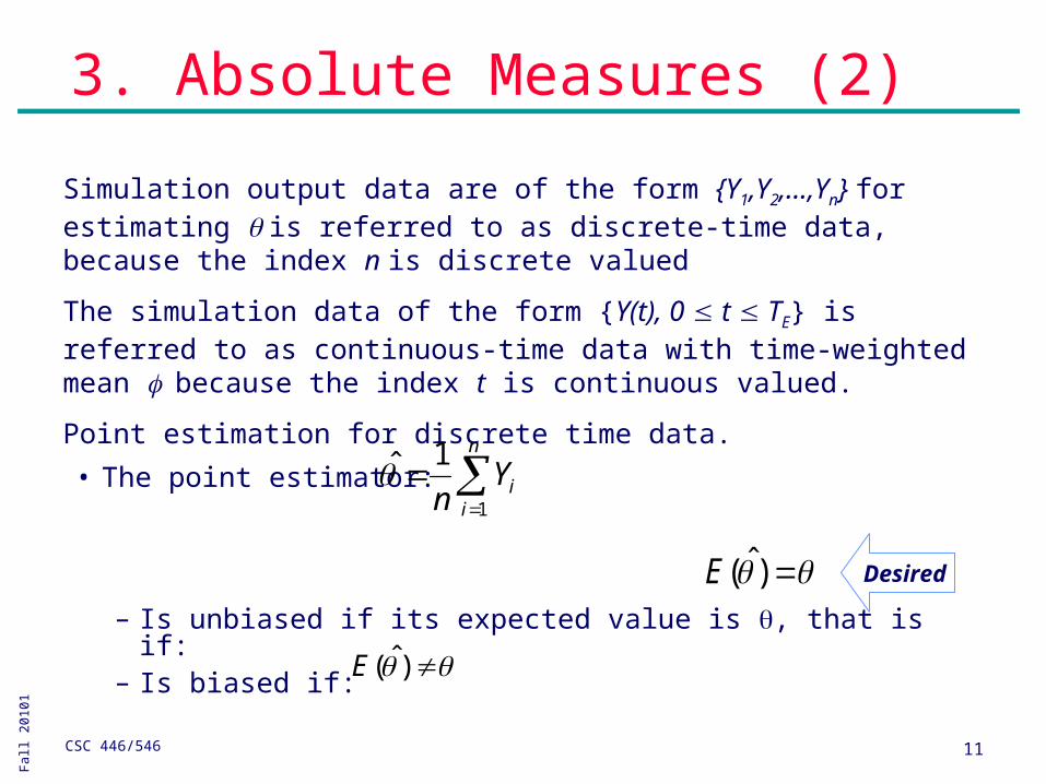
Simulation output data are of the form {Y1,Y2,…,Yn} for estimating is referred to as discrete-time data, because the index n is discrete valued
The simulation data of the form {Y(t), 0 t TE} is referred to as continuous-time data with time-weighted mean because the index t is continuous valued.
Point estimation for discrete time data.
• The point estimator:
– Is unbiased if its expected value is , that is if:– Is biased if:
)ˆ(E Desired
)ˆ(E
n
iiYn 1
1
Fall
20
10
1
CSC 446/546 12
3. Absolute Measures (3): Point Estimator (1)
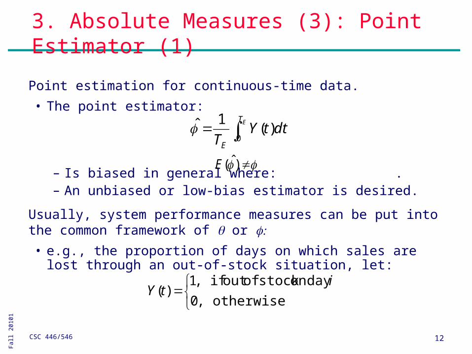
Point estimation for continuous-time data.
• The point estimator:
– Is biased in general where: .– An unbiased or low-bias estimator is desired.
Usually, system performance measures can be put into the common framework of or • e.g., the proportion of days on which sales are lost through
an out-of-stock situation, let:
)ˆ(E
ET
E
dttYT 0
)(1
otherwise ,0
day on stock ofout if ,1)(
itY
Fall
20
10
1
CSC 446/546 13
3. Absolute Measures (3): Point Estimator (2)
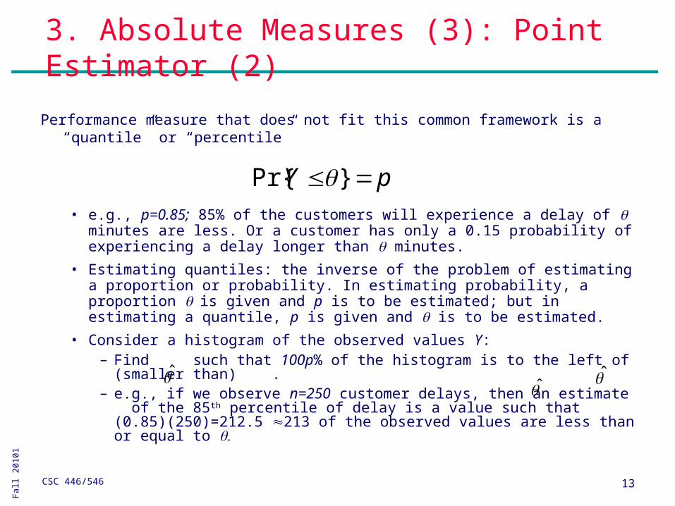
Performance measure that does not fit this common framework is a “quantile” or “percentile”
• e.g., p=0.85; 85% of the customers will experience a delay of minutes are less. Or a customer has only a 0.15 probability of experiencing a delay longer than minutes.
• Estimating quantiles: the inverse of the problem of estimating a proportion or probability. In estimating probability, a proportion is given and p is to be estimated; but in estimating a quantile, p is given and is to be estimated.
• Consider a histogram of the observed values Y:– Find such that 100p% of the histogram is to the left of (smaller
than) .– e.g., if we observe n=250 customer delays, then an estimate
of the 85th percentile of delay is a value such that (0.85)(250)=212.5 213 of the observed values are less than or equal to
pY }Pr{
Fall
20
10
1
CSC 446/546 14
3. Absolute Measures (3): Confidence-Interval Estimation (1)
To understand confidence intervals fully, it is important to distinguish between measures of error, and measures of risk
• contrast the confidence interval with a prediction interval (another useful output-analysis tool).
• Both confidence and prediction intervals are based on premise that the data being produced by the simulation is well represented by a probability model
Fall
20
10
1
CSC 446/546 15
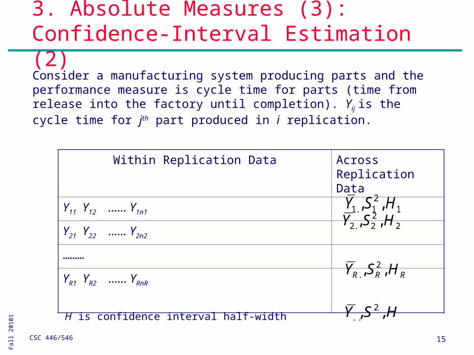
3. Absolute Measures (3): Confidence-Interval Estimation (2)Consider a manufacturing system producing parts and the performance measure is cycle time for parts (time from release into the factory until completion). Yij is the cycle time for jth part produced in i replication.
Within Replication Data Across Replication Data
Y11 Y12 …… Y1n1
Y21 Y22 …… Y2n2
………
YR1 YR2 …… YRnR
12
1.1 ,, HSY2
22.2 ,, HSY
RRR HSY ,, 2.
HSY ,, 2.. H is confidence interval half-width
Fall
20
10
1
CSC 446/546 16
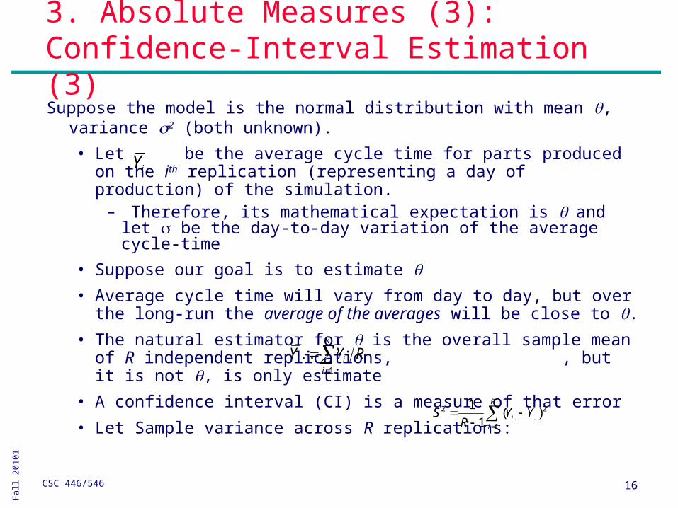
3. Absolute Measures (3): Confidence-Interval Estimation (3)Suppose the model is the normal distribution with mean ,
variance 2 (both unknown).
• Let be the average cycle time for parts produced on the ith replication (representing a day of production) of the simulation.
– Therefore, its mathematical expectation is and let be the day-to-day variation of the average cycle-time
• Suppose our goal is to estimate • Average cycle time will vary from day to day, but over the
long-run the average of the averages will be close to .• The natural estimator for is the overall sample mean of R
independent replications, , but it is not , is only estimate
• A confidence interval (CI) is a measure of that error
• Let Sample variance across R replications:
R
ii RYY
1...
R
ii YY
RS
1
2...
2 )(1
1
.iY
Fall
20
10
1
CSC 446/546 17
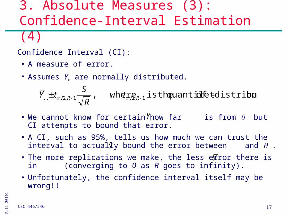
3. Absolute Measures (3): Confidence-Interval Estimation (4)
Confidence Interval (CI):
• A measure of error.
• Assumes Yi. are normally distributed.
• We cannot know for certain how far is from but CI attempts to bound that error.
• A CI, such as 95%, tells us how much we can trust the interval to actually bound the error between and .
• The more replications we make, the less error there is in (converging to 0 as R goes to infinity).
• Unfortunately, the confidence interval itself may be wrong!!
ondistributi- tof quantile theis where, 1,2/1,2/.. RR tR
StY
..Y
..Y..Y
Fall
20
10
1
CSC 446/546 18
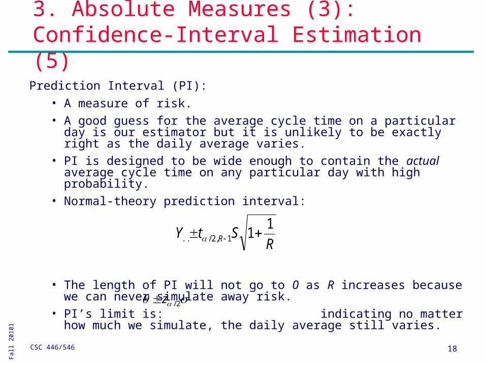
3. Absolute Measures (3): Confidence-Interval Estimation (5)
Prediction Interval (PI):• A measure of risk.• A good guess for the average cycle time on a particular day
is our estimator but it is unlikely to be exactly right as the daily average varies.
• PI is designed to be wide enough to contain the actual average cycle time on any particular day with high probability.
• Normal-theory prediction interval:
• The length of PI will not go to 0 as R increases because we can never simulate away risk.
• PI’s limit is: indicating no matter how much we simulate, the daily average still varies.
RStY R
111,2/..
2/z
Fall
20
10
1
CSC 446/546 19
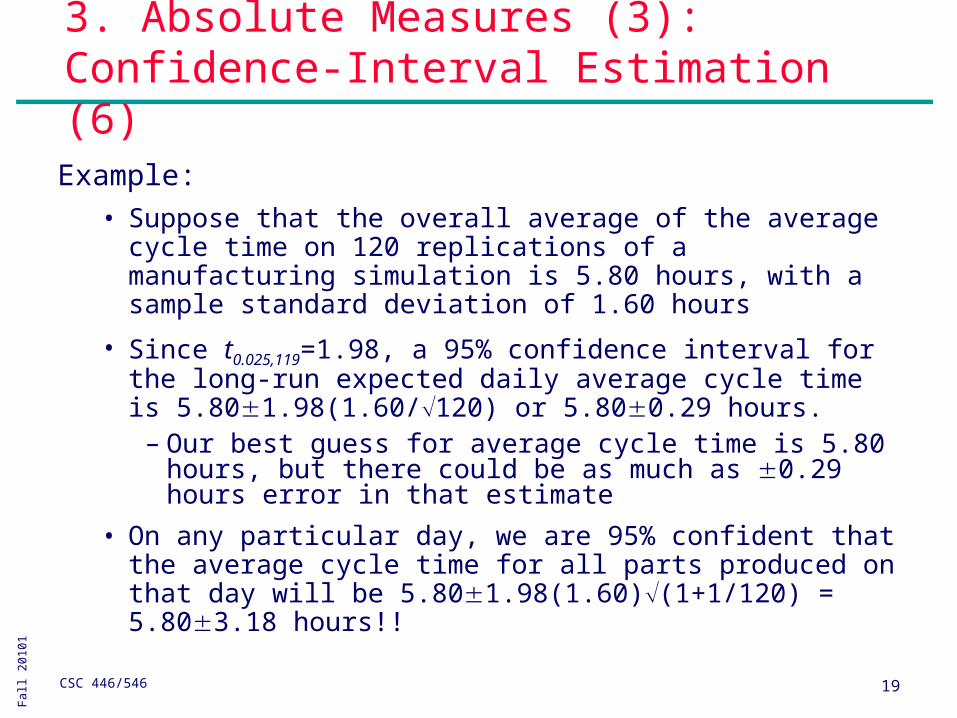
3. Absolute Measures (3): Confidence-Interval Estimation (6)
Example:• Suppose that the overall average of the average cycle
time on 120 replications of a manufacturing simulation is 5.80 hours, with a sample standard deviation of 1.60 hours
• Since t0.025,119=1.98, a 95% confidence interval for the long-run expected daily average cycle time is 5.801.98(1.60/120) or 5.800.29 hours.– Our best guess for average cycle time is 5.80
hours, but there could be as much as 0.29 hours error in that estimate
• On any particular day, we are 95% confident that the average cycle time for all parts produced on that day will be 5.801.98(1.60)(1+1/120) = 5.803.18 hours!!
Fall
20
10
1
CSC 446/546 20
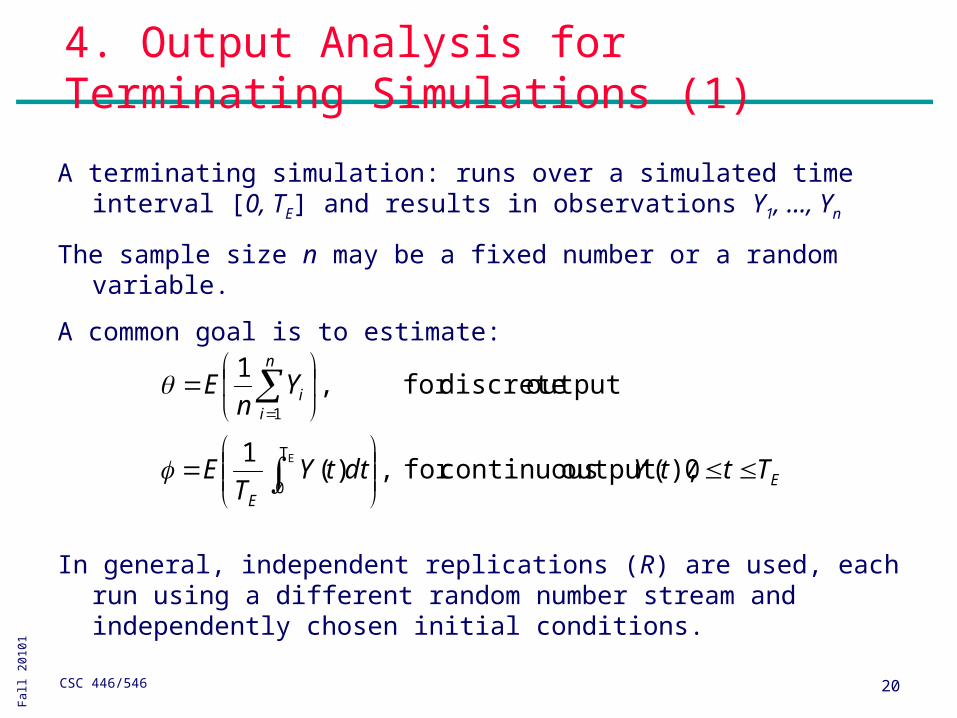
4. Output Analysis for Terminating Simulations (1)
A terminating simulation: runs over a simulated time interval [0, TE] and results in observations Y1, …, Yn
The sample size n may be a fixed number or a random variable.
A common goal is to estimate:
In general, independent replications (R) are used, each run using a different random number stream and independently chosen initial conditions.
EE
n
ii
TttYdttYT
E
Yn
E
0),(output continuousfor ,)(1
output discretefor ,1
ET
0
1
Fall
20
10
1
CSC 446/546 21
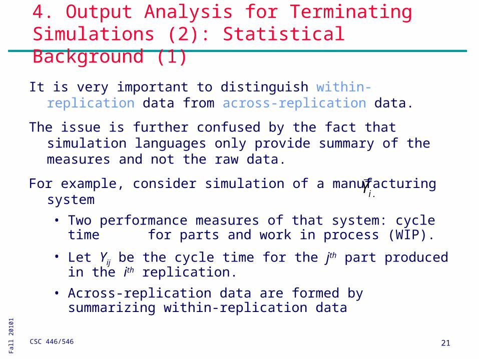
4. Output Analysis for Terminating Simulations (2): Statistical Background (1)
It is very important to distinguish within-replication data from across-replication data.
The issue is further confused by the fact that simulation languages only provide summary of the measures and not the raw data.
For example, consider simulation of a manufacturing system
• Two performance measures of that system: cycle time for parts and work in process (WIP).
• Let Yij be the cycle time for the jth part produced in the ith replication.
• Across-replication data are formed by summarizing within-replication data
.iY
Fall
20
10
1
CSC 446/546 22
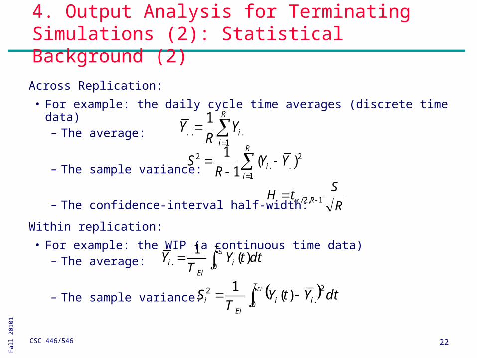
4. Output Analysis for Terminating Simulations (2): Statistical Background (2)
Across Replication:
• For example: the daily cycle time averages (discrete time data)– The average:
– The sample variance:
– The confidence-interval half-width:
Within replication:
• For example: the WIP (a continuous time data)– The average:
– The sample variance:
R
iiYR
Y1
...
1
R
ii YY
RS
1
2...
2 )(1
1
R
StH R 1,2/
EiT
iEi
i dttYT
Y0. )(
1
EiT
iiEi
i dtYtYT
S0
2
.2 )(
1
Fall
20
10
1
CSC 446/546 23
4. Output Analysis for Terminating Simulations (2): Statistical Background (3)
Overall sample average, , and the interval replication sample averages, , are always unbiased estimators of the expected daily average cycle time or daily average WIP.
Across-replication data are independent (different random numbers) and identically distributed (same model), but within-replication data do not have these properties.
..Y .iY
Fall
20
10
1
CSC 446/546 24
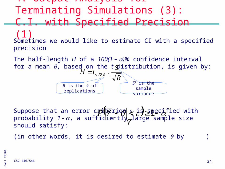
4. Output Analysis for Terminating Simulations (3): C.I. with Specified Precision (1)Sometimes we would like to estimate CI with a specified precision
The half-length H of a 100(1 – )% confidence interval for a mean , based on the t distribution, is given by:
Suppose that an error criterion is specified with probability 1 - , a sufficiently large sample size should satisfy:
(in other words, it is desired to estimate by )
R
StH R 1,2/
R is the # of replications
S2 is the sample variance
1..YP..Y
Fall
20
10
1
CSC 446/546 25
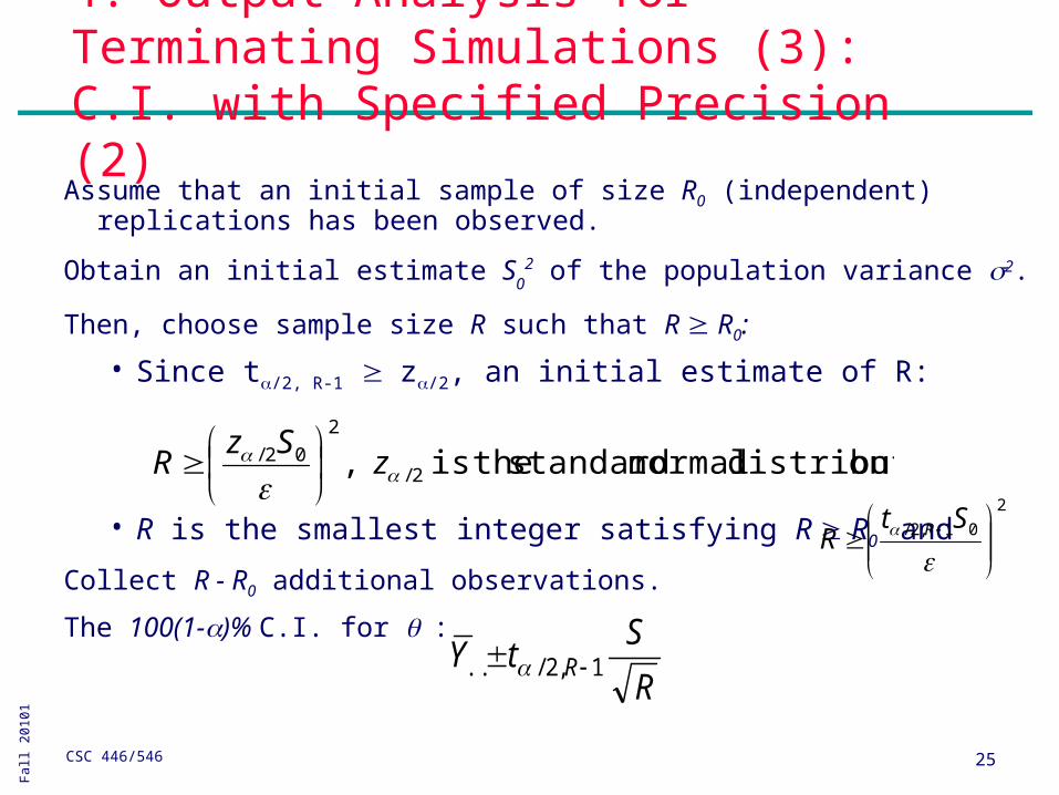
4. Output Analysis for Terminating Simulations (3): C.I. with Specified Precision (2)Assume that an initial sample of size R0 (independent)
replications has been observed.
Obtain an initial estimate S0
2 of the population variance 2.
Then, choose sample size R such that R R0:
• Since t/2, R-1 z/2, an initial estimate of R:
• R is the smallest integer satisfying R R0 and
Collect R - R0 additional observations.
The 100(1-)% C.I. for :
on.distributi normal standard theis , 2/
2
02/
z
SzR
2
01,2/
St
R R
R
StY R 1,2/..
Fall
20
10
1
CSC 446/546 26
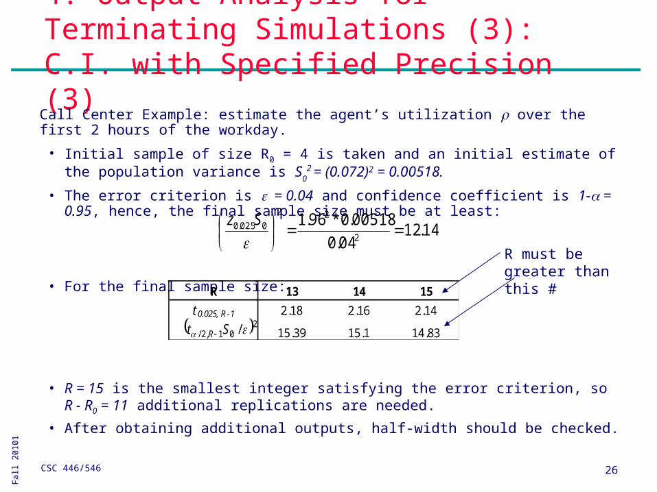
4. Output Analysis for Terminating Simulations (3): C.I. with Specified Precision (3)Call Center Example: estimate the agent’s utilization over the first 2 hours of the workday.
• Initial sample of size R0 = 4 is taken and an initial estimate of the population variance is S
02 = (0.072)2 = 0.00518.
• The error criterion is = 0.04 and confidence coefficient is 1- = 0.95, hence, the final sample size must be at least:
• For the final sample size:
• R = 15 is the smallest integer satisfying the error criterion, so R - R0 = 11 additional replications are needed.
• After obtaining additional outputs, half-width should be checked.
14.1204.0
00518.0*96.12
22
0025.0
Sz
R 13 14 15
t 0.025, R-1 2.18 2.16 2.14
15.39 15.1 14.83 201,2/ / St R
R must be greater thanthis #
Fall
20
10
1
CSC 446/546 27
4. Output Analysis for Terminating Simulations (4): Quantiles (1)
To present the interval estimator for quantiles,
• it is helpful to look at the interval estimator for a mean in the special case when mean represents a proportion or probability, p
In this book, a proportion or probability is treated as a special case of a mean.
Fall
20
10
1
CSC 446/546 28
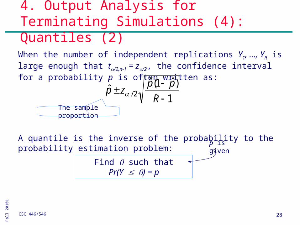
4. Output Analysis for Terminating Simulations (4): Quantiles (2)
When the number of independent replications Y1, …, YR is large enough that t/2,n-1 = z/2, the confidence interval for a probability p is often written as:
A quantile is the inverse of the probability to the probability estimation problem:
1
)ˆ1(ˆˆ 2/
R
ppzp
Find such that Pr(Y) = p
p is given
The sample proportion
Fall
20
10
1
CSC 446/546 29
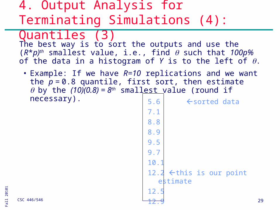
4. Output Analysis for Terminating Simulations (4): Quantiles (3)The best way is to sort the outputs and use the (R*p)th smallest value, i.e., find such that 100p% of the data in a histogram of Y is to the left of .• Example: If we have R=10 replications and we want the p
= 0.8 quantile, first sort, then estimate by the (10)(0.8) = 8th smallest value (round if necessary).
5.6sorted data
7.1
8.8
8.9
9.5
9.7
10.1
12.2 this is our point estimate
12.5
12.9
Fall
20
10
1
CSC 446/546 30
4. Output Analysis for Terminating Simulations (4): Quantiles (4)
1
)1(
1
)1( where
2/
2/
R
ppzpp
R
ppzpp
u
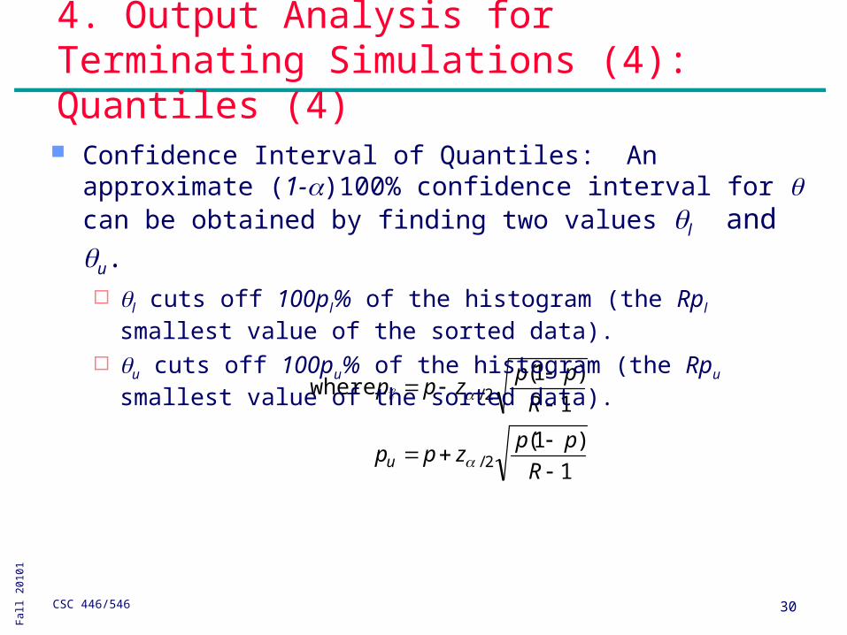
Confidence Interval of Quantiles: An approximate (1-)100% confidence interval for can be obtained by finding two values l and u. l cuts off 100pl% of the histogram (the Rpl smallest value of the
sorted data). u cuts off 100pu% of the histogram (the Rpu smallest value of the
sorted data).
Fall
20
10
1
CSC 446/546 31
4. Output Analysis for Terminating Simulations (4): Quantiles (5)
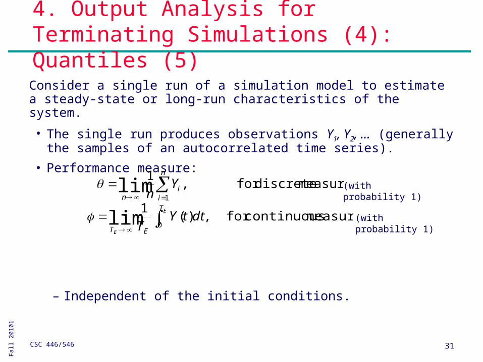
Consider a single run of a simulation model to estimate a steady-state or long-run characteristics of the system.
• The single run produces observations Y1, Y2, ... (generally the samples of an autocorrelated time series).
• Performance measure:
– Independent of the initial conditions.
measure discretefor ,1
1lim
n
ii
n
Yn
measure continuousfor ,)(1
0lim
E
E
T
ET
dttYT
(with probability 1)
(with probability 1)
Fall
20
10
1
CSC 446/546 32
5. Output Analysis for Steady-State Simulation (1)
The sample size is a design choice, with several considerations in mind:
• Any bias in the point estimator that is due to artificial or arbitrary initial conditions (bias can be severe if run length is too short).
• Desired precision of the point estimator.
• Budget constraints on computer resources.
Notation: the estimation of from a discrete-time output process.
• One replication (or run), the output data: Y1, Y2, Y3, …
• With several replications, the output data for replication r: Yr1, Yr2, Yr3, …
Fall
20
10
1
CSC 446/546 33
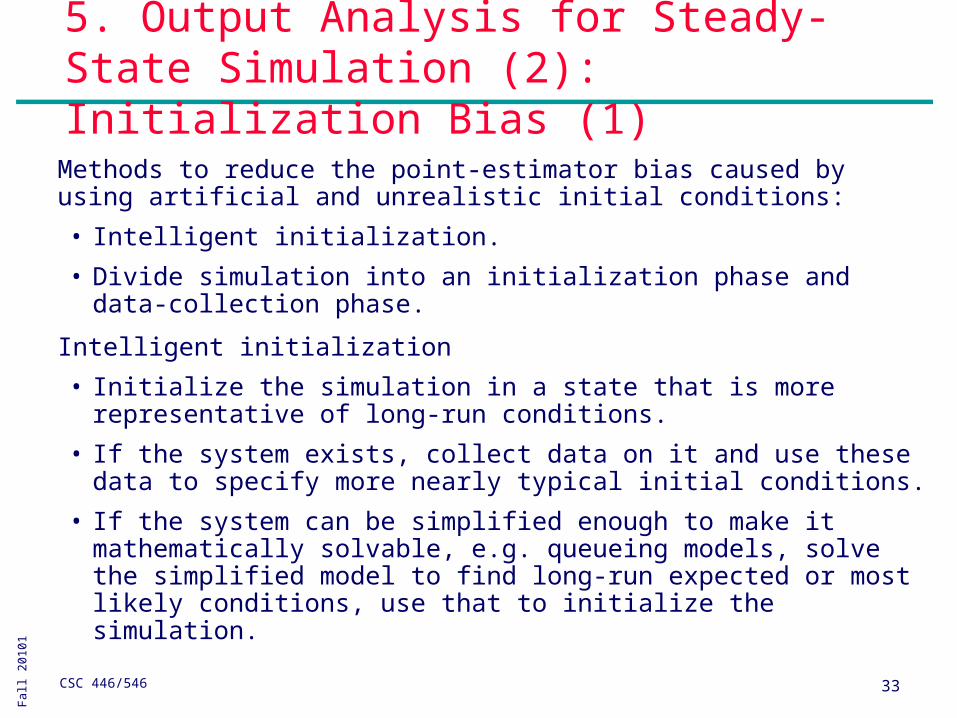
5. Output Analysis for Steady-State Simulation (2): Initialization Bias (1)
Methods to reduce the point-estimator bias caused by using artificial and unrealistic initial conditions:
• Intelligent initialization.
• Divide simulation into an initialization phase and data-collection phase.
Intelligent initialization
• Initialize the simulation in a state that is more representative of long-run conditions.
• If the system exists, collect data on it and use these data to specify more nearly typical initial conditions.
• If the system can be simplified enough to make it mathematically solvable, e.g. queueing models, solve the simplified model to find long-run expected or most likely conditions, use that to initialize the simulation.
Fall
20
10
1
CSC 446/546 34
5. Output Analysis for Steady-State Simulation (2): Initialization Bias (2)
Divide each simulation into two phases:
• An initialization phase, from time 0 to time T0.
• A data-collection phase, from T0 to the stopping time T0+TE.
• The choice of T0 is important:
– After T0, system should be more nearly representative of steady-state behavior.
• System has reached steady state: the probability distribution of the system state is close to the steady-state probability distribution (bias of response variable is negligible).
Fall
20
10
1
CSC 446/546 35
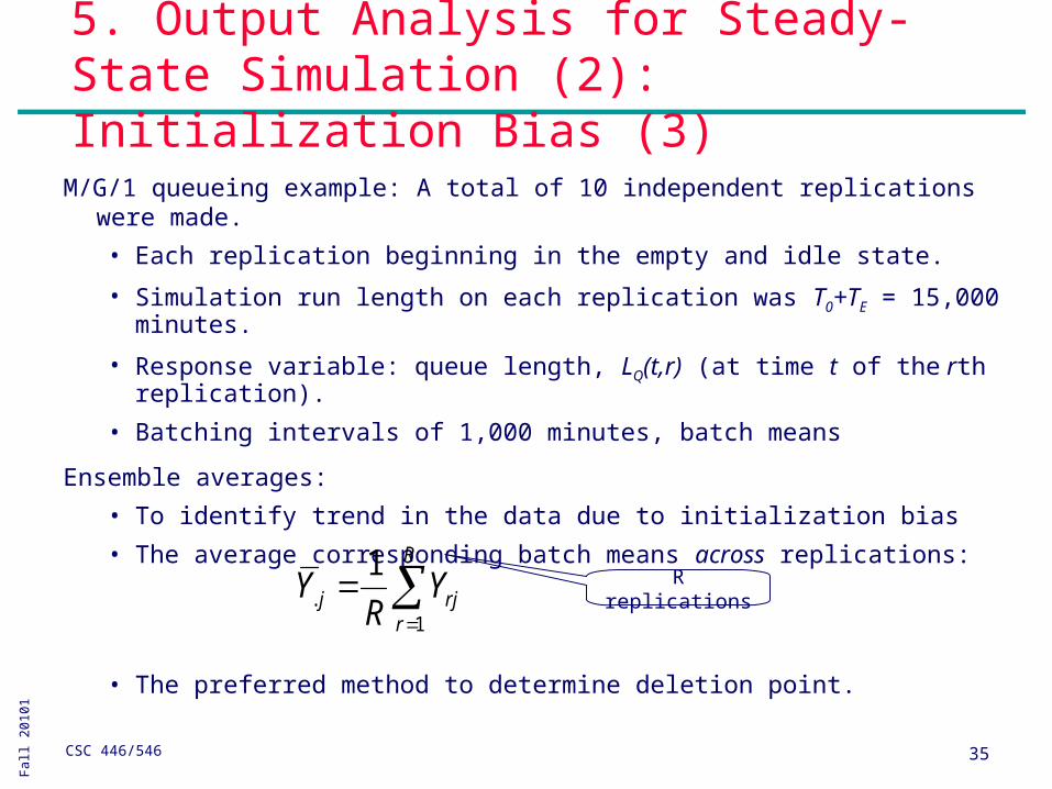
5. Output Analysis for Steady-State Simulation (2): Initialization Bias (3)
M/G/1 queueing example: A total of 10 independent replications were made.
• Each replication beginning in the empty and idle state.
• Simulation run length on each replication was T0+TE = 15,000 minutes.
• Response variable: queue length, LQ(t,r) (at time t of the rth replication).
• Batching intervals of 1,000 minutes, batch means
Ensemble averages:
• To identify trend in the data due to initialization bias
• The average corresponding batch means across replications:
• The preferred method to determine deletion point.
R
rrjj Y
RY
1.
1R replications
Fall
20
10
1
CSC 446/546 36
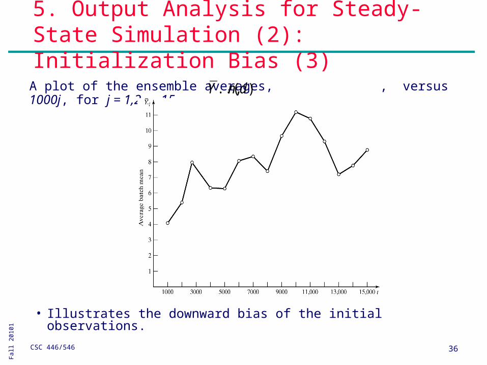
5. Output Analysis for Steady-State Simulation (2): Initialization Bias (3)
A plot of the ensemble averages, , versus 1000j, for j = 1,2, …,15.
• Illustrates the downward bias of the initial observations.
),..( dnY
Fall
20
10
1
CSC 446/546 37
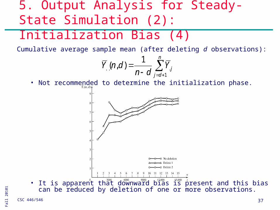
5. Output Analysis for Steady-State Simulation (2): Initialization Bias (4)
Cumulative average sample mean (after deleting d observations):
• Not recommended to determine the initialization phase.
• It is apparent that downward bias is present and this bias can be
reduced by deletion of one or more observations.
n
djjYdn
dnY1
...
1),(
Fall
20
10
1
CSC 446/546 38
5. Output Analysis for Steady-State Simulation (2): Initialization Bias (5)
No widely accepted, objective and proven technique to guide how much data to delete to reduce initialization bias to a negligible level.
Plots can, at times, be misleading but they are still recommended.
• Ensemble averages reveal a smoother and more precise trend as the # of replications, R, increases.
• Ensemble averages can be smoothed further by plotting a moving average.
• Cumulative average becomes less variable as more data are averaged.
• The more correlation present, the longer it takes for to approach steady state.
• Different performance measures could approach steady state at different rates.
jY.
Fall
20
10
1
CSC 446/546 39
5. Output Analysis for Steady-State Simulation (3): Error Estimation (1)
If {Y1, …, Yn} are not statistically independent, then S2/n is a biased estimator of the true variance.
• Almost always the case when {Y1, …, Yn} is a sequence of output observations from within a single replication (autocorrelated sequence, time-series).
Suppose the point estimator is the sample mean
• Variance of is almost impossible to estimate.
• For system with steady state, produce an output process that is approximately covariance stationary (after passing the transient phase).
– The covariance between two random variables in the time series depends only on the lag (the # of observations between them).
Y
n
i i nYY1
/
Fall
20
10
1
CSC 446/546 40
5. Output Analysis for Steady-State Simulation (3): Error Estimation (2)
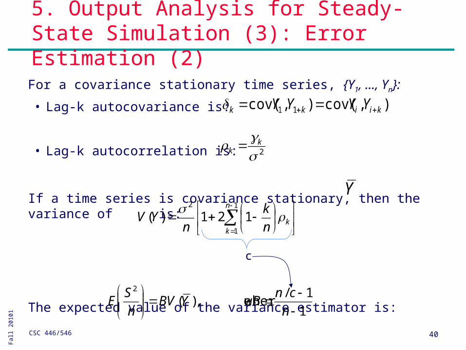
For a covariance stationary time series, {Y1, …, Yn}:
• Lag-k autocovariance is:
• Lag-k autocorrelation is:
If a time series is covariance stationary, then the variance of is:
The expected value of the variance estimator is:
Y
),cov(),cov( 11 kiikk YYYY
2 k
k
1
1
2
121)(n
kkn
k
nYV
1
1/ e wher,)(
2
n
cnBYBV
n
SE
c

Fall
20
10
1
CSC 446/546 41
5. Output Analysis for Steady-State Simulation (3): Error Estimation (3)
Stationary time series Yi exhibiting positive autocorrelation.
Stationary time series Yi
exhibiting negative autocorrelation.
Nonstationary time series with an upward trend

Fall
20
10
1
CSC 446/546 42
5. Output Analysis for Steady-State Simulation (3): Error Estimation (4)
The expected value of the variance estimator is:
• If Yi are independent, then S2/n is an unbiased estimator of
• If the autocorrelation k are primarily positive, then S2/n is biased low as an estimator of .
• If the autocorrelation k are primarily negative, then S2/n is biased high as an estimator of .
)(YV
of variance theis )( and 1
1/ e wher,)(
2
YYVn
cnBYBV
n
SE
)(YV
)(YV
Fall
20
10
1
CSC 446/546 43
5. Output Analysis for Steady-State Simulation (4): Replication Method (1)
Use to estimate point-estimator variability and to construct a confidence interval.
Approach: make R replications, initializing and deleting from each one the same way.
Important to do a thorough job of investigating the initial-condition bias:• Bias is not affected by the number of replications, instead, it
is affected only by deleting more data (i.e., increasing T0) or extending the length of each run (i.e. increasing TE).
Basic raw output data {Yrj, r = 1, ..., R; j = 1, …, n} is derived by:• Individual observation from within replication r.• Batch mean from within replication r of some number of
discrete-time observations.• Batch mean of a continuous-time process over time interval
j.

Fall
20
10
1
CSC 446/546 44
5. Output Analysis for Steady-State Simulation (4): Replication Method (2)
Each replication is regarded as a single sample for estimating For replication r:
The overall point estimator:
If d and n are chosen sufficiently large:
n,d ~ is an approximately unbiased estimator of .
To estimate standard error of , the sample variance and standard error:
n
djrjr Y
dndnY
1.
1),(
dn
R
rr dnYdnY
RdnY ,..
1... )],(E[ and ),(
1),(
),(.. dnY
R
SYesYRY
RYY
RS
R
rr
R
rr
).(. and 1
1)(
1
1..
1
2..
2.
1
2...
2
..Y
Fall
20
10
1
CSC 446/546 45
5. Output Analysis for Steady-State Simulation (4): Replication Method (3)
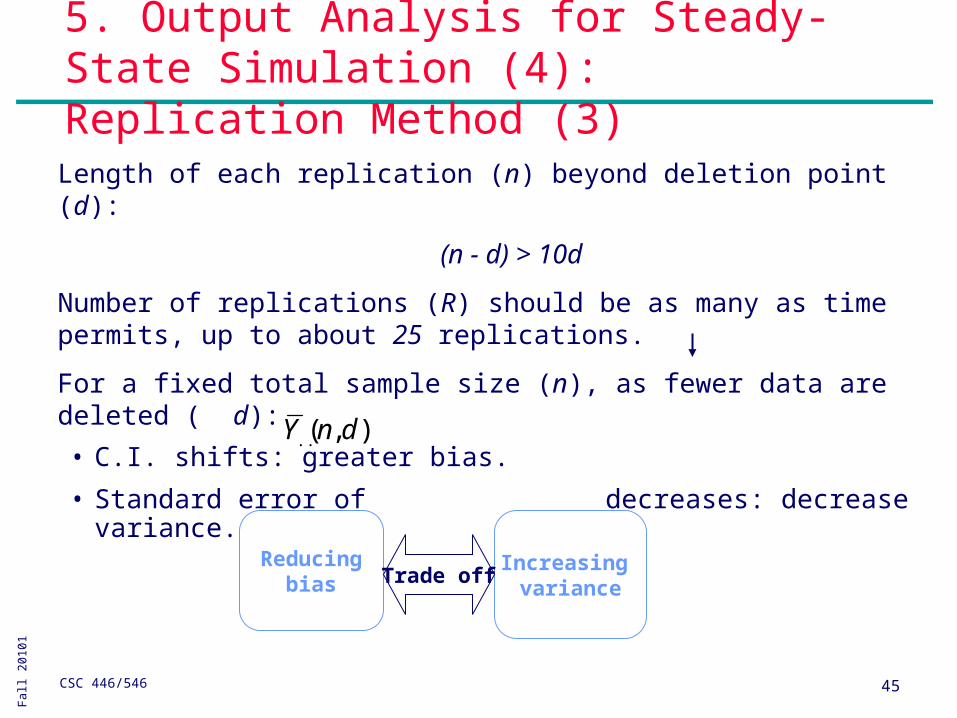
Length of each replication (n) beyond deletion point (d):
(n - d) > 10d
Number of replications (R) should be as many as time permits, up to about 25 replications.
For a fixed total sample size (n), as fewer data are deleted ( d):
• C.I. shifts: greater bias.
• Standard error of decreases: decrease variance.),(.. dnY
Reducingbias
Increasing variance
Trade off
Fall
20
10
1
CSC 446/546 46
5. Output Analysis for Steady-State Simulation (4): Replication Method (4)
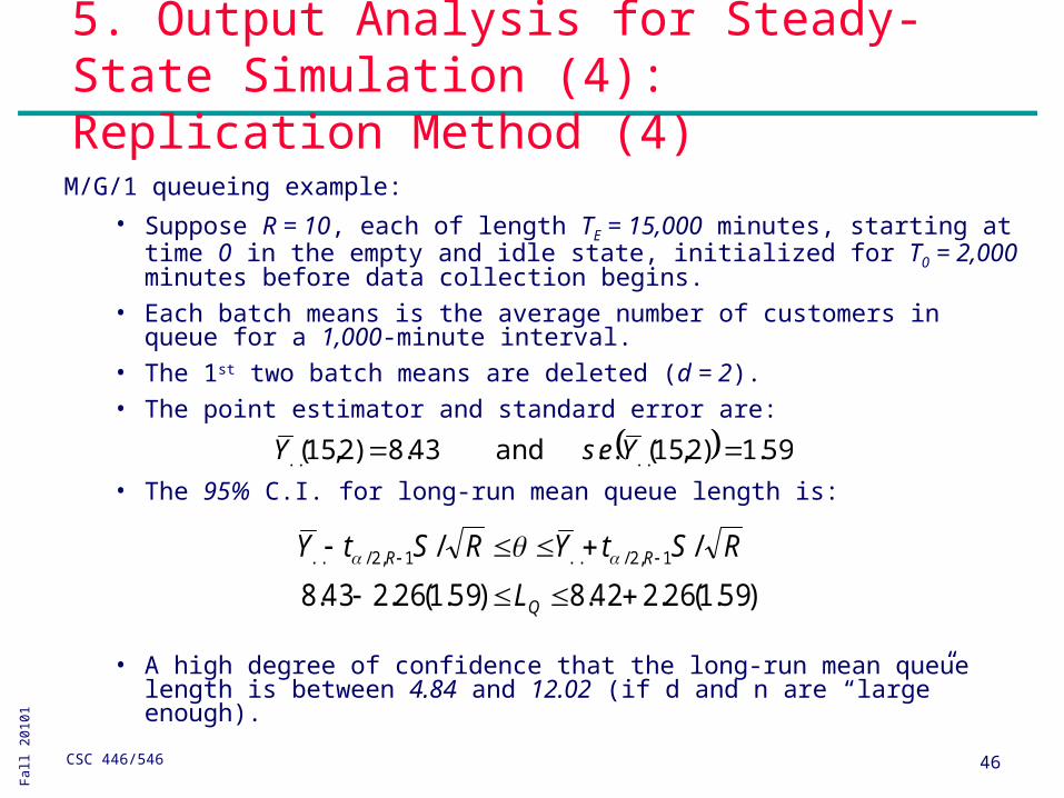
M/G/1 queueing example:
• Suppose R = 10, each of length TE = 15,000 minutes, starting at time 0 in the empty and idle state, initialized for T0 = 2,000 minutes before data collection begins.
• Each batch means is the average number of customers in queue for a 1,000-minute interval.
• The 1st two batch means are deleted (d = 2).• The point estimator and standard error are:
• The 95% C.I. for long-run mean queue length is:
• A high degree of confidence that the long-run mean queue length is between 4.84 and 12.02 (if d and n are “large” enough).
59.1)2,15(.. and 43.8)2,15( .... YesY
)59.1(26.242.8)59.1(26.243.8
// 1,2/..1,2/..
Q
RR
L
RStYRStY
Fall
20
10
1
CSC 446/546 47
5. Output Analysis for Steady-State Simulation (5): Sample Size (1)
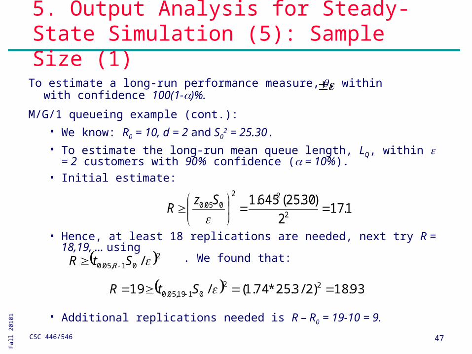
To estimate a long-run performance measure, , within with confidence 100(1-)%.
M/G/1 queueing example (cont.):
• We know: R0 = 10, d = 2 and S02 = 25.30.
• To estimate the long-run mean queue length, LQ, within = 2 customers with 90% confidence ( = 10%).
• Initial estimate:
• Hence, at least 18 replications are needed, next try R = 18,19, … using
. We found that:
• Additional replications needed is R – R0 = 19-10 = 9.
1.172
)30.25(645.12
22
005.0
Sz
R
93.18)2/3.25*74.1(/19 220119,05.0 StR
201,05.0 /StR R
Fall
20
10
1
CSC 446/546 48
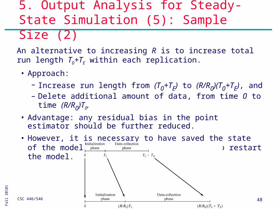
5. Output Analysis for Steady-State Simulation (5): Sample Size (2)
An alternative to increasing R is to increase total run length T0+TE within each replication.
• Approach:– Increase run length from (T0+TE) to (R/R0)(T0+TE), and– Delete additional amount of data, from time 0 to time
(R/R0)T0.
• Advantage: any residual bias in the point estimator should be further reduced.
• However, it is necessary to have saved the state of the model at time T0+TE and to be able to restart the model.
Fall
20
10
1
CSC 446/546 49
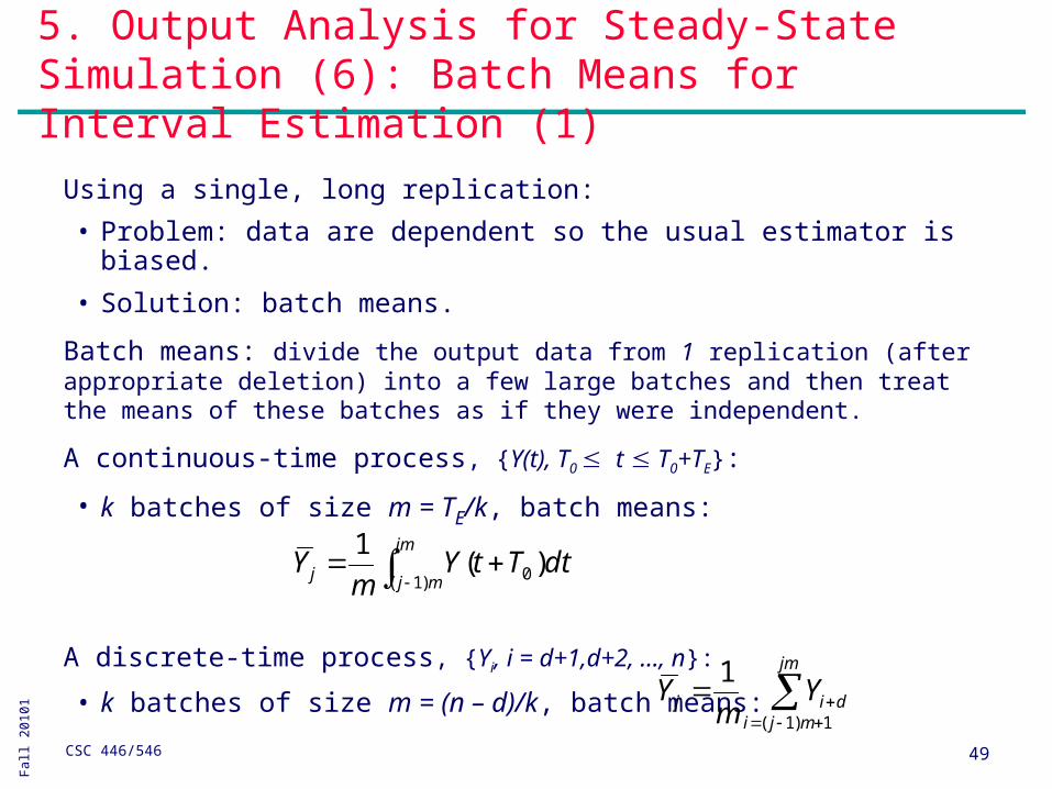
5. Output Analysis for Steady-State Simulation (6): Batch Means for Interval Estimation (1)
Using a single, long replication:
• Problem: data are dependent so the usual estimator is biased.
• Solution: batch means.
Batch means: divide the output data from 1 replication (after appropriate deletion) into a few large batches and then treat the means of these batches as if they were independent.
A continuous-time process, {Y(t), T0 t T0+TE}:
• k batches of size m = TE/k, batch means:
A discrete-time process, {Yi, i = d+1,d+2, …, n}:
• k batches of size m = (n – d)/k, batch means:
jm
mjidij Y
mY
1)1(
1
jm
mjj dtTtYm
Y)1( 0 )(
1
Fall
20
10
1
CSC 446/546 50
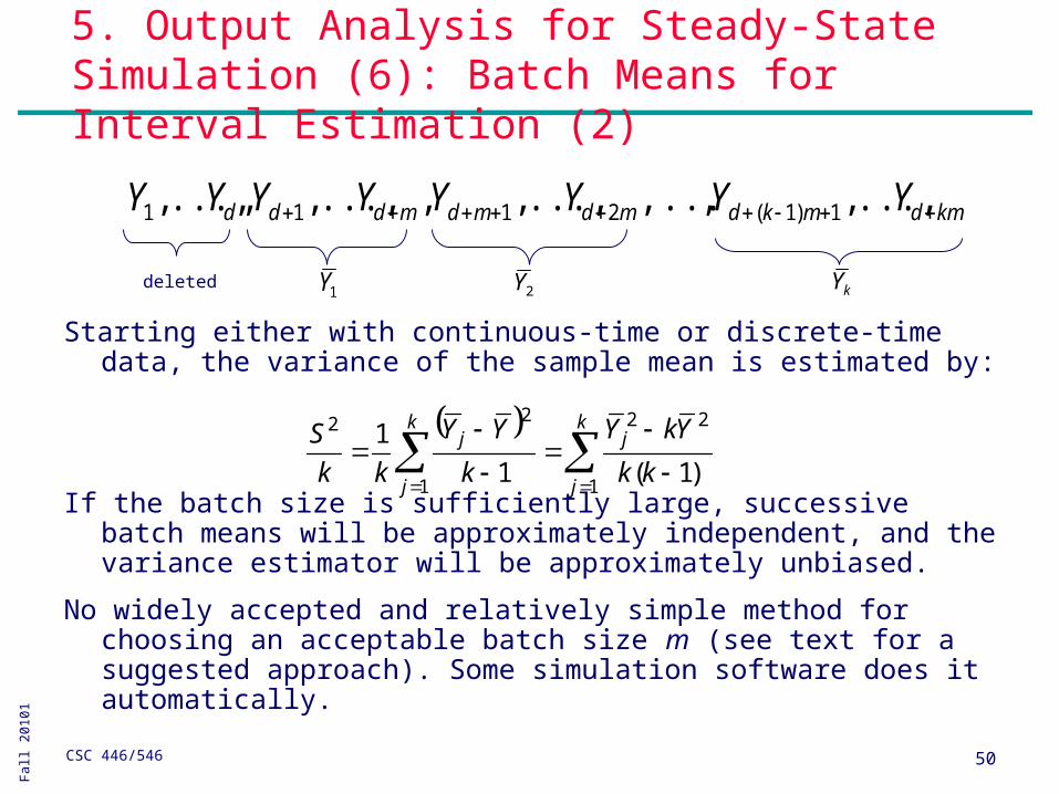
5. Output Analysis for Steady-State Simulation (6): Batch Means for Interval Estimation (2)
Starting either with continuous-time or discrete-time data, the variance of the sample mean is estimated by:
If the batch size is sufficiently large, successive batch means will be approximately independent, and the variance estimator will be approximately unbiased.
No widely accepted and relatively simple method for choosing an acceptable batch size m (see text for a suggested approach). Some simulation software does it automatically.
kmdmkdmdmdmddd YYYYYYYY ..., ,, ... ,..., ,,..., ,,..., , 1)1(2111
k
j
jk
j
j
kk
YkY
k
YY
kk
S
1
22
1
22
)1(1
1
deleted1Y 2Y kY