Extreme Flooding, Policy Development, and Feedback Modelling

Evan Davies and Slobodan SimonovicCivil and Environmental Engineering

The University of Western Ontario

London ON Canada

Flood 2008 Conference

Presentation Outline

Introduction Model Description Experimentation Conclusions

Introduction: Goals

1. Develop integrated model and apply to extreme flooding

2. Simulate long-term impacts of extreme flooding on socio-economic and natural systems

3. Stress importance of feedbacks

Understanding better policy

Society

EconomyEnvironment

Introduction

Natural Change Socio-economic Change

Extreme Flood

Rationale

Floods are basically naturalPrecipitationRunoff

Hazard is of human-originSettlement patternsLand-use patternsFlood defences

Introduction

Feedbacks and Extreme Flooding

In flooding, natural and anthropogenic systems interactRealization underlies IFM

Integrated Assessment approachFeedback is crucial Simulation modelling!Simulation modelling!

Introduction

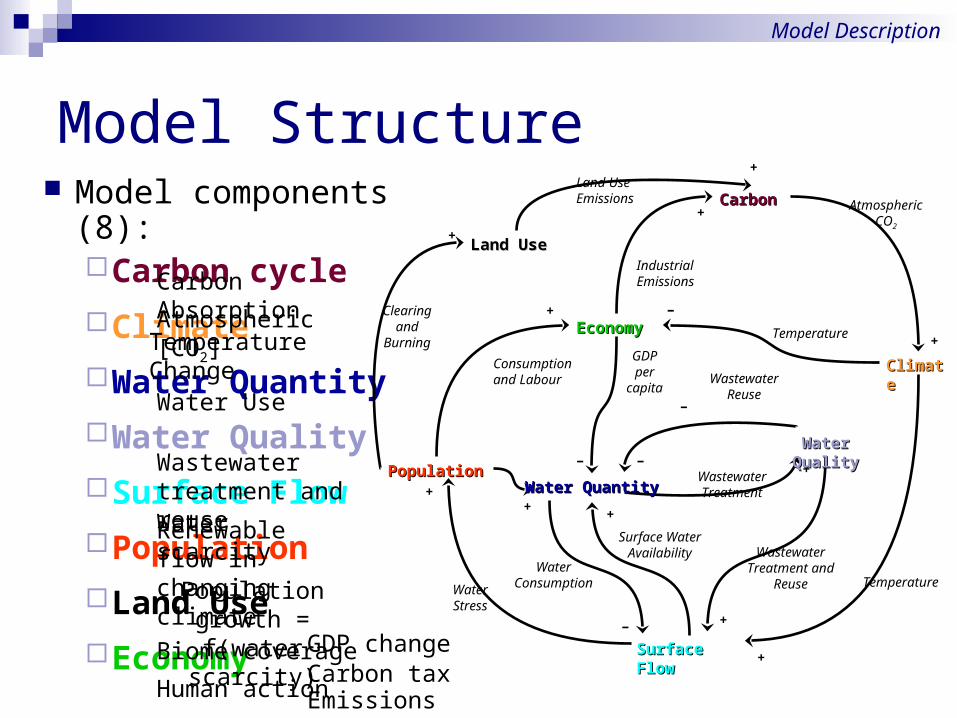
Model Structure Model components (8):

Carbon cycle

Climate

Water Quantity

Water Quality

Surface Flow

Population

Land Use

Economy

Clearing and

Burning

Land Use Emissions

+

CarbonCarbon

ClimateClimate

+

+

+

Land UseLand Use

+

+

Temperature

Atmospheric CO2

Water Stress

Industrial Emissions

−

Surface Water Availability

Water Consumption

PopulationPopulation

EconomyEconomy

Surface FlowSurface Flow

Temperature

Consumption and Labour

+

+ −

GDP per

capita

+

Water QualityWater Quality

Water QuantityWater QuantityWastewaterTreatment

WastewaterReuse

WastewaterTreatment and

Reuse

−

−

+

+

−

Carbon Absorption

Atmospheric [CO2]Temperature Change

Water Use

Wastewater treatment and reuseWater scarcityRenewable flow in changing climatePopulation growth = f(water scarcity)Biome coverage

Human action

GDP changeCarbon taxEmissions

Model Description

Model Characteristics

Number of Model Elements: 740 named variables

‘Variables’: ~1600 (incl. arrays) Constants: ~470 (incl. arrays)

230 Stocks (many in arrays) 2300 total

600 equations (99 are critical) Thousands of feedbacks

Population: 4468 loops Water stress: 2756 loops Economic output: 203 loops Industrial emissions: 47 loops

Model Description

Work in Context

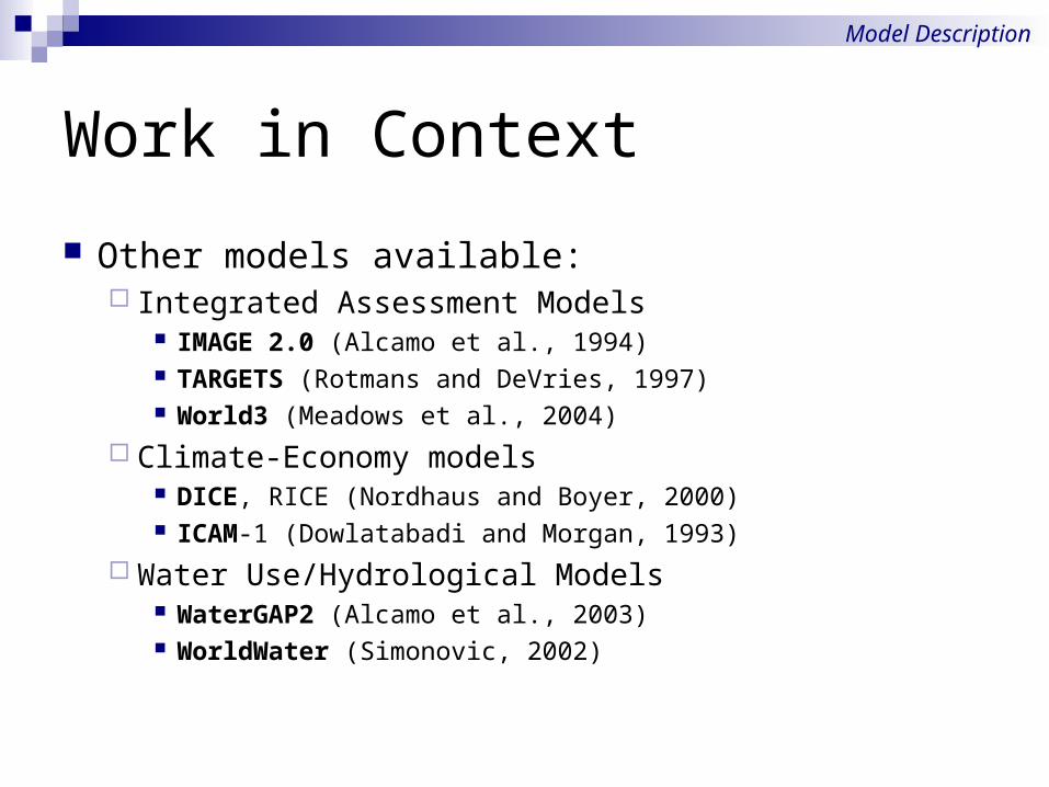
Other models available: Integrated Assessment Models

IMAGE 2.0 (Alcamo et al., 1994) TARGETS (Rotmans and DeVries, 1997) World3 (Meadows et al., 2004)

Climate-Economy models DICE, RICE (Nordhaus and Boyer, 2000) ICAM-1 (Dowlatabadi and Morgan, 1993)

Water Use/Hydrological Models WaterGAP2 (Alcamo et al., 2003) WorldWater (Simonovic, 2002)

Model Description

Simulating Flooding

Floods affect:Water quality InfrastructureAgriculture and crops(Human health)

But to different degrees…

Experimental Approach

Experiments

Run three experiments Small flood Medium flood Large flood

One year duration of direct effects Global ResolutionGlobal Resolution Annual CycleAnnual Cycle

Compare with Base Case

Experimental Approach

Capital

Irrigated land

Wastewater Treatment

Water Reuse

Agricultural Pollution

Impose change on:

Results: Direct Effects

After one year, changes in Available surface waterCapital stock Irrigated areaWastewater treatmentWastewater reuseWater withdrawals

Results

Irrigated Area

300 M

250 M

200 M

2005 2007 2009 2011 2013 2015Time (Year)

Irrigated Area : Base haIrrigated Area : Small haIrrigated Area : Medium haIrrigated Area : Large ha

Capital K(t)

100

80

60

2005 2007 2009 2011 2013 2015Time (Year)

"Capital K(t)" : Base trillion $"Capital K(t)" : Small trillion $"Capital K(t)" : Medium trillion $"Capital K(t)" : Large trillion $

Available Surface Water

20,000

15,000

10,000

2005 2007 2009 2011 2013 2015Time (Year)

Available Surface Water : Base km*km*km/YearAvailable Surface Water : Small km*km*km/YearAvailable Surface Water : Medium km*km*km/YearAvailable Surface Water : Large km*km*km/Year

Untreated Returnable Waters

1,102

951.45

800

2005 2007 2009 2011 2013 2015Time (Year)

Untreated Returnable Waters : Base km*km*km/YearUntreated Returnable Waters : Small km*km*km/YearUntreated Returnable Waters : Medium km*km*km/YearUntreated Returnable Waters : Large km*km*km/Year

INDIRECT Effects

The focus of the exercise…

The flooding causesNo behavioural changeLong-lasting damage

Results

Total Wastewater Reuse

1,000

500

0

2005 2020 2035 2050 2065 2080 2095Time (Year)

Total Wastewater Reuse : Base km*km*km/YearTotal Wastewater Reuse : Small km*km*km/YearTotal Wastewater Reuse : Medium km*km*km/YearTotal Wastewater Reuse : Large km*km*km/Year

Capital K(t)

200

125.24

50.48

2004 2016 2027 2039 2050Time (Year)

"Capital K(t)" : Base trillion $"Capital K(t)" : Small trillion $"Capital K(t)" : Medium trillion $"Capital K(t)" : Large trillion $

Surface Water Withdrawals

4,500

4,250

4,000

2005 2015 2025 2035 2045 2055 2065 2075 2085 2095Time (Year)

Surface Water Withdrawals : Base km*km*km/YearSurface Water Withdrawals : Small km*km*km/YearSurface Water Withdrawals : Medium km*km*km/YearSurface Water Withdrawals : Large km*km*km/Year

Indirect Effects

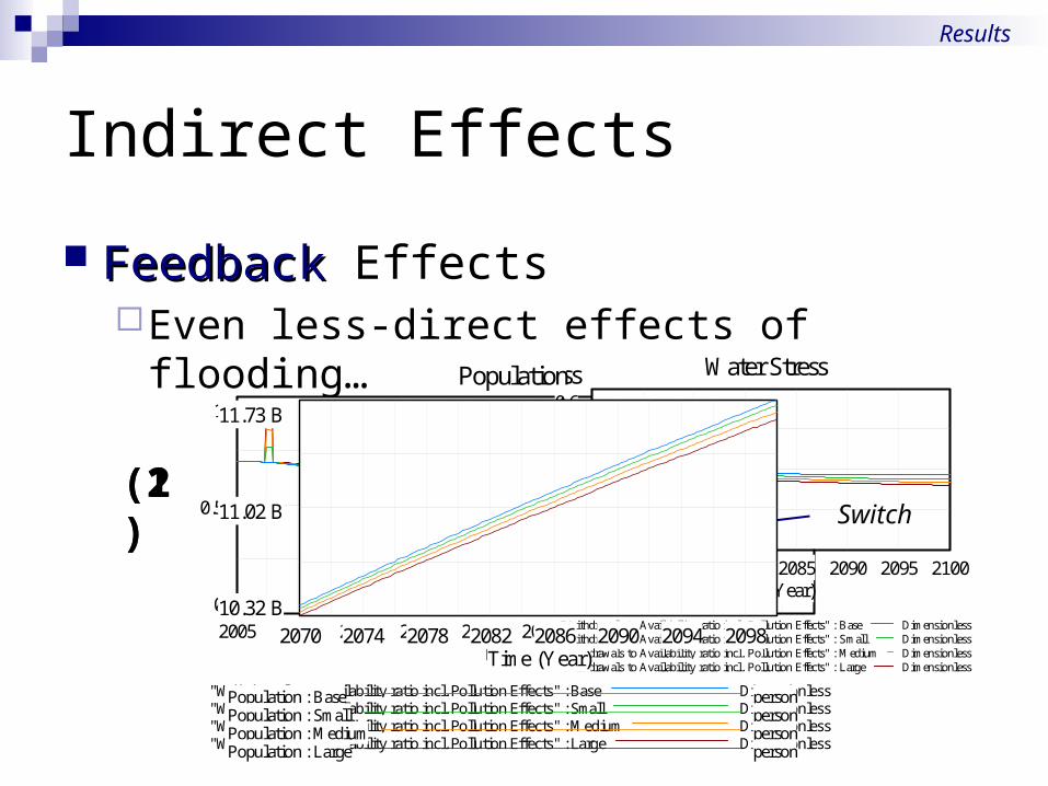
FeedbackFeedback EffectsEven less-direct effects of flooding…

Results

Water Stress

1

0.5

0

2005 2015 2025 2035 2045 2055 2065 2075 2085 2095Time (Year)

"Withdrawals to Availability ratio incl. Pollution Effects" : Base Dimensionless"Withdrawals to Availability ratio incl. Pollution Effects" : Small Dimensionless"Withdrawals to Availability ratio incl. Pollution Effects" : Medium Dimensionless"Withdrawals to Availability ratio incl. Pollution Effects" : Large Dimensionless

Water Stress

0.6

0.4

0.2

2065 2070 2075 2080 2085 2090 2095 2100Time (Year)

"Withdrawals to Availability ratio incl. Pollution Effects" : Base Dimensionless"Withdrawals to Availability ratio incl. Pollution Effects" : Small Dimensionless"Withdrawals to Availability ratio incl. Pollution Effects" : Medium Dimensionless"Withdrawals to Availability ratio incl. Pollution Effects" : Large Dimensionless

Switch

Population

11.73 B

11.02 B

10.32 B2070 2074 2078 2082 2086 2090 2094 2098

Time (Year)

Population : Base personPopulation : Small personPopulation : Medium personPopulation : Large person

(1)(2)

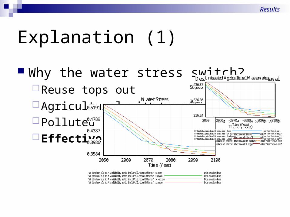
Explanation (1)

Why the water stress switch?Reuse tops outAgricultural withdrawalsPolluted surface waterEffective Withdrawal

Total Wastewater Reuse

976.95

692.60

408.252050 2060 2070 2080 2090 2100

Time (Year)

Total Wastewater Reuse : Base km*km*km/YearTotal Wastewater Reuse : Small km*km*km/YearTotal Wastewater Reuse : Medium km*km*km/YearTotal Wastewater Reuse : Large km*km*km/Year

Desired Agricultural Water Withdrawal

2,491

2,362

2,2342050 2060 2070 2080 2090 2100

Time (Year)

Desired Agricultural Water Withdrawal : Base km*km*km/YearDesired Agricultural Water Withdrawal : Small km*km*km/YearDesired Agricultural Water Withdrawal : Medium km*km*km/YearDesired Agricultural Water Withdrawal : Large km*km*km/Year

Polluted Returnable Water

508.30

365.46

222.622050 2060 2070 2080 2090 2100

Time (Year)

Untreated Returnable Waters : Base km*km*km/YearUntreated Returnable Waters : Small km*km*km/YearUntreated Returnable Waters : Medium km*km*km/YearUntreated Returnable Waters : Large km*km*km/Year

Effective Water Withdrawal

8,003

6,807

5,6112050 2060 2070 2080 2090 2100

Time (Year)

Effective Desired Surface Water Withdrawal : Base km*km*km/YearEffective Desired Surface Water Withdrawal : Small km*km*km/YearEffective Desired Surface Water Withdrawal : Medium km*km*km/YearEffective Desired Surface Water Withdrawal : Large km*km*km/Year

Results

Water Stress

0.5191

0.4789

0.4387

0.3986

0.35842050 2060 2070 2080 2090 2100

Time (Year)

"Withdrawals to Availability ratio incl. Pollution Effects" : Base Dimensionless"Withdrawals to Availability ratio incl. Pollution Effects" : Small Dimensionless"Withdrawals to Availability ratio incl. Pollution Effects" : Medium Dimensionless"Withdrawals to Availability ratio incl. Pollution Effects" : Large Dimensionless

Untreated Agricultural Wastewater

436.37

326.30

216.24

2050 2060 2070 2080 2090 2100Time (Year)

Untreated Agricultural Wastewater : Base km*km*km/YearUntreated Agricultural Wastewater : Small km*km*km/YearUntreated Agricultural Wastewater : Medium km*km*km/YearUntreated Agricultural Wastewater : Large km*km*km/Year

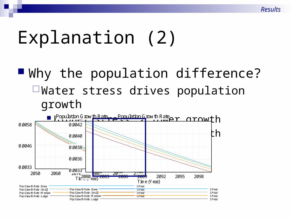
Explanation (2)

Why the population difference?Water stress drives population growth

Higher stress lower growth Lower stress higher growth

Results

Population Growth Rate

0.0058

0.0046

0.00332050 2060 2070 2080 2090 2100

Time (Year)

Pop Growth Rate : Base 1/YearPop Growth Rate : Small 1/YearPop Growth Rate : Medium 1/YearPop Growth Rate : Large 1/Year

Population Growth Rate

0.0042

0.0040

0.0038

0.0036

0.00332080 2083 2086 2089 2092 2095 2098

Time (Year)

Pop Growth Rate : Base 1/YearPop Growth Rate : Small 1/YearPop Growth Rate : Medium 1/YearPop Growth Rate : Large 1/Year

Conclusions

Developed feedbackfeedback-based-based model Physical and socio-economic sectors Closed-loop structure

Flood Experiments Impose direct effects, simulate long-term Long-term damage to

Infrastructure, Water quality Led to

Higher water stress Lower population

Illustrate IA modelling framework

Conclusions

Cost of the approach:Sacrifice resolution for completeness

Benefits of the approach:Connect Socio-economic and Physical Systems Identify and understand causesAnalyze system behaviour

Publications

Model structure, behaviour & applications

Available from

http://publish.uwo.ca/~edavies7