Copyright © 2011 by Pearson Education Inc. publishing as Prentice Hall. All rights reserved.From Skills for Success with Microsoft® Excel 2010 Comprehensive

Manage Multiple Worksheets | Microsoft Excel Chapter 3 More Skills: SKILL 12 | Page 1 of 5

� A line chart displays trends over time. Time is displayed along the bottom axis, and the datapoint values are connected with a line.

� To allow you to compare more than one set of values, each group of values is connected by a different line. The curves and directions of the lines emphasize trends over time.

To complete this workbook, you will need the following file:� e03_Growth

You will save your workbook as:� Lastname_Firstname_e03_Growth

1. Start Excel. From your student data files, open e03_Growth. Save the workbook in yourExcel Chapter 3 folder as Lastname_Firstname_e03_Growth

2. Add the file name in the worksheet’s left footer, and then return to Normal view.

3. Select the range A4:F7. On the Insert tab, in the Charts group, click the Line button.From the Chart gallery, under 2-D Line, click the first chart in the second row—Line with Markers.

ExcelCHAPTER 3

More Skills 12 Create Line Charts

Copyright © 2011 by Pearson Education Inc. publishing as Prentice Hall. All rights reserved.From Skills for Success with Microsoft® Excel 2010 Comprehensive

Manage Multiple Worksheets | Microsoft Excel Chapter 3 More Skills: SKILL 12 | Page 2 of 5

4. On the Design tab, in the Location group, click the Move Chart button. In the displayedMove Chart dialog box, select the New Sheet option button, replace the text with GrowthChart and then click OK. On the Insert tab, in the Text group, click the Header & Footerbutton. In the Page Setup dialog box, click the Custom Footer button. Click the Insert FileName button , and then click OK two times. Compare your screen with Figure 1.

Excel considers the dates in row 4 to be numbers and will plot row 4, the EstimatedGrowth Rate. This chart line displays along the horizontal axis on the bottom of thechart.

Chart displayson chart sheet

Row 4 plotted

Figure 1

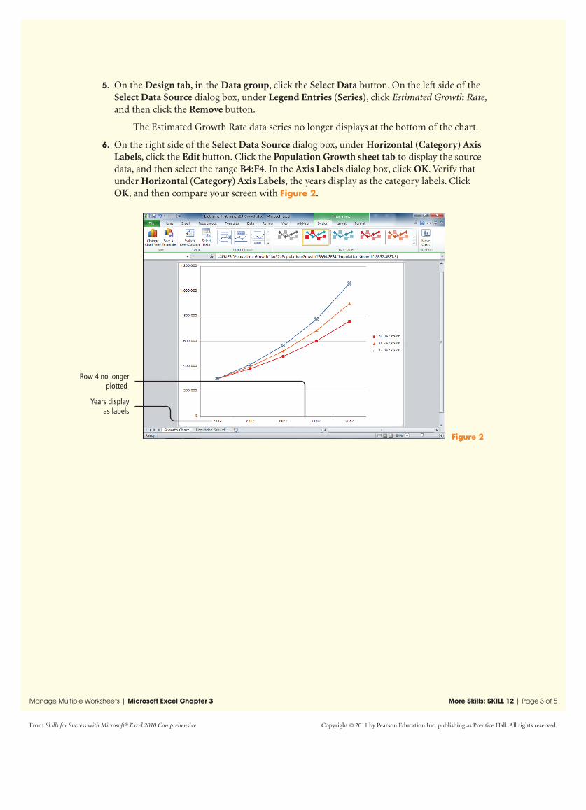
5. On the Design tab, in the Data group, click the Select Data button. On the left side of theSelect Data Source dialog box, under Legend Entries (Series), click Estimated Growth Rate,and then click the Remove button.

The Estimated Growth Rate data series no longer displays at the bottom of the chart.

6. On the right side of the Select Data Source dialog box, under Horizontal (Category) AxisLabels, click the Edit button. Click the Population Growth sheet tab to display the sourcedata, and then select the range B4:F4. In the Axis Labels dialog box, click OK. Verify thatunder Horizontal (Category) Axis Labels, the years display as the category labels. ClickOK, and then compare your screen with Figure 2.

Copyright © 2011 by Pearson Education Inc. publishing as Prentice Hall. All rights reserved.From Skills for Success with Microsoft® Excel 2010 Comprehensive

Manage Multiple Worksheets | Microsoft Excel Chapter 3 More Skills: SKILL 12 | Page 3 of 5

Figure 2

Years displayas labels

Row 4 no longerplotted

Copyright © 2011 by Pearson Education Inc. publishing as Prentice Hall. All rights reserved.From Skills for Success with Microsoft® Excel 2010 Comprehensive

Manage Multiple Worksheets | Microsoft Excel Chapter 3 More Skills: SKILL 12 | Page 4 of 5

7. On the Design tab, in the Chart Layouts group, click the More button , and then clickLayout 10. In the Chart Styles group, click the More button , and then click Style 35.

8. At the top of the chart, click the Chart Title, type Aspen Falls Growth Estimates and thenpress J.

9. At the left side of the chart, click the vertical Axis Title, type Population and then press J.Right-click the vertical Axis Title, and then on the Mini toolbar, change the Font Size to 12.

10. At the bottom of the chart, click the horizontal Axis Title, type Years and then press J.Right-click the horizontal Axis Title, and then on the Mini toolbar, change the Font Sizeto 12.

11. On the Layout tab, in the Current Selection group, click the Chart Element arrow, andthen click Chart Area. In the Current Selection group, click the Format Selection button.In the Format Chart Area dialog box, under Fill, select the Gradient fill option button.Under Gradient stops, click the Stop 1 of 3 button, and then compare your screen withFigure 3.

Figure 3

Stop 1 of 3 button

Color button

Gradient filloption button

Chart Elementarrow

12. Click the Color button, and then click the fifth color in the first row—Turquoise, Accent 1.

13. Click the Stop 2 of 3 button, click the Color button, and then click the fifth color in thethird row—Turquoise, Accent 1, Lighter 60%. Close the dialog box, and then compareyour screen with Figure 4.

Copyright © 2011 by Pearson Education Inc. publishing as Prentice Hall. All rights reserved.From Skills for Success with Microsoft® Excel 2010 Comprehensive

Manage Multiple Worksheets | Microsoft Excel Chapter 3 More Skills: SKILL 12 | Page 5 of 5

14. Save the workbook. Print or submit the file as directed by your instructor. Exit Excel.

� You have completed More Skills 12

Figure 4

Gradient fill color