evaluation of a stochastic weather generator in different climates

www.ccsenet.org/cis Computer and Information Science Vol. 3, No. 3; August 2010

Published by Canadian Center of Science and Education 217

Evaluation of a Stochastic Weather Generator in Different Climates Behnam Ababaei (Corresponding author)

PhD Student, Irrigation and Drainage Engineering Member of Young Researchers Club of Islamic Azad University

Science and Research Branch of Tehran, Iran Tel: 98-21-4413-1066 E-mail: [email protected]

Teymour Sohrabi

Professor, Department of Irrigation and Reclamation Faculty of Agricultural Engineering and Technology, University of Tehran, Karaj, Iran

E-mail: [email protected]

Farhad Mirzaei Assistant Professor, Department of Irrigation and Reclamation

Faculty of Agricultural Engineering and Technology University of Tehran, Karaj, Iran E-mail: [email protected]

Bakhtiar Karimi

PhD Student, Irrigation and Drainage Engineering Member of Young Researchers Club of Islamic Azad University

Branch of Kermanshah, Iran E-mail: [email protected]

Abstract Stochastic weather generators are used in different studies which often require long series of daily weather data for risk assessment. They can produce synthetic daily time series of any length. Any generator should be tested to ensure that the synthetic data is proper for the purposes for which it is to be used. The main objective of this paper is to test a stochastic weather generator, LARS-WG, at 65 sites in Iran chosen to represent different climates. Statistical tests were carried out to compare characteristics of the observed and synthetic weather data such as, the lengths of wet and dry series, the distribution of precipitation and the lengths of frost periods. The LARS-WG generator uses complex semi-empirical distributions for weather variables and tended to match the observed data well, especially in terms of the daily distributions and the mean monthly values, although there are certain characteristics of the data that the generator could not reproduce accurately, for example the monthly standard deviations. LARS-WG model showed different performance in different climates and stations. Therefore, evaluation is strongly recommended if it is going to be used in different climates and stations. Keywords: LARS-WG, Weather generator, Evaluation, Different climates, Iran 1. Introduction Weather generators are models that replicate the statistical attributes of local climate variables but they don’t reproduce observed sequences of events (Wilks et al., 1999; Wilby et al., 2004). There are several reasons for the development of stochastic weather generators and for the use of synthetic weather data instead of observed. The first one is to generate weather data time series long enough to be used in a risk assessment in hydrological and agricultural applications. Observed daily weather is one of the major inputs into mathematical and agrohydrological models, but the length of the time series is often insufficient to evaluate the probability of extreme events. Moreover, observed time series represent only one ‘realization’ of the climate, whereas a weather generator can simulate many ‘realizations’ and then, a wider range of feasible situations. The second reason is to provide the means for extending the simulation of weather to locations where observed weather data is not available by interpolating the parameters of a weather generator between sites using an interpolation


ISSN 1913-8989 E-ISSN 1913-8997 218

technique such as kriging (Hutchinson, 1995). A third area of application is in climate change studies. The output obtained from Global Climate Models (GCMs) cannot be used directly at a site due to their large spatial scale (Wilby et al., 2004). Daily scenario data can then be obtained by running the weather generator using this revised set of parameters such as climatic means and climate variability predicted by the GCMs (Wilks, 1992; Semenov and Barrow, 1997). Weather generators are becoming a standard component of decision support systems in a wide range of studies. There is a danger that generators will be used ‘as supplied’, i.e. without sufficient validation performed for the sites at which they are applied (Semenov et al., 1998). Most weather generators have been tested intensively, but usually only for one country or one region. The main objective of this study is to evaluate the performance of a popular stochastic weather generator model LARS-WG in 65 stations of Iran belonging to diverse climates. 2. Materials and Methods 2.1 LARS-WG Model Description The first version of the LARS-WG weather generator was developed in Budapest in 1990 as part of Assessment of Agricultural Risk in Hungary, a project funded by the Hungarian Academy of Sciences (Racsko et al., 1991; Semenov and Barrow, 2002). The focus of this work was to overcome the limitations of the Markov chain model of precipitation occurrence (Bailey, 1964; Richardson, 1981). This method of precipitation occurrence modeling which generally considers two precipitation states, wet or dry, and only considers conditions on the previous day is not always able to correctly simulate the maximum dry spell length which is crucial for a realistic assessment of agricultural production in some regions of the world. This resulted in the new ‘series’ approach in which the simulation of dry and wet spell length is the first step in the weather generation process. A modified version of this weather generator, now called LARS-WG (Long Ashton Research Station Weather Generator - the location at which it was developed in its current form), was used in the construction of the climate change scenarios used in two major European Union-funded research projects examining the impacts of climate change on agricultural potential in Europe, i.e., CLAIRE (Harrison et al., 1995) and CLIVARA (Downing et al., 2000). LARS-WG is based on the series weather generator described in Racsko et al. (1991). Table 1 shows the different procedures used in LARS-WG. It utilizes semi-empirical distributions (SED) for the lengths of wet and dry day series, daily precipitation, minimum and maximum temperature and daily solar radiation. The semi-empirical distribution Emp= {a0, ai; hi, i=1,.…,23}, is a histogram with 23 intervals, [ai-1, ai), where ai-1 < ai, and hi denotes the number of events from the observed data in the i-th interval. Random values from the semi-empirical distributions are chosen by first selecting one of the intervals (using the proportion of events in each interval as the selection probability), and then selecting a value within that interval from the uniform distribution. Such a distribution is flexible and can approximate a wide variety of shapes by adjusting the intervals [ai-1, ai). The cost of this flexibility, however, is that the distribution requires many parameters (24 parameters for the edges and 23 parameters for the number of events in each interval) to be specified compared with, for example, 3 parameters for the mixed-exponential distribution used in an earlier version of the model to define the dry and wet day series (Racsko et al., 1991). To approximate the extreme values of a climatic variable accurately, some intervals are assigned close to 0 for extreme low values of the variable and close to 1 for extreme high values; the remaining intervals are distributed evenly on the probability scale. The simulation of precipitation occurrence is modeled as alternate wet and dry series, where a wet day is defined to be a day with precipitation > 0.0 mm. The length of each series is chosen randomly from the wet or dry semi-empirical distribution for the month in which the series starts. In determining the distributions, observed series are also allocated to the month in which they start. For a wet day, the precipitation value is generated from the semi-empirical precipitation distribution for the particular month independent of the length of the wet series or the amount of precipitation on previous days. In the previous version of LARS-WG, normalized residuals of maximum and minimum temperature (separate for dry and wet days) were approximated by the Normal distribution with the monthly means and standard deviation approximated by the Fourier series. It has been shown (Semenov and Stratonovitch, 2009; Qian et al., 2004; Semenov, 2008) that for locations where temperature residuals are not normally distributed, simulation of extreme high or low temperatures could be poor compared with the observed data. In the LARS-WG version 5.0, the maximum and minimum temperatures for dry and wet days are approximated by semi-empirical distributions calculated for each month, with auto- and cross-correlations calculated monthly (previously, only one, annual, auto- and cross- correlation coefficients was used). The introduction of these changes has significantly improved the simulation of extreme temperatures (Semenov and Stratonovitch, 2009). Semi-empirical distributions for climatic variables are calculated on a monthly basis by LARS-WG. Some of the variables follow an annual cycle. To reproduce a smooth seasonal



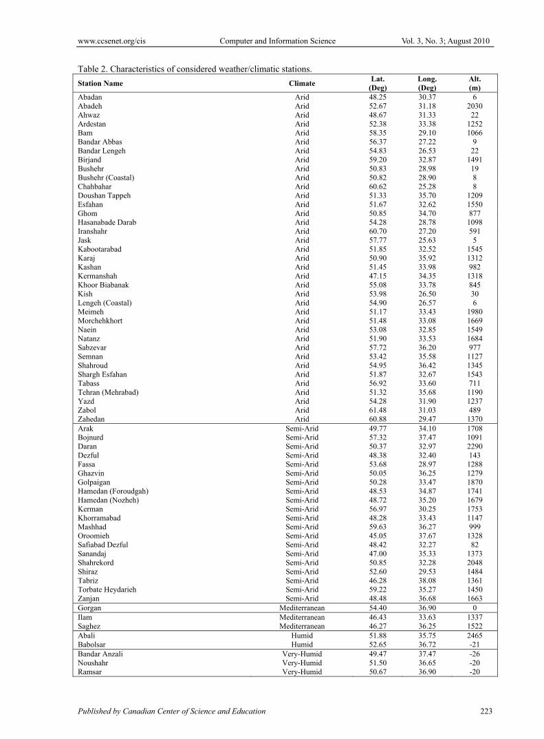
cycle of daily minimum or maximum temperature and daily radiation, the SED is computed for a given day by interpolating between two monthly SEDs. The resulting distribution for each month is a weighted sum of the distributions of the current and the previous or next month. LARS-WG accepts sunshine hours as an alternative to solar radiation data. If solar radiation data are unavailable, then sunshine hours may be automatically converted to solar radiation using the approach described in Rietveld (1978). For more details on LARS-WG 5.0 see Semenov and Stratonovitch (2009). 2.2 Sites Description Iran is located in the Middle East and is mostly consisted of arid and semi arid regions. But humid regions can be found in the northern parts of the country. The study was carried out for 65 weather/climatic stations across Iran (Table 2); each station had different record period and quality. LARSWG can operate with as little as 1 yr of data (Semenov et al., 1998). However, fairly long records are required to calculate robust and representative generator parameters for the site. The number of years of available data ranged from 3 at Lengeh (Coastal) to 51 at Abadan and Ahwaz. A few stations have missing data in some months or even in the entire year specifically for radiation time series. Ideally, weather variables should be measured directly at each site, rather than being estimated from the other variables. Unfortunately, measured solar radiation is not available at several sites in the earlier years of record. However, where sunshine hours were available, the missing solar radiation values were estimated from sunshine hours or cloud cover using the regression methods of Rietveld (1978) and Doorenbos and Pruit (Doorenbos and Pruit, 1984), respectively. In the absence of this information, the solar radiation values for those years were treated as missing and the solar radiation parameters calculated from the remaining data. LARS-WG automatically ignores missing values and converts sunshine hours to radiation (Semenov et al., 1998). The stations were classified using the method of De Martonne (Equation 1 and Table 3):

[1] 10+

=T

PI

Where P is mean annual precipitation (mm) and T is mean annual temperature (oC). According to this, 37 stations (out of 65) are located in Arid regions, 20 stations in Semi-Arid regions, 3 in Mediterranean and 5 stations are located in Humid and Very-Humid regions. 2.3 Statistical Tests In order to evaluate the performance of LARS-WG model, proper statistical tests were done to compare observed and synthetic time series. This included two different steps: 1) Observed data series were analyzed by the model and required statistics were calculated. 2) Using calculated statistics, LARS-WG was used to generate synthetic time series for a period of 500 years for all the stations. Such a long series of data was used so that the statistical properties of the synthetic data would be close to the true distribution of the data produced by the generators. A longer data series makes the statistical tests more powerful since they are then more likely to give a significant result when there is a difference between the observed and synthetic data (Semenov et al., 1998). The χ2 goodness-of-fit test was used to compare the probability distributions for the lengths of wet and dry series for each season (the year was split into quarters starting on December 1) and for the daily distribution of precipitation for each month. A weakness of the χ2 test is that its results may vary considerably depending on the intervals used for the test. Where the test was applied to a variable that LARS-WG models using a semi empirical distribution, the same intervals as the semi empirical distribution were used for the ease of calculation (intervals were combined if there were less than five observed events). This choice of interval will tend to give the best possible fit for LARS-WG and alternative interval choices may give many more significant results (Semenov et al., 1998). Sequences of days with frost or high temperatures are important for agricultural studies. For this reason the lengths of series of frost days (days with minimum temperature less than 0°C) and series of hot days (days with maximum temperature greater than 30°C) were recorded for each season and compared with the observed data using the χ2 test. Monthly means for total monthly precipitation, minimum temperature, maximum temperature and solar radiation were compared using the t-test. For each month, F-tests were carried out on the variances of all the daily values for the month across all the years and on the variances of the monthly mean values for the different years. The former variance value measures daily variability and the latter measures the interannual variability in the monthly means (Semenov et al., 1998). These tests are based on the assumption that the observed and synthetic weather data are both random samples from existing distributions and they test the null hypothesis that the two distributions are the same. In the case of observed weather data, such a distribution represents the ‘true’ climate at the site which would, in the absence of any changes in climate, be the distribution


ISSN 1913-8989 E-ISSN 1913-8997 220

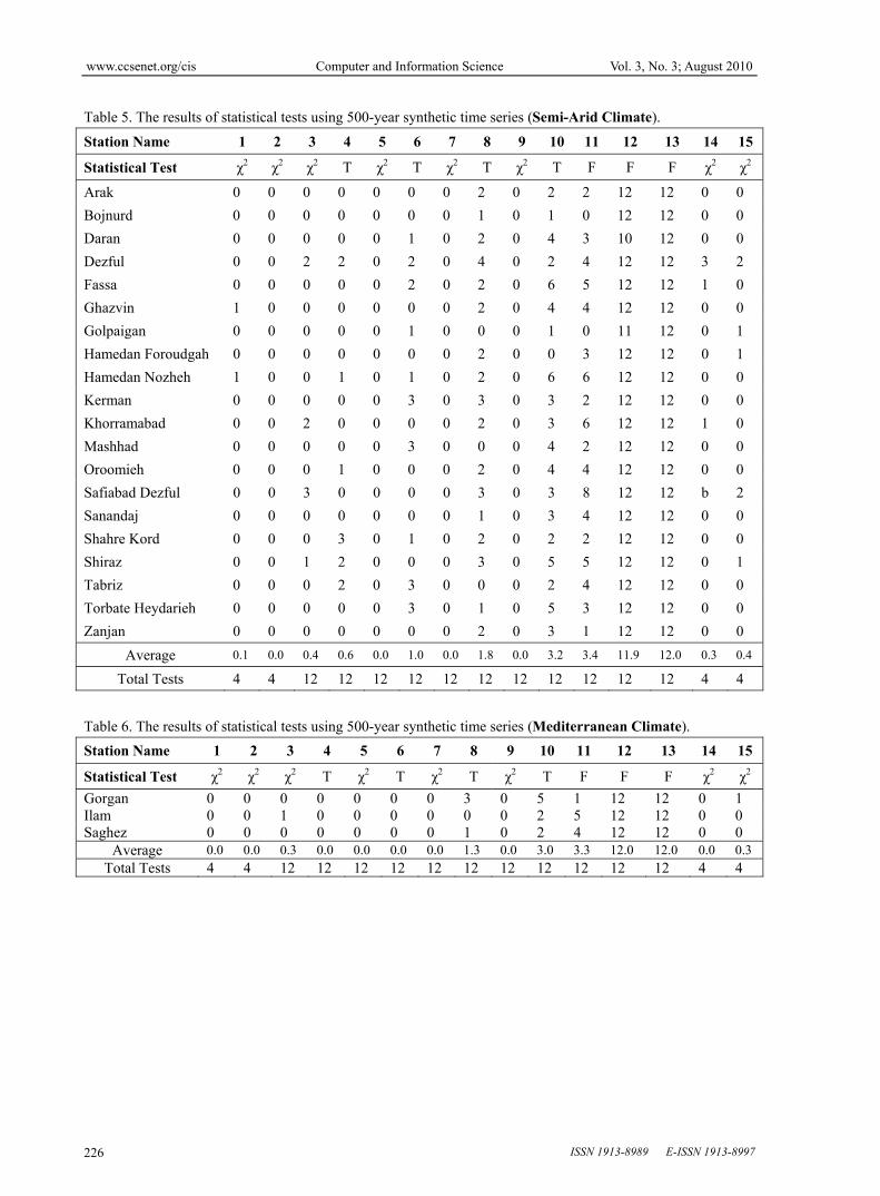
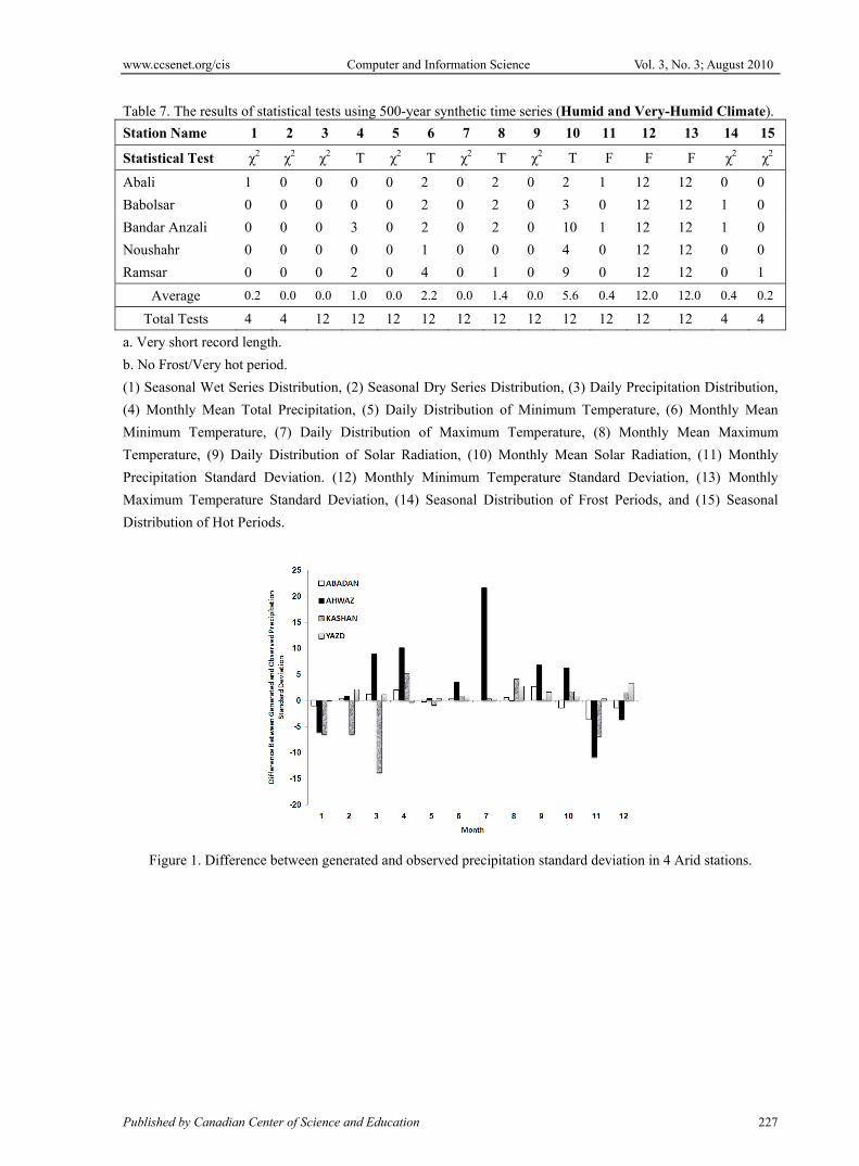
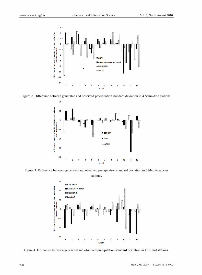
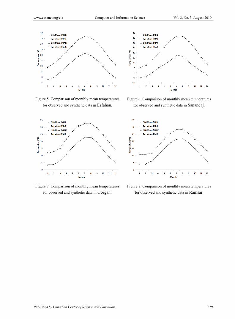
of observed data over a very long time period. Each test produces a p-value which measures the probability that both sets of data come from the same distribution (i.e. that there is no difference between the ‘true’ and synthetic climate for that variable). Hence, a very low p-value means that the synthetic climate is unlikely to be the same as the ‘true’ climate and so the generator is probably behaving poorly. Such tests cannot prove that the distributions are the same, and indeed the simplified nature of the generators means that there must be at least a small difference. A large p-value indicates that the differences are small enough that there is insufficient evidence to reject the null hypothesis. The required closeness of the synthetic and observed data depends upon the application in which the synthetic data are to be used. 3. Results and Discussion The number of tests that gave a p-value of less than 0.01 (i.e. a very significant result at the 99% confidence level) are shown in Tables 4 through 7 for different climates. A large number of such values mean that the model had a poor performance. The results for each variable are discussed below. The results of Humid and Very-Humid climates were combined because of their fewer station counts. 3.1 Wet and dry series LARS-WG simulates wet and dry series directly using semi-empirical distributions. The direct empirical approach of LARS-WG means that it is not surprising that it models the distributions well. As it can been seen from the Tables 4 to 7, the number of failed tests (very significant results) for Seasonal Wet Series Distribution (column 1) were, in average, 0.6, 0.1, 0.0, 0.2 and for Seasonal Dry Series Distribution (column 2) were, in average, 0.1, 0.0, 0.0 and 0.0 (out of 4) for Arid, Semi-Arid, Mediterranean, Humid (and Very-Humid) climates, respectively. It can be concluded that the LARS-WG model could model wet series better in humid stations compared with arid stations. 3.2 Precipitation Precipitation was tested in 3 different ways by comparing: 1) the daily rainfall distributions for each month of the year using a χ2 test (column 3), 2) the monthly means using the t-test (column 4), and 3) the monthly variances using the F-test (column 11). From Tables 4 to 7, the average number of failed tests (very significant results) for the daily distribution (χ2 test) were, in average, 1.6, 0.4, 0.3, 0.0 (out of 12), for the monthly means (t-test) were 0.4, 0.6, 0.0 and 1.0 (out of 12) and for the monthly variance (F-test) were 3.2, 3.4, 3.3 and 0.4 (out of 12) for Arid, Semi-Arid, Mediterranean, Humid (and Very-Humid) climates, respectively. From these numbers, it can be noted that the model is more capable in simulating the monthly means in comparison to the daily distribution of each month and the monthly variances. Also, it is more accurate in Humid (and Very-Humid) climates. The results for the inter-annual variances of monthly mean precipitation vary considerably from site to site from a total of no significant value at Ramsar to a total of 8 at Kermanshah. The major synthetic data tendency is to have a lower inter-annual variance than the observed data, and the main reason for this is probably that the model treats daily precipitation as independent events from the given monthly distribution (Semenov et al., 1998). From Figures 1 through 4, it can be seen that the model tends to overestimate, to some extent, the monthly standard deviation of total precipitation in arid regions, but to underestimate in Semi-Arid, Mediterranean and especially in Humid and Very-Humid regions. 3.3 Minimum and Maximum temperature LARS-WG reproduced the monthly means and daily distribution of maximum and minimum temperature well for all sites (column 5 to 8), but gave very poor results for the monthly variances (column 12 and 13). The generator tends to underestimate the annual variance in monthly means. From Tables 4 to 7, it can be seen that no significant result have been obtained for the minimum and maximum temperature daily distributions (Figures 5 to 8). Also, the average number of significant results for the monthly means ranged between 1.3 and 2.2 and is less in Mediterranean and Semi-Arid climates compared to other climates. 3.4 Solar radiation The model performs very well in terms of the daily distribution (column 9) and not so good in terms of the monthly mean solar radiation (column 10). The number of significant results for the mean values ranged from 3 (Mediterranean) to 5.6 (Humid and Very-Humid) in average. As for temperature, the generator tends to underestimate the inter-annual (monthly) variance. The fundamental assumption of weather generators is that the climate is stationary (Semenov et al., 1998) and so, before using the generators in such circumstances, the data should be de-trended.



3.5 Extreme temperature events The seasonal distributions of the length of spells with minimum temperatures below 0°C (frost) and maximum temperatures above 30°C (hot) for observed and synthetic data were compared using the χ2 test (columns 14 and 15). The performance LARS-WG varies from site to site. For 58 sites for LARS-WG, the number of failed tests does not exceed 2 (out of 8). For some sites, such as Kashan and Dezful, the number of failed tests was large. In terms of extreme temperature events, the quality of synthetic data is very important especially when it is to be used as an input data to an agricultural model. 4. Conclusion In this study, the performance of a popular weather generator model LARS-WG was examined in 65 weather/climatic stations across the country. The results showed that the model has different performance in diverse climates and also in different stations in a similar climate. The model performance in terms of the simulation of the mean values was very better than the monthly variance. In terms of Seasonal Wet/Dry Series Distribution, Daily Precipitation Distribution, and Monthly Precipitation Standard Deviation, the model had a better performance in Humid and Mediterranean regions in comparison with other climates. The performance of the model for Monthly Minimum Temperature Standard Deviation and Monthly Maximum Temperature Standard Deviation in all the climates was very poor and the model components needed a comprehensive revision. Again, In terms of Seasonal Distribution of Frost and Hot Periods, the model performed better (to some extent) in Humid and Mediterranean regions. Since the stations were not distributed uniformly through the different climates, the average values of the tables should be considered cautiously. Furthermore, it can be strongly recommended that the model should be evaluated for each station in which the model will be utilized. References Bailey, N. T. J. (1964). The Elements of Stochastic Processes, New York: Wiley. Doorenbos, J. & Pruit, W.O. (1984). Guidelines for predicting water requirements. FAO Irrigation and Drainage Paper No. 24, FAO, Rome, 1984. Downing, T.E., Harrison, P.A., Butterfield, R.E. & Lonsdale, K.G. (2000). Climate Change, Climatic Variability and Agriculture in Europe: An Integrated Assessment, Environmental Change Institute, University of Oxford. Harrison, P.A., Butterfield, R.E. & Downing, T.E. (1995). Climate Change and Agriculture in Europe: Assessment of Impacts and Adaptations. Environmental Change, Unit Research Report No. 9, Environmental Change Unit, University of Oxford. Hutchinson, M. (1995). Stochastic space-time weather models from ground-based data. Agric For Meteorol, 73, 237–265. Qian, B.D., Gameda, S., Hayhoe, H., De Jong, R. & Bootsma, A. (2004). Comparison of LARS-WG and AAFC-WG stochastic weather generators for diverse Canadian climates. Climate Research, 26, 175-191. Racsko, P., Szeidl, L. & Semenov, M.A. (1991). A serial approach to local stochastic weather models, Ecol Model, 57, 27–41. Richardson, C.W. (1981). Stochastic simulation of daily precipitation, temperature, and solar radiation. Wat Resour Res, 17, 182-190. Rietveld, M.R. (1978). A new method for the estimating the regression coefficients in the formula relating solar radiation to sunshine. Agricultural and Forest Meteorology, 19, 243-252. Semenov, M.A. & Barrow, E.M. (1997). Use of a stochastic weather generator in the development of climate change scenarios. Clim Change, 35, 397–414. Semenov, M.A. & Barrow, E.M. (2002). LARS-WG: A Stochastic Weather Generator for Use in Climate Impact Studies, Version 3.0, User’s Manual. Semenov, M.A. (2008). Simulation of extreme weather events by a stochastic weather generator. Climate Research, 35, 203-212. Semenov, M.A., Brooks, R.J., Barrow E.M. & Richardson, C.W. (1998). Comparison of the WGEN and LARS-WG stochastic weather generators for diverse climates, Clim. Res., 10 (2), 95–107. Semenov, M.A., Stratonovitch, P. (2009). The use of multi-model ensembles from global climate models for impact assessments of climate change. Climate Research, (in press).


ISSN 1913-8989 E-ISSN 1913-8997 222

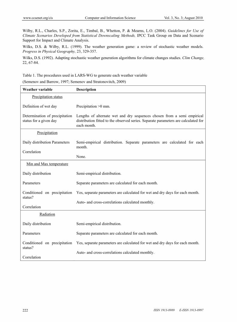
Wilby, R.L., Charles, S.P., Zorita, E., Timbal, B., Whetton, P. & Mearns, L.O. (2004). Guidelines for Use of Climate Scenarios Developed from Statistical Downscaling Methods, IPCC Task Group on Data and Scenario Support for Impact and Climate Analysis. Wilks, D.S. & Wilby, R.L. (1999). The weather generation game: a review of stochastic weather models. Progress in Physical Geography, 23, 329-357. Wilks, D.S. (1992). Adapting stochastic weather generation algorithms for climate changes studies. Clim Change, 22, 67-84. Table 1. The procedures used in LARS-WG to generate each weather variable (Semenov and Barrow, 1997; Semenov and Stratonovitch, 2009)

Weather variable Description

Precipitation status

Definition of wet day Determination of precipitation status for a given day

Precipitation >0 mm. Lengths of alternate wet and dry sequences chosen from a semi empirical distribution fitted to the observed series. Separate parameters are calculated for each month.

Precipitation

Daily distribution Parameters Correlation

Semi-empirical distribution. Separate parameters are calculated for each month. None.

Min and Max temperature

Daily distribution Parameters Conditioned on precipitation status? Correlation

Semi-empirical distribution. Separate parameters are calculated for each month. Yes, separate parameters are calculated for wet and dry days for each month. Auto- and cross-correlations calculated monthly.

Radiation

Daily distribution Parameters Conditioned on precipitation status? Correlation

Semi-empirical distribution. Separate parameters are calculated for each month. Yes, separate parameters are calculated for wet and dry days for each month. Auto- and cross-correlations calculated monthly.



Table 2. Characteristics of considered weather/climatic stations. Station Name Climate Lat.

(Deg) Long. (Deg)

Alt. (m)

Abadan Arid 48.25 30.37 6 Abadeh Arid 52.67 31.18 2030 Ahwaz Arid 48.67 31.33 22 Ardestan Arid 52.38 33.38 1252 Bam Arid 58.35 29.10 1066 Bandar Abbas Arid 56.37 27.22 9 Bandar Lengeh Arid 54.83 26.53 22 Birjand Arid 59.20 32.87 1491 Bushehr Arid 50.83 28.98 19 Bushehr (Coastal) Arid 50.82 28.90 8 Chahbahar Arid 60.62 25.28 8 Doushan Tappeh Arid 51.33 35.70 1209 Esfahan Arid 51.67 32.62 1550 Ghom Arid 50.85 34.70 877 Hasanabade Darab Arid 54.28 28.78 1098 Iranshahr Arid 60.70 27.20 591 Jask Arid 57.77 25.63 5 Kabootarabad Arid 51.85 32.52 1545 Karaj Arid 50.90 35.92 1312 Kashan Arid 51.45 33.98 982 Kermanshah Arid 47.15 34.35 1318 Khoor Biabanak Arid 55.08 33.78 845 Kish Arid 53.98 26.50 30 Lengeh (Coastal) Arid 54.90 26.57 6 Meimeh Arid 51.17 33.43 1980 Morchehkhort Arid 51.48 33.08 1669 Naein Arid 53.08 32.85 1549 Natanz Arid 51.90 33.53 1684 Sabzevar Arid 57.72 36.20 977 Semnan Arid 53.42 35.58 1127 Shahroud Arid 54.95 36.42 1345 Shargh Esfahan Arid 51.87 32.67 1543 Tabass Arid 56.92 33.60 711 Tehran (Mehrabad) Arid 51.32 35.68 1190 Yazd Arid 54.28 31.90 1237 Zabol Arid 61.48 31.03 489 Zahedan Arid 60.88 29.47 1370 Arak Semi-Arid 49.77 34.10 1708 Bojnurd Semi-Arid 57.32 37.47 1091 Daran Semi-Arid 50.37 32.97 2290 Dezful Semi-Arid 48.38 32.40 143 Fassa Semi-Arid 53.68 28.97 1288 Ghazvin Semi-Arid 50.05 36.25 1279 Golpaigan Semi-Arid 50.28 33.47 1870 Hamedan (Foroudgah) Semi-Arid 48.53 34.87 1741 Hamedan (Nozheh) Semi-Arid 48.72 35.20 1679 Kerman Semi-Arid 56.97 30.25 1753 Khorramabad Semi-Arid 48.28 33.43 1147 Mashhad Semi-Arid 59.63 36.27 999 Oroomieh Semi-Arid 45.05 37.67 1328 Safiabad Dezful Semi-Arid 48.42 32.27 82 Sanandaj Semi-Arid 47.00 35.33 1373 Shahrekord Semi-Arid 50.85 32.28 2048 Shiraz Semi-Arid 52.60 29.53 1484 Tabriz Semi-Arid 46.28 38.08 1361 Torbate Heydarieh Semi-Arid 59.22 35.27 1450 Zanjan Semi-Arid 48.48 36.68 1663 Gorgan Mediterranean 54.40 36.90 0 Ilam Mediterranean 46.43 33.63 1337 Saghez Mediterranean 46.27 36.25 1522 Abali Humid 51.88 35.75 2465 Babolsar Humid 52.65 36.72 -21 Bandar Anzali Very-Humid 49.47 37.47 -26 Noushahr Very-Humid 51.50 36.65 -20 Ramsar Very-Humid 50.67 36.90 -20


ISSN 1913-8989 E-ISSN 1913-8997 224

Table 3. Climatic classification according to De Martonne method. Climate I Range

Arid < 10 Semi-Arid 10 to 19.9 Mediterranean 20 to 23.9 Semi-Humid 24 to 27.9 Humid 28 to 34.9 Very-Humid > 35



Table 4 . The results of statistical tests using 500-year synthetic time series (Arid Climate). Station Name 1 2 3 4 5 6 7 8 9 10 11 12 13 14 15Statistical Test χ2 χ2 χ2 T χ2 T χ2 T χ2 T F F F χ2 χ2

Abadan 1 0 1 3 0 2 0 0 0 2 3 12 12 0 1 Abadeh 0 0 2 0 0 1 0 0 0 3 3 12 12 0 0 Ahwaz 2 1 4 0 0 2 0 1 0 4 7 12 12 1 1 Ardestan 1 0 1 0 0 1 0 2 0 3 2 12 12 1 0 Bam 0 0 2 0 0 2 0 0 0 5 4 12 12 1 0 Bandar Abbas 0 0 2 0 0 2 0 2 0 4 6 12 12 b 0 Bandar Lengeh 2 0 4 1 0 0 0 3 0 4 6 12 12 b 0 Birjand 0 0 0 3 0 4 0 2 0 7 4 12 12 0 0 Bushehr 2 0 2 1 0 1 0 2 0 4 5 12 12 0 1 Bushehr (Coastal) 1 0 3 1 0 1 0 0 0 0 4 11 12 b 0 Chahbahar 0 0 1 1 0 4 0 1 0 5 4 12 12 b 0 Doushan Tappeh 0 0 0 0 0 1 0 1 0 3 3 12 12 1 0 Esfahan 0 0 2 0 0 1 0 2 0 6 3 12 12 0 0 Ghom 1 0 0 0 0 3 0 3 0 3 1 12 12 1 0 Hasanabade Darab 0 0 0 0 0 0 0 0 0 4 0 7 11 0 0 Iranshahr 0 0 2 1 0 0 0 2 0 4 7 12 12 1 0 Jask 0 0 1 0 0 2 0 3 0 3 4 12 12 b 1 Kabootarabad 0 0 0 0 0 1 0 0 0 3 2 10 12 0 0 Karaj 1 0 1 0 0 0 0 2 0 3 0 7 7 0 2 Kashan 1 0 3 0 0 1 0 1 0 0 1 6 7 3 1 Kermanshah 0 0 0 0 0 0 0 1 0 7 8 12 12 0 0 Khoor Biabanak 0 0 4 0 0 1 0 3 0 1 2 12 12 0 0 Kish 0 0 5 1 0 1 0 4 0 2 7 12 12 b 1 Lengeh Coastal 2 0 3 1 0 3 0 0 0 0 a a a b 1 Meimeh 0 0 2 0 0 0 0 1 0 0 0 4 8 0 1 Morchehkhort 2 2 1 0 0 0 0 0 0 0 0 2 4 1 2 Naein 1 0 3 0 0 1 0 1 0 2 0 11 12 0 0 Natanz 0 0 0 0 0 1 0 1 0 0 1 12 12 1 1 Sabzevar 1 0 0 0 0 2 0 1 0 4 2 12 12 0 0 Semnan 0 0 0 1 0 1 0 1 0 6 1 12 12 0 0 Shahroud 0 0 0 0 0 2 0 2 0 3 1 12 12 0 0 Shargh Esfahan 0 0 1 0 0 0 0 0 0 4 4 12 12 0 0 Tabass 1 1 2 0 0 4 0 1 0 5 2 12 12 1 1 Tehran Mehrabad 1 0 0 2 0 2 0 2 0 5 5 12 12 0 0 Yazd 2 1 2 0 0 0 0 1 0 4 4 12 12 1 0 Zabol 1 0 4 0 0 3 0 2 0 6 4 12 12 1 0 Zahedan 0 0 1 0 0 3 0 4 0 8 4 12 12 0 0 Average 0.6 0.1 1.6 0.4 0.0 1.4 0.0 1.4 0.0 3.4 3.2 10.9 11.4 0.5 0.4Total Tests 4 4 12 12 12 12 12 12 12 12 12 12 12 4 4

a. Very short record length. b. No Frost/Very hot period. (1) Seasonal Wet Series Distribution, (2) Seasonal Dry Series Distribution, (3) Daily Precipitation Distribution, (4) Monthly Mean Total Precipitation, (5) Daily Distribution of Minimum Temperature, (6) Monthly Mean Minimum Temperature, (7) Daily Distribution of Maximum Temperature, (8) Monthly Mean Maximum Temperature, (9) Daily Distribution of Solar Radiation, (10) Monthly Mean Solar Radiation, (11) Monthly Precipitation Standard Deviation. (12) Monthly Minimum Temperature Standard Deviation, (13) Monthly Maximum Temperature Standard Deviation, (14) Seasonal Distribution of Frost Periods, and (15) Seasonal Distribution of Hot Periods.


ISSN 1913-8989 E-ISSN 1913-8997 226

Table 5 . The results of statistical tests using 500-year synthetic time series (Semi-Arid Climate).

Station Name 1 2 3 4 5 6 7 8 9 10 11 12 13 14 15

Statistical Test χ2 χ2 χ2 T χ2 T χ2 T χ2 T F F F χ2 χ2

Arak 0 0 0 0 0 0 0 2 0 2 2 12 12 0 0 Bojnurd 0 0 0 0 0 0 0 1 0 1 0 12 12 0 0 Daran 0 0 0 0 0 1 0 2 0 4 3 10 12 0 0 Dezful 0 0 2 2 0 2 0 4 0 2 4 12 12 3 2 Fassa 0 0 0 0 0 2 0 2 0 6 5 12 12 1 0 Ghazvin 1 0 0 0 0 0 0 2 0 4 4 12 12 0 0 Golpaigan 0 0 0 0 0 1 0 0 0 1 0 11 12 0 1 Hamedan Foroudgah 0 0 0 0 0 0 0 2 0 0 3 12 12 0 1 Hamedan Nozheh 1 0 0 1 0 1 0 2 0 6 6 12 12 0 0 Kerman 0 0 0 0 0 3 0 3 0 3 2 12 12 0 0 Khorramabad 0 0 2 0 0 0 0 2 0 3 6 12 12 1 0 Mashhad 0 0 0 0 0 3 0 0 0 4 2 12 12 0 0 Oroomieh 0 0 0 1 0 0 0 2 0 4 4 12 12 0 0 Safiabad Dezful 0 0 3 0 0 0 0 3 0 3 8 12 12 b 2 Sanandaj 0 0 0 0 0 0 0 1 0 3 4 12 12 0 0 Shahre Kord 0 0 0 3 0 1 0 2 0 2 2 12 12 0 0 Shiraz 0 0 1 2 0 0 0 3 0 5 5 12 12 0 1 Tabriz 0 0 0 2 0 3 0 0 0 2 4 12 12 0 0 Torbate Heydarieh 0 0 0 0 0 3 0 1 0 5 3 12 12 0 0 Zanjan 0 0 0 0 0 0 0 2 0 3 1 12 12 0 0

Average 0.1 0.0 0.4 0.6 0.0 1.0 0.0 1.8 0.0 3.2 3.4 11.9 12.0 0.3 0.4

Total Tests 4 4 12 12 12 12 12 12 12 12 12 12 12 4 4

Table 6 . The results of statistical tests using 500-year synthetic time series (Mediterranean Climate).

Station Name 1 2 3 4 5 6 7 8 9 10 11 12 13 14 15


Gorgan 0 0 0 0 0 0 0 3 0 5 1 12 12 0 1 Ilam 0 0 1 0 0 0 0 0 0 2 5 12 12 0 0 Saghez 0 0 0 0 0 0 0 1 0 2 4 12 12 0 0

Average 0.0 0.0 0.3 0.0 0.0 0.0 0.0 1.3 0.0 3.0 3.3 12.0 12.0 0.0 0.3Total Tests 4 4 12 12 12 12 12 12 12 12 12 12 12 4 4



Table 7 . The results of statistical tests using 500-year synthetic time series (Humid and Very-Humid Climate). Station Name 1 2 3 4 5 6 7 8 9 10 11 12 13 14 15


Abali 1 0 0 0 0 2 0 2 0 2 1 12 12 0 0 Babolsar 0 0 0 0 0 2 0 2 0 3 0 12 12 1 0 Bandar Anzali 0 0 0 3 0 2 0 2 0 10 1 12 12 1 0 Noushahr 0 0 0 0 0 1 0 0 0 4 0 12 12 0 0 Ramsar 0 0 0 2 0 4 0 1 0 9 0 12 12 0 1

Average 0.2 0.0 0.0 1.0 0.0 2.2 0.0 1.4 0.0 5.6 0.4 12.0 12.0 0.4 0.2

Total Tests 4 4 12 12 12 12 12 12 12 12 12 12 12 4 4 a. Very short record length. b. No Frost/Very hot period. (1) Seasonal Wet Series Distribution, (2) Seasonal Dry Series Distribution, (3) Daily Precipitation Distribution, (4) Monthly Mean Total Precipitation, (5) Daily Distribution of Minimum Temperature, (6) Monthly Mean Minimum Temperature, (7) Daily Distribution of Maximum Temperature, (8) Monthly Mean Maximum Temperature, (9) Daily Distribution of Solar Radiation, (10) Monthly Mean Solar Radiation, (11) Monthly Precipitation Standard Deviation. (12) Monthly Minimum Temperature Standard Deviation, (13) Monthly Maximum Temperature Standard Deviation, (14) Seasonal Distribution of Frost Periods, and (15) Seasonal Distribution of Hot Periods.

Figure 1. Difference between generated and observed precipitation standard deviation in 4 Arid stations.


ISSN 1913-8989 E-ISSN 1913-8997 228

Figure 2. Difference between generated and observed precipitation standard deviation in 4 Semi-Arid stations.

Figure 3. Difference between generated and observed precipitation standard deviation in 3 Mediterranean

stations.

Figure 4. Difference between generated and observed precipitation standard deviation in 4 Humid stations.



Figure 5. Comparison of monthly mean temperatures for observed and synthetic data in Esfahan.

Figure 6 . Comparison of monthly mean temperatures for observed and synthetic data in Sanandaj.

Figure 7 . Comparison of monthly mean temperatures for observed and synthetic data in Gorgan.

Figure 8 . Comparison of monthly mean temperatures for observed and synthetic data in Ramsar.

evaluation of a stochastic weather generator in different climates

Documents