estimation of multinomial logit models in r : the mlogit package

Estimation of multinomial logit models in R :

The mlogit Packages

Yves CroissantUniversite de la Reunion

Abstract

mlogit is a package for R which enables the estimation of the multinomial logitmodels with individual and/or alternative specific variables. The main extensions ofthe basic multinomial model (heteroscedastic, nested and random parameter models)are implemented.

Keywords:˜discrete choice models, maximum likelihood estimation, R, econometrics.

An introductory example

The logit model is useful when one tries to explain discrete choices, i.e. choices of oneamong several mutually exclusive alternatives1. There are many useful applications ofdiscrete choice modelling in different fields of applied econometrics, using individualdata, which may be :

revealed preferences data which means that the data are observed choices of indi-viduals for, say, a transport mode (car, plane and train for example),

stated preferences data ; in this case, individuals face a virtual situation of choice,for example the choice between three train tickets with different characteristics :

– A : a train ticket which costs 10 euros, for a trip of 30 minutes and one change,

– B : a train ticket which costs 20 euros, for a trip of 20 minutes and no change,

– C : a train ticket which costs 22 euros, for a trip of 22 minutes and one change.

Suppose that, in a transport mode situation, we can define an index of satisfaction Vjfor each alternative which depends linearly on cost (x) and time (z) :

V1 = α1 + βx1 + γz1

V2 = α2 + βx2 + γz2

V3 = α3 + βx3 + γz3

1For an extensive presentations of the logit model, see Train (2003) and Louiviere, Hensher, and Swait(2000)

Yves Croissant 2

In this case, the probability of choosing the alternative j is increasing with Vj . For sakeof estimation, one has to transform the satisfaction index, which can take any real valueso that it is restricted to the unit interval and can be interpreted as a probability. Themultinomial logit model is obtained by applying such a transformation to the Vjs. Morespecifically, we have :

P1 = eV1eV1+eV2+eV3

P2 = eV2eV1+eV2+eV3

P3 = eV3eV1+eV2+eV3

The two characteristics of probabilities are satisfied :

0 ≤ Pj ≤ 1 ∀i = 1, 2, 3,

∑3j=1 Pj = 1

Once fitted, a logit model is useful for predictions :

enter new values for the explanatory variables,

get

– at an individual level the probabilities of choice,

– at an aggregate level the market shares.

Consider, as an example, interurban trips between two towns (Lyon and Paris). Supposethat there are three modes (car, plane and train) and that the characteristics of the modesand the market shares are as follow :

price time share

car 50 4 20%plane 150 1 25%train 80 2 55%

With a sample of travellers, one can estimate the coefficients of the logit model, i.e. thecoefficients of time and price in the utility function.

The fitted model can then be used to predict the impact of some changes of the explana-tory variables on the market shares, for example :

the influence of train trips length on modal shares,

the influence of the arrival of low cost companies.

Yves Croissant 3

To get the predictions, one just has to change the values of train time or plane priceand compute the new probabilities, which can be interpreted at the aggregate level aspredicted market shares.

1. Data management and model description

1.1. Data management

mlogit is loaded using :

R> library("mlogit")

It comes with several data sets that we’ll use to illustrate the features of the library. Datasets used for multinomial logit estimation deals with some individuals, that make one or asequential choice of one alternative among a set of several alternatives. The determinantsof these choices are variables that can be alternative specific or purely individual specific.Such data have therefore a specific structure that can be characterised by three indexes:

the alternative,

the choice situation,

the individual.

the last one being only relevant if we have repeated observations for the same individual.

Data sets can have two different shapes :

a wide shape : in this case, there is one row for each choice situation,

a long shape : in this case, there is one row for each alternative and, therefore, asmany rows as there are alternatives for each choice situation.

This can be illustrated with three data sets.

Fishing is a revealed preferences data sets that deals with the choice of a fishingmode,

TravelMode (from the AER package) is also a revealed preferences data sets whichpresents the choice of individuals for a transport mode for inter-urban trips inAustralia,

Train is a stated preferences data sets for which individuals faces repeated virtualsituations of choice for train tickets.

Yves Croissant 4

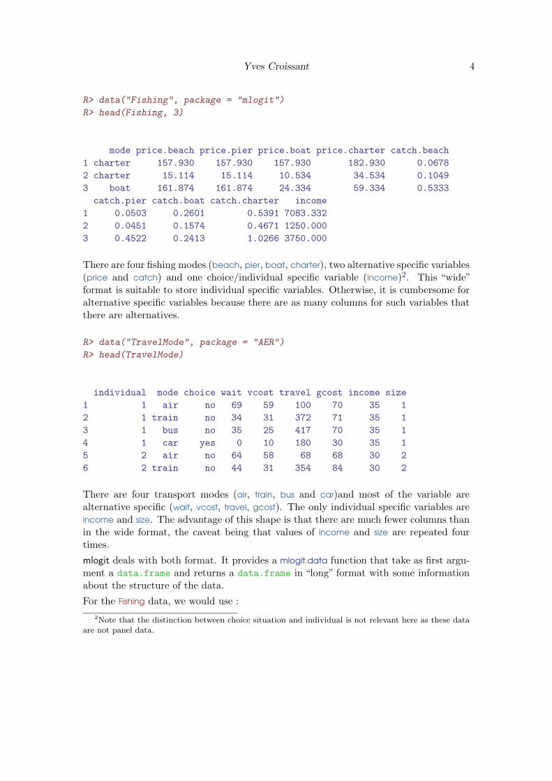
R> data("Fishing", package = "mlogit")

R> head(Fishing, 3)

mode price.beach price.pier price.boat price.charter catch.beach

1 charter 157.930 157.930 157.930 182.930 0.0678

2 charter 15.114 15.114 10.534 34.534 0.1049

3 boat 161.874 161.874 24.334 59.334 0.5333

catch.pier catch.boat catch.charter income

1 0.0503 0.2601 0.5391 7083.332

2 0.0451 0.1574 0.4671 1250.000

3 0.4522 0.2413 1.0266 3750.000

There are four fishing modes (beach, pier, boat, charter), two alternative specific variables(price and catch) and one choice/individual specific variable (income)2. This “wide”format is suitable to store individual specific variables. Otherwise, it is cumbersome foralternative specific variables because there are as many columns for such variables thatthere are alternatives.

R> data("TravelMode", package = "AER")

R> head(TravelMode)

individual mode choice wait vcost travel gcost income size

1 1 air no 69 59 100 70 35 1

2 1 train no 34 31 372 71 35 1

3 1 bus no 35 25 417 70 35 1

4 1 car yes 0 10 180 30 35 1

5 2 air no 64 58 68 68 30 2

6 2 train no 44 31 354 84 30 2

There are four transport modes (air, train, bus and car)and most of the variable arealternative specific (wait, vcost, travel, gcost). The only individual specific variables areincome and size. The advantage of this shape is that there are much fewer columns thanin the wide format, the caveat being that values of income and size are repeated fourtimes.

mlogit deals with both format. It provides a mlogit.data function that take as first argu-ment a data.frame and returns a data.frame in “long” format with some informationabout the structure of the data.

For the Fishing data, we would use :

2Note that the distinction between choice situation and individual is not relevant here as these dataare not panel data.

Yves Croissant 5

R> Fish <- mlogit.data(Fishing, shape = "wide", varying = 2:9, choice = "mode")

The mandatory arguments are choice, which is the variable that indicates the choicemade, the shape of the original data.frame and, if there are some alternative specificvariables, varying which is a numeric vector that indicates which columns containsalternative specific variables. This argument is then passed to reshape that coerced theoriginal data.frame in “long” format. Further arguments may be passed to reshape. Forexample, if the names of the variables are of the form var:alt, one can add sep = ’:’.

R> head(Fish, 5)

mode income alt price catch chid

1.beach FALSE 7083.332 beach 157.930 0.0678 1

1.boat FALSE 7083.332 boat 157.930 0.2601 1

1.charter TRUE 7083.332 charter 182.930 0.5391 1

1.pier FALSE 7083.332 pier 157.930 0.0503 1

2.beach FALSE 1250.000 beach 15.114 0.1049 2

The result is a data.frame in “long format” with one line for each alternative. The“choice” variable is now a logical variable and the individual specific variable (income)is repeated 4 times. An index attribute is added to the data, which contains the tworelevant index : chid is the choice index and alt index. This attribute is a data.frame

that can be extracted using the index function, which returns this data.frame.

R> head(index(Fish))

chid alt

1.beach 1 beach

1.boat 1 boat

1.charter 1 charter

1.pier 1 pier

2.beach 2 beach

2.boat 2 boat

For data in “long” format like TravelMode, the shape (here equal to long) and the choicearguments are still mandatory.

The information about the structure of the data can be explicitly indicated or, in part,guessed by the mlogit.data function. Here, we have 210 choice situations which areindicated by a variable called individual. The information about choice situations canalso be guessed from the fact that the data frame is balanced (every individual face4 alternatives) and that the rows are ordered first by choice situations and then byalternative.

Yves Croissant 6

Concerning the alternative, there are indicated by the mode variable and they can also beguessed thanks to the ordering of the rows and the fact that the data frame is balanced.

The first way to read correctly this data frame is to ignore completely the two indexvariables. In this case, the only supplementary argument to provide is the alt.levels

argument which is a character vector that contains the name of the alternatives :

R> TM <- mlogit.data(TravelMode, choice = "choice", shape = "long",

+ alt.levels = c("air", "train", "bus", "car"))

It is also possible to provide an argument alt.var which indicates the name of thevariable that contains the alternatives


+ alt.var = "mode")

The name of the variable that contains the information about the choice situations canbe indicated using the chid.var argument :


+ chid.var = "individual", alt.levels = c("air", "train", "bus",

+ "car"))

Both alternative and choice variable can be provided :


+ chid.var = "individual", alt.var = "mode")

and dropped from the data frame using the drop.index argument :


+ chid.var = "individual", alt.var = "mode", drop.index = TRUE)

R> head(TM)

choice wait vcost travel gcost income size

1.air FALSE 69 59 100 70 35 1

1.train FALSE 34 31 372 71 35 1

1.bus FALSE 35 25 417 70 35 1

1.car TRUE 0 10 180 30 35 1

2.air FALSE 64 58 68 68 30 2

2.train FALSE 44 31 354 84 30 2

The final example (Train) is in a “wide” format and contains panel data.

Yves Croissant 7

R> data("Train", package = "mlogit")

R> head(Train, 3)

id choiceid choice price1 time1 change1 comfort1 price2 time2 change2

1 1 1 choice1 2400 150 0 1 4000 150 0

2 1 2 choice1 2400 150 0 1 3200 130 0

3 1 3 choice1 2400 115 0 1 4000 115 0

comfort2

1 1

2 1

3 0

Each individual has responded to several (up to 16) scenario. To take this panel dimen-sion into account, one has to add an argument id which contains the individual variable.The index attribute has now a supplementary column, the individual index.

R> Tr <- mlogit.data(Train, shape = "wide", choice = "choice", varying = 4:11,

+ sep = "", alt.levels = c(1, 2), id = "id")

R> head(Tr, 3)

id choiceid choice alt price time change comfort chid

1.1 1 1 TRUE 1 2400 150 0 1 1

1.2 1 1 FALSE 2 4000 150 0 1 1

2.1 1 2 TRUE 1 2400 150 0 1 2

R> head(index(Tr), 3)

chid alt id

1.1 1 1 1

1.2 1 2 1

2.1 2 1 1

1.2. Model description

mlogit use the standard formula, data interface to describe the model to be estimated.However, standard formulas are not very practical for such models. More precisely, whileworking with multinomial logit models, one has to consider three kinds of variables :

alternative specific variables xij with a generic coefficient β,

Yves Croissant 8

individual specific variables zi with an alternative specific coefficients γj ,

alternative specific variables wij with an alternative specific coefficient δj .

The satisfaction index for the alternative j is then :

Vij = αj + βxij + γjzi + δjwij

Satisfaction being ordinal, only differences are relevant to modelize the choice for onealternative. This means that we’ll be interested in the difference between the satisfactionindex of two different alternatives j and k :

Vij − Vik = (αj − αk) + β(xij − xik) + (γj − γk)zi + (δjwij − δkwik)

It is clear from the previous expression that coefficients for individual specific variables(the intercept being one of those) should be alternative specific, otherwise they woulddisappear in the differentiation. Moreover, only differences of these coefficients are rel-evant and may be identified. For example, with three alternatives 1, 2 and 3, the threecoefficients γ1, γ2, γ3 associated to an individual specific variable cannot be identified,but only two linear combinations of them. Therefore, one has to make a choice of nor-malization and the most simple one is just to set γ1 = 0.

Coefficients for alternative specific variables may (or may not) be alternative specific.For example, transport time is alternative specific, but 10 mn in public transport maynot have the same impact on utility than 10 mn in a car. In this case, alternative specificcoefficients are relevant. Monetary time is also alternative specific, but in this case, onecan consider than 1 euro is 1 euro whatever it is spent in car or in public transports3.In this case, a generic coefficient is relevant.

A model with only individual specific variables is sometimes called a multinomial logitmodel, one with only alternative specific variables a conditional logit model and one withboth kind of variables a mixed logit model. This is seriously misleading : conditional logitmodel is also a logit model for longitudinal data in the statistical literature and mixedlogit is one of the names of a logit model with random parameters. Therefore, in whatfollow, we’ll use the name multinomial logit model for the model we’ve just describedwhatever the nature of the explanatory variables included in the model.

mlogit package provides objects of class mFormula which are extended model formulasand which are build upon Formula objects provided by the Formula package4.

To illustrate the use of mFormula objects, let’s use again the TravelMode data set. incomeand size (the size of the household) are individual specific variables. vcost (monetary cost)and travel (travel time) are alternative specific. We want to use a generic coefficient forthe former and alternative specific coefficients for the latter. This is done using themFormula function that build a three-parts formula :

3At least if the monetary cost of using car is correctly calculated.4See Zeileis and Croissant (2010) for a description of the Formula package.

Yves Croissant 9

R> f <- mFormula(choice ~ vcost | income + size | travel)

By default, an intercept is added to the model, it can be removed by using +0 or -1 inthe second part. Some parts may be omitted when there are no ambiguity. For example,the following couples of formulas are identical :

R> f2 <- mFormula(choice ~ vcost + travel | income + size)

R> f2 <- mFormula(choice ~ vcost + travel | income + size | 0)

R> f3 <- mFormula(choice ~ 0 | income | 0)

R> f3 <- mFormula(choice ~ 0 | income)

R> f4 <- mFormula(choice ~ vcost + travel)

R> f4 <- mFormula(choice ~ vcost + travel | 1)

R> f4 <- mFormula(choice ~ vcost + travel | 1 | 0)

Finally, we show below some formulas that describe models without intercepts (whichis generally hardly relevant)

R> f5 <- mFormula(choice ~ vcost | 0 | travel)

R> f6 <- mFormula(choice ~ vcost | income + 0 | travel)

R> f6 <- mFormula(choice ~ vcost | income - 1 | travel)

R> f7 <- mFormula(choice ~ 0 | income - 1 | travel)

model.matrix and model.frame methods are provided for mFormula objects. The for-mer is of particular interest, as illustrated in the following example :

R> f <- mFormula(choice ~ vcost | income | travel)

R> head(model.matrix(f, TM))

train:(intercept) bus:(intercept) car:(intercept) vcost train:income

1.air 0 0 0 59 0

1.train 1 0 0 31 35

1.bus 0 1 0 25 0

1.car 0 0 1 10 0

2.air 0 0 0 58 0

2.train 1 0 0 31 30

bus:income car:income air:travel train:travel bus:travel car:travel

1.air 0 0 100 0 0 0

1.train 0 0 0 372 0 0

1.bus 35 0 0 0 417 0

1.car 0 35 0 0 0 180

2.air 0 0 68 0 0 0

2.train 0 0 0 354 0 0

Yves Croissant 10

The model matrix contains J − 1 columns for every individual specific variables (incomeand the intercept), which means that the coefficient associated to the first alternative(air) is fixed to 0.

It contains only one column for vcost because we want a generic coefficient for thisvariable.

It contains J columns for travel, because it is an alternative specific variable for whichwe want an alternative specific coefficient.

2. Random utility model and the multinomial logit model

2.1. Random utility model

The individual must choose one alternative among J different and exclusive alternatives.A level of utility may be defined for each alternative and the individual is supposed tochoose the alternative with the highest level of utility. Utility is supposed to be the sumof two components5:

a systematic component, denoted Vj , which is a function of different observedvariables xj . For sake of simplicity, it will be supposed that this component is alinear combination of the observed explanatory variables : Vj = β>j xj ,

an unobserved component εj which, from the researcher point of view, can berepresented as a random variable. This error term includes the impact of all theunobserved variables which have an impact on the utility of choosing a specificalternative.

It is very important to understand that the utility and therefore the choice is purelydeterministic from the decision maker’s point of view. It is random form the searcher’spoint of view, because some of the determinants of the utility are unobserved, whichimplies that the choice can only be analyzed in terms of probabilities.

We have, for each alternative, the following utility levels :U1 = β>1 x1 + ε1 = V1 + ε1U2 = β>2 x2 + ε2 = V2 + ε2

......

UJ = β>J xJ + εJ = VJ + εJ

alternative l will be chosen if and only if ∀ j 6= l Ul > Uj which leads to the followingJ − 1 conditions :

5when possible, we’ll omit the individual index to simplify the notations.

Yves Croissant 11

Ul − U1 = (Vl − V1) + (εl − ε1) > 0Ul − U2 = (Vl − V2) + (εl − ε2) > 0

...Ul − UJ = (Vl − VJ) + (εl − εJ) > 0

As εj are not observed, choices can only be modeled in terms of probabilities from theresearcher point of view. The J − 1 conditions can be rewritten in terms of upper bondsfor the J − 1 remaining error terms :

ε1 < (Vl − V1) + εlε2 < (Vl − V2) + εl

...εJ < (Vl − VJ) + εl

The general expression of the probability of choosing alternative l is then :

(Pl | εl) = P(Ul > U1, . . . , Ul > UJ)

(Pl | εl) = F−l(ε1 < (Vl − V1) + εl, . . . , εJ < (Vl − VJ) + εl) (1)

where F−l is the multivariate distribution of J − 1 error terms (all the ε’s except εl).Note that this probability is conditional on the value of εl.

The unconditional probability (which depends only on β and on the value of the observedexplanatory variables is :

Pl =

∫(Pl | εl)fl(εl)dεl

Pl =

∫F−l((Vl − V1) + εl, . . . , (Vl − VJ) + εl)fl(εl)dεl (2)

where fl is the marginal density function of εl.

2.2. The distribution of the error terms

The multinomial logit model (McFadden 1974) is a special case of the model developedin the previous section. It relies on three hypothesis :

H1 : independence of errors

If the hypothesis of independence of errors is made, the univariate distribution of theerrors can be used :

Yves Croissant 12

P(Ul > U1) = F1(Vl − V1 + εl)P(Ul > U2) = F2(Vl − V2 + εl)

...P(Ul > UJ) = FJ(Vl − VJ + εl)

where Fj is the cumulative density of εj .

The conditional (1) and unconditional (2) probabilities are then :

(Pl | εl) =∏j 6=l

Fj(Vl − Vj + εl) (3)

Pl =

∫ ∏j 6=l

Fj(Vl − Vj + εl) fl(εl) dεl (4)

which means that the evaluation of only a one-dimensional integral is required to computethe probabilities.

H2 : Gumbel distribution

Each ε follows a Gumbel distribution :

f(z) =1

θe−

z−µθ e−e

− z−µθ

where µ is the location parameter and θ the scale parameter.

P (z < t) = F (t) =

∫ t

−∞

1

θe−

z−µθ e−e

− z−µθ dz = e−e

− t−µθ

The first two moments of the Gumbel distribution are E(z) = µ + θγ, where γ is the

Euler-Mascheroni constant (0.577) and V(z) = π2

6 θ2.

The mean of εjs is not identified if Vj contains an intercept. We can then, withoutloss of generality suppose that µj = 0 ∀j. Moreover, the overall scale of utility is notidentified. Therefore, only J−1 scale parameters may be identified, and a natural choiceof normalisation is to impose that one of the θj is equal to 1.

H3 identically distributed errors

As the location parameter is not identified for any error term, this hypothesis is essen-tially an homoscedasticity hypothesis, which means that the scale parameter of Gumbeldistribution is the same for all the alternatives. As one of them has been previously fixedto 1, we can therefore suppose that, without loss of generality, θj = 1 ∀j ∈ 1 . . . J in caseof homoscedasticity.

In this case, the conditional (3) and unconditional (4) probabilities further simplify to :

(Pl | εl) =∏j 6=l

F (Vl − Vj + εl) (5)

Yves Croissant 13

Pl =

∫ ∏j 6=l

F (Vl − Vj + εl) f(εl) dεl (6)

with F and f respectively the cumulative and the density of the standard Gumbeldistribution (i.e. with position and scale parameters equal to 0 and 1).

2.3. Computation of the probabilities

With these hypothesis on the distribution of the error terms, we can now show that theprobabilities have very simple, closed forms, which correspond to the logit transformationof the deterministic part of the utility.

Let’s start with the probability that the alternative l is better than one other alternativej. With hypothesis 2 and 3, it can be written :

P (εj < Vl − Vj + εl) = e−e−(Vl−Vj+εl)

(7)

With hypothesis 1, the probability of choosing l is then simply the product of probabil-ities (7) for all the alternatives except l :

(Pl | εl) =∏j 6=l

e−e−(Vl−Vj+εl)

(8)

The unconditional probability is the expected value of the previous expression withrespect to εl.

Pl =

∫ +∞

−∞(Pl | εl) e−εle−e

−εldεl =

∫ +∞

−∞

∏j 6=l


e−εle−e−εldεl (9)

We first begin by writing the preceding expression for all alternatives, including the lalternative.

Pl =

∫ +∞

−∞

∏j


e−εldεlPl =

∫ +∞

−∞e−∑

je−(Vl−Vj+εl)

e−εldεl =

∫ +∞

−∞e−e−εl

∑je−(Vl−Vj)

e−εldεl

We then use the following change of variable

t = e−εl ⇒ dt = −e−εldεl

The unconditional probability is therefore the following integral :

Yves Croissant 14

Pl =

∫ +∞

0e−t∑

je−(Vl−Vj)

dt

which has a closed form :

Pl =

−e−t∑

je−(Vl−Vj)∑

j e−(Vl−Vj)

+∞

0

=1∑

j e−(Vl−Vj)

and can be rewritten as the usual logit probability :

Pl =eVl∑j e

Vj(10)

2.4. IIA hypothesis

If we consider the probabilities of choice for two alternatives l and m, we have :

Pl =eVl∑j e

Vj

Pm =eVm∑j e

Vj

The ration of these two probabilities is :

PlPm

=eVl

eVm

This probability ratio for the two alternatives depends only on the characteristics ofthese two alternatives and not on those of other alternatives. This is called the IIAhypothesis (for independence of irrelevant alternatives).

If we use again the introductory example of urban trips between Lyon and Paris :

price time share

car 50 4 20%plane 150 1 20%train 80 2 60%

Suppose that, because of low cost companies arrival, the price of plane is now 100$. Themarket share of plane will increase (for example up to 60%). With a logit model, sharefor train / share for car is 3 before the price change, and will remain the same after theprice change. Therefore, the new predicted probabilities for car and train are 10 and30%.

Yves Croissant 15

The IIA hypothesis relies on the hypothesis of independence of the error terms. It is nota problem by itself and may even be considered as a useful feature for a well specifiedmodel. However, this hypothesis may be in practice violated if some important variablesare unobserved.

To see that, suppose that the utilities for two alternatives are :

Ui1 = α1 + β1zi + γxi1 + εi1

Ui2 = α2 + β2zi + γxi2 + εi2

with εi1 and εi2 uncorrelated. In this case, the logit model can be safely used, as thehypothesis of independence of the errors is satisfied.

If zi is unobserved, the estimated model is :

Ui1 = α1 + γxi1 + ηi1

Ui2 = α2 + γxi2 + ηi2

ηi1 = εi1 + β1zi

ηi2 = εi2 + β2zi

The error terms are now correlated because of the common influence of omitted variables.

2.5. Estimation

The coefficients of the multinomial logit model are estimated by full information maxi-mum likelihood.

The likelihood function

Let’s start with a very simple example. Suppose there are four individuals. For givenparameters and explanatory variables, we can calculate the probabilities. The likelihoodfor the sample is the probability associated to the sample :

choice Pi1 Pi2 Pi3 li1 1 0.5 0.2 0.3 0.52 3 0.2 0.4 0.4 0.43 2 0.6 0.1 0.3 0.14 2 0.3 0.6 0.1 0.6

With random sample the joint probability for the sample is simply the product of theprobabilities associated with every observation.

L = 0.5× 0.4× 0.1× 0.6

Yves Croissant 16

A compact expression of the probabilities that enter the likelihood function is obtainedby denoting yij a dummy variable which is equal to 1 if individual i made choice j and0 otherwise.

The probability of the choice made for one individual is then :

Pi =∏j

Pyijij

Or in log :

ln Pi =∑j

yij ln Pij

which leads to the log-likelihood function :

lnL =∑i

ln Pi =∑i

∑j

yij ln Pij

Properties of the maximum likelihood estimator

Under regularity conditions, the maximum likelihood estimator is consistent and has anasymptotic normal distribution. The variance of the estimator is :

V(θ) =

(E

(−∂

2 lnL

∂θ∂θ>(θ)

))−1

This expression can not be computed because it depends on the thrue values of theparameters. Three estimators have been proposed :

V1(θ) =(E(−∂2 lnL∂θ∂θ>

(θ)))−1

: this expression can be computed if the expected

value is computable,

V2(θ) =(−∂2 lnL∂θ∂θ>

(θ))−1

V3(θ) =∑ni=1

(∂ ln li∂θ (θ)

) (∂ ln li∂θ (θ)

)>: this expression is called the bhhh expres-

sion and doesn’t require the computation of the hessian.

Numerical optimization

We seek to calculate the maximum of a function f(x). This first order condition for amaximum is f ′(xo) = 0, but in general, there is no explicit solution for xo, which thenmust be numerically approximated. In this case, the following algorithm can be used :

1. Start with a value x called xt,

Yves Croissant 17

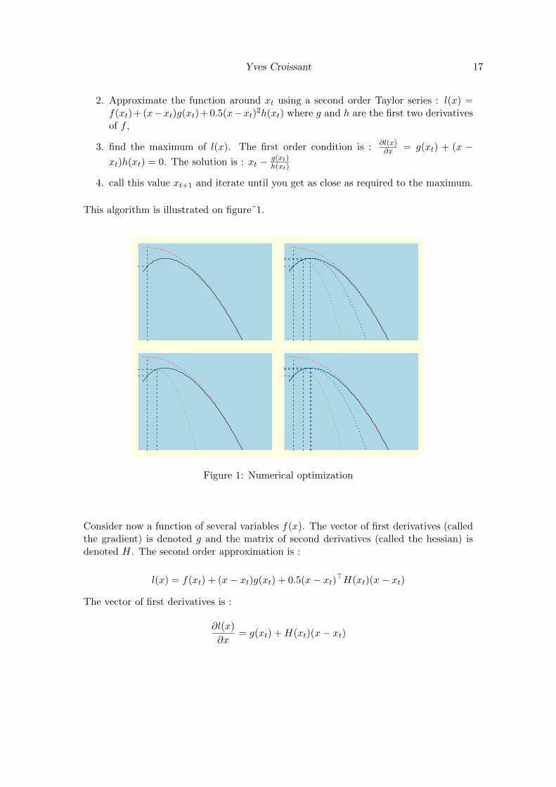
2. Approximate the function around xt using a second order Taylor series : l(x) =f(xt) + (x−xt)g(xt) + 0.5(x−xt)2h(xt) where g and h are the first two derivativesof f ,

3. find the maximum of l(x). The first order condition is : ∂l(x)∂x = g(xt) + (x −

xt)h(xt) = 0. The solution is : xt − g(xt)h(xt)

4. call this value xt+1 and iterate until you get as close as required to the maximum.

This algorithm is illustrated on figure˜1.

x1

x1 x2

x1 x2 x3

x1 x2 x3x4

Figure 1: Numerical optimization

Consider now a function of several variables f(x). The vector of first derivatives (calledthe gradient) is denoted g and the matrix of second derivatives (called the hessian) isdenoted H. The second order approximation is :

l(x) = f(xt) + (x− xt)g(xt) + 0.5(x− xt)>H(xt)(x− xt)

The vector of first derivatives is :

∂l(x)

∂x= g(xt) +H(xt)(x− xt)

Yves Croissant 18

x = xt −H(xt)−1g(xt)

Two kinds of routines are currently used for maximum likelihood estimation. The firstone can be called “Newton-like” methods. In this case, at each iteration, an estimation ofthe hessian is calculated, whether using the second derivatives of the function (Newton-Ralphson method) or using the outer product of the gradient (bhhh). This approach isvery powerful if the function is well-behaved, but it may perform poorly otherwise andfail after a few iterations.

The second one, called bfgs, updates at each iteration the estimation of the hessian. Itis often more robust and may performs well in cases where the first one doesn’t work.

Two optimization functions are included in core R: nlm which use the Newton-Ralphsonmethod and optim which use bfgs (among other methods). Recently, the maxLik package(Toomet and Henningsen 2010) provides a unified approach. With a unique interface,all the previously described methods are available.

The behavior of maxLik can be controlled by the user using in the estimation functionarguments like print.level (from 0-silent to 2-verbal), iterlim (the maximum numberof iterations), methods (the method used, one of nr, bhhh or bfgs) that are passed tomaxLik.

Gradient and Hessian for the logit model

For the multinomial logit model, the gradient and the hessian have very simple expres-sions.

∂ lnPij∂β

= xij −∑l

Pilxil

∂ lnL

∂β=∑i

∑j

(yij − Pij)xij

∂2 lnL

∂β∂β′=∑i

∑j

Pij

(xij −

∑l

Pilxil

)(xij −

∑l

Pilxil

)>

Moreover, the log-likelihood function is globally concave, which mean that there is aunique optimum which is the global maximum. In this case, the Newton-Ralphsonmethod is very efficient and the convergence is achieved after just a few iterations.

2.6. Interpretation

In a linear model, the coefficients can be directly considered as marginal effects of theexplanatory variables on the explained variable. This is not the case for the multinomialmodels. However, meaningful results can be obtained using relevant transformations ofthe coefficients.

Yves Croissant 19

Marginal effects

The marginal effects are the derivatives of the probabilities with respect to the explana-tory variables, which can be be individual-specific (zi) or alternative specific (xij) :

∂Pij∂zi

= Pij

(βj −

∑l

Pilβl

)

∂Pij∂xij

= γPij(1− Pij)

∂Pij∂xil

= −γPijPil

For an alternative-specific variable, the sign of the coefficient is directly inter-pretable. The marginal effect is obtained by multiplying the coefficient by theproduct of two probabilities which is at most 0.25. The rule of thumb is thereforeto divide the coefficient by 4 in order to have an upper bound of the marginaleffect.

For an individual specific variable, the sign of the coefficient is not necessarilythe sign of the coefficient. Actually, the sign of the marginal effect is given by(βj −

∑l Pilβl), which is positive if the coefficient for the j alternative is greater

than a weighted average of the coefficients for all the alternatives, the weightsbeing the probabilities of choosing the alternatives. In this case, the sign of themarginal effect can be established with no ambiguity only for the alternatives withthe lowest and the greatest coefficients.

Marginal rates of substitution

Coefficients are marginal utilities, which are not interpretable because utility is ordinal.However, ratios of coefficients are marginal rates of substitution, which are interpretable.For example, if the observable part of utility is : V = βo+β1x1+βx2+βx3, join variationsof x1 and x2 which ensure the same level of utility are such that : dV = β1dx1+β2dx2 = 0so that :

−dx2

dx1|dV=0=

β1

β2

For example, if x2 is transport cost (in euros), x1 transport time (in hours), β1 = 1.5and β2 = 0.2, β1

β2= 30 is the marginal rate of substitution of time in terms of euros and

the value of 30 means that to reduce the travel time of one hour, the individual is willingto pay at most 30 euros more.

Consumer’s surplus

Yves Croissant 20

Consumer’s surplus has a very simple expression with multinomial logit models. It wasfirst derived by Small and Rosen (1981).

The level of utility attained by an individual is Uj = Vj + εj , j being the alternativechosen. The expected utility, from the searcher’s point of view is then :

E(maxjUj)

where the expectation is taken on the values of all the error terms. If the marginal utilityof income (α) is known and constant, the expected surplus is simply E(maxj Uj)/α.

This expected surplus is a very simple expression in the context of the logit model, whichis called the “log-sum”. We’ll demonstrate this fact in the context of two alternatives.

With two alternatives, the values of ε1 and ε2 can be depicted in a plane. This planecontains all the possible combinations of (ε1, ε2). Some of them leads to the choice ofalternative 1 and the other to the choice of alternative 2. More precisely, alternative 1is chosen if ε2 ≤ V1 − V2 + ε1 and alternative 2 is chosen if ε1 ≤ V2 − V1 + ε2. The firstexpression is the equation of a straight line in the plan which delimits the choice for thetwo alternatives.

We can then write the expected utility as the sum of two terms E1 and E2, with :

E1 =

∫ ∞ε1=−∞

∫ V1−V2+ε1

−∞(V1 + ε1)f(ε1)f(ε2)dε1dε2

and

E2 =

∫ ∞ε2=−∞

∫ V2−V1+ε1

−∞(V2 + ε2)f(ε1)f(ε2)dε1dε2

with f(z) = exp (−e−z) the density of the Gumbell distribution.

We’ll derive the expression for E1, by symmetry we’ll guess the expression for E2 andwe’ll then obtain the expected utility by summing E1 and E2.

E1 =

∫ ∞ε1=−∞

(V1 + ε1)

(∫ V1−V2+ε1

−∞f(ε2)dε2

)f(ε1)dε1

The expression in brackets is the cumulative density of ε2. We then have :

E1 =

∫ ∞ε1=−∞

(V1 + ε1)e−e−(V1−V2)−ε1

f(ε1)dε1

E1 =

∫ ∞ε1=−∞

(V1 + ε1)e−ε1e−ae−ε1dε1

with a = 1 + e−(V1−V2) = eV1+eV2eV1

= 1P1

Yves Croissant 21

Let defines z | e−z = ae−ε1 ⇔ z = ε1 − ln a

We then have :

E1 =

∫ ∞ε1=−∞

(V1 + z + ln a)/ae−ze−e−zdz

E1 = (V1 + ln a)/a+ µ/a

where µ is the expected value of a random variable which follows a standard Gumbelldistribution, i.e. the Euler-Mascheroni constant.

E1 =ln(eV1 + eV2) + µ

(eV1 + eV2)/eV1=eV1 ln(eV1 + eV2) + eV1µ

eV1 + eV2

By symmetry,

E2 =eV2 ln(eV1 + eV2) + eV2µ

eV1 + eV2

And then :

E(U) = E1 + E2 = ln(eV1 + eV2) + µ

More generally, in presence of J alternatives, we have :

E(U) = lnJ∑j=1

eVj + µ

and the expected surplus is, with α the constant marginal utility of income˜:

E(U) =ln∑Jj=1 e

Vj + µ

α

2.7. Application

Train contains data about a stated preference survey in Netherlands. Users are asked tochoose between two train trips characterized by four attributes :

price : the price in cents of guilders,

time : travel time in minutes,

change : the number of changes,

comfort : the class of comfort, 0, 1 or 2, 0 being the most comfortable class.

Yves Croissant 22


R> Tr <- mlogit.data(Train, shape = "wide", choice = "choice", varying = 4:11,

+ sep = "", alt.levels = c(1, 2), id = "id")

We first convert price and time in more meaningful unities, hours and euros (1 guilder is2.20371 euros) :

R> Tr$price <- Tr$price/100 * 2.20371

R> Tr$time <- Tr$time/60

We then estimate the model : both alternatives being virtual train trips, it is relevantto use only generic coefficients and to remove the intercept :

R> ml.Train <- mlogit(choice ~ price + time + change + comfort |

+ -1, Tr)

R> summary(ml.Train)

Call:

mlogit(formula = choice ~ price + time + change + comfort | -1,

data = Tr, method = "nr", print.level = 0)

Frequencies of alternatives:

1 2

0.50324 0.49676

nr method

5 iterations, 0h:0m:0s

g'(-H)^-1g = 0.00014

successive fonction values within tolerance limits

Coefficients :

Estimate Std. Error t-value Pr(>|t|)

price -0.0673580 0.0033933 -19.8506 < 2.2e-16 ***

time -1.7205514 0.1603517 -10.7299 < 2.2e-16 ***

change -0.3263409 0.0594892 -5.4857 4.118e-08 ***

comfort -0.9457256 0.0649455 -14.5618 < 2.2e-16 ***

---

Signif. codes: 0 '***' 0.001 '**' 0.01 '*' 0.05 '.' 0.1 ' ' 1

Log-Likelihood: -1724.2

All the coefficients are highly significant and have the predicted negative sign (remindthan an increase in the variable comfort implies using a less comfortable class). The

Yves Croissant 23

coefficients are not directly interpretable, but dividing them by the price coefficient, weget monetary values :

R> coef(ml.Train)[-1]/coef(ml.Train)[1]

time change comfort

25.54337 4.84487 14.04028

We obtain the value of 26 euros for an hour of traveling, 5 euros for a change and 14euros to access a more comfortable class.

The second example use the Fishing data. It illustrates the multi-part formula interfaceto describe the model, and the fact that it is not necessary to transform the data setusing mlogit.data before the estimation, i.e. instead of using :


R> ml.Fish <- mlogit(mode ~ price | income | catch, Fish)

it is possible to use mlogit with the original data.frame and the relevant arguments thatwill be internally passed to mlogit.data :

R> ml.Fish <- mlogit(mode ~ price | income | catch, Fishing, shape = "wide",

+ varying = 2:9)

R> summary(ml.Fish)

Call:

mlogit(formula = mode ~ price | income | catch, data = Fishing,

shape = "wide", varying = 2:9, method = "nr", print.level = 0)


beach boat charter pier

0.11337 0.35364 0.38240 0.15059

nr method


g'(-H)^-1g = 2.54E-05


Coefficients :


boat:(intercept) 8.4184e-01 2.9996e-01 2.8065 0.0050080 **

charter:(intercept) 2.1549e+00 2.9746e-01 7.2443 4.348e-13 ***

Yves Croissant 24

pier:(intercept) 1.0430e+00 2.9535e-01 3.5315 0.0004132 ***

price -2.5281e-02 1.7551e-03 -14.4046 < 2.2e-16 ***

boat:income 5.5428e-05 5.2130e-05 1.0633 0.2876612

charter:income -7.2337e-05 5.2557e-05 -1.3764 0.1687088

pier:income -1.3550e-04 5.1172e-05 -2.6480 0.0080977 **

beach:catch 3.1177e+00 7.1305e-01 4.3724 1.229e-05 ***

boat:catch 2.5425e+00 5.2274e-01 4.8638 1.152e-06 ***

charter:catch 7.5949e-01 1.5420e-01 4.9254 8.417e-07 ***

pier:catch 2.8512e+00 7.7464e-01 3.6807 0.0002326 ***

---

Signif. codes: 0 '***' 0.001 '**' 0.01 '*' 0.05 '.' 0.1 ' ' 1


McFadden R^2: 0.19936

Likelihood ratio test : chisq = 597.16 (p.value = < 2.22e-16)

Several methods can be used to extract some results from the estimated model. fittedreturns the predicted probabilities for the outcome or for all the alternatives if outcome = FALSE.

R> head(fitted(ml.Fish))

1.beach 2.beach 3.beach 4.beach 5.beach 6.beach

0.3114002 0.4537956 0.4567631 0.3701758 0.4763721 0.4216448

R> head(fitted(ml.Fish, outcome = FALSE))

beach boat charter pier

[1,] 0.09299769 0.5011740 0.3114002 0.09442817

[2,] 0.09151070 0.2749292 0.4537956 0.17976449

[3,] 0.01410358 0.4567631 0.5125571 0.01657625

[4,] 0.17065868 0.1947959 0.2643696 0.37017585

[5,] 0.02858215 0.4763721 0.4543225 0.04072324

[6,] 0.01029791 0.5572463 0.4216448 0.01081103

Finally, two further arguments can be usefully used while using mlogit

reflevel indicates which alternative is the “reference” alternative, i.e. the one forwhich the coefficients are 0,

altsubset indicates a subset on which the estimation has to be performed ; in thiscase, only the lines that correspond to the selected alternatives are used and all theobservations which correspond to choices for unselected alternatives are removed :

Yves Croissant 25

R> mlogit(mode ~ price | income | catch, Fish, reflevel = "charter",

+ alt.subset = c("beach", "pier", "charter"))

Call:

mlogit(formula = mode ~ price | income | catch, data = Fish, alt.subset = c("beach", "pier", "charter"), reflevel = "charter", method = "nr", print.level = 0)

Coefficients:

beach:(intercept) pier:(intercept) price beach:income

-1.9952e+00 -9.4859e-01 -2.8343e-02 2.7184e-05

pier:income charter:catch beach:catch pier:catch

-1.0359e-04 1.1719e+00 3.2090e+00 2.8101e+00

2.8. The rank-ordered logit model

Sometimes, in stated-preference surveys, the respondents are asked to give the full rank oftheir preference for all the alternative, and not only the prefered alternative. The relevantmodel for this kind of data is the rank-ordered logit model, which can be estimated asa standard multinomial logit model if the data is reshaped correctly6

The ranking can be decomposed in a series of choices of the best alternative within adecreasing set of available alternatives. For example, with 4 alternatives, the probabilitythat the ranking would be 3-1-4-2 can be writen as follow :

alternative 3 is in the first position, the probability is then eβ>x3

eβ>x1+eβ

>x2+eβ>x3+eβ

>x4,

alternative 1 is in second position, the relevant probability is the logit probability

that 1 is the chosen alternative in the set of alternatives (1-2-4) : eβ>x1

eβ>x1+eβ

>x2+eβ>x4

,

alternative 4 is in third position, the relevant probability is the logit probability

that 4 is the chosen alternative in the set of alternatives (2-4) : eβ>x4

eβ>x2+eβ

>x4,

the probability of the full ranking is then simply the product of these 3 probabilities.

This model can therefore simply be fitted as a multinomial logit model ; the ranking forone individual amoung J alternatives is writen as J − 1 choices among J, J − 1, . . . , 2alternatives.

The estimation of the rank-ordered logit model is illustrated using the Game dataset˜Fok, Paap, and van Dijk (2010). Respondents are asked to rank 6 gaming plat-forms. The covariates are a dummy own which indicates whether a specific platformis curently owned, the age of the respondent (age) and the number of hours spent on

6see for example Beggs, Cardell, and Hausman (1981), Chapman and Staelin (1982) and Hausmanand Ruud (1987).

Yves Croissant 26

gaming per week (hours). The data set is available in wide (game) and long (game2)format. In wide format, the consists on J columns which indicate the ranking of eachalternative.

R> data("Game", package = "mlogit")

R> data("Game2", package = "mlogit")

R> head(Game, 2)

ch.Xbox ch.PlayStation ch.PSPortable ch.GameCube ch.GameBoy ch.PC own.Xbox

1 2 1 3 5 6 4 0

2 4 2 3 5 6 1 0

own.PlayStation own.PSPortable own.GameCube own.GameBoy own.PC age hours

1 1 0 0 0 1 33 2.00

2 1 0 0 0 1 19 3.25

R> head(Game2, 7)

age hours platform ch own chid

1 33 2.00 GameBoy 6 0 1

2 33 2.00 GameCube 5 0 1

3 33 2.00 PC 4 1 1

4 33 2.00 PlayStation 1 1 1

5 33 2.00 PSPortable 3 0 1

6 33 2.00 Xbox 2 0 1

7 19 3.25 GameBoy 6 0 2

R> nrow(Game)

[1] 91

R> nrow(Game2)

[1] 546

Note that Game contains 91 rows (there are 91 individuals) and that Game2 contains546 rows (91 individuals times 6 alternatives)

To use mlogit.data, the ranked should TRUE :

Yves Croissant 27

R> G <- mlogit.data(Game2, shape = "long", choice = "ch", alt.var = "platform",

+ ranked = TRUE)

R> G <- mlogit.data(Game, shape = "wide", choice = "ch", varying = 1:12,

+ ranked = TRUE)

R> head(G)

age hours alt own chid ch

1.GameBoy 33 2 GameBoy 0 1 FALSE

1.GameCube 33 2 GameCube 0 1 FALSE

1.PC 33 2 PC 1 1 FALSE

1.PlayStation 33 2 PlayStation 1 1 TRUE

1.PSPortable 33 2 PSPortable 0 1 FALSE

1.Xbox 33 2 Xbox 0 1 FALSE

R> nrow(G)

[1] 1820

Note that the choice variable is now a logical variable and that the number of row isnow 1820 (91 individuals ×(6 + 5 + 4 + 3 + 2) alternatives).

Using PC as the reference level, we can then reproduce the results of the original reference:

R> summary(mlogit(ch ~ own | hours + age, G, reflevel = "PC"))

Call:

mlogit(formula = ch ~ own | hours + age, data = G, reflevel = "PC",

method = "nr", print.level = 0)


PC GameBoy GameCube PlayStation PSPortable Xbox

0.17363 0.13846 0.13407 0.18462 0.17363 0.19560

nr method


g'(-H)^-1g = 6.74E-06


Coefficients :

Yves Croissant 28


GameBoy:(intercept) 1.570379 1.600251 0.9813 0.3264288

GameCube:(intercept) 1.404095 1.603483 0.8757 0.3812185

PlayStation:(intercept) 2.278506 1.606986 1.4179 0.1562270

PSPortable:(intercept) 2.583563 1.620778 1.5940 0.1109302

Xbox:(intercept) 2.733774 1.536098 1.7797 0.0751272 .

own 0.963367 0.190396 5.0598 4.197e-07 ***

GameBoy:hours -0.235611 0.052130 -4.5197 6.193e-06 ***

GameCube:hours -0.187070 0.051021 -3.6665 0.0002459 ***

PlayStation:hours -0.129196 0.044682 -2.8915 0.0038345 **

PSPortable:hours -0.233688 0.049412 -4.7294 2.252e-06 ***

Xbox:hours -0.173006 0.045698 -3.7858 0.0001532 ***

GameBoy:age -0.073587 0.078630 -0.9359 0.3493442

GameCube:age -0.067574 0.077631 -0.8704 0.3840547

PlayStation:age -0.067006 0.079365 -0.8443 0.3985154

PSPortable:age -0.088669 0.079421 -1.1164 0.2642304

Xbox:age -0.066659 0.075205 -0.8864 0.3754227

---

Signif. codes: 0 '***' 0.001 '**' 0.01 '*' 0.05 '.' 0.1 ' ' 1




3. Relaxing the iid hypothesis

With hypothesis 1 and 3, the error terms are iid (identically and independently dis-tributed), i.e. not correlated and homoscedastic. Extensions of the basic multinomiallogit model have been proposed by relaxing one of these two hypothesis while maintainingthe second hypothesis of Gumbell distribution.

3.1. The heteroskedastic logit model

The heteroskedastic logit model was proposed by Bhat (1995).

The probability that Ul > Uj is :

P (εj < Vl − Vj + εl) = e−e−

(Vl−Vj+εl)θj

which implies the following conditional and unconditional probabilities

(Pl | εl) =∏j 6=l

e−e−

(Vl−Vj+εl)θj

(11)

Yves Croissant 29

Pl =

∫ +∞

−∞

∏j 6=l

e−e− (Vl−Vj+εl)θj

1

θle− εlθl e−e

−εlθl dεl (12)

We then apply the following change of variable :

u = e− εlθl ⇒ du = − 1

θle− εlθl dεl

The unconditional probability (12) can then be rewritten :

Pl =

∫ +∞

0

∏j 6=l

e−e−Vl−Vj−θl lnuθj

e−udu =

∫ +∞

0

e−∑j 6=l e−Vl−Vj−θl lnu

θj

e−uduThere is no closed form for this integral but it can be written the following way :

Pl =

∫ +∞

0Gle−udu

with

Gl = e−Al Al =∑j 6=l

αj αj = e−Vl−Vj−θl lnu

θj

This one-dimensional integral can be efficiently computed using a Gauss quadraturemethod, and more precisely the Gauss-Laguerre quadrature method :

∫ +∞

0f(u)e−udu =

∑t

f(ut)wt

where ut and wt are respectively the nodes and the weights.

Pl =∑t

Gl(ut)wt

∂Gl∂βk

=∑j 6=l

αjθj

(xlk − xjk)Gl

∂Gl∂θl

= − lnu∑j 6=l

αjθjGl

∂Gl∂θj

= lnαjαjθjGl

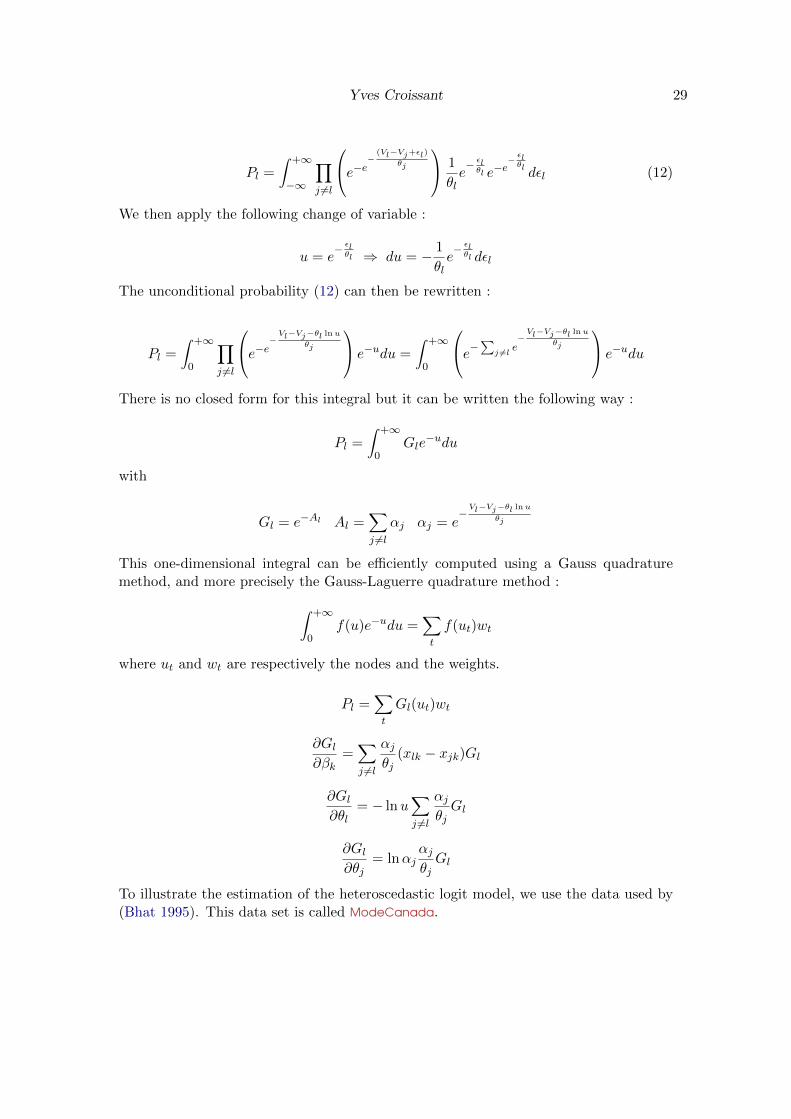
To illustrate the estimation of the heteroscedastic logit model, we use the data used by(Bhat 1995). This data set is called ModeCanada.

Yves Croissant 30

R> data("ModeCanada", package = "mlogit")

As done in the article, we first restrict the sample to the user who don’t choose the busand choose a mode among the four modes available (train, air, bus and car).

R> busUsers <- with(ModeCanada, case[choice == 1 & alt == "bus"])

R> Bhat <- subset(ModeCanada, !case %in% busUsers & alt != "bus" &

+ nchoice == 4)

R> Bhat$alt <- Bhat$alt[drop = TRUE]

R> Bhat <- mlogit.data(Bhat, shape = "long", chid.var = "case",

+ alt.var = "alt", choice = "choice", drop.index = TRUE)

This restricts the sample to 2769 users.

R> ml.MC <- mlogit(choice ~ freq + cost + ivt + ovt | urban + income,

+ Bhat, reflevel = "car")

R> hl.MC <- mlogit(choice ~ freq + cost + ivt + ovt | urban + income,

+ Bhat, reflevel = "car", heterosc = TRUE)

R> summary(hl.MC)

Call:

mlogit(formula = choice ~ freq + cost + ivt + ovt | urban + income,

data = Bhat, reflevel = "car", heterosc = TRUE)


car train air

0.45757 0.16721 0.37523

bfgs method


g'(-H)^-1g = 2.89E-07

gradient close to zero

Coefficients :


train:(intercept) 0.6783934 0.3327626 2.0387 0.041483 *

air:(intercept) 0.6567544 0.4681631 1.4028 0.160667

freq 0.0639247 0.0049168 13.0014 < 2.2e-16 ***

cost -0.0269615 0.0042831 -6.2948 3.078e-10 ***

ivt -0.0096808 0.0010539 -9.1859 < 2.2e-16 ***

ovt -0.0321655 0.0035930 -8.9523 < 2.2e-16 ***

train:urban 0.7971316 0.1207392 6.6021 4.054e-11 ***

Yves Croissant 31

air:urban 0.4454726 0.0821609 5.4220 5.895e-08 ***

train:income -0.0125979 0.0039942 -3.1541 0.001610 **

air:income 0.0188600 0.0032159 5.8646 4.503e-09 ***

sp.train 1.2371829 0.1104610 11.2002 < 2.2e-16 ***

sp.air 0.5403239 0.1118353 4.8314 1.356e-06 ***

---

Signif. codes: 0 '***' 0.001 '**' 0.01 '*' 0.05 '.' 0.1 ' ' 1



Likelihood ratio test : chisq = 1998 (p.value = < 2.22e-16)

The results obtained by Bhat (1995) can’t be exactly reproduced because he uses someweights that are not available in the data set. However, we obtain very close values forthe two estimated scale parameters for the train sp.train and for the air mode sp.air.

The second example uses the TravelMode data set and reproduces the first column oftable 23.28 page 855 of Greene (2008).


R> TravelMode <- mlogit.data(TravelMode, choice = "choice", shape = "long",

+ alt.var = "mode", chid.var = "individual")

R> TravelMode$avinc <- with(TravelMode, (mode == "air") * income)

R> ml.TM <- mlogit(choice ~ wait + gcost + avinc, TravelMode, reflevel = "car")

R> hl.TM <- mlogit(choice ~ wait + gcost + avinc, TravelMode, reflevel = "car",

+ heterosc = TRUE)

R> summary(hl.TM)

Call:

mlogit(formula = choice ~ wait + gcost + avinc, data = TravelMode,

reflevel = "car", heterosc = TRUE)


car air train bus

0.28095 0.27619 0.30000 0.14286

bfgs method


g'(-H)^-1g = 3.77E-07


Coefficients :


Yves Croissant 32

air:(intercept) 7.832450 10.950706 0.7152 0.4745

train:(intercept) 7.171867 9.135295 0.7851 0.4324

bus:(intercept) 6.865775 8.829608 0.7776 0.4368

wait -0.196843 0.288274 -0.6828 0.4947

gcost -0.051562 0.069444 -0.7425 0.4578

avinc 0.040253 0.060680 0.6634 0.5071

sp.air 4.024020 5.977821 0.6732 0.5008

sp.train 3.854208 6.220456 0.6196 0.5355

sp.bus 1.648749 2.826916 0.5832 0.5597




Note that the ranking of the scale parameters differs from the previous example. Inparticular, the error of the air utility has the largest variance as it has the smallest onein the previous example.

The standard deviations print at the end of table 23.28 are obtained by multiplying thescale parameters by π/

√6 :

R> c(coef(hl.TM)[7:9], sp.car = 1) * pi/sqrt(6)

sp.air sp.train sp.bus sp.car

5.161007 4.943214 2.114603 1.282550

Note that the standard deviations of the estimated scale parameters are very high, whichmeans that they are poorly identified.

3.2. The nested logit model

The nested logit model was first proposed by McFadden (1978). It is a generalizationof the multinomial logit model that is based on the idea that some alternatives maybe joined in several groups (called nests). The error terms may then present somecorrelation in the same nest, whereas error terms of different nests are still uncorrelated.

We suppose that the alternatives can be put into M different nests. This implies thefollowing multivariate distribution for the error terms.

exp

− M∑m=1

∑j∈Bm

e−εj/λm

λm

The marginal distributions of the εs are still univariate extreme value, but there is nowsome correlation within nests. 1−λm is a measure of the correlation, i.e. λm = 1 implies

Yves Croissant 33

no correlation. It can then be shown that the probability of choosing alternative j thatbelongs to the nest l is :

Pj =eVj/λl

(∑k∈Bl e

Vk/λl)λl−1

∑Mm=1

(∑k∈Bm e

Vk/λm)λm

and that this model is compatible with the random utility maximisation hypothesis ifall the nest elasticities are in the 0− 1 interval.

Let us now write the deterministic part of the utility of the alternative j as the sum oftwo terms : the first one being specific to the alternative and the second one to the nestit belongs to :

Vj = Zj +Wl

We can then rewrite the probabilities as follow :

Pj =e(Zj+Wl)/λl∑

k∈Bl e(Zk+Wl)/λl

×

(∑k∈Bl e

(Zk+Wl)/λl)λl

∑Mm=1

(∑k∈Bm e

(Zk+Wm)/λm)λm

Pj =eZj/λl∑

k∈Bl eZk/λl

×

(∑k∈Bl e

(Zk+Wl)/λl)λl

∑Mm=1

(∑k∈Bm e

(Zk+Wm)/λm)λm

∑k∈Bl

e(Zk+Wl)/λl

λl =

eWl/λl∑k∈Bl

eZk/λl

λl = eWl+λlIl

with Il = ln∑k∈Bl e

Zk/λl which is often called the inclusive value or the inclusive utility.

We then can write the probability of choosing alternative j as :

Pj =eZj/λl∑

k∈Bl eZk/λl

× eWl+λlIl∑Mm=1 e

Wm+λmIm

The first term Pj|l is the conditional probability of choosing alternative j if the nest lis chosen. It is often referred as the lower model. The second term Pl is the marginalprobability of choosing the nest l and is referred as the upper model. Wm + λmIm canbe interpreted as the expected utility of choosing the best alternative of the nest m,Wm being the expected utility of choosing an alternative in this nest (whatever thisalternative is) and λmIm being the expected extra utility he receives by being able tochoose the best alternative in the nest. The inclusive values links the two models. It isthen straightforward to show that IIA applies within nests, but not for two alternativesin different nests.

A slightly different version of the nested logit model (Daly 1987) is often used, but isnot compatible with the random utility maximization hypothesis. Its difference with the

Yves Croissant 34

previous expression is that the deterministic parts of the utility for each alternative isnot divided by the nest elasticity :

Pj =eVj

(∑k∈Bl e

Vk)λl−1

∑Mm=1

(∑k∈Bm e

Vk)λm

The differences between the two versions have been discussed in Koppelman and Wen(1998), Heiss (2002) and Hensher and Greene (2002).

The gradient is, for the first version of the model and denoting Nm =∑k∈Bm e

Vk/λm :

∂ lnPj∂β =

xjλl

+ λl−1λl

1Nl

∑k∈Bl e

Vk/λlxk − 1∑mNλmm

∑mN

λm−1m

∑k∈Bm e

Vk/λmxk∂ lnPj∂λl

= −Vjλ2l

+ lnNl − λl−1λ2l

1Nl

∑k∈Bl Vke

Vk/λl

− Nλll∑

mNλmm

(lnNl − 1

λlNl

∑k∈Bl Vke

Vk/λl)

∂ lnPj∂λm

= − Nλmm∑

mNλmm

(lnNm − 1

λmNm

∑k∈Bm Vke

Vk/λm)

Denoting Pj|l = eVj/λlNl

the conditional probability of choosing alternative j if nest l is

chosen, Pl =Nλll∑

mNλmm

the probability of choosing nest l, xl =∑k∈Bl Pk|lxk the weight

average value of x in nest l, x =∑Mm=1 Pmxm the weight average of x for all the nests

and Vl =∑k∈Bl Pk|lVk∂ lnPj∂β = 1

λl[xj − (1− λl)xl]− x

∂ lnPj∂λl

= − 1λ2l

[Vj − λ2

l lnNl − (1− λl)Vl]− Pl

λ2l

[λ2l lnNl − λlVl

]∂ lnPj∂λm

= Pmλm

[Vm − λm lnNm

]

∂ lnPj∂β =

xj−(1−λl)xl+λlxλl

∂ lnPj∂λl

= −Vj−λl(1−Pl)λl lnNl+(1−λl(1−Pl))Vlλ2l

∂ lnPj∂λm

= Pmλm

[Vm − λm lnNm

]For the unscaled version, the gradient is :

∂ lnPj∂β = xj − (1− λl)xl −

∑m λmPmxm

∂ lnPj∂λl

= (1− Pl) lnNl∂ lnPj∂λm

= −Pm lnNm

Until now, we have supposed that every alternative belongs to one and only one nest.If some alternatives belong to several nests, we get an overlapping nests model. In thiscase, the notations should be slightly modified :

Yves Croissant 35

Pj =

∑l|j∈Bl e

Vj/λlNλl−1l∑

mNλmm

Pj =∑l|j∈Bl

eVj/λl

Nl

Nλll∑

mNλmm

=∑l|j∈Bl

Pj|lPl

∂ lnPj∂β =

∑l|j∈Bl

Pj|lPlPj

xj−(1−λl)xl+λlxλl

∂ lnPj∂λl

= −Pj|lPlPj

Vj−λl(1−Pj/Pj|l)λl lnNl+(1−λl(1−Pj/Pj|l))Vlλ2l

∂ lnPj∂λm

= Pmλm

[Vm − λm lnNm

]For the unscaled version of the model, the gradient is :

∂ lnPj∂β =

∑l|j∈Bl

Pj|lPlPj

(xj − (1− λl)xl)−∑m λmPmxm

∂ lnPj∂λl

= Pl(PjlPj− 1

)lnNl

∂ lnPj∂λm

= −Pm lnNm

We illustrate the estimation of the unscaled nested logit model with an example used in(Greene 2008). The dataset, called TravelMode has already been used. Four transportmodes are available and two nests are considered :

the ground nest with bus, train and car modes,

the fly nest with the air modes.

Note that the second nest is a “degenerate” nest, which means that it contains only onealternative. In this case, the nest elasticity is difficult to interpret, as it is related tothe degree of correlation of the alternatives within the nests and that there is only onealternative in this nest. This parameter can only be identified in a very special case :the use of the unscaled version of the nested logit model with generic variable. This isexactly the situation considered by (Greene 2008) and presented in the table 21.11 p.730.


R> TravelMode <- mlogit.data(TravelMode, choice = "choice", shape = "long",

+ alt.var = "mode", chid.var = "individual")

R> TravelMode$avinc <- with(TravelMode, (mode == "air") * income)

R> nl.TM <- mlogit(choice ~ wait + gcost + avinc, TravelMode, reflevel = "car",

+ nests = list(fly = "air", ground = c("train", "bus", "car")),

+ unscaled = TRUE)

R> summary(nl.TM)

Yves Croissant 36

Call:

mlogit(formula = choice ~ wait + gcost + avinc, data = TravelMode,

reflevel = "car", nests = list(fly = "air", ground = c("train",

"bus", "car")), unscaled = TRUE)


car air train bus

0.28095 0.27619 0.30000 0.14286

bfgs method


g'(-H)^-1g = 1.02E-07


Coefficients :


air:(intercept) 6.042373 1.331325 4.5386 5.662e-06 ***

train:(intercept) 5.064620 0.676010 7.4919 6.795e-14 ***

bus:(intercept) 4.096325 0.628870 6.5138 7.328e-11 ***

wait -0.112618 0.011826 -9.5232 < 2.2e-16 ***

gcost -0.031588 0.007434 -4.2491 2.147e-05 ***

avinc 0.026162 0.019842 1.3185 0.18732

iv.fly 0.586009 0.113056 5.1833 2.180e-07 ***

iv.ground 0.388962 0.157904 2.4633 0.01377 *

---

Signif. codes: 0 '***' 0.001 '**' 0.01 '*' 0.05 '.' 0.1 ' ' 1




The second example deals with a choice of a heating mode. The data set is called HC.There are seven alternatives, four of them provide also cooling : gaz central with coolinggcc, electric central with cooling ecc, electric room with cooling erc and heat pumpwith cooling hpc ; the other three provide only heating, these are electric central ec,electric room er and gaz central gc.

R> data("HC", package = "mlogit")

R> HC <- mlogit.data(HC, varying = c(2:8, 10:16), choice = "depvar",

+ shape = "wide")

R> head(HC)

Yves Croissant 37

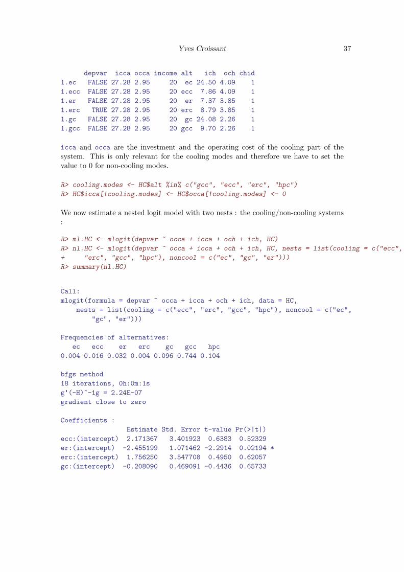
depvar icca occa income alt ich och chid

1.ec FALSE 27.28 2.95 20 ec 24.50 4.09 1

1.ecc FALSE 27.28 2.95 20 ecc 7.86 4.09 1

1.er FALSE 27.28 2.95 20 er 7.37 3.85 1

1.erc TRUE 27.28 2.95 20 erc 8.79 3.85 1

1.gc FALSE 27.28 2.95 20 gc 24.08 2.26 1

1.gcc FALSE 27.28 2.95 20 gcc 9.70 2.26 1

icca and occa are the investment and the operating cost of the cooling part of thesystem. This is only relevant for the cooling modes and therefore we have to set thevalue to 0 for non-cooling modes.

R> cooling.modes <- HC$alt %in% c("gcc", "ecc", "erc", "hpc")

R> HC$icca[!cooling.modes] <- HC$occa[!cooling.modes] <- 0

We now estimate a nested logit model with two nests : the cooling/non-cooling systems:

R> ml.HC <- mlogit(depvar ~ occa + icca + och + ich, HC)

R> nl.HC <- mlogit(depvar ~ occa + icca + och + ich, HC, nests = list(cooling = c("ecc",

+ "erc", "gcc", "hpc"), noncool = c("ec", "gc", "er")))

R> summary(nl.HC)

Call:

mlogit(formula = depvar ~ occa + icca + och + ich, data = HC,

nests = list(cooling = c("ecc", "erc", "gcc", "hpc"), noncool = c("ec",

"gc", "er")))


ec ecc er erc gc gcc hpc

0.004 0.016 0.032 0.004 0.096 0.744 0.104

bfgs method


g'(-H)^-1g = 2.24E-07


Coefficients :


ecc:(intercept) 2.171367 3.401923 0.6383 0.52329

er:(intercept) -2.455199 1.071462 -2.2914 0.02194 *

erc:(intercept) 1.756250 3.547708 0.4950 0.62057

gc:(intercept) -0.208090 0.469091 -0.4436 0.65733

Yves Croissant 38

gcc:(intercept) 2.234177 3.383645 0.6603 0.50907

hpc:(intercept) 1.272654 3.618232 0.3517 0.72504

occa -0.966387 0.708161 -1.3646 0.17237

icca -0.051249 0.081461 -0.6291 0.52927

och -0.868681 0.445484 -1.9500 0.05118 .

ich -0.205005 0.090851 -2.2565 0.02404 *

iv.cooling 0.333827 0.172073 1.9400 0.05238 .

iv.noncool 0.328934 0.212062 1.5511 0.12087

---

Signif. codes: 0 '***' 0.001 '**' 0.01 '*' 0.05 '.' 0.1 ' ' 1



Likelihood ratio test : chisq = 74.354 (p.value = 5.2125e-14)

The two nest elasticities are about 0.3, which implies a correlation of 0.7, which is quitehigh. The two nest elasticities are very close to each other, and it is possible to enforcethe equality by updating the model with the argument un.nest.el set to TRUE.

R> nl.HC.u <- update(nl.HC, un.nest.el = TRUE)

3.3. The general extreme value model

Derivation of the general extreme value model

McFadden (1978) developed a general model that suppose that the join distribution ofthe error terms follow a a multivariate extreme value distribution. Let G be a functionwith J arguments yj ≥ 0. G has the following characteristics :

i) it is non negative G(y1, . . . , yJ) ≥ 0 ∀j ,

ii) it is homogeneous of degree 1 in all its arguments G(λy1, . . . λyJ) = λG(y1, . . . , yJ),

iii) for all its argument, limyj→+∞ = G(y1, . . . yJ) = +∞,

iv) for distinct arguments, ∂kG∂yi,...,yj

is non-negative if k is odd and non-positive if k iseven.

Assume now that the joint cumulative distribution of the error terms can be written :

F (ε1, ε2, . . . , εJ) = exp(−G

(e−ε1 , e−ε2 , . . . , e−εJ

))We first show that this is a multivariate extreme value distribution. This implies :

Yves Croissant 39

1. if F is a joint cumulative distribution of probability, for any limεj⇒−∞ F (ε1 . . . εJ) =0,

2. if F is a joint cumulative distribution of probability, limε1,...εJ→+∞ F (ε1 . . . εJ) = 1,

3. all the cross-derivates of any order of F should be non-negative,

4. if F is a multivariate extreme value distribution, the marginal distribution of anyεj , which is limεk→+∞∀k 6=j F (ε1 . . . εJ) should be an extreme value distribution.

For point 1, if εj → −∞, yj → +∞, G→ +∞ and then F → 0.

For point 2, if (ε1, . . . , εJ)→ +∞, G→ 0 and then F → 1.

For point 3, let denote7 :

Qk = Qk−1Gk −∂Qk−1

∂ykand Q1 = G1

Qk is a sum of signed terms that are products of cross derivatives of G of various order.If each term of Qk−1 are non-negative, so is Qk−1Gk (from iv, the first derivatives are

non-negative. Moreover “each term in∂Qk−1

∂ykis non positive, since one of the derivatives

within each term has increased in order, changing from even to odd or vice-versa, witha hypothesized change in sign (hypothesis iv). Hence each term in Qk is non negativeand, by induction, Qk is non-negative for k = 1, 2, . . . J .

Suppose that the k − 1-order cross-derivative of F can be written :

∂k−1F

∂ε1 . . . ∂εk−1= e−ε1 . . . e−εkQk−1F

Then , the k-order derivative is :

∂kF

∂ε1 . . . ∂εk= e−ε1 . . . e−εkQkF

Q1 = G1 is non-negative, so are Q2, Q3, . . . Qk and therefore all the cross-derivatives ofany order are non-negatives.

To demonstrate the fourth point, we compute the marginal cumulative distribution of εlwhich is :

F (εl) = limεj→+∞∀j 6=l

F (ε1, . . . , εl, . . . εJ) = exp(−G

(0, . . . , e−εl , . . . , 0

))with G being homogeneous of degree one, we have :

G(0, . . . , e−εl , . . . , 0

)= ale

−εl

7cited from McFadden (1978).

Yves Croissant 40

with al = G(0, . . . , 1, . . . , 0). The marginal distribution of εl is then :

F (εl) = exp(−ale−εl

)which is an uni-variate extreme value distribution.

We note compute the probabilities of choosing an alternative :

We denote Gl the derivative of G respective to the lth argument. The derivative of Frespective to the εl is then :

Fl(ε1, ε2, . . . , εJ) = e−εlGl(e−ε1 , e−ε2 , . . . , e−εJ

)exp

(−G

(e−ε1 , e−ε2 , . . . , e−εJ

))which is the density of εl for given values of the other J − 1 error terms.

The probability of choosing alternative l is the probability that Ul > Uj ∀j 6= l which isequivalent to εj < Vl − Vj + εl.

This probability is then :

Pl =∫+∞−∞ Fl(Vl − V1 + εl, Vl − V2 + εl, . . . , Vl − VJ + εl)dεl

=∫+∞−∞ e−εlGl

(e−Vl+V1−εl , e−Vl+V2−εl , . . . , e−Vl+VJ−εl

)× exp

(−G

(e−Vl+V1−εl , e−Vl+V2−εl , . . . , e−Vl+VJ−εl

))dεl

G being homogeneous of degree one, one can write :

G(e−Vl+V1−εl , e−Vl+V2−εl , . . . , e−Vl+VJ−εl

)= e−Vle−εl ×G

(eV1 , eV2 , . . . , eVJ

)Homogeneity of degree one implies homogeneity of degree 0 of the first derivative :

Gl(e−Vl+V1−εl , e−Vl+V2−εl , . . . , e−Vl−VJ−εl

)= Gl

(eV1 , eV2 , . . . , eVJ

)The probability of choosing alternative i is then :

Pl =

∫ +∞

−∞e−εlGl

(eV1 , eV2 , . . . , eVJ

)exp

(−e−εle−VlG

(eV1 , eV2 , . . . , eVJ

))dεl

Pl = Gl

∫ +∞

−∞e−εlexp

(−e−εle−VlG

)dεl

Pl = Gl1

e−VlG

[exp

(−e−εle−VlG

)]+∞−∞

=Gl

e−VlG

Finally, the probability of choosing alternative i can be written :

Pl =eVlGl

(eV1 , eV2 , . . . , eVJ

)G (eV1 , eV2 , . . . , eVJ )

Yves Croissant 41

Among this vast family of models, several authors have proposed some nested logitmodels with overlapping nests Koppelman and Wen (2000) and Wen and Koppelman(2001).

Paired combinatorial logit model

Koppelman and Wen (2000) proposed the paired combinatorial logit model, which is anested logit model with nests composed by every combination of two alternatives. Thismodel is obtained by using the following G function :

G(y1, y2, . . . , yn) =J−1∑k=1

J∑l=k+1

(y

1/λklk + y

1/λkll

)λklThe pcl model is consistent with random utility maximisation if 0 < λkl ≤ 1 and themultinomial logit results if λkl = 1 ∀(k, l). The resulting probabilities are :

Pl =

∑k 6=l e

Vl/λlk(eVk/λlk + eVl/λlk

)λlk−1

∑J−1k=1

∑Jl=k+1

(eVk/λlk + eVl/λlk

)λlkwhich can be expressed as a sum of J−1 product of a conditional probability of choosingthe alternative and the marginal probability of choosing the nest :

Pl =∑k 6=l

Pl|lkPlk

with :

Pl|lk =eVl/λlk

eVk/λlk + eVl/λlk

Plk =


)λlk∑J−1k=1

∑Jl=k+1


)λlkWe reproduce the example used by Koppelman and Wen (2000) on the same subset ofthe ModeCanada than the one used by Bhat (1995). Three modes are considered andthere are therefore three nests. The elasticity of the train-air nest is set to one. Toestimate this model, one has to set the nests to pcl. All the nests of two alternativesare then automatically created. The restriction on the nest elasticity for the train-airnest is performed by using the constPar argument.

R> pcl <- mlogit(choice ~ freq + cost + ivt + ovt, Bhat, reflevel = "car",

+ nests = "pcl", constPar = c("iv.train.air"))

R> summary(pcl)

Yves Croissant 42

Call:

mlogit(formula = choice ~ freq + cost + ivt + ovt, data = Bhat,

reflevel = "car", nests = "pcl", constPar = c("iv.train.air"))


car train air

0.45757 0.16721 0.37523

bfgs method


g'(-H)^-1g = 2.08E-07


Coefficients :


train:(intercept) 1.30439316 0.16544227 7.8843 3.109e-15 ***

air:(intercept) 1.99012922 0.35570613 5.5949 2.208e-08 ***

freq 0.06537827 0.00435688 15.0057 < 2.2e-16 ***

cost -0.02448565 0.00316570 -7.7347 1.044e-14 ***

ivt -0.00761538 0.00067374 -11.3032 < 2.2e-16 ***

ovt -0.03223993 0.00237097 -13.5978 < 2.2e-16 ***

iv.car.train 0.42129039 0.08613435 4.8911 1.003e-06 ***

iv.car.air 0.27123320 0.09061319 2.9933 0.002760 **

---

Signif. codes: 0 '***' 0.001 '**' 0.01 '*' 0.05 '.' 0.1 ' ' 1

Log-Likelihood: -1903



The generalized nested logit model

Wen and Koppelman (2001) proposed the generalized nested logit model. This model isobtained by using the following G function :

G(y1, y2, . . . , yn) =∑m

∑j∈Bm

(αjmyj)1/λm

λm

with αjm the allocation parameter which indicates which part of alternative j is assignedto nest m, with the condition

∑m αjm = 1 ∀j and λm the logsum parameter for nets m,

with 0 < λm ≤ 1.

The resulting probabilities are :

Yves Croissant 43

Pj =

∑m

[(αjme

Vj)1/λm

(∑k∈Nm

(αkme

Vk)1/λm

)λm−1]

∑m

(∑k∈Bm (αkmeVk)1/λm

)λmwhich can be expressed as a sum of products of a conditional probability of choosing thealternative and the marginal probability of choosing the nest :

Pj =∑m

Pj|mPm

with :

Pj|m =

(αjme

Vj)1/λm

∑k∈Bm (αkmeVk)1/λm

Pm =

(∑k∈Nm

(αkme

Vk)1/λm

)λm∑m

(∑k∈Bm (αkmeVk)1/λm

)λm

4. The random parameters (or mixed) logit model

A mixed logit model or random parameters logit model is a logit model for which theparameters are assumed to vary from one individual to another. It is therefore a modelthat takes the heterogeneity of the population into account.

4.1. The probabilities

For the standard logit model, the probabilities are :

Pil =eβ′xil∑

j eβ′xij

Suppose now that the coefficients are individual-specific. The probabilities are then :

Pil =eβ′ixil∑

j eβ′ixij

Two strategies of estimation can then be considered :

estimate the coefficients for each individual in the sample,

consider the coefficients as random variables.

Yves Croissant 44

The first approach is of limited interest, because it would require numerous observationsfor each individual and because we are not interested on the value of the coefficients fora given individual. The second approach leads to the mixed logit model.

The probability that individual i will choose alternative l is :

Pil | βi =eβ′ixil∑

j eβ′ixij

This is the probability for individual i conditional on the vector of individual-specificcoefficients βi. To get the unconditional probability, we have to compute the average ofthese conditional probabilities for all the values of βi.

Suppose that Vil = α + βixil, i.e. there is only one individual-specific coefficient andthat the density of βi is f(β, θ), θ being the vector of the parameters of the distributionof β. The unconditional probability is then :

Pil = E(Pil | βi) =

∫β(Pil | β)f(β, θ)dβ

which is a one-dimensional integral that can be efficiently estimated by quadrature meth-ods.

If Vil = β>i xil where βi is a vector of length K and f(β, θ) is the joint density of the Kindividual-specific coefficients, the unconditional probability is :

Pil = E(Pil | βi) =

∫β1

∫β2. . .

∫βK

(Pil | β)f(β, θ)dβ1dβ2 . . . dβK

This is a K-dimensional integral which cannot easily estimated by quadrature methods.In these kind of situations, the only practical method is to use simulations. More pre-cisely, R draws of the parameters are taken from the distribution of β, the probability iscomputed for every draw and the unconditional probability, which is the expected valueof the conditional probabilities is estimated by the average of the R probabilities.

4.2. Panel data

It is often the case, especially with stated preference survey, that we have repeatedobservations for the same individuals. This panel dimension can be taken into accountin the mixed logit model. More specifically, we’ll compute one probability for eachindividual and this is this probability that is included in the log-likelihood function. Fora given vector of coefficients βi, the probability that alternative l is chosen for the kthobservation of the individual i is :

Pikl =eβixikl∑j e

βixikj

Yves Croissant 45

The probability for the chosen probability for the kth observation for the individual i is:

Pik =∏l

Piklyikl

Finally, the joint probability for the K observations of individual i is :

Pi =∏k

∏l

Piklyikl

4.3. Simulations

The probabilities for the random parameter logit are integrals with no closed form. More-over, the degree of integration is the number of random parameters. In practice, thesemodels are estimated using simulation techniques, i.e. the expected value is replaced byan arithmetic mean. More precisely, the computation is done using the following steps :

make an initial hypothesis about the distribution of the random parameters

draw R numbers on this distribution,

for each draw βr, compute the probability : P ril = eβrxil∑

jeβrxij

compute the average of these probabilities : Pil =∑nr=1 Pil/R

compute the log-likelihood for these probabilities,

iterate until the maximum.

Drawing from densities

To estimate a model using simulations, one needs to draw pseudo random numbers froma specified distribution. For this purpose, what is actually needed is a function thatdraws pseudo random numbers from a uniform distribution between 0 and 1. Thesenumbers are then transformed using the quantile function of the required distribution.

For example, suppose one needs to drawn numbers from the Gumbell distribution. Thecumulative distribution of a Gumbell variable is F (x) = e−e

−x. The quantile function is

obtained by inverting this function :

⇒ F−1(x) = − ln(− lnx)

and R draws from a Gumbell distribution are obtained by computing F−1(x) for R drawsfrom the uniform distribution between 0 and 1. This is illustrated on figure˜2.

Yves Croissant 46

0.0 0.2 0.4 0.6 0.8 1.0

−3

−2

−1

0

1

2

3

qfun

c (x

)

Figure 2: Uniform to Gumbell deviates

Yves Croissant 47

The problem is that there may not be a good coverage of the relevant interval insteadnumerous draws are made. More deterministic methods like Halton draws may be usedinstead.

Halton sequence

To generate a Halton sequence, we use a prime (e.g. 3). The sequence is then :

0 — 1/3 — 2/3,

0+1/9 — 1/3+1/9 — 2/3+1/9 — 0+2/9 — 1/3+2/9 — 2/3+2/9,

0+1/27 — 1/3+1/27 — 2/3+1/9+1/27 — 1/3+2/9+1/27 — 2/3+2/9+1/27 —1/3+1/9+2/27 — 2/3+1/9+2/27 — 1/3+2/9+2/27 — 2/3+2/9+2/27

This Halton sequence is illustrated in figure˜3.

0

1

1/3

2

2/3

3

0

1

1/3

2

2/3

3

0+1/9

4

1/3+1/9

5

2/3+1/9

6

0+2/9

7

1/3+2/9

8

2/3+2/9

9

0

1

1/3

2

2/3

3

0+1/9

4

1/3+1/9

5

2/3+1/9

6

0+2/9

7

1/3+2/9

8

2/3+2/9

9

0+1/27

10

1/3+1/27

11

2/3+1/27

12

0+1/9+1/27

13

1/3+1/9+1/27

14

2/3+1/9+1/27

15

0+2/9+1/27

16

1/3+2/9+1/27

17

2/3+2/9+1/27

18

Figure 3: Halton sequences

The use of Halton sequences for two random coefficients is illustrated in figure˜4.

On figure˜4, one can see that, when using pseudo-random numbers, we have a badcoverage of the unit square, which means that there are some holes (some portions ofthe unit square where there are no observation and some redundancies (some portions

Yves Croissant 48

0.0 0.2 0.4 0.6 0.8 1.0

0.0

0.2

0.4

0.6

0.8

1.0

0.0 0.2 0.4 0.6 0.8 1.0

0.0

0.2

0.4

0.6

0.8

1.0

Figure 4: Halton sequences vs random numbers in two dimensions

of the unit square where there are almost identical observations). The coverage of theunit square is much better with Halton draws.

Correlation

It is often relevant to introduce correlations between random parameters. This is doneusing Choleski decomposition. Let Ω be the covariance matrix of two random parameters.As a covariance matrix is necessarily positive definite, it can be written Ω = C>C, withC an upper triangular matrix :

C =

(c11 c12

0 c22

)

so that :

Ω = C>C =

(c2

11 c11c12

c11c12 c212 + c2

22

)If c12 = 0, Ω reduces to a diagonal matrix and the remaining two parameters (c11, c22) arethe standard deviations of the two random coefficients. To obtain a couple of correlatedcoefficients, one has to post-multiply a matrix of uncorrelated coefficients by the Choleskimatrix.

If V(η1, η2) = I, then the variance of (ν1, ν2) = (η1η2)C is Ω

As an example, suppose that the covariance matrix is :

Ω =

(0.5 0.80.8 2.0

)

Yves Croissant 49

The Choleski matrix is :

C =

(0.71 1.13

0 0.85

)Starting with two uncorrelated parameters (η1, η2), we obtain the following two corre-lated coefficients (ν1, ν2) with covariance matrix Ω :

ν1 = 0.71η1

ν2 = 1.13η1 + 0.85η2

This situation is illustrated by the figure˜5.

−2 −1 0 1 2

−4

−2

0

2

4

y

−2 −1 0 1 2

−4

−2

0

2

4

y2

Figure 5: Correlation

4.4. Application

We use the Train data set to illustrate the estimation of a mixed logit model. Therandom parameter logit model is estimated by providing a rpar argument to mlogit. Thisargument is a named vector, the names being the random coefficients and the values thename of the law (for example ’n’ for a normal distribution). R is the number of draws,halton indicates whether halton draws should be used (NA indicates that default haltondraws are used), panel and correlation are logical values that indicate that the panelversion of the mixed logit model is estimated and that the correlation between randomcoefficients is taken into account.

We estimate a model with three random parameters, time, change and comfort. Twomixed logit models are estimated : Train.mxlc is a correlated model and Train.mxlu is anuncorrelated model. A basic multinomial model ml is also estimated.

Yves Croissant 50


R> Tr <- mlogit.data(Train, shape = "wide", varying = 4:11, choice = "choice",

+ sep = "", opposite = c("price", "time", "change", "comfort"),

+ alt.levels = c("choice1", "choice2"), id = "id")

R> Train.ml <- mlogit(choice ~ price + time + change + comfort,

+ Tr)

R> Train.mxlc <- mlogit(choice ~ price + time + change + comfort,

+ Tr, panel = TRUE, rpar = c(time = "cn", change = "n", comfort = "ln"),

+ correlation = TRUE, R = 100, halton = NA)

R> Train.mxlu <- update(Train.mxlc, correlation = FALSE)

The summary method supplies the usual table of coefficients, and also some statisticsabout the random parameters. Random parameters may be extracted using the func-tion rpar which take as first argument a mlogit object, as second argument par theparameter(s) to be extracted and as third argument norm the coefficient (if any) thatshould be used for normalization. This is usually the coefficient of the price (taken as anon random parameter), so that the effects can be interpreted as monetary values. Thisfunction returns a rpar object, and several methods/functions are provided to describeit :

R> time.value <- rpar(Train.mxlc, "time", norm = "price")

R> summary(time.value)

Min. 1st Qu. Median Mean 3rd Qu. Max.

-Inf 6.643815 25.250344 25.250344 43.856873 Inf

R> med(time.value)

[1] 0.08151964

R> mean(time.value)

[1] 0.08151964

R> stdev(time.value)

Yves Croissant 51

[1] 0.08906046

In case of correlated random parameters further functions are provided to analyse thecorrelation of the coefficients :

R> cor.mlogit(Train.mxlc)

time change comfort

time 1.00000000 -0.02990826 0.3699102

change -0.02990826 1.00000000 0.2484853

comfort 0.36991023 0.24848532 1.0000000

R> cov.mlogit(Train.mxlc)

time change comfort

time 0.007931766 -0.004685441 0.09230148

change -0.004685441 3.094203688 1.22462343

comfort 0.092301480 1.224623430 7.84973058

R> stdev(Train.mxlc)

time change comfort

0.08906046 1.75903487 2.80173706

5. Multinomial Probit

5.1. The model

The multinomial probit is obtained with the same modeling that we used while presentingthe random utility model. The utility of an alternative is still the sum of two components: Uj = Vj + εj .

but the joint distribution of the error terms is now a multivariate normal with mean 0and with a matrix of covariance denoted Ω8.

8see Hausman and Wise (1978) and Daganzo (1979).

Yves Croissant 52

Alternative l is chosen if :U1 − Ul = (V1 − Vl) + (ε1 − εl) < 0U2 − Ul = (V2 − Vl) + (ε2 − εl) < 0

...UJ − Ul = (VJ − Vl) + (εJ − εl) < 0

wich implies, denoting V lj = Vj − Vl :

εl1 = (ε1 − εl) < −V l1

εl2 = (ε2 − εl) < −V l2

......

εlJ = (εJ − εl) < −V lJ

The initial vector of errors ε are transformed using the following transformation :

εl = M lε

where the transformation matrix M l is a (J − 1)× J matrix obtained by inserting in an

identity matrix a lth column of −1. For example, if J = 4 and l = 3 :

M3 =

1 0 −1 00 1 −1 00 0 −1 1

The covariance matrix of the error differences is obtained using the following matrix :

V(εl)

= V(M lε

)= M lV (ε)M l> = M lΩM l>

The probability of choosing l is then :

Pl = P(εl1 < −V l1 & εl2 < −V l

2 & . . . εlJ < −V lJ) (13)

with the hypothesis of distribution, this writes :

Pl =

∫ −V l1−∞

∫ −V l2−∞

. . .

∫ −V lJ−∞

φ(εl)dεl1dεl2 . . . d

lJ (14)

with :

φ(εl)

=1

(2π)(J−1)/2 | Ωl |1/2e−

12εlΩl

−1εl (15)

Two problems arise with this model :

Yves Croissant 53

the first one is that the identified parameters are the elements of Ωl and not of Ω.We must then carefully investigate the meanings of these elements.

the second one is that the probability is a J−1 integral, which should be numericallycomputed. The relevant strategy in this context is to use simulations.

5.2. Identification

The meaning-full parameters are those of the covariance matrix of the error Ω. Forexample, with J = 3 :

Ω =

σ11 σ12 σ13

σ21 σ22 σ23

σ31 σ32 σ33

Ω1 = M1ΩM1> =

(σ11 + σ22 − 2σ12 σ11 + σ23 − σ12 − σ13

σ11 + σ23 − σ12 − σ13 σ11 + σ33 − 2σ13

)

The overall scale of utility being unidentified, one has to impose the value of one of thevariance, for example the first one is fixed to 1. We then have :

Ω1 =

(1 σ11+σ23−σ12−σ13

σ11+σ22−2σ12σ11+σ23−σ12−σ13σ11+σ22−2σ12

σ11+σ33−2σ13σ11+σ22−2σ12

)

Therefore, out the 6 structural parameters of the covariance matrix, only 3 can beidentified. Moreover, it’s almost impossible to interpret these parameters.

More generally, with J alternatives, the number of the parameters of the covariancematrix is (J + 1)× J/2 and the number of identified parameters is J × (J − 1)/2− 1.

5.3. Simulations

Let Ll be the Choleski decomposition of the covariance matrix of the error differences :

Ωl = LlLl>

This matrix is a lower triangular matrix of dimension (J − 1) :

Ll =

l11 0 0 . . . 0l21 l22 0 . . . 0l31 l32 l33 . . . 0...

......

. . ....

l(J−1)1 l(J−1)2 l(J−1)3 . . . l(J−1)(J−1)

Let η be a vector of standard normal deviates :

Yves Croissant 54

η ∼ N(0, I)

Therefore, we have :

V(Llη

)= LlV (η)Ll

>= LlILl

>= Ωl

Therefore, if we draw a vector of standard normal deviates η and apply to it this trans-formation, we get a realization of εl.

This joint probability can be written as a product of conditional and marginal probabil-ities :

Pl = P(εl1 < −V l1 & εl2 < −V l

2 & . . . & εlJ < −V lJ))

= P(εl1 < −V l1 ))

× P(εl2 < −V l2 | εl1 < −V l

1 )× P(εl3 < −V l

3 | εl1 < −V l1 & εl2 < −V l

2 )...× P(εlJ < −V l

J | εl1 < −V l1 & . . . & εlJ−1 < −V l

J−1))

The vector of error differences deviates is :

εl1εl2εl3...εlJ

=

l11 0 0 . . . 0l21 l22 0 . . . 0l31 l32 l33 . . . 0...

......

. . ....

l(J−1)1 l(J−1)2 l(J−1)3 . . . l(J−1)(J−1)

×

η1

η2

η3...ηJ

εl1εl2εl3...εlJ

=

l11η1

l21η1 + l22η2

l31η1 + l32η2 + l33η3...l(J−1)1η1 + l(J−1)2η2 + . . .+ l(J−1)(J−1)ηJ−1

Let’s now investigate the marginal and conditional probabilities :

the first one is simply the marginal probability for a standard normal deviates,

therefore we have : P(εl1 < −V l1 ) = Φ

(− V l1l11

)

the second one is, for a given value of η1 equal to Φ

(−V l2+l21η1

l22

). We then have

to compute the mean of this expression for any value of η1 lower than − V l1l11

. We

Yves Croissant 55

then have, denoting φ1 the truncated normal density :

P(εl2 < −V l2 ) =

∫ − V l1l11

−∞Φ

(−V

l2 + l21η1

l22

)φ1(η1)dη1

the third one is, for given values of η1 and η2 equal to : Φ

(−V l3+l31η1+l32η2

l33

). We

then have :

P(εl3 < −V l3 ) =

∫ − V l1l11

−∞

∫ −V l2+l21η1l22

−∞Φ

(−V

l3 + l31η1 + l32η2

l33

)φ1(η1)φ2(η2)dη1dη2

and so on.

This probabilities can easily be simulated by drawing numbers from a truncated normaldistribution.

This so called ghk algorithm9 (for Geweke, Hajivassiliou and Keane who developed thisalgorithm) can be described as follow :

1. compute Φ

(− V l1l11

)2. draw a number called ηr1 from a standard normal distribution upper-truncated at

− V l1l11

and compute Φ

(−V l2+l21ηr1

l22

)3. draw a number called ηr2 from a standard normal distribution upper-truncated at

−V l2+l21ηr1l22

and compute Φ

(−V l3+l31ηr1+l32ηr2

l33

)4. . . . draw a number called ηrJ−1 from a standard normal distribution upper-truncated

at −V lJ−1+l(J−1)1ηr1+...V lJ−1+l(J−1)(J−2)η

rJ−2

l(J−1)(J−1)

5. multiply all these probabilities and get a realization of the probability called P rl .

6. repeat all these steps many times and average all these probabilities ; this averageis an estimation of the probability : Pl =

∑Rr=1 P

rl /R.

Several points should be noted concerning this algorithm :

the utility differences should be computed respective to the chosen alternative foreach individual,

9see for example Geweke, Keane, and Runkle (1994).

Yves Croissant 56

the Choleski decomposition used should relies on the same covariance matrix ofthe errors. One method to attained this goal is to start from a given difference, e.g.the difference respective with the first alternative. The vector of error difference is

then ε1 and its covariance matrix is Ω1 = L1L1>. To apply a difference respectivewith an other alternative l, we construct a matrix called Sl which is obtained byusing a J − 2 identity matrix, adding a first row of 0 and inserting a column of −1

at the l − 1th position. For example, with 4 alternatives and l = 3, we have :

S3 =

0 −1 01 −1 00 −1 1

The elements of the choleski decomposition of the covariance matrix is then ob-tained as follow :

Ωl = SlΩ1Sl>

= LlLl>

to compute draws from a normal distribution truncated at a, the following trickis used : take a draw µ from a uniform distribution (between 0 and 1) ; thenη = Φ−1 (µΦ(a)) is a draw from a normal distribution truncated at a

5.4. Applications

We use again the Fishing data frame, with only a subset of three alternatives used. Themultinomial probit model is estimated using mlogit with the probit argument equal toTRUE

R> data("Fishing", package = "mlogit")


R> Fish.mprobit <- mlogit(mode ~ price | income | catch, Fish, probit = TRUE,

+ alt.subset = c("beach", "boat", "pier"))

R> summary(Fish.mprobit)

Call:

mlogit(formula = mode ~ price | income | catch, data = Fish,

alt.subset = c("beach", "boat", "pier"), probit = TRUE)


beach boat pier

0.18356 0.57260 0.24384

bfgs method

Yves Croissant 57


g'(-H)^-1g = 9.77E-07


Coefficients :


boat:(intercept) 7.2514e-01 3.5809e-01 2.0250 0.0428661 *

pier:(intercept) 6.2393e-01 2.7396e-01 2.2774 0.0227617 *

price -1.2154e-02 1.7697e-03 -6.8681 6.505e-12 ***

boat:income 2.4005e-06 3.6698e-05 0.0654 0.9478448

pier:income -6.5419e-05 4.0832e-05 -1.6022 0.1091198

beach:catch 1.5479e+00 4.3002e-01 3.5995 0.0003188 ***

boat:catch 4.0010e-01 4.1600e-01 0.9618 0.3361595

pier:catch 1.2747e+00 5.5863e-01 2.2819 0.0224968 *

boat.pier 5.4570e-01 4.6263e-01 1.1795 0.2381809

pier.pier 6.9544e-01 2.9294e-01 2.3740 0.0175973 *

---

Signif. codes: 0 '***' 0.001 '**' 0.01 '*' 0.05 '.' 0.1 ' ' 1




6. Tests

6.1. The three tests

As for all models estimated by maximum likelihood, three testing procedures may beapplied to test hypothesis about models fitted using mlogit. The hypothesis tested definetwo models :

the unconstrained model that doesn’t take these hypothesis into account,

the constrained model that impose these hypothesis.

This in turns define three principles of tests :

the Wald test is based only on the unconstrained model,

the Lagrange multiplier test (or score test) is based only on the constrained model,

the Likelihood ratio test is based on the comparison of both models.

Yves Croissant 58

1.6 1.8 2.0 2.2 2.4 2.6 2.8 3.0

−2950

−2900

−2850

−2800

θ − 2

ln L

0

0.24

Figure 6: The three tests

Yves Croissant 59

The three principles of test are better understood using figure˜6.

In this one dimensional setting, the hypothesis is of the form θ = θo, which can bewritten f(θ) = θ − θo, with f(θ) = 0 if the hypothesis is unforced. This is the equationof a straight line on figure˜6 . The constrained model is just θc = θo, i.e. the constrainedmodel is not estimated. The unconstrained model corresponds to the maximum of thecurve that represents the log-likelihood function.

The Wald test is based on f(θnc) = Rθnc − q which is depicted by the arrow infigure˜6. More generally, it is a vector of length J , whose expected value should be0 if the hypothesis is true : E(Rθnc − q) = Rθ− q. Its variance is : V(Rθnc − q) =

RV(θnc)R>. (Rθnc− q) ∼ N

(Rθ − q,RV(θnc)R

>). If the hypothesis are true, the

quadratic form is a chi-squared with J degrees of freedom :

twald = (Rθnc − q)>(RV(θnc)R

>)−1

(Rθnc − q)

The Lagrange multiplier is based on the gradient (the slope of the likelihood curve)evaluated at the constrained model : ∂ lnL

∂θ (θc). Here again, this should be a randomvector with expected value equal to 0 if Ho is true. The variance of the gradient

is : V(∂ lnL∂θ (θc)

)= E

(∂2 lnL∂θ∂θ>

(θ)). ∂ lnL

∂θ (θc) ∼ N(0,E(∂2 lnL∂θ∂θ>

)). If the hypothesis

are true, the quadratic form is a chi-squared with J degrees of freedom :

tscore =

(∂ lnL

∂θ(θc)

)>V

(∂ lnL

∂θ(θc)

)−1 (∂ lnL

∂θ(θc)

)

Finally, the likelihood ratio test compares both models. More specifically, thestatistic is twice the value of the log-likelihood for the two models and, if thehypothesis are true, is a chi-squared with J degrees of freedom :

tlr = 2 (lnLnc − lnLc)

Two of these tests are implemented in the lmtest package (Zeileis and Hothorn 2002): waldtest and lrtest. The wald test is also implemented in linearHypothesis from packagecar with a fairly different syntax. We provide special methods of waldtest and lrtest

for mlogit objects and we also provide a function for the lagrange multiplier (or score)test called scoretest.

We’ll see later that the score test is especially useful for mlogit objects when one isinterested in extending the basic multinomial logit model. In this case, the unconstrainedmodel is much more difficult to estimate than the constrained model which is the basicmultinomial logit model. The score test, which is based on the constrained model istherefore very simple to compute.

Yves Croissant 60

For now, we’ll just demonstrate the use of the testing in the usual setting where the twomodels are provided. This can done by passing two fitted models to the testing function,or just one model and a formula which describes the second model.

We’ve previously estimated the following model :

R> ml.Fish <- mlogit(mode ~ price | income | catch, Fishing, shape = "wide",

+ varying = 2:9)

The hypothesis that the income doesn’t influence the choice for a fishing mode is a jointhypothesis that three coefficients are zero. The constrained model can be obtained byupdating the previous model :

R> ml.Fish.c <- update(ml.Fish, . ~ . | . - income | .)

The wald and likelihood ratio tests are then obtained by providing the two models asarguments :

R> waldtest(ml.Fish, ml.Fish.c)

Wald test

Model 1: mode ~ price | income | catch

Model 2: mode ~ price | 1 | catch

Res.Df Df Chisq Pr(>Chisq)

1 1171

2 1174 -3 28.613 2.701e-06 ***

---

Signif. codes: 0 '***' 0.001 '**' 0.01 '*' 0.05 '.' 0.1 ' ' 1

R> lrtest(ml.Fish, ml.Fish.c)

Likelihood ratio test

Model 1: mode ~ price | income | catch

Model 2: mode ~ price | 1 | catch

#Df LogLik Df Chisq Pr(>Chisq)

1 11 -1199.1

2 8 -1214.2 -3 30.138 1.291e-06 ***

---

Signif. codes: 0 '***' 0.001 '**' 0.01 '*' 0.05 '.' 0.1 ' ' 1

Yves Croissant 61

R> scoretest(ml.Fish.c, ml.Fish)

score test

data: mode ~ price | income | catch

chisq = 29.7103, df = 3, p-value = 1.588e-06

alternative hypothesis: unconstrained model

or just one of them and a formula that describes the second one :

R> lrtest(ml.Fish, . ~ . | . - income | .)

R> lrtest(ml.Fish, mode ~ price | 1 | catch)

R> lrtest(ml.Fish.c, . ~ . | . + income | .)

R> lrtest(ml.Fish.c, mode ~ price | income | catch)

R> waldtest(ml.Fish, . ~ . | . - income | .)

R> waldtest(ml.Fish, mode ~ price | 1 | catch)

R> waldtest(ml.Fish.c, . ~ . | . + income | .)

R> waldtest(ml.Fish.c, mode ~ price | income | catch)

R> scoretest(ml.Fish.c, . ~ . | . + income | .)

R> scoretest(ml.Fish.c, mode ~ price | income | catch)

6.2. Test of heteroscedasticity

The homoscedascticity hypothesis can be tested using any of the three tests. A particularconvenient syntax is provided in this case. For the likelihood ratio and the wald test,one can pass only the fitted model as argument. In this case, it is guessed that thehypothesis that the user wants to test is the homoscedasticity hypothesis. We’ll testthe homoscedasticity hypothesis for the two heteroscedastic models (hl.MC and hl.TMestimated previously, with the RdModeCanada and the TravelMode and data sets.

R> lrtest(hl.MC, ml.MC)


Model 1: choice ~ freq + cost + ivt + ovt | urban + income



1 12 -1838.1

2 10 -1841.6 -2 6.8882 0.03193 *

---

Signif. codes: 0 '***' 0.001 '**' 0.01 '*' 0.05 '.' 0.1 ' ' 1

Yves Croissant 62

R> waldtest(hl.MC, heterosc = FALSE)

Wald test

data: homoscedasticity

chisq = 25.1955, df = 2, p-value = 3.380e-06

or, more simply :

R> lrtest(hl.MC)

R> waldtest(hl.MC)

The wald test can also be computed using the linearHypothesis function from the carpackage (Fox and Weisberg 2010) :

R> library("car")

R> linearHypothesis(hl.MC, c("sp.air=1", "sp.train=1"))

Linear hypothesis test

Hypothesis:

sp.air = 1

sp.train = 1

Model 1: restricted model



1 2759

2 2757 2 25.195 3.380e-06 ***

---

Signif. codes: 0 '***' 0.001 '**' 0.01 '*' 0.05 '.' 0.1 ' ' 1

For the score test, we provide the constrained model as argument, which is the stan-dard multinomial logit model and the supplementary argument which defines the un-constrained model, which is in this case heterosc = TRUE.

R> scoretest(ml.MC, heterosc = TRUE)

score test

data: heterosc = TRUE

chisq = 9.4883, df = 2, p-value = 0.008703

alternative hypothesis: heteroscedastic model

Yves Croissant 63

The homoscedasticity hypothesis is strongly rejected using any of the three tests.

For the hl.TM model, the standard deviations of the estimated scale parameters are veryhigh, which means that they are poorly identified. This is confirmed by the fact thatthe homoscedasticity hypothesis is not rejected :

R> c(wald = waldtest(hl.TM)$statistic, lr = lrtest(hl.TM)$Chisq[2],

+ score = scoretest(ml.TM, heterosc = TRUE)$statistic)

wald.chisq lr score.chisq

3.635586 6.935712 21.565985

6.3. Test about the nesting structure

For the nested logit models, two tests are of particular interest :

the test of no nests, which means that all the nest elasticities are equal to 1,

the test of unique nest elasticities, which means that all the nest elasticities areequal to each other.

To illustrate the use of these tests, we’ll use the nl.HC model estimated using the HC dataset.

For the test of no nests, the nested model is provided as the unique argument for the lrtestsand the waldtest function. For the scoretest, the constrainted model (i.e. the multinomiallogit model is provided as the first argument and the second argument is nests, whichdescribes the nesting structure that one wants to test.

R> lrtest(nl.HC)


Model 1: depvar ~ occa + icca + och + ich



1 12 -188.03

2 10 -192.88 -2 9.6853 0.007886 **

---

Signif. codes: 0 '***' 0.001 '**' 0.01 '*' 0.05 '.' 0.1 ' ' 1

R> waldtest(nl.HC)

Yves Croissant 64

Wald test

data: no nests

chisq = 15.3069, df = 2, p-value = 0.0004744

R> scoretest(ml.HC, nests = list(cooling = c("ecc", "erc", "gcc",

+ "hpc"), noncool = c("ec", "gc", "er")))

score test

data: nests = list(cooling = c('ecc','erc','gcc','hpc'), noncool = c('ec','gc','er'))

chisq = 15.1762, df = 2, p-value = 0.0005065

alternative hypothesis: nested model

The wald test can also be performed using the linearHypothesis function :

R> linearHypothesis(nl.HC, c("iv.cooling=1", "iv.noncool=1"))


Hypothesis:

iv.cooling = 1

iv.noncool = 1




1 240

2 238 2 15.307 0.0004744 ***

---

Signif. codes: 0 '***' 0.001 '**' 0.01 '*' 0.05 '.' 0.1 ' ' 1

The three tests reject the null hypothesis of no correlation at the 1% level. The two nestselasticities being very closed, we’d like to test the equality between both elasticities. Thiscan be performed using the three tests. For the score test, we provide the constrainedmodel that is called nl.HC.u

R> lrtest(nl.HC, nl.HC.u)

Yves Croissant 65





1 12 -188.03

2 11 -188.03 -1 0.0012 0.9723

R> waldtest(nl.HC, un.nest.el = TRUE)

Wald test

data: unique nest elasticity

chisq = 0.0011, df = 1, p-value = 0.9739

R> scoretest(nl.HC.u, un.nest.el = FALSE)

score test

data: un.nest.el = FALSE

chisq = 0.0014, df = 1, p-value = 0.9702

alternative hypothesis: unique nest elasticity

R> linearHypothesis(nl.HC, "iv.cooling=iv.noncool")


Hypothesis:

iv.cooling - iv.noncool = 0




1 239

2 238 1 0.0011 0.9739

Yves Croissant 66

6.4. Test of random parameters

The three tests can be applied to test the specification of the model, namely the pres-ence of random coefficients and their correlation. Actually, three nested models can beconsidered :

a model with no random effects,

a model with random but uncorrelated effects,

a model with random and correlated effects.

These three models have been previously estimated for the example based on the Traindata set under the names of Train.ml, Train.mxlu and Train.mxlc.

We first present the three tests of no random-uncorrelated effects.

R> lrtest(Train.mxlu, Train.ml)


Model 1: choice ~ price + time + change + comfort



1 8 -1551.2

2 5 -1723.8 -3 345.36 < 2.2e-16 ***

---

Signif. codes: 0 '***' 0.001 '**' 0.01 '*' 0.05 '.' 0.1 ' ' 1

R> waldtest(Train.mxlu)

Wald test

data: no random effects

chisq = 275.1466, df = 3, p-value < 2.2e-16

R> scoretest(Train.ml, rpar = c(time = "n", change = "n", comfort = "n"),

+ R = 100, correlation = FALSE, halton = NA, panel = TRUE)

score test

data: rpar(time='n',change='n',comfort='n')

chisq = 298.3146, df = 3, p-value < 2.2e-16

alternative hypothesis: no uncorrelated random effects

Yves Croissant 67

Next, we present the three tests of no random-correlated effects.

R> lrtest(Train.mxlc, Train.ml)





1 11 -1530.0

2 5 -1723.8 -6 387.72 < 2.2e-16 ***

---

Signif. codes: 0 '***' 0.001 '**' 0.01 '*' 0.05 '.' 0.1 ' ' 1

R> waldtest(Train.mxlc)

Wald test

data: no random effects

chisq = 287.1511, df = 6, p-value < 2.2e-16

R> scoretest(Train.ml, rpar = c(time = "n", change = "n", comfort = "n"),

+ R = 100, correlation = TRUE, halton = NA, panel = TRUE)

score test

data: rpar(time='n',change='n',comfort='n')

chisq = 294.7337, df = 6, p-value < 2.2e-16

alternative hypothesis: no correlated random effects

Finally, we present the three tests of no correlation, the existence of random parametersbeing maintained.

R> lrtest(Train.mxlc, Train.mxlu)

Yves Croissant 68





1 11 -1530.0

2 8 -1551.2 -3 42.366 3.355e-09 ***

---

Signif. codes: 0 '***' 0.001 '**' 0.01 '*' 0.05 '.' 0.1 ' ' 1

R> waldtest(Train.mxlc, correlation = FALSE)

Wald test

data: uncorrelated random effects

chisq = 102.7181, df = 3, p-value < 2.2e-16

R> scoretest(Train.mxlu, correlation = TRUE)

score test

data: correlation = TRUE

chisq = 10.3812, df = 3, p-value = 0.01559

alternative hypothesis: uncorrelated random effects

References

Beggs S, Cardell S, Hausman J (1981). “Assessing the potential demand for electriccars.” Journal of econometrics, 16, 1–19.

Bhat C (1995). “A heterocedastic extreme value model of intercity travel mode choice.”Transportation Research B, 29(6), 471–483.

Chapman R, Staelin R (1982). “Exploiting rank ordered choice set data within thestochastic utility model.” Journal of marketing research, 14, 288–301.

Daganzo C (1979). Multinomial probit: the theory and its application to demand fore-casting. Academic Press, New York.

Yves Croissant 69

Daly A (1987). “Estimating ‘tree’ logit models.” Transportation Research B, pp. 251–267.

Fok D, Paap R, van Dijk B (2010). “A rank-ordered logit model with unobserved het-erogeneity in ranling capabilities.” Journal of applied econometrics. Forthcoming.

Fox J, Weisberg S (2010). An R Companion to Applied Regression. Second edi-tion. Sage, Thousand Oaks CA. URL http://socserv.socsci.mcmaster.ca/jfox/

Books/Companion.

Geweke J, Keane M, Runkle D (1994). “Alternative computational approaches to in-ference in the multinomial probit model.” Review of economics and statistics, 76,609–632.

Greene W (2008). Econo metric Analysis. 6 edition. Prentice Hall.

Hausman J, Ruud P (1987). “Specifying and testing econometric models for rank-ordereddata.” Journal of econometrics, 34, 83–103.

Hausman J, Wise D (1978). “A conditional probit model for qualitative choice: discretedecisions recognizing interdemendence and heterogeneous preferences.” Econometrica,48, 403–429.

Heiss F (2002). “Structural choice analysis with nested logit models.” The Stata Journal,2(3), 227–252.

Hensher DA, Greene WH (2002). “Specification and estimation of the nested logit model:alternative normalisations.” Transportation Research Part B, 36, 1–17.

Koppelman FS, Wen CH (1998). “Alternative nested logit models: structure, propertiesand estimation.” Transportation Research B, 32(5), 289–298.

Koppelman FS, Wen CH (2000). “The paired combinatorial logit model: properties,estimation and application.” Transportation Research B, 34, 75–89.

Louiviere J, Hensher D, Swait J (2000). Stated choice methods: analysis and appliacation.Cambridge University Press, Cambridge, UK.

McFadden D (1974). “The measurment of urban travel demand.” Journal of publiceconomics, 3, 303–328.

McFadden D (1978). “Spatial interaction theory and planning models.” In A˜Karlqvist(ed.), Modeling the choice of residential location, pp. 75–96. North-Holland, Amster-dam.

Small KA, Rosen HS (1981). “Applied welfare economics with discrete choice models.”Econometrica, 49, 105–130.

Toomet O, Henningsen A (2010). maxLik: Maximum Likelihood Estimation. R packageversion 0.8-0, URL http://CRAN.R-project.org/package=maxLik.

http://socserv.socsci.mcmaster.ca/jfox/Books/Companion

http://socserv.socsci.mcmaster.ca/jfox/Books/Companion

http://CRAN.R-project.org/package=maxLik

Yves Croissant 70

Train KE (2003). Discrete choice methods with simulation. Cambridge University Press,Cambridge, UK.

Wen CH, Koppelman FS (2001). “The generalized nested logit model.” TransportationResearch part B, 35, 627–641.

Zeileis A, Croissant Y (2010). “Extended Model Formulas in R: Multiple Parts andMultiple Responses.” Journal of Statistical Software, 34(1), 1–13. URL http://www.

jstatsoft.org/v34/i01/.

Zeileis A, Hothorn T (2002). “Diagnostic Checking in Regression Relationships.” RNews, 2(3), 7–10. URL http://CRAN.R-project.org/doc/Rnews/.

http://www.jstatsoft.org/v34/i01/

http://www.jstatsoft.org/v34/i01/

http://CRAN.R-project.org/doc/Rnews/

Indexobjects

data.frame, 4, 5, 23Formula, 8mFormula, 8, 9mlogit, 50, 59rpar, 50

fonctionsindex, 5linearHypothesis, 59, 62, 64lrtest, 59lrtests, 63maxLik, 18mFormula, 8mlogit, 7, 23, 24, 49, 56, 57mlogit.data, 4, 5, 23, 26nlm, 18optim, 18reshape, 5rpar, 50scoretest, 59, 63waldtest, 59, 63

dataFishing, 3, 4, 23, 56Game, 25, 26game, 26Game2, 26game2, 26HC, 36, 63ModeCanada, 29, 41Train, 3, 6, 21, 49, 66TravelMode, 3, 5, 8, 31, 35, 61

functions’ argumentsmaxLik

iterlim, 18methods, 18print.level, 18

mlogit.dataalt.levels, 6

alt.var, 6chid.var, 6choice, 5drop.index, 6id, 7ranked, 26shape, 5varying, 5

mlogit.optimconstPar, 41

mlogitaltsubset, 24correlation, 49data, 7formula, 7halton, 49nests, 41, 63norm, 50panel, 49par, 50probit, 56R, 49reflevel, 24rpar, 49un.nest.el, 38

methodsmFormula

model.frame, 9model.matrix, 9

mlogitfitted, 24lrtest, 59waldtest, 59

71

Yves Croissant 72

Contents

An introductory example 1

Data management and model description 3

Data management . . . . . . . . . . . . . . . . . . . . . . . . . . . . . . . . . . 3

Model description . . . . . . . . . . . . . . . . . . . . . . . . . . . . . . . . . . 7

Random utility model and the multinomial logit model 10

Random utility model . . . . . . . . . . . . . . . . . . . . . . . . . . . . . . . . 10

The distribution of the error terms . . . . . . . . . . . . . . . . . . . . . . . . . 11

Computation of the probabilities . . . . . . . . . . . . . . . . . . . . . . . . . . 13

IIA hypothesis . . . . . . . . . . . . . . . . . . . . . . . . . . . . . . . . . . . . 14

Estimation . . . . . . . . . . . . . . . . . . . . . . . . . . . . . . . . . . . . . . 15

The likelihood function . . . . . . . . . . . . . . . . . . . . . . . . . . . . . 15

Properties of the maximum likelihood estimator . . . . . . . . . . . . . . . 16

Numerical optimization . . . . . . . . . . . . . . . . . . . . . . . . . . . . 16

Gradient and Hessian for the logit model . . . . . . . . . . . . . . . . . . . 18

Interpretation . . . . . . . . . . . . . . . . . . . . . . . . . . . . . . . . . . . . . 18

Marginal effects . . . . . . . . . . . . . . . . . . . . . . . . . . . . . . . . . 19

Marginal rates of substitution . . . . . . . . . . . . . . . . . . . . . . . . . 19

Consumer’s surplus . . . . . . . . . . . . . . . . . . . . . . . . . . . . . . . 19

Application . . . . . . . . . . . . . . . . . . . . . . . . . . . . . . . . . . . . . . 21

Relaxing the iid hypothesis 28

The heteroskedastic logit model . . . . . . . . . . . . . . . . . . . . . . . . . . . 28

The nested logit model . . . . . . . . . . . . . . . . . . . . . . . . . . . . . . . . 32

The general extreme value model . . . . . . . . . . . . . . . . . . . . . . . . . . 38

Derivation of the general extreme value model . . . . . . . . . . . . . . . . 38

Paired combinatorial logit model . . . . . . . . . . . . . . . . . . . . . . . 41

The generalized nested logit model . . . . . . . . . . . . . . . . . . . . . . 42

The random parameter logit model 43

The probabilities . . . . . . . . . . . . . . . . . . . . . . . . . . . . . . . . . . . 43

Panel data . . . . . . . . . . . . . . . . . . . . . . . . . . . . . . . . . . . . . . . 44

Simulations . . . . . . . . . . . . . . . . . . . . . . . . . . . . . . . . . . . . . . 45

Drawing from densities . . . . . . . . . . . . . . . . . . . . . . . . . . . . . . . . 45

Yves Croissant 73

Halton sequence . . . . . . . . . . . . . . . . . . . . . . . . . . . . . . . . 47

Correlation . . . . . . . . . . . . . . . . . . . . . . . . . . . . . . . . . . . 48

Application . . . . . . . . . . . . . . . . . . . . . . . . . . . . . . . . . . . . . . 49

Probit 51

The model . . . . . . . . . . . . . . . . . . . . . . . . . . . . . . . . . . . . . . . 51

Identification . . . . . . . . . . . . . . . . . . . . . . . . . . . . . . . . . . . . . 53

Simulations . . . . . . . . . . . . . . . . . . . . . . . . . . . . . . . . . . . . . . 53

Applications . . . . . . . . . . . . . . . . . . . . . . . . . . . . . . . . . . . . . . 56

Tests 57

The three tests . . . . . . . . . . . . . . . . . . . . . . . . . . . . . . . . . . . . 57

Test of heteroscedasticity . . . . . . . . . . . . . . . . . . . . . . . . . . . . . . 61

Test about the nesting structure . . . . . . . . . . . . . . . . . . . . . . . . . . 63

Test of random parameters . . . . . . . . . . . . . . . . . . . . . . . . . . . . . 66

List of Figures

1 Numerical optimization . . . . . . . . . . . . . . . . . . . . . . . . . . . . 17

2 Uniform to Gumbell deviates . . . . . . . . . . . . . . . . . . . . . . . . . 46

3 Halton sequences . . . . . . . . . . . . . . . . . . . . . . . . . . . . . . . . 47

4 Halton sequences vs random numbers in two dimensions . . . . . . . . . . 48

5 Correlation . . . . . . . . . . . . . . . . . . . . . . . . . . . . . . . . . . . 49

6 The three tests . . . . . . . . . . . . . . . . . . . . . . . . . . . . . . . . . 58

Affiliation:

Yves CroissantFaculte de Droit et d’EconomieUniversite de la Reunion15, avenue Rene CassinBP 7151F-97715 Saint-Denis Messag Cedex 9Telephone: +33/262/938446E-mail: [email protected]

mailto:[email protected]

estimation of multinomial logit models in r : the mlogit package

Documents