multinomial logit models with continuous and discrete

Multinomial Logit Models with Continuous and

Discrete Individual Heterogeneity in R : The gmnl

Package

Mauricio SarriasCornell University

Ricardo A. DazianoCornell University

Abstract

This paper introduces the package gmnl in R for estimation of multinomial logit modelswith unobserved heterogeneity across individuals for cross-sectional and panel (longitu-dinal) data. Unobserved heterogeneity is modeled by allowing the parameters to varyrandomly over individuals according to a continuous, discrete, or mixture distribution,which must be chosen a priori by the researcher. In particular, the models supportedby gmnl are the multinomial or conditional logit, the mixed multinomial logit, the scaleheterogeneity multinomial logit, the generalized multinomial logit, the latent class logit,and the mixed-mixed multinomial logit. These models are estimated using either theMaximum Likelihood Estimator or the Maximum Simulated Likelihood Estimator. Thisarticle describes and illustrates with real databases all functionalities of gmnl, includingthe derivation of individual conditional estimates of both the random parameters andwillingness-to-pay measures.

Keywords: latent class, mixed multinomial logit, random parameters, preference heterogeneity,R.

1. Introduction

Modeling individual choices has been a very important avenue of research in diverse fieldssuch as marketing, transportation, political science, and environmental, health, and urbaneconomics. In all these areas the most widely used method to model choice among mutuallyexclusive alternatives has been the Conditional or Multinomial Logit model (MNL) (McFad-den 1974), which belongs to the family of Random Utility Maximization (RUM) models. Themain advantage of the MNL model has been its simplicity in terms of both estimation andinterpretation of the resulting choice probabilities and elasticities. On the one hand, the MNLhas a closed-form choice probability and a likelihood function that is globally concave. MNLestimation is thus straightforward using the Maximum Likelihood Estimator (MLE). On theother hand, it has been recognized that MNL not only imposes constant competition acrossalternatives – as a consequence of the independence of irrelevant alternatives (IIA) property– but also lacks the flexibility to allow for individual-specific preferences.

With the advent of more powerful computers and the improvement of simulation-aided infer-ence in the last decades, researchers are no longer constrained to use models with closed-formsolutions that may lead to unrealistic behavioral specifications. In fact, much of recent work

2 gmnl Package in R

focuses on extending MNL to allow for random-parameter models that accommodate unob-served preference heterogeneity.

The most popular MNL extension is the Mixed Logit Model (MIXL). MIXL allows parametersto vary randomly over individuals by assuming some continuous heterogeneity distribution apriori while keeping the MNL assumption that the error term is independent and identicallydistributed (i.i.d) extreme value type 1 (McFadden and Train 2000; Train 2009; Hensher andGreene 2003). MIXL is a very flexible model that can approximate any RUM model, and itdoes not exhibit the IIA property encountered in MNL. Furthermore, using the parametricheterogeneity distribution that describes how preferences vary in the population it is possibleto derive conditional estimates of the parameters at the individual-level.

Latent Class (LC) discrete choice models offer an alternative to MIXL by replacing the contin-uous distribution assumption with a discrete distribution in which preference heterogeneity iscaptured by membership in distinct classes or segments (Boxall and Adamowicz 2002; Greeneand Hensher 2003; Shen 2009). The standard LC specification is useful if the assumption ofpreference homogeneity holds within segments. In effect, all individuals in a given class havethe same parameters (fixed parameters within a class), but the parameters vary across classes(heterogeneity across classes).

Bujosa, Riera, and Hicks (2010), and more recently Greene and Hensher (2013), have extendedthe LC model to allow for unobserved heterogeneity both within and across segments. Thecross-group variation is modeled with the LC model, whereas the within-group variation ismodeled as a continuous variation. An important characteristic of this model is that it nestsboth the MIXL and LC model in a double mixture specification. This model is also knownas Mixed-Mixed Logit (MM-MNL) (Keane and Wasi 2013).

Other researchers have focused on MNL extensions that allow for a more flexible representa-tion of heteroskedasticity. For example, Fiebig, Keane, Louviere, and Wasi (2010) proposedtwo new models, namely the Scale Heterogeneity (S-MNL) model and the Generalized Multi-nomial Logit (G-MNL) model. S-MNL extends the MNL by letting the scale of errors varyacross individuals (via a parametric specification of heteroskedasticity), whereas the G-MNLnests the S-MNL, MIXL, and MNL models. For a discussion of confounding effects betweenscale and preference heterogeneity, see Hess and Rose (2012) and Hess and Stathopoulos(2013).

There exist different packages in R (R Core Team 2015) in order to estimate models withmultinomial responses. Some packages that allow the estimation of Multinomial Logit modelwith fixed parameters are mlogit (Croissant 2012), RSGHB (Dumont, Keller, and Carpenter2014), mnlogit (Hasan, Zhiyu, and Mahani 2015), the function multinom function from nnetpackage (Venables and Ripley 2002), VGAM (Yee 2010), and package bayesm (Rossi. 2012).The Multinomial Probit (MNP) model is fitted in MNP (Imai and Dyk 2005) and mlogitpackage. Models with random parameters are supported by mlogit and RSGHB. In termsof models with latent classes bayesm, RSGHB, flexmix (Leisch 2004), and poLCA (Linzerand Lewis 2011) offer alternative estimation procedures. Among all these packages, mlogitis probably the most user-friendly R package for the estimation of models with multinomialresponses. Table 1 presents a more complete overview of the models supported by eachpackage and the estimation procedure used to estimate the parameters.

The gmnl package (Sarrias and Daziano 2015) is intended to consolidate in a single R packagethe whole range of discrete choice models with random parameters for the use of researchers

Mauricio Sarrias, Ricardo Daziano 3

Model Package Estimation Procedure

MNL

mlogit Maximum likelihoodmnlogit Maximum likelihoodRSGHB Beyesian inference

gmnl Maximum likelihoodmultinom function (nnet) Maximum likelihood

VGAM Maximum likelihoodbayesm Bayesian inference

MNPmlogit Maximum simulated likelihoodMNP Markov chain monte carlo

MIXLmlogit Maximum simulated likelihoodgmnl Maximum simulated likelihood

RSGHB Beyesian inference

G-MNL gmnl Maximum simulated likelihood

S-MNL gmnl Maximum simulated likelihood

LC-MNL

bayesm Bayesian inferenceRSGHB Bayesian inferenceflexmix Expectation-MaximizationpoLCA Expectation-Maximizationgmnl Maximum likelihood

MM-MNL gmnl Maximum simulated likelihood

Table 1: Packages available in R for models with multinomial response.

and practitioners. It shares similar functionalities with mlogit and mnlogit in terms of theformula interface. Furthermore, since gmnl is able to estimate G-MNL models, it also allowsthe user to estimate models in willingness-to-pay space with a minimal extra reformulation.Our package also provides the ability of constructing the conditional estimates for the individ-ual parameters and willingness-to-pay. gmnl is available from the Comprehensive R ArchiveNetwork (CRAN) at http://cran.r-project.org/package=gmnl.

The paper is organized as follows: Section 2 presents a brief overview of the models supportedby gmnl. Section 3 discusses the functionalities of the package. Section 4 concludes the paper.

http://cran.r-project.org/package=gmnl

4 gmnl Package in R

2. Models

2.1. Mixed and latent class logit models

MIXL generalizes the MNL model by allowing the preference or taste parameters to be differ-ent for each individual (McFadden and Train 2000; Train 2009). MIXL is basically a randomparameter logit model with continuous heterogeneity distributions. The random utility ofperson i for alternative j and for choice occasion t is:

Uijt = x>ijtβi + εijt i = 1, ..., N ; j = 1, ..., J, t = 1, ..., Ti, (1)

where xijt is a K × 1 vector of observed alternative attributes; εijt is the idiosyncratic errorterm or taste shock, and is i.i.d. extreme value type 1; the parameter vector βi is unobservedfor each i and is assumed to vary in the population following the continuous density f(βi|θ),where θ are the parameters of this distribution. This mixing distribution can in principle takeany shape. For example, when assuming that the parameters are distributed multivariatenormal, βi ∼ MVN(β,Σ), the vector βi can be re-written as:

βi = β + Lηi,

where ηi ∼ N(0, I), and L is the lower-triangular Cholesky factor of Σ such that LL> =VAR(βi) = Σ. If the off-diagonal elements of L are zero, then the parameters are indepen-dently normally distributed. Observed heterogeneity (deterministic taste variations) can alsobe accommodated in the random parameters by including individual-specific covariates (seefor example Greene 2012). Specifically, the vector of random coefficients is:

βi = β + Πzi + Lηi, (2)

where zi is a set of M characteristics of individual i that influence the mean of the preferenceparameters; and Π is a K ×M is a matrix of additional parameters.

Unlike the MIXL model, LC uses a discrete mixing distribution, where individual i belongsto class q with probability wiq, i.e.,:

βi = βq with probability wiq for q = 1, ..., Q,

where∑

q wiq = 1 and wiq > 0. The discrete mixing distribution (or class assignment prob-ability) is unknown to the analyst. The most widely used formulation for wiq is the semi-parametric Multinomial Logit format (Greene and Hensher 2003; Shen 2009):

wiq =exp

(h>i γq

)∑Qq=1 exp

(h>i γq

) ; q = 1, ..., Q, γ1 = 0,

where hi denotes a set of socio-economic characteristics that determine assignment to classes.The parameters of the first class are normalized to zero for identification of the model. Notethat one could omit any socio-economic covariate as a determinant of the class assignmentprobability. Under this scenario, the class probabilities simply become:


wiq =exp (γq)∑Qq=1 exp (γq)

; q = 1, ..., Q, γ1 = 0,

where γq is a constant (Scarpa and Thiene 2005).

Let yijt = 1 if individual i chooses j on occasion t, and 0 otherwise. Then, the unconditionalprobabilities of the sequence of choices by individual i for MIXL and LC are respectively givenby:

Pi(θ) =

∫ T∏t

J∏j

exp(x>ijtβi

)∑J

j=1 exp(x>ijtβi

)yijt f(βi)dβi

Pi(θ) =

Q∑q

wiq

T∏t

J∏j

exp(x>ijtβq

)∑J

j=1 exp(x>ijtβq

)yijt .

Both MIXL and LC are widely used in practice to accommodate preference heterogeneityacross respondents. As discussed above, in the MIXL approach parameters are assumed tovary across the population according to some prespecified statistical distribution in a way thatdefines continuous segmentation of preferences. In the LC model a discrete number of separateclasses or segments, each with different fixed parameters, recover preference heterogeneity. Inaddition to differentiation in terms of continuous versus discrete consumer segments, thereexist further differences between MIXL and LC. For example, compared with the MIXL ap-proach, the LC model has the advantage of being “relatively simple, reasonably plausible andstatistically testable” (Shen 2009). In addition, because LC is a semiparametric specificationthat depends only on the prespecified number of classes, it avoids misspecification problemsin the distribution of individual heterogeneity. In fact, the main disadvantage of MIXL is thatthe researcher has to choose the distribution of the random parameters a priori. Nevertheless,LC is less flexible than MIXL precisely because the parameters in each class are fixed. An-other important difference between these two models is the estimation procedure. The MIXLrequires the use of the maximum simulated likelihood estimator – which can be very costlyin terms of computational time – but no simulation is required for LC.1 gmnl implements theMaximum Likelihood Estimator for both LC and MIXL, using analytical expressions for theappropriate gradient.

To take advantage of the benefits of both models, recent empirical papers have derived amixture of LC and MIXL. This double-mixture model is known as the ‘Mixed-Mixed’ Logitmodel (MM-MNL) (Keane and Wasi 2013).2 Bujosa et al. (2010), and Greene and Hensher(2013) developed this MM-MNL model by extending the LC model to allow for randomparameters within each class.

Consider the case where the heterogeneity distribution is generalized to a discrete mixture of

1For an empirical comparison between these two models, see for example Greene and Hensher (2003), Shen(2009) and Hess, Ben-Akiva, Gopinath, and Walker (2011).

2Train (2008) refers to this model as ‘discrete mixture of continuous distributions’, whereas Greene andHensher (2013) label it ‘LC-MIXL’.

6 gmnl Package in R

multivariate normal distributions. In this case we have:

βi ∼ N(βq,Σq) with probability wiq for q = 1, ..., Q. (3)

The appeal of using a Gaussian mixture for the heterogeneity distribution is that any contin-uous distribution can be approximated by a discrete mixture of normal distributions (Train2008). Note that the MM-MNL with only one class is equivalent to the MIXL model. Fur-thermore, if Σq → 0 for all q, the model in Equation 3 becomes a LC-MNL model (Bujosaet al. 2010; Keane and Wasi 2013). Thus, MM-MNL nests both MIXL and LC.

The choice probabilities for the MM-MNL are given by:

Pi(θ) =

Q∑q

wiq

∫ T∏t

J∏j

exp(x>ijtβi

)∑J

j=1 exp(x>ijtβi

)yijt f(βi)dβi,

where f(βi) = N(βq,Σq). gmnl implements the maximum likelihood estimator for the MM-MNL parameters with the Monte-Carlo approximation of this choice probability and theanalytical expression of the gradient.

2.2. Generalized Multinomial Logit model

Fiebig et al. (2010) proposed a general version of the MIXL model, which they called theG-MNL model, where the parameters vary across individuals according to:

βi = σiβ + [γ + σi(1− γ)]Lηi, (4)

where σi is the individual-specific scale of the idiosyncratic error term, and γ is a scalarparameter that controls how the variance of residual taste heterogeneity Lηi varies withscale. To better understand this specification, it is useful to note that differing sub-modelsarise when some structural parameters in the G-MNL model are constrained:

• G-MNL-I: If γ = 1, then βi = σiβ+Lηi. In this model, the residual taste heterogeneityis independent of the scaling of β.

• G-MNL-II: If γ = 0, then βi = σi(β + Lηi). In this model, the residual taste hetero-geneity is proportional to σi.

• S-MNL: If VAR(ηi) = 0, then βi = σiβ. As pointed out by Fiebig et al. (2010), thismodel is observationally equivalent to the particular type of heterogeneity in which theparameters increase or decrease proportionally across individuals by the scaling factorσi. S-MNL provides a more parsimonious representation of continuous heterogeneitythan MIXL, because βσi is a simpler object than β + Lηi (Fiebig et al. 2010).

• MIXL: βi = β + Lηi, if σi = 1

• MNL: βi = β, if σi = 1 and VAR(ηi) = 0


Fiebig et al. (2010) note that some restrictions need to be considered to estimate the G-MNLmodel. First, the domain of σi should be the positive real line. A positive scale parameter isensured by assuming that σi is distributed log-normal with standard deviation τ and mean σFiebig et al. (2010):

σi = exp(σ + τυi),

where υ ∼ N(0, 1). Fiebig et al. (2010) also note that when τ is too large, numerical problemsarise for extreme draws of υi. To avoid this numerical issue, the authors suggest to use atruncated normal distribution for υi with truncation at ±2, so that υ ∼ TN [−2,+2]. Greeneand Hensher (2010) found that constraining υi at −1.96 and +1.96 maintains the smoothnessof the estimator. Specifically, the authors used υir = Φ−1(0.025 + 0.95uir), where uir is adraw from the standard uniform distribution. gmnl allows the user to choose between thesetwo ways of drawing from υi, using the argument typeR (see Section 3.1).

Note that the parameters σ, τ , and β are not separately identified. Fiebig et al. (2010) suggestthat one can normalize the mean σ by setting:

σ = − log

[1

N

N∑i=1

exp (τυi)

].

Another important issue in G-MNL is the domain of γ. Initially, Fiebig et al. (2010) imposedγ ∈ [0, 1]. To constrain γ in this interval, the authors used the logistic transformation:

γ =exp(γ∗)

1 + exp(γ∗),

and estimated γ∗. However, Keane and Wasi (2013) pointed out that both γ < 0 and γ > 1still have meaningful behavioral interpretations. Thus, these authors estimate γ directly.gmnl allows to estimate γ using both procedures.

Finally, one can allow the mean of the scale to differ across individuals by including individual-specific characteristics. In this case the scale parameter can be written as:

σi = exp(σ + δsi + τυi),

where si is a vector of attributes of individual i.

In terms of computation, all models, except for the LC and the MNL model, are estimated ingmnl using the maximum simulated likelihood estimator (MSLE). For a complete derivation ofthe asymptotic properties of the MSLE and a more comprehensive review of how to implementthis estimator, see Train (2009), Lee (1992), Gourieroux and Monfort (1997) or Hajivassiliouand Ruud (1986).

3. The gmnl package

3.1. A general overview of gmnl

All the models are estimated using the function gmnl, which has the following arguments.

8 gmnl Package in R

gmnl(formula, data, subset, weights, na.action,

model = c("mnl", "mixl", "smnl", "gmnl", "lc", "mm"),

start = NULL, ranp = NULL, R = 40, Q = 2, haltons = NA,

mvar = NULL, seed = 12345, correlation = FALSE,

bound.err = 2, panel = FALSE,

hgamma = c("direct", "indirect"),

reflevel = NULL, init.tau = 0.1,

init.gamma = 0.1, notscale = NULL,

print.init = FALSE, gradient = TRUE,

typeR = TRUE, ...)

A brief explanation of the main arguments is given below:

• formula: This is a symbolic description of the model to be estimated. The specialformulae for Multinomial Logit models are given in Section 3.3.

• data: The data used for estimation, which must be of class mlogit.data. This isfurther explained in Section 3.2.

• model: A character string indicating which model will be estimated. The options aregiven in Table 2.

Options for "model" Model

"mnl" Multinomial Logit Model"mixl" Mixed Logit Model"smnl" Scaled Multinomial Logit Model"gmnl" Generalized Multinomial Logit Model"lc" Latent Class Multinomial Logit Model"mm" Mixed-Mixed Multinomial Logit Model

Table 2: Models supported by gmnl.

• start: A vector of starting values provided by the user.

• ranp: This is a named vector whose names are the random parameters and valuesthe continuous distributions. This argument is valid only if the MIXL, G-MNL orMM-MIXL model is estimated. The distributions supported by gmnl are presented inTable 3.

It is worth mentioning that given how the random parameters of the G-MNL model areconstructed (see Equation 4), the distributions allowed when model = "gmnl" are thenormal, uniform, and triangular. Similarly, when the model is estimated with correlatedrandom parameters, only the normal distribution and its transformations —log-normaland truncated normal— are allowed.

• R: The number of draws used to simulate the probability if ranp is not NULL.

• Q: The number of classes for LC-MNL or MM-MNL model.


Shorthands Distributions

"n" Normal distribution"ln" Log-normal distribution"cn" Truncated (at zero) normal distribution"t" Triangular distribution"u" Uniform distribution"sb" Johnson Sb distribution

Table 3: Continuous distributions supported by gmnl.

• haltons: This argument is relevant if ranp is not NULL. If haltons = NULL, pseudo-random draws are used instead of Halton sequences. If haltons = NA, the first K primesare used to generate the Halton draws, where K is the number of random parameters,and 15 of the initial sequence of elements are dropped. Otherwise, haltons should be alist with elements prime and drop. For a further explanation of Halton draws see Train(2009).

• mvar: This argument is only valid if the model has observed heterogeneity in the meanof the random parameters. A more detailed discussion of this argument is presented inSection 3.5.

• seed: This is the seed for the random number generator if haltons = NULL.

• correlation: This argument is valid if ranp is not NULL. If TRUE, the correlation acrossrandom parameters is taken into account.

• bound.err: This argument is only relevant if the S-MNL or G-MNL model is estimated.It indicates at which values the draws for the scale parameter σi are truncated. Bydefault bound.err = 2. Therefore, a truncated normal distribution with truncation at±2 for υi is used.

• panel: If TRUE a panel (longitudinal) data model is estimated.

• hgamma: A string character that indicates how to estimate the parameter γ in Equa-tion 4. If hgamma = "direct", then γ is estimated directly. If hgamma = "indirect",then γ∗ is estimated, where γ = exp(γ∗)/(1 + exp(γ∗)). See Section 2.2.

• init.tau: Initial value for the τ parameter in Equation 4. The default is 0.1.

• init.gamma: Initial value for the γ parameter in Equation 4. The default is 0.1.

• notscale: This argument is relevant if the model being estimated is either S-MNL orG-MNL. It is a vector indicating which variables should not be scaled. See Section 3.4for an illustration.

• print.init: If TRUE, then the initial values for the optimization procedure are dis-played.

• gradient: If TRUE, then the analytical gradient is used for the optimization procedure.Otherwise, numerical approximation for the gradient is used.

10 gmnl Package in R

• typeR: If TRUE, truncated normal draws are used for the scale parameter. In this case,the function rtruncnorm of truncnorm (Trautmann, Steuer, Mersmann, and Bornkamp2014) is used. If typeR = FALSE the procedure suggested by Greene and Hensher (2010)is used. See Section 2.2.

• ...: Further arguments passed to maxLik function of maxLik package (Henningsen andToomet 2011).

3.2. Format of data

The function mlogit.data from mlogit is very useful to handle multinomial data formats.gmnl thus uses the same class of data for estimation. If the user forgets to set the data in themlogit.data format, gmnl will give an error message and the estimation process will stop.

For illustration purposes, we use the Travel Mode data from the AER package (Kleiberand Zeileis 2008), which contains four transportation modes (air, train, bus and car),four alternative-specific variables (wait, vcost, travel, gcost), and two individual-specificvariables (income, size).

data("TravelMode", package = "AER")

head(TravelMode)

## individual mode choice wait vcost travel gcost income size

## 1 1 air no 69 59 100 70 35 1

## 2 1 train no 34 31 372 71 35 1

## 3 1 bus no 35 25 417 70 35 1

## 4 1 car yes 0 10 180 30 35 1

## 5 2 air no 64 58 68 68 30 2

## 6 2 train no 44 31 354 84 30 2

This data base is in “long” format and can be transformed into the structure needed by gmnl

using the mlogit.data in the following way:

library("mlogit")

TM <- mlogit.data(TravelMode, choice = "choice", shape = "long",

alt.levels = c("air", "train", "bus", "car"))

The argument choice indicates the choice made by the individuals; shape specifies the originalformat of the data; and alt.levels is a character vector that contains the name of thealternatives. We show how to transform other kinds of data in the examples below. For amore complete treatment of the data using mlogit.data function see Croissant (2012).

3.3. Formula interface

The specification of Multinomial Logit models using gmnl is similar to that of mlogit andmnlogit. In particular, we use the R package Formula (Zeileis and Croissant 2010), which isable to handle multi-part formulae.


Consider the TravelMode data and suppose that we want to estimate a Multinomial Logitmodel where the variables wait and vcost are alternative-specific variables with a genericcoefficient β; income is an individual-specific variable with an alternative specific coefficientγj ; and the variables travel and gcost are alternative-specific variables with an alternativespecific coefficient δj . This is done using the following 3-part formula:

f1 <- choice ~ wait + vcost | income | travel + gcost

By default, the alternative-specific constants (ASC) for each alternative are included. Theycan be omitted by adding +0 or -1 in the second part of the formula. For example:

f2 <- choice ~ wait + vcost | income + 0 | travel + gcost

f2 <- choice ~ wait + vcost | income - 1 | travel + gcost

Some parts may be omitted when there is no ambiguity. For instance, a model with onlyindividual specific variables can be specified as follows:

f3 <- choice ~ 0 | income + size | 0

f3 <- choice ~ 0 | income + size | 1

Similarly, a Conditional Logit model, that is, a model with alternative-specific variables witha generic coefficient β, can be specified using either of the following formula objects:

f4 <- choice ~ wait + vcost | 0

f4 <- choice ~ wait + vcost | 0 | 0

f4 <- choice ~ wait + vcost | -1 | 0

For other models, such as the MIXL, S-MNL, LC-MNL and MM-MNL model, we requireto use the fourth and fifth part of the formula. As explained in Section 2.1, gmnl allowsincorporating observed heterogeneity in the mean of the random parameters. This can beachieved by including individual-specific characteristics (income and size) in the fourth partof the formula:

f5 <- choice ~ wait + vcost | 0 | 0 | income + size - 1

and then use the mvar argument to indicate how these two variables modify the mean of therandom parameters. For a more complete example see Section 3.5.

The fifth part of the formula is reserved for either models with heterogeneity in the scaleparameter or models with latent classes. For example, an S-MNL or G-MNL model where thescale varies across individuals by individual-specific characteristics can be specified as follows:

f6 <- choice ~ wait + vcost | 1 | 0 | 0 | income + size - 1

The same formulation can be used if a model with latent classes is estimated and both income

and size determine the class assignment.


3.4. Estimating S-MNL models

In this example, we estimate an S-MNL model using the TravelMode data where the ASCsare fixed and not scaled. Fiebig et al. (2010) found that in a model where all attributes arescaled – including the ASCs – the estimates often show a explosive behavior and the modelactually produces a worse fit. The basic syntax for estimation is the following:

library("gmnl")

smnl.nh <- gmnl(choice ~ wait + vcost + travel + gcost| 1,

data = TM,

model = "smnl",

R = 30,

notscale = c(1, 1, 1, rep(0, 4)))

##

## The following variables are not scaled:

## [1] "train:(intercept)" "bus:(intercept)" "car:(intercept)"

## Estimating SMNL model

The component | 1 in the formula means that the model is fitted using ASCs for the J − 1alternatives. The main argument in the model is model = "smnl", which indicates to thefunction that the user wants to estimate the S-MNL model (without random parameters).R = 30 indicates that 30 draws are used to simulate the probabilities. Another importantargument in this example is notscale. This is a vector that indicates which variables willnot be scaled (1 = not scaled and 0 = scaled). Since the ASCs are always the first variablesentering in the model (if they are specified using | 1 in the second part of formula) and onlyJ−1 = 3 ASCs are created, notscale = c(1, 1, 1, rep(0, 4)) implies that the constantswill not be scaled.

summary(smnl.nh)

##

## Model estimated on: Thu Jun 04 13:14:54 2015

##

## Call:

## gmnl(formula = choice ~ wait + vcost + travel + gcost | 1, data = TM,

## model = "smnl", R = 30, notscale = c(1, 1, 1, rep(0, 4)),

## method = "bfgs")

##

## Frequencies of categories:

##

## air train bus car

## 0.276 0.300 0.143 0.281

##

## The estimation took: 0h:0m:4s

##

## Coefficients:


## Estimate Std. Error z-value Pr(>|z|)

## train:(intercept) -1.18012 0.58094 -2.03 0.04222 *

## bus:(intercept) -1.92725 0.70229 -2.74 0.00607 **

## car:(intercept) -7.07657 1.30568 -5.42 6.0e-08 ***

## wait -0.13366 0.02070 -6.46 1.1e-10 ***

## vcost -0.11741 0.03166 -3.71 0.00021 ***

## travel -0.01721 0.00391 -4.40 1.1e-05 ***

## gcost 0.09229 0.02591 3.56 0.00037 ***

## tau 0.43016 0.13256 3.24 0.00118 **

## ---

## Signif. codes: 0 '***' 0.001 '**' 0.01 '*' 0.05 '.' 0.1 ' ' 1

##

## Optimization of log-likelihood by BFGS maximisation

## Log Likelihood: -180

## Number of observations: 210

## Number of iterations: 63

## Exit of MLE: successful convergence

## Simulation based on 30 draws

The results report the point estimates for each variable and τ , which represents the standarddeviation of σi. The output also gives useful estimation information. The model is estimatedusing the BFGS procedure. Other optimization procedures such as the BHHH and NewtonRaphson (NR) can be called using the argument method passed to the maxLik function.3

Another important point is that the number of observations reported by gmnl corresponds toN/J if cross-sectional data is used, or N × T/J if panel data (repeated choice situations) isused. Finally, it is always important to check all the details in the estimation output. In ourexample, the output informs us that the convergence was achieved successfully.

In the next example, we allow the scale to differ across individuals according to their income.Basically, we assume that:

σi = exp (σ + δincomeincomei + τυi) .

The syntax is very similar to our previous example, with minor changes in the formula

argument:

smnl.het <- gmnl(choice ~ wait + vcost + travel + gcost| 1 |

0 | 0 | income - 1,

data = TM,

model = "smnl",

R = 30,

notscale = c(1, 1, 1, 0, 0, 0, 0))

##


3For more information about the arguments of this function type help(maxLik).


## [1] "train:(intercept)" "bus:(intercept)" "car:(intercept)"


The fifth part of the formula is reserved for individual-specific variables that affect scale. Inthis example, we specify that the variable income and no constant are included in σi.

summary(smnl.het)

##


##

## Call:

## gmnl(formula = choice ~ wait + vcost + travel + gcost | 1 | 0 |

## 0 | income - 1, data = TM, model = "smnl", R = 30, notscale = c(1,

## 1, 1, 0, 0, 0, 0), method = "bfgs")

##


##


## 0.276 0.300 0.143 0.281

##


##

## Coefficients:


## train:(intercept) -0.84832 0.61257 -1.38 0.16610

## bus:(intercept) -1.50344 0.74401 -2.02 0.04331 *

## car:(intercept) -6.69212 1.32771 -5.04 4.6e-07 ***

## wait -0.11156 0.02048 -5.45 5.1e-08 ***

## vcost -0.09060 0.02824 -3.21 0.00133 **

## travel -0.01428 0.00344 -4.15 3.4e-05 ***

## gcost 0.07461 0.02241 3.33 0.00087 ***

## tau 0.46669 0.14599 3.20 0.00139 **

## het.income 0.00583 0.00339 1.72 0.08521 .

## ---

## Signif. codes: 0 '***' 0.001 '**' 0.01 '*' 0.05 '.' 0.1 ' ' 1

##







The results are very similar to those of the previous example. All the parameters for the vari-ables that enter in the scale are preceded by the string het. Thus, the coefficient het.incomecorresponds to δincome.


Suppose now that we want to test the null hypothesis H0 : δincome = 0. This test canbe performed using the function waldtest or lrtest from the package lmtest (Zeileis andHothorn 2002):

library("lmtest")

waldtest(smnl.nh, smnl.het)

## Wald test

##

## Model 1: choice ~ wait + vcost + travel + gcost | 1

## Model 2: choice ~ wait + vcost + travel + gcost | 1 | 0 | 0 | income -

## 1

## Res.Df Df Chisq Pr(>Chisq)

## 1 202

## 2 201 1 2.96 0.085 .

## ---

## Signif. codes: 0 '***' 0.001 '**' 0.01 '*' 0.05 '.' 0.1 ' ' 1

lrtest(smnl.nh, smnl.het)

## Likelihood ratio test

##

## Model 1: choice ~ wait + vcost + travel + gcost | 1

## Model 2: choice ~ wait + vcost + travel + gcost | 1 | 0 | 0 | income -

## 1

## #Df LogLik Df Chisq Pr(>Chisq)

## 1 8 -180

## 2 9 -178 1 3.81 0.051 .

## ---

## Signif. codes: 0 '***' 0.001 '**' 0.01 '*' 0.05 '.' 0.1 ' ' 1

3.5. Estimating MIXL models

In the following examples we show how to estimate MIXL models using gmnl. The packagemlogit is very efficient in estimating MIXL models. However, one advantage of using gmnl isthe inclusion of individual-specific variables to explain the mean of the random parameters(see Equation 2). Other important expansions include the possibility of producing point andinterval estimates at the individual level, and the consideration of Johnson Sb heterogeneitydistributions.

If we assume that the coefficients of travel and wait vary across individuals according to:

βtravel,i = β1 + π11income + π12size + σ1η1i

βwait,i = β2 + π21income + σ2η2i,


where η1i is triangular and η2i ∼ N(0, 1), the corresponding MIXL model is estimated bytyping:

mixl.hier <- gmnl(choice ~ vcost + gcost + travel + wait | 1 |

0 | income + size - 1,

data = TM,

model = "mixl",

ranp = c(travel = "t", wait = "n"),

mvar = list(travel = c("income","size"),

wait = c("income")),

R = 50,

haltons = list("primes"= c(2, 17),

"drop" = rep(19, 2)))

## Estimating MIXL model

The argument model = "mixl" indicates that the MIXL model will be estimated. The dis-tribution of the random coefficients are specified by the argument ranp (See Table 3 forshorthands of other continuous distributions allowed by gmnl). Note also that the fourth partof the formula is reserved for all the variables that enter the mean of the random parame-ters. The argument mvar indicates which variables enter each specific random parameter. Forexample travel = c("income","size") indicates that the mean of the travel coefficientvaries according to income and size. Finally, haltons indicates the prime numbers used forthe Halton draws and how many elements to drop for each random parameter.

summary(mixl.hier)

##


##

## Call:

## gmnl(formula = choice ~ vcost + gcost + travel + wait | 1 | 0 |

## income + size - 1, data = TM, model = "mixl", ranp = c(travel = "t",

## wait = "n"), R = 50, haltons = list(primes = c(2, 17), drop = rep(19,

## 2)), mvar = list(travel = c("income", "size"), wait = c("income")),

## method = "bfgs")

##


##


## 0.276 0.300 0.143 0.281

##


##

## Coefficients:



## train:(intercept) -3.15e-01 1.04e+00 -0.30 0.76224

## bus:(intercept) -1.10e+00 1.10e+00 -1.01 0.31471

## car:(intercept) -7.97e+00 2.06e+00 -3.86 0.00011 ***

## vcost -5.10e-02 4.58e-02 -1.11 0.26566

## gcost 2.82e-02 4.51e-02 0.62 0.53293

## travel -9.67e-03 5.21e-03 -1.86 0.06357 .

## wait -1.33e-01 3.93e-02 -3.39 0.00070 ***

## travel.income -1.28e-04 5.63e-05 -2.27 0.02302 *

## travel.size 2.22e-03 1.27e-03 1.74 0.08140 .

## wait.income -1.12e-03 5.53e-04 -2.02 0.04385 *

## sd.travel 2.41e-03 6.07e-03 0.40 0.69098

## sd.wait 6.95e-02 2.77e-02 2.51 0.01216 *

## ---

## Signif. codes: 0 '***' 0.001 '**' 0.01 '*' 0.05 '.' 0.1 ' ' 1

##







The output shows the estimates in the following order: fixed parameters, mean of the ran-dom parameters, effect of the variables that affect the mean of the random parameters, andfinally the standard deviation/spread of the random parameters. Note that travel.income

corresponds to π11, travel.size corresponds to π12, and wait.income corresponds to π21.

We now estimate a correlated random parameter model using the Electricity data from themlogit package, which is a panel dataset. Given time compilation restrictions, in this examplewe will use just a subsample of this database (subset = 1:3000). The user may want to usethe whole sample to reproduce this case study.

data("Electricity", package = "mlogit")

Electr <- mlogit.data(Electricity, id.var = "id", choice = "choice",

varying = 3:26, shape = "wide", sep = "")

In this example, two arguments are especially relevant in the gmnl function. First, panel =

TRUE indicates that the data is a panel. When using panel data the user needs to specify avariable in the id.var argument of the mlogit.data function. Second, to estimate correlatedrandom parameters correlation = TRUE needs to be indicated in the gmnl function. Thesyntax is the following:

Elec.cor <- gmnl(choice ~ pf + cl + loc + wk + tod + seas| 0,

data = Electr,

subset = 1:3000,

model = 'mixl',R = 50,


panel = TRUE,

ranp = c(cl = "n", loc = "n", wk = "n",

tod = "n", seas = "n"),

correlation = TRUE)

## Estimating MIXL model

summary(Elec.cor)

##


##

## Call:

## gmnl(formula = choice ~ pf + cl + loc + wk + tod + seas | 0,

## data = Electr, subset = 1:3000, model = "mixl", ranp = c(cl = "n",

## loc = "n", wk = "n", tod = "n", seas = "n"), R = 50,

## correlation = TRUE, panel = TRUE, method = "bfgs")

##


##

## 1 2 3 4

## 0.215 0.303 0.217 0.265

##


##

## Coefficients:


## pf -0.8702 0.0786 -11.07 < 2e-16 ***

## cl -0.1765 0.0430 -4.11 4.0e-05 ***

## loc 2.3822 0.3053 7.80 6.0e-15 ***

## wk 1.9447 0.2493 7.80 6.2e-15 ***

## tod -8.5026 0.7423 -11.45 < 2e-16 ***

## seas -8.6456 0.7803 -11.08 < 2e-16 ***

## sd.cl.cl 0.3919 0.0420 9.33 < 2e-16 ***

## sd.cl.loc 0.4921 0.1983 2.48 0.01311 *

## sd.cl.wk 0.5514 0.2131 2.59 0.00966 **

## sd.cl.tod -0.9834 0.2802 -3.51 0.00045 ***

## sd.cl.seas -0.1470 0.2297 -0.64 0.52206

## sd.loc.loc 2.5925 0.4226 6.14 8.5e-10 ***

## sd.loc.wk 1.9311 0.3610 5.35 8.8e-08 ***

## sd.loc.tod 1.0198 0.5651 1.80 0.07114 .

## sd.loc.seas 0.0941 0.4579 0.21 0.83723

## sd.wk.wk -0.3330 0.2212 -1.51 0.13226

## sd.wk.tod 1.9341 0.3208 6.03 1.7e-09 ***

## sd.wk.seas 0.7349 0.3030 2.43 0.01529 *

## sd.tod.tod 2.0635 0.3301 6.25 4.1e-10 ***


## sd.tod.seas 1.1689 0.2539 4.60 4.2e-06 ***

## sd.seas.seas 1.7034 0.2533 6.72 1.8e-11 ***

## ---

## Signif. codes: 0 '***' 0.001 '**' 0.01 '*' 0.05 '.' 0.1 ' ' 1

##







The estimates from sd.cl.cl to sd.seas.seas are the elements of the lower triangular matrixL. If the user is interested in the standard errors of the variance-covariance matrix of therandom parameters LL> = Σ or the standard deviations, the S3 function vcov can be usedfor finding these elements. The syntax for both cases is the following:4

vcov(Elec.cor, what = 'ranp', type = 'cov', se = 'true')

##

## Elements of the variance-covariance matrix

##

## Estimate Std. Error t-value Pr(>|t|)

## v.cl.cl 0.1536 0.0329 4.67 3.1e-06 ***

## v.cl.loc 0.1928 0.0816 2.36 0.0181 *

## v.cl.wk 0.2161 0.0917 2.36 0.0185 *

## v.cl.tod -0.3854 0.1290 -2.99 0.0028 **

## v.cl.seas -0.0576 0.0906 -0.64 0.5249

## v.loc.loc 6.9630 2.2065 3.16 0.0016 **

## v.loc.wk 5.2776 1.6637 3.17 0.0015 **

## v.loc.tod 2.1599 1.3323 1.62 0.1050

## v.loc.seas 0.1715 1.1222 0.15 0.8785

## v.wk.wk 4.1440 1.3293 3.12 0.0018 **

## v.wk.tod 0.7832 0.8530 0.92 0.3585

## v.wk.seas -0.1441 0.7525 -0.19 0.8481

## v.tod.tod 10.0058 3.4763 2.88 0.0040 **

## v.tod.seas 4.0739 1.5217 2.68 0.0074 **

## v.seas.seas 4.8384 1.1851 4.08 4.5e-05 ***

## ---

## Signif. codes: 0 '***' 0.001 '**' 0.01 '*' 0.05 '.' 0.1 ' ' 1

vcov(Elec.cor, what = 'ranp', type = 'sd', se = 'true')

##

4To compute the standard errors, gmnl uses the deltamethod function from the msm package (Jackson2011).


## Standard deviations of the random parameters

##


## cl 0.392 0.042 9.33 < 2e-16 ***

## loc 2.639 0.418 6.31 2.8e-10 ***

## wk 2.036 0.327 6.23 4.5e-10 ***

## tod 3.163 0.549 5.76 8.6e-09 ***

## seas 2.200 0.269 8.17 2.2e-16 ***

## ---

## Signif. codes: 0 '***' 0.001 '**' 0.01 '*' 0.05 '.' 0.1 ' ' 1

The correlation matrix of the random parameters can be recovered using the following syntax:

vcov(Elec.cor, what = 'ranp', type = 'cor')

## cl loc wk tod seas

## cl 1.0000 0.1865 0.2708 -0.311 -0.0668

## loc 0.1865 1.0000 0.9825 0.259 0.0295

## wk 0.2708 0.9825 1.0000 0.122 -0.0322

## tod -0.3109 0.2588 0.1216 1.000 0.5855

## seas -0.0668 0.0295 -0.0322 0.586 1.0000

3.6. Estimating G-MNL models

In the following examples we show how to estimate G-MNL models in gmnl. We will assumethat the ASCs are random. Using the formula to create the ASCs produces problems in theranp argument due to the way the constants are labeled. So, we first create the ASCs byhand :

Electr$asc2 <- as.numeric(Electr$alt == 2)



The G-MNL model is estimated using model = "gmnl":

Elec.gmnl <- gmnl(choice ~ pf + cl + loc + wk + tod + seas +

asc2 + asc3 + asc4 | 0,

data = Electr,

subset = 1:3000,

model = 'gmnl',R = 50,

panel = TRUE,

notscale = c(rep(0, 6), 1, 1, 1),

ranp = c(cl = "n", loc = "n", wk = "n",

tod = "n", seas = "n",

asc2 = "n", asc3 = "n", asc4 = "n"))


##


## [1] "asc2" "asc3" "asc4"

## Estimating GMNL model

summary(Elec.gmnl)

##


##

## Call:

## gmnl(formula = choice ~ pf + cl + loc + wk + tod + seas + asc2 +

## asc3 + asc4 | 0, data = Electr, subset = 1:3000, model = "gmnl",

## ranp = c(cl = "n", loc = "n", wk = "n", tod = "n", seas = "n",

## asc2 = "n", asc3 = "n", asc4 = "n"), R = 50, panel = TRUE,

## notscale = c(rep(0, 6), 1, 1, 1), method = "bfgs")

##


##

## 1 2 3 4

## 0.215 0.303 0.217 0.265

##


##

## Coefficients:


## pf -0.8733 0.1066 -8.19 2.2e-16 ***

## cl -0.1718 0.0422 -4.07 4.7e-05 ***

## loc 1.8081 0.2289 7.90 2.9e-15 ***

## wk 1.7543 0.2222 7.89 2.9e-15 ***

## tod -8.5960 0.9865 -8.71 < 2e-16 ***

## seas -8.8653 1.0128 -8.75 < 2e-16 ***

## asc2 0.3044 0.1539 1.98 0.0479 *

## asc3 0.1563 0.1598 0.98 0.3279

## asc4 0.1133 0.1568 0.72 0.4698

## sd.cl 0.3643 0.0442 8.25 2.2e-16 ***

## sd.loc 1.1014 0.2738 4.02 5.7e-05 ***

## sd.wk 1.2053 0.2493 4.84 1.3e-06 ***

## sd.tod 1.4655 0.2335 6.28 3.5e-10 ***

## sd.seas 1.8110 0.2958 6.12 9.2e-10 ***

## sd.asc2 0.5264 0.1791 2.94 0.0033 **

## sd.asc3 0.0849 0.2246 0.38 0.7054

## sd.asc4 0.2407 0.1881 1.28 0.2007

## tau 0.6777 0.1490 4.55 5.4e-06 ***

## gamma 0.3625 0.1747 2.08 0.0380 *

## ---


## Signif. codes: 0 '***' 0.001 '**' 0.01 '*' 0.05 '.' 0.1 ' ' 1

##







Since we are including the ASCs as additional variables, the second part of the formula doesnot include the ASCs (| 0). Note also that even though the ASCs are random, they are notscaled: notscale = c(rep(0, 6), 1, 1, 1) indicates that the last three variables in thefirst part of the formula (asc2, asc3, and asc4) are not scaled.

Another important issue is that gmnl estimates γ directly by default as suggested by Keaneand Wasi (2013). However, one can estimate γ∗ where γ = exp(γ∗)/(1+exp(γ∗)) as suggestedby Fiebig et al. (2010), by specifying hgamma = "indirect". (Thus, hgamma = "direct" isthe default setting.)

The G-MNL estimation code is also very convenient when one wants to estimate S-MNLmodels with random effects (Keane and Wasi 2013). In this case, the user can fix γ and usemodel = "gmnl".

Elec.smnl.re <- gmnl(choice ~ pf + cl + loc + wk + tod + seas +

asc2 + asc3 + asc4 | 0,

data = Electr,

subset = 1:3000,

model = 'gmnl',R = 50,

panel = TRUE,

print.init = TRUE,

notscale = c(rep(0, 6), 1, 1, 1),

ranp = c(asc2 = "n", asc3 = "n", asc4 = "n"),

init.gamma = 0,

fixed = c(rep(FALSE, 16), TRUE),

correlation = TRUE)

##


## [1] "asc2" "asc3" "asc4"

##

## Starting Values:

## pf cl loc wk tod

## -0.6018 -0.1350 1.2223 1.0387 -5.3686

## seas asc2 asc3 asc4 sd.asc2.asc2

## -5.5623 0.2097 0.0811 0.1065 0.1000

## sd.asc2.asc3 sd.asc2.asc4 sd.asc3.asc3 sd.asc3.asc4 sd.asc4.asc4

## 0.1000 0.1000 0.1000 0.1000 0.1000


## tau gamma

## 0.1000 0.0000


summary(Elec.smnl.re)

##


##

## Call:

## gmnl(formula = choice ~ pf + cl + loc + wk + tod + seas + asc2 +

## asc3 + asc4 | 0, data = Electr, subset = 1:3000, model = "gmnl",

## ranp = c(asc2 = "n", asc3 = "n", asc4 = "n"), R = 50, correlation = TRUE,

## panel = TRUE, init.gamma = 0, notscale = c(rep(0, 6), 1,

## 1, 1), print.init = TRUE, fixed = c(rep(FALSE, 16), TRUE),

## method = "bfgs")

##


##

## 1 2 3 4

## 0.215 0.303 0.217 0.265

##


##

## Coefficients:


## pf -0.6299 0.1148 -5.49 4.1e-08 ***

## cl -0.1377 0.0328 -4.20 2.7e-05 ***

## loc 1.2749 0.2200 5.80 6.8e-09 ***

## wk 1.1119 0.1929 5.76 8.2e-09 ***

## tod -6.2008 1.0450 -5.93 3.0e-09 ***

## seas -6.3681 1.0802 -5.90 3.7e-09 ***

## asc2 0.2124 0.1442 1.47 0.1409

## asc3 0.2295 0.1351 1.70 0.0894 .

## asc4 0.1536 0.1310 1.17 0.2410

## sd.asc2.asc2 0.5694 0.2184 2.61 0.0091 **

## sd.asc2.asc3 0.3066 0.1813 1.69 0.0908 .

## sd.asc2.asc4 0.1508 0.1995 0.76 0.4497

## sd.asc3.asc3 0.0445 0.2192 0.20 0.8390

## sd.asc3.asc4 0.0893 0.2188 0.41 0.6832

## sd.asc4.asc4 -0.0406 0.2034 -0.20 0.8419

## tau 1.1009 0.1852 5.94 2.8e-09 ***

## ---

## Signif. codes: 0 '***' 0.001 '**' 0.01 '*' 0.05 '.' 0.1 ' ' 1

##








The argument init.gamma indicates the initial value for γ. In this case we set it at zero.The next step is to set the parameters that are fixed by using the argument fixed, whichis passed to the maxLik function. Note that the user needs to be careful with the order ofthe parameters. We encourage the user to estimate first a model where all the parametersare freely estimated with the argument print.init = TRUE. This argument will display theinitial values and the order used by gmnl. Generally, γ is the last parameter that entersthe likelihood specification. So, by typing fixed = c(rep(FALSE, 16), TRUE) we are onlyholding γ fixed at zero, and the rest of the coefficients are freely estimated.

By default, the initial values for the mean of the random parameters come from an MNL, andthe standard deviations or spread are set at 0.1. However, the starting values from an MNLmodel may not be the best guess, since the G-MNL model is not globally concave. The beststarting values for a G-MNL model with correlated parameters might be: 1) G-MNL withuncorrelated parameters, 2) MIXL with correlated parameters, or 3) GMNL with correlatedparameters with γ fixed at 0. One can first get these initial parameters and then use thestart argument of gmnl to indicate the vector of appropriate starting values (see Section 3.8for an example of how to use the start argument).

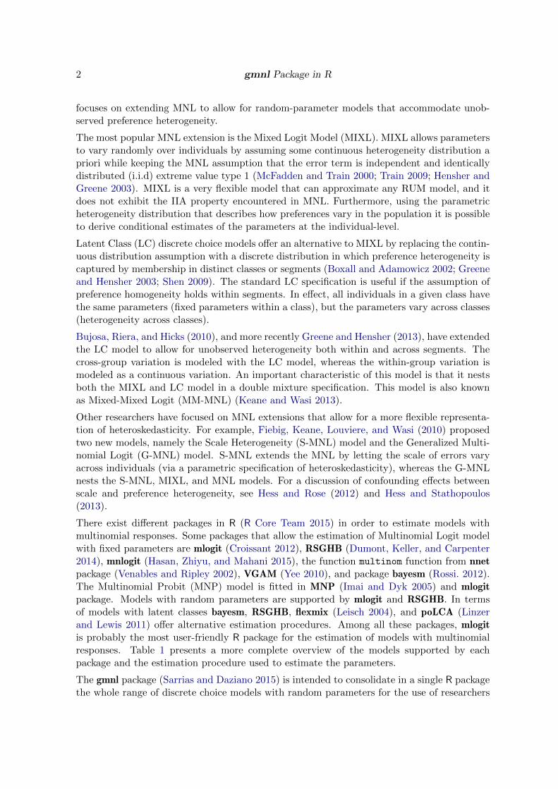
3.7. Estimating LC and MM-MNL models

The next example shows how an LC model with two classes can be estimated:

Elec.lc <- gmnl(choice ~ pf + cl + loc + wk + tod + seas| 0 |

0 | 0 | 1,

data = Electr,

subset = 1:3000,

model = 'lc',panel = TRUE,

Q = 2)

## Estimating LC model

Note that for the LC model, one needs to specify at least a constant in the fifth part of theformula. If the class assignment wiq is also determined by socio-economic characteristics,those covariates can also be included in the fifth part. The LC model is estimated by typingmodel = "lc", and the prespecified number of classes is indicated with the argument Q.

summary(Elec.lc)

##



##

## Call:

## gmnl(formula = choice ~ pf + cl + loc + wk + tod + seas | 0 |

## 0 | 0 | 1, data = Electr, subset = 1:3000, model = "lc",

## Q = 2, panel = TRUE, method = "bfgs")

##


##

## 1 2 3 4

## 0.215 0.303 0.217 0.265

##


##

## Coefficients:


## class.1.pf -0.4458 0.0876 -5.09 3.6e-07 ***

## class.1.cl -0.1847 0.0301 -6.14 8.3e-10 ***

## class.1.loc 1.2144 0.1618 7.50 6.2e-14 ***

## class.1.wk 0.9641 0.1429 6.75 1.5e-11 ***

## class.1.tod -3.2184 0.6880 -4.68 2.9e-06 ***

## class.1.seas -3.4865 0.6929 -5.03 4.9e-07 ***

## class.2.pf -0.8431 0.0968 -8.71 < 2e-16 ***

## class.2.cl -0.1242 0.0453 -2.74 0.0061 **

## class.2.loc 1.6445 0.2689 6.12 9.6e-10 ***

## class.2.wk 1.4139 0.2120 6.67 2.6e-11 ***

## class.2.tod -9.3732 0.8676 -10.80 < 2e-16 ***

## class.2.seas -9.2647 0.8847 -10.47 < 2e-16 ***

## (class)2 -0.2200 0.0788 -2.79 0.0052 **

## ---

## Signif. codes: 0 '***' 0.001 '**' 0.01 '*' 0.05 '.' 0.1 ' ' 1

##






Finally, the next example estimates an MM-MNL with two mixtures of normal:

Elec.mm <- gmnl(choice ~ pf + cl + loc + wk + tod + seas| 0 | 0 | 0 | 1,

data = Electr,

subset = 1:3000,

model = 'mm',R = 50,

panel = TRUE,

ranp = c(pf = "n", cl = "n", loc = "n",


wk = "n", tod = "n", seas = "n"),

Q = 2,

iterlim = 500)

## Estimating MM-MNL model

summary(Elec.mm)

##


##

## Call:


## 0 | 0 | 1, data = Electr, subset = 1:3000, model = "mm",

## ranp = c(pf = "n", cl = "n", loc = "n", wk = "n", tod = "n",

## seas = "n"), R = 50, Q = 2, panel = TRUE, iterlim = 500,

## method = "bfgs")

##


##

## 1 2 3 4

## 0.215 0.303 0.217 0.265

##


##

## Coefficients:


## class.1.pf -1.28047 0.12281 -10.43 < 2e-16 ***

## class.1.cl -0.49715 0.08070 -6.16 7.2e-10 ***

## class.1.loc 0.64457 0.24097 2.67 0.00747 **

## class.1.wk 0.71243 0.21824 3.26 0.00110 **

## class.1.tod -11.62539 1.02751 -11.31 < 2e-16 ***

## class.1.seas -12.65728 1.13964 -11.11 < 2e-16 ***

## class.2.pf -0.43574 0.11588 -3.76 0.00017 ***

## class.2.cl 0.08464 0.08288 1.02 0.30714

## class.2.loc 3.38622 0.38187 8.87 < 2e-16 ***

## class.2.wk 2.72092 0.32689 8.32 < 2e-16 ***

## class.2.tod -4.71641 1.05415 -4.47 7.7e-06 ***

## class.2.seas -4.64754 0.96000 -4.84 1.3e-06 ***

## class.1.sd.pf 0.10535 0.03941 2.67 0.00750 **

## class.1.sd.cl 0.26899 0.05833 4.61 4.0e-06 ***

## class.1.sd.loc 0.00759 0.26552 0.03 0.97718

## class.1.sd.wk 0.11417 0.58066 0.20 0.84413

## class.1.sd.tod 2.20521 0.45035 4.90 9.8e-07 ***

## class.1.sd.seas 2.32199 0.45198 5.14 2.8e-07 ***

## class.2.sd.pf 0.19696 0.03372 5.84 5.2e-09 ***


## class.2.sd.cl 0.35530 0.07492 4.74 2.1e-06 ***

## class.2.sd.loc 0.58709 0.28699 2.05 0.04079 *

## class.2.sd.wk 1.10037 0.30323 3.63 0.00028 ***

## class.2.sd.tod 1.40252 0.51868 2.70 0.00685 **

## class.2.sd.seas 0.07311 0.25655 0.28 0.77565

## (class)2 -0.13719 0.07844 -1.75 0.08028 .

## ---

## Signif. codes: 0 '***' 0.001 '**' 0.01 '*' 0.05 '.' 0.1 ' ' 1

##







The specification is similar to that of the LC model, but we now allow the parameters in eachclass to be normally distributed using the argument ranp. It is worth mentioning that thenumber of iterations required for this model is greater than that for previous models. Forthat reason we have set the maximum of iterations at 500 using the argument iterlim.

3.8. Willingness-to-pay space

Willingness-to-pay space models reparameterize the parameter space in such a way that themarginal WTP for each attribute is directly estimated rather than the marginal utility (prefer-ence parameters). Train and Weeks (2005) and Sonnier, Ainslie, and Otter (2007) extend theWTP-space approach by allowing random parameters (and, consequently, random willingness-to-pay measures). The WTP-space approach is very appealing because it allows the analystto estimate the WTP heterogeneity distribution directly (Scarpa, Thiene, and Train 2008).

To illustrate the concept of WTP space, and how it can be estimated using gmnl, we will firstshow the case without random parameters. The standard procedure to derive willingness-to-pay measures is to start with a model in preference space. For example, consider the simpleconditional logit model,

clogit <- gmnl(choice ~ pf + cl + loc + wk + tod + seas| 0,

data = Electr,

subset = 1:3000)

summary(clogit)

##


##

## Call:

## gmnl(formula = choice ~ pf + cl + loc + wk + tod + seas | 0,

## data = Electr, subset = 1:3000, method = "nr")


##


##

## 1 2 3 4

## 0.215 0.303 0.217 0.265

##


##

## Coefficients:


## pf -0.6113 0.0548 -11.15 < 2e-16 ***

## cl -0.1398 0.0204 -6.85 7.2e-12 ***

## loc 1.1986 0.1197 10.01 < 2e-16 ***

## wk 1.0304 0.1063 9.69 < 2e-16 ***

## tod -5.4540 0.4341 -12.56 < 2e-16 ***

## seas -5.6648 0.4419 -12.82 < 2e-16 ***

## ---

## Signif. codes: 0 '***' 0.001 '**' 0.01 '*' 0.05 '.' 0.1 ' ' 1

##

## Optimization of log-likelihood by Newton-Raphson maximisation




## Exit of MLE: gradient close to zero

To estimate the willingness to pay for each attribute, one needs to divide each attributeparameter by that of price pf. This ratio can be easily retrieved using the function wtp.gmnl:

wtp.gmnl(clogit, wrt = "pf")

##

## Willigness-to-pay respect to: pf

##


## cl 0.2287 0.0358 6.38 1.8e-10 ***

## loc -1.9610 0.2304 -8.51 < 2e-16 ***

## wk -1.6858 0.1949 -8.65 < 2e-16 ***

## tod 8.9226 0.2025 44.07 < 2e-16 ***

## seas 9.2675 0.2164 42.83 < 2e-16 ***

## ---

## Signif. codes: 0 '***' 0.001 '**' 0.01 '*' 0.05 '.' 0.1 ' ' 1

The argument wrt = "pf" indicates that all the parameters should be divided by the param-eter of the attribute pf.

Another way to estimate the same WTP coefficients is to use the S-MNL model. We needfirst to compute the negative of the price coefficient using the mlogit.data function:


ElectrO <- mlogit.data(Electricity, id = "id", choice = "choice",

varying = 3:26, shape = "wide", sep = "",

opposite = c("pf"))

Next, we need to set the values for the price parameter and τ at 1 and 0, respectively. Thefixed argument is used to set these values.

start <- c(1, 0, 0, 0, 0, 0, 0, 0)

wtps <- gmnl(choice ~ pf + cl + loc + wk + tod + seas|0 | 0 | 0 | 1,

data = ElectrO,

model = "smnl",

subset = 1:3000,

R = 1,

fixed = c(TRUE, FALSE, FALSE, FALSE, FALSE,

FALSE, TRUE, FALSE),

panel = TRUE,

start = start,

method = "bhhh",

iterlim = 500)


Note also that we fitted the S-MNL model with a constant in the scale. This constant, after aproper transformation, will represent the price parameter. Since we are working with a fixedparameter model, the number of draws is set equal to 1.

summary(wtps)

##


##

## Call:


## 0 | 0 | 1, data = ElectrO, subset = 1:3000, model = "smnl",

## start = start, R = 1, panel = TRUE, fixed = c(TRUE, FALSE,

## FALSE, FALSE, FALSE, FALSE, TRUE, FALSE), method = "bhhh",

## iterlim = 500)

##


##

## 1 2 3 4

## 0.215 0.303 0.217 0.265

##


##

## Coefficients:



## cl -0.2287 0.0361 -6.34 2.4e-10 ***

## loc 1.9610 0.2284 8.59 < 2e-16 ***

## wk 1.6858 0.1915 8.80 < 2e-16 ***

## tod -8.9226 0.2025 -44.06 < 2e-16 ***

## seas -9.2675 0.2166 -42.79 < 2e-16 ***

## het.(Intercept) -0.4922 0.0917 -5.37 7.9e-08 ***

## ---

## Signif. codes: 0 '***' 0.001 '**' 0.01 '*' 0.05 '.' 0.1 ' ' 1

##

## Optimization of log-likelihood by BHHH maximisation




## Exit of MLE: successive function values within tolerance limit


Each value in the output represents the WTP estimates for each respective attribute. Notethat these WTP estimates are the same as those obtained using the wtp.gmnl function. Theprice coefficient can be obtained using the following transformation:

- exp(coef(wtps)["het.(Intercept)"])

## het.(Intercept)

## -0.611

If one requires the standard error for the price coefficient the deltamethod function from themsm (Jackson 2011) package can be used in the following way:

library("msm")

estmean <- coef(wtps)

estvar <- vcov(wtps)

se <- deltamethod(~ - exp(x6), estmean, estvar, ses = TRUE)

se

## [1] 0.056

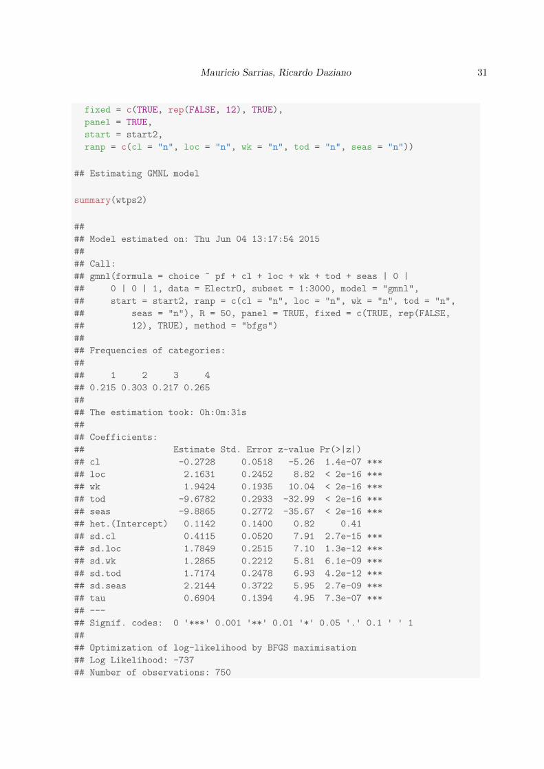
Using the same idea, one can let the WTP to vary across individuals. To do so, we canestimate a G-MNL where the parameter of price and γ are fixed as in the previous example:

start2 <- c(1, coef(wtps), rep(0.1, 5), 0.1, 0)

wtps2 <- gmnl(choice ~ pf + cl + loc + wk + tod + seas|0 | 0 | 0 | 1,

data = ElectrO,

subset = 1:3000,

model = "gmnl",

R = 50,


fixed = c(TRUE, rep(FALSE, 12), TRUE),

panel = TRUE,

start = start2,

ranp = c(cl = "n", loc = "n", wk = "n", tod = "n", seas = "n"))


summary(wtps2)

##


##

## Call:


## 0 | 0 | 1, data = ElectrO, subset = 1:3000, model = "gmnl",

## start = start2, ranp = c(cl = "n", loc = "n", wk = "n", tod = "n",

## seas = "n"), R = 50, panel = TRUE, fixed = c(TRUE, rep(FALSE,

## 12), TRUE), method = "bfgs")

##


##

## 1 2 3 4

## 0.215 0.303 0.217 0.265

##


##

## Coefficients:


## cl -0.2728 0.0518 -5.26 1.4e-07 ***

## loc 2.1631 0.2452 8.82 < 2e-16 ***

## wk 1.9424 0.1935 10.04 < 2e-16 ***

## tod -9.6782 0.2933 -32.99 < 2e-16 ***

## seas -9.8865 0.2772 -35.67 < 2e-16 ***

## het.(Intercept) 0.1142 0.1400 0.82 0.41

## sd.cl 0.4115 0.0520 7.91 2.7e-15 ***

## sd.loc 1.7849 0.2515 7.10 1.3e-12 ***

## sd.wk 1.2865 0.2212 5.81 6.1e-09 ***

## sd.tod 1.7174 0.2478 6.93 4.2e-12 ***

## sd.seas 2.2144 0.3722 5.95 2.7e-09 ***

## tau 0.6904 0.1394 4.95 7.3e-07 ***

## ---

## Signif. codes: 0 '***' 0.001 '**' 0.01 '*' 0.05 '.' 0.1 ' ' 1

##








3.9. Individual parameters

Similarly to the Rchoice package (Sarrias 2015), gmnl also allows the analyst to get theconditional estimates for each individual in the sample (see for example Train 2009; Greene2012). Using Bayes’ theorem we obtain

f(βi|yi,Xi,θ) =f(yi|Xi,βi)g(βi|θ)∫

βif(yi|Xi,βi)g(βi|θ)dβi

,

where f(βi|yi,Xi,θ) is the distribution of the individual parameters βi conditional on theobserved sequence of choices, and g(βi|θ) is the unconditional distribution. The conditionalexpectation of βi is thus given by:

E [βi|yi,Xi,θ] =

∫βi

βif(yi|Xi,βi)g(βi|θ)∫βif(yi|Xi,βi)g(βi|θ)dβi

. (5)

The expectation in Equation 5 gives us the conditional mean of the distribution of the randomparameters, which can also be interpreted as the posterior distribution of the individualparameters. Simulators for this conditional expectation are presented below, for both thecontinuous and discrete cases:

βi = E [βi|yi,Xi,θ] =1R

∑Rr=1 βir

∏t f(yit|xit, βir, θ)

1R

∑Rr=1

∏t f(yit|xit, βir, θ)

βi = E [βi|yi,Xi,θq] =

∑Qq=1 βqwiq

∏t f(yit|xit, βir, θq)∑Q

q=1

∏t f(yit|xit, βq, θq)

In order to construct the confidence interval for βi, we can derive an estimator of the condi-tional variance from the point estimates as follows (Greene 2012, chap. 15):

Vi = E[β2i |yi,Xi,θ

]− E [βi|yi,Xi,θ]2 .

An approximate normal-based 95% confidence interval can be then constructed as βi±1.96×V

1/2i .

The gmnl package uses these formulae to compute the individual parameters along with their95% confidence interval. As an illustration, we can plot the kernel density of the individuals’conditional mean for the loc parameter using Elec.cor model by typing the following:

plot(Elec.cor, par = "loc", effect = "ce", type = "density",

col = "grey")


Figure 1 displays the distribution of the individuals’ conditional mean for the parameter ofloc. The gray area gives us the proportion of individuals with a positive conditional mean.

The 95% confidence interval of the conditional mean for the first 30 individuals is shown inFigure 2, which was plotted using the following syntax:5

plot(Elec.cor, par = "loc", effect = "ce", ind = TRUE, id = 1:30)

Another important function in gmnl is effect.gmnl. This function allows the users to get theindividuals’ conditional mean of both the preference parameters and the willingness-to-paymeasures. For example, one can plot the individual conditional mean and standard errors(Figure 2) by typing:

bi.loc <- effect.gmnl(Elec.cor, par = "loc", effect = "ce")

summary(bi.loc$mean)

## Min. 1st Qu. Median Mean 3rd Qu. Max.

## -0.79 0.42 2.04 2.12 3.46 7.13

summary(bi.loc$sd.est)


## 0.113 0.564 0.795 0.866 1.130 1.860

The conditional mean of the willingness to pay for “loc” (wtp = βi,loc/βpf ) for all individualsin the sample can be obtained using:

wtp.loc <- effect.gmnl(Elec.cor, par = "loc", effect = "wtp", wrt = "pf")

Note that the argument par is the variable whose parameter goes in the numerator, and theargument wrt is a string indicating which parameter goes in the denominator.

summary(wtp.loc$mean)


## -8.19 -3.98 -2.35 -2.44 -0.48 0.91

summary(wtp.loc$sd.est)


## 0.130 0.648 0.914 0.996 1.300 2.130

4. Conclusions

5gmnl uses plotrix package (Lemon 2006) to create the confidence interval graph.


The package gmnl implements the maximum likelihood estimator of random parameter logitmodels with heterogeneity distributions that can be continuous, discrete, or discrete-continuousmixtures. In this paper we have shown how gmnl can fit several extensions to the standardmultinomial logit model, including the recently derived mixed-mixed multinomial logit (MM-MNL). To our knowledge there is no other widely available statistical package that has imple-mented the maximum simulated likelihood estimator of MM-MNL, and we want to highlightthat gmnl makes use of analytical expressions of the gradient. gmnl is also the first imple-mentation in R of the estimator of the scale heterogeneity multinomial logit (S-MNL), thegeneralized multinomial logit (G-MNL), and the latent class logit (LC). Whereas there areother packages in R for the estimation of MIXL, gmnl allows for the inclusion of individual-specific variables to explain the mean of the random parameters for a mixture of deterministictaste variations and unobserved preference heterogeneity. In addition, gmnl also implementsJohnson Sb heterogeneity distributions.

Another key post-estimation functionality of gmnl that we have illustrated in this paper isthe derivation of conditional point and interval estimates of either the random parametersor willingness-to-pay measures at the individual level. Random parameter models can beused to make inference on the preference parameters of each individual in the sample, butmost packages that estimate MIXL models lack a command to produce individual-level esti-mates. gmnl is able to compute individual parameters for all generalized logit models thatare implemented in the package, including G-MNL, MIXL, and LC.

Additional functionalities that we expect to incorporate in the future are the consideration ofdifferent choice sets for each individual and the implementation of different methods for theconstruction of confidence intervals of willingness-to-pay measures.


References

Boxall PC, Adamowicz WL (2002). “Understanding Heterogeneous Preferences in RandomUtility Models: A Latent Class Approach.” Environmental and Resource Economics, 23(4),421–446.

Bujosa A, Riera A, Hicks RL (2010). “Combining Discrete and Continuous Representationsof Preference Heterogeneity: A Latent Class Approach.” Environmental and ResourceEconomics, 47(4), 477–493.

Croissant Y (2012). “Estimation of Multinomial Logit Models in R: The mlogit Packages.”R package version 0.2-2. URL http://cran.r-project.org/web/packages/mlogit/

vignettes/mlogit.pdf.

Dumont J, Keller J, Carpenter C (2014). RSGHB: Functions for Hierarchical BayesianEstimation: A Flexible Approach. R package version 1.0.2, URL http://CRAN.R-project.

org/package=RSGHB.

Fiebig DG, Keane MP, Louviere J, Wasi N (2010). “The Generalized Multinomial LogitModel: Accounting for Scale and Coefficient Heterogeneity.” Marketing Science, 29(3),393–421.

Gourieroux C, Monfort A (1997). Simulation-based Econometric Methods. Oxford UniversityPress.

Greene WH (2012). Econometric Analysis. 7th edition. Prentice Hall.

Greene WH, Hensher DA (2003). “A Latent Class Model for Discrete Choice Analysis: Con-trasts With Mixed Logit.”Transportation Research Part B: Methodological, 37(8), 681–698.

Greene WH, Hensher DA (2010). “Does Scale Heterogeneity Across Individuals Matter? AnEmpirical Assessment of Alternative Logit Models.” Transportation, 37(3), 413–428.

Greene WH, Hensher DA (2013). “Revealing Additional Dimensions of Preference Hetero-geneity in a Latent Class Mixed Multinomial Logit Model.” Applied Economics, 45(14),1897–1902.

Hajivassiliou VA, Ruud PA (1986). “Classical Estimation Methods for LDV Models UsingSimulation.” In RF Engle, D McFadden (eds.), Handbook of Econometrics, volume 4 ofHandbook of Econometrics, chapter 40, pp. 2383–2441. Elsevier.

Hasan A, Zhiyu W, Mahani AS (2015). mnlogit: Multinomial Logit Model. R package version1.2.1, URL http://CRAN.R-project.org/package=mnlogit.

Henningsen A, Toomet O (2011). “maxLik: A Package for Maximum Likelihood Estimationin R.” Computational Statistics, 26(3), 443–458.

Hensher DA, Greene WH (2003). “The Mixed Logit Model: The State of Practice.” Trans-portation, 30(2), 133–176.

http://cran.r-project.org/web/packages/mlogit/vignettes/mlogit.pdf

http://cran.r-project.org/web/packages/mlogit/vignettes/mlogit.pdf

http://CRAN.R-project.org/package=RSGHB

http://CRAN.R-project.org/package=RSGHB

http://CRAN.R-project.org/package=mnlogit


Hess S, Ben-Akiva M, Gopinath D, Walker J (2011). “Advantages of Latent Class OverContinuous Mixture of Logit Models.” Working paper, Institute for Transport Studies,University of Leeds.

Hess S, Rose JM (2012). “Can Scale and Coefficient Heterogeneity be Separated in RandomCoefficients Models?” Transportation, 39(6), 1225–1239.

Hess S, Stathopoulos A (2013). “Linking Response Quality to Survey Engagement: A Com-bined Random Scale and Latent Variable Approach.” Journal of Choice Modelling, 7, 1–12.

Imai K, Dyk DAV (2005). “MNP: R Package for Fitting the Multinomial Probit Model.”Journal of Statistical Software, 14(3), 1–32. URL http://www.jstatsoft.org/v14/i03.

Jackson CH (2011). “Multi-State Models for Panel Data: The msm Package for R.” Journalof Statistical Software, 38(8), 1–29. URL http://www.jstatsoft.org/v38/i08/.

Keane M, Wasi N (2013). “Comparing Alternative Models of Heterogeneity in ConsumerChoice Behavior.” Journal of Applied Econometrics, 28(6), 1018–1045.

Kleiber C, Zeileis A (2008). Applied Econometrics with R. Springer-Verlag, New York. URLhttp://CRAN.R-project.org/package=AER.

Lee LF (1992). “On Efficiency of Methods of Simulated Moments and Maximum SimulatedLikelihood Estimation of Discrete Response Models.” Econometric Theory, 8(04), 518–552.

Leisch F (2004). “FlexMix: A General Framework for Finite Mixture Models and LatentClass Regression in R.” Journal of Statistical Software, 11(8), 1–18. URL http://www.

jstatsoft.org/v11/i08/.

Lemon J (2006). “Plotrix: A Package in the Red Light District of R.” R-News, 6(4), 8–12.

Linzer DA, Lewis JB (2011). “poLCA: An R Package for Polytomous Variable Latent ClassAnalysis.” Journal of Statistical Software, 42(10), 1–29. URL http://www.jstatsoft.

org/v42/i10/.

McFadden D (1974). “Conditional Logit Analysis of Qualitative Choice Behavior.” In P Zarem-bka (ed.), Frontiers in Econometrics, pp. 105–142. Academic Press, New York.

McFadden D, Train K (2000). “Mixed MNL Models for Discrete Response.” Journal of AppliedEconometrics, 15(5), 447–470.

R Core Team (2015). R: A Language and Environment for Statistical Computing. R Founda-tion for Statistical Computing, Vienna, Austria. URL http://www.R-project.org.

Rossi P (2012). bayesm: Bayesian Inference for Marketing/Micro-econometrics. R packageversion 2.2-5, URL http://CRAN.R-project.org/package=bayesm.

Sarrias M (2015). Rchoice: Discrete Choice (Binary, Poisson and Ordered) Models withRandom Parameters. R package version 0.3, URL http://CRAN.R-project.org/package=

Rchoice.

Sarrias M, Daziano R (2015). gmnl: Multinomial Logit Models with Random Parameters. Rpackage version 1.1, URL http://CRAN.R-project.org/package=gmnl.

http://www.jstatsoft.org/v14/i03

http://www.jstatsoft.org/v38/i08/

http://CRAN.R-project.org/package=AER





http://www.R-project.org

http://CRAN.R-project.org/package=bayesm

http://CRAN.R-project.org/package=Rchoice

http://CRAN.R-project.org/package=Rchoice

http://CRAN.R-project.org/package=gmnl


Scarpa R, Thiene M (2005). “Destination Choice Models for Rock Climbing in the Northeast-ern Alps: A Latent-class Approach Based on Intensity of Preferences.” Land Economics,81(3), 426–444.

Scarpa R, Thiene M, Train K (2008). “Utility in Willingness to Pay Space: A Tool to AddressConfounding Random Scale Effects in Destination Choice to the Alps.” American Journalof Agricultural Economics, 90(4), 994–1010.

Shen J (2009). “Latent Class Model or Mixed Logit Model? A Comparison by TransportMode Choice Data.” Applied Economics, 41(22), 2915–2924.

Sonnier G, Ainslie A, Otter T (2007). “Heterogeneity Distributions of Willingness-to-Pay inChoice Models.” Quantitative Marketing and Economics, 5(3), 313–331.

Train K (2009). Discrete Choice Methods with Simulation. 2nd edition. Cambridge UniversityPress.

Train K, Weeks M (2005). “Discrete Choice Models in Preference Space and Willingness-to-Pay Space.” In R Scarpa, A Alberini (eds.), Applications of Simulation Methods inEnvironmental and Resource Economics, volume 6 of The Economics of Non-Market Goodsand Resources, pp. 1–16. Springer Netherlands. ISBN 978-1-4020-3683-5. doi:10.1007/

1-4020-3684-1_1. URL http://dx.doi.org/10.1007/1-4020-3684-1_1.

Train KE (2008). “EM Algorithms for Nonparametric Estimation of Mixing Distributions.”Journal of Choice Modelling, 1(1), 40–69.

Trautmann H, Steuer D, Mersmann O, Bornkamp B (2014). truncnorm: Truncated Nor-mal Distribution. R package version 1.0-7, URL http://CRAN.R-project.org/package=

truncnorm.

Venables WN, Ripley BD (2002). Modern Applied Statistics with S. Fourth edition. Springer-Verlag, New York. ISBN 0-387-95457-0, URL http://www.stats.ox.ac.uk/pub/MASS4.

Yee TW (2010). “The VGAM Package for Categorical Data Analysis.” Journal of StatisticalSoftware, 32(10), 1–34.

Zeileis A, Croissant Y (2010). “Extended Model Formulas in R: Multiple Parts and MultipleResponses.” Journal of Statistical Software, 34(1), 1–13. URL http://www.jstatsoft.

org/v34/i01/.

Zeileis A, Hothorn T (2002). “Diagnostic Checking in Regression Relationships.” R News,2(3), 7–10. URL http://CRAN.R-project.org/doc/Rnews/.

Affiliation:

Mauricio SarriasDepartment of City and Regional PanningCornell University325 W. Sibley Hall, Ithaca, NY 14853, USA

http://dx.doi.org/10.1007/1-4020-3684-1_1

http://dx.doi.org/10.1007/1-4020-3684-1_1

http://dx.doi.org/10.1007/1-4020-3684-1_1

http://CRAN.R-project.org/package=truncnorm

http://CRAN.R-project.org/package=truncnorm

http://www.stats.ox.ac.uk/pub/MASS4



http://CRAN.R-project.org/doc/Rnews/


E-mail: [email protected]: https://msarrias.weebly.com

Ricardo A. DazianoSchool of Civil and Environmental EngineeringCornell University305 Hollister Hall, Ithaca, NY 14850, USAE-mail : [email protected]: http://www.cee.cornell.edu/research/groups/daziano/

mailto:[email protected]

https://msarrias.weebly.com

mailto:[email protected]

http://www.cee.cornell.edu/research/groups/daziano/


−2 0 2 4 6 8

0.00

0.05

0.10

0.15

Conditional Distribution for loc

E(βi^)

Den

sity

Figure 1: Kernel density of the individuals’ conditional mean.


0 5 10 15 20 25 30

−2

02

46

8

95% Probability Intervals for loc

Individuals

E(β

i^)

Figure 2: 95% confident interval for the conditional means.

multinomial logit models with continuous and discrete

Documents