Dynamic Assortment Optimization with a Multinomial

Logit Choice Model and Capacity Constraint

Paat Rusmevichientong∗ Zuo-Jun Max Shen† David B. Shmoys‡

Cornell University UC Berkeley Cornell University

September 22, 2009

Abstract

We consider an assortment optimization problem where a retailer chooses an assortment of

products that maximizes the profit subject to a capacity constraint. The demand is represented

by a multinomial logit choice model. We consider both the static and dynamic optimization

problems. In the static problem, we assume that the parameters of the logit model are known

in advance; we then develop a simple algorithm for computing a profit-maximizing assortment

based on the geometry of lines in the plane, and derive structural properties of the optimal

assortment. For the dynamic problem, the parameters of the logit model are unknown and

must be estimated from data. By exploiting the structural properties found for the static

problem, we develop an adaptive policy that learns the unknown parameters from past data,

and at the same time, optimizes the profit. Numerical experiments based on sales data from an

online retailer indicate that our policy performs well.

1. Introduction

The problem of learning customer preferences and offering a profit-maximizing assortment of prod-

ucts, subject to a capacity constraint, has applications in retail, online advertising, and revenue

management. For instance, given a limited shelf capacity, a retailer must determine the assortment

of products that maximizes the profit (see, for example, Mahajan and van Ryzin, 1998, 2001). The

retailer might not know the demand a priori, and a customer’s product selection often depends

on the assortment offered. In this case, the retailer can learn the demand distribution by offering∗School of Operations Research and Information Engineering, Cornell University, Ithaca, NY 14853, USA. E-mail:

paatrus@cornell.edu†Department of Industrial Engineering and Operations Research, University of California–Berkeley, 4129 Etchev-

erry Hall, Berkeley, CA 94720, USA. E-mail: shen@ieor.berkeley.edu‡School of Operations Research and Information Engineering and Department of Computer Science, Cornell

University, Ithaca, NY 14853, USA. E-mail: shmoys@cs.cornell.edu

1

different assortments, observing purchases, and estimating the demand model from past sales and

assortment decisions (Caro and Gallien, 2007).

In online advertising, the capacity constraint may represent the limited number of locations on

the web page where the ads can appear. The demand for each product corresponds to the number

of customers who click on the ad. The probability that a customer will click on a particular ad will

likely depend on the assortment of ads shown. Given the uncertainty in the demand for each ad and

the limited number of locations where the ads can be shown, we must decide on the assortment of

ads that will generate the most profit, adjusting our assortment decisions, and refining our demand

estimates over time as new data arrive.

Modeling customer choice behavior and estimating demand distributions are active areas of

research in revenue management. When the choice model is known, the focus is to determine the

assortment of itinerary and fare combinations that maximizes the total revenue (see, for example,

Talluri and van Ryzin, 2004; Liu and van Ryzin, 2008; Kunnumkal and Topaloglu, 2008; and Zhang

and Adelman, 2008). When the parameters of the demand distribution are unknown, researchers

have developed techniques for estimating the choice model from sales data (Ratliff et al., 2007;

Vulcano et al., 2008).

1.1 The Model

Motivated by the above applications, we formulate a stylized dynamic assortment optimization

model that captures some of the issues commonly present in these problems, namely the capacity

constraint, the uncertainty in the demand distribution, and the dependence of the purchase or

selection probability on the assortment offered. Assume that we have N products indexed by

1, 2, . . . , N . Let w = (w1, . . . , wN ) ∈ RN+ denote a vector of marginal profits, where for each i,

wi > 0 denotes the marginal profit of product i. The option of no purchase is denoted by 0 with

w0 = 0. Through appropriate scaling, we will assume without loss of generality that wi ≤ 1 for

all i. Due to a capacity constraint, we can offer at most C products to the customers, where C ≥ 2.

The goal is to determine a profit-maximizing assortment of at most C products.

We represent the demand using the multinomial logit (MNL) choice model, which is one of the

most commonly used choice models in economics, marketing, and operations management (see,

Ben-Akiva and Lerman (1985), Anderson et al. (1992), Mahajan and van Ryzin (1998), and the

references therein). Under the MNL model, each customer chooses the product that maximizes her

utility, where the utility Ui of product i is given by: Ui = µi + ζi, where µi ∈ R denotes the mean

utility that the customer assigns to product i. We assume that ζ0, . . . , ζN are independent and

2

identically distributed random variables having a Gumbel distribution with location parameter 0

and scale parameter 1. Without loss of generality, we set µ0 = 0, and let µ = (µ1, . . . , µN ) ∈ RN

denote the vector of mean utilities.

Following the terminology in Vulcano et al. (2008), we define a “customer preference vector”

v = (v1, . . . , vN ) ∈ RN+ , where vi = eµi for all i, and set v0 = 1. Given an assortment S ⊆

{1, 2, . . . , N}, the probability θi(S) that a customer chooses product i is given by:

θi(S) =

vi/(1 +

∑k∈S vk

), if i ∈ S ∪ {0},

0, otherwise ,(1)

and the expected profit f(S) associated with the assortment S is defined by:

f(S) =∑i∈S

wiθi(S) =∑

i∈S wivi

1 +∑

i∈S vi. (2)

We will consider two problems: static and dynamic optimizations. In static optimization, we

assume that v is known in advance, and we wish to find the assortment with at most C products

that gives the maximum expected profit, corresponding to the following combinatorial optimization

problem:

(Capacitated MNL) Z∗ = max {f(S) : S ⊆ {1, . . . , N} and |S| ≤ C} . (3)

In dynamic optimization, on the other hand, the vector v is unknown, and we have to infer its value

by offering different assortments over time and observing the customer selections. For simplicity,

we will assume that we can offer an assortment to a single customer in each time period1. For

each assortment S ⊆ {1, . . . , N} and t ≥ 1, let the random variables Xt(S) and Yt(S) denote the

selection and the reward, respectively, associated with offering the assortment S in period t. The

random variable Xt(S) takes values in {0} ∪ S and has the following probability distribution: for

each i ∈ {0} ∪ S,

Pr {Xt(S) = i} = θi(S) =vi

1 +∑

k∈S vk.

In addition, the random variable Yt(S) is given by Yt(S) = wXt(S), and we have that E [Yt(S)] =∑i∈S wi Pr {Xt(S) = i} = f(S). For each t, let Ht denote the set of possible histories until

the end of period t. A policy ψ = (ψ1, ψ2, . . .) is a sequence of functions, where ψt : Ht−1 →

{S ⊆ {1, . . . , N} : |S| ≤ C} selects an assortment of size C or less in period t based on the history

until the end of period t− 1. The T -period cumulative regret under the policy ψ is defined by:

Regret(T, ψ) =T∑t=1

E [Z∗ − Yt(St)] =T∑t=1

E [Z∗ − f(St)] ,

1This assumption is introduced primarily to simplify our exposition. Our analysis extends to the setting where a

single assortment is offered to multiple customers in each period.

3

where S1, S2, . . . , denote the sequence of assortments offered under the policy ψ. Note that St is

a random variable that depends on the selections X1(S1), X2(S2), . . . , Xt−1(St−1) of customers in

the preceding t− 1 periods. We are interested in finding a policy that minimizes the regret, which

is equivalent to maximizing the total expected reward∑T

t=1 E [f(St)] .

1.2 Contributions and Organization

Our work illuminates the structure of the capacitated assortment optimization problem under the

MNL model, both in static and dynamic settings. For static optimization, Example 2.1 shows

how the optimal assortment, under a capacity constraint, exhibits different structural properties

from the optimal solution in the uncapacitated setting. This example demonstrates that we must

be careful in applying our intuition from the uncapacitated problem. Megiddo (1979) presents

a recursive algorithm for optimizing a rational objective function, which can be applied to the

Capacitated MNL problem. Because the algorithm recursively invokes subroutines and traverses

a computational tree, we do not know how changes in the customer preference vector v affect the

optimal assortment and profit. The lack of a transparent relationship between v and Z∗ makes it

very difficult to apply and analyze this algorithm in a dynamic setting, where v is unknown and

must be estimated from data.

So, in Section 2.1, we describe an alternative algorithm – which we refer to as StaticMNL –

that is non-recursive and is based on a simple geometry of lines in the two-dimensional plane.

Although the StaticMNL algorithm builds upon the ideas introduced in Megiddo (1979), our

algorithm demonstrates a simple and transparent relationship between the preference vector v and

the optimal assortment, enabling us to extend it to the dynamic optimization setting. To our

knowledge, this is the first result that characterizes the sensitivity of the optimal assortment to

changes in the customer preferences (see Theorem 2.4).

The StaticMNL algorithm generates a sequence A = 〈A0, A1, . . . , AK〉 of assortments, with

K = O(N2), that is guaranteed to contain the optimal solution (Theorem 2.2). By exploiting the

properties of the MNL model, we show in Theorem 2.5 that the number of distinct assortments in the

sequenceA is of order O(NC). We also prove that the sequence of profits 〈f(A0), f(A1), . . . , f(AK)〉

is unimodal, and establish a lower bound on the difference between the profit of any two consecutive

assortments in the sequence A (Theorem 2.6). We then show how we can exploit these structural

properties to derive an efficient search algorithm based on golden ratio search (Lemma 2.7). To

our knowledge, these structural properties associated with the MNL model are new, and they can

potentially be extended to more complex choice models such as the nested logit (see, for example,

Rusmevichientong et al., 2009).

4

We exploit the geometric insights and the wealth of structural properties to extend the Stat-

icMNL algorithm to the dynamic optimization setting, where v is unknown. In Section 3, we de-

scribe a policy that adaptively learns the customer preference over time, and establish an O(log2 T )

upper bound on the regret. Saure and Zeevi (2008) has improved the regret bound to O (log T )

and prove that this is the minimal possible regret. Our analysis of the regret also establishes a

connection between our estimates of the customer preference and maximum likelihood estimation,

enabling us to generalize our results to the linear-in-parameters utility model. The results of the

numerical experiments in Section 4 based on sales data from an online retailer show that our policy

performs well.

Although our results build upon the existing work in the literature, our refinements enable

us to discover previously unknown relationships between the customer preference and the optimal

assortment in a capacitated setting. The newly discovered insights help us to develop a policy

for joint parameter estimation and assortment optimization. The synthesis of results from diverse

communities to address an important practical problem represents one of the main contributions

of our work.

1.3 Literature Review

This paper contributes to the literature in both static and dynamic assortment planning. The static

assortment planning (where the underlying demand distribution is assumed be known in advance)

has an extensive literature, and we refer the reader to Kok et al. (2008) for an excellent review of

the current state of the art. We will focus on a few papers that are closely related to our work.

Our work is part of a growing literature on modeling customer choice behavior in revenue

management. Talluri and van Ryzin (2004) consider the multi-period single-resource revenue man-

agement problem under a general discrete choice model, where the objective is to determine the

assortment of fare products over time that maximizes the total revenue. They characterize the

optimal assortments in terms of nondominated sets. This pioneering work has been extended to

the general network revenue management setting (see, for example, Shen and Su, 2007; Kunnumkal

and Topaloglu, 2008; Zhang and Adelman, 2008, and the references therein).

The Capacitated MNL model can be viewed as a single-period problem, and is an extension

of the unconstrained optimization problem studied by Gallego et al. (2004) and Liu and van Ryzin

(2008), who describe a beautiful algorithm for finding the optimal assortment based on sorting the

products in a descending order of marginal profits. They use this subroutine as part of the column-

generation method for solving the choice-based linear programming model for network revenue

5

management. As shown in Example 2.1, when there is a capacity constraint, sorting the products

based on marginal profits alone can lead to suboptimal solutions. It turns out that the assortments

generated by the StaticMNL algorithm are similar to the nondominated sets introduced by Talluri

and van Ryzin (2004) (more on this in Section 2.1).

Our dynamic optimization formulation can be viewed as an instance of the multiarmed bandit

problem (see, Lai and Robbins, 1985 and Auer et al., 2002). We can view each product as an

arm whose reward profile is unknown. In each period, we can choose up to C arms (equivalent to

offering up to C products) with the goal of minimizing regret. Many researchers have studied this

problem (see, for example, Anantharam et al., 1987a,b), but most of the literature assumes that

the reward of each arm is independent of the assortment of arms chosen, which is not applicable to

our setting where there are substitution effects.

To our knowledge, the first paper that consider the dynamic optimization where the reward is

contingent on the assortment of arms chosen is the pioneering work of Caro and Gallien (2007), who

consider a stylized multiarmed bandit model assuming independent demand at first, and develop

an effective dynamic index policy for determining the product assortment. They then extend their

model to account for substitution among products, but their substitution model is very different

from the MNL model considered here.

Although this is not our focus, our work in dynamic optimization is also related to the research

on estimating the customer choice behavior from data. Much of the research in this area focuses

on developing techniques for inferring the underlying demand from censored observations. Ratliff

et al. (2007) describe a heuristic for unconstraining the demand across multiple flights and fare

classes. Vulcano et al. (2008) consider an approach for estimating substitutes and lost sales based

on first-choice demand. In our formulation, we ignore the inventory consideration and assume that

every product in the assortment is available to the customers. We focus primarily on designing an

adaptive assortment policy with minimal regret.

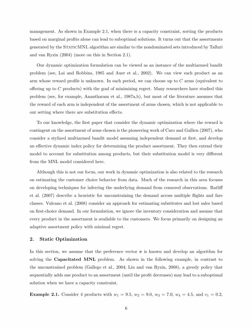
2. Static Optimization

In this section, we assume that the preference vector v is known and develop an algorithm for

solving the Capacitated MNL problem. As shown in the following example, in contrast to

the unconstrained problem (Gallego et al., 2004; Liu and van Ryzin, 2008), a greedy policy that

sequentially adds one product to an assortment (until the profit decreases) may lead to a suboptimal

solution when we have a capacity constraint.

Example 2.1. Consider 4 products with w1 = 9.5, w2 = 9.0, w3 = 7.0, w4 = 4.5, and v1 = 0.2,

6

v2 = 0.6, v3 = 0.3, v4 = 5.2. The expected profit for each assortment is given in the table below,

and the maximum of each column is highlighted in bold.

S f(S) S f(S) S f(S) S f(S)

{1} 1.583 {1, 2} 4.056 {1, 2, 3} 4.476 {1, 2, 3, 4} 4.493

{2} 3.375 {1, 3} 2.667 {1, 2, 4} 4.386

{3} 1.615 {1, 4} 3.953 {1, 3, 4} 4.090

{4} 3.774 {2, 3} 3.947 {2, 3, 4} 4.352

{2, 4} 4.253

{3, 4} 3.923

The optimal assortment for each value of C is given by:

C 1 2 3 4

Optimal Assortment {4} {2, 4} {1, 2, 3} {1, 2, 3, 4}

When C = 1 and C = 2, the optimal assortments include product 4, which has the lowest marginal

profit, but this product is not included in the optimal assortment when C = 3. Yet, it re-appears

when there is no capacity constraint (C = 4). Moreover, for C = 3, under the greedy policy that

sequentially adds a product until the profit decreases, we would get the assortment {1, 2, 4}, which

is suboptimal.

Although we can apply the algorithm of Megiddo (1979) to solve the Capacitated MNL

problem, the algorithm is recursive and difficult to visualize. Moreover, the algorithm does not

provide a simple and transparent relationship between the preference vector v and the optimal

assortment, making it difficult to analyze its performance in a dynamic setting. In the next section,

we present a geometric algorithm that can be easily visualized (see Example 2.3), and the simple

geometry associated with our method illuminates how the optimal assortment changes with the

parameter v, providing the first sensitivity analysis for this class of problems (Theorem 2.4). We

also derive novel structural properties (Theorems 2.5 and 2.6), which can be used to develop an

efficient search procedure for the optimal assortment (Theorem 2.7).

2.1 A Geometric Non-Recursive Polynomial-time Algorithm

The key idea underlying our algorithm is the observation that we can express the optimal profit

Z∗ in Equation (3) as follows:

Z∗ = max {λ ∈ R : ∃X ⊆ {1, . . . , N}, |X| ≤ C, and f(X) ≥ λ}

= max

{λ ∈ R : ∃X ⊆ {1, . . . , N}, |X| ≤ C, and

∑i∈X

vi (wi − λ) ≥ λ

}

= max

{λ ∈ R : max

X:|X|≤C

∑i∈X

vi (wi − λ) ≥ λ

},

7

where the second equality follows from the definition of the profit function f(·) given in Equation (2).

Let the functions A : R → {X ⊆ {1, . . . , N} : |X| ≤ C} and g : R → R be defined by: for each

λ ∈ R,

A(λ) = arg maxX:|X|≤C

∑i∈X

vi (wi − λ) and g(λ) =∑i∈A(λ)

vi (wi − λ) , (4)

where we break ties arbitrarily. Therefore, Z∗ = max {f (A(λ)) : λ ∈ R}, and to find the optimal

assortment, it suffices to enumerate A(λ) for all values of λ ∈ R. We will show that the collection of

assortments {A(λ) : λ ∈ R} has at most O(N2) sets. For each λ ∈ R, it follows from Proposition 1

in Talluri and van Ryzin (2004) that A(λ) can be interpreted as a nondominated set among all

subsets of size C or less2.

Before we describe the algorithm, let us provide some geometric intuition. For i = 0, 1, . . . , N ,

let the linear function hi : R→ R be defined by: for each λ ∈ R,

h0(λ) = 0 and hi(λ) = vi (wi − λ) , for i = 1, . . . , N. (5)

The number of intersection points among the N+1 lines h0(·), . . . , hN (·) is at most(N+1

2

)= O(N2).

Suppose we sort these intersection points based on their x-coordinates. It follows from Equation (4)

that, for each λ ∈ R, A(λ) corresponds to the top C lines among h0(·), h1(·), . . . , hN (·) whose values

at λ are nonnegative. Then, for an arbitrary λ strictly between two consecutive intersection points,

the ordering of the values hj(λ) = vj (wj − λ) remain constant and their values do not change sign.

Therefore, for any λ strictly between the two consecutive intersection points, A(λ) remains the

same. So, to enumerate A(λ) for all λ ∈ R, it suffices to enumerate all of the intersection points

among the N + 1 lines. This observation forms the basis of the StaticMNL algorithm described

below.

For all 0 ≤ i < j ≤ N with vi 6= vj , let I(i, j) denote the x-coordinate of the intersection point

between the lines hi(·) and hj(·), that is,

hi (I(i, j)) = hj (I (i, j)) ⇔ I(i, j) =viwi − vjwjvi − vj

.

Let τ = ((i1, j1) , . . . , (iK , jK)) denote the ordering of the intersection points, that is, i` < j` for

each ` = 1, . . . ,K and

−∞ ≡ I(i0, j0) < I(i1, j1) ≤ I(i2, j2) ≤ · · · ≤ I(iK , jK) < I(iK+1, jK+1) ≡ +∞, (6)2To apply Proposition 1 in Talluri and van Ryzin (2004), for any assortment S of size C or less, we can define

R(S) =P

i∈S viwi and Q(S) =P

i∈S vi .

8

where we have added the two end points I(i0, j0) and I(iK+1, jK+1) to facilitate our exposition.

Also, let σ0 =(σ0

1, . . . , σ0N

)denote the ordering of the customer preference weights from highest to

lowest, that is,

vσ01≥ · · · ≥ vσ0

N. (7)

The ordering σ0 is the ordering of the lines h1(·), h2(·), . . . , hN (·) at λ = −∞ from the highest to

the lowest values. The StaticMNL algorithm maintains the following four pieces of information

associated with the interval(I (i`, j`) , I (i`+1, j`+1)

):

1. The ordering σ` =(σ`1, . . . , σ

`N

)of the lines h1(·), . . . , hN (·) from the highest to the smallest

values, that is, for all λ ∈(I (i`, j`) , I (it+1, jt+1)

),

hσ`1(λ) ≥ hσ`

2(λ) ≥ · · · ≥ hσ`

N(λ) .

2. The set G` corresponding to the first C elements according to the ordering σ`, that is

G` ={σ`1, . . . , σ

`C

}.

3. The set B` of lines whose values have become negative, that is,

B` ={i : hi(λ) < 0 for λ ∈

(I (i`, j`) , I (it+1, jt+1)

)}.

Since the lines h1(·), . . . , hN (·) are strictly decreasing, B` ⊆ B`+1 for all `.

4. The assortment A` = G` \B`.

The formal description of the StaticMNL policy is given as follows.

StaticMNL

Inputs: The number of intersection points K, the ordering τ = ((i1, j1) , . . . , (iK , jK)) of the

intersection points, and the ordering σ0 of the preference vector v. Let A0 = G0 ={σ0

1, . . . , σ0C

}and B0 = ∅.

Description: For ` = 1, 2, . . . ,K,

• If i` 6= 0, let the permutation σ` be obtained from σ`−1 by transposing i` and j` and set

B` = B`−1.

• If i` = 0, let σ` = σ`−1 and B` = B`−1 ∪ {j`}.• Let G` =

{σ`1, . . . σ

`C

}and A` = G` \B`.

Output: The sequence of assortments A =⟨A` : ` = 0, 1, . . . ,K

⟩.

9

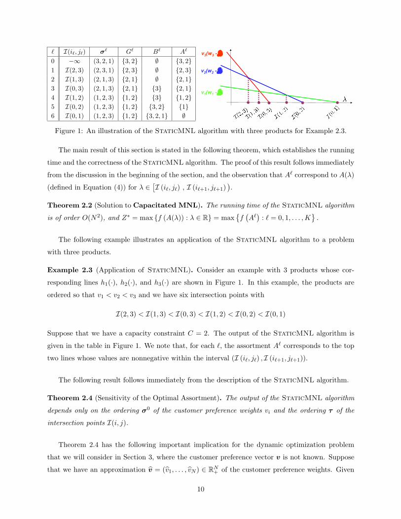
` I(i`, j`) σ` G` B` A`

0 −∞ (3, 2, 1) {3, 2} ∅ {3, 2}1 I(2, 3) (2, 3, 1) {2, 3} ∅ {2, 3}2 I(1, 3) (2, 1, 3) {2, 1} ∅ {2, 1}3 I(0, 3) (2, 1, 3) {2, 1} {3} {2, 1}4 I(1, 2) (1, 2, 3) {1, 2} {3} {1, 2}5 I(0, 2) (1, 2, 3) {1, 2} {3, 2} {1}6 I(0, 1) (1, 2, 3) {1, 2} {3, 2, 1} ∅

v3(w3 - λ)

v2(w2 - λ)

v1(w1 - λ)

Figure 1: An illustration of the StaticMNL algorithm with three products for Example 2.3.

The main result of this section is stated in the following theorem, which establishes the running

time and the correctness of the StaticMNL algorithm. The proof of this result follows immediately

from the discussion in the beginning of the section, and the observation that A` correspond to A(λ)

(defined in Equation (4)) for λ ∈[I (i`, j`) , I (i`+1, j`+1)

).

Theorem 2.2 (Solution to Capacitated MNL). The running time of the StaticMNL algorithm

is of order O(N2), and Z∗ = max {f (A(λ)) : λ ∈ R} = max{f(A`)

: ` = 0, 1, . . . ,K}.

The following example illustrates an application of the StaticMNL algorithm to a problem

with three products.

Example 2.3 (Application of StaticMNL). Consider an example with 3 products whose cor-

responding lines h1(·), h2(·), and h3(·) are shown in Figure 1. In this example, the products are

ordered so that v1 < v2 < v3 and we have six intersection points with

I(2, 3) < I(1, 3) < I(0, 3) < I(1, 2) < I(0, 2) < I(0, 1)

Suppose that we have a capacity constraint C = 2. The output of the StaticMNL algorithm is

given in the table in Figure 1. We note that, for each `, the assortment A` corresponds to the top

two lines whose values are nonnegative within the interval (I (i`, j`) , I (i`+1, j`+1)).

The following result follows immediately from the description of the StaticMNL algorithm.

Theorem 2.4 (Sensitivity of the Optimal Assortment). The output of the StaticMNL algorithm

depends only on the ordering σ0 of the customer preference weights vi and the ordering τ of the

intersection points I(i, j).

Theorem 2.4 has the following important implication for the dynamic optimization problem

that we will consider in Section 3, where the customer preference vector v is not known. Suppose

that we have an approximation v = (v1, . . . , vN ) ∈ RN+ of the customer preference weights. Given

10

v, we can estimate the intersection points I (ik, jk). We can then use the ordering of v and the

ordering of the estimated intersection points as inputs to the StaticMNL algorithm. The above

theorem tells us that as long as the estimated orderings coincide with the true orderings, then the

output of the StaticMNL will be exactly the same as if we know the true value of v.

2.2 Properties of A

In the next two sections, we exploit the geometry associated with the MNL model to derive struc-

tural properties of the sequence of assortmentsA =⟨A0, A1, . . . , AK

⟩generated by the StaticMNL

algorithm. Before we proceed, let us introduce the following assumption that will be used through-

out the rest of the paper. We emphasize that Assumption 2.1 is introduced primarily to simplify

our exposition and to facilitate the discussion of the key ideas without having to worry about

degenerate cases.

Assumption 2.1 (Distinct Customer Preferences and Intersection Points).

(a) The products are indexed so that 0 < v1 < v2 < · · · < vN .

(b) The intersection points are distinct, that is, for any (i, j) 6= (s, t), I(i, j) 6= I(s, t).

Assumption 2.1(a) requires the values of vi to be distinct, while Assumption 2.1(b) requires that

the marginal profit wi are distinct, and no three lines among h1(·), . . . , hN (·) can intersect at the

same point. As a consequence of Assumption 2.1, we observe that every pair of lines hi(·) and

hj(·) will intersect each other, and thus, the number of intersection points K is exactly(N+1

2

). In

addition, we also have a strict ordering of the intersection points, that is,

−∞ ≡ I(i0, j0) < I(i1, j1) < I(i2, j2) < · · · < I(iK , jK) < I(iK+1, jK+1) ≡ +∞ .

The main result of this section is stated in the following theorem. The proof of this result is given

in Appendix A.

Theorem 2.5 (Properties of A). Under Assumption 2.1,

(a) For each ` = 1, . . . ,K, if A` 6= A`−1, then

A` =

(A`−1 \ {j`}

)∪ {i`}, if

∣∣A`∣∣ = C ,(A`−1 \ {j`}

), if

∣∣A`∣∣ < C ,

(b) For any s < C, there is exactly one distinct assortment of size s in the sequence A.

(c) There are at most C(N − C + 1) distinct non-empty assortments in the sequence A.

11

Let us briefly describe the intuition behind the proof the above result. Since the slope of the

lines hi(·) are negative, we can establish a partial ordering among the intersection points of any

three lines (Lemma A.1). This relationship enables us to show that the ordering σ` is obtained

from σ`−1 by a transposition of two adjacent products (to be defined precisely in Lemma A.2).

These two results then allow us to establish Theorem 2.5.

The above theorem shows that each assortment in the sequence A is obtained by either inter-

changing a pair of products or removing a product. Moreover, if the capacity C is fixed, finding

the optimal assortment requires us to search only through O(N) assortments, which is on the same

order as the uncapacitated optimization problem (see Gallego et al., 2004; Liu and van Ryzin,

2008). Given the result of Theorem 2.5, throughout the rest of the paper, we will assume that the

assortments in the sequence A are distinct.

2.3 Unimodality of A and Application to Sampling-based Golden Ratio Search

In this section, we will show that the sequence of profits⟨f(Ai) : i = 0, 1, . . . ,K

⟩is unimodal. To

facilitate our discussion, let β ∈ (0, 1) be defined by

β =min

{mini vi , mini 6=j |vi − vj | , min(i,j)6=(s,t) |I(i, j)− I(s, t)|

}(1 + C maxi vi)

. (8)

For any assortment S of size C or less and {i, j} ⊆ S, we have that

|θi(S)− θj(S)| = |vi − vj |1 +

∑k∈S vk

≥ β ,

and thus, the parameter β is a lower bound on the difference between the selection probabilities of

any two products. Under Assumption 2.1, the parameter β is always positive.

Theorem 2.6 (Unimodality of the Profit Function Over A). Under Assumptions 2.1, if the as-

sortments in the sequence A are distinct, then there exists q ∈ {0, 1, . . . ,K} such that

f(A0)< f

(A1)< · · · < f

(Aq−2

)< f

(Aq−1

)≤ f(Aq) and f (Aq) > f

(Aq+1

)> · · · > f

(AK),

and for each ` /∈ {q, q + 1},∣∣f(A`)− f(A`−1)

∣∣ ≥ β2 .

Proof. Consider an arbitrary `. There are two cases to consider:∣∣A`∣∣ = C and

∣∣A`∣∣ < C. Suppose

that∣∣A`∣∣ = C. It follows from Theorem 2.5(a) that A` =

(A`−1 \ {j`}

)∪{i`} with 1 ≤ i` < j`. Let

12

X = A`−1 \ {i`, j`}. Then, we have

f(A`)− f

(A`−1

)=

∑k∈X wkvk + wi`vi`

1 +∑

k∈X vk + vi`−∑

k∈X wkvk + wj`vj`1 +

∑k∈X vk + vj`

=

(1 +

∑k∈X vk

)(wi`vi` − wj`vj`)−

(∑k∈X wkvk

)(vi` − vj`) + (wi` − wj`) vi`vj`(

1 +∑

k∈X vk + vi`) (

1 +∑

k∈X vk + vj`)

=(vj` − vi`) ·

{−(1 +

∑k∈X vk

) (wi`vi`−wj`

vj`)vi`−vj`

+∑

k∈X wkvk −(wi`

−wj`)vi`vj`

vi`−vj`

}(1 +

∑k∈X vk + vi`

) (1 +

∑k∈X vk + vj`

)=

(vj` − vi`) ·{−(1 +

∑k∈X vk

)I (i`, j`) +

(∑k∈X wkvk

)+ hi` (I (i`, j`))

}(1 +

∑k∈X vk + vi`

) (1 +

∑k∈X vk + vj`

) ,

where the last equality follows from the fact that

I (i`, j`) =wi`vi` − wj`vj`

vi` − vj`and hi` (I (i`, j`)) =

− (wi` − wj`) vi`vj`vi` − vj`

.

Since hi` (I (i`, j`)) = vi` (wi` − I (i`, j`)) and A` = X ∪ {i`}, we have that

f(A`)− f

(A`−1

)=

(vj` − vi`) ·{−I(i`, j`) +

∑k∈A` vk (wk − I (i`, j`))

}(1 +

∑k∈X vk + vi`

) (1 +

∑k∈X vk + vj`

)=

(vj` − vi`) · {g (I(i`, j`))− I(i`, j`)}(1 +

∑k∈X vk + vi`

) (1 +

∑k∈X vk + vj`

) ,where the last equality follows from the definition of g(·) defined in Equation (4), which shows that

g(λ) =∑

k∈A` vk(wk − λ) for I(i`, j`) ≤ λ < I(i`+1, j`+1). In the case where∣∣A`∣∣ < C, we have

that A` = A`−1 \ {j`} by Theorem 2.5(a). Using the same argument as above, we can show that

f(A`)− f

(A`−1

)=

vj` · {g (I(i`, j`))− I(i`, j`)}(1 +

∑`∈X v`

) (1 +

∑`∈X v` + vj`

) .In both cases, the denominator in the expression f

(A`)− f

(A`−1

)is always positive. Also,

since i` < j`, it follows from Assumption 2.1 that vj` − vi` is always positive. From the definition,

g(·) is a continuous, piecewise linear, non-increasing, convex function, and g(Z∗) = Z∗. Thus,

g(λ) − λ > 0 for all λ < Z∗ and g(λ) − λ > 0 for all λ > Z∗. Let q ∈ {0, 1, . . . ,K} denote the

largest index such that I (iq, jq) ≤ Z∗. It follows from Assumption 2.1(b) that

I (i1, j1) < · · · < I (iq−1, jq−1) < I (iq, jq) ≤ Z∗ < I (iq+1, jq+1) < · · · < I (iK , jK) .

Then, it follows that f(A0)< f

(A1)< · · · < f

(Aq−1

)≤ f(Aq) and f (Aq) > f

(Aq+1

)> · · · >

f(AK), which is the desired result.

The function g(λ) − λ is a piecewise linear, strictly decreasing, and convex function which

is zero at Z∗, and the absolute value of its subgradient is bounded below by one. Thus, it

13

is easy to verify that for all λ ∈ R, |g(λ)− λ| ≥ |λ− Z∗| . Thus, if ` /∈ {q, q + 1}, we have

that |g (I(i`, j`))− I(i`, j`)| ≥ min(k,m)6=(s,t) |I(k,m)− I(s, t)|. Therefore, using the expression for

f(A`)− f(A`−1), we conclude that∣∣f (A`)− f (A`−1

)∣∣ ≥ β2, which completes the proof.

Given the sequence of assortments A, if we can evaluate the profit function f(·), it follows from

Theorem 2.6 that we can apply the standard Golden Ratio Search (see, for example, Press et al.,

1999) to find the optimal assortment in O (log(NC)) iterations. It turns out that the unimodality

structure of the sequence of profits can also be exploited to yield an efficient search algorithm in

the dynamic optimization problem, where the preference vector v is unknown. In this case, for

each assortment A` in the sequence A, we can offer it to a sample of customers and compute the

average profit from the resulting sales. We know from Theorem 2.6 that there is a gap of β2 in

the difference between the expected profit of two consecutive assortments. This suggests that, if

the number of customers is sufficiently large, we can use the average profit as a proxy for f(A`),

and apply the standard golden ratio search procedure. This idea is the basis of the sampling-based

golden ratio search described below.

Sampling-Based Golden Ratio Search (Sampling GRS)

Input: A sequence A of assortments and a time horizon T .

Algorithm Description: We perform the standard Golden Ratio search. Whenever we need to

compare the values of two assortments A`1 and A`2 in the sequence A, we check to see if each

assortment has been offered to at least⌈2(log T )/β4

⌉independent customers. If not, then offer

each of these assortments to the customers until we have at least⌈2(log T )/β4

⌉observations for

each assortment. If we have enough data, compare the two assortments based on the average

profits obtained and proceed as in the classical Golden Ratio Search algorithm. At the end of the

Golden Ratio Search, we are left with a single assortment, offer that assortment until the end of

the horizon3.

The idea of using the sample average as an approximation of the true expectation has been

applied in many applications (see, for example, Shapiro, 2003; Swamy and Shmoys, 2005; Levi

et al., 2007). We present the algorithm and its analysis primarily for the sake of completeness.

We will use this algorithm in the next section when we present an adaptive policy for generating

a sequence of assortments. The following lemma establishes a performance bound associated with

our sampling-based golden ratio search; the proof appears in Appendix B.3Instead of waiting until we are left with a single assortment, we can terminate the search procedure when we are

left with a few assortments, say four or five. Then, we can apply the standard multiarmed bandit algorithm (Lai and

Robbins, 1985; Auer et al., 2002). The analysis is essentially the same.

14

Lemma 2.7 (Regret for Sampling-based GRS). Suppose that the sequence A is given, but the

customer preference vector v is unknown. Then, there exists a positive constant a1 that depends

only on C, v, and w such that, for any T ≥ 1, the regret under the Sampling-based Golden

Ratio Search is bounded above by

Regret (T,Sampling GRS) ≤ a1(logN) log T .

We note that by exploiting the unimodality of the sequence of profits and the gap between the

expected profit of any two consecutive assortments, we obtain a regret bound that scales with logN ,

instead of N under the traditional bandit algorithms that tries every assortment in the sequence A.

The Sampling-based GRS algorithm, however, requires a prior knowledge of the gap β. Since

we have an explicit formula for β in Equation (8), we can potentially estimate its value from our

estimates of v (more on this in the next section).

3. Dynamic Optimization

In this section, we address the dynamic optimization problem, where the preference vector v ∈ RN+ is

unknown and must be estimated from past sales and assortment decisions. It follows from Theorem

2.4 that the ordering of v and the ordering of the intersection points among the lines h0(·), . . . , hN (·)

completely determine the outputs of the StaticMNL algorithm. So, instead of estimating the

actual values of v, it suffices to estimate the orderings. There is a simple relationship between

the selection probabilities and the orderings of the intersection points and the customer preference

weights. It follows from the definition of the intersection point I(i, j) that for any assortment S

containing both i and j,

I(i, j) =wivi − wjvjvi − vj

=wiθi (S)− wjθj (S)θi (S)− θj (S)

, (9)

and vi ≤ vj if and only if θi (S) ≤ θj (S).

We can estimate the selection probabilities by counting the number of customers who select a

particular product from an assortment. This idea forms the basis of our proposed policy for the

dynamic optimization. To facilitate our exposition, let E denote the collection of subsets of size C

that “cover” all pairs of products, that is, for all i and j, there exists an assortment S ∈ E with

|S| = C and {i, j} ⊆ S. It is easy to verify that |E| ≤ 5(N/C)2. Here is an example of E .

Example 3.1. Suppose that N = 6 and C = 3. We can define E as follows:

E = {{1, 2, 3}, {4, 5, 6}, {1, 2, 4}, {1, 2, 5}, {1, 2, 6}, {1, 3, 4}, {3, 5, 6}} .

It can be observed that, for all i and j, there exists S ∈ E such that {i, j} ⊆ S.

15

Our policy, which we refer to as Adaptive Assortment (AA), operates in cycles. Each cycle

m ≥ 1 consists of an exploration phase, followed by an exploitation phase. In the exploration phase

of cycle m, we offer each assortment S ∈ E to a single customer and observe her selection. At

the end of the exploration phase, for each assortment S ∈ E and i ∈ S, we estimate the selection

probability Θi(m,S) based on the fraction of customers who selected product i during the past m

cycles. We can then estimate of the ordering of v based on the ordering of Θi(m,S). Also, for

any {i, j} ⊆ S, we can estimate the intersection point between the lines hi(·) and hj(·) based on

Θi(m,S) and Θj(m,S). This gives us an estimated ordering of the intersection points. Using these

estimated orderings as inputs to the StaticMNL algorithm, we obtain as an output a sequence

of assortments A(m). We will show that, with a high probability, the sequence A(m) coincides

with the sequence of assortments A that we would have obtained had we known v a priori. Since

the sequence of assortments A is unimodal under the profit function f(·) by Theorem 2.6, in

the exploitation phase of cycle m, we apply the Sampling-based Golden Ratio Search from

Section 2.3 for Vm periods, where Vm is the parameter to be determined. This concludes cycle m.

Before we proceed to the formal description of the AA policy, let us highlight the main re-

sults of this section. In Theorem 3.2, we establish a large deviation inequality for the estimated

selection probabilities and the estimated intersection points, which is used to show that our esti-

mated sequence of assortment A(m) is correct with high probability (Theorem 3.3). The regret

bound is then given in Theorem 3.4, and we conclude this section by pointing out the connection

to maximum likelihood estimation and extensions to linear-in-parameters utility model. A formal

description of the Adaptive Assortment policy is given below.

Adaptive Assortment (AA)

Parameter: The number of periods Vm associated with the exploitation phase of cycle m.

Description: For each cycle m ≥ 1, complete the following two phases:

1. Exploration Phase (|E| periods):

(a) Offer each assortment S ∈ E to a single customer. For any i ∈ S, let Θi(m,S) denote

the estimated selection probability of product i based on the customers who have been

offered assortment S during the exploration phases in the past m cycles, that is,

Θi(m,S) =1m

m∑q=1

1l [X(q, S) = i] ,

where for any q ≤ m, X(q, S) denote the selection of the customer in the exploration

phase of the qth cycle when she is offered the assortment S.

16

(b) For each S ∈ E and for each {i, j} ⊂ S, let Iij(m,S) denote an estimated intersection

point between lines hi(·) and hj(·) based on the estimated probabilities Θi(m,S) and

Θj(m,S), that is,

Iij(m,S) =wiΘi(m,S)− wjΘj(m,S)

Θi(m,S)− Θj(m,S),

provided that Θi(m,S) 6= Θj(m,S); otherwise, set Iij(m,S) to some arbitrary number.

(c) For each i 6= j, find a set Sij ∈ E that contains both i and j, and estimate the pairwise or-

dering between vi and vj using Θi(m,Sij) and Θj(m,Sij). Let σ(m) denote an estimated

ordering of the customer preference weights based on the estimated pairwise orderings.

Let τ (m) denote the ordering of the estimated intersection points{Iij(m,Sij) : i 6= j

}from the lowest to the highest value.

(d) Apply the StaticMNL algorithm using the estimated orderings σ(m) and τ (m) as

inputs. Let A(m) denote the sequence of assortments produced by the StaticMNL

algorithm.

2. Exploitation Phase ( Vm periods ): Using the sequence A(m) of assortments as input,

apply the Sampling-based Golden Ratio Search for Vm periods.

The following theorem establishes a large deviation inequality associated with our estimated

selection probabilities Θi(m,S) and the estimated intersection points Iij(m,S). The proof of this

result is given in Appendix C.

Theorem 3.2 (Large Deviation Inequalities). Under Assumption 2.1, for each 0 < ε < 1 and

m ≥ 1,

Pr{

maxS∈E

{max

{i,j}⊆S:i 6=j

∣∣∣I(i, j)− Iij(m,S)∣∣∣ ,max

i∈S

∣∣∣θi (S)− Θi (m,S)∣∣∣} > ε

}≤ 10N2

Ce−mε2 β4/72 ,

where β is defined in Equation (8).

It follows from the definition of β in Equation (8) that for any (i, j) 6= (s, t) and for any

S ⊇ {i, j},

|I(i, j)− I(s, t)| ≥ β and |θi(S)− θj(S)| ≥ β .

Consider the event that

maxS∈E

{max

{i,j}⊆S:i 6=j

∣∣∣I(i, j)− Iij(m,S)∣∣∣ ,max

i∈S

∣∣∣θi (S)− Θi (m,S)∣∣∣} ≤ β/2 .

According to Theorem 3.2, this event happens with probability of at least 1−O(e−mβ6). When this

event happens, it follows that the ordering τ (m) of the intersection points based on Iij(m,S) and

17

the ordering σ(m) of the preference weights based on the estimated selection probabilities Θi(m,S)

will coincide with the true orderings τ and σ0 defined in Equations (6) and (7), respectively.

From Thereom 2.4, we know that when this happens, we are guaranteed that the outputs of the

StaticMNL algorithm – using the estimated orderings as inputs – will be exactly the same as if

we had known τ and σ0. This result is summarized in the following theorem.

Theorem 3.3 (Accuracy of Estimated Assortments). For each m ≥ 1,

Pr{A(m) = A

}≥ Pr

{σ(m) = σ0 and τ (m) = τ

}≥ 1− 10N2

Ce−mβ6/288 .

The main result of this section is stated in the following theorem that gives a bound on the

cumulative regret under the Adaptive Assortment policy. The result follows directly from

Theorems 3.2 and 3.3, and the observation that when A(m) = A, the regret under Sampling-

based Golden Ratio Search increases logarithmically over time by Lemma 2.7. The detail is

given in Appendix D.

Theorem 3.4 (Regret Bound for Dynamic Optimization). For any α < β6/288, if Vm = beαmc

for all m, then there exists a positive constant a2 that depends only on C, v, w, and α such that

for any T ≥ 1,

Regret(T,AA) ≤ a2N2 log2 T .

Connection to Maximum Likelihood Estimate and Extension to Linear-in-Parameters Utilities:

We conclude this section by discussing the connection between Θi(m,S) and the maximum like-

lihood estimate. Consider an assortment S that was offered to the customers in the exploration

phases of the past m cycles, and for each i ∈ {0}∪S, let Ni(m,S) denote the number of customers

who have selected product i. Note that Θi(m,S) = Ni(m,S)/m. Then, the maximum likelihood

estimate µ(m,S) = (µi(m,S) : i ∈ S) is given by

µ(m,S) = arg max(ui:i∈S)

∑`∈S∪{0}

N`(m,S) log(

eu`

1 +∑

k∈S euk

)

= arg max(ui:i∈S)

−∑

`∈S∪{0}

N`(m,S)m

log

N`(m,S)/m

eu`

/(1 +

∑k∈S e

uk)

= arg min(ui:i∈S)

KL((

Θ`(m,S) : ` ∈ {0} ∪ S) ∣∣∣∣ ( eu`

1 +∑

k∈S euk

: ` ∈ {0} ∪ S))

,

where for any two probability distributions (p1, . . . , pk) ∈ Rk+ and (q1, . . . , qk) ∈ Rk

+ with∑k

`=1 p` =∑k`=1 q` = 1, KL

((p1, . . . , pk)

∣∣∣∣ (q1, . . . , qk))

=∑k

`=1 p` log p`q`

denotes the KL-divergence between

18

the two distributions. Using the standard property of the KL-divergence (Cover and Thomas,

2006), for all ` ∈ {0} ∪ S, we have that4

Θ`(m,S) =ebµ`(m,S)

1 +∑

k∈S ebµk(m,S)

.

The above relationship between the estimated selection probabilities and the maximum likelihood

estimate allows us to extend our model to the setting where the mean utilities µ = (µ1, . . . , µN )

are a linear combination of the features associated with product i, that is, for i = 1, 2, . . . , N ,

µi =F∑`=1

α`φi,`,

where for each i = 1, . . . , N , φi = (φi,1, . . . , φi,F ) ∈ RF is an F -dimensional vector that represents

the features of the ith product. Examples of product features might include its price, customer

reviews, or brands. We assume the feature vectors φ1, . . . ,φN are known in advance, and we only

need to estimate the coefficients α1, . . . , αF . When F ≤ C, instead of estimating the selection

probabilities, we can estimate the coefficients α1, . . . , αF directly, and use them to compute the

maximum likelihood estimate µ(m,S), which will give rise to the estimated selection probabilities.

4. Numerical Experiments

In this section, we report the results of our numerical experiments. In the next section, we describe

our motivation, the dataset, and our model of the mean utilities. We then consider the static

optimization problem, and compare the optimal assortment under the StaticMNL algorithm with

the assortment computed under other policies. Then, in Section 4.2, we assume the mean utilities

are unknown and apply the Adaptive Assortment algorithm from the previous section.

4.1 Dataset, Model, and Static Optimization

Before we can evaluate the performance of both the StaticMNL and Adaptive Assortment

algorithms, we need to identify a set of products and specify their mean utilities. To help us

understand the range of utility values that we might encounter in actual applications, we estimate

the utilities using data on DVD sales at a large online retailer. We consider DVDs that are sold

during a three-month period from July 1, 2005 through September 30, 2005. During this period,

the retailer sold over 4.3 million DVDs, spanning across 51,764 DVD titles.

To simplify our analysis, we restrict our attention to customers who have purchased DVDs that

account for the top 33% of the total sales, and assume that each customer purchases at most one4An alternative proof of this result is given in Theorem 1 in Vulcano et al. (2008).

19

DVD. This gives us total of 1, 409, 261 customers in our dataset. The products correspond to the

200 best-selling DVDs that account for about 65% of the total sales among our customers. We

assume that all 200 DVDs are available for purchase, and when customers do not purchase these

DVDs, we assign them to the no-purchase alternative. We observe that the best-selling selling

DVD in our dataset was purchased by only about 2.6% of the customers. In fact, among the top

10 best-selling DVDs, each one was sold to only around 1.1% - 2.6% of the customers. Thus, only

a small fraction of the customers purchased each DVD.

We assume a linear-in-parameters utility model described in Section 3. The attributes of each

DVD that we consider are the selling price (averaged over 3 months of data), customer reviews,

total votes received by the reviews, running time, and the number of discs in the DVD collection.

We obtain data on customer reviews and the number of discs of each DVD from Amazon.com web

site through a publicly available interface via Amazon.com E-Commerce Services (http://aws.

amazon.com). Each visitor at the Amazon.com web site can provide a review and a rating for each

DVD. The rating is on a scale of 1 to 5, with 5 representing the most favorable review. Each review

can be voted by other visitors as either “helpful” or “not helpful”. For each DVD, we consider all

reviews up until June 30, 2005, and compute features such as the average rating, the proportion of

reviews that give a 5 rating, and the average number of helpful votes received by each review, and

so on.

Under the linear-in-parameters utility model, for i ∈ {1, 2, . . . , 200}, the mean utility µi of

DVD i is given by µi = α0 +∑F

k=1 αkφi,k, where (φi,1, . . . , φi,F ) denotes the features of DVD i, and

µ0 = 0. The estimated coefficients α0, α1, . . . , αF are obtained by maximizing the logarithm of the

likelihood function, that is,

(α0, α1, . . . , αF ) = arg max(u0,u1,...,uF )∈RF

{N0 log

(1

1 +∑200

`=1 eu0+

PFk=1 ukφ`,k

)

+200∑i=1

Ni log

(eu0+

PFk=1 ukφi,k

1 +∑200

`=1 eu0+

PFk=1 ukφ`,k

)},

where Ni denotes the number of customers who purchased DVD i, and N0 denotes the number of

customers who did not purchase any of the 200 DVDs in our dataset.

We use the software BIOGEME developed by Bierlaire (2003) to determine the most relevant

DVD features and estimate the corresponding coefficients. It turns out that the two most relevant

attributes are the total number of votes received by the reviews of each DVD and the price per disc

(computed as the selling price divided by the number of discs in the DVD collection). We estimate

20

that for each DVD i = 1, . . . , 200,

µi = −4.31 +(3.50× 10−5 × φi,1

)− (0.038× φi,2) , (10)

where

φi,1 = Total Number of Votes Received by All Reviews of DVD i,

φi,2 = Price Per Disc Associated with DVD i

All estimated coefficients (−4.31, 3.50×10−5, and −0.038) are statistically significant with p-values

of 0.00, 0.04, and 0.06, respectively. We also checked for any correlation between the product

features, and found them to have statistically no correlation. Figure 2 shows the histograms of the

price per disc associated with each DVD. We observe that for over half of the DVDs, the price per

disc is between $6 and $12.

0%

5%

10%

15%

20%

25%

30%

35%

40%

<$6 $6‐$9 $9‐$12 $12‐$15 $15‐$18 $18‐$21 $21+

%ofTotalDVDs

PricePerDisc($)

HistogramofPricePerDisc

Average=$11StdDev=$5Max=$22Min=$3Median=$10

Figure 2: Histogram of the

price per disc associated

with the 200 best-selling

DVDs.

In our model selection, we have also considered the selling price of each DVD as a candidate

feature, but the selling price turns out not to be a statistically significant feature in explaining

customer purchase patterns in the data. We believe this happens because many DVDs in our

dataset are multi-disc collections. For example, the most popular DVD in the dataset is the 7-disc

collection of Lost - The Complete First Season. Although the selling price of this DVD is about $39

(which is considerably more expensive than other DVDs), the price per disc of this DVD collection

is less than $6, which is significantly smaller than the price per disc of other DVDs in the dataset.

We hypothesize that the price per disc is a more appropriate measure of the “true price signal”

perceived by the customers. Developing a rigorous justification of this hypothesis remains an open

research question.

21

Figure 3 shows a histogram of the estimated utility across the 200 best-selling DVDs, along

with descriptive statistics. The average utility is approximately -4.67, with a maximum of -3.59

and a minimum of -5.13. We note that since the utility of the option of no purchase is set to 0

and the fraction of customers who purchase each DVD is at most 2.6%, the mean utility of each

DVD will be negative. We emphasize that our model of the mean utility is quite simplistic and it

is unlikely to capture details and factors that affect each customer’s purchasing decision. Rather,

our goal is to obtain a rough estimate of the range of utilities values that one might encounter in

actual applications. Developing a more sophisticated choice model is a subject of ongoing research

and is beyond the scope of this paper.

0%

5%

10%

15%

20%

25%

30%

<‐5.1 ‐5 ‐4.9 ‐4.8 ‐4.7 ‐4.6 ‐4.5 ‐4.4 >‐4.4

%ofTotalDVDs

Es-matedU-lity

HistogramofEs-matedU-lity

Average=‐4.67StdDev=0.22Max=‐3.59Min=‐5.13Median=‐4.65

Figure 3: Histogram of the

estimated utility based on

Equation (10) for the 200

best-selling DVDs.

Static Optimization: Using the estimated utility of each DVD from Equation (10), we compare

the expected profit from the optimal assortment under the StaticMNL algorithm and the greedy

assortment that only considers the top C most expensive DVDs. In this experiment, we set the

marginal profit of each DVD to be its selling price (averaged over the three-month period that we

collect the data). The comparison between the assortments is shown in Table 1 when the capacity

C = 10. We choose this value as an approximation to the number of DVDs that the retailer can

display on a web page. From the table, we observe that the optimal assortment yields about 10%

= ($7.35 - $6.67)/$6.67 increase in the expected profit. We note that if we consider a set consisting

of the top 10 most popular DVDs, the expected profit of this assortment is approximately $2.68.

We note that the optimal and the greedy assortments contain 8 DVDs in common. The other

2 DVDs in the optimal assortment correspond to Star Wars Trilogy and Firefly (The Complete

Series). Although their selling prices are less than the 10 most expensive DVDs in the greedy

assortment, they are quite popular and have high estimated utilities. The Star Wars Trilogy DVD

22

Optimal Assortment: Expected Profit = $7.35

Title Number Estimated Selling

of Discs Utility Price ($)

24 - Seasons 1-3 20 -4.51 115.49

The Boston Red Sox 2004 World Series Collector’s Edition 12 -4.60 92.03

Star Trek Enterprise - The Complete Second Season 7 -4.79 91.67

Band of Brothers 6 -4.51 79.35

The Lord of the Rings - The Motion Picture Trilogy 12 -4.31 77.94

Six Feet Under - The Complete Fourth Season 5 -4.84 70.12

The Sopranos - The Complete Fifth Season 4 -4.89 64.97

The O.C. - The Complete Second Season 7 -4.55 48.97

Star Wars Trilogy 4 -3.59 45.45

Firefly - The Complete Series 4 -4.01 32.29

Greedy Assortment (Top 10 Most Expensive DVDs): Expected Profit = $6.67

Title Number Estimated Selling

of Discs Utility Price ($)

24 - Seasons 1-3 20 -4.51 115.49

The Boston Red Sox 2004 World Series Collector’s Edition 12 -4.60 92.03

Star Trek Enterprise - The Complete Second Season 7 -4.79 91.67

Band of Brothers 6 -4.51 79.35

The Lord of the Rings - The Motion Picture Trilogy 12 -4.31 77.94

Six Feet Under - The Complete Fourth Season 5 -4.84 70.12

The Sopranos - The Complete Fifth Season 4 -4.89 64.97

Shelley Duvall’s Faerie Tale Theatre -The Complete Collection Gift Set 4 -4.76 49.95

The O.C. - The Complete Second Season 7 -4.55 48.97

Thundercats - Season One, Volume One 6 -4.59 46.12

Table 1: The greedy and the optimal assortments when C = 10, along with their expected profits.

had over 7,300 reviews and these reviews received over 32,000 votes. This is the highest number of

votes received by any DVD in our dataset. Similarly, the Firefly (Complete Series) received over

17,000 votes, which is the third highest number of votes among all DVDs. As shown in Table 1,

these two DVDs thus have two of the highest estimated utilities (-3.59 and -4.01), contributing to

their selection as part of the optimal assortment. Interestingly, the DVD with the second highest

number of votes is What the Bleep Do We Know!? with about 18,000 votes. However, this DVD

has one of the highest price per disc (approximately $18.92), so its estimated utility is quite small,

and thus, it does not appear in the optimal assortment.

Table 2 compares the expected profits of the greedy and the optimal assortments as the capacity

C increases from 1 to 20. For each value of C, the greedy assortment corresponds to the C most

expensive DVDs. For small values of C, we observe that the increases in expected profit can be

quite significant. As the capacity C increases, the optimal and the greedy assortments can be

significantly different. For C = 20, there are 6 DVDs in the optimal assortment which do not

appear in the top 20 most expensive DVDs.

23

Expected Profit Expected Profit Improvement in # of DVDs in the Optimal

Capacity of the Greedy of the Optimal Profit Relative to Assortment that are NOT in

(C) Assortment ($) Assortment ($) the Greedy Assortment (%) the Greedy Assortment

1 1.25 1.25 0% 0

2 2.15 2.43 13% 1

3 2.87 3.39 18% 2

4 3.67 4.23 15% 2

5 4.62 5.00 8% 1

6 5.11 5.66 11% 1

7 5.53 6.13 11% 1

8 5.88 6.56 11% 2

9 6.30 6.96 10% 2

10 6.67 7.35 10% 2

11 7.04 7.70 9% 2

12 7.97 8.04 1% 1

13 8.26 8.37 1% 2

14 8.54 8.68 2% 3

15 8.81 8.99 2% 4

16 9.12 9.28 2% 3

17 9.39 9.57 2% 4

18 9.68 9.86 2% 5

19 9.94 10.13 2% 6

20 10.22 10.40 2% 6

Table 2: Expected profits under the greedy and the optimal assortments for different values of the capacity.

4.2 Dynamic Optimization

In this section, we assume that the coefficients in underlying utility model in Equation (10) are not

known in advance, and we adaptively estimate these coefficients based on past sales and assortment

decisions using the Adaptive Assortment (AA) policy described in Section 3 with C = 10. It

follows from Theorem 3.4 that the T -period regret is bounded above by

Regret(T,AA) =T∑t=1

E [Z∗ − f(St)] ≤ a2N2 log2 T ⇔ 1

T

T∑t=1

E [f(St)] ≥ Z∗ − a2N2

(log2 T

T

)where St denote the assortment offered in period t under the AA policy. The above lower bound

shows the running average expected profit converges to the optimal profit Z∗ (which in this case is

equal to $7.35 from Table 1).

The goal of this section is to understand the rate of convergence of the AA policy when applied to

our dataset. We apply the AA policy for 100,000 periods and track the running average profit over

time. We then repeat this experiment 1,000 times, generating 1,000 independent profit trajectories.

For g = 1, . . . , 1000, let Y gt denote observed profit in period t of the gth experiment. In Figure 4,

we plot the function

t →1

1000

∑1000g=1

1t

∑ts=1 Y

gs

Z∗

as t ranges from 1 to 100, 000. This represents the running average profit over time (averaged over

24

1000 experiments) as a fraction of the optimal expected profit Z∗. The dash lines around the solid

line represent the 95% confidence interval, which reflects the variability of the running average

profit across 1000 experiments. The horizon line corresponds to the expected profit of the greedy

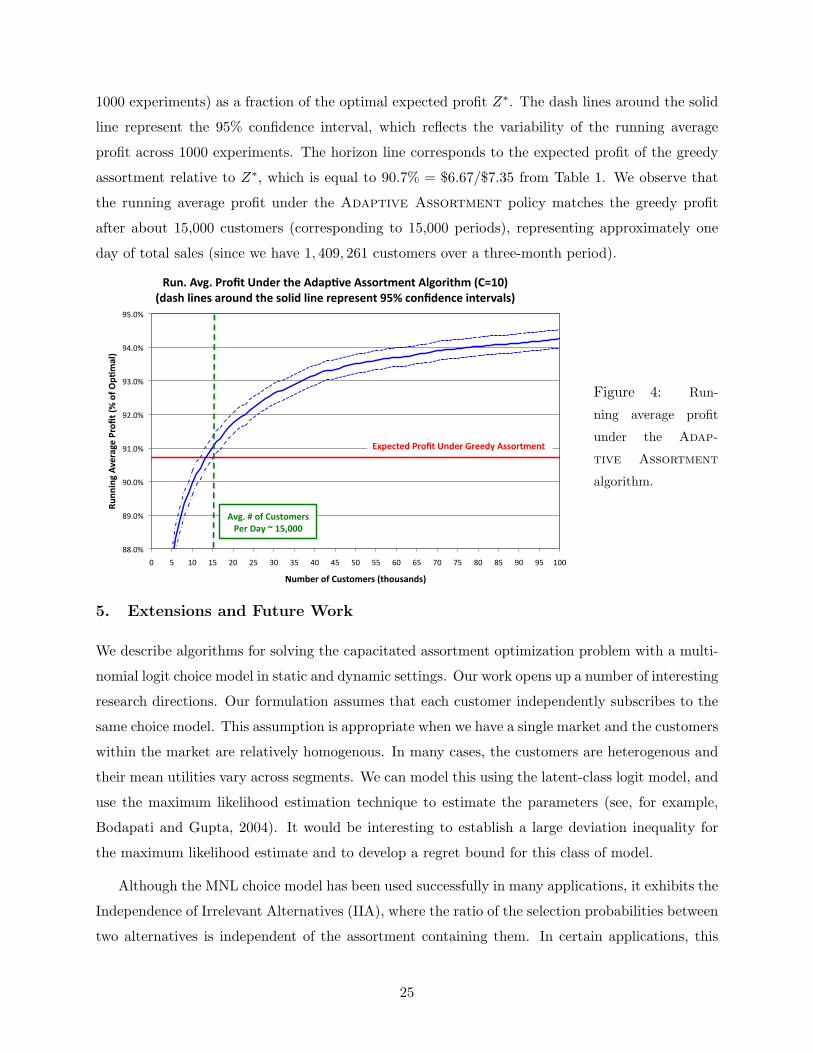
assortment relative to Z∗, which is equal to 90.7% = $6.67/$7.35 from Table 1. We observe that

the running average profit under the Adaptive Assortment policy matches the greedy profit

after about 15,000 customers (corresponding to 15,000 periods), representing approximately one

day of total sales (since we have 1, 409, 261 customers over a three-month period).

88.0%

89.0%

90.0%

91.0%

92.0%

93.0%

94.0%

95.0%

0 5 10 15 20 25 30 35 40 45 50 55 60 65 70 75 80 85 90 95 100

Runn

ingAverageProfit(%

ofO

p5mal)

NumberofCustomers(thousands)

Run.Avg.ProfitUndertheAdap5veAssortmentAlgorithm(C=10)(dashlinesaroundthesolidlinerepresent95%confidenceintervals)

ExpectedProfitUnderGreedyAssortment

Avg.#ofCustomersPerDay~15,000

Figure 4: Run-

ning average profit

under the Adap-

tive Assortment

algorithm.

5. Extensions and Future Work

We describe algorithms for solving the capacitated assortment optimization problem with a multi-

nomial logit choice model in static and dynamic settings. Our work opens up a number of interesting

research directions. Our formulation assumes that each customer independently subscribes to the

same choice model. This assumption is appropriate when we have a single market and the customers

within the market are relatively homogenous. In many cases, the customers are heterogenous and

their mean utilities vary across segments. We can model this using the latent-class logit model, and

use the maximum likelihood estimation technique to estimate the parameters (see, for example,

Bodapati and Gupta, 2004). It would be interesting to establish a large deviation inequality for

the maximum likelihood estimate and to develop a regret bound for this class of model.

Although the MNL choice model has been used successfully in many applications, it exhibits the

Independence of Irrelevant Alternatives (IIA), where the ratio of the selection probabilities between

two alternatives is independent of the assortment containing them. In certain applications, this

25

property may not be consistent with the actual customer choice behavior. Rusmevichientong et al.

(2009) has partially extended the solution technique developed in this paper to the nested logit

choice model, which is one of the most popular extensions of the MNL model that alleviates the IIA

property (McFadden, 1981). Under this model, the products are partitioned into groups. Although

products within the same group still exhibit the IIA property, the likelihood of choosing products

from two different groups depends on the assortment containing them, providing a potentially more

realistic model of customer choice behavior. In this case, the assortment A(λ) defined in Equation

(4) corresponds to the optimal solution of a sum-of-ratio optimization problem, which is NP-hard

and we must resort to approximation methods to compute A(λ). We believe that the structural

properties developed in this paper can be extended to this model as well. For our DVD dataset,

we might apply the nested logit model by grouping the DVDs based on their genre. However,

estimating the parameters in the nested logit can be complicated because the likelihood function

is not concave and approximation methods are required (see, for example, Silberhorn et al., 2008).

Our model also assumes that the cost of changing an assortment from one customer to the

next is negligible. This assumption is reasonable in the online setting where the cost of changing

the ads or product recommendations on the web page is minimal. However, in settings where

there are significant costs associated with switching product assortments, our model might not be

appropriate. In addition, we implicitly assume that we have enough supply of each product to

ignore all inventory considerations. Incorporating inventory constraints is an exciting direction for

future research.

Acknowledgement

The authors would like to thank Candi Yano for her helpful comments and suggestions on the

earlier draft of our manuscript, which inspired us to consider the multinomial logit choice model.

We are grateful for all of her help. We would like to thank Mike Todd for insightful comments

on linear algebra and for pointers to implementations of the Golden Ratio Search and Newton-

Raphson algorithms, Yinyu Ye for helpful discussions on the problem, and Miao Song for all of her

help with the BIOGEME software. We also want to thank Costis Maglaras for helpful discussions

about the applications of the MNL model during the first author’s visit to the Columbia Graduate

School of Business. Finally, we are grateful for Garrett van Ryzin, the associated editor, and the

three referees for their thoughtful and detailed comments on the earlier version of the manuscripts;

their suggestions greatly improve the quality and the presentation of our work. We also want

to thank the second referee for encouraging us to improve our estimated logit choice model in

Section 4, enabling us to discover the price per disc variable that turns out to be important in

26

explaining the customer purchase patterns. We are grateful for all of his/her suggestions. This

research is supported in part by the National Science Foundation through grants DMS-0732196,

CMMI-0746844, CMMI-0621433, CMMI-0727640, CCF-0635121, and CCF-0832782.

References

Anantharam, V., P. Varaiya, and J. Walrand. 1987a. Asymptotically efficient adaptive allocation rules for themulti-armed bandit problem with multiple plays, Part I: I.I.D. rewards. IEEE Transactions on AutomaticControl AC-32 (11): 968–976.

Anantharam, V., P. Varaiya, and J. Walrand. 1987b. Asymptotically efficient adaptive allocation rules forthe multi-armed bandit problem with multiple plays, Part II : Markovian rewards. IEEE Transactions onAutomatic Control AC-32 (11): 977–982.

Anderson, S., A. de Palma, and J. F. Thisse. 1992. Discrete choice theory of product differentiation. Cam-bridge, MA: MIT Press.

Auer, P., N. Cesa-Bianchi, and F. P. 2002. Finite-time analysis of the multiarmed bandit problem. MachineLearning 47:235–256.

Ben-Akiva, M., and S. Lerman. 1985. Discrete choice analysis: Theory and application to travel demand.Cambridge, MA: MIT Press.

Bierlaire, M. 2003. BIOGEME: A Free Package For the Estimation of Discrete Choice Models. In Proceedingsof the 3rd Swiss Transportation Research Conference. Ascona, Switzerland.

Bodapati, A. V., and S. Gupta. 2004. The recoverability of segmentation structure from store-level aggre-gation data. Journal of Marketing Research 41:351–364.

Caro, F., and J. Gallien. 2007. Dynamic assortment with demand learning for seasonal consumer goods.Management Science 53 (2): 276–292.

Cover, T. M., and J. A. Thomas. 2006. Elements of information theory. Wiley.

Gallego, G., G. Iyengar, R. Phillips, and A. Dubey. 2004. Managing flexible products on a network. WorkingPaper, Columbia University.

Kok, A. G., M. Fisher, and R. Vaidyanathan. 2008. Assortment planning: Review of literature and industrypractice. In Retail Supply Chain Management: Springer.

Kunnumkal, S., and H. Topaloglu. 2008. A refined deterministic linear program for the network revenuemanagement problem with customer choice behavior. Naval Research Logistics 55 (6): 563–580.

Lai, T. L., and H. Robbins. 1985. Asymptotically efficient adaptive allocation rules. Advances in AppliedMathematics 6 (1): 4–22.

Levi, R., R. O. Roundy, and D. B. Shmoys. 2007. Provably near-optimal sampling-based algorithms forstochastic inventory control models. Mathematics of Operations Research 32 (4): 821–838.

Liu, Q., and G. J. van Ryzin. 2008. On the choice-based linear programming model for network revenuemanagement. Manufacturing and Service Operations Management 10 (2): 288–310.

27

Mahajan, S., and G. J. van Ryzin. 1998. Retail inventories and consumer choice. In Quantitative Modelsfor Supply Chain Management, ed. S. Tayur, R. Ganeshan, and M. Magazine, 491–551: Kluwer AcademicPublishers.

Mahajan, S., and G. J. van Ryzin. 2001. Stocking retail assortments under dynamic consumer substitution.Operations Research 49 (3): 334–351.

McFadden, D. 1981. Econometric models of probabilistic choice. In Structural Analysis of Discrete Data:MIT Press.

Megiddo, N. 1979. Combinatorial optimization with rational objective functions. Mathematics of OperationsResearch 4 (4): 414–424.

Press, W. H., S. A. Teukolsky, and W. T. V. et al.. 1999. Numerical recipes in C, the art of scientificcomputing. Cambridge University Press.

Ratliff, R., B. V. Rao, C. P. Narayan, and K. Yellepeddi. 2007. A multi-flight recapture heuristic forestimating unconstrained demand from airline bookings. Journal of Revenue and Pricing Management 7(2): 153–171.

Rusmevichientong, P., Z.-J. M. Shen, and D. B. Shmoys. 2009. A PTAS for capacitated sum-of-ratiosoptimization. Operations Research Letters 37 (4): 230–238.

Saure, D., and A. Zeevi. 2008. Optimal dynamic assortment planning. Working Paper, Columbia GraduateSchool of Business.

Shapiro, A. 2003. Stochastic programming. In Handbook in Operations Research and Management Science.Elsevier.

Shen, Z.-J. M., and X. Su. 2007. Customer behavior modeling in revenue management and auctions: Areview and new research opportunities. Production and Operations Management 16 (6): 713–728.

Silberhorn, N., Y. Boztug, and L. Hildebrandt. 2008, 653. Estimation with the nested logit model: specifi-cations and software particularities. OR Spectrum 30 (4): 635.

Swamy, C., and D. B. Shmoys. 2005. Sampling-based approximation algorithms for multi-stage stochasticoptimization. In Proceedings of the 46th Annual IEEE Symposium on the Foundations of ComputerScience.

Talluri, K., and G. J. van Ryzin. 2004. Revenue management under a general discrete choice model ofconsumer behavior. Management Science 50 (1): 15–33.

Vulcano, G., G. J. van Ryzin, and R. Ratliff. 2008. Estimating primary demand for substitutable productsfrom sales transaction data. Working paper, Stern Business School.

Zhang, D., and D. Adelman. 2008. An approximate dynamic programming approach to network revenuemanagement with customer choice. To appear in Transportation Science.

28

A. Proof of Theorem 2.5

The proof of Theorem 2.5 makes use of the following lemmas. Recall that, under Assumption 2.1, the numberof intersection points K is exactly

(N+1

2

), and the StaticMNL algorithm maintains the following four pieces

of information associated with the interval(I (i`, j`) , I (i`+1, j`+1)

): 1) the ordering σ` =

(σ`1, . . . , σ

`N

)of

the lines h1(·), . . . , hN (·) from the highest to the smallest values, 2) the set G` corresponding to the firstC elements according to the ordering σ`, 3) the set B` of lines whose values have become negative, and 4)the assortment A` = G` \ B`. The first lemma (whose proof appears in Appendix A.1) provides a simplecharacterization of the ordering among intersection points among any three lines.

Lemma A.1. Under Assumption 2.1, for all 0 ≤ i < j < k ≤ N , one of the following conditions must hold:either I(i, j) < I(i, k) < I(j, k) or I(j, k) < I(i, k) < I(i, j).

For any ordering γ : {1, . . . , N} → {1, . . . , N}, x is adjacent to y under γ if∣∣γ−1(x)− γ−1(y)

∣∣ = 1. Thenext lemma characterizes the orderings σ` generated under the StaticMNL algorithm. The proof of thislemma appears in Appendix A.2.

Lemma A.2. Under Assumption 2.1, for each ` = 1, 2, . . . ,K, either σ` = σ`−1 or σ` is obtained bytransposing two adjacent items under σ`−1.

The next lemma shows that if a set G` (corresponding to the first C elements in the permutation σ`) isdistinct from all the previous sets, then one of its elements must be strictly smaller. The proof of this resultappears in Appendix A.3.

Lemma A.3. Under Assumption 2.1, for each ` = 1, 2, . . . ,K, if G` 6= G`−1, then G` is obtained from G`−1

by transposition between j` = σ`−1C and i` = σ`−1

C+1 with 0 < i` < j`, that is, G` =(G`−1 \ {j`}

)∪ {i`} and∑

`∈G` ` <∑`∈G`−1 ` .

The next lemma shows that the size of the assortments generated by the StaticMNL algorithm isnon-increasing. The proof appears in Appendix A.4.

Lemma A.4. Let θ denote the smallest index such that∣∣Aθ∣∣ < C. Then, Aθ = Aθ−1 \ {jθ}, and for all

` > θ, either A` = A`−1 or A` = A`−1 \ {j`} .

We are now ready to give a proof of Theorem 2.5.

Proof. To prove part (a) of Theorem 2.5, suppose that A` 6= A`−1. If∣∣A`∣∣ = C, it follows from Lemma

A.4 that ` < θ. This implies that A` = G` and A`−1 = G`−1. It follows from Lemma A.3 that A` =(A`−1 \ {j`}

)∪ {i`}. On the other hand, if

∣∣A`∣∣ < C, the desired result follows from Lemma A.4.

Lemma A.4 also shows that there are exactly C − 1 distinct non-empty assortments of size C − 1 orless, which establishes part (b) of Theorem 2.5. To complete the proof, it suffices to count the number ofdistinct assortments of size C. Note that if A` is an assortment of size C, it must be the case that A` = G`.Therefore, the number of distinct assortments of size C is bounded above by the number of distinct subsetsamong the sets G`.

Under Assumption 2.1, we know that, among h1(·), . . . , hN (·), each of the(N2

)pairs of lines will intersect

each other. Moreover, by Assumption 2.1, we have that σ0 = (N,N − 1, . . . , 2, 1), corresponding to the order

29

of hi(λ)’s at λ = −∞, and σK = (1, 2, . . . , N − 1, N) for λ = +∞. Note that∑`∈G0

`−∑`∈GK

` = {N + (N − 1) + · · ·+ (N − C + 1)} − {1 + 2 + · · ·+ C}

= NC − 2(1 + 2 + · · ·+ C − 1)− C = NC − C(C − 1)− C = C(N − C).

By Lemma A.3, whenever Gt is distinct from Gt−1, the total value∑`∈Gt ` is strictly less than

∑`∈Gt−1 `.

Thus, in addition to G0, there can be at most C(N − C) distinct subsets of G`’s. Therefore, the number ofdistinct subsets among G0, G1, . . . , GK is at most C(N − C) + 1. Thus, the maximum number of distinctnon-empty assortments is at most C(N −C) + 1 + (C − 1) = C(N −C + 1), which is the desired result.

A.1 Proof of Lemma A.1

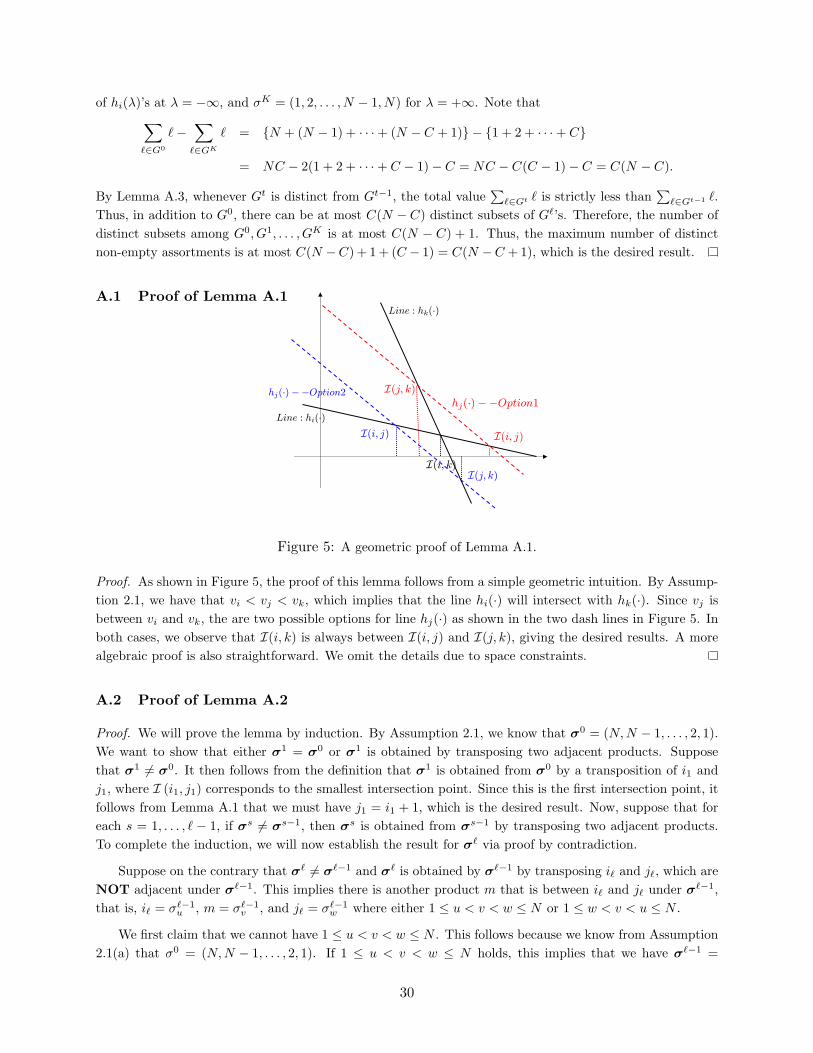
I(i, k)

hj(·)−−Option2hj(·)−−Option1

Line : hk(·)

Line : hi(·)

I(i, j) I(i, j)

I(j, k)

I(j, k)

Figure 5: A geometric proof of Lemma A.1.

Proof. As shown in Figure 5, the proof of this lemma follows from a simple geometric intuition. By Assump-tion 2.1, we have that vi < vj < vk, which implies that the line hi(·) will intersect with hk(·). Since vj isbetween vi and vk, the are two possible options for line hj(·) as shown in the two dash lines in Figure 5. Inboth cases, we observe that I(i, k) is always between I(i, j) and I(j, k), giving the desired results. A morealgebraic proof is also straightforward. We omit the details due to space constraints.

A.2 Proof of Lemma A.2

Proof. We will prove the lemma by induction. By Assumption 2.1, we know that σ0 = (N,N − 1, . . . , 2, 1).We want to show that either σ1 = σ0 or σ1 is obtained by transposing two adjacent products. Supposethat σ1 6= σ0. It then follows from the definition that σ1 is obtained from σ0 by a transposition of i1 andj1, where I (i1, j1) corresponds to the smallest intersection point. Since this is the first intersection point, itfollows from Lemma A.1 that we must have j1 = i1 + 1, which is the desired result. Now, suppose that foreach s = 1, . . . , ` − 1, if σs 6= σs−1, then σs is obtained from σs−1 by transposing two adjacent products.To complete the induction, we will now establish the result for σ` via proof by contradiction.

Suppose on the contrary that σ` 6= σ`−1 and σ` is obtained by σ`−1 by transposing i` and j`, which areNOT adjacent under σ`−1. This implies there is another product m that is between i` and j` under σ`−1,that is, i` = σ`−1

u , m = σ`−1v , and j` = σ`−1

w where either 1 ≤ u < v < w ≤ N or 1 ≤ w < v < u ≤ N .

We first claim that we cannot have 1 ≤ u < v < w ≤ N . This follows because we know from Assumption2.1(a) that σ0 = (N,N − 1, . . . , 2, 1). If 1 ≤ u < v < w ≤ N holds, this implies that we have σ`−1 =

30

(. . . , i`, . . . ,m, . . . , j`, . . .) . Since i` < j` and the transpositions in all of the previous iterations involveadjacent items by induction, it must be the case that i` and j` have switched places once before, that is, wemust have already encountered the intersection point I(i`, j`) in the earlier iterations. Contradiction!

So, we have 1 ≤ w < v < u ≤ N , which implies that σ`−1 = (. . . , j`, . . . ,m, . . . , i`, . . .) . By construction,we know that i` < j`. Thus, there are three cases to consider for the value of m.

Case 1: m < i` < j`. In this case, m is smaller than i` but appears earlier in the ordering σ`−1. Sinceσ0 = (N,N − 1, . . . , 2, 1) and all previous transpositions involve adjacent items by induction, it must be thecase that i` and m interchange their positions in the earlier iteration, implying that I(m, i`) < I(i`, j`). Itthus follows from Lemma A.1 that

I(m, i`) < I(m, j`) < I(i`, j`),

implying that we must have already encountered the intersection point I(m, j`) before this iteration. Byinduction, this means that m and j` should have interchanged their places and we must have m before j`(note that m ≥ 1). This contradicts our definition of σ`−1!

Case 2: i` < m < j`. In this case, it follows from Lemma A.1 that either

I(i`,m) < I(i`, j`) < I(m, j`) OR I(m, j`) < I(i`, j`) < I(i`,m).

We will show that either one of the above condition will lead to a contradiction. Suppose that I(i`,m) <I(i`, j`) < I(m, j`). This implies that we must have encountered the intersection point I(i`,m) before thecurrent iteration. Therefore, by induction, m and i` should have switched places and we must have m afteri` in σ`−1. This again contradicts our definition of σ`−1! Now, suppose that I(m, j`) < I(i`, j`) < I(i`,m).Then, we must have encountered the intersection point I(m, j`) before the current iteration. Therefore,by induction, m and j` should have switched places and we must have m before j` in σ`−1. This againcontradicts our definition of σ`−1!

Case 3: i` < j` < m. The proof for this case is similar to Case 1 and we omit the details.

Thus, all three cases lead to contradictions. Therefore, it must be the case that σ` is obtained from σ`−1

by transposing two adjacent products. This completes the induction.

A.3 Proof of Lemma A.3

Proof. By definition, if G` 6= G`−1, it must be the case that we encounter an intersection point I (i`, j`) with0 < i` < j`. In this case, σ` is obtained from σ`−1 by transposition of i` and j`. Moreover, we know fromLemma A.2 that i` is adjacent to j` under σ`−1. Note that G` and G`−1 correspond to the first C elementsfor the ordering σ` and σ`−1, respectively. Thus, in order for G` to be different from G`−1, it must be thecase that either 1) σ`−1

C = j` and σ`−1C+1 = i`, or 2) σ`−1

C = i` and σ`−1C+1 = j`.

We will first show that option 2) is not feasible. Recall that under Assumption 2.1, we have σ0 =(N,N − 1, . . . , 2, 1). Since i` < j` and every transposition only occur between adjacent items (by LemmaA.2), if σ`−1

C = i` and σ`−1C+1 = j`, then it must be the case that i` and j` have interchanged places

before; that is, we have already encountered the intersection point I (i`, j`) in the earlier iterations. Thisis a contradiction! Therefore, we can only have σ`−1

C = j` and σ`−1C+1 = i`. In this case, we have G` =(

G`−1 \ {j`})∪ {i`}, which implies that

∑`∈G` `−

∑`∈G`−1 ` = i` − j` < 0, which is the desired result.

31

A.4 Proof of Lemma A.4

Proof. Since∣∣A0∣∣ = C, θ ≥ 1. We will first show that Aθ = Aθ−1 \ {jθ}. By definition, the set Aθ is created

when we encounter the θth intersection point I (iθ, jθ). We claim that we must have iθ = 0. Suppose onthe contrary that we have 0 < iθ < jθ. In this case, Bθ = Bθ−1. Thus, for

∣∣Aθ∣∣ < C =∣∣Aθ−1

∣∣, it must bethe case that Gθ 6= Gθ−1. It follows from Lemma A.3 that Gθ is obtained from Gθ−1 by transposition ofjθ = σθ−1

C and iθ = σθ−1C+1 with 0 < iθ < jθ. Since

∣∣Aθ∣∣ < C, it follows that Bθ 3 iθ, which implies that wemust have already encountered the intersection I (0, iθ) earlier. By Lemma A.1,

I (0, iθ) < I (0, jθ) < I (iθ, jθ) ,

which implies that the intersection point I(0, jθ) appeared before the current iteration, and thus, Bθ−1 3 jθ,which implies that

∣∣Aθ−1∣∣ < C. Contradiction! Therefore, we must have iθ = 0. Then, we know that

σθ = σθ−1, Gθ = Gθ−1, and Bθ = Bθ−1 ∪ {jθ}. Since∣∣Aθ−1

∣∣ = C >∣∣Aθ∣∣, Gθ−1 ∩ Bθ−1 = ∅ and

Gθ ∩Bθ 6= ∅. Since only jθ is added to the set Bθ−1, we have Gθ ∩Bθ = {jθ}, and therefore, Aθ = Gθ \Bθ =Gθ \ {jθ} = Gθ−1 \ {jθ} = Aθ−1 \ {jθ}, which is the desired result.

To complete the proof of Lemma A.4, consider any ` > θ. Let r =∣∣A`−1

∣∣. Since ` > θ, we have thatr < C. By the definition, σ`−1 =

(σ`−1

1 , . . . , σ`−1N

)represent the ordering of the lines h1(·), . . . , hN (·) during

the interval(I (i`−1, jj−1) , I (i`, j`)

)with

hσ`−11

(I (i`, j`)) ≥ hσ`−12

(I (i`, j`)) ≥ · · · ≥ hσ`−1N

(I (i`, j`)) (11)

Since G`−1 ={σ`−1

1 , . . . , σ`−1C

}, A`−1 = G`−1 \B`−1, and

∣∣A`−1∣∣ = r < C, it follows from the above ordering

thathσ`−1

r(I (i`, j`)) ≥ 0 > hσ`−1

r+1(I (i`, j`)) ≥ · · · ≥ hσ`−1

N(I (i`, j`)) ,

and B`−1 ={σ`−1r+1, σ

`−1r+2, . . . , σ

`−1N

}.

We will show that either A` = A`−1 or A` = A`−1 \ {j`}. Consider the `th intersection point I (i`, j`).There are two cases to consider: i` = 0 and i` ≥ 1. Suppose that i` = 0. Then, we claim that j` = σ`−1

r . SinceB`−1 =

{σ`−1r+1, σ

`−1r+2, . . . , σ

`−1N

}, we know that j` ∈

{σ`−1

1 , . . . , σ`−1r

}. If, on the contrary, j` = σ`−1

k wherek < r, this means that I

(0, σ`−1

k

)< I

(0, σ`−1

r

); that is, the value associated with the line hσ`−1

rremains non-

negative. However, by the ordering in (11), it must be the case that 0 > hσ`−1k

(I (i`, j`)) ≥ hσ`−1r

(I (i`, j`)).Contradiction! Therefore, j` = σ`−1

r , which implies that A` = A`−1 \{σ`−1r

}, which is the desired result.

On the other hand, suppose that i` ≥ 1. In this case, we have B` = B`−1. We claim that we musteither have {i`, j`} ⊂ B` or {i`, j`} ⊂

(B`)c; that is, either both elements are in B` or both are not.

This will show that A` = A`−1, which is the desired result. To prove this, note that since 0 < i` < j`,it follows from Lemma A.1 that either I(0, i`) < I(0, j`) < I(i`, j`) or I(i`, j`) < I(0, j`) < I(0, i`). IfI(0, i`) < I(0, j`) < I(i`, j`) holds, then the intersection points I(0, i`) and I(0, j`) appear in the earlieriterations, implying that {i`, j`} ⊂ B`. On the other hand, if I(i`, j`) < I(0, j`) < I(0, i`), then i` /∈ B` andj` /∈ B`.

B. Proof of Lemma 2.7

Let r =(√

5− 1)/2 denote the golden ratio and let WGRS =

⌈2(log T )/β4

⌉. Since the classical Golden

Ratio search reduces the size of the target set by factor of r in each iteration, the maximum number ofiterations is at most dlog |A| / log(1/r)e, where |A| denotes the number of assortments in the sequence A.

32

For k = 1, . . . , dlog |A| / log(1/r)e, let 1 ≤ ak < bk < ck < dk ≤ |A| denote the 4 indices associatedwith the kth iteration of the golden search algorithm. In the kth iteration, we consider the assortmentsAak , Aak+1, . . . , Adk , and we compare the assortment Abk and Ack based on their average profits. If theaverage profit of Abk is larger than that of Ack , the resulting target set for the next iteration is Aak , . . . , Ack .Otherwise, the new target set will be Abk , . . . , Adk . Let Bk denote the event that resulting target set afterthe kth iteration does not contain the optimal assortment, that is, we made an error in the kth iteration. Wewish to show that Pr {Bk} ≤ 2ke−β

4WGRS/2

Let q ∈ {1, . . . , |A|} denote the index of the optimal assortment. Consider the first iteration where wecompare the average profit of Ab1 and Ac1 . Let Y b11 , . . . , Y b1WGRS

denote the observed profit associated withthe selections of the WGRS customers who were offered the assortment Ab1 . Similarly, let Y c11 , . . . , Y c1WGRS

denote the observed profits associated with Ac1 . Note that if b1 ≤ q ≤ c1, then Pr{B1} = 0 because theresulting target set will always contain the optimal assortment, regardless of the outcome of the comparison.So, suppose that q < b1. Then, we know from Theorem 2.6 that f(Ab1)− f(Ac1) > β2. Using the fact thatE[Y b1i

]= f(Ab1) and E [Y c1i ] = f(Ac1) for all 1 ≤ i ≤ WGRS , we can bound the probability of error in the

first iteration as follows

Pr {B1} = Pr

{1

WGRS

WGRS∑i=1

Y b1i <1

WGRS

WGRS∑i=1

Y c1i

}

≤ Pr

{1

WGRS

WGRS∑i=1

(Y c1i − f(Ac1)) +1

WGRS

WGRS∑i=1

(f(Ab1)− Y b1i

)> f(Ab1)− f(Ac1)

}

≤ Pr

{1

WGRS

WGRS∑i=1

(Y c1i − f(Ac1)) +1

WGRS

WGRS∑i=1

(f(Ab1)− Y b1i

)> β2

}

≤ Pr

{1

WGRS

WGRS∑i=1

(Y c1i − f(Ac1)) >β2

2

}+ Pr

{1

WGRS

WGRS∑i=1

(f(Ab1)− Y b1i

)>β2

2

}≤ 2e−β

4WGRS/2 ,

where the last inequality follows from the classical Chernoff-Hoeffding Inequality and the fact that w` ≤ 1for all `. The argument for the case where q > c1 is exactly the same. To get a bound on Pr{B2}, note thatPr{B2} = Pr{B2|B1}Pr{B1}+ Pr{B2|Bc1}Pr{Bc1} ≤ Pr{B1}+ Pr{B2|Bc1}. Using exactly the same argumentas above, we can show that Pr{B2|Bc1} ≤ 2e−β

4WGRS/2. Therefore, Pr{B2} ≤ 2(

2e−β4WGRS/2

). Repeated

applications show that Pr {Bk} ≤ 2ke−β4WGRS/2.

To determine an upper bound on the regret after T periods, we note that the total number of samplesthat we used is at most

WGRS ·(⌈

log |A|log(1/r)

⌉+ 3)≤ 4WGRS ·

⌈log |A|

log(1/r)

⌉,

where the factor of 3 reflects the fact that the standard Golden Ratio search starts with 4 points in thefirst iteration and adds one additional search point in subsequent iterations. The maximum expected regretincurred from these samples is at most 4 ·WGRS ·

⌈log|A|

log(1/r)

⌉. because max` w` ≤ 1. Moreover, if we correctly

identify the optimal assortment at the end of the search, the regret will be zero thereafter. Thus, themaximum expected regret after we conclude the search algorithm is at most

T · Pr{Bdlog|A|/ log(1/r)e

}≤ 2T

⌈log |A|

log(1/r)

⌉e−β

4WGRS/2,

where the right hand side follows from the upper bound on the error probability. Using the definition of

33

WGRS , we have the following upper bound on the expected regret after T periods:

4 ·WGRS ·⌈

log |A|log(1/r)

⌉+ 2T

⌈log |A|

log(1/r)

⌉e−β

4WGRS/2

≤ 4(

2 log Tβ4

+ 1)(

log |A|log(1/r)

+ 1)

+ 2(

log |A|log(1/r)

+ 1)

= 4(

2 log Tβ4

+ 1)(

log(|A| /r)log(1/r)

)+ 2

(log(|A| /r)log(1/r)

)=

8 log(|A| /r)β4 log(1/r)

log T + 6log(|A| /r)log(1/r)

,

and the desired result follows from the fact that 1/r ≤ 2 and 1/ log(1/r) ≤ 2.079, and from Theorem 2.5which shows that |A| ≤ C(N − C + 1) ≤ N2.

C. Proof of Theorem 3.2

Proof. By the union bound and the fact that ε ≥ min{ε, β/3}, we have that

Pr{

maxS∈E

{max

{i,j}⊆S:i 6=j

∣∣∣I(i, j)− Iij(m,S)∣∣∣ ,max

i∈S

∣∣∣θi (S)− Θi (m,S)∣∣∣} > ε

}≤

∑S∈E

Pr{

max{i,j}⊆S:i6=j

∣∣∣I(i, j)− Iij(m,S)∣∣∣ > ε OR max

i∈S

∣∣∣θi (S)− Θi (m,S)∣∣∣ > min{ε, β/3}

}≤

∑S∈E

Pr{

maxi∈S

∣∣∣θi (S)− Θi (m,S)∣∣∣ > εβ2/12

},

where the last inequality follows from the fact that the event

max{i,j}⊆S:i 6=j

∣∣∣I(i, j)− Iij(m,S)∣∣∣ > ε OR max

i∈S

∣∣∣θi (S)− Θi (m,S)∣∣∣ > min{ε, β/3}

is a subset of the eventmaxi∈S

∣∣∣θi (S)− Θi (m,S)∣∣∣ > εβ2/12 .

To see this, note that min{ε, β/3} ≥ εβ2/12 because 0 < β < 1. If maxi∈S∣∣∣θi (S)− Θi (m,S)

∣∣∣ > min{ε, β/3},then the result is trivially true.

On the other hand, suppose that

maxi∈S

∣∣∣θi (S)− Θi (m,S)∣∣∣ ≤ min{ε, β/3} and max

{i,j}⊆S:i 6=j

∣∣∣I(i, j)− Iij(m,S)∣∣∣ > ε .

It follows from the definition of β in Equation (8) that for any (i, j) 6= (s, t), |I(i, j)− I(s, t)| ≥ β,and for any i 6= j and S ∈ E , |θi(S)− θj(S)| ≥ β. This implies that for each {i, j} ⊆ S and i 6= j,∣∣∣Θi (m,S)− Θj (m,S)

∣∣∣ ≥ β/3. Therefore,

∣∣∣∣∣ θi(S)θi(S)− θj(S)

− Θi(m,S)

Θi(m,S)− Θj(m,S)

∣∣∣∣∣ ≤ 2 max`∈S∣∣∣θ`(S)− Θ`(m,S)

∣∣∣(θi(S)− θj(S))

(Θi(m,S)− Θj(m,S)

)≤ 6

β2max`∈S

∣∣∣θ`(S)− Θ`(m,S)∣∣∣ ,

and it follows from the definition of I(i, j) and Iij(m,S) and the fact that max` w` ≤ 1 that∣∣∣I(i, j)− Iij(m,S)∣∣∣ ≤ 12

β2max`∈S

∣∣∣θ`(S)− Θ`(m,S)∣∣∣ .

34

Since {i, j} ⊆ S is arbitrary, we have that

ε < max{i,j}⊆S:i6=j

∣∣∣I(i, j)− Iij(m,S)∣∣∣ ≤ 12

β2max`∈S

∣∣∣θ`(S)− Θ`(m,S)∣∣∣ ,

which once again implies that maxi∈S∣∣∣θi (S)− Θi (c, S)

∣∣∣ > εβ2/12 .

Note that for each i ∈ S, Θi(c, S) is simply the average of c independent Bernoulli random variableswith parameter θi(S). Therefore, it follows from the standard Chernoff-Hoeffding Inequality that

Pr{∣∣∣θi (S)− Θi (c, S)

∣∣∣ > εβ2/12}≤ 2 e−2c(εβ2/12)2 = 2 e−c ε

2 β4/72 ,

and thus, Pr{

maxi∈S∣∣∣θi (S)− Θi (c, S)

∣∣∣ > εβ2/12}≤ 2Ce−c ε

2 β4/72. Putting everything together and using

the fact that |E| ≤ 5(N/C)2, we have that

Pr{

maxS∈E

{max

{i,j}⊆S:i6=j

∣∣∣I(i, j)− Iij(m,S)∣∣∣ ,max

i∈S

∣∣∣θi (S)− Θi (c, S)∣∣∣} > ε

}≤ 10N2

Ce−c ε

2 β4/72 ,

which is the desired result.

D. Proof of Theorem 3.4

Since w` ≤ 1 for all `, the regret incurred in each period is bounded above by 1. Consider an arbitrarycycle m. We incurred a total regret of |E| during the exploration phase of cycle m. At the end of theexploration phase, if A(m) = A, then the regret incurred from the Sampling-based GRS algorithm duringthe exploitation phase is bounded above by a1(logN) log Vm by Lemma 2.7. On the other hand, if A(m) 6= A,we incurred a total regret of at most Vm. Thus, the total regret incurred during the mth cycle is boundedabove by

|E|+ Vm Pr{A(m) 6= A

}+ a1(logN) log Vm ≤ |E|+

10N2

Ce−(α−β6/288)m + a1α(logN)m ,

where the inequality follows from Theorem 3.3 and the fact that Vm = beαmc ≤ eαm. Therefore, the totalcumulative regret after M cycles (corresponding to |E|M +

∑Mm=1 Vm periods) is bounded above by

Regret

(|E|M +

M∑m=1

Vm,AA

)≤ |E|M + a1α logN

M∑m=1

m+10N2

C

M∑m=1

e−(α−β6/288)m

≤ |E|M + a1α(logN)M2 +10N2/C

1− e−(α−β6/288)

Consider an arbitrary time period T . Let M0 =⌈

log Tα

⌉. Note that the total time periods after M0 cycles

is at least T because

M0 |E|+M0∑m=1

Vm = M0 |E|+M0∑m=1

beαmc = M0(|E| − 1) +M0∑m=1

eαm ≥ eαM0 ≥ T .

Since the cumulative regret is nondecreasing, it follows that

Regret (T,AA) ≤ Regret

(|E|M0 +

M0∑m=1

Vm,AA

)

≤ |E|M0 + a1α(logN)M20 +

10N2/C

1− e−(α−β6/288)≤ a2N

2 log2 T ,

for some constant a2 that depends on C, v, and w. The last inequality above follows from the fact that|E| = O(N2).

35