fast estimation of multinomial logit models: r package mnlogit
TRANSCRIPT
JSS Journal of Statistical SoftwareNovember 2016, Volume 75, Issue 3. doi: 10.18637/jss.v075.i03
Fast Estimation of Multinomial Logit Models:
R Package mnlogit
Asad Hasan
Sentrana Inc.Wang Zhiyu
Carnegie Mellon UniversityAlireza S. Mahani
Sentrana Inc.
Abstract
We present the R package mnlogit for estimating multinomial logistic regression mod-els, particularly those involving a large number of categories and variables. Comparedto existing software, mnlogit offers speedups of 10–50 times for modestly sized problemsand more than 100 times for larger problems. Running in parallel mode on a multicoremachine gives up to 4 times additional speedup on 8 processor cores. mnlogit achievesits computational efficiency by drastically speeding up computation of the log-likelihoodfunction’s Hessian matrix through exploiting structure in matrices that arise in intermedi-ate calculations. This efficient exploitation of intermediate data structures allows mnlogit
to utilize system memory much more efficiently, such that for most applications mnlogit
requires less memory than comparable software by a factor that is proportional to thenumber of model categories.
Keywords: logistic regression, multinomial logit, discrete choice, large scale, parallel, econo-metrics.
1. Introduction
Multinomial logit regression models, the multiclass extension of binary logistic regression, havelong been used in econometrics in the context of modeling discrete choice (McFadden 1974;Bhat 1995; Train 2003) and in machine learning as a linear classification technique (Hastie,Tibshirani, and Friedman 2009) for tasks such as text classification (Nigam, Lafferty, andMcCallum 1999). Training these models presents the computational challenge of having tocompute a large number of coefficients which increases linearly with the number of categoriesand the number of variables. Despite the potential for multinomial logit models to becomecomputationally expensive to estimate, they have an intrinsic structure which can be exploitedto dramatically speedup estimation. Our objective in this paper is twofold: First we describehow to exploit this structure to optimize computational efficiency, and second, to present an
2 mnlogit: Fast Estimation of Multinomial Logit Models in R
implementation of our ideas in our R (R Core Team 2016) package mnlogit (Hasan, Zhiyu,and Mahani 2015) which is available from the Comprehensive R Archive Network (CRAN) athttps://CRAN.R-project.org/package=mnlogit.
An older method of dealing with the computational issues involved in estimating large scalemultinomial logistic regressions has been to approximate it as a series of binary logistic re-gressions (Begg and Gray 1984). In fact the R package mlogitBMA (Sevcikova and Raftery2013) implements this idea as the first step in applying Bayesian model averaging to multi-nomial logit data. Large scale logistic regressions can, in turn, be tackled by a number ofadvanced optimization algorithms (Komarek and Moore 2005; Lin, Weng, and Keerthi 2008).A number of recent R packages have focused on slightly different aspects of estimating reg-ularized multinomial logistic regressions. For example, package glmnet (Friedman, Hastie,and Tibshirani 2010) is optimized for obtaining the entire L1-regularized paths and uses thecoordinate descent algorithm with “warm starts”, package maxent (Jurka 2012) is intendedfor large text classification problems which typically have very sparse data and the packagepmlr (Colby, Lee, Lewinger, and Bull 2010) which penalizes the likelihood function with theJeffrey’s prior to reduce first order bias and works well for small to medium sized datasets.There are also R packages which estimate plain (unregularized) multinomial regression mod-els. Some examples are the VGAM package (Yee 2010), the multinom function in packagennet (Venables and Ripley 2002) and the package mlogit (Croissant 2013).
Of all the R packages previously described, mlogit is the most versatile in the sense that ithandles many data types and extensions of multinomial logit models (such as nested logit,heteroskedastic logit, etc.). This is especially important in econometric applications, whichare motivated by the utility maximization principle (McFadden 1974), where one encountersdata which depends upon both the observation instance and the choice class. Our packagemnlogit provides the ability of handling these general data types while adding the advantageof very quick computations. This work is motivated by our own practical experience of theimpossibility of being able to estimate large scale multinomial logit models using existingsoftware.
In mnlogit we perform maximum likelihood estimation (MLE) using the Newton-Raphson(NR) method. We speed up the NR method by exploiting structure and sparsity in inter-mediate data matrices to achieve very fast computations of the Hessian of the log-likelihoodfunction. This overcomes the NR method’s well known weakness of incurring very highper-iteration cost, compared to algorithms from the quasi-Newton family (Nocedal 1992,1990). Indeed classical NR estimations of multinomial logit models (usually of the iterativelyreweighted least square family) have been slow for this very reason. On a single processor ourmethods have allowed us to achieve speedups of 10–50 times compared to mlogit on modest-sized problems while performing identical computations. In parallel mode1, mnlogit affordsthe user an additional speedup of 2–4 times while using up to 8 processor cores.
We provide a simple formula-based interface for specifying a varied menu of models to mnlogit.Section 2 illustrates aspects of the formula interface, the expected data format and the preciseinterpretations of variables in mnlogit. To make the fullest use of mnlogit we suggest that theuser understands the simple R example worked out over the course of this section. Section 3and Appendix A contain the details of our estimation procedure, emphasizing the ideas that
1Requires mnlogit to be compiled with OpenMP (OpenMP Architecture Review Board 2015) support (usu-ally present by default with most R installations, except on Mac OS X).
Journal of Statistical Software 3
underlie the computational efficiency we achieve in mnlogit. In Section 4 we present theresults of our numerical experiments in benchmarking and comparing mnlogit’s performancewith other packages while Appendix C has a synopsis of our timing methods. Finally Section 5concludes with a short discussion and a promising idea for future work.
2. On using mnlogit
The data for multinomial logit models may vary with both the choice makers (“individuals”)and the choices themselves. Besides, the modeler may prefer model coefficients that may (ormay not) depend on choices. In mnlogit we try to keep the user interface as minimal as possiblewithout sacrificing flexibility. We follow the interface of the mlogit function in package mlogit.This section describes the mnlogit user interface, emphasizing data preparation requirementsand model specification via an enhanced formula interface. To start, we load the packagemnlogit in an R session:
R> library("mnlogit")
2.1. Data preparation
mnlogit accepts data in the “long” format which requires that if there are K choices, thenthere are K rows of data for each individual (see also Section 1.1 of the mlogit vignette). Hereis a snapshot from data in the “long” format on choice of recreational fishing mode made by1182 individuals:
R> data("Fish", package = "mnlogit")
R> head(Fish, 8)
mode income alt price catch chid
1.beach FALSE 7083.332 beach 157.930 0.0678 1
1.boat FALSE 7083.332 boat 157.930 0.2601 1
1.charter TRUE 7083.332 charter 182.930 0.5391 1
1.pier FALSE 7083.332 pier 157.930 0.0503 1
2.beach FALSE 1250.000 beach 15.114 0.1049 2
2.boat FALSE 1250.000 boat 10.534 0.1574 2
2.charter TRUE 1250.000 charter 34.534 0.4671 2
2.pier FALSE 1250.000 pier 15.114 0.0451 2
In the Fish data, there are 4 choices ("beach", "boat", "charter", "pier") available to eachindividual: labeled by the chid (chooser ID). The price and catch column show, respectively,the cost of a fishing mode and (in unspecified units) the expected amount of fish caught. Animportant point here is that this data varies both with individuals and the fishing mode. Theincome column reflects the income level of an individual and does not vary between choices.Notice that the snapshot shows this data for two individuals.
The actual choice made by an individual, the “response” variable, is shown in the columnmode. mnlogit requires that the data contain a column with exactly two categories whose levels
4 mnlogit: Fast Estimation of Multinomial Logit Models in R
can be coerced to integers by as.numeric(). The greater of these integers is automaticallytaken to mean TRUE.
The only other column strictly mandated by mnlogit is one listing the names of choices (likecolumn alt in the Fish data). However if the data frame is an ‘mlogit.data’ class object,then this column may be omitted. In such cases mnlogit can query the index attribute of an‘mlogit.data’ object to figure out the information contained in the alt column.
2.2. Model parametrization
Multinomial logit models have a solid basis in the theory of discrete choice models. The centralidea in these discrete models lies in the “utility maximization principle” which states thatindividuals choose the alternative, from a finite, discrete set, which maximizes a scalar valuecalled “utility”. Discrete choice models presume that the utility is completely deterministic forthe individual, however modelers can only model a part of the utility (the “observed” part).Stochasticity entirely arises from the unobserved part of the utility. Different assumptionsabout the probability distribution of the unobserved utility give rise to various choice modelslike multinomial logit, nested logit, multinomial probit, GEV (generalized extreme value),mixed logit etc. Multinomial logit models, in particular, assume that the unobserved utilityis i.i.d. and follows a Gumbel distribution (see Train 2003, particularly Chapters 3 and 5, fora full discussion).
We consider that the observed part of the utility for the ith individual choosing the kthalternative is given by:
Uik = ξk + ~Xi · ~βk + ~Yik · ~γk + ~Zik · ~α. (1)
Here Latin letters (X, Y , Z) stand for design matrices while Greek letters (ξ, α, β, γ) standfor coefficients. The parameter ξk is called the intercept. For many practical applications,variables in multinomial logit models can be naturally grouped into two types:
• Individual specific variables ~Xi which do not vary between choices (e.g., income ofindividuals in the Fish data of Section 2.1).
• Alternative specific variables ~Yik and ~Zik which vary with alternative and may alsodiffer, for the same alternative, between individuals (e.g., the amount of fish caught inthe Fish data: column catch).
In mnlogit we model these two types of variables with three types of coefficients:
1. Individual specific variables with alternative specific coefficients ~Xi · ~βk.
2. Alternative specific variables with alternative independent coefficients ~Zik · ~α.
3. Alternative specific variables with alternative specific coefficients ~Yik · ~γk.
The vector notation denotes that more than one variable of each type may be used to builda model. For example in the fish data we may choose both the price and catch with eitheralternative independent coefficients (the ~α) or with alternative specific coefficients (the ~γk).
Due to the principle of utility maximization, only differences between utilities are meaningful.This implies that the multinomial logit model cannot determine absolute utility. We must
Journal of Statistical Software 5
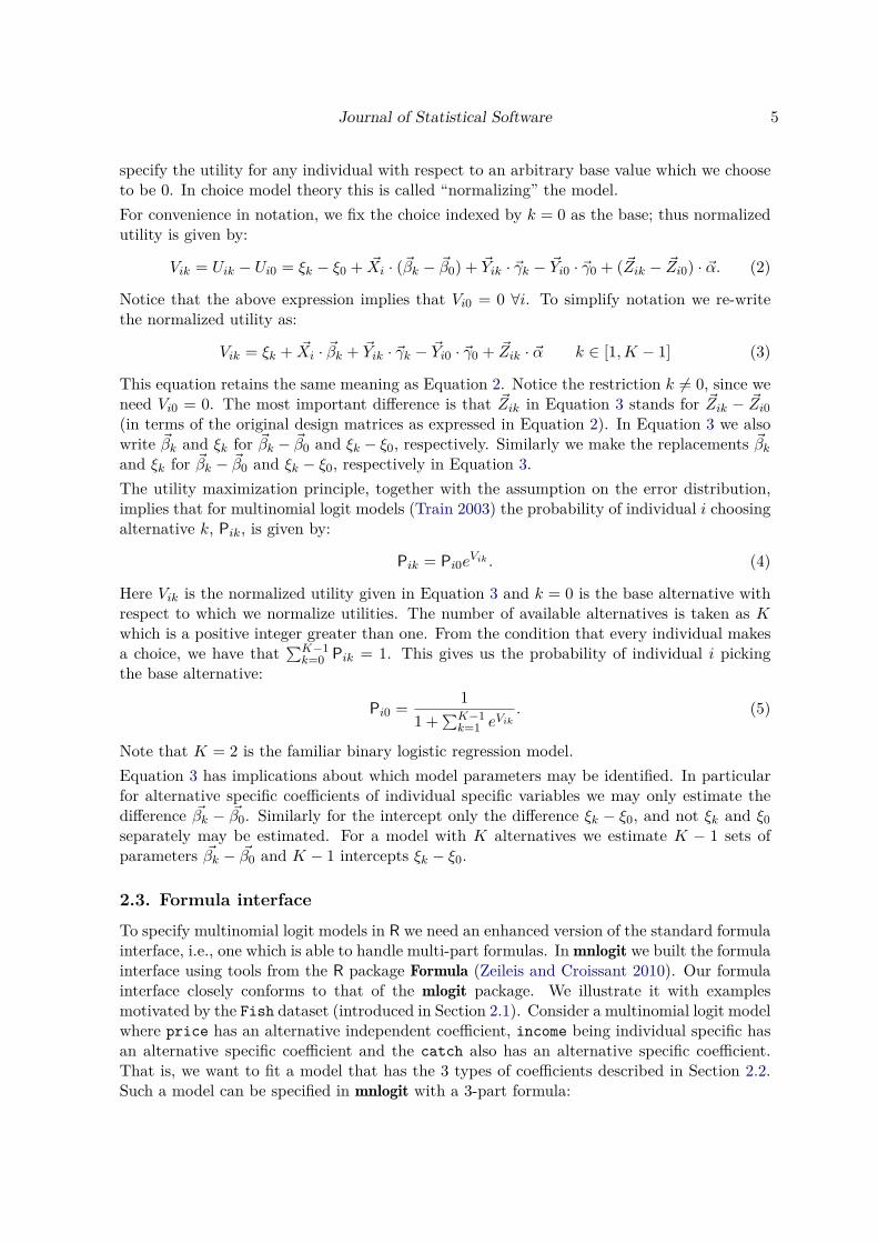
specify the utility for any individual with respect to an arbitrary base value which we chooseto be 0. In choice model theory this is called “normalizing” the model.
For convenience in notation, we fix the choice indexed by k = 0 as the base; thus normalizedutility is given by:
Vik = Uik − Ui0 = ξk − ξ0 + ~Xi · (~βk − ~β0) + ~Yik · ~γk − ~Yi0 · ~γ0 + (~Zik − ~Zi0) · ~α. (2)
Notice that the above expression implies that Vi0 = 0 ∀i. To simplify notation we re-writethe normalized utility as:
Vik = ξk + ~Xi · ~βk + ~Yik · ~γk − ~Yi0 · ~γ0 + ~Zik · ~α k ∈ [1, K − 1] (3)
This equation retains the same meaning as Equation 2. Notice the restriction k 6= 0, since weneed Vi0 = 0. The most important difference is that ~Zik in Equation 3 stands for ~Zik − ~Zi0
(in terms of the original design matrices as expressed in Equation 2). In Equation 3 we alsowrite ~βk and ξk for ~βk − ~β0 and ξk − ξ0, respectively. Similarly we make the replacements ~βk
and ξk for ~βk − ~β0 and ξk − ξ0, respectively in Equation 3.
The utility maximization principle, together with the assumption on the error distribution,implies that for multinomial logit models (Train 2003) the probability of individual i choosingalternative k, Pik, is given by:
Pik = Pi0eVik . (4)
Here Vik is the normalized utility given in Equation 3 and k = 0 is the base alternative withrespect to which we normalize utilities. The number of available alternatives is taken as Kwhich is a positive integer greater than one. From the condition that every individual makesa choice, we have that
∑K−1k=0 Pik = 1. This gives us the probability of individual i picking
the base alternative:
Pi0 =1
1 +∑K−1
k=1 eVik
. (5)
Note that K = 2 is the familiar binary logistic regression model.
Equation 3 has implications about which model parameters may be identified. In particularfor alternative specific coefficients of individual specific variables we may only estimate thedifference ~βk − ~β0. Similarly for the intercept only the difference ξk − ξ0, and not ξk and ξ0
separately may be estimated. For a model with K alternatives we estimate K − 1 sets ofparameters ~βk − ~β0 and K − 1 intercepts ξk − ξ0.
2.3. Formula interface
To specify multinomial logit models in R we need an enhanced version of the standard formulainterface, i.e., one which is able to handle multi-part formulas. In mnlogit we built the formulainterface using tools from the R package Formula (Zeileis and Croissant 2010). Our formulainterface closely conforms to that of the mlogit package. We illustrate it with examplesmotivated by the Fish dataset (introduced in Section 2.1). Consider a multinomial logit modelwhere price has an alternative independent coefficient, income being individual specific hasan alternative specific coefficient and the catch also has an alternative specific coefficient.That is, we want to fit a model that has the 3 types of coefficients described in Section 2.2.Such a model can be specified in mnlogit with a 3-part formula:
6 mnlogit: Fast Estimation of Multinomial Logit Models in R
R> fm <- formula(mode ~ price | income | catch)
By default, the intercept is included, it can be omitted by inserting a -1 or 0 anywhere inthe formula. The following formulas specify the same model with omitted intercept:
R> fm <- formula(mode ~ price | income - 1 | catch)
R> fm <- formula(mode ~ price | income | catch - 1)
R> fm <- formula(mode ~ 0 + price | income | catch)
We can omit any group of variables from the model by placing a 1 as a placeholder:
R> fm <- formula(mode ~ 1 | income | catch)
R> fm <- formula(mode ~ price | 1 | catch)
R> fm <- formula(mode ~ price | income | 1)
R> fm <- formula(mode ~ price | 1 | 1)
R> fm <- formula(mode ~ 1 | 1 | price + catch)
When the meaning is unambiguous, an omitted group of variables need not have a placeholder.The following formulas represent the same model where price and catch are modeled withalternative independent coefficients and the intercept is included:
R> fm <- formula(mode ~ price + catch | 1 | 1)
R> fm <- formula(mode ~ price + catch | 1)
R> fm <- formula(mode ~ price + catch)
2.4. Using package mnlogit
The complete mnlogit function synopsis is:
mnlogit(formula, data, choiceVar = NULL, maxiter = 50, ftol = 1e-6,
gtol = 1e-6, weights = NULL, ncores = 1, na.rm = TRUE, print.level = 0,
linDepTol = 1e-6, start = NULL, alt.subset = NULL, ...)
We have described the formula and data arguments in previous sections while others areexplained in the man page, only the linDepTol argument needs further elaboration. Dataused to estimate the model must satisfy certain necessary conditions so that the Hessianmatrix, computed during Newton-Raphson estimation, has full rank (more about this inAppendix B). In mnlogit we use the R built-in function qr, with its argument tol set tolinDepTol, to check for linear dependencies. If collinear columns are detected in the data,using the criteria discussed in Appendix B, then some are removed so that the remainingcolumns are linearly independent.
We now illustrate the practical usage of mnlogit and some of its methods by a simple example.Consider the model specified by the formula:
R> fm <- formula(mode ~ price | income | catch)
This model has:

Journal of Statistical Software 7
• One alternative independent coefficient price corresponding to ~α.
• Two alternative specific coefficients income and intercept corresponding to ~βk. Wetreat the intercept as the coefficient corresponding to an alternative specific “variable”consisting of a vector of ones.
• One alternative specific coefficient catch corresponding to ~γk.
In the Fish data the number of alternatives K = 4, so the number of coefficients in the abovemodel is:
• One coefficient for a variable that may vary with individuals and alternatives, corre-sponding to ~α.
• 2 × (K − 1) = 6, alternative specific coefficients for individual specific variables (notethat we have subtracted 1 from the number of alternatives because after normalizationthe base choice coefficient cannot be identified), corresponding to ~βk.
• 1 × K = 4 alternative specific coefficients for variables which may vary with individualsand alternatives, corresponding to ~γk.
Thus the total number of coefficients in this model is 1 + 6 + 4 = 11.
We call the function mnlogit to fit the model using the Fish dataset on two processor cores.
R> fit <- mnlogit(fm, Fish, ncores = 2)
R> class(fit)
[1] "mnlogit"
For ‘mnlogit’ class objects we provide a number of S3 methods. Besides the usual methodsassociated with R objects (coef, print, summary and predict), we also provide methodssuch as: residuals, fitted, logLik, vcov, df.residual, update and terms. In addition,the returned object (here fit) can be queried for details of the estimation process by:
R> print(fit, what = "eststat")
-------------------------------------------------------------
Maximum likelihood estimation using the Newton-Raphson method
-------------------------------------------------------------
Number of iterations: 7
Number of linesearch iterations: 10
At termination:
Gradient norm = 2.09e-06
Diff between last 2 loglik values = 0
Stopping reason: Succesive loglik difference < ftol (1e-06).
Total estimation time (sec): 0.036
Time for Hessian calculations (sec): 0.005 using 2 processors.
8 mnlogit: Fast Estimation of Multinomial Logit Models in R
The estimation process terminates when any one of the three conditions maxiter, ftol orgtol is met. In case one runs into numerical singularity problems during the Newton itera-tions, we recommend relaxing ftol or gtol to obtain a suitable estimate. The plain Newtonmethod has a tendency to overshoot extrema. In mnlogit we have included a “line search”(one dimensional minimization along the Newton direction) which avoids this problem andensures convergence (Nocedal and Wright 2000).
As a convenience, the print method may be invoked to query an ‘mnlogit’ object for thenumber and type of model coefficients.
R> print(fit, what = "modsize")
Number of observations in data = 1182
Number of alternatives = 4
Intercept turned: ON
Number of parameters in model = 11
# individual specific variables = 2
# choice specific coeff variables = 1
# individual independent variables = 1
Finally there is provision for hypothesis testing. We provide the function hmftest to performthe Hausman-McFadden test for IIA (independence of irrelevant alternatives), which is thecentral hypothesis underlying multinomial logit models (Train 2003, Chapter 3). Three func-tions to test for hypotheses, applicable to any model estimated by the maximum likelihoodmethod, are also provided:
• Function lrtest to perform the likelihood ratio test.
• Function waldtest to perform the Wald test.
• Function scoretest to perform the Rao score test.
The intent of these tests is succinctly described in Section 6 “Tests” of the mlogit packagevignette and we shall not repeat it here. We encourage the interested user to consult thehelp page for any of these functions in the usual way, for example the lrtest help may beaccessed by:
R> library("mnlogit")
R> ?lrtest
Functions hmftest and scoretest are adapted from code in the mlogit package, while lrtest
and waldtest are built using tools in the R package lmtest (Zeileis and Hothorn 2002).
3. Estimation algorithm
In mnlogit we employ maximum likelihood estimation (MLE) to compute model coefficientsand use the Newton-Raphson method to solve the optimization problem. The Newton-Raphson method is well established for maximizing the logistic family log-likelihoods (Hastie
Journal of Statistical Software 9
et al. 2009; Train 2003). However direct approaches of computing the Hessian of the multi-nomial logit model log-likelihood function have deleterious effects on the computer time andmemory required. We present an alternate approach which exploits the structure of the inter-mediate data matrices that arise in Hessian calculation to achieve the same computation muchfaster while using drastically less memory. Our approach also allows us to optimally paral-lelize Hessian computation and maximize the use of BLAS (basic linear algebra subprograms)Level 3 functions, providing an additional factor of speedup.
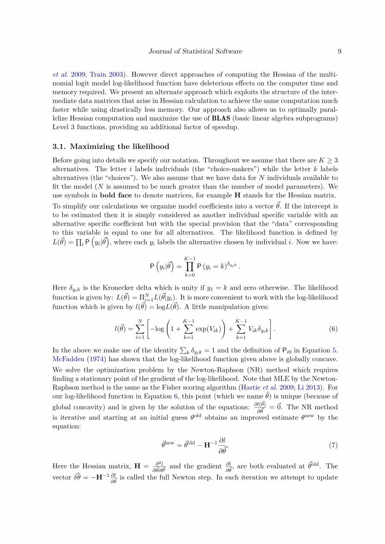
3.1. Maximizing the likelihood
Before going into details we specify our notation. Throughout we assume that there are K ≥ 3alternatives. The letter i labels individuals (the “choice-makers”) while the letter k labelsalternatives (the “choices”). We also assume that we have data for N individuals available tofit the model (N is assumed to be much greater than the number of model parameters). Weuse symbols in bold face to denote matrices, for example H stands for the Hessian matrix.
To simplify our calculations we organize model coefficients into a vector ~θ. If the intercept isto be estimated then it is simply considered as another individual specific variable with analternative specific coefficient but with the special provision that the “data” correspondingto this variable is equal to one for all alternatives. The likelihood function is defined by
L(~θ) =∏
i P
(
yi|~θ)
, where each yi labels the alternative chosen by individual i. Now we have:
P
(
yi|~θ)
=K−1∏
k=0
P (yi = k)δyik .
Here δyik is the Kronecker delta which is unity if y1 = k and zero otherwise. The likelihood
function is given by: L(~θ) = ΠNi=1L(~θ|yi). It is more convenient to work with the log-likelihood
function which is given by l(~θ) = logL(~θ). A little manipulation gives:
l(~θ) =N∑
i=1
[
−log
(
1 +K−1∑
k=1
exp(Vik)
)
+K−1∑
k=1
Vikδyik
]
. (6)
In the above we make use of the identity∑
k δyik = 1 and the definition of Pi0 in Equation 5.McFadden (1974) has shown that the log-likelihood function given above is globally concave.
We solve the optimization problem by the Newton-Raphson (NR) method which requiresfinding a stationary point of the gradient of the log-likelihood. Note that MLE by the Newton-Raphson method is the same as the Fisher scoring algorithm (Hastie et al. 2009; Li 2013). Forour log-likelihood function in Equation 6, this point (which we name θ̂) is unique (because of
global concavity) and is given by the solution of the equations: ∂l(~θ)
∂~θ= ~0. The NR method
is iterative and starting at an initial guess θold obtains an improved estimate θnew by theequation:
~θnew = ~θold − H−1 ∂l
∂~θ. (7)
Here the Hessian matrix, H = ∂2l
∂~θ∂~θ′and the gradient ∂l
∂~θ, are both evaluated at ~θold. The
vector ~δθ = −H−1 ∂l
∂~θis called the full Newton step. In each iteration we attempt to update
10 mnlogit: Fast Estimation of Multinomial Logit Models in R
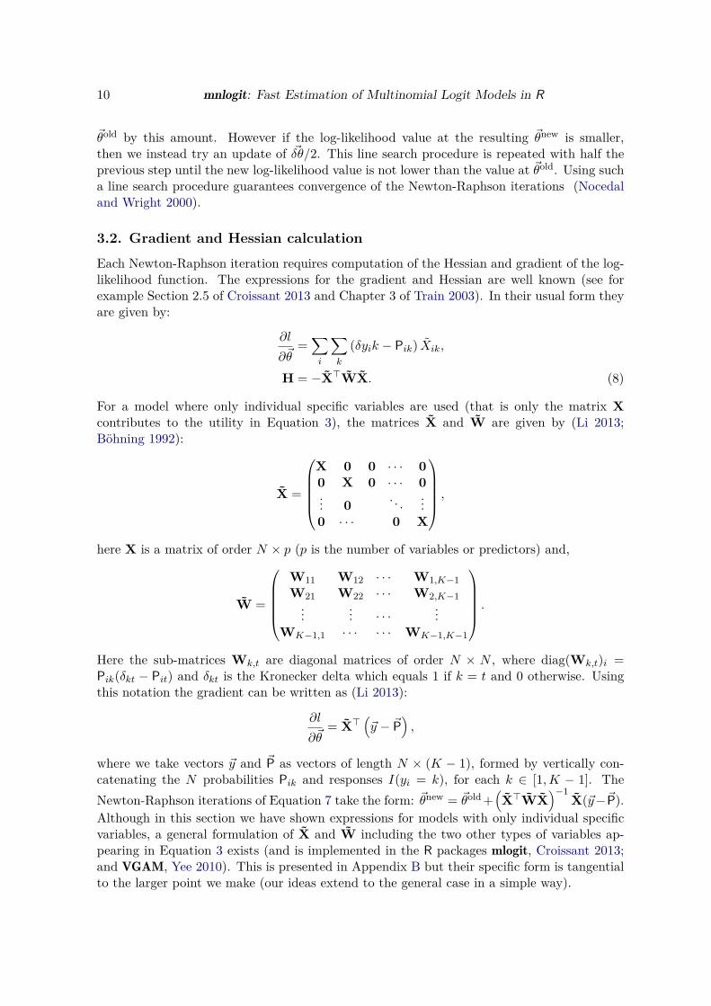
~θold by this amount. However if the log-likelihood value at the resulting ~θnew is smaller,then we instead try an update of ~δθ/2. This line search procedure is repeated with half theprevious step until the new log-likelihood value is not lower than the value at ~θold. Using sucha line search procedure guarantees convergence of the Newton-Raphson iterations (Nocedaland Wright 2000).
3.2. Gradient and Hessian calculation
Each Newton-Raphson iteration requires computation of the Hessian and gradient of the log-likelihood function. The expressions for the gradient and Hessian are well known (see forexample Section 2.5 of Croissant 2013 and Chapter 3 of Train 2003). In their usual form theyare given by:
∂l
∂~θ=∑
i
∑
k
(δyik − Pik) X̃ik,
H = −X̃⊤W̃X̃. (8)
For a model where only individual specific variables are used (that is only the matrix X
contributes to the utility in Equation 3), the matrices X̃ and W̃ are given by (Li 2013;Böhning 1992):
X̃ =
X 0 0 · · · 0
0 X 0 · · · 0... 0
. . ....
0 · · · 0 X
,
here X is a matrix of order N × p (p is the number of variables or predictors) and,
W̃ =
W11 W12 · · · W1,K−1
W21 W22 · · · W2,K−1...
... · · ·...
WK−1,1 · · · · · · WK−1,K−1
.
Here the sub-matrices Wk,t are diagonal matrices of order N × N , where diag(Wk,t)i =Pik(δkt − Pit) and δkt is the Kronecker delta which equals 1 if k = t and 0 otherwise. Usingthis notation the gradient can be written as (Li 2013):
∂l
∂~θ= X̃⊤
(
~y − ~P)
,
where we take vectors ~y and ~P as vectors of length N × (K − 1), formed by vertically con-catenating the N probabilities Pik and responses I(yi = k), for each k ∈ [1, K − 1]. The
Newton-Raphson iterations of Equation 7 take the form: ~θnew = ~θold +(
X̃⊤W̃X̃)−1
X̃(~y−~P).
Although in this section we have shown expressions for models with only individual specificvariables, a general formulation of X̃ and W̃ including the two other types of variables ap-pearing in Equation 3 exists (and is implemented in the R packages mlogit, Croissant 2013;and VGAM, Yee 2010). This is presented in Appendix B but their specific form is tangentialto the larger point we make (our ideas extend to the general case in a simple way).
Journal of Statistical Software 11
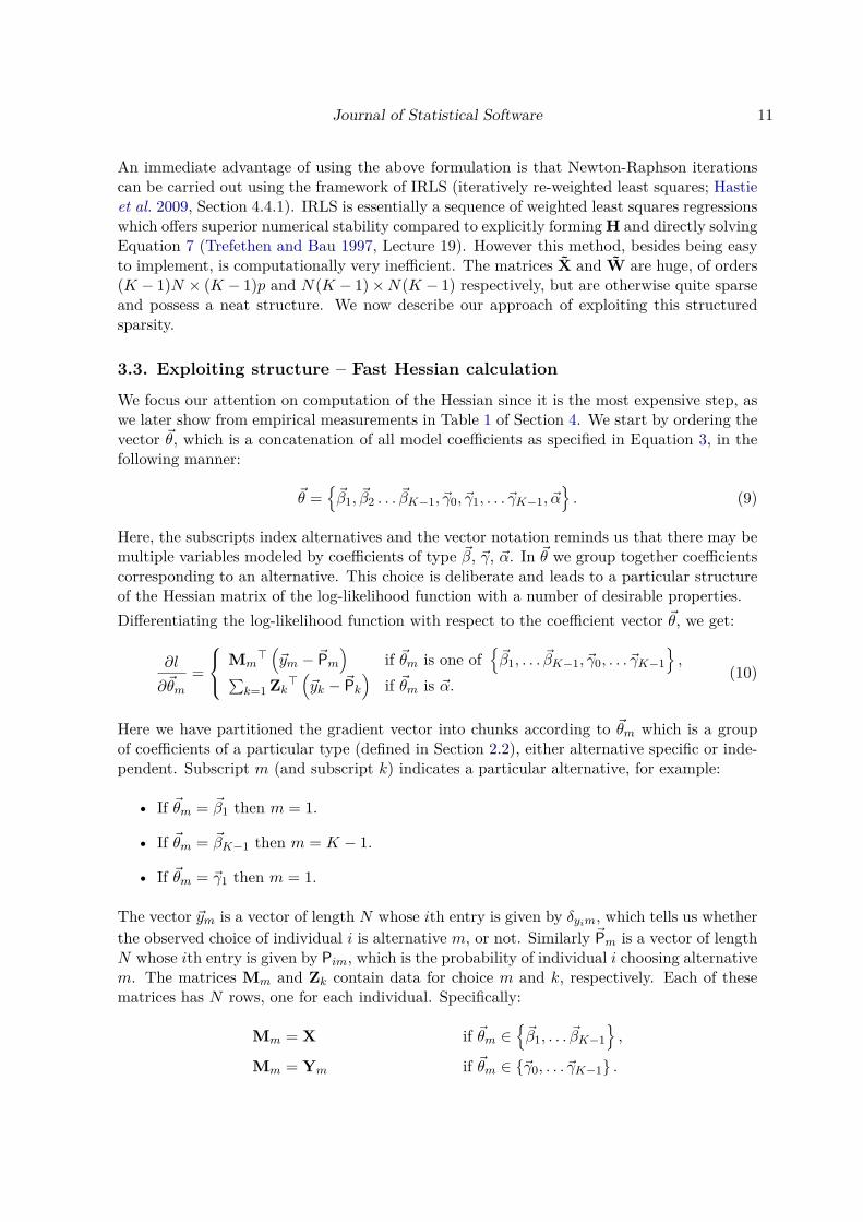
An immediate advantage of using the above formulation is that Newton-Raphson iterationscan be carried out using the framework of IRLS (iteratively re-weighted least squares; Hastieet al. 2009, Section 4.4.1). IRLS is essentially a sequence of weighted least squares regressionswhich offers superior numerical stability compared to explicitly forming H and directly solvingEquation 7 (Trefethen and Bau 1997, Lecture 19). However this method, besides being easyto implement, is computationally very inefficient. The matrices X̃ and W̃ are huge, of orders(K − 1)N × (K − 1)p and N(K − 1) × N(K − 1) respectively, but are otherwise quite sparseand possess a neat structure. We now describe our approach of exploiting this structuredsparsity.
3.3. Exploiting structure – Fast Hessian calculation
We focus our attention on computation of the Hessian since it is the most expensive step, aswe later show from empirical measurements in Table 1 of Section 4. We start by ordering thevector ~θ, which is a concatenation of all model coefficients as specified in Equation 3, in thefollowing manner:
~θ ={
~β1, ~β2 . . . ~βK−1, ~γ0, ~γ1, . . . ~γK−1, ~α}
. (9)
Here, the subscripts index alternatives and the vector notation reminds us that there may bemultiple variables modeled by coefficients of type ~β, ~γ, ~α. In ~θ we group together coefficientscorresponding to an alternative. This choice is deliberate and leads to a particular structureof the Hessian matrix of the log-likelihood function with a number of desirable properties.
Differentiating the log-likelihood function with respect to the coefficient vector ~θ, we get:
∂l
∂~θm
=
Mm⊤
(
~ym − ~Pm
)
if ~θm is one of{
~β1, . . . ~βK−1, ~γ0, . . . ~γK−1
}
,∑
k=1 Zk⊤
(
~yk − ~Pk
)
if ~θm is ~α.(10)
Here we have partitioned the gradient vector into chunks according to ~θm which is a groupof coefficients of a particular type (defined in Section 2.2), either alternative specific or inde-pendent. Subscript m (and subscript k) indicates a particular alternative, for example:
• If ~θm = ~β1 then m = 1.
• If ~θm = ~βK−1 then m = K − 1.
• If ~θm = ~γ1 then m = 1.
The vector ~ym is a vector of length N whose ith entry is given by δyim, which tells us whether
the observed choice of individual i is alternative m, or not. Similarly ~Pm is a vector of lengthN whose ith entry is given by Pim, which is the probability of individual i choosing alternativem. The matrices Mm and Zk contain data for choice m and k, respectively. Each of thesematrices has N rows, one for each individual. Specifically:
Mm = X if ~θm ∈{
~β1, . . . ~βK−1
}
,
Mm = Ym if ~θm ∈ {~γ0, . . . ~γK−1} .
12 mnlogit: Fast Estimation of Multinomial Logit Models in R
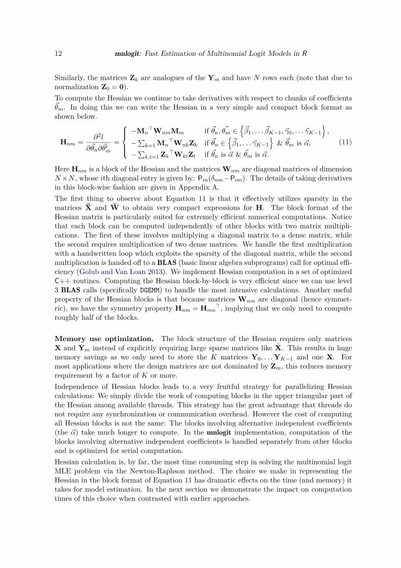
Similarly, the matrices Zk are analogues of the Ym and have N rows each (note that due tonormalization Z0 = 0).
To compute the Hessian we continue to take derivatives with respect to chunks of coefficients~θm. In doing this we can write the Hessian in a very simple and compact block format asshown below.
Hnm =∂2l
∂~θn∂~θ′m
=
−Mn⊤WnmMm if ~θn, ~θm ∈
{
~β1, . . . ~βK−1, ~γ0, . . . ~γK−1
}
,
−∑
k=1 Mn⊤WnkZk if ~θn ∈
{
~β1, . . . ~γK−1
}
& ~θm is ~α,
−∑
k,t=1 Zk⊤WktZt if ~θn is ~α & ~θm is ~α.
(11)
Here Hnm is a block of the Hessian and the matrices Wnm are diagonal matrices of dimensionN ×N , whose ith diagonal entry is given by: Pin(δnm −Pim). The details of taking derivativesin this block-wise fashion are given in Appendix A.
The first thing to observe about Equation 11 is that it effectively utilizes sparsity in thematrices X̃ and W̃ to obtain very compact expressions for H. The block format of theHessian matrix is particularly suited for extremely efficient numerical computations. Noticethat each block can be computed independently of other blocks with two matrix multipli-cations. The first of these involves multiplying a diagonal matrix to a dense matrix, whilethe second requires multiplication of two dense matrices. We handle the first multiplicationwith a handwritten loop which exploits the sparsity of the diagonal matrix, while the secondmultiplication is handed off to a BLAS (basic linear algebra subprograms) call for optimal effi-ciency (Golub and Van Loan 2013). We implement Hessian computation in a set of optimizedC++ routines. Computing the Hessian block-by-block is very efficient since we can use level3 BLAS calls (specifically DGEMM) to handle the most intensive calculations. Another usefulproperty of the Hessian blocks is that because matrices Wnm are diagonal (hence symmet-ric), we have the symmetry property Hnm = Hmn
⊤, implying that we only need to computeroughly half of the blocks.
Memory use optimization. The block structure of the Hessian requires only matricesX and Ym instead of explicitly requiring large sparse matrices like X̃. This results in hugememory savings as we only need to store the K matrices Y0, . . . YK−1 and one X. Formost applications where the design matrices are not dominated by Zm, this reduces memoryrequirement by a factor of K or more.
Independence of Hessian blocks leads to a very fruitful strategy for parallelizing Hessiancalculations: We simply divide the work of computing blocks in the upper triangular part ofthe Hessian among available threads. This strategy has the great advantage that threads donot require any synchronization or communication overhead. However the cost of computingall Hessian blocks is not the same: The blocks involving alternative independent coefficients(the ~α) take much longer to compute. In the mnlogit implementation, computation of theblocks involving alternative independent coefficients is handled separately from other blocksand is optimized for serial computation.
Hessian calculation is, by far, the most time consuming step in solving the multinomial logitMLE problem via the Newton-Raphson method. The choice we make in representing theHessian in the block format of Equation 11 has dramatic effects on the time (and memory) ittakes for model estimation. In the next section we demonstrate the impact on computationtimes of this choice when contrasted with earlier approaches.
Journal of Statistical Software 13
4. Benchmarking performance
For the purpose of performance profiling mnlogit code, we use simulated data generated usinga custom R function makeModel() sourced from simChoiceModel.R which is available in thepackage inside folder mnlogit/vignettes/ and in the supplementary files to this manuscript.Using simulated data we can easily vary problem size to study performance of the code – whichis our main intention here – and make comparisons to other packages. Our tests have beenperformed on a dual-socket, 64-bit Intel machine with 8 cores per socket which are clockedat 2.6 GHz2. R has been natively compiled on this machine using gcc with BLAS/LAPACK
support from single-threaded Intel MKL v11.0.
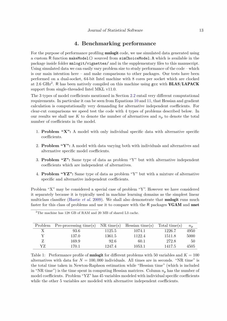
The 3 types of model coefficients mentioned in Section 2.2 entail very different computationalrequirements. In particular it can be seen from Equations 10 and 11, that Hessian and gradientcalculation is computationally very demanding for alternative independent coefficients. Forclear-cut comparisons we speed test the code with 4 types of problems described below. Inour results we shall use K to denote the number of alternatives and np to denote the totalnumber of coefficients in the model.
1. Problem “X”: A model with only individual specific data with alternative specificcoefficients.
2. Problem “Y”: A model with data varying both with individuals and alternatives andalternative specific model coefficients.
3. Problem “Z”: Same type of data as problem “Y” but with alternative independentcoefficients which are independent of alternatives.
4. Problem “YZ”: Same type of data as problem “Y” but with a mixture of alternativespecific and alternative independent coefficients.
Problem “X” may be considered a special case of problem “Y”. However we have consideredit separately because it is typically used in machine learning domains as the simplest linearmulticlass classifier (Hastie et al. 2009). We shall also demonstrate that mnlogit runs muchfaster for this class of problems and use it to compare with the R packages VGAM and nnet
2The machine has 128 GB of RAM and 20 MB of shared L3 cache.
Problem Pre-processing time(s) NR time(s) Hessian time(s) Total time(s) np
X 93.6 1125.5 1074.1 1226.7 4950Y 137.0 1361.5 1122.4 1511.8 5000Z 169.9 92.6 60.1 272.8 50
YZ 170.1 1247.4 1053.1 1417.5 4505
Table 1: Performance profile of mnlogit for different problems with 50 variables and K = 100alternatives with data for N = 100, 000 individuals. All times are in seconds. “NR time” isthe total time taken in Newton-Raphson estimation while “Hessian time” (which is includedin “NR time”) is the time spent in computing Hessian matrices. Column np has the number ofmodel coefficients. Problem “YZ” has 45 variables modeled with individual specific coefficientswhile the other 5 variables are modeled with alternative independent coefficients.
14 mnlogit: Fast Estimation of Multinomial Logit Models in R
which fit only this class of problems (see Appendix C). The “YZ” class of problems serves toillustrate a common use case of multinomial logit models in econometrics where the data mayvary with both individuals and alternatives while the coefficients are a mixture of alternativespecific and independent types (usually only a small fraction of variables are modeled withalternative independent coefficients).
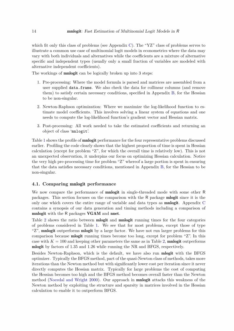
The workings of mnlogit can be logically broken up into 3 steps:
1. Pre-processing: Where the model formula is parsed and matrices are assembled from auser supplied data.frame. We also check the data for collinear columns (and removethem) to satisfy certain necessary conditions, specified in Appendix B, for the Hessianto be non-singular.
2. Newton-Raphson optimization: Where we maximize the log-likelihood function to es-timate model coefficients. This involves solving a linear system of equations and oneneeds to compute the log-likelihood function’s gradient vector and Hessian matrix.
3. Post-processing: All work needed to take the estimated coefficients and returning anobject of class ‘mnlogit’.
Table 1 shows the profile of mnlogit performance for the four representative problems discussedearlier. Profiling the code clearly shows that the highest proportion of time is spent in Hessiancalculation (except for problem “Z”, for which the overall time is relatively low). This is notan unexpected observation, it underpins our focus on optimizing Hessian calculation. Noticethe very high pre-processing time for problem “Z” whereof a large portion is spent in ensuringthat the data satisfies necessary conditions, mentioned in Appendix B, for the Hessian to benon-singular.
4.1. Comparing mnlogit performance
We now compare the performance of mnlogit in single-threaded mode with some other R
packages. This section focuses on the comparison with the R package mlogit since it is theonly one which covers the entire range of variable and data types as mnlogit. Appendix Ccontains a synopsis of our data generation and timing methods including a comparison ofmnlogit with the R packages VGAM and nnet.
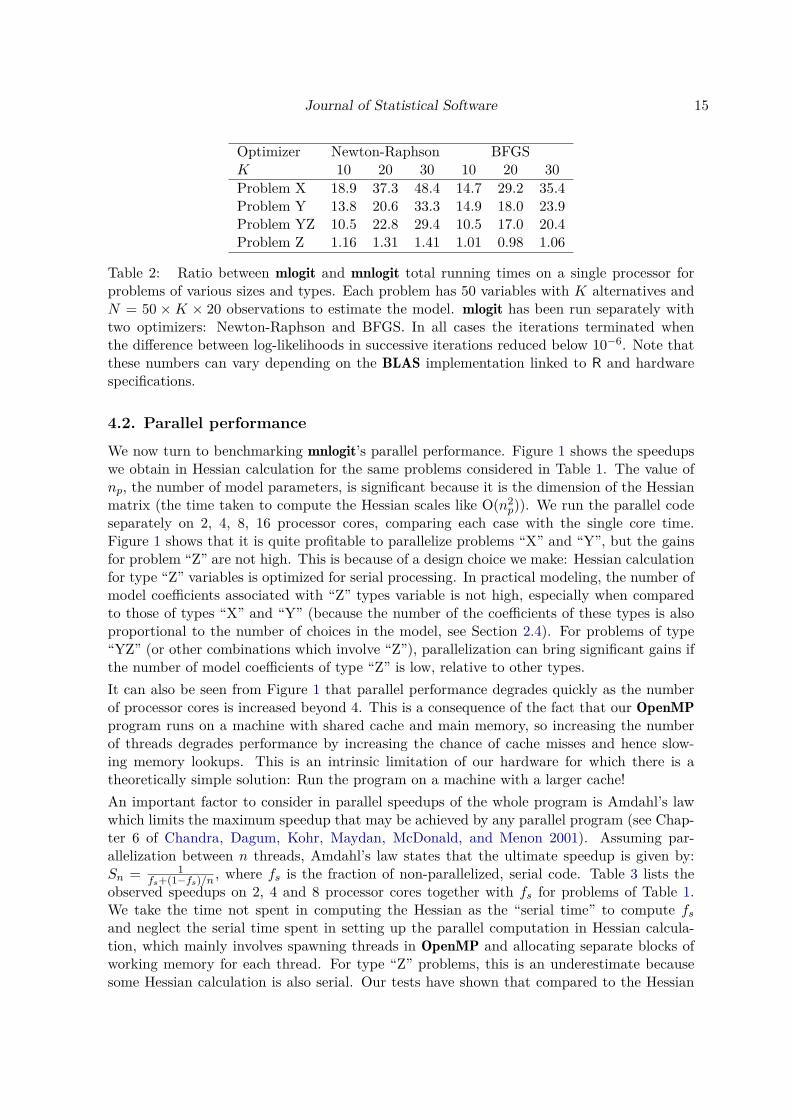
Table 2 shows the ratio between mlogit and mnlogit running times for the four categoriesof problems considered in Table 1. We see that for most problems, except those of type“Z”, mnlogit outperforms mlogit by a large factor. We have not run larger problems for thiscomparison because mlogit running times become too long, except for problem “Z”. In thiscase with K = 100 and keeping other parameters the same as in Table 2, mnlogit outperformsmlogit by factors of 1.35 and 1.26 while running the NR and BFGS, respectively.
Besides Newton-Raphson, which is the default, we have also run mlogit with the BFGSoptimizer. Typically the BFGS method, part of the quasi-Newton class of methods, takes moreiterations than the Newton method but with significantly lower cost per iteration since it neverdirectly computes the Hessian matrix. Typically for large problems the cost of computingthe Hessian becomes too high and the BFGS method becomes overall faster than the Newtonmethod (Nocedal and Wright 2000). Our approach in mnlogit attacks this weakness of theNewton method by exploiting the structure and sparsity in matrices involved in the Hessiancalculation to enable it to outperform BFGS.
Journal of Statistical Software 15
Optimizer Newton-Raphson BFGSK 10 20 30 10 20 30
Problem X 18.9 37.3 48.4 14.7 29.2 35.4Problem Y 13.8 20.6 33.3 14.9 18.0 23.9Problem YZ 10.5 22.8 29.4 10.5 17.0 20.4Problem Z 1.16 1.31 1.41 1.01 0.98 1.06
Table 2: Ratio between mlogit and mnlogit total running times on a single processor forproblems of various sizes and types. Each problem has 50 variables with K alternatives andN = 50 × K × 20 observations to estimate the model. mlogit has been run separately withtwo optimizers: Newton-Raphson and BFGS. In all cases the iterations terminated whenthe difference between log-likelihoods in successive iterations reduced below 10−6. Note thatthese numbers can vary depending on the BLAS implementation linked to R and hardwarespecifications.
4.2. Parallel performance
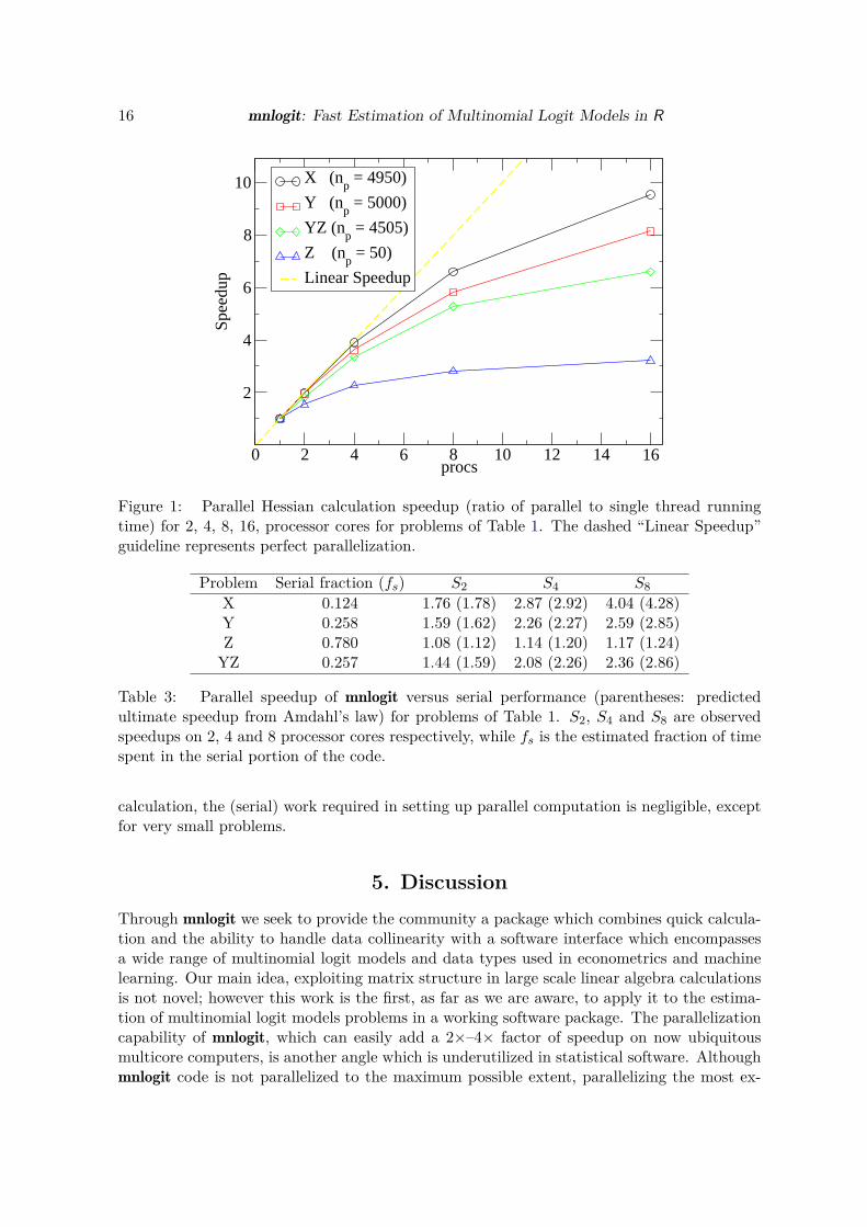
We now turn to benchmarking mnlogit’s parallel performance. Figure 1 shows the speedupswe obtain in Hessian calculation for the same problems considered in Table 1. The value ofnp, the number of model parameters, is significant because it is the dimension of the Hessianmatrix (the time taken to compute the Hessian scales like O(n2
p)). We run the parallel codeseparately on 2, 4, 8, 16 processor cores, comparing each case with the single core time.Figure 1 shows that it is quite profitable to parallelize problems “X” and “Y”, but the gainsfor problem “Z” are not high. This is because of a design choice we make: Hessian calculationfor type “Z” variables is optimized for serial processing. In practical modeling, the number ofmodel coefficients associated with “Z” types variable is not high, especially when comparedto those of types “X” and “Y” (because the number of the coefficients of these types is alsoproportional to the number of choices in the model, see Section 2.4). For problems of type“YZ” (or other combinations which involve “Z”), parallelization can bring significant gains ifthe number of model coefficients of type “Z” is low, relative to other types.
It can also be seen from Figure 1 that parallel performance degrades quickly as the numberof processor cores is increased beyond 4. This is a consequence of the fact that our OpenMP
program runs on a machine with shared cache and main memory, so increasing the numberof threads degrades performance by increasing the chance of cache misses and hence slow-ing memory lookups. This is an intrinsic limitation of our hardware for which there is atheoretically simple solution: Run the program on a machine with a larger cache!
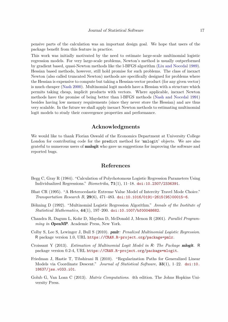
An important factor to consider in parallel speedups of the whole program is Amdahl’s lawwhich limits the maximum speedup that may be achieved by any parallel program (see Chap-ter 6 of Chandra, Dagum, Kohr, Maydan, McDonald, and Menon 2001). Assuming par-allelization between n threads, Amdahl’s law states that the ultimate speedup is given by:Sn = 1
fs+(1−fs)/n , where fs is the fraction of non-parallelized, serial code. Table 3 lists theobserved speedups on 2, 4 and 8 processor cores together with fs for problems of Table 1.We take the time not spent in computing the Hessian as the “serial time” to compute fs
and neglect the serial time spent in setting up the parallel computation in Hessian calcula-tion, which mainly involves spawning threads in OpenMP and allocating separate blocks ofworking memory for each thread. For type “Z” problems, this is an underestimate becausesome Hessian calculation is also serial. Our tests have shown that compared to the Hessian
16 mnlogit: Fast Estimation of Multinomial Logit Models in R
0 2 4 6 8 10 12 14 16procs
2
4
6
8
10
Spee
dup
X (np = 4950)
Y (np = 5000)
YZ (np = 4505)
Z (np = 50)
Linear Speedup
Figure 1: Parallel Hessian calculation speedup (ratio of parallel to single thread runningtime) for 2, 4, 8, 16, processor cores for problems of Table 1. The dashed “Linear Speedup”guideline represents perfect parallelization.
Problem Serial fraction (fs) S2 S4 S8
X 0.124 1.76 (1.78) 2.87 (2.92) 4.04 (4.28)Y 0.258 1.59 (1.62) 2.26 (2.27) 2.59 (2.85)Z 0.780 1.08 (1.12) 1.14 (1.20) 1.17 (1.24)
YZ 0.257 1.44 (1.59) 2.08 (2.26) 2.36 (2.86)
Table 3: Parallel speedup of mnlogit versus serial performance (parentheses: predictedultimate speedup from Amdahl’s law) for problems of Table 1. S2, S4 and S8 are observedspeedups on 2, 4 and 8 processor cores respectively, while fs is the estimated fraction of timespent in the serial portion of the code.
calculation, the (serial) work required in setting up parallel computation is negligible, exceptfor very small problems.
5. Discussion
Through mnlogit we seek to provide the community a package which combines quick calcula-tion and the ability to handle data collinearity with a software interface which encompassesa wide range of multinomial logit models and data types used in econometrics and machinelearning. Our main idea, exploiting matrix structure in large scale linear algebra calculationsis not novel; however this work is the first, as far as we are aware, to apply it to the estima-tion of multinomial logit models problems in a working software package. The parallelizationcapability of mnlogit, which can easily add a 2×–4× factor of speedup on now ubiquitousmulticore computers, is another angle which is underutilized in statistical software. Althoughmnlogit code is not parallelized to the maximum possible extent, parallelizing the most ex-
Journal of Statistical Software 17
pensive parts of the calculation was an important design goal. We hope that users of thepackage benefit from this feature in practice.
This work was initially motivated by the need to estimate large-scale multinomial logisticregression models. For very large-scale problems, Newton’s method is usually outperformedby gradient based, quasi-Newton methods like the l-BFGS algorithm (Liu and Nocedal 1989).Hessian based methods, however, still hold promise for such problems. The class of inexactNewton (also called truncated Newton) methods are specifically designed for problems wherethe Hessian is expensive to compute but taking a Hessian-vector product (for any given vector)is much cheaper (Nash 2000). Multinomial logit models have a Hessian with a structure whichpermits taking cheap, implicit products with vectors. Where applicable, inexact Newtonmethods have the promise of being better than l-BFGS methods (Nash and Nocedal 1991)besides having low memory requirements (since they never store the Hessian) and are thusvery scalable. In the future we shall apply inexact Newton methods to estimating multinomiallogit models to study their convergence properties and performance.
Acknowledgments
We would like to thank Florian Oswald of the Economics Department at University CollegeLondon for contributing code for the predict method for ‘mnlogit’ objects. We are alsograteful to numerous users of mnlogit who gave us suggestions for improving the software andreported bugs.
References
Begg C, Gray R (1984). “Calculation of Polychotomous Logistic Regression Parameters UsingIndividualized Regressions.” Biometrika, 71(1), 11–18. doi:10.2307/2336391.
Bhat CR (1995). “A Heterocedastic Extreme Value Model of Intercity Travel Mode Choice.”Transportation Research B, 29(6), 471–483. doi:10.1016/0191-2615(95)00015-6.
Böhning D (1992). “Multinomial Logistic Regression Algorithm.” Annals of the Institute ofStatistical Mathematics, 44(1), 197–200. doi:10.1007/bf00048682.
Chandra R, Dagum L, Kohr D, Maydan D, McDonald J, Menon R (2001). Parallel Program-ming in OpenMP. Academic Press, New York.
Colby S, Lee S, Lewinger J, Bull S (2010). pmlr: Penalized Multinomial Logistic Regression.R package version 1.0, URL https://CRAN.R-project.org/package=pmlr.
Croissant Y (2013). Estimation of Multinomial Logit Model in R: The Package mlogit. R
package version 0.2-4, URL https://CRAN.R-project.org/package=mlogit.
Friedman J, Hastie T, Tibshirani R (2010). “Regularization Paths for Generalized LinearModels via Coordinate Descent.” Journal of Statistical Software, 33(1), 1–22. doi:10.
18637/jss.v033.i01.
Golub G, Van Loan C (2013). Matrix Computations. 4th edition. The Johns Hopkins Uni-versity Press.
18 mnlogit: Fast Estimation of Multinomial Logit Models in R
Hasan A, Zhiyu W, Mahani AS (2015). mnlogit: Multinomial Logit Model. R package version1.2.4, URL https://CRAN.R-project.org/package=mnlogit.
Hastie T, Tibshirani R, Friedman J (2009). The Elements of Statistical Learning: DataMining, Inference and Prediction. 2nd edition. Springer-Verlag.
Jurka T (2012). “maxent: An R Package for Low-Memory Multinomial Logistic Regressionwith Support for Semi-Automated Text Classification.” The R Journal, 4(1), 56–59. URLhttps://journal.R-project.org/archive/2012-1/RJournal_2012-1_Jurka.pdf.
Komarek P, Moore A (2005). “Making Logistic Regression a Core Data Mining Tool: APractical Investigation of Accuracy, Speed, and Simplicity.” Technical report, CarnegieMellon University.
Li J (2013). “Logistic Regression.” Course Notes. URL http://sites.stat.psu.edu/
~jiali/course/stat597e/notes2/logit.pdf.
Lin CJ, Weng R, Keerthi S (2008). “Trust Region Newton Method for Large-Scale LogisticRegression.” Journal of Machine Learning Research, 9, 627–650.
Liu D, Nocedal J (1989). “On the Limited Memory BFGS Method for Large Scale Optimiza-tion.” Mathematical Programming, 45(1), 503–528. doi:10.1007/bf01589116.
McFadden D (1974). “The Measurement of Urban Travel Demand.” Journal of Public Eco-nomics, 3(4), 303–328. doi:10.1016/0047-2727(74)90003-6.
Nash S (2000). “A Survey of Truncated-Newton Methods.” Journal of Computational andApplied Mathematics, 124(1–2), 45–59. doi:10.1016/s0377-0427(00)00426-x.
Nash S, Nocedal J (1991). “A Numerical Study of the Limited Memory BFSG Method and theTruncated-Newton Method for Large-Scale Optimization.” SIAM Journal of Optimization,1(3), 358–372. doi:10.1137/0801023.
Nigam K, Lafferty J, McCallum A (1999). “Using Maximum Entropy for Text Classification.”In IJCAI’99 Workshop on Machine Learning for Information Filtering.
Nocedal J (1990). “The Performance of Several Algorithms for Large Scale UnconstrainedOptimization.” In Large Scale Numerical Optimization, pp. 138–151. SIAM.
Nocedal J (1992). “Theory of Algorithms for Unconstrained Optimization.” Acta Numerica,1, 199–242. doi:10.1017/s0962492900002270.
Nocedal J, Wright S (2000). Numerical Optmization. 2nd edition. Springer-Verlag.
OpenMP Architecture Review Board (2015). OpenMP Application Program Interface. Ver-sion 4.5, URL http://www.openmp.org/.
R Core Team (2016). R: A Language and Environment for Statistical Computing. R Founda-tion for Statistical Computing, Vienna, Austria. URL https://www.R-project.org/.
Sevcikova H, Raftery A (2013). mlogitBMA: Bayesian Model Averaging for Multinomial LogitModel. R package version 0.1-6, URL https://CRAN.R-project.org/package=mlogitBMA.
Journal of Statistical Software 19
Train K (2003). Discrete Choice Methods with Simulation. Cambridge University Press,Cambridge.
Trefethen L, Bau D (1997). Numerical Linear Algebra. SIAM, Philadelphia.
Venables W, Ripley B (2002). Modern Applied Statistics with S. 4th edition. Springer-Verlag,New York. URL http://www.stats.ox.ac.uk/pub/MASS4/.
Yee T (2010). “The VGAM Package for Categorical Data Analysis.” Journal of StatisticalSoftware, 32(10), 1–34. doi:10.18637/jss.v032.i10.
Zeileis A, Croissant Y (2010). “Extended Model Formulas in R: Multiple Parts and MultipleResponses.” Journal of Statistical Software, 34(1), 1–13. doi:10.18637/jss.v034.i01.
Zeileis A, Hothorn T (2002). “Diagnostic Checking in Regression Relationships.” R News,2(3), 7–10. URL https://CRAN.R-project.org/doc/Rnews/.
20 mnlogit: Fast Estimation of Multinomial Logit Models in R
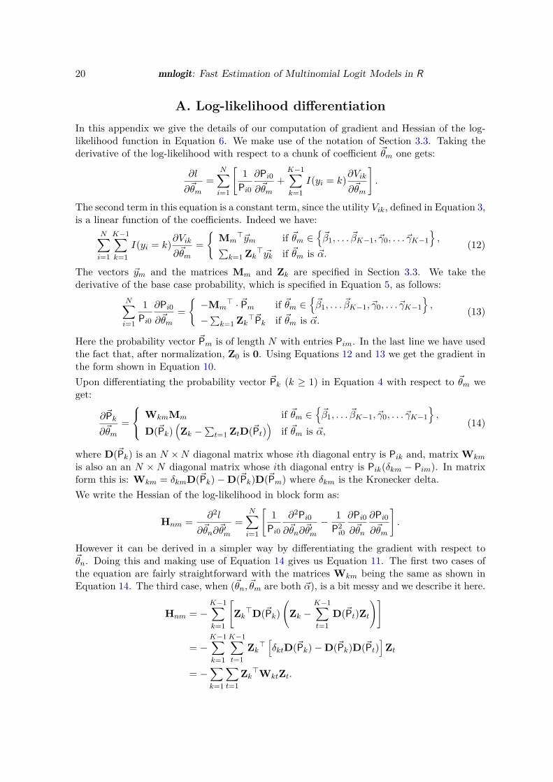
A. Log-likelihood differentiation
In this appendix we give the details of our computation of gradient and Hessian of the log-likelihood function in Equation 6. We make use of the notation of Section 3.3. Taking thederivative of the log-likelihood with respect to a chunk of coefficient ~θm one gets:
∂l
∂~θm
=N∑
i=1
[
1
Pi0
∂Pi0
∂~θm
+K−1∑
k=1
I(yi = k)∂Vik
∂~θm
]
.
The second term in this equation is a constant term, since the utility Vik, defined in Equation 3,is a linear function of the coefficients. Indeed we have:
N∑
i=1
K−1∑
k=1
I(yi = k)∂Vik
∂~θm
=
{
Mm⊤~ym if ~θm ∈
{
~β1, . . . ~βK−1, ~γ0, . . . ~γK−1
}
,∑
k=1 Zk⊤ ~yk if ~θm is ~α.
(12)
The vectors ~ym and the matrices Mm and Zk are specified in Section 3.3. We take thederivative of the base case probability, which is specified in Equation 5, as follows:
N∑
i=1
1
Pi0
∂Pi0
∂~θm
=
{
−Mm⊤ · ~Pm if ~θm ∈
{
~β1, . . . ~βK−1, ~γ0, . . . ~γK−1
}
,
−∑
k=1 Zk⊤~Pk if ~θm is ~α.
(13)
Here the probability vector ~Pm is of length N with entries Pim. In the last line we have usedthe fact that, after normalization, Z0 is 0. Using Equations 12 and 13 we get the gradient inthe form shown in Equation 10.
Upon differentiating the probability vector ~Pk (k ≥ 1) in Equation 4 with respect to ~θm weget:
∂~Pk
∂~θm
=
WkmMm if ~θm ∈{
~β1, . . . ~βK−1, ~γ0, . . . ~γK−1
}
,
D(~Pk)(
Zk −∑
t=1 ZtD(~Pt))
if ~θm is ~α,(14)
where D(~Pk) is an N × N diagonal matrix whose ith diagonal entry is Pik and, matrix Wkm
is also an an N × N diagonal matrix whose ith diagonal entry is Pik(δkm − Pim). In matrixform this is: Wkm = δkmD(~Pk) − D(~Pk)D(~Pm) where δkm is the Kronecker delta.
We write the Hessian of the log-likelihood in block form as:
Hnm =∂2l
∂~θn∂~θ′m
=N∑
i=1
[
1
Pi0
∂2Pi0
∂~θn∂~θ′m
−1
P2i0
∂Pi0
∂~θn
∂Pi0
∂~θm
]
.
However it can be derived in a simpler way by differentiating the gradient with respect to~θn. Doing this and making use of Equation 14 gives us Equation 11. The first two cases ofthe equation are fairly straightforward with the matrices Wkm being the same as shown inEquation 14. The third case, when (~θn, ~θm are both ~α), is a bit messy and we describe it here.
Hnm = −K−1∑
k=1
[
Zk⊤D(~Pk)
(
Zk −K−1∑
t=1
D(~Pt)Zt
)]
= −K−1∑
k=1
K−1∑
t=1
Zk⊤[
δktD(~Pk) − D(~Pk)D(~Pt)]
Zt
= −∑
k=1
∑
t=1
Zk⊤WktZt.
Journal of Statistical Software 21
Here the last line follows from the definition of matrix Wkt as used in Equation 14.
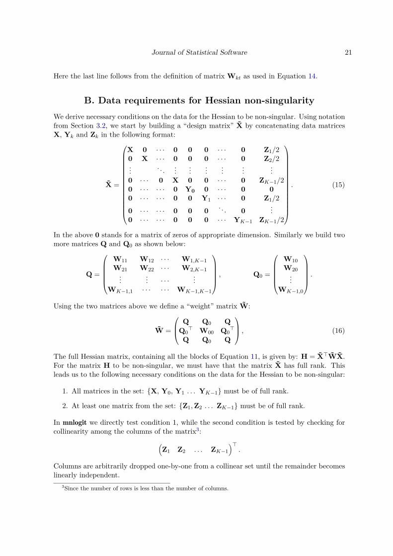
B. Data requirements for Hessian non-singularity
We derive necessary conditions on the data for the Hessian to be non-singular. Using notationfrom Section 3.2, we start by building a “design matrix” X̃ by concatenating data matricesX, Yk and Zk in the following format:
X̃ =
X 0 · · · 0 0 0 · · · 0 Z1/20 X · · · 0 0 0 · · · 0 Z2/2...
. . ....
......
......
...0 · · · 0 X 0 0 · · · 0 ZK−1/20 · · · · · · 0 Y0 0 · · · 0 0
0 · · · · · · 0 0 Y1 · · · 0 Z1/2
0 · · · · · · 0 0 0. . . 0
...0 · · · · · · 0 0 0 · · · YK−1 ZK−1/2
. (15)
In the above 0 stands for a matrix of zeros of appropriate dimension. Similarly we build twomore matrices Q and Q0 as shown below:
Q =
W11 W12 · · · W1,K−1
W21 W22 · · · W2,K−1...
... · · ·...
WK−1,1 · · · · · · WK−1,K−1
, Q0 =
W10
W20...
WK−1,0
.
Using the two matrices above we define a “weight” matrix W̃:
W̃ =
Q Q0 Q
Q0⊤ W00 Q0
⊤
Q Q0 Q
, (16)
The full Hessian matrix, containing all the blocks of Equation 11, is given by: H = X̃⊤W̃X̃.For the matrix H to be non-singular, we must have that the matrix X̃ has full rank. Thisleads us to the following necessary conditions on the data for the Hessian to be non-singular:
1. All matrices in the set: {X, Y0, Y1 . . . YK−1} must be of full rank.
2. At least one matrix from the set: {Z1, Z2 . . . ZK−1} must be of full rank.
In mnlogit we directly test condition 1, while the second condition is tested by checking forcollinearity among the columns of the matrix3:
(
Z1 Z2 . . . ZK−1
)⊤
.
Columns are arbitrarily dropped one-by-one from a collinear set until the remainder becomeslinearly independent.
3Since the number of rows is less than the number of columns.
22 mnlogit: Fast Estimation of Multinomial Logit Models in R
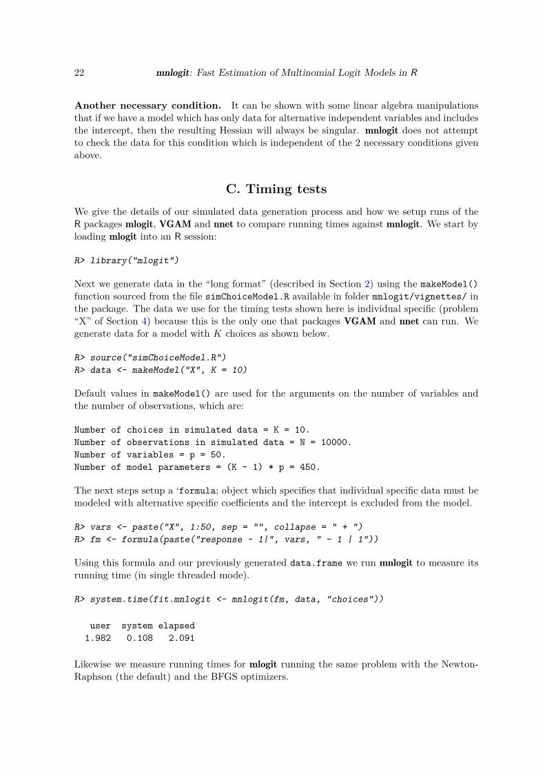
Another necessary condition. It can be shown with some linear algebra manipulationsthat if we have a model which has only data for alternative independent variables and includesthe intercept, then the resulting Hessian will always be singular. mnlogit does not attemptto check the data for this condition which is independent of the 2 necessary conditions givenabove.
C. Timing tests
We give the details of our simulated data generation process and how we setup runs of theR packages mlogit, VGAM and nnet to compare running times against mnlogit. We start byloading mlogit into an R session:
R> library("mlogit")
Next we generate data in the “long format” (described in Section 2) using the makeModel()
function sourced from the file simChoiceModel.R available in folder mnlogit/vignettes/ inthe package. The data we use for the timing tests shown here is individual specific (problem“X” of Section 4) because this is the only one that packages VGAM and nnet can run. Wegenerate data for a model with K choices as shown below.
R> source("simChoiceModel.R")
R> data <- makeModel("X", K = 10)
Default values in makeModel() are used for the arguments on the number of variables andthe number of observations, which are:
Number of choices in simulated data = K = 10.
Number of observations in simulated data = N = 10000.
Number of variables = p = 50.
Number of model parameters = (K - 1) * p = 450.
The next steps setup a ‘formula; object which specifies that individual specific data must bemodeled with alternative specific coefficients and the intercept is excluded from the model.
R> vars <- paste("X", 1:50, sep = "", collapse = " + ")
R> fm <- formula(paste("response ~ 1|", vars, " - 1 | 1"))
Using this formula and our previously generated data.frame we run mnlogit to measure itsrunning time (in single threaded mode).
R> system.time(fit.mnlogit <- mnlogit(fm, data, "choices"))
user system elapsed
1.982 0.108 2.091
Likewise we measure running times for mlogit running the same problem with the Newton-Raphson (the default) and the BFGS optimizers.
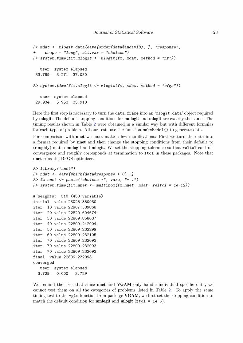
Journal of Statistical Software 23
R> mdat <- mlogit.data(data[order(data$indivID), ], "response",
+ shape = "long", alt.var = "choices")
R> system.time(fit.mlogit <- mlogit(fm, mdat, method = "nr"))
user system elapsed
33.789 3.271 37.080
R> system.time(fit.mlogit <- mlogit(fm, mdat, method = "bfgs"))
user system elapsed
29.934 5.953 35.910
Here the first step is necessary to turn the data.frame into an ‘mlogit.data’ object requiredby mlogit. The default stopping conditions for mnlogit and mlogit are exactly the same. Thetiming results shown in Table 2 were obtained in a similar way but with different formulasfor each type of problem. All our tests use the function makeModel() to generate data.
For comparison with nnet we must make a few modifications: First we turn the data intoa format required by nnet and then change the stopping conditions from their default to(roughly) match mnlogit and mlogit. We set the stopping tolerance so that reltol controlsconvergence and roughly corresponds at termination to ftol in these packages. Note thatnnet runs the BFGS optimizer.
R> library("nnet")
R> ndat <- data[which(data$response > 0), ]
R> fm.nnet <- paste("choices ~", vars, "- 1")
R> system.time(fit.nnet <- multinom(fm.nnet, ndat, reltol = 1e-12))
# weights: 510 (450 variable)
initial value 23025.850930
iter 10 value 22907.389868
iter 20 value 22820.604674
iter 30 value 22809.858037
iter 40 value 22809.242004
iter 50 value 22809.232299
iter 60 value 22809.232105
iter 70 value 22809.232093
iter 70 value 22809.232093
iter 70 value 22809.232093
final value 22809.232093
converged
user system elapsed
3.729 0.000 3.729
We remind the user that since nnet and VGAM only handle individual specific data, wecannot test them on all the categories of problems listed in Table 2. To apply the sametiming test to the vglm function from package VGAM, we first set the stopping condition tomatch the default condition for mnlogit and mlogit (ftol = 1e-6).
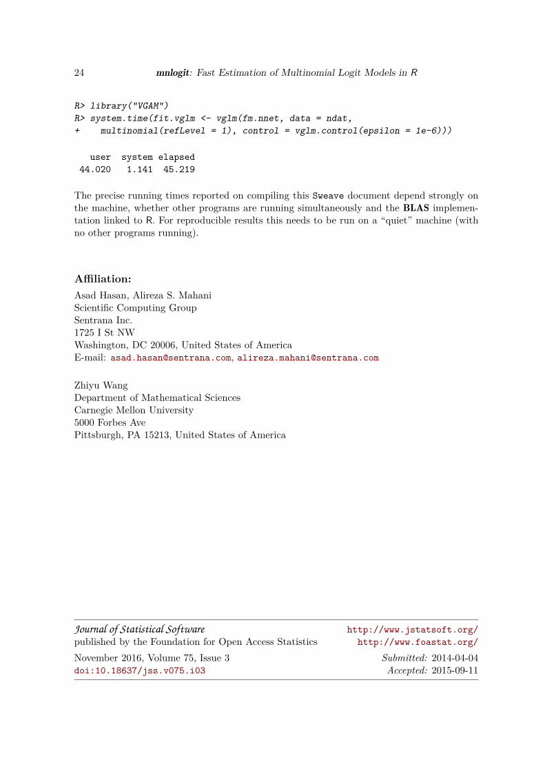
24 mnlogit: Fast Estimation of Multinomial Logit Models in R
R> library("VGAM")
R> system.time(fit.vglm <- vglm(fm.nnet, data = ndat,
+ multinomial(refLevel = 1), control = vglm.control(epsilon = 1e-6)))
user system elapsed
44.020 1.141 45.219
The precise running times reported on compiling this Sweave document depend strongly onthe machine, whether other programs are running simultaneously and the BLAS implemen-tation linked to R. For reproducible results this needs to be run on a “quiet” machine (withno other programs running).
Affiliation:
Asad Hasan, Alireza S. MahaniScientific Computing GroupSentrana Inc.1725 I St NWWashington, DC 20006, United States of AmericaE-mail: [email protected], [email protected]
Zhiyu WangDepartment of Mathematical SciencesCarnegie Mellon University5000 Forbes AvePittsburgh, PA 15213, United States of America
Journal of Statistical Software http://www.jstatsoft.org/
published by the Foundation for Open Access Statistics http://www.foastat.org/
November 2016, Volume 75, Issue 3 Submitted: 2014-04-04doi:10.18637/jss.v075.i03 Accepted: 2015-09-11