essays on wage determination factors and...
TRANSCRIPT

Hitotsubashi University Repository
TitleEssays on Wage Determination Factors and Individual
Heterogeneity : Evidence from Japanese Panel Data
Author(s) SUN, Yawen
Citation
Issue Date 2016-03-18
Type Thesis or Dissertation
Text Version ETD
URL http://doi.org/10.15057/27894
Right

Essays on Wage Determination Factors andIndividual Heterogeneity
—Evidence from Japanese Panel Data—
Yawen Sun
Graduate School of EconomicsHitotsubashi University
2016

AcknowledgementOver the past four years I have received support and encouragement from a
great number of individuals. I would like to express my sincere gratitude to myadvisor Professor Daiji Kawaguchi for the continuous support of my Ph.D studyand related research, for his patience, motivation, and immense knowledge. Hisguidance helped me in all the time of research and writing of this dissertation.I also wish to thank Professor Takashi Oshio, for his insightful comments andencouragement. Without their continuing support and encouragement, I wouldnever have completed this dissertation. In addition, advice and comments givenby Professor Ryo Kambayashi, Associate Professor Yuko Ueno and AssociateProfessor Emiko Usui has been a great help in improving this dissertation. I wouldalso like to thank the teachers who give practical comments at conferences.
I thank Panel Data Research Center at Keio University, Institute of Socialand Economic Research at Osaka University and Professor Toshiaki Tachibanakifor permission to use their panel data to conduct my research and complete thisdissertation.
Special thanks to my fellow mates and dormitory mates for the stimulatingdiscussions, and for all the fun we have had in the last four years. Finally, I amdeeply greatful to my family for their enduring emotional and financial support.

Contents1 Chapter 1 Introduction 1
1.1 Overview . . . . . . . . . . . . . . . . . . . . . . . . . . . . . . 11.2 Summary of Chapters . . . . . . . . . . . . . . . . . . . . . . . . 3
2 Chapter 2 Smoking and Wage Rates 92.1 Introduction . . . . . . . . . . . . . . . . . . . . . . . . . . . . . 92.2 Literature Review . . . . . . . . . . . . . . . . . . . . . . . . . . 112.3 Data and Descriptive Statistics . . . . . . . . . . . . . . . . . . . 14
2.3.1 Data . . . . . . . . . . . . . . . . . . . . . . . . . . . . . 142.3.2 Descriptive Statistics . . . . . . . . . . . . . . . . . . . . 16
2.4 Smoking and Wage Rate . . . . . . . . . . . . . . . . . . . . . . 222.4.1 Empirical Methodology . . . . . . . . . . . . . . . . . . 222.4.2 Problem and Solution . . . . . . . . . . . . . . . . . . . . 222.4.3 Empirical Results and Discussion . . . . . . . . . . . . . 242.4.4 Instrumental Variable Estimation . . . . . . . . . . . . . . 30
2.5 Robustness Check . . . . . . . . . . . . . . . . . . . . . . . . . . 342.5.1 Company Size and Job Status . . . . . . . . . . . . . . . 342.5.2 Regular Workers and Non-regular Workers . . . . . . . . 372.5.3 Additional Estimations . . . . . . . . . . . . . . . . . . . 40
2.6 Discussion . . . . . . . . . . . . . . . . . . . . . . . . . . . . . . 422.6.1 Alcohol Consumption . . . . . . . . . . . . . . . . . . . 422.6.2 Exercise . . . . . . . . . . . . . . . . . . . . . . . . . . . 45
2.7 Conclusion . . . . . . . . . . . . . . . . . . . . . . . . . . . . . 48
3 Chapter 3 Men’s Wages and Intra-household Specialization 533.1 Introduction . . . . . . . . . . . . . . . . . . . . . . . . . . . . . 533.2 Data and Descriptive Statistics . . . . . . . . . . . . . . . . . . . 60
3.2.1 Data . . . . . . . . . . . . . . . . . . . . . . . . . . . . . 603.2.2 Descriptive Statistics . . . . . . . . . . . . . . . . . . . . 61
3.3 Intra-household Specialization and Wage Premium . . . . . . . . 683.3.1 Empirical Methodology . . . . . . . . . . . . . . . . . . 683.3.2 Empirical Results and Discussion . . . . . . . . . . . . . 72
3.4 Robustness Check . . . . . . . . . . . . . . . . . . . . . . . . . . 763.4.1 Subsample Analysis . . . . . . . . . . . . . . . . . . . . 763.4.2 First Difference Estimation and “Past” Wife’s Working
Status . . . . . . . . . . . . . . . . . . . . . . . . . . . . 78
i

3.4.3 Hours Spent on Housework Among Couples . . . . . . . 813.4.4 Company Size . . . . . . . . . . . . . . . . . . . . . . . 843.4.5 Age Groups . . . . . . . . . . . . . . . . . . . . . . . . . 89
3.5 Conclusion . . . . . . . . . . . . . . . . . . . . . . . . . . . . . 90
4 Chapter 4 Variation in the Effects of the Big-Five Personality Traits;The 10-Item Scale versus the 44-Item Scale 954.1 Introduction . . . . . . . . . . . . . . . . . . . . . . . . . . . . . 954.2 Literature Review . . . . . . . . . . . . . . . . . . . . . . . . . . 974.3 Data and Descriptive Statistics . . . . . . . . . . . . . . . . . . . 100
4.3.1 4.3.1 Data . . . . . . . . . . . . . . . . . . . . . . . . . . 1004.3.2 Descriptive Statistics and Weighting . . . . . . . . . . . . 101
4.3.2.1 Descriptive Statistics . . . . . . . . . . . . . . 1014.3.2.2 Descriptive Statistics with Inverse Probability
Weighting . . . . . . . . . . . . . . . . . . . . 1034.4 Results and Discussion . . . . . . . . . . . . . . . . . . . . . . . 106
4.4.1 Correlations between the Big-Five personality traits andIndividual Attributes . . . . . . . . . . . . . . . . . . . . 106
4.4.2 Effect of the Big-Five personality traits on Annual Income 1134.4.3 Item Effects . . . . . . . . . . . . . . . . . . . . . . . . . 1164.4.4 Principal Component Analysis . . . . . . . . . . . . . . . 124
4.5 Conclusion . . . . . . . . . . . . . . . . . . . . . . . . . . . . . 127
5 Chapter 5 Conclusion 131
A Appendix Tables 133
ii

1 Chapter 1 Introduction
1.1 Overview
Verifying factors influencing wage level and changes has remained a key issue
in labor economics. Since the Mincer (1974) earnings function based on human
capital theory, many empirical studies have shown that years of schooling and
labor market experience are major factors affecting wage determination in the
United States and many other countries (Borjas 2012; Burusku 2006; Willis 1987).
Several studies analyzing the effects of returns of education, work experience,
and job tenure on wages use the Mincer equation to address the issues of omitted
variables and biased estimate heterogeneity (Altonji and Shakotko 1987; Abraham
and Farber 1987; Marshall and Zarkin 1987). In the case of Japan, Tachibanaki
and Taki (1990) pointed out that the problem of omitted variables or heterogene-
ity does not apply to tenure because Japan has almost no labor turnover; however,
this trend has changed over the years. According to a 2013 labor analysis report
by the Ministry of Health, Labour and Welfare, the labor turnover rate is increas-
ing on an annual basis, especially among the younger age groups (20s and 30s).
Over the years, people’s way of working has changed especially after the collapse
of the Japanese permanent employment system. This points to the need to ad-
dress the problem of omitted variables and heterogeneity when discussing wage
determination in Japan.
Many studies on wage determination use cross-sectional data, although this
1

creates a potential heterogeneity problem. This thesis investigates factors affect-
ing wages using Japanese panel data. According to Hsiao (2003) and Baltagi
(2013), panel data can eliminate potential sources of time-invariant unobservable
individual heterogeneity, which cannot be controlled for using time-series and
cross-sectional data.
There are several factors influencing wages, including family and social en-
vironment and habituation. Economists have investigated the influences of be-
havioral factors on economic decision-making. In this thesis, we investigate the
effects of two behavioral factors, smoking and marriage, on wages. In addition,
we use two methods to measure the Big Five personality traits as potential un-
observable individual heterogeneity to discuss the validity of unstable variables
in economic empirical analyses. Recent studies, particularly in the field of eco-
nomic behavior, use unstable variables such as time discount rate, risk aversion
rate, locus of control, and other personality traits as proxy variables for individual
unobservable heterogeneity.
The results revealed that individual unobservable heterogeneity affects wage
determination through two behavioral factors, smoking and intra-household spe-
cialization. In addition, it is important to carefully interpret estimation results
when using unstable variables such as the Big-Five personality traits as a proxy
variable of individual unobservable heterogeneity.
2

1.2 Summary of Chapters
In Chapters 2 and 3, we use Japanese panel data to verify factors contributing
the wage disparity between smokers and nonsmokers and between males who
have full-time housewives and those are single or whose wives also have full-time
or part-time jobs (hereinafter other males).
Specifically, in Chapter 2, we present our research of smoking behavior. As
is widely known, smoking is known to have negative effects on health, and to
discourage the practice, governments frequently implement policies such as tax
increases or restrictions on public smoking. To evaluate these policies, it is neces-
sary to grasp a clearer understanding of the economic benefits and costs of reduc-
ing the number of smokers. By conducting panel data analysis while controlling
for unobserved heterogeneity, Chapter 2 shows that smoking is not the main factor
causing observed wage differentials between smokers and nonsmokers in Japan.
As for the relationship between smoking and wages, we find that male smokers
receive lower hourly wages than male nonsmokers. Smoking behavior generally
depends on environmental, congenital, or social factors. These factors, however,
do not only affect smoking behavior but also the wages of these individuals. To
isolate the effect of smoking on wages, we control for individual heterogeneity
using panel data to verify the existence of such an effect.
Using tax change as an instrumental variable in the fixed effects model and
several robustness checks, the results show that smoking has no statistically sig-
nificant effect on wage rate. This suggests that smoking does not directly affect
3

wages; rather, unobserved individual heterogeneity (other factors influencing both
smoking and wages) leads to wage differences between smokers and nonsmokers.
Nevertheless, smoking can affect wages in the long run through health problems.
The nine-year panel data used in this research, however, is insufficient to capture
the long-term indirect health effects. Thus, future research should consider ana-
lyzing indirect health effects using panel data spread across a wider time frame.
In Chapter 3, we attempt to answer the research question “Do wedding bells
bring wealth?” In Japan, it is commonly believed that marriage can increase men’s
income level and a cursory view of the data suggests that this may hold true, par-
ticularly if the man’s spouse is a full-time housewife. Further, Becker (1991)
argues that women hold a comparative advantage over men in housework; thus,
focusing on their jobs after marriage can result in a male wage premium. Us-
ing Japanese panel data, this chapter investigates the relationship between marital
status and wage rate for men and finds that when unobserved heterogeneity is
properly controlled for, marital status and intra-household specialization have no
effect on men’s wage. To isolate the effect of intra-household specialization, we
use the interaction terms of marital status and wife’s working status as dummy
variables. While the results for the ordinary least squares estimation show that a
man who has a full-time housewife earns higher wages than other males, the fixed
effects model finds no such effect.
Thus, this research suggests that it is not a wife’s work status but unobservable
individual heterogeneity that causes wage differentials between men with a spouse
who is a full-time housewife and other males. In other words, there are various
4

unobserved characteristics that can influence both marital status and higher wages
for men, for example, competence and attractiveness are values and appreciated
by both a boss and a potential spouse. Interestingly, a wife’s working status does
not depend on the man’s wage rate. Thus, future work should attempt to clarify
the factors of unobservable individual heterogeneity that affect men’s wages and
the relationship between marriage and wage rate for women.
In Chapters 2 and 3, we find that wage differences between smokers and non-
smokers and between married males who have full-time housewives and other
males can be ascribed to individual unobservable differences, even after control-
ling for years of schooling, work experience and job tenure effects.
Chapter 4 focuses on the Big Five personality traits―Extraversion, Agreeable-
ness, Conscientiousness, Neuroticism, and Openness to experience―to test the
validity of unstable factors when using proxy variables of individual unobserv-
able heterogeneity in economic empirical analyses; this is an established method
to measure personality in the field of psychology.
We use two datasets that include 10-item and 44-item inventories to measure
the Big-Five personality traits. In general, the procedure to measure personality
includes the 44-item questionnaire, which is time consuming yet commonly used
in psychology studies, while the 10-item questionnaire has been recently devel-
oped and saves time for researchers and respondents. Both procedures are certified
as sufficient to measure personality traits in psychology analyses. However, this
does not mean that both approaches provide similar results in economic analyses.
In Chapter 4, we estimate the Mincer equation with personality traits to compare
5

the effect of personality on wages between the Big-Five variables estimated using
10 and from 44-item questionnaires. The results show that Agreeableness dif-
fer between both questionnaire types. To evaluate the factors underpinning these
differences, we estimate the effect of each item on the outcome variables. We
use the first principle component obtained by conducting the principle compo-
nent analysis, instead of the Big-Five scores derived by adding up the scores for
each item, to evaluate the appropriateness of weight given to each item’s response.
However, the results still show differences for Agreeableness between the 10 and
44-item questionnaires, suggesting that the differences are generated from those
in the expressions of each item between the two questionnaires. In this case, if
questionnaires demonstrate different nuances, then the personality traits estimated
using them may capture varying personality traits. The main implication of this
finding is that short questions save time for respondents and researchers and have
a consistent effect on economic outcomes in comparison to widely used and time-
consuming questions; however, this is applicable to “some’ personality traits, not
all. When using short questions in economic empirical researches, it is impor-
tant to pay careful attention to the expression of each item in the questionnaire,
particularly those based on Agreeableness.
In sum, we evaluated two behavioral factors that may affect wage determina-
tion and found that wage differences appeared owing to individual unobservable
heterogeneity, even if we control for years of schooling or work experience. Next,
we attempt to check the validity of the unstable variables, or the Big Five person-
ality traits used as proxy variables of unobservable individual heterogeneity. Our
6

results highlight the need to exercise precaution when interpreting estimates for
personality traits, which also depends on the type of questionnaire used.
We recommend further research on the mechanisms underlying the relation-
ship between wages and smoking, marital status, and individual unobservable het-
erogeneity. In addition, it is necessary to have long-term panel data to verify the
factors affecting wage determination in Japan.
The remainder of this thesis is organized as follows. Chapter 2 summarizes
the analysis of the effects of smoking on wage determination. Chapter 3 dis-
cusses the relationship between intra-household specialization and wages. Chap-
ter 4 presents the analysis of the Big-Five personality traits. Chapter 5 offers
concluding remarks.
7

References[1] Abraham, K.G. and H.S. Farber (1987) “Job Duration, Sniority, and Earn-
ings.” American Economic Review. 77, 278- 297.
[2] Altonji, J.G. and R.A. Shakotko (1987) “Do Wages Rise with Job Senior-ity?.” Review of Economic Studies. 54, 437- 459.
[3] Baltagi, B. H. (2013) Econometric Analysis of Panel Data. fifth Edition.Wiley Press.
[4] Becker, G. S. (1991) A Treatise on the Family. Cambridge. MA: HarvardUniversity Press.
[5] Borjas, G.J. (2012) Labor Economics. sixth Edition. McGraw-Hill Educa-tion Press.
[6] Burusku, B. (2006) “Training and Lifetime Income.” American EconomicReview. 96, 832- 46.
[7] Hsiao, C. (2003) Analysis of Panel Data. second Edition. Cambridge Uni-versity Press.
[8] Marshall, R.C. and G.A. Zarkin (1987) “The Effect of Job Tenure on WageOffers.” Journal of Labor Economics. 5, 301- 324.
[9] Mincer, J. (1974), Schooling, Experience and Earnings. NBER andColumbia Press.
[10] Tachibanaki, T. and A. Taki (1990) “Wage Determination in Japan: A The-oretical and Empirical Investigation.” H. Konig (Eds.) Economics of WageDetermination. 39- 64, Springer-Verlag Press.
[11] The Ministry of Health, Labour and Welfare (2013). “Heisei 25Nen Ban Rodo Keizai no Bunseki” (The 2013th Analysis of LaborEconomy). The Ministry of Health, Labour and Welfare webpage).http://www.mhlw.go.jp/wp/hakusyo/roudou/13/13-1.html (accessed Novem-ber 12, 2015).
[12] Willis, R. (1987) “Wage Determinants: A Survey and Reinterpretation ofHuman Capital Earnings Functions.” O. Ashenfelter and R. Layard (Eds.)Handbook of Labor Economics. 1, 525- 602.
8

2 Chapter 2 Smoking and Wage Rates
2.1 Introduction
This chapter aims to verify the effect of smoking on hourly wages using Japanese
panel data to determine whether encouraging people to quit smoking is an effec-
tive way to increase productivity. As we can find wage disparities between smok-
ers and nonsmokers, there are many economic studies into the effects of smoking
on labor outcomes from the 1990s. This chapter mainly focuses on the effect of
smoking on wages in Japan to evaluate causes behind wage disparities between
smokers and nonsmokers, and discuss the relationship between quitting smoking
and productivity.
Smoking not only directly affects health, but also leads to some economic
costs. Since the 1960s, there have been many studies into the effects of smoking
on health, demonstrating its negative effects.1 In addition to being a major cause of
rising healthcare costs, it also degrades labor productivity through its negative ef-
fect on workers’ health, for example, through absenteeism and lost future incomes
from health-related early retirement.2 Furthermore, decreasing levels of nicotine
in the blood lowers smokers’ concentration, leading them to increase their smok-
ing during working hours to compensate. Nicotine is also highly addictive, thus
extending its negative impact on smokers’ health.
1 Smoking is a major cause of lung cancer, cardiac arrests, brain deficiencies, and stroke (Hack-shaw, Law and Wald 1997; Benowitz 2008; Barik and Wonnacott 2009; Benowitz 2010).
2 For example, Ault et al. (1991). The World Bank (1999) noted other costs such as depressedenjoyment and difficulty in quitting smoking.
9

As knowledge of the negative effects of smoking are widely known, govern-
ments have implemented policies to reduce the economic costs of smoking, such
as increasing taxes on cigarettes, confining smokers to smoking areas expected to
encourage smokers to quit, and preventing nonsmokers from secondhand smoke
exposure.3 It is therefore necessary to estimate the economic cost of smoking
and the economic benefits of reduced smoking using a cost-benefit analysis of
smoking (The World Bank 1999: Chapter 6).
According to previous studies, there are two themes (smoking and absent
days, smoking and wage levels) in cost-benefit evaluations of smoking. In this
chapter, we focus on smoking and wage levels to verify the effect of smoking on
average hourly wages. Research into this topic in the 1990s showed that smok-
ers have statistically significant lower wage levels than nonsmokers (Levin et al.
1997), whereas research in the 2000s showed no wage differences between smok-
ers and nonsmokers (Lye and Hirschberg 2004; Yuda 2011). In this study, we
used Japanese panel data to control for considerable individual time-invariant en-
dogeneity to evaluate causes behind wage differences between smokers and non-
smokers. Additionally, we estimated the fixed effect instrumental (FE-IV) esti-
mation to control for individual time-variant endogeneity using the tax increases
on cigarettes. Furthermore, we checked the robustness of the results with some
additional analysis.
Our results indicate that no smoking effect on hourly wages exists for both
3 For example, the national tobacco tax, the cigarette special tax, the municipal tobacco tax,and the no street smoking ordinance.
10

men and women. Males have a statistically significant 9.4% wage difference be-
tween smokers and nonsmokers in the ordinary least squares (OLS) model, but it
disappears in the fixed effect (FE) model. This result indicates that wages do not
change when men quit smoking. Females have no statistically significant results
both in the OLS and FE models. If FE estimates are the result of the smoking
effect on wages, we believe that there are no statistically significant smoking ef-
fect on wages, and that wage differences among smokers and nonsmokers come
from other factors aside from smoking. FE-IV estimates also show the same re-
sults as in OLS and FE estimates. In some additional estimates: the model adding
occupation information, firm size, and employment status show similar results
providing robustness to the OLS and FE estimates. To consider estimation bias in
OLS estimates, we confirm that males have a lower bias and females have upper
bias.
The remainder of this chapter is organized as follows. Section 2.2 summarizes
the literature, Section 2.3 introduces the data and presents descriptive statistics,
Section 2.4 explains the method and discusses the main results, and Section 2.5
shows the results of the robustness check. Section 2.6 concludes.
2.2 Literature Review
There has been considerable research into workers and smoking around the
US and Europe. Those studies are divisible into two groups: studies about the
relationship between smoking and absent days, and those between smoking and
11

wages.
The former set of studies shows that smoking does affect absenteeism. Ault
et al. (1991), using US panel data (Panel Study of Income Dynamics), proves
that unobservable individual differences between smokers and nonsmokers cause
smokers have longer absent days than nonsmokers. Leigh (1995) uses the same
data to note that the effect of smoking on the absenteeism rate reduces when con-
trolling for individual heterogeneities. Bush and Wooden (1995) used Australian
panel data to show that smoking does affect absence, but the amount of cigarettes
smoked does not (National Health Survey).
Studies of the relationship between smoking and wages have two opposite
results in terms of whether there is an effect from smoking on wages. Levin et
al. (1997) find that male smokers have four to eight percent points lower wage
rates than male nonsmokers in the US, using two-year panel data (National Lon-
gitudinal Survey of Youth) by estimating the first difference (FD) model to con-
trol for unobservable heterogeneity among siblings. On the other hand, Lye and
Hirschberg (2004) showed that smoking does not statistically significant coeffi-
cient on the inverse mils ratio in a sample selection model using Australian cross-
sectional data (Australian National Health Survey). In addition, Yuda (2011) used
several years of US cross-sectional data to analyze an instrumental variable model
and treatment effect model using the tax raise policy as an instrument variable,
demonstrating that one cause determining smoking behavior is increased taxes on
tobacco, and found no wage differences between both male and female smokers
12

and nonsmokers in the US.4
As prior studies used different data sets with different strategies to control for
heterogeneity, there is no consistent result in terms of the effects of smoking on
wage levels. There are several factors causing smoking behavior: an environ-
mental factor, such as relationship with family or friends, an inherent factor such
as ability or taste, and socio economic factors. These factors also happen to af-
fect wage levels. For example, those with less willpower and a tendency to work
slower tend to smoke more, and heterogeneity is a considerable problem in es-
timates of the effect of smoking on hourly wage levels. As those with weaker
willpower do not show up in the general data, OLS model estimates with no con-
trols will overestimate the negative effect of smoking on wages. It is important to
control for omitted variable bias from unobservable individual heterogeneity. In
this chapter, we use nine-year panel data to control for heterogeneity and verify
the effect of smoking on wages under several different assumptions.
In Japan, there are some studies into tobacco tax policy, policies to encour-
age smokers to quit (Institute for Health Economics and Policy 2010), and the
powerful addiction to smoking shown by the rational addiction model (Uemura
and Noda 2011).5 However, there are no studies about smoking and wages in
Japan, to the best of our knowledge. Therefore, this chapter provides an analysis
focused on whether smoking behavior causes wage differences between smokers
and nonsmokers in Japan.
4 Using categorical data of wages.5 Ishii and Kawai (2006), Kawai (2012), Yuda (2012) and Yuda (2013) showed that raising
tobacco prices and tax leads people to quit smoking or to moderate smoking frequencies.
13

To summarize this study offers several contributions. Our study uses nine-
year panel data to control for unobservable individual heterogeneity, which is
difficult using cross-sectional data or two-year panel data. Additionally, we use
non-categorized wage data and use Japan as the study context.
2.3 Data and Descriptive Statistics
2.3.1 Data
The data for this analysis is from the Keio University Household Panel Survey
(KHPS) from 2004 to 2012.6 This data contains basic individual information such
as working status, years of working experience, tenure, education, and data related
to daily habits and health. Considering Japanese regulations to stabilize employ-
ment specifies retirement ages, the sample data includes only working people,
except students, from 20 to 59 years old. We removed any data with missing
values.7
Figures 1 and 2 compare the smoking rates for people over 20 years old
from two official tobacco data sets (The National Health and Nutrition Survey
by Health, Labour and Welfare Ministry and The Survey of Japanese Smoking
Rate by Japan Tobacco Inc.) and KHPS by sex. These figures demonstrate the
validity of the data for this research. According to the graphs of the official data
6 See http://www.gcoe-econbus.keio.ac.jp/post-8.html for more detail about the data.7 We control for wage difference by age because wage levels decrease significantly for those
in their 60s in Japan. Additionally, we exclude students to eliminate part-time student income.
14

sets, male smokers declined year by year, starting at 60% at the start of the year
2000 and reaching at 45% at the end of 2000. The recent figure is 30%. Female
smokers fluctuate between 13% and 20%. The KHPS data also moved in a similar
direction, showing a decrease among male smokers to around 38% and to around
15% female smokers. This indicates that KHPS is valid for this research.
15

2.3.2 Descriptive Statistics
We use the following definition for average hourly wages, in line with previous
studies:
hwage =Annual earnings
Hour × 52(weeks)
where Annual earnings is the annual amount calculated from regular payment
and bonus information in the questionnaire, Hour means working hours per week,
including overtime hours.8
8 We use monthly income multiplied 12 months for people who answered that they receivedweekly or monthly income, and daily income multiplied by the number of monthly working daysand 12 months for those receiving daily income, and use annual income for people paid annually.There are two questionnaires about income:“an annual income including tax” or“highest amountof monthly, daily, hourly, and annually income if you have more than two jobs” Here, we use thelatter.
16

We use an historical questionnaire (15 to 68 years old) to calculate years of
education, experience, and tenure.9 Table 1 summarizes the other variables. We
define smokers in this chapter as people who were smokers when they answered
the survey, and nonsmokers as those people who do not smoke at the time they
completed the survey, which includes those who are previous smokers but quit at
the time they answered the survey.
Table 2 describes the average values by smoking status for men and women,
which shows that both male and female smokers have a lower average hourly
wage. The average hourly wage for male smokers is about 2,332 JPY and 2,776
JPY for male nonsmokers, meaning that male smokers have 920,000 JPY aver-
age lower annual income than male nonsmokers.10 On the other hand, the av-
erage hourly wage for female smokers is 1,390 JPY and 1,423 JPY for female
nonsmokers, resulting in an average income difference between female smokers
and nonsmokers is 70,000 JPY, significantly less than for men. This implies that
smoking may have a negative effect on wages for men but not for women, though
nonsmokers seem to have higher wage levels than smokers for all years for both
genders in nearly all years, as reported in Table 3.
In terms of other variables, nonsmokers have more years of education and la-
bor market experience, and a higher marriage rate only for females. Table 2 shows
9 In the first year of the survey (2004), the questionnaire has only historical data for those from18 to 68 years of age. They added historical data for 15 to 17 year olds in the following year(2005). We combine both as one historical data set from 15 to 68 years old.
10 Suppose a person works eight hours per day per week. We calculate the average wage dif-ferences by multiplying wage differences between smokers and nonsmokers (about 444 JPY formales and 33 JPY for females) by eight hours, five days, and 52 weeks.
17

Table 1 Variable ExplanationExplained variableHourly wages (JPY) Individual hourly wages (JPY).
Explanatory variablesSmoking dummy Equal to 1 if people smoked and 0 if people did not
smoke during the survey years. Past smokers report 0.Individual attributesAges Subtract year of birth from survey years.Marriage dummy Equal to 1 if married and 0 otherwise.Children dummy Equal to 1 if people have children and 0 otherwise.
Educational attributesSchooling years Calculated from historical questions (from 15 to 68
years old).Junior high school Equal to 1 if people graduated junior high school and
0 otherwise.High school Equal to 1 if people graduated high school and 0
otherwise.Vocational school Equal to 1 if people graduated vocational school and
0 otherwise.University Equal to 1 if people graduated university and 0
otherwise.Graduate school Equal to 1 if people graduated graduate school and
0 otherwise.Working attributesActual work experience Calculated from history records (15-68 years old).Job tenure Tenure from first survey year and add or change
length from labor turnover information in eachsurvey year.
Regular worker dummy Equal to 1 if working status is a regular worker and0 otherwise.
Labor turnover dummy Equal to 1 if people changed jobs since the previousyear.
Area attributes, Years dummyBig city dummy Equal to 1 if the city is the one of 14 big cities.Years dummy, 2005-2010 Equal to 1 for each year. Reference group is 2004 in
estimation equations.OthersDaily number of cigarettes Mean number of cigarettes smoked per day (from
2004 to 2012).Daily number of cigarettes 2004 Mean number of cigarettes smoked per day (at 2004).Daily number of cigarettes 2007 Mean number of cigarettes smoked per day (at 2007).
18

Table 2 Descriptive Statistics of Male and Female by Smoking Status (Average)Male Female
Smoker Nonsmoker Smoker NonsmokerExplained variableHourly wages (JPY) 2331.828 2776.26 1390.181 1423.448
Individual attributionsAges 43.675 44.813 41.588 43.433Marriage dummy 0.764 0.785 0.592 0.713Children dummy 0.706 0.719 0.551 0.662
Educational attributionsSchooling years 12.946 14.11 12.242 13.16Junior high school 0.054 0.038 0.066 0.023High school 0.529 0.392 0.617 0.461Vocational school 0.081 0.068 0.18 0.271University 0.279 0.402 0.075 0.164Graduate school 0.016 0.058 0.001 0.005
Working attributionsActual work experiences 23.756 24.024 18.374 18.73Job tenure 11.997 12.971 5.688 6.884Regular worker dummy 0.908 0.918 0.344 0.382Labor turnover dummy 0.045 0.041 0.085 0.06
Area attributions, Years dummyBig city dummy 0.271 0.289 0.296 0.26
Smoking attributionsDaily number of cigarettes 19.606 13.698Daily number of cigarettes 2004 19.649 12.068Daily number of cigarettes 2007 18.832 13.134
N 4,283 5,056 1,357 6,141Nonsmokers include past smokers (smoked in the past and quit smoking).
19

Table 3 Hourly Wages (JPY) from 2004 to 2012Male Female
Year Smoker Nonsmoker Smoker Nonsmoker
2004 2111.723 2329.490 1393.807 1547.6892005 2607.132 2812.702 1351.125 1412.3632006 2261.202 2868.314 1415.711 1391.2302007 2408.139 3116.226 1270.360 1504.2872008 2265.278 2820.181 1334.748 1422.1502009 2368.896 2899.370 1715.166 1435.3222010 2305.656 2689.370 1516.641 1349.8972011 2483.135 2846.842 1216.455 1353.4762012 2218.352 2600.107 1309.344 1362.252
Total 2331.828 2776.260 1390.181 1423.448
that both male and female nonsmokers have about one additional year of educa-
tion on average than smokers. This seems to lead to more junior high school and
high school graduates and fewer university and graduate school graduates in the
smoking group. Additionally, both nonsmoking males and females have one ad-
ditional year of labor market experience and longer tenure. Other variables have
observable differences, except that female nonsmokers have about 12% more mar-
ried respondents and about 10% more with children than nonsmokers, potentially
indicating that females tend to quit smoking more than males due to marriage
and children. Furthermore, females have lower income after marriage or having
a child. We address this by adding dummy variables for marriage and children in
our estimates.11
Table 4 provides the transition matrix showing the validity of this data for the
11 Kawaguchi (2008) illustrate that females have about an 8% marriage penalty and about a 4%birth penalty.
20

fixed effect (FE) model, which requires changes in smoking behavior for a com-
parative analysis of wage level transitions. In Table 4, 6.81% of males changed
their smoking status from smokers to nonsmokers, and 3.27% of males changed
from nonsmokers to smokers. Women show 10.51% changing from smokers to
nonsmokers, and 1.55% moving from nonsmokers to smokers. Both males and fe-
males have observable status changes, so we have determined that this transition
rate is sufficient for an FE model.
Table 4 Transition MatrixT + 1 Total
Nonsmoker Smoker0 1
Male Female Male Female Male Female
Nonsmoker 3,701 4,510 125 71 3,826 4,581 N0 96.73 98.45 3.27 1.55 100 100 %
TSmoker 224 109 3,063 928 3,287 1,037 N
1 6.81 10.51 93.19 89.49 100 100 %
Total 3,925 4,619 3,188 999 7,113 5,618 N55.18 82.22 44.82 17.78 100 100 %
21

2.4 Smoking and Wage Rate
2.4.1 Empirical Methodology
Following Levine, Gustafson, and Velenchik (1997), we use the following
Mincer equation for the OLS model estimation:
ln(hwagei) = α + β1Smokingi + Xi β2 + ui (1)
where ln(hwagei) is the log of hourly wage for individual i at time t; Smoking is a
dummy variable equal to one if people answered “smoke” or “sometimes smoke”
to the question “Do you smoke?,” and equal to zero for people who have already
quit. We expect β1 to be negative if smoking is a factor in lowering wage levels.
The variable X is a vector of individual attributes such as years of education;
working experience and its square; tenure and its square; and the other dummy
variables of marriage, children, and big city that potentially affect wages. The
random variable u is an error term for individual i.
2.4.2 Problem and Solution
As many considerable factors can determine wages, it is important to handle
unobservable individual heterogeneity. In other words, if Smokingi correlates
with ui in equation (1), β1 will be a biased estimate. For example, suppose people
have different degrees of attainment by personality, and personality is one factor
22

determining wages, the effect of smoking on wages will appear in β1 because of
unobservable personality data, and β1 will have a downward bias. This bias, called
omitted variable bias, causes uncertainty in estimates of the effect of smoking on
wages, leading to an overvaluation or undervaluation of policies, such as those
designed to encourage smokers to quit.
We use the panel data to solve this problem. In line with Kitamura (2005) and
Wooldridge (2010), we estimate the following equation:
ln(hwageit ) = α + β1Smokingit + Xit β2 + β3dt + ci + vit (2)
where ci is a time-invariance factor and indicates individual unobservable hetero-
geneity in a part of ui in equation (1). The variable dt is a year dummy considering
macro effects such as the effect of prices on wages, using 2004 as the reference
year. The FE model uses differences by subtracting each variable’s mean from
each variable as in the following:
{ln(hwageit )−ln (hwagei)} = β1{Smokingit−Smokingi)}+{Xit−Xi}+{vit−vi}(3)
where ln (hwagei), Smokingi, and vi are the mean values of each variable for indi-
vidual i. We will find the effect of smoking on wages by controlling for individual
unobservable heterogeneity. In addition, we conduct an F-test and Hausman test
to examine the validity of FE estimates (equation (3)).
23

2.4.3 Empirical Results and Discussion
Tables 5 and 6 summarize the results for males and females, respectively. The
results in Table 7 indicate that the FE estimates are the reasonable results. The
results (1) in Tables 5 and 6 are OLS estimates, and results (2) are FE estimates.
There are no wage differences by smoking status for males. The OLS estimate
in Table 5 shows that smoking males have a 9.4% lower hourly wage than non-
smoking males. This result is similar to those of Levine et al. (1997), we reported
8%. However, the FE estimate shows no statistically significant wage differences
between smokers and nonsmokers, demonstrating that wage differences between
smokers and nonsmokers come from individual unobservable heterogeneity, with
no causal relationship between smoking and wages. In other words, there is no
evidence confirming that wages increase when people quit smoking.
Females have similar results to males, with no wage differences by smoking
status. In Table 6, the OLS estimate shows that smokers have a 3.7% higher
hourly wage than nonsmokers and the FE estimate shows that smokers have a
4.4% lower hourly wage than nonsmokers if they quit smoking, and both estimates
are statistically nonsignificant. In other words, wage differences for females come
from factors other than smoking status.
In terms of the other variables, we found that work experience affects hourly
wages for both males and females and marriage and having children affects hourly
wages only for females. Tables 5 and 6 show that males have a 10.4% higher
hourly wage if they have an additional year of work experience, and females
24

Table 5 Results of Male(1) (2) (3) (3)’ (4) (4)’
Model OLS FE FEIV 1 FEIV 2 1st FEIV 2 FEIV 2 1stExplained Variable log wage log wage log wage Smoking log wage Smoking
Smoking -0.094 -0.020 -0.016 -0.158(0.022)*** (0.027) (0.235) (0.186)
Education 0.042(0.005)***
Experience 0.018 0.104 0.241 0.029 0.063 0.024(0.005)*** (0.040)*** (0.062)*** (0.026) (0.061) (0.025)
(Experience)2 -0.036 -0.148 -0.143 -0.012 -0.153 -0.017(0.010)*** (0.013)*** (0.019)*** (0.008) (0.022)*** (0.009)*
Tenure 0.018 0.004 0.003 0.002 0.006 -0.002(0.003)*** (0.004) (0.005) (0.002) (0.006) (0.002)
(Tenure)2 0.004 0.035 0.026 -0.007 0.034 0.005(0.009) (0.012)*** (0.016) (0.007) (0.019)* (0.007)
Married 0.166 -0.045 -0.106 -0.043 0.037 -0.019(0.038)*** (0.045) (0.056)* (0.023)* (0.065) (0.026)
Children 0.130 -0.006 -0.002 -0.014 -0.022 -0.003(0.032)*** (0.029) (0.036) (0.015) (0.034) (0.014)
Big city 0.042 0.023 0.000 0.002 -0.039 -0.035(0.025)* (0.045) (0.055) (0.023) (0.072) (0.029)
IV† -0.005 -0.002(0.001)*** (0.000)***
Constant term 6.370 6.040 3.103 0.441 7.002 0.205(0.081)*** (0.781)*** (1.297)** (0.544) (1.326)*** (0.538)
Years dummy Yes Yes Yes Yes Yes YesR2 0.21 0.04 0.04 0.07N 9,339 9,339 6,026 6,026 5,763 5,763* p<0.1; ** p<0.05; *** p<0.01. Standard error is noted in brackets.FE is the fixed effect model, FEIV is the fixed effect IV model, and FEIV1st is the first stage of FEIV.†We use the cross-term of the mean number of daily cigarette in 2004 and the annual tax amountsfrom 2004 to 2010 as the IV in the FEIV 1 model.We use the cross-term of the mean number ofdaily cigarettes in 2007 and annual tax amounts from 2007 to 2012 as the IV in the FEIV 1 model.
25

Table 6 Results of Female(1) (2) (3) (3)’ (4) (4)’
Model OLS FE FEIV 1 FEIV 2 1st FEIV 2 FEIV 2 1stExplained Variable log wage log wage log wage Smoking log wage Smoking
Smoking 0.037 -0.043 -0.199 0.369(0.029) (0.039) (0.388) (0.315)
Education 0.052(0.006)***
Experience 0.014 0.080 0.081 -0.012 0.105 -0.018(0.005)*** (0.014)*** (0.020)*** (0.007)* (0.024)*** (0.008)**
(Experience)2 -0.040 -0.078 -0.084 0.005 -0.083 0.013(0.012)*** (0.017)*** (0.024)*** (0.008) (0.026)*** (0.009)
Tenure 0.021 0.005 0.002 0.001 0.007 0.006(0.004)*** (0.004) (0.006) (0.002) (0.006) (0.002)***
(Tenure)2 0.018 0.018 0.052 -0.006 -0.018 -0.016(0.016) (0.021) (0.031)* (0.010) (0.030) (0.010)
Married -0.090 -0.073 -0.033 -0.064 -0.122 -0.041(0.041)** (0.043)* (0.061) (0.019)*** (0.060)** (0.019)**
Children -0.032 0.072 0.035 -0.007 0.036 0.001(0.038) (0.029)** (0.036) (0.012) (0.033) (0.011)
Big city 0.056 0.001 -0.001 0.041 -0.019 0.023(0.026)** (0.050) (0.068) (0.022)* (0.073) (0.024)
IV† -0.008 -0.002(0.001)*** (0.000)***
Constant term 6.198 5.980 5.973 0.567 5.472 0.497(0.098)*** (0.191)*** (0.330)*** (0.098)*** (0.382)*** (0.116)***
Years dummy Yes Yes Yes Yes Yes YesR2 0.13 0.02 0.03 0.04N 7,498 7,498 4,679 4,679 4,881 4,881* p<0.1; ** p<0.05; *** p<0.01. Standard error is noted in brackets.FE is the fixed effect model, FEIV is the fixed effect IV model, and FEIV1st is the first stage of FEIV.†We use the cross-term of the mean number of daily cigarette in 2004 and the annual tax amountsfrom 2004 to 2010 as the IV in the FEIV 1 model.We use the cross-term of the mean number ofdaily cigarettes in 2007 and annual tax amounts from 2007 to 2012 as the IV in the FEIV 1 model.
26

have 8.0% higher wages with the same condition. Though the estimate for the
marriage dummy variable is statistically nonsignificant, married males have 4.5%
lower hourly wages than single males, suggesting that the marriage premium is
due more to individual unobservable heterogeneity. It is interesting that the esti-
mate becomes negative after controlling for individual heterogeneity.12 Females
have statistically significant results for the dummy variables of marriage and hav-
ing children, indicating that marriage and birth do affect wage determinants for
females. There are no other statistically significant results in Tables 5 and 6. The
reason behind statistically nonsignificant results for job tenure is that the effect of
work experience may involve the effect of tenure because of the low rate of labor
turnover in this data: 4% for males and 6 8% for females, indicated in Table 2.13
Regarding the R-squared value, the OLS model has 0.21 of the R-squared
value for males and 0.13 for females, indicating that our model explain 21% of
the variance for males and 13% of the variance for females, and other unobserved
factors account for about 80% of the variance. The R-squared results in the FE
model have similar implications, indicating that of the wage determinants are of
time-invariant individual heterogeneous type excluded in the FE model. Addi-
tionally, though the R-squared values in the FE model are lower than the results
in the OLS model, years of working experience remains statistically significant,
indicating that this is still predictor among wage determinants while holding other
12 Cornwell and Rupert (1997) and Gray (1997) demonstrated that males have a positive effectfrom marriage on wages, while females have no effect.
13Rates for males and females in Table 2 are lower than the rates in the Survey on EmploymentTrends conducted by the Ministry of Health, Labour and Welfare. The official rate for males is8.1% and 10.4% for females in 2010.
27

predictors in the model constant.
In the OLS estimates, males have a downward bias and females have an up-
ward bias. The results in Table 5 show that the negative smoking effect on wages
for males decreases from 9.4% in the OLS estimate to 2.0% in the FE estimate,
though the FE estimate is not statistically significant. In other words, the dif-
ference in the negative smoking effect on wages is 7.4% when we controlled for
individual unobservable heterogeneity, indicating downward bias in the OLS es-
timates for males. Similarly, Table 6 shows an upward bias in the OLS estimates
for females.
Although our results show no wage differences between smokers and non-
smokers for both males and females, it is obvious that smoking has negative health
consequences, and deteriorating health leads to low wage levels (Yuda 2010) and
we therefore cannot dismiss the effect of smoking on wages through health effects.
This study uses only nine years of data that is limited in terms of analyzing the
effects of smoking as a mediator in health conditions if smoking takes a long time
to yield negative health impacts.14
14 According to the National Cancer Center Home Page “the relationship between smokingand death rate” and Juntendo University Respiratory Home Page “About Lung cancer,” the longerpeople smoke, the higher their death rate becomes. Additionally, it is difficult to reduce the risk ofdeath from by cancer, even with quitting smoking. For example, it takes 20 years to develop lungcancer.
28

Table 7 Test Results
Test Null hypothesisF-test OLS estimates are more sufficient than FE estimates.
(Coefficients of dummy variables for each individual are all zero)Hausman test Select FE estimates.
Male FemaleOLS FE OLS FE
Smoking -0.094 -0.020 0.037 -0.043(0.022)*** (0.027) (0.029) (0.039)
R2 0.21 0.04 0.13 0.02N 9,339 9,339 7,498 7,498
F-test F-ratio 4.36 F-ratio 4.84Prob>F=0.0000 Prob>F=0.0000
Hausman test Prob>chi2=0.0000 Prob>chi2=0.0000* p<0.1; ** p<0.05; *** p<0.01. Standard error is noted in brackets.OLS is a pooled estimate, FE is a fixed effect estimate.
Male FemaleFEIV 1 FEIV 2 FEIV 1 FEIV 2
IV -0.005 -0.002 -0.008 -0.002(0.001)*** (0.000)*** (0.001)*** (0.000)***
F-test F-ratio 4.69 F-ratio 4.42 F-ratio 4.68 F-ratio 5.07Prob>F=0.0000 Prob>F=0.0000 Prob>F=0.0000 Prob>F=0.0000
* p<0.1; ** p<0.05; *** p<0.01. Standard error is noted in brackets.FEIV 1 is the IV related to the tax raise in 2006, FEIV 2 is the IV related to the tax raise in 2010.
29

2.4.4 Instrumental Variable Estimation
We discussed time-invariant individual unobservable heterogeneity earlier, though
we discuss it here to estimate the Fixed Effect Instrumental variable estimation.
We focus here on changes in individual attributes of time-variant individual un-
observable heterogeneity from exogenous influences. For example, suppose one’s
spouse becomes unemployed, creating financial problems for the couple that means
they cannot afford to buy tobacco. If this situation leads people to quit smoking
and work more to support the family, it seems that quitting smoking raise one’s
wage levels. In this case, the FE estimates have upward bias, so we have under-
estimated the negative effect of smoking on wages. Hence, we use instrumental
variable methods to control for time-variant individual unobservable heterogene-
ity.
We use tobacco tax increases as an instrumental variable because they are
exogenous and not time-invariant. Moreover, tax increases do not affect wage de-
terminations but suppress smoking behavior (Ishii and Kawai 2006; Kawai 2012;
Yuda 2012; Yuda 2013), and more so if a person smoked a lot before the tax in-
crease. We can thus eliminate bias from the coefficient β1 of smoking in equation
(3) using instrumental variables that control for changes in smoking behavior from
higher taxes.
The data we use for this analysis covers 2004 to 2012, in which there were
two tax increases: 2006 and 2010. Table 8 shows tax per cigarette after the tax
increases. Amount of tax per one cigarette are 7.892 JPY from 2004 to 2006;
30

8.744 JPY from 2007 to 2010; 12.244 from 2011 to 2012 in this data.15
Table 8 Tax per Cigarette and Instrumental VariablesAfter tax raise in 2003 After tax raise in 2006 After tax raise in 2010
Tax (JPY) 7.892 8.744 12.244Difference (JPY) 0.852 3.5
Data period From 2004 to 2006 From 2007 to 2010Daily number of Daily number ofcigarettes 2004 cigarettes 2004
IV 1 × 7.892 JPY × 8.744 JPY(Tax amount after (Tax amount aftertax raise in 2003) tax raise in 2006)
Data period From 2007 to 2010 From 2011 to 2012Daily number of Daily number ofcigarettes 2007 cigarettes 2007
IV 2 × 8.744 JPY × 12.244 JPY(Tax amount after (Tax amount aftertax raise in 2006) tax raise in 2010)
We develop two instrumental variables from the two tax increases and estimate
them separately. The instrumental variable is a cross term of number of cigarettes
smoked in the first year of the estimated data sets and amount of tax per cigarette.16
This instrumental variable imposes a restraint on those who smoked more in the
first year of the estimated data sets. Nonsmokers have no effect because they
use zero cigarettes. Thus, we expect similar results as in previous studies (Ishii
and Kawai 2006 etc.). Each instrumental variable is summarized in Table 8. We
15 KHPS is conducted every January, and tax increases were in July of 2006 and October of2010, so we determined the tax changes as occurring in 2007 and 2011 in this study.
16 Regarding number of cigarettes smoked, the average daily number of cigarettes for males is19.6 and 13.7 for females, as reported in Table 2. According to the National Health and NutritionSurvey, 2004 to 2011, the average daily number of cigarettes for males is around 17 to 20 andaround 13 to 16 for females. This indicates that our sample data has a similar number of dailycigarettes compared to the national data.
31
use a subsample from 2004 to 2010, including the tax increase in 2006 for the
IV1 model as a cross term of number of cigarettes smoked in 2004 and amount
of tax per cigarette. Similarly, the sample data from 2007 to 2012 used in the
IV2 model, which is a cross term of number of cigarettes in 2007 and amount
of tax per cigarette. We estimate these separately because it is difficult to make
one instrumental variable and estimate this in a single equation because the tax
increases are for different amounts.
The results still show no causal relationship between smoking behavior and
hourly wages for both males and females, as show in Tables 5 and 6 in (3) to (4).
The results (3) to (3)’ are estimates with IV1, and results (4) to (4)’ are estimates
with IV2. Additionally, results (3) and (4) are second stage estimates, and results
(3)’ and (4)’ are the first stage estimates. According to results (3)’ and (4)’, both
male and female IV (tax amount multiplied by number of cigarettes) have statis-
tically significant results. The coefficient of IV1 is -0.005 in Table 5, meaning
that the tax increase in 2006 reduced smokers by 8.5% if people smoked a pack
(20 cigarettes) daily, and 14% for the tax increase in 2010.17 The results for fe-
males are similar: the tax increase in 2006 reduced smokers by 13.6% and the
tax increase in 2010 reduced smokers by 14% according to the coefficients of IV
(-0.008 and -0.002) in Table 6.18 According to results (3) and (4), we have statis-
17 IV1 = coefficient -0.005 × (the tax after the 2006 tax increase 8.744 JPY - the tax before the2006 tax increase 7.892 JPY) × the number of daily cigarettes in 2004 (supposing 20 cigarettes).IV2 = coefficient -0.002 × (the tax after the 2010 tax increase 12.244 the tax before the 2010 taxincrease 8.744 JPY) × the number of daily cigarettes in 2007 (supposing 20 cigarettes).
18 IV1= coefficient (-0.005) × (the tax after the 2006 tax increase 8.744 JPY - the tax before the2006 tax increase 7.892 JPY) × the number of daily cigarettes in 2004 (supposing 20 cigarettes).IV2= coefficient (-0.002) × (the tax after the 2010 tax increase 12.244 the tax before the 2010 tax
32

tically nonsignificant estimates for both tax increases in 2006 and 2010. Table 5
shows that IV1 has a downward bias and IV2 has a large upward bias. As we esti-
mated two terms separately, there is upward bias in the FE estimates if combined
with the two IV results. The results for females in Table 6 show an upward bias
for both IV1 and IV2, thus FE estimates for females have an upward bias. The
test of IV in the bottom of Table 7 shows validity using the F-test. It is difficult to
conduct a Sargan test because there is only one IV for one endogenous variable.
In addition, we found that marriage and birth suppress smoking in females.
The estimate of marriage is statistically significant in Table 6 for females and
indicates that married females tend to quit smoking more than unmarried women.
We do not find any effect of marriage for males from Table 5.
The instrumental variables we used in this section are based on the constant
price of substitute goods of smoking during the period covered by this dataset. If
the price of substitute goods decrease along with an increase in tax on cigarettes,
more people would shift to the substitute good and quit smoking. It may lead
impact of the tax increase on reducing smokers larger and it would control time-
variant unobservable individual heterogeneity properly. However, we cannot find
any substitute good of smoking in Japan, to the best of our knowledge. It is one
area of the future work to use substitute goods as an instrumental variable when
we have such kind of goods in Japan.
increase 8.744 JPY) × the number of daily cigarettes in 2007 (supposing 20 cigarettes).
33

2.5 Robustness Check
2.5.1 Company Size and Job Status
Here we discuss the relationship between smoking behavior and wages, con-
trolling for occupation and company size to whether these are omitted variables.
In the previous section, we found a negative correlation between smoking behav-
ior and unobservable wage determinants, and that the OLS estimates have omitted
variable bias. In this section, we discuss the omitted variables. Generally, doctors
have higher wage levels and seldom smoke, while people working in construc-
tion fields have lower wage levels and often smoke. If this example hypothesis
is correct, the positive effect of occupation on wages appears through the dummy
variable for smoking and β1 will have an upward bias when we estimate equation
(3) without controlling for occupation. In this part, we estimate equation (3) with
two additional dummy variables: one for large companies and the other for occu-
pation. The KHPS contains 12 occupations.19 We define a company employing
more than 500 employments as a large company.20
OLS estimates for males show that we overestimated the effects of smoking,
education, and job tenure on hourly wages. According to Table 9, smoking males
have 9.0% lower hourly wages, controlling for company size. The effect becomes
19 The 12 occupations are Agriculture, Forestry and Fisheries; Mining; Sales; Services; Man-agement; Clerical work; Transportation and Telecommunications; Constructions, Maintenancesand Haulages; Information handling services; Technical and specialized workers; Securities; andOthers. The reference is Others.
20 The questionnaires are different for 2004 and the other years. In 2004, company sizes wereseparated into 100-299, 300-499 and more than 500, and changed to 100-499 and more than 500after 2005. We used a single definition to create an identical variable for all years.
34
7.9% if we control for both company size and occupation. Compared to result
(1) of 9.4% in Table 5, the OLS estimate has a downward bias, indicating that
the effects of company size and occupation on wages appeared through smoking
status in OLS estimations. FE estimates for males are statistically nonsignificant
and similar to the results in Table 5, though estimates still show that smokers have
2.1-2.2% lower hourly wages. Further, both OLS and FE estimates have similar
results as in Table 6 for females. Regarding the other variables, the coefficients
of education, work experience, and job tenure have an upward bias in the OLS
estimates, with the same appearing in the coefficients of work experience in the FE
model when we control for company size and occupation. Males have 5.2% higher
hourly wages if they work in a company with more than 500 employees according
to the results in Table 9.21 Females have no wage differences by company size.
21 Looking at occupations, people who work in the service sector have 6.6% lower hourly wagesthan those in the other sector.
35

T abl
e9
Res
ults
ofC
ompa
nySi
zean
dJo
bSt
atus
Mal
eFe
mal
e(5
)(6
)(7
)(8
)(9
)(1
0)(1
1)(1
2)M
odel
OL
SO
LS
FEFE
OL
SO
LS
FEFE
Exp
lain
edV
aria
ble
log
wag
elo
gw
age
log
wag
elo
gw
age
log
wag
elo
gw
age
log
wag
elo
gw
age
Smok
ing
-0.0
90-0
.079
-0.0
21-0
.022
0.03
90.
056
-0.0
44-0
.043
(0.0
22)*
**(0
.021
)***
(0.0
27)
(0.0
27)
(0.0
29)
(0.0
28)*
*(0
.039
)(0
.039
)E
duca
tion
0.04
00.
028
0.05
20.
032
(0.0
05)*
**(0
.005
)***
(0.0
06)*
**(0
.006
)***
Exp
erie
nce
0.02
00.
019
0.10
30.
105
0.01
40.
010
0.08
00.
079
(0.0
05)*
**(0
.005
)***
(0.0
40)*
**(0
.040
)***
(0.0
05)*
**(0
.005
)**
(0.0
14)*
**(0
.014
)***
(Exp
erie
nce)
2-0
.038
-0.0
36-0
.147
-0.1
49-0
.039
-0.0
29-0
.079
-0.0
78(0
.010
)***
(0.0
10)*
**(0
.013
)***
(0.0
13)*
**(0
.012
)***
(0.0
11)*
**(0
.017
)***
(0.0
17)*
**Te
nure
0.01
60.
014
0.00
30.
004
0.02
10.
018
0.00
50.
004
(0.0
03)*
**(0
.003
)***
(0.0
04)
(0.0
04)
(0.0
04)*
**(0
.004
)***
(0.0
04)
(0.0
04)
(Ten
ure)
20.
006
0.00
20.
035
0.03
30.
019
0.01
80.
018
0.02
1(0
.009
)(0
.009
)(0
.012
)***
(0.0
12)*
**(0
.016
)(0
.015
)(0
.021
)(0
.021
)M
arri
ed0.
157
0.14
6-0
.047
-0.0
39-0
.095
-0.0
73-0
.074
-0.0
69(0
.038
)***
(0.0
36)*
**(0
.045
)(0
.045
)(0
.041
)**
(0.0
40)*
(0.0
43)*
(0.0
44)
Chi
ldre
n0.
129
0.12
3-0
.005
-0.0
07-0
.028
-0.0
210.
073
0.07
2(0
.031
)***
(0.0
30)*
**(0
.029
)(0
.029
)(0
.038
)(0
.036
)(0
.029
)**
(0.0
30)*
*B
igci
ty0.
040
0.04
60.
023
0.02
30.
053
0.05
50.
001
0.00
1(0
.024
)(0
.023
)**
(0.0
45)
(0.0
45)
(0.0
26)*
*(0
.025
)**
(0.0
50)
(0.0
50)
Com
pany
size
0.16
70.
158
0.04
50.
052
0.07
70.
088
0.02
00.
024
(0.0
20)*
**(0
.019
)***
(0.0
22)*
*(0
.022
)**
(0.0
22)*
**(0
.022
)***
(0.0
21)
(0.0
21)
Con
stan
tter
m6.
349
6.52
26.
046
6.01
36.
185
6.52
95.
976
5.99
5(0
.080
)***
(0.0
85)*
**(0
.780
)***
(0.7
82)*
**(0
.098
)***
(0.1
01)*
**(0
.191
)***
(0.1
93)*
**Y
ears
dum
my
Yes
Yes
Yes
Yes
Yes
Yes
Yes
Yes
Occ
upat
ions
No
Yes
No
Yes
No
Yes
No
Yes
R2
0.22
0.25
0.04
0.04
0.13
0.17
0.02
0.02
N9,
339
9,33
99,
339
9,33
97,
498
7,49
87,
498
7,49
8*
p<0.
1;**
p<0.
05;*
**p<
0.01
.Sta
ndar
der
rori
sno
ted
inbr
acke
ts.
OL
Sis
apo
oled
estim
ate,
FEis
afix
edeff
ecte
stim
ate.
36
As above, we know that the effects of smoking, education, and job tenure
estimated in Table 5 contain effects of company size and occupation, indicating
that both company size and occupation are omitted variables. However, we still
found no causal relationship between smoking behavior and wages from the FE
estimates, meaning that wage differences by smoking status occur through indi-
vidual unobservable heterogeneity.22 As estimates show no effect of smoking on
wages after controlling for individual unobservable heterogeneity, even if we also
control for company size and occupations, which seem to be omitted variables,
we propose that the results in Section 2.4 are robust. This is further supported by
the finding that the effect of company size on wages only appears for males.
2.5.2 Regular Workers and Non-regular Workers
We next discuss the relationship between smoking and wages by employment
status. Regular and non-regular employment may have varying wage structures,
thus leading to potential differences in the effect of smoking.23 This section pro-
vides separate estimates for men and women based on employment status. In this
data set, we have 90% regular male workers and 34-40% regular female workers
from Table 2.
We find no wage differences for regular male workers. According to the OLS
estimates in Table 10, smokers have 10.4% lower hourly wages than nonsmokers
22 There is no causal relationship between smoking behavior and wages even in the IV estima-tion.
23 According to Yuda (2013), raising tobacco prices negatively affects male employees, indicat-ing those who work in the construction sector.
37

for regular workers, and no difference for irregular workers. The FE estimates,
however, show no existing wage differences among smokers and nonsmokers by
employment status, indicating that individual unobservable heterogeneity causes
wage differences among smokers and nonsmokers for regular workers and no ef-
fect of smoking on wages for non-regular workers. We should carefully interpret
the results for non-regular workers because the sample size is less than 10% of the
entire sample. In addition, we found that OLS estimates have a downward bias
for regular workers and an upward bias for non-regular workers.
There is no effect from smoking on wages for both regular and non-regular
workers. According to Table 10, all estimates of dummy variables for smoking
show statistically nonsignificant results, indicating no wage differences observed
among smokers and nonsmokers regardless of employment status.
We still found no causal relationship between smoking behavior and wages
for both males and females after adding employment status. Thus, smoking be-
havior has no influence on wage determinations for both regular and non-regular
workers.24
24 We observe no causal relationship between smoking behavior and wages, even in the IVestimation.
38

T abl
e10
Res
ults
ofR
egul
aran
dN
on-r
egul
arW
orke
rs
Mal
eFe
mal
eR
egul
arN
on-r
egul
arR
egul
arN
on-r
egul
ar(1
3)(1
4)(1
5)(1
6)(1
7)(1
8)(1
9)(2
0)M
odel
OL
SFE
OL
SFE
OL
SFE
OL
SFE
Exp
lain
edV
aria
ble
log
wag
elo
gw
age
log
wag
elo
gw
age
log
wag
elo
gw
age
log
wag
elo
gw
age
Smok
ing
-0.1
04-0
.038
-0.0
37-0
.091
0.00
90.
057
0.01
6-0
.027
(0.0
21)*
**(0
.027
)(0
.051
)(0
.135
)(0
.050
)(0
.068
)(0
.026
)(0
.046
)E
duca
tion
0.04
80.
016
0.05
30.
041
(0.0
04)*
**(0
.011
)(0
.009
)***
(0.0
06)*
**E
xper
ienc
e0.
026
0.12
90.
010
0.00
80.
012
0.14
10.
008
0.03
6(0
.005
)***
(0.0
54)*
*(0
.008
)(0
.083
)(0
.008
)(0
.046
)***
(0.0
05)*
(0.0
15)*
*(E
xper
ienc
e)2
-0.0
49-0
.112
-0.0
24-0
.086
-0.0
24-0
.056
-0.0
24-0
.002
(0.0
11)*
**(0
.015
)***
(0.0
19)
(0.0
50)*
(0.0
19)
(0.0
31)*
(0.0
10)*
*(0
.021
)Te
nure
0.01
60.
011
0.01
40.
012
0.02
70.
026
0.00
90.
001
(0.0
04)*
**(0
.004
)**
(0.0
11)
(0.0
17)
(0.0
07)*
**(0
.010
)***
(0.0
05)*
(0.0
05)
(Ten
ure)
20.
008
-0.0
07-0
.006
0.06
3-0
.019
-0.0
710.
005
-0.0
40(0
.010
)(0
.014
)(0
.033
)(0
.056
)(0
.022
)(0
.034
)**
(0.0
26)
(0.0
36)
Mar
ried
0.15
2-0
.075
0.02
3-0
.103
0.01
6-0
.039
-0.0
86-0
.110
(0.0
36)*
**(0
.044
)*(0
.081
)(0
.193
)(0
.044
)(0
.070
)(0
.040
)**
(0.0
53)*
*C
hild
ren
0.04
9-0
.012
0.17
50.
129
0.04
40.
041
-0.0
360.
079
(0.0
30)
(0.0
29)
(0.0
85)*
*(0
.098
)(0
.038
)(0
.045
)(0
.035
)(0
.037
)**
Big
city
0.08
1-0
.026
0.11
8-0
.101
0.03
00.
044
0.08
3-0
.071
(0.0
24)*
**(0
.045
)(0
.058
)**
(0.1
93)
(0.0
40)
(0.0
89)
(0.0
24)*
**(0
.055
)C
onst
antt
erm
6.23
05.
516
6.65
47.
308
6.12
25.
131
6.34
26.
420
(0.0
78)*
**(1
.037
)***
(0.1
75)*
**(1
.450
)***
(0.1
47)*
**(0
.641
)***
(0.1
04)*
**(0
.191
)***
Yea
rsdu
mm
yY
esY
esY
esY
esY
esY
esY
esY
esR
20.
270.
050.
080.
060.
180.
050.
070.
02N
6,69
86,
698
634
634
2,24
02,
240
3,71
93,
719
*p<
0.1;
**p<
0.05
;***
p<0.
01.S
tand
ard
erro
ris
note
din
brac
kets
.O
LS
isa
pool
edes
timat
e,FE
isa
fixed
effec
test
imat
e.
39

2.5.3 Additional Estimations
We here introduce two additional analyses for a robustness check. Table 11
reports the results.
For the first additional analysis, we use average number of daily cigarettes in-
stead of a dummy variable for smoking status and found no effect on wages. It is
possible that the effect of smoking on wages arises through number of cigarettes
and not smoking status itself. In the first results in Table 11, the OLS estimate
shows that male smokers have 0.3% lower hourly wages per additional daily
cigarette. The FE estimate, however, is statistically nonsignificant, indicating no
causal relationship between number of cigarettes and hourly wages. Both the OLS
and FE estimates returned no statistically significant results for females.
In this estimation, we interpret results as “how hourly wages change with each
additional daily cigarette,” so our results mean that adding one more cigarette per
day has no observed effect on hourly wages. Naturally, the effect of number of
cigarettes on wages differs for smokers adding one more cigarette and nonsmokers
adding one more cigarette (start smoking). We use subsamples that include only
smokers and found coefficients of number of cigarettes still at almost zero for both
males and females in the second results in Table 11. Therefore, even reducing the
sample to smokers only, shows no hourly wage changes when people consume an
additional cigarette daily.
For the second additional analysis, we verify the effect of past smoking behav-
ior on hourly wages in each period, and still found no causal relationship between
40
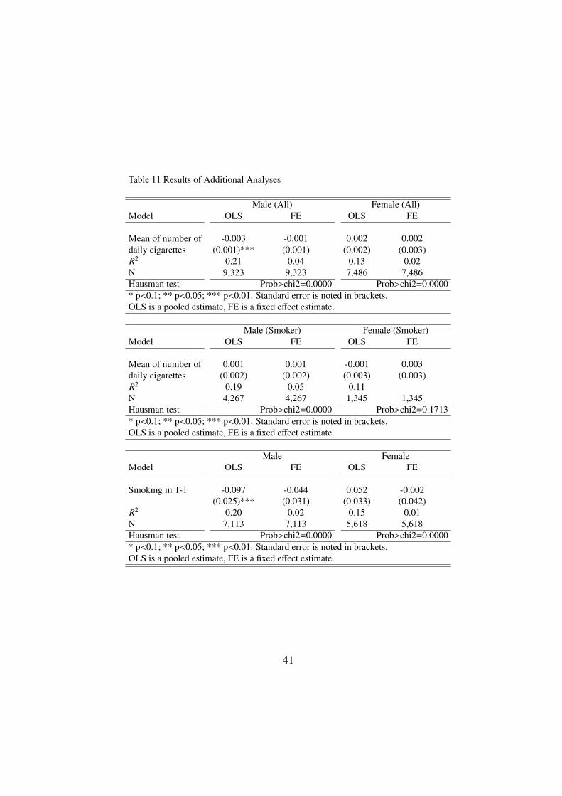
Table 11 Results of Additional Analyses
Male (All) Female (All)Model OLS FE OLS FE
Mean of number of -0.003 -0.001 0.002 0.002daily cigarettes (0.001)*** (0.001) (0.002) (0.003)R2 0.21 0.04 0.13 0.02N 9,323 9,323 7,486 7,486Hausman test Prob>chi2=0.0000 Prob>chi2=0.0000* p<0.1; ** p<0.05; *** p<0.01. Standard error is noted in brackets.OLS is a pooled estimate, FE is a fixed effect estimate.
Male (Smoker) Female (Smoker)Model OLS FE OLS FE
Mean of number of 0.001 0.001 -0.001 0.003daily cigarettes (0.002) (0.002) (0.003) (0.003)R2 0.19 0.05 0.11N 4,267 4,267 1,345 1,345Hausman test Prob>chi2=0.0000 Prob>chi2=0.1713* p<0.1; ** p<0.05; *** p<0.01. Standard error is noted in brackets.OLS is a pooled estimate, FE is a fixed effect estimate.
Male FemaleModel OLS FE OLS FE
Smoking in T-1 -0.097 -0.044 0.052 -0.002(0.025)*** (0.031) (0.033) (0.042)
R2 0.20 0.02 0.15 0.01N 7,113 7,113 5,618 5,618Hausman test Prob>chi2=0.0000 Prob>chi2=0.0000* p<0.1; ** p<0.05; *** p<0.01. Standard error is noted in brackets.OLS is a pooled estimate, FE is a fixed effect estimate.
41

them. The panel data used in this study enables lag variables for smoking behavior
in a previous year.25 The OLS estimate for males, in the third results in Table 11,
shows that smoking behavior in the prior year reduces hourly wages 9.7%, while
the FE estimate show no statistically significant results. For females, both the
OLS and FE estimates show no causal relationship between smoking behavior in
the prior year and hourly wages. Thus, we know that previous smoking behavior
does not affect hourly wages for either gender.
In this part, we examined the effects of number of cigarettes and past smok-
ing behavior on current hourly wages. The results indicate that both number of
cigarettes and past smoking behavior have no effect on hourly wages, indicating
that all of our previous results are robust.
2.6 Discussion
2.6.1 Alcohol Consumption
In this section, we discuss the relationship between smoking and alcohol con-
sumption. Generally, when we look at the literature related to the causal rela-
tionship between health and labor market outcomes, we find that researchers dis-
cuss the relationship between wages and smoking and between wages and alcohol
consumption together (Auld 2005, Lye 2004). Alcohol consumption is also an im-
portant addictive behavior in medical science. Auld (2005) provides a model that
25 Though we can take lag variables for eight years because the panel data covers 9 years, weuse lag variables for the year prior in the analysis to consider multicollinearity.
42

includes alcohol consumption patterns and controls for smoking as an endogenous
variables to investigate the effect of alcohol consumption and smoking on income
using cross-sectional data (the Canadian General Social Survey, 1985 and 1991).
The results show that “moderate drinking leads to 10% greater income than drink-
ing abstention” and “smokers earn 8% less than non-smokers” (Auld 2005). Our
study indicates similar results for male smoker in the OLS model (9.4%).
Regarding alcohol consumption behavior, Table 12 shows the descriptive statis-
tics of alcohol consumption attribution by smoking status.26 Although many
smokers drink alcohol (82% for male and 67% for female), non-smokers also have
a similar rate of alcohol consumption behavior, especially for male respondents
(78%). In terms of alcohol consumption frequency, most smokers tend to drink
more than three times a week than non-smokers do, and most non-smokers tend
to drink once or twice a month. Table 12 also shows the correlation coefficients of
smoking and alcohol consumption, which indicates a statistically significant but
low positive correlation between smoking and alcohol consumption. Addition-
ally, the correlation between hourly wages and alcohol consumption and between
hourly wages and smoking for males have similar influences, though smoking is
negative and alcohol consumption is positive, indicating that the effect of alcohol
consumption on wages may be similar to the effect of smoking on wages estimated
in this section using this sample data.
26 At the KHPS miss the data of drinking attribution in 2004 and 2007, the sample size is smallerthan Table 2.
43

Tabl
e12
Des
crip
tive
Stat
istic
san
dC
orre
latio
nof
Alc
ohol
Con
supt
ion
Mal
eFe
mal
eSm
oker
Non
smok
erSm
oker
Non
smok
erD
escr
iptiv
eSt
atis
tics
(Mea
n)D
rink
ing
0.81
50.
784
0.66
80.
524
Dri
nkon
ceor
twic
ea
mon
th0.
189
0.20
00.
240
0.28
4D
rink
once
ortw
ice
aw
eek
0.10
80.
154
0.11
10.
099
Dri
nkm
ore
than
thre
etim
esa
wee
k0.
519
0.43
00.
317
0.14
2N
3068
3795
1000
4619
Mal
eFe
mal
eSm
okin
gD
aily
num
ber
Hou
rly
Smok
ing
Dai
lynu
mbe
rH
ourl
yof
ciga
rette
sw
ages
ofci
gare
ttes
wag
esC
orre
latio
nD
rink
ing
0.03
9***
0.02
00.
048*
**0.
111*
**0.
080*
**0.
034*
*D
rink
once
ortw
ice
am
onth
-0.0
15-0
.038
***
-0.0
10-0
.037
***
-0.0
37**
*0.
017
Dri
nkon
ceor
twic
ea
wee
k-0
.068
***
-0.0
81**
*0.
033*
**0.
016
-0.0
090.
002
Dri
nkm
ore
than
thre
etim
esa
wee
k0.
089*
**0.
101*
**0.
024*
*0.
177*
**0.
157*
**0.
024*
*p<
0.1;
**p<
0.05
;***
p<0.
01.
The
coeffi
cien
tofc
orre
latio
nva
lues
ofsm
okin
gan
dho
urly
wag
esis
-0.0
59**
*fo
rmal
ean
d-0
.007
6fo
rfem
ale.
44

Though we have data related to alcohol consumption, there is a hereditary
concern in Japan related to alcohol consumption. Genetically, humans need the
metabolic enzyme called acetaldehyde dehydrogenase (ALDH) to catalyze the
conversion of acetaldehyde ingested by alcohol into acetic acid. There are three
types of ALDH genes: GG type (efficiently processes a high volume of alcohol),
AG type (low ability to process alcohol) and AA type (inability to process al-
cohol). All Caucasoid (of European descent) and Negroid (of African descent)
have the GG type, but Mongoloid (of Asian descent) have all types (45% of Mon-
goloids have AG type, and 5% have AA type). According to Harada (1999), there
is a low percentage of people with the GG-type gene (NN type in Harada 1999)
especially around western Japan, indicating that estimates would have selection
bias.27 Given this concern, it is necessary to have a variable available to control
genetic selection bias, but this is difficult in the sample data we used. Thus, we
analyzed only the effect of smoking on wages in this study.
2.6.2 Exercise
Although we find there is no evidence proving that smoking is a factor deter-
mining wages in Sections 2.4 and 2.5, smoking may be a proxy of some unobserv-
able individual heterogeneity, such as personality, which affects wages. If myopic-
style thinking and smoking have a strong relationship, and most of smokers tend to
have myopic thinking, wage differences between smokers and non-smokers may
27 For example, only 40% of people in Mie province have the GG-type gene.
45

come from the difference in mode of thinking and not from smoking behavior,
indicating that smoking can be a proxy for myopic thinking.
How should we measure myopic thinking? Here, we suppose that people with
myopic thinking do not care about their health, and we use exercise as a proxy
for myopic thinking, assuming that those who do not exercise are not interested in
their health and have myopic thinking. Cawley (2004) focused on the relationship
between wages and obesity using the BMI to measure the effect of obesity on
wages and finds that heavier females tend to have lower earnings than their lighter
counterparts. In the KHPS, we use exercise instead of the BMI because this survey
did not record body weight information.
Table 13 shows the descriptive statistics related to exercise and the coefficient
of correlation values. The percentage of non-smokers who exercise is higher than
that of smokers for both males and females, though the gaps are small (13% for
male and 4% for female). The coefficients between smoking and exercising are
also statistically significant but small for males and statistically insignificant and
small values for females. The impact of the correlation values between exercise
and hourly wages are similar to the values between smoking and hourly wages,
though the former is positive and the latter is negative, and thus only males have
statistically significant values. This indicates that males with have high wages
also exercise and may not smoke, while females who have high wages may also
exercise and do not smoke or do not exercise and smoke. As there is no strong
uniformity among genders, it is hard to say that the decision to exercise reflects
myopic thinking or smoke for everyone.
46

Tabl
e13
Des
crip
tive
Stat
istic
san
dC
orre
latio
nof
Exe
rcis
eM
ale
Fem
ale
Smok
erN
onsm
oker
Smok
erN
onsm
oker
Des
crip
tive
Stat
istic
s(M
ean)
Exe
rcis
ing
0.26
70.
397
0.20
10.
245
Exe
rcis
eon
eda
ya
wee
k0.
128
0.16
90.
086
0.10
7E
xerc
ise
two
days
aw
eek
0.06
60.
095
0.03
90.
057
Exe
rcis
eth
ree
days
aw
eek
0.03
00.
049
0.03
70.
035
Exe
rcis
efo
urda
ysa
wee
k0.
009
0.02
20.
009
0.01
4E
xerc
ise
five
days
aw
eek
0.01
20.
025
0.00
60.
011
Exe
rcis
esi
xda
ysa
wee
k0.
006
0.01
20.
007
0.00
7E
xerc
ise
seve
nda
ysa
wee
k0.
016
0.02
40.
017
0.01
5N
3061
3786
998
4615
Mal
eFe
mal
eSm
okin
gD
aily
num
ber
wag
esSm
okin
gD
aily
num
ber
wag
esof
ciga
rette
sw
ages
ofci
gare
ttes
wag
esC
orre
latio
nE
xerc
isin
g-0
.137
***
-0.1
36**
*0.
074*
**-0
.039
***
-0.0
53**
*0.
013
Exe
rcis
eon
eda
ya
wee
k-0
.057
***
-0.0
49**
*0.
036*
**-0
.027
**-0
.035
***
0.01
3E
xerc
ise
two
days
aw
eek
-0.0
53**
*-0
.061
***
0.04
5***
-0.0
31**
-0.0
37**
*0.
012
Exe
rcis
eth
ree
days
aw
eek
-0.0
47**
*-0
.039
***
-0.0
010.
005
0.00
90.
023*
Exe
rcis
efo
urda
ysa
wee
k-0
.053
***
-0.0
49**
*0.
023*
-0.0
16-0
.022
*-0
.003
Exe
rcis
efiv
eda
ysa
wee
k-0
.049
***
-0.0
63**
*0.
012
-0.0
19-0
.016
-0.0
10E
xerc
ise
six
days
aw
eek
-0.0
32**
*-0
.040
***
0.03
7***
0.00
2-0
.001
-0.0
13E
xerc
ise
seve
nda
ysa
wee
k-0
.028
**-0
.029
**0.
013
0.00
8-0
.008
-0.0
25*
*p<
0.1;
**p<
0.05
;***
p<0.
01.
The
coeffi
cien
tofc
orre
latio
nva
lues
ofsm
okin
gan
dho
urly
wag
esis
-0.0
59**
*fo
rmal
ean
d-0
.007
6fo
rfem
ale.
47

Though it is difficult to use the KHPS data to capture some unobservable indi-
vidual heterogeneity affecting wages, personality is one possible factors determin-
ing and may cause wage differences between smokers and non-smokers. Another
area of future work should aim to identify the relationship between personality
and wages through health attributions.
2.7 Conclusion
In this chapter, we use Japanese panel data (KHPS) to examine the hypothesis
that smoking behavior reduces wage levels. In the analyses, we controlled for
time-invariant individual heterogeneity that is difficult to capture using two-year
panel data and cross-sectional data. Moreover, we examined IV estimations to
control for time-variant individual heterogeneity and conducted several analyses
to check robustness.
All results show that wage differences between smokers and nonsmokers come
from individual unobservable heterogeneity. The OLS estimates indicate that
smoking males have 9.4% lower hourly wages than nonsmokers, while the FE es-
timates show no statistically significant effect. In other words, smoking behavior
does not affect hourly wages if we control for individual unobservable heterogene-
ity and find that people would not see an increase in wages if they quit smoking.
Females show different results from males, having no statistically significant re-
sults in both the OLS and FE estimates. In sum, there is no causal relationship
between smoking behavior and wages for both males and females, though only
48

males have wage differences by smoking status from individual unobservable het-
erogeneity.
Other analyses, such the IV estimation and several robustness checks have
similar results. We use tobacco tax increases as the IV model, but have no statisti-
cally significant results in the estimations. We also examined several estimations
adding the dummy variables of company size and occupation, providing separate
estimates by employment status, using number of cigarettes smoked, and replac-
ing present smoking status with prior smoking status. After adding company size
and occupation, the coefficient of smoking status has small changes, but still in-
dicates no causal relationship between smoking behavior and hourly wages. The
robustness checks yielded similar results.
This chapter illustrates that wage differences by smoking status arise from
individual unobservable heterogeneity and not from the smoking behavior itself.
However, smoking undeniably has a negative effect on labor productivity through
its impact on health, which leads to wage changes in the long term. To examine
this mechanism, future research will require a much longer panel data survey.
49

References[1] Auld, M. C. (2005) “Smoking, Drinking, and Income.” The Journal of Hu-
man Resources. 40(2), 505-518.
[2] Ault, R. W., R. B. Ekelund Jr J. D., Jackson, R. S. Saba, and D. S. Saurman(1991) “Smoking and Absenteeism.” Applied Economics. 23, 743-754.
[3] Barik, J. and S. Wonnacott (2009) “Molecular and Cellular Mechanisms ofAction of Nicotine in the CNS.” Handbook of Experimental Phamacology.192, 173-207.
[4] Benowitz, N. L. (2008) “Neurobiology of Nicotine Addiction: Implica-tions for Smoking Cessation Treatment.” The American Journal of Medicine.121(4A), S3-S10.
[5] Benowitz, N. L. (2010) “Nicotine Addiction.” New England Journal ofMedicine. 362 (24), 2295-2303.
[6] Bush, R. and M. Wooden (1995) “Smoking and Absence from Work: Aus-tralian Evidence.” Social Science & Medicine. 41(3), 437-446.
[7] Cawley, J. (2004) “The Impact of Obesity on Wages.” The Journal of HumanResources. 39(2), 451-474.
[8] Cornwell, C. and P. Rupert (1997) “Unobservable Individual Effects, Mar-riage and the Earnings of Young Men.” Economics Inquiry. 35, 285-94.
[9] Gray, J. S. (1997) “The Fall in Men’s Return to Marriage: Declining Produc-tivity Effects of Changing Selection?.” The Journal of Human Resources. 32,481-504.
[10] Hackshaw, A. K., M. R. Law, and N. J. Wald (1997) “The Accumulated Evi-dence of Lung Cancer and Environmental Tabacco Smoke.” British MedicalJournal. 315, 980-988.
[11] Harada, S. (1999) “Inshu Kodo to Idenshi” (Drinking Behavior and Genes).Koshueisei. 63(4), 234-237.
[12] Institute for Health Economics and Policy (2010) “Kinen Seisaku noArikata ni Kansuru Kenkyu—Kitsuen ni yoru Cost Suikei—Hokokusho”
50

(The report of the quality of the tobacco cessation policy―Cost estimate onSmoking). http://www.ihep.jp/publications/report/search.php?dl=26&i=1(accessed July 15, 2013).
[13] Ishii, K. and H. Kawai (2006) “Tabakozei no Hikiage ya Kenkozoshinho waKinen ni Dokomade Yuko ka” (The Validity of the Cigarette Tax Hike andthe Health Promotion Act). Y. Higuchi and The 21 Century COE Programs(Ed.) ”The Dynamism of Japanese Household Behavior 2.” 211-236, KeioUniversity Press.
[14] Juntendo University Respiratory “Haigan nit suite” (About Lung Cancer).http://www.juntendo.ac.jp/hospital/clinic/kokyukigeka/kanja02_01.html(accessed November 30, 2013)
[15] Kawaguchi, A. (2008) Gender Keizai Kakusa (Gender Inequality in Eco-nomic Status). Keiso Shobo.
[16] Kawai, H. (2012) “2010 Nen Tabakozei Hikiage no Koka—JHPS ni yoruPanel Data Bunseki” (The effect of 2010 Cigarette Tax Hike―Panel Anal-ysis of JHPS), Y. Higuchi, T. Miyauchi, C. R. McKenzie, and Panel DataResearch Center at Keio University (Ed.) The Dynamism of Parent-child Re-lation and Family Behavior―Education, Health and Employment under Fi-nancial Crises. 105-124, Keio University Press.
[17] Kitamura Y. (2005) Panel Data Bunseki (Panel Data Analysis), IwanamiShoten.
[18] Leigh, P. J. (1995) “Smoking, Self-selection and Absenteeism.” QuarterlyReview of Economics and Finance. 35, 365-386.
[19] Levine, P. B., T. A. Gustafson, and A. D. Velenchik (1997) “More Bad Newsfor Smokers? The Effects of Cigarette Smoking on Wages.” Industrial andLabor Relations. 50(3), 493-509.
[20] Lye, J. N. and J. Hirschberg (2004) “Alcohol Consumption, Smoking andWages.” Applied Economics. 36, 1807-1817.
[21] The Ministry of Health, Labour and Welfare “Saishin Tobacco Joho: SeijinKitsuen Ritsu (Kousei Roudou Sho Kokumin Eiyo Chosa)” (The Newest
51

Tobacco Information: Adult Smoking Rate (The National Nutrition Sur-vey by The Ministry of Health, Labour and Welfare)). http://www.health-net.or.jp/tobacco/product/pd100000.html (accessed September 30, 2013).
[22] The Ministry of Health, Labour and Welfare “Saishin Tobacco Joho:Seijin Kitsuen Ritsu (Kousei Roudou Sho Kokumin Eiyo Chosa)” (TheNewest Tobacco Information: Adult Smoking Rate (The Survey of JapaneseSmoking Rate by Japanese Tobacco Incorporated)). http://www.health-net.or.jp/tobacco/product/pd090000.html (accessed September 30, 2013).
[23] The National Cancer Center “Tobacco to Shibo Ritsu tono Kankeini tsuite” (The Relationship Between Smoking and Death Rate),http://epi.ncc.go.jp/jphc/outcome/252.html (accessed November 30, 2013).
[24] The World Bank (1999) “Tobacco Ryuko no Yokusei” (Restraint of Smok-ing). A World Bank Publication.
[25] Uemura, K and A. Noda (2011) “Kitsuen Shukan no Panel Bunseki—Goriteki Izonsho Model no Kensho” (The Panel Analysis of Smoking Habit―Test of The Rational Addiction Model). M. Seko, H. Teruyama, I. Ya-mamoto, Y. Higuchi, and The 21 Century COE Program (Ed.) The Dy-namism of Japanese Household Behavior 7. 91-110, Keio University Press.
[26] Wooldridge, J. M. (2010) Econometric Analysis of Cross Section and PanelData second Edition. The MIT Press.
[27] Yuda, M. (2010) “Kenko Jotai to Rodo Seisansei” (Health Status and LaborProductivity). The Japanese Journal of Labour Studies. 601, 25-36.
[28] Yuda, M. (2011) “The Effect of Habitual Smoking on Labour Productivity.”Applied Economics Letters. 18, 1125-1132.
[29] Yuda, M. (2012) “Tobacco ni Taisuru Juyo・Kyokyu Shock ga Kitsuen Kodoni Ataeta Eikyo” (The effect of Tobacco Demand and Supply Shocks onSmoking Behavior). Japanese Journal of Health Economics & Policy. 24(2),143-156.
[30] Yuda, M. (2013) “The Impact of Recent Smoking Control Policies on In-dividual Smoking Choice: The Case of Japan.” Health Economics Review.Vol.3, Article 4.
52

3 Chapter 3 Men’s Wages and Intra-household
Specialization
3.1 Introduction
A considerable number of studies have been conducted over the past few
decades examining the effect of marital status on an individual’s wage level. Sev-
eral studies using cross-sectional data found a positive effect of over 10% on male
wage levels as a result of marriage (Antonovics and Town 2004; Ginther and Za-
vodny 2001; Korenman and Neumark 1991). Does marriage itself cause increased
earnings for males, or are there other determining factors affecting male wages as-
sociated with marital status?
One famous hypothesis that explains wage disparities in marital status is called
the household specialization hypothesis. According to Becker (1973; 1974; 1991),
if women have a comparative advantage over men in the household sector and men
have a comparative advantage over women in the market sector, then, specializa-
tion by each partner in each sector would have more efficient outcomes than if
both contributed in both sectors. If this hypothesis explains the mechanism of the
marriage wage premium, then males married to full-time housewives could con-
serve their time spent engaged in household tasks and spend more time at works.
By getting married, males would increase their earnings compared to males with
working wives and single males.
53

Only few related studies analyze the relationship between marriage and male
work hours as most studies focus on the change in housework hours after marriage
or a wife’s work hours (Bardasi and Taylor 2008; Gray 1997; Hersch and Stratton
1997). Using panel data (the Panel Study of Income Dynamics 1968 to 1992),
Lundberg and Rose (2002) estimate the effects of children on male hourly wages
and work hours and find that marriage and being a father leads to higher wages and
longer work hours. Although Lundberg and Rose (2002) is not a direct analysis of
the relationship between marriage and male work hours, marriage also increases
men’s work hours. According to Lundberg and Rose (2002), Yukawa (2013) esti-
mates the effect of marriage on men’s work hours using Japanese panel data (the
Keio University Household Panel Survey from 2004 to 2012) which we use in
this chapter. After controlling for time-invariant unobservable individual hetero-
geneity, the results show married males work 112 hours more annually than single
males (statistically significant at the 10% level). According to Yukawa’s (2013)
results, in this chapter, we estimate and discuss the effect of intra-household spe-
cialization on men’s hourly wages based on the mechanism that males married to
full-time housewives save their time spent engaged in housework and spend more
time in market work which increases their earnings much more than that of males
with working wives and single males.
Many studies have used the wife’s working status or work hours as proxy vari-
ables for intra-household specialization. Using cross-sectional data (the National
Longitudinal Survey of Youth 1990), Loh (1996) finds no statistically significant
difference in male earnings according to a wife’s work hours after marriage. How-
54

ever, using the same data, Gray (1997) states that male earnings increase more
slowly if the wife continues to work after marriage in the US. After the year 2000,
panel data analyses have more supportable evidence. Hersch and Stratton (1997)
find that married males spend less time engaged in housework than single males
but conclude that the impact of marriage and time spent on housework is small,
and the differences cannot be explained by intra-household specialization in the
US and the panel data (the National Survey of Families and Households 1987 to
1988, 1992 to 1994). Bardasi and Taylor (2008) examine this topic with British
data (the British Household Panel Survey 1991 to 2003) and find that if the woman
is responsible for more domestic chores, then, her husband shows 3% greater
earnings than males whose wives are responsible for no housework. Also, using
German panel data (the German Socio-Economic Panel 1985 to 2006) Pollmann-
Schult (2011) finds that males with a non-working spouse have a higher wage
premium than males with a full-time employed spouse.
In Japan, Kawaguchi (2005) shows that unobservable individual heterogene-
ity causes male wage differences according to marital status, although the data
(the Japanese Panel Survey of Consumers 1993 to 2000) only include married
males. Sato (2012) uses the data (from the Keio University Household Panel
Survey 2004 to 2012) including both married and single males and finds that un-
observable individual heterogeneity causes differences in male wages according
to marital status. However, these two studies only consider marital status itself
and not intra-household specialization. It is difficult to find studies on the rela-
tionship between intra-household specialization and male wage rates. One reason
55

for the lack of studies on the relationship between intra-household specialization
and wage levels is that, typically, intra-household specialization only occurs after
marriage. In other words, intra-household specialization is a result of marriage.
Thus, if we cannot find any relationship between marital status and wage levels,
this may indicate that the household specialization hypothesis is rejected. How-
ever, we believe there is room to examine the relationship between intra-household
specialization and wages in Japan.
The effect of marriage on wages can be categorized in several ways, such as
short-term effect, long-term effect, and an effect that mediates other factors. When
we use only marital status to measure marriage premium, the result represents a
mixed effect of facts related to marriage. Supposing the effect of one fact, such as
intra-household specialization, has a positive but small effect on wages, the mixed
effect would disappear if other facts such as marriage duration or marital life have
a substantial negative effect. Therefore, we believe it is worthwhile to measure
the effect of facts related to marriage on male wages, separately.
Additionally, it is more important to verify the effect of intra-household spe-
cialization on male wages in Japan compared to other European countries be-
cause of the certain existence of intra-household specialization in Japan. On In-
ternational Women’s Day 2014, the Organization of Economic Cooperation and
Development reported on the time spent working by men and women in 26 coun-
tries.28 Figure 1 shows that in Japan, over 80% of unpaid work is carried out by
28 “Balancing paid work, unpaid work and leisure”http://www.oecd.org/gender/data/balancingpaidworkunpaidworkandleisure.htm(December 15,
2014)
56

women, and Japan has the second greatest unpaid work gender gap after Korea.
Additionally, according to the White Paper on the Labour Economy 2015 by the
Ministry of Health, Labour and Welfare, 42% of households in Japan had un-
employed wives in 2012 and, approximately, 20% of single women aged 18 to 39
hope to become housewives in the future. Of course, this may be a cultural charac-
teristic of Asian countries, but intra-household specialization occurs in Japan and
affects male wage rates more than European countries indicating that the effect
on wages between marital status and intra-household specialization is separable.
Other significant results for male wage differences by marital status may be found
in Japan.29 Yukawa (2013) is the only related study to the best of our knowledge.
This study examines the effect of marriage on labor supply for both males and fe-
males and also examines the effect of intra-household specialization on time spent
working using the difference in educational background between married couples
as a proxy variable with Japanese panel data (the Keio University Household Panel
Survey 2004 to 2012). The results show that if a husband has a higher educational
background than his spouse, the husband will work more than the spouse. This
result supports the existence of intra-household specialization in Japan according
to Becker’s hypothesis (1973; 1974; 1991).To the best of our knowledge, no study
examines the relationship between intra-household specialization and male wage
rates in Japan. We believe that this chapter has profound significance in verify-
ing wage differences between married males and single males because of marital
29 Unpaid work includes routine housework, shopping, care of household members, care ofnon-household members, volunteering, travel related to household activities, and other unpaidwork.
57

status and other marriage-related factors such as intra-household specialization.
Additionally, Kawaguchi (2005), Sato (2013), and Yukawa (2013) are written in
Japanese. We believe that this study is the first study written in English that eval-
uates the marriage wage premium according to marital status and intra-household
specialization in Japan.
In this chapter, we analyze the effect of marital status and intra-household spe-
cialization on male wages in Japan using Japanese panel data. The ordinary least
square (OLS) analysis yields a wage premium for married men of 8 to 14% and
married men with a full-time housewife shows an additional effect of 10 to 13%.
After controlling for fixed effects, the marital and intra-household specialization
effects disappear indicating that the factors causing male wage differences are
not marital status and wife’s working status. In other words, marriage and intra-
household specialization do not cause male wage differences among married men
58

with a full-time housewife and others if marital status and wife’s working status
represent marriage and intra-household specialization.
The proxy variable we used for intra-household specialization is the “current”
wife’s working status. Because a “past” wife’s working status should affect male
wages, we used a first-difference (FD) estimator to check this fact. Our results
show the robustness of the FE results. We clarify individual heterogeneous ef-
fects, which may lead to male wage differences because of marital status and the
status of working wives, focusing on heterogeneous effects across organizations
and occupations. Estimating the OLS model and fixed effect (FE) model by con-
trolling for dummy variables of large company size and occupations, or estimat-
ing separately by the size of the company, the results continuously show the same
facts. Several additional estimations also support our findings. In summary, we
state positively that not all males have higher wages after marriage or after their
wife becomes a full-time housewife. This finding indicates that no evidence of
a marriage wage premium for Japanese males is found in this study after several
in-depth empirical analyses.
The remainder of this chapter is organized as follows. Section 2 introduces
the data and presents descriptive statistics, Section 3 explains the method and
discusses the main results, and Section 4 shows the results of a robustness check.
Section 5 summarizes and concludes the study.
59

3.2 Data and Descriptive Statistics
3.2.1 Data
The data used in this analysis is the Keio University Household Panel Survey
(KHPS) from 2004 to 2012. This data contains basic annual individual infor-
mation such as working status, years of working experience, tenure, education
information, marital status, firm size and job type for approximately 4,000 indi-
viduals since 2004. Wave 2 has 1,400 individuals from 2007, and wave 3 has
1,000 individuals from 2012. The questionnaire obtained data for individuals and
their spouses so that we also obtain sufficient basic information for spouses.30
The Japanese Act concerning Stabilization of Employment of elderly persons
configured the retirement age as 60 years of age or older.31 Because of this re-
tirement requirement, income levels suddenly decline after workers with a col-
lege background reach 60 years of age, and we cannot obtain a continuous wage
function for Japanese males (Kawaguchi, 2011). Therefore, the sample data only
include working males from 20 to 59 years old. If there was a missing value in the
data, it was also removed. We limited samples for men only because of the sam-
ple selection bias for women’s wage levels. Additionally, we do not use wave 3
(2012) because wave 3 has only one year of data and does not allow us to conduct
30 Marital status cannot distinguish between legal marriage and de facto marriage. Therefore,we define marital status as “subjective” marital status in this chapter.
31 The age requirement changed to over 65 years of age after April 1, 2013.
60

a panel analysis. The average hourly wage we use is defined as the following,
hwage =Annual earnings
Hour × 52(weeks)
where Annual earnings is the year amount calculated from regular payment and
bonus information in a questionnaire, Hour represents working hours per week
including overtime work hours.32 Table 1 describes other variables.
3.2.2 Descriptive Statistics
Figure 2 describes the average hourly wage by marital status for men in each
age group. The figure shows that married males have a higher average hourly
wage particularly after they reach age 30, and the average age at which males
marry is approximately 28 years old (Table 2). Considering these facts, it seems
quite probable that wage differences by marital status dramatically increase after
an individual reaches age 30. In other words, there seems to be a higher wage level
for men after marriage, and wage differences according to marital status become
more significant with age.
32 We use the monthly income amount multiplied by 12 months for individuals who respondedthat they received income monthly or weekly. Additionally, we use a daily income amount andmultiply the amount by monthly working days and 12 months for those who received income dailyand use annual income for those who received income annually. There are two questionnairesconcerning income: “an annual income including tax” or “the highest monthly, daily, hourly, andannual income if you have more than two jobs,” and we use the latter. We establish the robustnessof the results in this chapter when we use “the number of working days per month” and multiply by12 months instead of using “working hours per week” and multiplying by 52 weeks as a robustnesscheck. We exclude the results.
61

Table 1 Variabe ExplanationExplained VariableWage per hour (JPY) Hourly wage.
Individual InformationAge Each survey year minus birth year.Marriage dummy Equal to 1 if married and 0 if single.Children Equal to 1 with a child and 0 otherwise.Children under 6 Equal to 1 with an under 6 years old and 0 otherwise.
Educational InformationYears of education Calculated from history records (15 - 68 years old).Junior high school Equal to 1 if highest graduated school is junior high school.High school Equal to 1 if highest graduated school is high school.Vocational school Equal to 1 if highest graduated school is vocational school.University Equal to 1 if highest graduated school is university.Graduate Equal to 1 if highest graduated school is graduated school.
Working InformationYears of experience Calculated from history records (15 - 68 years old).Tenure Tenure from first survey year and add or change length from
"change a job" information in each survey year.Regular worker Equal to 1 if working status is a regular worker.Company size Equal to 1 if company size is more than 500 employees.Occupations Equal to 1 if a job type corresponds to one of the following,
Agriculture, forestry and fisheries, Mining, Sales, Services,Management works, Clerical works, Transportation andtelecom works, Field works, Information technology engineer,Professional and technique works, Security, Others.Reference group is Others in estimation equations.
Change of job from last year Equal to 1 if the job changed from the previous year.Area InformationLiving in big city Equal to 1 if the city is one of 14 big cities.
Other InformationYear Dummy Equal to 1 for each year. The reference group is 2004 in estimation
equations.In the first year survey (2004), the questionnaire only used a historical questionnaire for those agedbetween 18 and 68 years old. The historical questionnaire for those aged between 15 and 17 yearsold was added in the next year (2005). We use both as one set of historical data for those agedbetween 15 and 68 years old to calculate years of education, years of experience and tenure.
62

Table 2 reports descriptive statistics for married and single males including
individual, marital, and partner information. For married males, the average wage
per hour is approximately 2,718 JPY or 1,900,000 JPY per year higher than a sin-
gle male with an average wage per hour of 1,804 JPY, which implies an observable
marriage wage premium for males in Japan.
For other variables, there is almost no difference in education years, and mar-
ried males have more experience in the labor market and longer tenure than single
males. This may be because of the average age difference between married and
single individuals, and it is one possible reason for wage differences according to
marital status. To eliminate this effect, we controlled for years of experience and
tenure in estimations.
Both married men and single men have a similar distribution of educational
63

backgrounds. Almost 40 to 45% of men are high school graduates, and 34% are
university graduates. Married males are composed of approximately 2% more
junior high school graduates, and single males are composed of approximately
2.3% more vocational school graduates and 1% more graduate school graduates.
We find that educational background does not affect wage differences according
to marital status. Despite this, we still controlled for education years for the return
on wages from education.
In Table 2, approximately 33.5% of wives are full-time housewives. “Other”
wives study and care for family members and convalescents. Almost 35% of
wives are non-regular workers, and 26.5% of wives are regular workers. Non-
regular workers include part-time workers, contract workers, contingent workers,
and temporary workers.
The descriptive statistics for males by the working status of their wives are
shown in Table 3.33 With respect to hourly wages, males have higher wages if their
wives are engaged in full-time housework compared to males whose wives work
outside the home or otherwise. Particularly, once males reach their 30s, Figure
3 indicates that intra-household specialization may increase male wage levels.
However, we also consider the possibility of reverse causality. A woman may
become a full-time housewife solely because her husband has a higher wage level
compared to others. This would happen simultaneously with marriage; therefore,
it is difficult to identify reverse effects. We assume this reverse causality is a time-
33 Wage differences for each age generation between males by their marital status and wife’sworking status are shown in Figure 3.
64

Table 2 Descriptive Statistics by Marital StatusMen
Married SingleMean SD Mean SD
Explained VariableWage per hour (JPY) 2784.388 3018.342 1836.550 2106.686
Individual AttributesAge 45.466 8.541 36.742 10.439Duration of marriage 17.343 8.882Age of getting marriage 28.166 4.779Children 0.890 0.313 0.054 0.225Children under 6 0.244 0.430 0.001 0.034
Educational AttributesYears of education 13.686 2.941 13.798 2.891Junior high school 0.037 0.188 0.033 0.178High school 0.448 0.497 0.428 0.495Vocational school 0.073 0.260 0.090 0.287University 0.362 0.481 0.339 0.473Graduate school 0.043 0.203 0.056 0.231
Work AttributesYears of experience 24.938 9.214 15.868 11.062Tenure 14.949 11.013 6.836 7.619Regular worker 0.202 0.401 0.210 0.407Company size > 500 employees 0.309 0.462 0.231 0.422Change of job from last year 0.039 0.193 0.078 0.268
Area AttributesResidence in a big city 0.274 0.446 0.285 0.451
Working status of WifeFull-time housewife 0.335 0.472Others 0.048 0.214Irregular worker 0.352 0.478Regular worker 0.265 0.441
N 5,642 1,770
65

invariant effect (supposing every female maintains a constant possibility to be a
full-time housewife throughout her life). Therefore, we used a fixed effects model
to control for this endogeneity.
Table 3 Descriptive Statistics by Wife’s Working StatusMen
Full-time housewife Other working status*Mean SD Mean SD
Explained VariableWage per hour (JPY) 2946.004 2800.091 2702.848 3119.858
Individual AttributesAge 43.342 8.975 46.537 8.106Duration of marriage 15.071 8.789 18.489 8.707Age of getting marriage 28.311 4.397 28.093 4.960Children 0.931 0.253 0.869 0.337Children under 6 0.421 0.494 0.155 0.362
Educational AttributesYears of education 14.141 3.096 13.457 2.833Junior high school 0.023 0.149 0.044 0.205High school 0.405 0.491 0.47 0.499Vocational school 0.063 0.244 0.078 0.268University 0.402 0.49 0.342 0.475Graduate school 0.078 0.269 0.025 0.157
Work AttributesYears of experience 22.405 9.549 26.215 8.768Tenure 14.543 10.507 15.153 11.256Regular worker 0.209 0.407 0.198 0.398Company size > 500 employees 0.351 0.477 0.287 0.453Change of job from last year 0.038 0.191 0.039 0.193
Area AttributesResidence in a big city 0.341 0.474 0.239 0.427
N 1,892 3,750* Wives are engaged in work, study, caring, and not involving housework.
66

Table 4 shows the transition matrix for males. The upper matrix shows the
change in marital status, and the lower matrix shows the change in a wife’s work-
ing status. A total of 5.11% of males changed their marital status from single to
married according to these data, which is a sufficient marital change rate com-
pared to the Japanese marriage change rate at 5.2% per 1,000 of the population,
according to Japanese national vital statistics for 2014 for all age groups.34 We be-
lieve this marital change rate is sufficient for the fixed effect model. The difference
between the KHPS and the national data may be caused by the differences in the
included generations (all generations in the national data and 20 to 59 year olds in
the estimated sample in this paper) and a non-random attrition problem with the
34 The divorce rate is approximately 0.6% from our sample data in Table 4 while it is ap-proximately 1.7% per 1,000 of the population according to the national vital statistics in 2014.Additionally, the sample size of newly divorced men is small. It is effective to remove this sampleto distinguish the marriage premium from the divorce premium. This can be one of the robustnesschecks.
67
KHPS. One future work is to control this attrition problem to review the robust-
ness of previous studies.35 Regarding the wife’s working status, approximately
8.33% of wives quit their job or changed their working status to full-time house-
wife once married.36 Additionally, approximately 19.53% of wives start work or
commit to other responsibilities, such as caring for family members, rather than
assuming full-time housework. We consider this transit rate to be sufficient for a
fixed effect model.
3.3 Intra-household Specialization and Wage Premium
3.3.1 Empirical Methodology
For the intra-household specialization effect, we use the interaction term for
marriage and wife’s working status as a proxy variable.
In line with Wooldridge (2010), the estimation equation is the following Min-
cer equation,
ln(hwageit ) = α + β1(Marriage)it + β2(Duration o f Marriage)it
+ (Marriage ×Working status o f wi f e)it β3 + Xit β4 + β5dt + ci + vit (1)
35 One method to control for sample attrition bias is to use weighting to render the KHPS andthe national data comparable. However, there is no comparable national data, and we decided toleave this problem for the future work.
36 It is difficult to find a related national statistic. One possible statistic is in the White paper in2015 by the Ministry of Health, Labour and Welfare in which we know there are approximately8.7% of single women aged from 18 to 39 years old who intend to be a full-time housewife in2010.
68

Table 4 Transition Matrix of MalesT + 1
Single Married Total0 1
Single 1,243 67 1,310 N0 94.89 5.11 100 %
TMarried 27 4,311 4,338 N
1 0.62 99.38 100 %
Total 1,270 4,378 5,648 N22.49 77.51 100 %
T + 1Other work* Housework** Total
0 1
Other work 2,586 235 2,821 N0 91.67 8.33 100 %
THousework 291 1,199 1,490 N
1 19.53 80.47 100 %
Total 2,877 1,434 4,311 N66.74 33.26 100 %
* Wives are engaged in work, study, caring, and not involvinghousework.
** Wives are full-time housewives.
69

where ln(hwageit ) is the log of the hourly wage for individual i in time t; Marriage
is a dummy variable equal to one if married; Duration o f Marriage is the du-
ration of marriage for each married male: Marriage ×Working status o f wi f e
is the interaction term of marriage and the working status of the wife; X is a
vector of individual attribution such as years of education; working experience
and tenure; d is a year dummy; c is unobservable individual information, and the
random variable v is an error term.37
The marriage effect on wages can be categorized in several ways such as short-
term effect, long-term effect, and an effect mediating other factors. Males gain
marriage utility from marital status and their marital life. If a man experiences
comfort from living with his wife over time, for example, his wife cleans every
day and prepares well-balanced meals. Then, the husband is free to concentrate on
his work. This may lead to an increasing wage level. However, a dummy variable
for marital status will not capture this effect. To catch this time-dependent effect,
we use marriage duration as a proxy variable for the passage of time for the effect
of marriage on wages.
We categorize wives’ working status into four types: full-time housework;
others including studying, caring for family members, and job searching; non-
regular workers, and regular workers. Non-respondents for the wife’s working
37 Ginther and Zavodny (2001) show that the marriage effect on wages increases by approxi-mately 10% according to the duration of marriage in OLS estimations compared with the periodjust after marriage and the period six years after marriage. Additionally, we assume that “durationof marriage” contains a motivation or satisfaction effect from marriage and having a family.
70

status were removed from the estimated data.38 We set the interaction term for
marriage and regular workers as a basis so that the interpretation is a comparison
between the regular worker and another wife’s working status. For example, if the
coefficient of the interaction term of marriage and full-time housewives becomes
positive and statistically significant, this implies that males have higher wages if
their wives change their working status from regular worker to full-time house-
wife. This also implies that intra-household specialization causes a male wage
premium according to marital status and wife’s working status.
Typically, salaries increase rapidly, and there is more childcare support in
a large company than a smaller company. Bang and Basu (2011) remark that
“less skill-intensive industries often pay lower wages,” and the authors also find
that “employment in higher skill, higher paying industries is lower for married
women.” If an individual works for a larger company, the wage rate may be higher
than the rate with a minor company in the same industry sector. Additionally, job
type may affect a person’s wage rate. For example, if an individual is a doctor,
his wage rate may be higher than a company worker in the same age group. To
consider these possible endogeneities between company-based information and
marital status, we also use control dummy variables for company size and occu-
pation type in the following equation according to several previous studies (Loh
38 The number of removed samples is approximately 150. All data we show in tables are thedata after exclusion.
71

1996, Gray 1997, Kawaguchi 2005, Sato 2012).
ln(hwageit ) = α + β1(Marriage)it + β2(Duration o f Marriage)it
+ (Marriage ×Working status o f wi f e)it β3 + Xit β4 + β5dt
+ β6(Company size)it + (Occupation types)it β7 + ci + uit (2)
where Company size is a dummy variable for company size equal to one if a
company has more than 500 employees and is equal to zero otherwise including
the civil service. Occupation types are dummy variables equal to one if a job
type corresponds to a job type shown in Table 1. The reference group is “Others.”
The random variable u is an error term.
3.3.2 Empirical Results and Discussion
Table 5 summarizes the results. Results (1) to (3) are OLS estimates, and
results (4) to (6) are FE estimates. Appendix Table 1 shows the full results of
Table 5 of both the OLS and FE estimates.
OLS estimates in result (1) are from equation (1) without the interaction term
of marital status and wife’s working status. The results show that married males
have a 13.6% higher hourly wage than single males. Result (2) shows that the
effect of marital status on wages decreases (7.8%) compared to result (1), and a
male married to a full-time housewife has a 13.5% higher hourly wage rate than a
married male with a regular working wife. This implies that males married to full-
72
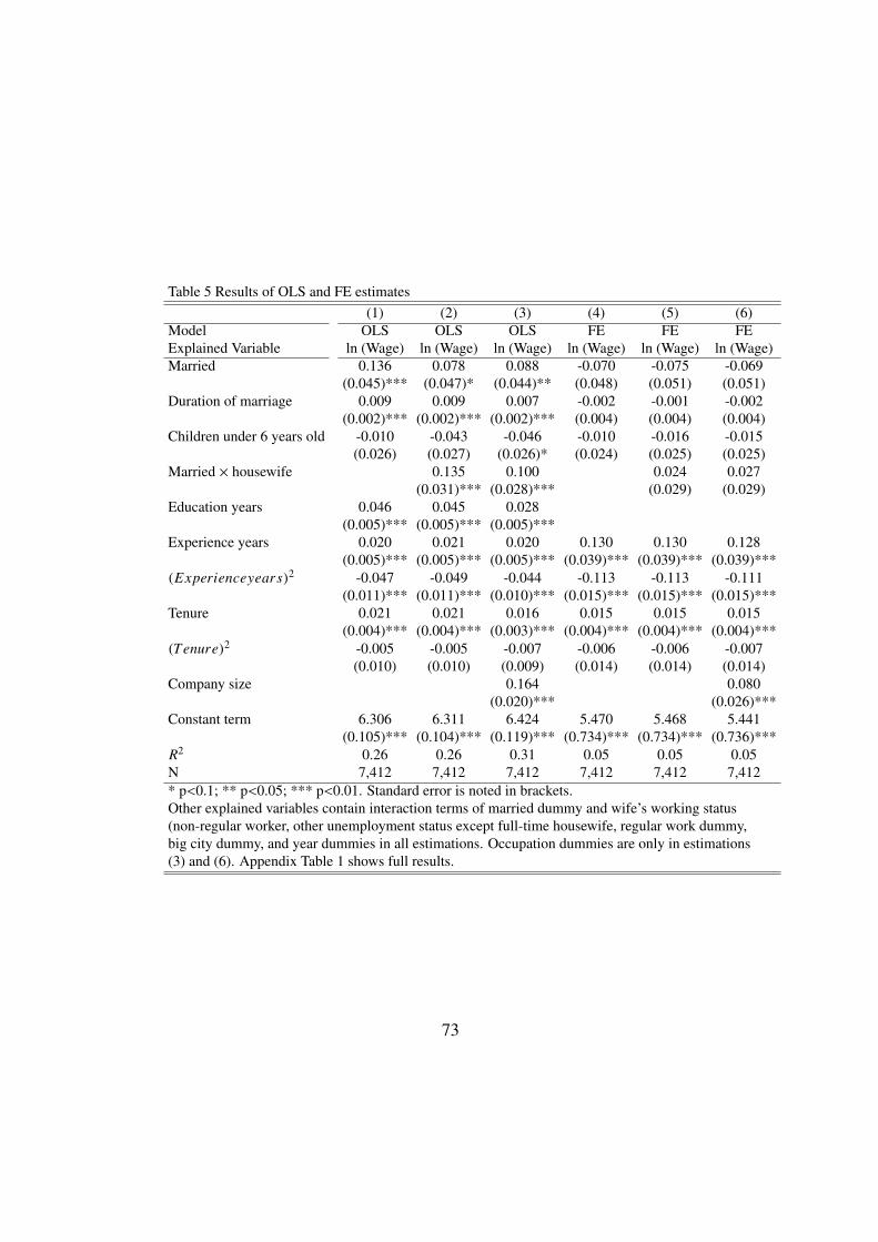
Table 5 Results of OLS and FE estimates(1) (2) (3) (4) (5) (6)
Model OLS OLS OLS FE FE FEExplained Variable ln (Wage) ln (Wage) ln (Wage) ln (Wage) ln (Wage) ln (Wage)Married 0.136 0.078 0.088 -0.070 -0.075 -0.069
(0.045)*** (0.047)* (0.044)** (0.048) (0.051) (0.051)Duration of marriage 0.009 0.009 0.007 -0.002 -0.001 -0.002
(0.002)*** (0.002)*** (0.002)*** (0.004) (0.004) (0.004)Children under 6 years old -0.010 -0.043 -0.046 -0.010 -0.016 -0.015
(0.026) (0.027) (0.026)* (0.024) (0.025) (0.025)Married × housewife 0.135 0.100 0.024 0.027
(0.031)*** (0.028)*** (0.029) (0.029)Education years 0.046 0.045 0.028
(0.005)*** (0.005)*** (0.005)***Experience years 0.020 0.021 0.020 0.130 0.130 0.128
(0.005)*** (0.005)*** (0.005)*** (0.039)*** (0.039)*** (0.039)***(Experienceyears)2 -0.047 -0.049 -0.044 -0.113 -0.113 -0.111
(0.011)*** (0.011)*** (0.010)*** (0.015)*** (0.015)*** (0.015)***Tenure 0.021 0.021 0.016 0.015 0.015 0.015
(0.004)*** (0.004)*** (0.003)*** (0.004)*** (0.004)*** (0.004)***(Tenure)2 -0.005 -0.005 -0.007 -0.006 -0.006 -0.007
(0.010) (0.010) (0.009) (0.014) (0.014) (0.014)Company size 0.164 0.080
(0.020)*** (0.026)***Constant term 6.306 6.311 6.424 5.470 5.468 5.441
(0.105)*** (0.104)*** (0.119)*** (0.734)*** (0.734)*** (0.736)***R2 0.26 0.26 0.31 0.05 0.05 0.05N 7,412 7,412 7,412 7,412 7,412 7,412* p<0.1; ** p<0.05; *** p<0.01. Standard error is noted in brackets.Other explained variables contain interaction terms of married dummy and wife’s working status(non-regular worker, other unemployment status except full-time housewife, regular work dummy,big city dummy, and year dummies in all estimations. Occupation dummies are only in estimations(3) and (6). Appendix Table 1 shows full results.
73

time housewives have a 13.5% higher hourly wage than males married to regular
working wives. The sum of both effects is 21.3% indicating that a man married
to a full-time housewife has an hourly wage that is 21.3% higher than a man
who is single. Result (3), which includes the company size and occupation type
dummies, shows a higher marital effect (8.8%) and a lower full-time housewife
effect (10%) than result (2). The sum of these effects (18.8%) is lower than result
(2) (21.3%). This indicates that equation (1) over-estimated the effect of a full-
time housewife and the sum of the marriage-related effect. Comparing result (1)
to result (3), we find that the effect of company size and occupation type mediates
the effect of marital status and wife’s working status on male wage levels. We
also find that if males have a marriage duration that is one year longer, males
have a 0.9% higher hourly wage from results (1) and (2). After controlling for
company size and occupation types, the effect is reduced to 0.7% in result (3).
Therefore, company size and occupation type could mediate marriage duration
also. In sum, OLS estimates show that marital status and a wife’s working status
represent marriage and intra-household specialization and other factors such as
working for a large company.
With respect to other variables, if males have one more year of education, they
earn, approximately, a 4.5% higher hourly wage in results (1) and (2) and a 2.8%
higher wage after controlling for company size and occupation types in result (3).
Tenure also shows similar findings in results (1) to (3), but years of experience
does not change in any of the results.39 Regardless of each result, education,
39 If a male has one more year working in the same company, his wage would increase by 2.1%,
74

working experience, and company size affect wage levels, and this is consistent
with the existing empirical evidence.
Even if the OLS results show a positive and statistically significant marriage-
related effect on wages, FE estimates show no statistically significant results. Note
that this result indicates that no wage differences are observed when males change
their marital status or when their wives change their working status and do not
indicate that there are no wage differences between married men and single men.
Additionally, three coefficients for marital status became negative. It is difficult to
interpret the meaning because the sample data consists of both males who married
and males who divorced during the experimental periods. As the effect on wages
would be different among married and divorced males, in the following section,
we separate the samples into two: single, married, and newly married males; sin-
gle, married, and newly divorced males as a robustness check.
The coefficient of the interaction term for married and full-time housewives is
still positive but smaller than the OLS estimation and not statistically significant.
It is also difficult to interpret the meaning because the sample data consists of
wives changing their work from full-time housework to other work (regular work,
non-regular work and others) and, conversely, there are 24 patterns. Therefore,
we simply assume that these FE results indicate that a change in working status of
wives does not cause male wage disparities.
The effect of marriage duration also disappeared in the FE estimates. The
but 1.6% after controlling for company size and job type. However, if a male has one more year ofexperience in the labor market, he would have approximately a 2% higher wage level regardlessof company size and job types.
75

effect of years of experience, tenure, and company size decreased compared to
OLS estimations but were still positive and statistically significant.
Although housewives have a partial effect on male wages in the OLS esti-
mates, the fixed effect model showed that most factors causing wage differences
depend on the change in marital status, and a wife’s working status show some
unobserved individual heterogeneity.40 In short, men who may be particularly at-
tractive, competent, or who possess some other characteristic that is unobserved
in the data might be appreciated more by a boss or a potential spouse leading
to both marriage and a higher wage. In addition, a woman may become a full-
time housewife because of her husband’s high wage or cultural observance. This
result implies that these possible potential factors do affect male marriage wage
premiums instead of marriage itself or intra-household specialization in Japan.
3.4 Robustness Check
3.4.1 Subsample Analysis
As the full sample contains both newly married males and newly divorced
males, the FE results of marital status mix the effect of changing marital status
from single to married (marriage) and from married to single (divorce). In order
to distinguish the mixed effect of marriage and divorce, the sample was separated
40 Korenman and Neumark (1991), Cornwell and Rupert (1995), Loh (1996), Gray (1997),Hersch and Stratton (1997), and Sato (2012) find that the marriage wage premium reduced ordisappeared by controlling for individual time-invariant fixed effects.
76

into two parts: single, married, and newly married males; single, married, and
newly divorced males. Tables 6 and 7 provide the results.
Table 6 Results of Subsample Analysis (Single male, Married male and Newly-married male)(7) (8) (9) (10) (11) (12)
Model OLS OLS OLS FE FE FEExplained Variable ln (Wage) ln (Wage) ln (Wage) ln (Wage) ln (Wage) ln (Wage)Married 0.158 0.098 0.106 -0.040 -0.045 -0.041
(0.046)*** (0.049)** (0.046)** (0.053) (0.056) (0.056)Duration of Marriage 0.009 0.009 0.007 -0.002 -0.001 -0.002
(0.002)*** (0.002)*** (0.002)*** (0.007) (0.007) (0.007)Married × Housewife 0.134 0.099 0.021 0.024
(0.031)*** (0.028)*** (0.029) (0.029)Firm size / Job Type Dummy No No Yes No No YesR2 0.26 0.27 0.31 0.04 0.04 0.05N 7,246 7,246 7,246 7,246 7,246 7,246* p<0.1; ** p<0.05; *** p<0.01. Standard error is noted in brackets.
Table 7 Results of Subsample Analysis (Single male, Married male and Newly-divorced male)(13) (14) (15) (16) (17) (18)
Model OLS OLS OLS FE FE FEExplained Variable ln (Wage) ln (Wage) ln (Wage) ln (Wage) ln (Wage) ln (Wage)Married 0.161 0.099 0.106 -0.037 -0.040 -0.031
(0.052)*** (0.055)* (0.052)** (0.136) (0.138) (0.138)Duration of Marriage 0.008 0.009 0.007 -0.002 -0.002 -0.002
(0.003)*** (0.003)*** (0.002)*** (0.006) (0.006) (0.006)Married × Housewife 0.129 0.092 0.019 0.023
(0.031)*** (0.028)*** (0.031) (0.031)Firm size / Job Type Dummy No No Yes No No YesR2 0.26 0.27 0.31 0.04 0.04 0.05N 6,970 6,970 6,970 6,970 6,970 6,970* p<0.1; ** p<0.05; *** p<0.01. Standard error is noted in brackets.
Even when separating the effect of marriage and divorce, the estimates still
show no statistically significant results. Table 6 shows that married males have
approximately a 10 to 15% point higher hourly wage than single males, and mar-
ried males with full-time house wives have approximately 10 to 13% point higher
77

hourly wage than married males with regular working wives in the OLS estimates.
Table 7 also shows similar results (approximately 10 to 16% for marital status and
10 to 13% for housewives). Both FE estimates of marital status in Tables 6 and
7 have no statistically significant results, and the coefficients are all negative indi-
cating no wage differences observed when males change their marital status. This
supports the robustness of the results in the previous section. As the investigation
period, however, is only for the nine years, and both samples contain periods after
marriage (divorced) for only a few years, these results also indicate that marriage
does not increase male wage levels immediately or fully, indicating the absence
of causality between marriage and wages. Furthermore, these results may also
indicate there is no “temporary” wage increase (drop) from marital change.41
From these two subsample analyses, we establish that the results in Section
3.4 are robust for the nine years of panel data. It is still necessary to have a longer
period of panel data to examine the effect of marriage on wages in the long term.
3.4.2 First Difference Estimation and “Past” Wife’s Working Sta-
tus
We are concerned with the accuracy of the variable “wife’s working status.”
In the previous section, we simply used the “current” wife’s working status. We
consider that the number of years for which a wife had been a full-time housewife
41 Though the results are OLS estimations, Ginther and Zavodny (2001) show that the marriageeffect is less than 10% for males who are recently married and approximately 16 to 20% for maleswho have been married for six years.
78

might represent intra-household specialization more accurately than the current
wife’s working status. For example, a longer duration as a housewife implies
better housework and frees husbands to pursue their own careers. Thus, using the
number of years as a housewife as a proxy for intra-household specialization may
show positive results. Unfortunately, that variable is not available from KHPS.
Therefore, we apply two other models: the first-difference (FD) method or the
use of the interaction term of “current” marital status and a “past” wife’s working
status.
First, we apply the first-difference method to estimate equations (1) and (2).
In Table 8, result (19) is the FD estimate without the interaction term of marital
status and current wife’s working status, and it shows no marriage premium for
males. Results (20) to (21), which are the results with the interaction term of
marital status, current wife’s working status (20), and dummies for company size
and occupation types (21), show what other variables are the same as those of
result (19): no statistically significant results are found. Regardless of each result,
education, working experience and company size affect wage levels. Appendix
Table 2 shows the full results of Table 8.
Second, we use three interaction terms of “current” marital status and three
“past” periods of wife’s working status to examine the effect of wife’s working
status on male wages instead of the number of years as a housewife. Three in-
teraction terms are as follows: the interaction term of “current” marital status
and wife’s working status one year earlier; the interaction term of “current” mar-
ital status and wife’s working status two years earlier, and the interaction term
79

Table 8 Results of FD Estimation(19) (20) (21)
Model FD FD FDExplained Variable ln (Wage) ln (Wage) ln (Wage)Married -0.069 -0.055 -0.048
(0.078) (0.082) (0.083)Duration of marriage 0.004 0.005 0.005
(0.005) (0.005) (0.005)Children under 6 years old -0.010 -0.015 -0.014
(0.040) (0.041) (0.041)Married × housewife -0.013 -0.009
(0.040) (0.040)Married × other unemployment status 0.021 0.027
(0.046) (0.046)Married × non-regular worker -0.043 -0.039
(0.034) (0.034)Education years 0.354 0.356 0.350
(0.173)** (0.173)** (0.189)*Experience years 0.267 0.270 0.271
(0.091)*** (0.090)*** (0.090)***(Experience years)2 -0.083 -0.085 -0.084
(0.029)*** (0.029)*** (0.029)***Tenure 0.021 0.021 0.020
(0.009)** (0.009)** (0.009)**(Tenure)2 -0.038 -0.037 -0.035
(0.028) (0.028) (0.027)Regular worker -0.059 -0.059 -0.051
(0.072) (0.072) (0.071)Big city -0.068 -0.070 -0.076
(0.079) (0.079) (0.078)Company size 0.080
(0.035)**Constant term -0.028 -0.029 -0.023
(0.029) (0.029) (0.028)R2 0.01 0.01 0.02N 5,070 5,070 5,070* p<0.1; ** p<0.05; *** p<0.01. Standard error is noted in brackets.All variables are the difference between a variable in time t and time t-1.Other explained variables contain year dummies in all results and occupationdummies in result (21). Appendix Table 2 shows the full results for result (21).
80

of “current” marital status and wife’s working status three years earlier. Table 9
summarizes the results. Results (22) and (23) are OLS estimates and results (24)
and (25) are FE estimates. OLS estimates show that the effect of marital status on
male wages increases over time while the effect of being a housewife decreases
over time. Although OLS estimates have statistically significant results, FE es-
timates show interesting results. Over time, the effect of being a housewife on
male wages disappears, but Table 9 shows statistically significant positive results
of 5% for the effect of the occupation of a full-time housewife and 10% for the
effect of a wife’s occupation as a non-regular worker. The table indicates that
married males with a full-time housewife have a 7.3% higher hourly wage than
married males with a regular working wife and a similar percentage for married
males with a non-regular working wife at 6.2%. The effect of being a full-time
housewife may have a short-term effect on wages. Regarding Tables 9-2 and 9-3,
no statistically significant results are observed in the FE estimates indicating that
there is no effect from a change in a wife’s working status on male wages.
From these two analyses, we establish that the results in Section 3 are robust,
and there is no effect from marital status and full-time housewives on male wages.
3.4.3 Hours Spent on Housework Among Couples
We use the number of hours that husbands spend on housework as a proxy vari-
able instead of marital status and the interaction term of marriage and the wife’s
working status. Figure 4 describes the amount of time spent on housework per
81

Table 9 Results of Estimations with "Past" Wife’s Working Status(22) (23) (24) (25)
Model OLS OLS FE FEExplained Variable ln (Wage) ln (Wage) ln (Wage) ln (Wage)9-1. T × T-1Married 0.067 0.081 -0.077 -0.066
(0.052) (0.050) (0.064) (0.064)Duration of marriage 0.007 0.005 -0.002 -0.002
(0.003)*** (0.002)** (0.006) (0.006)Married × housewife* 0.183 0.145 0.073 0.073
(0.034)*** (0.031)*** (0.036)** (0.036)**Married × other unemployment status* 0.125 0.120 0.069 0.068
(0.052)** (0.050)** (0.046) (0.046)Married × non-regular worker* 0.092 0.066 0.063 0.062
(0.032)*** (0.029)** (0.033)* (0.033)*R2 0.27 0.32 0.03 0.03N 5,070 5,070 5,070 5,0709-2. T × T-2Married 0.125 0.134 -0.001 0.013
(0.058)** (0.055)** (0.079) (0.079)Duration of marriage 0.005 0.003 0.002 0.001
(0.003)* (0.003) (0.008) (0.008)Married × housewife 0.160 0.125 -0.016 -0.012
(0.037)*** (0.034)*** (0.041) (0.041)Married × other unemployment status 0.162 0.155 0.045 0.053
(0.059)*** (0.055)*** (0.053) (0.053)Married × non-regular worker 0.066 0.038 -0.016 -0.013
(0.036)* (0.032) (0.039) (0.039)R2 0.26 0.31 0.02 0.03N 3,782 3,782 3,782 3,7829-3. T × T-3Married 0.167 0.183 0.034 0.041
(0.065)** (0.061)*** (0.107) (0.107)Duration of marriage 0.003 0.002 0.004 0.002
(0.003) (0.003) (0.010) (0.011)Married × housewife 0.152 0.116 -0.017 -0.013
(0.040)*** (0.037)*** (0.050) (0.050)Married × other unemployment status 0.114 0.086 -0.049 -0.053
(0.066)* (0.062) (0.065) (0.065)Married × non-regular worker 0.081 0.056 0.037 0.039
(0.040)** (0.037) (0.047) (0.047)R2 0.25 0.31 0.02 0.03N 2,729 2,729 2,729 2,729* p<0.1; ** p<0.05; *** p<0.01. Standard error is noted in brackets.Other explained variables contain education years in results (22), experience years andits square, tenure and its square, regular worker dummy, big city dummy and year dummies,in all results. Dummies of company size and occupation types are in estimations (23) and (25).We exclude other full results. 82

year for married couples according to a wife’s working status. Housewives spend
approximately 2,100 hours per year (about six hours per day) on housework, and
regular working wives spend approximately 1,079 hours per year (about three
hours per day) on housework. On the other hand, married males with full-time
housewives spend 84 hours per year (about 14 minutes per day) on housework,
and married males with regular working wives spend 159 hours per year (26 min-
utes per day) on housework. Full-time housewives spend twice as much time on
housework as regular working wives, and the husbands of full-time housewives
spend half as much time on housework as husbands with regular working wives.
If this represents a difference in comparative advantage, it might represent a sub-
stitute for the wife’s working status on the effect on male wages.
We used a sample composed of nuclear families and singles who live alone
only to exclude the distribution of chores to other family members such as parents.
83

The results in Table 10 (full results in the Table 5 of the Appendix), however, show
no effect from the number of hours a wife spends on housework on the husband’s
wage levels for the FE estimates although the OLS estimates are statistically sig-
nificant. When a man participates more in housework, his wage level decreases
by 14.2 to 15.2% according to the OLS estimates. The negative effects disappear
in the FE estimates. This finding is supported by the robustness results in Section
3.
Figure 4 shows obvious differences in the time spent on housework depend-
ing on marital status and a wife’s working status. It is likely that the time spent
on housework by a wife may not transfer to the husband’s work time but to the
husband’s leisure time instead. Unfortunately, the KHPS is not a survey on time
use; therefore, it is impossible to calculate leisure times. Using a time use sur-
vey to clarify the mechanism of time use and the relationship between wages and
marriage is an opportunity for future research.
3.4.4 Company Size
In Section 3, we control heterogeneity for both wages and marital-related find-
ings and found no causality between a change in marital status and male wages
and between a change in a wife’s working status and male wages. In this sec-
tion, we examine any heterogeneous effect of marriage on male wages, such as
company size or occupation types. The Appendix Tables 1 show that there are
few occupation types that have statistically significant effects on male wages at
84
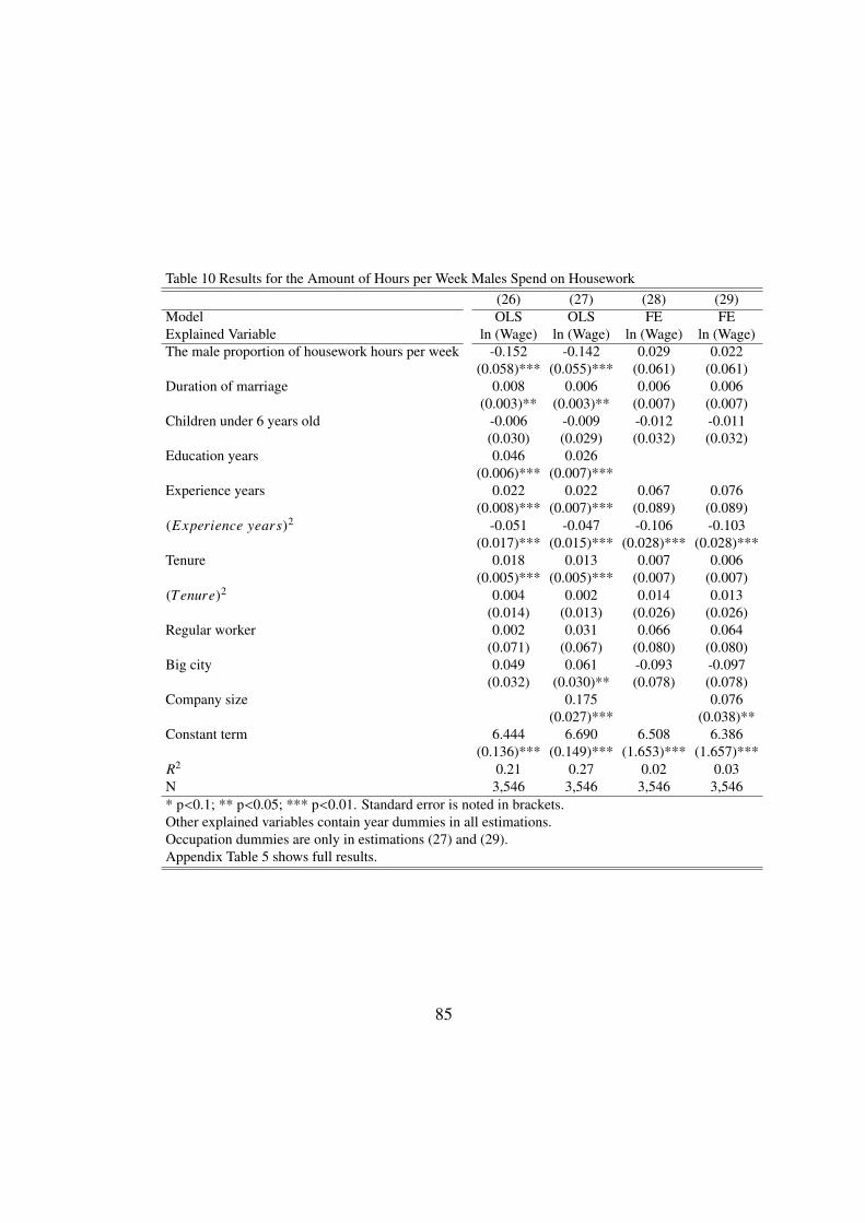
Table 10 Results for the Amount of Hours per Week Males Spend on Housework(26) (27) (28) (29)
Model OLS OLS FE FEExplained Variable ln (Wage) ln (Wage) ln (Wage) ln (Wage)The male proportion of housework hours per week -0.152 -0.142 0.029 0.022
(0.058)*** (0.055)*** (0.061) (0.061)Duration of marriage 0.008 0.006 0.006 0.006
(0.003)** (0.003)** (0.007) (0.007)Children under 6 years old -0.006 -0.009 -0.012 -0.011
(0.030) (0.029) (0.032) (0.032)Education years 0.046 0.026
(0.006)*** (0.007)***Experience years 0.022 0.022 0.067 0.076
(0.008)*** (0.007)*** (0.089) (0.089)(Experience years)2 -0.051 -0.047 -0.106 -0.103
(0.017)*** (0.015)*** (0.028)*** (0.028)***Tenure 0.018 0.013 0.007 0.006
(0.005)*** (0.005)*** (0.007) (0.007)(Tenure)2 0.004 0.002 0.014 0.013
(0.014) (0.013) (0.026) (0.026)Regular worker 0.002 0.031 0.066 0.064
(0.071) (0.067) (0.080) (0.080)Big city 0.049 0.061 -0.093 -0.097
(0.032) (0.030)** (0.078) (0.078)Company size 0.175 0.076
(0.027)*** (0.038)**Constant term 6.444 6.690 6.508 6.386
(0.136)*** (0.149)*** (1.653)*** (1.657)***R2 0.21 0.27 0.02 0.03N 3,546 3,546 3,546 3,546* p<0.1; ** p<0.05; *** p<0.01. Standard error is noted in brackets.Other explained variables contain year dummies in all estimations.Occupation dummies are only in estimations (27) and (29).Appendix Table 5 shows full results.
85

a high percentage, whereas company size has a statistically significant positive
effect on male wages even when controlling for unobservable individual hetero-
geneity. We assume that the effects of marital status or wife’s working status on
male wages are different for the employees of major and minor companies. For
example, men who are married and employed by a large company are less likely
to change jobs because they are well paid. Large company employers tend to have
more incentives to promote or train employees than smaller companies. Thus,
wage disparities occur only in a large company and not in a small company. In
this section, we use two samples according to company size: one is a company
with over 500 employees (a major company), and the other is a company with less
than 500 employees (a minor company).
Tables 11 and 12 summarize the results. Table 11 reports the results of ma-
jor companies, and Table 12 reports the results of minor companies. In Table 11,
the OLS estimates show statistically significant positive effects for marital status
and being a housewife on male wages, but the former effects disappear in Table
12 (for employees of minor companies). Although there are differences between
the effects of marital status and a wife’s working status in the OLS estimates, the
FE estimates show no effects of marital status change and a change in a wife’s
working status except for wives who change working status to or from a state of
unemployment. These estimates indicates that there is no difference in wage dis-
parities according to a change in marital status between employees of a company
with over 500 employees and a company with less than 500 employees.
86

Table 11 Results of Company Size (Over 500 Employees)Company Size (Over 500 Employees)
(30) (31) (32) (33)Model OLS OLS FE FEExplained Variable ln (Wage) ln (Wage) ln (Wage) ln (Wage)Married 0.165 0.161 -0.093 -0.085
(0.070)** (0.069)** (0.097) (0.098)Duration of marriage -0.000 -0.001 -0.002 -0.003
(0.004) (0.003) (0.007) (0.007)Children under 6 years old -0.129 -0.127 0.008 0.005
(0.045)*** (0.044)*** (0.040) (0.040)Married × housewife 0.164 0.133 -0.009 -0.006
(0.049)*** (0.046)*** (0.052) (0.052)Married × other unemployment status 0.037 0.040 -0.127 -0.117
(0.069) (0.067) (0.067)* (0.068)*Married × non-regular worker 0.064 0.042 -0.066 -0.065
(0.045) (0.044) (0.049) (0.049)Education years 0.040 0.029
(0.007)*** (0.007)***Experience years 0.017 0.014 0.078 0.072
(0.008)** (0.008)* (0.094) (0.096)(Experience years)2 -0.033 -0.022 -0.157 -0.155
(0.019)* (0.019) (0.036)*** (0.037)***Tenure 0.029 0.026 0.003 0.002
(0.007)*** (0.006)*** (0.010) (0.010)(Tenure)2 -0.021 -0.025 0.036 0.040
(0.018) (0.018) (0.032) (0.033)Regular worker 0.217 0.188 -0.068 -0.062
(0.085)** (0.087)** (0.125) (0.126)Big city 0.024 0.024 0.114 0.109
(0.034) (0.032) (0.065)* (0.066)*Constant term 6.188 6.387 6.879 6.920
(0.144)*** (0.161)*** (1.713)*** (1.736)***R2 0.34 0.37 0.07 0.08N 1,963 1,963 1,963 1,963* p<0.1; ** p<0.05; *** p<0.01. Standard error is noted in brackets.Other explained variables contain year dummies in all results.
87

Table 12 Results of Company Size (Less than 500 Employees)Company Size (Less than 500 Employees)(34) (35) (36) (37)
Model OLS OLS FE FEExplained Variable ln (Wage) ln (Wage) ln (Wage) ln (Wage)Married 0.034 0.058 -0.081 -0.073
(0.056) (0.053) (0.067) (0.068)Duration of marriage 0.012 0.010 0.005 0.003
(0.003)*** (0.003)*** (0.006) (0.006)Children under 6 years old -0.003 -0.014 -0.040 -0.036
(0.033) (0.032) (0.035) (0.035)Married × housewife 0.113 0.090 0.030 0.029
(0.037)*** (0.033)*** (0.039) (0.040)Married × other unemployment status 0.074 0.068 0.067 0.070
(0.055) (0.053) (0.049) (0.049)Married × non-regular worker 0.030 0.024 0.022 0.025
(0.036) (0.033) (0.037) (0.037)Education years 0.046 0.030
(0.006)*** (0.007)***Experience years 0.023 0.021 0.285 0.296
(0.006)*** (0.006)*** (0.065)*** (0.066)***(Experience years)2 -0.052 -0.046 -0.115 -0.114
(0.014)*** (0.013)*** (0.021)*** (0.021)***Tenure 0.018 0.015 0.015 0.015
(0.004)*** (0.004)*** (0.006)** (0.006)**(Tenure)2 -0.004 -0.011 -0.013 -0.014
(0.012) (0.012) (0.019) (0.020)Regular worker -0.026 -0.014 -0.071 -0.068
(0.063) (0.059) (0.047) (0.048)Big city 0.064 0.076 -0.111 -0.109
(0.031)** (0.030)** (0.070) (0.070)Constant term 6.253 6.391 2.300 2.058
(0.123)*** (0.142)*** (1.274)* (1.284)R2 0.22 0.26 0.04 0.04N 4,870 4,870 4,870 4,870* p<0.1; ** p<0.05; *** p<0.01. Standard error is noted in brackets.Other explained variables contain year dummies in all results.
88

3.4.5 Age Groups
Table 2 shows that the mean for marriage duration is approximately 17.3 years,
and most individuals from the data are in their 40s combined with the mean mar-
ried age for the current marriage (28 years old). Additionally, the sample size by
age groups shows that married males in their 40s and 50s account for approxi-
mately 2,000 individuals for each group, married males in their 30s account for
1,397 individuals, and married males in their 20s account for 164 individuals.
Therefore, our overall samples include more married males in their 40s and 50s.
On the other hand, the single males group has more individuals in their 20s and
30s than in their 40s and 50s.42 This sample size difference may be a possible
reason for larger wage differences according to marital status. Thus, we estimated
the equations separately by age group.
Appendix Table 4 shows the separated results for each age group. For all age
groups, we find a 7 to 24% positive effect for full-time housewives in the OLS
estimates and no statistically significant effect in the FE estimates.43 The marital
status effect on wages appeared strong only in the OLS estimates for those aged in
their 50s, but the FE estimates show no statistically significant causality between
42 Sample size by marital status and age groups: 164 (aged in their 20s and married), 1397(aged in their 30s and married), 2019 (aged in their 40s and married), 2062 (aged in their 50s andmarried), 561 (aged in their 20s and single), 590 (aged in their 30s and single), 320 (aged in their40s and single), 299 (aged in their 50s and single). The sample size by marital status is 5,642individuals for married males and 1770 individuals for single males.
43 In Appendix Table 4, the FE estimates of marital status are the following; 20s, from -22.9to -19.2%; 30s, from -0.8 to 1.7%; 40s, from -1.3 to 2.3%; and 50s, from -3.2 to 2.7%. The FEestimates of full-time housewives are the following: 20s, from 3.3 to 6.3%; 30s, from -2.4 to 1.4%;40s, 4.6%; and 50s, from 5.9 to 6.0%. All results are not statistically significant.
89

marital status and wages for all age groups.
The effect of marital status observed in Table 5 may catch up with the effect
for those aged in their 50s indicating that wage disparities according to marital
status is barely a factor caused by marriage within each group. Wage disparities,
however, are shown in Figure 2 for each group except for those aged in their 20s,
and the interaction term of marriage and full-time housewives shows statistically
significant positive results for all age groups. It is possible that this interaction
term absorbs the effect of marital status for those in their 20s to 40s in the OLS
estimates. However so, we still find no effect from marital status and a wife’s
occupation as a full-time housewife on male wages in the FE estimates (footnote
16), which is confirmed by the robustness of the results in Section 3.
3.5 Conclusion
In this chapter, we applied an intra-household specialization hypothesis to ex-
amine the reason for observed wage differences according to marital status for
Japanese men using Japanese panel data. The OLS estimates yielded a marriage
wage premium for males of 8 to 14% and males with full-time housewives had a
marriage premium of an additional 10 to 13%, results that are consistent with the
literature. However, both effects disappeared in the FE estimates, and we conclude
that the wage gap according to males’ marital status is explained by unobservable
individual heterogeneity. We conducted several subsample analyses to control for
specific and possible heterogeneity, such as the fixed effect instrumental variable
90

method, the first difference method, using “past” wife’s working status or the pro-
portion of hours males spend on housework instead of “current” wife’s working
status, and estimating models by age generation. However, we found no statisti-
cally significant positive or negative effects from any factors related to marriage
on male wages, indicating that the FE results are robust.
Although we did not find any clear evidence of the effect of intra-household
specialization on male wages, wage differences between married males and single
males are obvious. This chapter indicates that intra-household specialization is
not a factor in wage determination in Japan, and there is still room to reveal an
alternative factor that leads to wage disparities according to marital status such
as personality traits, environmental factors, or cultural characteristics. One area
for future study is to clarify the specific factors of unobservable individual hetero-
geneity affecting men’s wages and representing the relationship between marriage
and wages for women in Japan. Furthermore, it is also an important future work to
control for attrition bias of the KHPS and review the robustness of the relationship
between marriage and wages in Japan.
91

References[1] Antonovics, K. and R. Town (2004) “Are All the Good Men Married? Un-
covering the Sources of the Marital Wage Premium.” American EconomicReview. 94(2), 317-321.
[2] Bang J. T. and B. Basu (2011) “Marriage, Fertility, and the Selection ofWomen into High-Skill Industries.” Applied Economics Letters. 19(9), 829-834.
[3] Bardasi, E. and M. Taylor (2008) “Marriage and Wages: A Test of the Spe-cialization Hypothesis.” Economica. 75, 569-591.
[4] Becker, G. S. (1973) “A Theory of Marriage: Part 1.” Journal of PoliticalEconomy. 81, 813-846.
[5] Becker, G. S. (1974) “A Theory of Marriage: Part 2” Journal of PoliticalEconomy. 82, S11-S26.
[6] Becker, G. S. (1991) A Treatise on the Family. Cambridge, MA: HarvardUniversity Press.
[7] Cornwell, C. and P. Rupert (1995) “Marriage and Earnings.” Federal ReserveBank of Cleveland Economic Review. 31(4), 10-20.
[8] Ginther, D. K. and M. Zavodny (2001) “Is the Marriage Premium due to Se-lection? The Effect of Shotgun Wedding on the Return to Marriage.” Journalof Population Economics. 14, 313-328.
[9] Gray, J. S. (1997) “The Fall in Men’s Return to Marriage: Declining Produc-tivity Effects of Changing Selection?.” The Journal of Human Resources. 32,481-504.
[10] Hersch, J. and L. Stratton (1997) “Housework, Fixed Effects and Wages ofMarried Workers.” Journal of Human Resources. 32, 285-307.
[11] Kawaguchi, A. (2005) “Kekkon to Shussan wa Danjo no Chingin niDonoyona Eikyo wo Oyoboshiteirunoka” (Does Marriage and Fertility Af-fect Men and Women’s Income?). The Japanese Journal of Labour Studies.535, 42-55.
92

[12] Kawaguchi, D. (2011) “Mincer gata Chingin Kansu no Nihon no Rodoshijoheno Tekiyo” (Application to the Japanese Labor Market of the MincerWarnings Function). Current Trends in Economics 2011. Tokyo KeizaiShimpo-sha, 67-98.
[13] Korenman, S. and D. Neumark (1991) “Does Marriage Really Make MenMore Productive?. Journal of Human Resources. 26(2), 282-307.
[14] Loh, E. S. (1996) “Productivity Differences and the Marriage Wage Premiumfor White Males.” Journal of Human Resources. 31(3), 566-589.
[15] Lundberg, S. and E. Rose (2002) “The effects of sons and daughters on men’slabor supply and wages.” The Review of Economics and Statistics. 84(2),251-268.
[16] National Institute of Population and Social Security Research (2010) “The14th Japanese National Fertility Survey.”http://www.ipss.go.jp/ps-doukou/j/doukou14/doukou14.asp (accessed De-cember 6, 2015)
[17] Pollmann-Schult, M. (2011) “Marriage and Earnings: Why Do Married MenEarn More than Single Men?.” European Sociological Review. 27, 147-163.
[18] Ministry of Health, Labour and Welfare (2014) “Japanese National VitalStatistics.”http://www.mhlw.go.jp/toukei/saikin/hw/jinkou/kakutei14/index.html(accessed December 6, 2015)
[19] Ministry of Health, Labour and Welfare (2015) “The White Paper.”http://www.mhlw.go.jp/wp/hakusyo/kousei/15/ (accessed December 6,2015)
[20] Organization for Economic Co-operation and Development (OECD) (2014)“Balancing Paid Work, Unpaid Work and Leisure.” OECD Gender ofequality webpage.http://www.oecd.org/gender/data/balancingpaidworkunpaidworkandleisure.htm(accessed December 15, 2014).
[21] Sato, K. (2012) “Propensity Score Matching Ho wo Mochiita Dansei noMarriage Premium no Kensho” (Verify Male Marriage Wage Premium with
93
Propensity Score Matching) Economic and Social Research Institute Eco-nomic Analysis. 187, 47-68.
[22] Wooldridge, J. M. (2010) Econometric Analysis of Cross Section and PanelData second Edition. The MIT Press.
[23] Yukawa, S. (2013) “Kekkon ga Dansei no Rodokyokyu ni Ataeru Eikyo.”(The Effect of Marriage on Male Labor Supply) Joint Research Center ForPanel Studies Discussion Paper Series, DP2012-008.
94

4 Chapter 4 Variation in the Effects of the Big-
Five Personality Traits; The 10-Item Scale
versus the 44-Item Scale
4.1 Introduction
In Chapters 2 and 3, we find that wage differences between smokers and non-
smokers and between married males who have full-time housewives and other
males can be ascribed to individual unobservable differences, even after control-
ling for years of education, work experience, and job tenure effects. One important
and curious area for future study is to clarify the specific factors of unobservable
individual heterogeneity affecting wages. As Heckman et al. (2006) demonstrated
the importance of both cognitive and non-cognitive skills on labor market out-
comes, it has become popular to use personality traits as non-cognitive predictors
of these outcomes. One key framework with which features of an individual’s
personality can be measured is commonly referred to as the Big-Five inventory.
In the field of psychology, researchers have established various means of quan-
titatively capturing human nature. The Big-Five personality traits are five broad
dimensions that describe human personality in the field of psychology. These
five dimensions of personality include: Extraversion, Agreeableness, Conscien-
tiousness, Neuroticism, and Openness to Experience. This five-factor personality
model was originally developed in the 1960s, and has undergone numerous revi-
95

sions given researchers’attempts to quantitatively capture personality. In applying
the concept of the Big-Five to empirical research in economics, time limitations
restrict the degree to which we can administer long questionnaires that measure
personality traits. Instead, it is imperative that we utilize short (and precise) in-
struments that accurately measure the Big-Five personality traits.
In an attempt to shorten preliminary iterations of the Big-Five inventory, Gosling
et al. (2003) developed five- and 10-item indices. They concluded that 10-item
inventories designed to measure the Big-Five personality traits are as accurate as
those that are comprised of 44-items. However, this finding does not suggest that
10-item Big-Five inventories would exert the same effects as 44-item inventories
on academic or economic outcomes. To clarify the respective influences these
indices would exert, in this chapter, we leverage two data sets—derived from the
10-item and 44-item inventories—to evaluate if the former measuring procedure
is effective for empirical economic research.
Using inverse probability weighting to control distribution differences across
the two datasets, we found that the effects of 10-item inventories on annual income
do not perfectly correspond to the effects of 44-item inventories. Most notably, our
results indicate that the Agreeableness dimension of the 10-item Big-Five inven-
tory exerts slightly different effects on annual income than the 44-item inventory.
In response to this result, we also estimated the effect of each individual item
on annual income to identify the sources of variation in the dependent variables.
The results identified several items that exerted distinct effects on annual income,
indicating that these are the primary sources of the variance in the outcome.
96

To explore these issues further, we have organized this chapter into a series of
interrelated sections. In Section 4.2, we review relevant literature. Following this,
we describe our data and summarize it with descriptive statistics in Section 4.3. In
Section 4.4, we describe the main results of our analyses. Finally, we offer some
concluding remarks in Section 4.5.
4.2 Literature Review
Researchers often use panel data, which consists of repeated measurements
of certain variables over time (Wooldridge 2005), to examine causality in eco-
nomics. Panel data is particularly useful in economics because it allows for more
accurate estimates of an effect by excluding time-invariant information, or“unob-
servable individual heterogeneity,”which can influence both the outcome and the
observable information. For example, according to Heckman (2000), the effects
of cognitive skills (e.g., educational background) on human capital are biased if
the influences of non-cognitive skills―like personality traits―are controlled for.
After Heckman and Rubinstein (2001) found that both cognitive and non-
cognitive skills increase individual wages, many economics researchers began
to explore the association between non-cognitive skills and educational or labor
outcomes. Bowles et al. (2001), for example, found that non-cognitive skills
partially influence the return on education. Similarly, Heckman et al. (2006)
demonstrated that both self-control and self-esteem have a positive influence on
individual wages; Fletcher (2013) showed that the “Extroversion” dimension of
97

the Big-Five Inventory exerts a similar effect on wages. Other cross-sectional
and panel studies have also shown personality factors to have significant effects
on wages (Heineck and Anger 2010; Mueller and Plug 2006; Nyhous and Pons
2005; Osborne-Groves 2005). Using Japanese data, Lee and Ohtake (2014) ex-
plored how non-cognitive skills (in the form of Big-Five personality traits) and
behavioral characteristics (i.e., risk-aversion rate and time-discount rate) affect la-
bor market outcomes in Japan and the United States. Their results indicate that
the relationship between personality factors and wages is moderated by country
and gender.
The most well-known and comprehensive version of the Big-Five inventory,
called the NEO Personality Inventory (or the NEO Personality Inventory, Revised
NEO-PI-R) was developed by Costa and McCrae (1991) and contains 240 items.
Though this index is comprehensive, experts found that completion of the inven-
tory took roughly 45 minutes (Gosling et al. 2003). Other psychology researchers
have developed shortened versions of the original NEO Personality Inventory, in-
cluding 100-item (Goldberg 1992), 60-item (Costa & McCrae 1992), and 44-item
(Benet-Martinez & John 1998; John & Srivastava 1999) indices. However, each
of these required five minutes to complete. Though five minutes is a marked im-
provement on the 45 minutes required by the original NEO Personality Inventory,
it is still relatively lengthy for experimental use. Gosling et al. (2003) attempted
to reduce the length of the questionnaire further, to five or 10 items.44 In their
44 They selected each descriptor from the existing Big-Five instruments—Goldberg’s (1992) listof unipolar and bipolar Big-Five markers and John and Srivastava’s (1999) Adjective ChecklistBig-Five markers—under the following five guidelines: “retain breadth of coverage, represent
98

experiment, undergraduate students were assessed using both short (five or 10
items) and long (44 items) instruments. Specifically, they examine the conver-
gent correlations between short and long instruments to determine if the five- and
10-item indices could measure personality as effectively as their 44-item index.
Their results show that the 10-item index captures the Big-Five personality traits
as effectively as the 44-item inventory from which it was derived. 45
In Japan, scholars at Osaka University used the 10-item index in the context
of a research project called the Preference Parameters Study. Concise, reliable
indices would facilitate research on how the Big-Five personality traits influence
specific variables. To this end, we seek to indicate how the 10-item Big-Five
inventory compares to the more widely-used 44-item inventory when used in the
estimation of annual income.
both poles of each dimension, avoid items that were evaluatively extreme, avoid items that weresimply negations, and avoid redundancy among items” (Gosling et al. 2003 p.516). The items arelisted in Appendix Table 1.
45 The convergent correlation is an approach used by researchers in sociology, psychology, andother behavioral sciences to estimate the degree of two measures to know how they are related. Iftwo measures are theoretically similar, then correlation coefficient should be high, and vice versa.Convergent correlations between five-item and 44-item indices for the Big-Five personality traitesare 0.80 (Extraversion), 0.58 (Agreeableness), 0.65 (Conscientiousness), 0.69 (Neuroticism), and0.48 (Openness to experiences). Convergent correlations between 10-item and 44-item indicesfor the Big-Five personality traits are 0.87 (Extraversion), 0.70 (Agreeableness), 0.75 (Conscien-tiousness), 0.81 (Neuroticism), and 0.65 (Openness to experiences). All results are statisticallysignificant at the 1% level(Gostling et al. 2003).
99

4.3 Data and Descriptive Statistics
4.3.1 4.3.1 Data
We used two sets of data to perform our analyses. The first dataset (here-
after Data 1) was comprised of data collected for the Preference Parameters Study
performed by researchers from the Osaka University of Japan (JPPS). These data
were from 2003 to 2013.46 The other dataset (hereafter, Data 2) was collected
via a nationwide Internet survey in Japan between 2011 and 2012.47 Data 2 were
collected for a research project sponsored by the Japan Society for the Promotion
of Science. Both datasets included respondents’ working status, years of working
experience, tenure, and education levels.
The two respective datasets used two different measures for the Big-Five per-
sonality traits. Data 1 included data derived from Gosling et al.’s (2003) Ten-item
Personality Inventory. These data were available only from 2012. Data 2 per-
46 Data 1 comprised respondents from four waves of data collection. Wave 1 had 1,418 in-dividuals since 2003; Wave 2 included data from 3,161 individuals since 2004; Wave 3 had1,396 individuals since 2006; and Wave 4 featured 3,704 respondents since 2009. The ques-tionnaire used to collect data contained items related to both basic information and respon-dent preferences. The purpose of these data was “to calculate parameters of preferences defin-ing utility function; time preference, risk aversion, habit formation, externality.” See http ://www.iser.osaka − u.ac. jp/coe/ journal/engpanelsummary.html for more details about thedata.
47 The survey was sent via the Internet to 16,930 randomly selected individuals between Febru-ary 16 and 22, 2011. Of these surveys, 11,556 were returned. All respondents were monitorsregistered with a private Internet survey institute. To ensure the external validity of the surveywithin Japan, respondent sets were divided along 15 lines (age [five groups] × income class [threegroups]). These 15 groups were based on the recommendations of two official statistical publica-tions―the 2005 Population Census and the 2009 Comprehensive Survey of Living Conditions ofthe People on Health and Welfare. This survey contained subjective assessments of well-being,personal traits, and perceived neighborhood characteristics.
100

sonality data were derived from the 44-item Personality Inventory, though only in
the year 2011. This is a well-established and pervasive procedure for measuring
personality. In analyses, we normalized and scaled the Big-Five personality traits
(Extraversion, Agreeableness, Conscientiousness, Neuroticism, and Openness to
experience) to be between 0 and 1.48
4.3.2 Descriptive Statistics and Weighting
4.3.2.1 Descriptive StatisticsTable 1 summarizes the descriptive statistics pro-
vided by the respondents, including their personality data. As we compare the
estimation of the Big-Five personality traits of the income equation, the sample
data include only working individuals under the age of 60. Because of mandatory
retirement in Japan, income declines rapidly after 60 years of age.
A comparison of the two datasets indicates that Data 2 respondents tended to
be better educated and have a higher annual income than Data 1 respondents. In
contrast, Data 1 respondents tended to be older and have more work experience
than Data 2 respondents. For males, Table 1 shows that Data 2 respondents make
about JPY 150,000 more per year than their Data 1 counterparts. In addition,
48 Data 1 consisted of ten questions; Data 2 consisted of 44 questions. For each questionnaire,the items were intended to measure one of the Big-Five personality traits. Items in the 10-questionsurvey took the form of Likert scales ranging from 1 (Strongly Disagree) to 7 (Strongly Agree).Items in the 44-question survey too were in the form of Likert scales, but ranged from 1 (StronglyDisagree) to 6 (Strongly Agree). For both instruments, all statements that were oppositely wordedwere reverse coded. We also used a min-max normalization method to standardize responses ona scale from 0 to 1. This normalization method can be described with the following formula:Normalized(xi ) =
xi−Xmin
Xmax−Xmin, where Xmin is the minimum value for variable X , and where
Xmax is the maximum value for variable X . Following normalization, we averaged the standard-ized values of all items associated with a given personality trait within each respective instrument.
101

Table 1 Descriptive StatisticsMale Female
Data 1 Data 2 Data 1 Data 2Mean SD Mean SD Mean SD Mean SD
Explained variableAnnual income (10,000 JPY) 524.39 268.39 541.64 314.88 238.03 173.23 237.33 168.14
Individual attributesAge 45.81 8.67 42.56 9.67 44.75 8.91 38.85 10.55Years of education 13.86 2.27 14.95 2.01 13.34 1.73 14.30 1.81Junior high school 0.04 0.20 0.02 0.13 0.03 0.16 0.01 0.10High school 0.45 0.50 0.21 0.41 0.47 0.50 0.25 0.44Vocational school 0.08 0.28 0.14 0.35 0.31 0.46 0.34 0.47University 0.39 0.49 0.54 0.50 0.19 0.39 0.35 0.48Graduate school 0.04 0.20 0.10 0.29 0.01 0.09 0.04 0.20Weekly work hours 50.16 12.39 43.58 12.75 34.70 13.92 33.11 14.30Potential work experience 25.94 9.05 21.61 9.90 25.41 9.43 18.55 11.01Tenure 17.39 10.69 12.66 10.17 9.52 8.75 6.62 6.94
Big Five personality traitsExtraversion 0.49 0.22 0.44 0.14 0.54 0.22 0.47 0.15Agreeableness 0.65 0.16 0.60 0.11 0.66 0.15 0.61 0.11Conscientiousness 0.49 0.18 0.56 0.13 0.48 0.18 0.56 0.13Neuroticism 0.49 0.17 0.50 0.12 0.52 0.17 0.52 0.13Openness to Experience 0.51 0.17 0.51 0.14 0.46 0.18 0.51 0.14
N 984 3,840 915 2,198
102

roughly 80% and 75% of the respondents that comprise Data 2 graduated from
vocational school, university, or graduate school. Half of the respondents in Data
1 graduated from junior high school or high school. Data 1 respondents work
between one to six hours per week more than Data 2 respondents (and have five
to seven years’ of additional experience in the labor market).
Data on personality factors indicate that Data 1 respondents score higher than
Data 2 respondents in Extraversion and Agreeableness. In contrast, Data 2 respon-
dents score higher or similarly on Conscientiousness, Neuroticism, and Openness
to Experience as compared to their Data 1 counterparts. Taken together, Table
1 indicates that the two respective sets of respondents differed in terms of age,
educational background, and experience in the labor market.
4.3.2.2 Descriptive Statistics with Inverse Probability WeightingAs shown in the
previous section, respondents that comprise the two datasets differ in terms of
age, educational background, and experience in the labor market. To utilize these
respective datasets to estimate the models described above (thereby allowing for
comparison of the two datasets), it is first necessary to control for the differences
in the populations that comprise them. To render the two datasets comparable, we
applied an inverse probability weighting (IPW) method. Generally, IPW offers
solutions to problems associated with missing data and sample selection. For the
purposes of this analysis, we used IPW to transform the background variables in
each dataset such that they follow relatively similar distributions.
First, we combined two data sets and used logistic estimation to determine the
103

probability of being from Data 1. The equation model is expressed as follows
Datai = α + Xi β1 + ei
where Datai represents a dummy variable equal to one if an individual is from
Data 1, and equal to zero for an individual who is from Data 2. The variable X
consists of sex, age, educational background, annual income, and weekly working
hours. The random variable ei is an error term. Then, we consider the reciprocal
of the estimated probability of being in Data 1 as the IPW for each individual.
Table 2 Descriptive Statistics with IPWMale Female
Data 1 Data 2 Data 1 Data 2Mean SD Mean SD Mean SD Mean SD
Explained variableAnnual income (10,000 JPY) 512.54 10.32 542.45 5.15 240.82 6.26 236.24 3.86
Individual attributesAge 41.91 0.41 43.60 0.16 41.10 0.38 40.95 0.24Years of education 14.84 0.08 14.69 0.04 14.00 0.07 13.95 0.04Junior high school 0.02 0.00 0.03 0.00 0.01 0.00 0.02 0.00High school 0.26 0.01 0.25 0.01 0.30 0.01 0.34 0.01Vocational school 0.11 0.01 0.13 0.01 0.36 0.02 0.32 0.01University 0.53 0.02 0.50 0.01 0.30 0.02 0.29 0.01Graduate school 0.09 0.01 0.08 0.00 0.02 0.01 0.03 0.00Weekly work hours 49.27 0.57 43.67 0.21 34.94 0.55 32.97 0.31Potential work experience 21.07 0.44 22.91 0.17 21.10 0.41 21.00 0.26Tenure 14.45 0.38 13.27 0.18 8.01 0.26 7.29 0.18
Big Five personality traitsExtraversion 0.49 0.01 0.44 0.00 0.54 0.01 0.47 0.00Agreeableness 0.65 0.01 0.60 0.00 0.66 0.01 0.61 0.00Conscientiousness 0.48 0.01 0.56 0.00 0.47 0.01 0.56 0.00Neuroticism 0.49 0.01 0.50 0.00 0.53 0.01 0.51 0.00Openness to Experience 0.51 0.01 0.51 0.00 0.47 0.01 0.51 0.00
N 984 3,840 915 2,198N with IPW 4,835 4,890 2,804 3,289
104

Table 2 offer descriptive statistics derived from the application of the IPW
method. After adjusting the data with IPW, Data 1 and Data 2 appear to have
similar values for each variable. According to Table 2, half of all males in both
datasets graduated from university, and 30% of all females in both datasets grad-
uated from high school, vocational school, or university. In addition, the average
age of the respondents in both datasets was adjusted to the early 40s. However,
as shown in Table 2, there remain a number of small differences between Data 1
and Data 2. For instance, Data 1 respondents still report having longer working
hours at their positions than Data 2 respondents. Differences in annual income
were adjusted, but slight differences remain for males. To confirm the robustness
of these small differences, we added occupation and industry information to make
another IPW.49 Appendix Table 2 shows the descriptive statistics using the results
from the new IPW. Although this new IPW allows for the control of differences
between many variables, there remain slight differences between the two datasets
in terms of annual income and weekly working hours.
Though adjustments have brought the Big-Five personality traits in the two
datasets into closer alignment, there remain obvious differences. Data 1 respon-
dents tended to score higher than their Data 2 counterparts in Extraversion and
Agreeableness; Data 2 respondents scored higher in Conscientiousness. The ad-
49 We controlled company size (equal to one if company size is more than 500 employees), sevenoccupations (Agriculture, forestry and fisheries; Files works; Sales; Services; Clerical works;Professional and technique works; Management works; and Other works, which is the referencegroup), eight industry sectors (Agriculture, forestry and fisheries; Construction; Manufacturing;Wholesale trade and retail trade; Finance, insurance and real estate; Transportation and telecom-munications; Utilities; Services; and Other industries, which is the reference group).
105

justments did bring the respective participant sets closer in some instances: Males
in Data 1 and 2 reported being similar in terms of Neuroticism and Openness to
Experience.
4.4 Results and Discussion
4.4.1 Correlations between the Big-Five personality traits and In-
dividual Attributes
If both the Big-Five personality traits in Data 1 and 2 represent the same per-
sonality of identical individuals, and they are indeed factors of unobservable indi-
vidual heterogeneity leading to wage differences between smokers and nonsmok-
ers and between married males who have full-time housewives and other males
in Chapters 2 and 3, the impact of the effect of the Big-Five personality traits on
wages would be the same for the two datasets. First, we review and compare the
correlations between the Big-Five personality traits and Individual attributes for
Data 1 and 2 in Tables 3 and 4, respectively.50 Table 3 shows the results for males
and Table 4, for females.
Table 3 shows that there are obvious differences between Data 1 and 2 for
males. For example, in Data 2, Extraversion and Agreeableness have positive
correlation though negative correlation is observed in Data 1 (the coefficient is
not statistically significant). Other results for the Big-Five personality traits show
50 As Data 1 and 2 contain only the category data for annual income, we use the median annualincome for each category as the individual wage level in the present study.
106

Table 3 The correlation between Big Five personality traits and Individual Attributes of MaleExtraversion Agreeableness Conscientiousness
Data 1 Data 2 Data 1 Data 2 Data 1 Data 2Big Five personality traits
Extraversion 1.0000 1.0000Agreeableness -0.0358 0.0339** 1.0000 1.0000Conscientiousness 0.2364*** 0.2947*** 0.2085*** 0.5309*** 1.0000 1.0000Neuroticism -0.2203*** -0.3831*** -0.2705*** -0.3936*** -0.2646*** -0.5553***Openness to Experience 0.3253*** 0.4506*** 0.0158 0.3084*** 0.1504*** 0.4433***
Extraversion Agreeableness ConscientiousnessData 1 Data 2 Data 1 Data 2 Data 1 Data 2
Individual attributesAnnual income 0.0638** 0.1291*** 0.1196*** 0.1178*** 0.1907*** 0.2304***Age -0.0129 0.0545*** 0.1085*** 0.1388*** 0.1326*** 0.1811***
Educational attributesYears of education -0.0027 0.0419*** 0.1284*** 0.0718*** 0.0684** 0.0672***Junior high school 0.0456 -0.0213 -0.0572* -0.0126 0.0496 -0.0198High school -0.0284 -0.0294* -0.0925*** -0.0630*** -0.0920*** -0.0440***Vocational school -0.0341 -0.0203 -0.0174 -0.0148 -0.0322 -0.0276*University 0.0539* 0.0410** 0.1150*** 0.0445*** 0.0725** 0.0339**Graduate school -0.0573* 0.0047 0.0297 0.0345** 0.0467 0.0447***
Working attributesPotential work experience -0.0116 0.0447*** 0.0718** 0.1209*** 0.1099*** 0.1632***Tenure -0.0132 0.0101 0.0564* 0.0268* 0.0980*** 0.1028***Weekly work hours 0.0232 0.0512*** 0.0708** 0.0479*** 0.0523 0.0609***Regular work 0.0271 0.0713*** 0.0671** 0.0053 0.0881*** 0.0816***
SmokingSmoking 0.1238*** 0.0899*** -0.0111 -0.0260 -0.0716** 0.0146
Marriage related attributesMarriage 0.1227*** 0.1501*** 0.0634** 0.0600*** 0.1407*** 0.1697***Children 0.1206*** 0.1369*** 0.0452 0.0430*** 0.1225*** 0.1553***Spouse housework 0.0264 0.0250 0.0455 0.0319** 0.0659** 0.0789***Spouse other work 0.0033 0.0092 0.0147 0.0584*** 0.0297 0.0269*Spouse non-regular work 0.0279 0.0650*** -0.0167 0.0450*** 0.0231 0.0718***Spouse regular work 0.0793** 0.0908*** 0.0343 -0.0211 0.0376 0.0409**
* p<0.1; ** p<0.05; *** p<0.01. The sample data include only working individuals under the age of 60.
107

Table 3 The correlation between Big Five personality traits and IndividualAttributes of Male(Cont.)
Neuroticism Openness to ExperienceData 1 Data 2 Data 1 Data 2
Big Five personality traitsExtraversionAgreeablenessConscientiousnessNeuroticism 1.0000 1.0000Openness to Experience -0.2155*** -0.2993*** 1.0000 1.0000
Neuroticism Openness to ExperienceData 1 Data 2 Data 1 Data 2
Individual attributesAnnual income -0.1027*** -0.2320*** 0.0312 0.1480***Age -0.0336 -0.1638*** -0.0194 0.1695***
Educational attributesYears of education -0.1187*** -0.1034*** 0.0250 0.0835***Junior high school 0.0112 0.0520*** -0.0006 -0.0232High school 0.1041*** 0.0507*** -0.0239 -0.0586***Vocational school 0.0183 0.0605*** 0.0180 -0.0200University -0.0970*** -0.0614*** -0.0019 0.0302*Graduate school -0.0577* -0.0607*** 0.0389 0.0637***
Working attributesPotential work experience -0.0025 -0.1389*** -0.0249 0.1486***Tenure 0.0100 -0.0902*** -0.0644** 0.0558***Weekly work hours -0.0896*** -0.0545*** 0.0666** 0.0537***Regular work -0.0527 -0.1243*** -0.0275 0.0579***
SmokingSmoking 0.0224 -0.0158 -0.0083 0.0119
Marriage related attributesMarriage -0.0945*** -0.1673*** -0.0055 0.0678***Children -0.0749** -0.1371*** -0.0118 0.0720***Spouse housework -0.0440 -0.1030*** -0.0203 0.0050Spouse other work -0.0095 -0.0250 0.0098 0.0501***Spouse non-regular work -0.0106 -0.0530*** 0.0068 0.0299*Spouse regular work -0.0327 -0.0302 -0.0014 0.0396**
* p<0.1; ** p<0.05; *** p<0.01.The sample data include only working individuals under the age of 60.
108
stronger correlations in Data 2 than in Data 1, though the directions remain the
same. Regarding correlations between the Big-Five personality traits and Individ-
ual attributes, Data 2 mostly shows stronger correlations than Data 1. The direc-
tions of the correlation are opposite between Extraversion and age, educational
attributes (years of education, junior high school, and graduate school), and work-
ing attributes (potential work experience and tenure); between Agreeableness and
spouse working status (regular worker and non-regular worker); between Consci-
entiousness and educational attributes (junior high school) and smoking status;
between Neuroticism and tenure and smoking. The opposite correlation between
Openness to Experience and individual attributes in the two datasets are partic-
ularly in working attributes, smoking, and marriage-related attributes. Appendix
Table 3 summarizes the estimation results of a simple linear regression for each
Big-Five personality trait on annual income, years of education, smoking and mar-
riage for males. Unsurprisingly, the results of Openness to Experience are differ-
ent for the two datasets: the effects on annual income and marriage are positive but
statistically insignificant in Data 1, the effects on years of education and smoking
are negative but statistically insignificant in Data 1 and only on smoking in Data
2. Other Big-Five personality traits also show opposite effects for Data 1 and 2 on
years of education (only Extraversion) and smoking (except Extraversion).
In Table 4, for females, the differences observed are higher than those for
males. Basically, Data 2 have stronger correlations between the Big-Five person-
ality traits and other factors if the directions of the correlation are the same for the
two datasets. However, the directions are mostly opposite, with the exception of
109
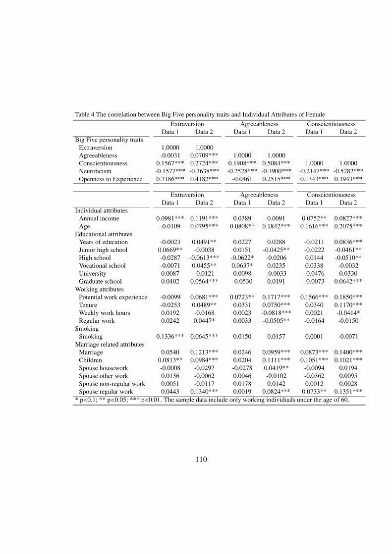
Table 4 The correlation between Big Five personality traits and Individual Attributes of FemaleExtraversion Agreeableness Conscientiousness
Data 1 Data 2 Data 1 Data 2 Data 1 Data 2Big Five personality traits
Extraversion 1.0000 1.0000Agreeableness -0.0031 0.0709*** 1.0000 1.0000Conscientiousness 0.1567*** 0.2724*** 0.1908*** 0.5084*** 1.0000 1.0000Neuroticism -0.1577*** -0.3638*** -0.2528*** -0.3900*** -0.2147*** -0.5282***Openness to Experience 0.3186*** 0.4182*** -0.0461 0.2515*** 0.1343*** 0.3943***
Extraversion Agreeableness ConscientiousnessData 1 Data 2 Data 1 Data 2 Data 1 Data 2
Individual attributesAnnual income 0.0981*** 0.1191*** 0.0389 0.0091 0.0752** 0.0827***Age -0.0109 0.0795*** 0.0808** 0.1842*** 0.1616*** 0.2075***
Educational attributesYears of education -0.0023 0.0491** 0.0227 0.0288 -0.0211 0.0836***Junior high school 0.0669** -0.0038 0.0151 -0.0425** -0.0222 -0.0461**High school -0.0287 -0.0613*** -0.0622* -0.0206 0.0144 -0.0510**Vocational school -0.0071 0.0455** 0.0637* 0.0235 0.0338 -0.0032University 0.0087 -0.0121 0.0098 -0.0033 -0.0476 0.0330Graduate school 0.0402 0.0564*** -0.0530 0.0191 -0.0073 0.0642***
Working attributesPotential work experience -0.0099 0.0681*** 0.0723** 0.1717*** 0.1566*** 0.1850***Tenure -0.0253 0.0489** 0.0331 0.0750*** 0.0340 0.1170***Weekly work hours 0.0192 -0.0168 0.0023 -0.0818*** 0.0021 -0.0414*Regular work 0.0242 0.0447* 0.0033 -0.0505** -0.0164 -0.0150
SmokingSmoking 0.1336*** 0.0645*** 0.0150 0.0157 0.0001 -0.0071
Marriage related attributesMarriage 0.0540 0.1213*** 0.0246 0.0959*** 0.0873*** 0.1400***Children 0.0813** 0.0984*** 0.0204 0.1111*** 0.1051*** 0.1021***Spouse housework -0.0008 -0.0297 -0.0278 0.0419** -0.0094 0.0194Spouse other work 0.0136 -0.0062 0.0046 -0.0102 -0.0362 0.0095Spouse non-regular work 0.0051 -0.0117 0.0178 0.0142 0.0012 0.0028Spouse regular work 0.0443 0.1340*** 0.0019 0.0824*** 0.0733** 0.1351***
* p<0.1; ** p<0.05; *** p<0.01. The sample data include only working individuals under the age of 60.
110

Table 4 The correlation between Big Five personality traits and IndividualAttributes of Female (Cont.)
Neuroticism Openness to ExperienceData 1 Data 2 Data 1 Data 2
Big Five personality traitsExtraversionAgreeablenessConscientiousnessNeuroticism 1.0000 1.0000Openness to Experience -0.0961*** -0.2489*** 1.0000 1.0000
Neuroticism Openness to ExperienceData 1 Data 2 Data 1 Data 2
Individual attributesAnnual income -0.1015*** -0.0960*** 0.0924*** 0.1035***Age -0.0902*** -0.2629*** -0.0421 0.0913***
Educational attributesYears of education -0.0156 -0.0677*** 0.0479 0.0891***Junior high school 0.0240 0.0393 0.0017 -0.0167High school -0.0069 0.0579*** -0.0553* -0.0681***Vocational school 0.0096 -0.0302 0.0380 0.0017University -0.0062 -0.0087 0.0131 0.0311Graduate school -0.0278 -0.0542** 0.0533 0.0792***
Working attributesPotential work experience -0.0824** -0.2407*** -0.0485 0.0729***Tenure -0.0693** -0.1275*** -0.0044 0.0559***Weekly work hours -0.0365 0.0513** 0.0572* 0.0007Regular work -0.0331 0.0482** 0.0496 0.0350
SmokingSmoking 0.0399 -0.0102 0.0040 0.0300
Marriage related attributesMarriage -0.0317 -0.1577*** -0.0200 -0.0197Children -0.0284 -0.1701*** -0.0351 -0.0519**Spouse housework -0.0220 -0.0236 -0.0213 -0.0299Spouse other work 0.0304 -0.0352* 0.0323 -0.0074Spouse non-regular work -0.0268 -0.0382* -0.0061 -0.0310Spouse regular work -0.0151 -0.1371*** -0.0161 -0.0009
* p<0.1; ** p<0.05; *** p<0.01.The sample data include only working individuals under the age of 60.
111
annual income, marriage, children, and spouse regular work. Appendix Table 4
is the estimation results of simple linear regression of each Big-Five personality
trait on annual income, years of education, smoking and marriage for females.
The results for the two datasets are similar in Table 4.
Concerning the relationship between the Big-Five personality traits and smok-
ing, relations are positive between Extraversion and smoking for both males and
females, but no statistically significant relationships are observed between other
personality traits and smoking. This indicates the Big-Five personality traits have
low potential for explaining the factors of unobservable individual heterogeneity.
On the other hand, the relationship between the Big-Five personality traits and
marriage-related attributes seems to be stronger than the relationship with smok-
ing. Almost all Big-Five personality traits have statistically significant positive
or negative correlations with marriage status, especially for males. Though there
is variability among spouse working status, the Big-Five personality traits are the
likely factors of unobservable individual heterogeneity when explaining wage dif-
ferences between married males who have full-time housewives and other males
in Chapter 3.
Through these results, it is obvious that the relationship between the Big-Five
personality traits and individual attributes seems to be different for Data 1 and 2.
This can be deemed to imply that the Big-Five personality traits in Data 1 repre-
sent a different personality from the Big-Five personality traits in Data 2. Next,
we focus on annual income and review how the differences in the two datasets ob-
served in the estimations of the income equation after controlling for other factors,
112

affect income.
4.4.2 Effect of the Big-Five personality traits on Annual Income
In accordance with the work of Lee and Ohtake (2014), we estimated the equa-
tion that respectively treats annual income as a dependent measure. In doing so,
we sought to compare the effects of Big-Five personality traits (derived from dif-
ferent inventories) on economic outcomes.
The estimation model is expressed as follows:
ln(Annual Incomei) = α + β1BFPTi + Xi β2 + vi
where Annual Incomei represents a median value of annual income categories;
BFPTi depicts Big-Five personality traits normalized and scaled to take values
between 0 and 1; Xi is a vector of individual attributes (e.g., individual educational
background, weekly working hours, potential years of work experience, tenure).
Because of mandatory retirement in Japan, income declines rapidly after 60 years
of age. As such, the sample data include only working individuals under the age
of 60. The random variable vi is an error term.
Table 5 summarizes the estimation results of the income equation.
Specifically, these results show the Big-Five personality traits except Agree-
ableness to be similar across the two datasets. Clear differences between the
datasets in terms of income emerge only with respect to Agreeableness. For the
pooled samples, there is a significant negative relationship between Agreeableness
113

Table 5 Results with IPWExplained Variable: Male FemaleLog Annual income Data 1 Data 2 Data 1 Data 2Extraversion 0.176 0.306 0.160 0.261
(0.091)* (0.073)*** (0.082)* (0.087)***Agreeableness 0.069 -0.075 0.024 -0.189
(0.122) (0.095) (0.128) (0.107)*Conscientiousness 0.343 0.477 0.220 0.025
(0.088)*** (0.092)*** (0.106)** (0.107)Neuroticism -0.220 -0.351 -0.181 -0.144
(0.113)* (0.089)*** (0.106)* (0.100)Openness to Experience -0.080 -0.169 0.018 0.171
(0.102) (0.079)** (0.106) (0.090)*High school 0.102 0.267 0.051 -0.028
(0.097) (0.070)*** (0.080) (0.115)Vocational school 0.158 0.285 0.214 0.029
(0.107) (0.072)*** (0.084)** (0.114)University 0.399 0.567 0.288 0.208
(0.099)*** (0.069)*** (0.091)*** (0.115)*Graduate school 0.621 0.827 0.521 0.345
(0.147)*** (0.073)*** (0.234)** (0.127)***Weekly working hours 0.004 0.009 0.019 0.018
(0.002)* (0.001)*** (0.002)*** (0.001)***Potential work experience 0.037 0.048 0.001 0.010
(0.010)*** (0.004)*** (0.009) (0.004)**(Potential work experience)2 -0.001 -0.001 -0.000 -0.000
(0.000)*** (0.000)*** (0.000) (0.000)***Tenure 0.032 0.031 0.029 0.033
(0.008)*** (0.004)*** (0.007)*** (0.005)***(Tenure)2 -0.000 -0.000 -0.000 -0.000
(0.000)* (0.000)** (0.000) (0.000)Constant term 4.684 4.324 4.156 4.337
(0.203)*** (0.128)*** (0.223)*** (0.160)***R2 0.35 0.39 0.41 0.40N 984 3,840 915 2,198* p<0.1; ** p<0.05; *** p<0.01. Standard error is noted in brackets.
114
and income for Data 2 respondents. The only significant effect is among Data 2 fe-
male respondents (and this relationship is only marginally significant). Regarding
other personality traits, the results show Extraversion and Conscientiousness to
be positively related to annual income and Neuroticism to be negatively related to
annual income. The effect of Openness to Experience among males and females
is opposite, negative for males and positive for females, and statistically insignif-
icantly in Data 1. Comparing the impact, the results show stronger positive or
negative effects in Data 2 than in Data 1 for males, whereas only Extraversion and
Openness to Experience have stronger effects in Data 2 for females.
These results suggest that there are differences between the two datasets in
terms of both the impacts and directions of the effects of the Big-Five personal-
ity traits on annual income. We found that the relationships between Agreeable-
ness and annual income differ across datasets.51 Given these findings, a question
emerges: what is driving these differences?
We believe there are two possible reasons the databases differ along the lines
described above. First, it is possible that some of the items in the Big-Five person-
ality inventory somehow may be problematic, thereby causing variance across the
two datasets. Second, our method of quantifying the Big-Five personality traits
from the items in the index may have been problematic. In the following sections,
we explore these possibilities. First, we estimate the direct effects of each individ-
ual item on the outcome variables to determine whether they were problematic.
51 Appendix Table 5 shows the estimation results using another IPW estimated along the linesof sex, age, educational background, income level, weekly working hours, and occupation andindustry information. The results are similar to those presented in Table 5.
115

Second, rather than use the Big-Five scores obtained by adding up individual item
scores, we use the first principal component obtained via a principal component
analysis to identify the leading causes of the differences between the two datasets.
4.4.3 Item Effects
One source of variation in the effects intrinsic to each dataset is the possible
differences in the effects of individual items on outcome measures within the two
datasets. As described in Footnote 48, measurement of the Big-Five personality
traits involved the use of forward- and reverse-coded items in both datasets. For
example, two items formed the Extraversion index in Data 1. While one of these
items was straightforward and directly related to Extraversion (i.e., “Extraverted,
Enthusiastic”), the other was oppositely related to Extraversion (i.e., “Reserved,
Quiet”) and required reverse-coding. Similar issues characterized Data 2; mea-
surement of Extraversion in Data 2 involved five straightforward questions (“I am
talkative,” “I am energetic,” “I am quite enthusiastic,” “I am aggressive,” and “I
am outgoing”) and three reverse-coded questions (“I am conservative,” “I am a
quiet person,” and “I am bashful”).
To calculate the overall scores for each of the Big-Five personality traits, we
simply took their unweighted average. If every item accurately captured the per-
sonal traits to which they were geared, items in both datasets should have exerted
similar effects on corresponding outcomes. Different effect sizes for similar items
suggest that the items were not measuring the same construct, and therefore cap-
116
tured different aspects of personalities. This, in turn, could yield different effects
of the Big-Five on the aforementioned outcomes across the two datasets.
Table 6 summarizes the results of the analyses geared towards testing these
possibilities. In each part, values in the first row indicate the results from Table 5.
Sentences wish asterisk indicate that the items were reverse-coded.
117

Tabl
e6
Res
ults
ofE
ach
Inve
ntor
yw
ithIP
WD
ata
1D
ata
2O
utco
me
vari
able
:Ann
uali
ncom
eM
ale
Fem
ale
Out
com
eva
riab
le:A
nnua
linc
ome
Mal
eFe
mal
e1.
Ext
rave
rsio
nE
xtra
vers
ion
(Tab
le5)
0.03
20.
028
Ext
rave
rsio
n(T
able
5)0.
023
0.02
0(0
.016
)**
(0.0
14)*
*(0
.006
)***
(0.0
07)*
**E
xtra
vert
ed,E
nthu
sias
tic-0
.049
0.01
7Ia
mta
lkat
ive.
-0.0
66-0
.035
(0.1
05)
(0.0
89)
(0.0
46)
(0.0
61)
Res
erve
d,Q
uiet
*0.
220
0.15
7Ia
mco
nser
vativ
e.*
0.05
50.
140
(0.1
04)*
*(0
.097
)(0
.055
)(0
.073
)*Ia
men
erge
tic.
0.04
80.
010
(0.0
62)
(0.0
74)
Iam
quite
enth
usia
stic
.-0
.031
0.01
3(0
.060
)(0
.074
)Ia
ma
quie
tper
son.
*0.
102
0.05
2(0
.058
)*(0
.068
)Ia
mag
gres
sive
.0.
142
0.01
4(0
.058
)**
(0.0
71)
Iam
bash
ful.
*-0
.059
0.05
8(0
.057
)(0
.068
)Ia
mou
tgoi
ng.
0.08
1-0
.017
(0.0
55)
(0.0
69)
R2
0.36
0.41
R2
0.41
0.42
N98
491
5N
3,84
02,
198
*p<
0.1;
**p<
0.05
;***
p<0.
01.S
tand
ard
erro
ris
note
din
brac
kets
.Fo
rall
estim
atio
ns,e
duca
tiona
lbac
kgro
und,
wee
kly
wor
king
hour
s,ye
ars
ofw
ork
expe
rien
cean
dits
squa
re,a
ndte
nure
and
itssq
uare
are
cont
rolle
d.
118

T abl
e6
Res
ults
ofE
ach
Inve
ntor
yw
ithIP
W(C
ont.)
Dat
a1
Dat
a2
Out
com
eva
riab
le:A
nnua
linc
ome
Mal
eFe
mal
eO
utco
me
vari
able
:Ann
uali
ncom
eM
ale
Fem
ale
2.A
gree
able
ness
Agr
eeab
lene
ss(T
able
5)0.
009
0.00
2A
gree
able
ness
(Tab
le5)
-0.0
05-0
.010
(0.0
17)
(0.0
18)
(0.0
06)
(0.0
07)
Cri
tical
,Qua
rrel
som
e*
0.05
80.
099
Ifind
faul
tsin
othe
rs.*
-0.0
020.
024
(0.0
96)
(0.1
04)
(0.0
49)
(0.0
59)
Sym
path
etic
,War
m0.
088
-0.0
76Ia
mki
ndto
othe
rs.
0.00
8-0
.030
(0.1
13)
(0.1
29)
(0.0
62)
(0.0
83)
Iten
dto
argu
ew
ithot
hers
.*0.
071
-0.0
74(0
.050
)(0
.065
)Ih
ave
afo
rgiv
ing
natu
re.
0.04
90.
016
(0.0
46)
(0.0
56)
Iam
trus
twor
thy.
-0.0
710.
130
(0.0
72)
(0.0
81)
Iam
stuc
kup
.*-0
.070
-0.1
49(0
.058
)(0
.072
)**
Iam
thou
ghtf
ulan
dki
nd.
-0.1
570.
039
(0.0
69)*
*(0
.095
)Ia
mru
deto
othe
rs.*
0.04
80.
036
(0.0
55)
(0.0
61)
Ilik
eto
coop
erat
ew
ithot
hers
.0.
028
-0.0
15(0
.064
)(0
.069
)
R2
0.36
0.41
R2
0.41
0.42
N98
491
5N
3,84
02,
198
*p<
0.1;
**p<
0.05
;***
p<0.
01.S
tand
ard
erro
ris
note
din
brac
kets
.Fo
rall
estim
atio
ns,e
duca
tiona
lbac
kgro
und,
wee
kly
wor
king
hour
s,ye
ars
ofw
ork
expe
rien
cean
dits
squa
re,a
ndte
nure
and
itssq
uare
are
cont
rolle
d.
119

Tabl
e6
Res
ults
ofE
ach
Inve
ntor
yw
ithIP
W(C
ont.)
Dat
a1
Dat
a2
Out
com
eva
riab
le:A
nnua
linc
ome
Mal
eFe
mal
eO
utco
me
vari
able
:Ann
uali
ncom
eM
ale
Fem
ale
3.C
onsc
ient
ious
ness
Con
scie
ntio
usne
ss(T
able
5)0.
053
0.03
4C
onsc
ient
ious
ness
(Tab
le5)
0.03
50.
002
(0.0
14)*
**(0
.016
)**
(0.0
06)*
**(0
.007
)D
epen
dabl
e,Se
lf-D
isci
plin
ed0.
213
0.12
1Ia
ma
perf
ectio
nist
whe
nit
com
esto
wor
k.-0
.028
-0.1
35(0
.091
)**
(0.1
10)
(0.0
53)
(0.0
65)*
*D
isor
gani
zed,
Car
eles
s*
0.14
80.
098
Iam
abi
tcar
eles
s.*
0.05
0-0
.065
(0.0
79)*
(0.0
80)
(0.0
52)
(0.0
61)
Iam
atr
uste
dw
orke
r.0.
246
0.12
4(0
.065
)***
(0.0
82)
Iam
emot
iona
llyin
secu
re.*
0.00
30.
031
(0.0
57)
(0.0
70)
Iten
dto
bela
zy.*
0.05
1-0
.020
(0.0
51)
(0.0
58)
Icar
ryou
tmy
wor
kun
tilit
isco
mpl
eted
.0.
010
0.03
1(0
.064
)(0
.077
)Id
ealw
ithm
atte
rseffi
cien
tly.
0.02
00.
029
(0.0
59)
(0.0
70)
Icar
ryou
tmy
plan
s.0.
107
-0.0
57(0
.055
)*(0
.065
)Ih
ave
prob
lem
sin
conc
entr
atin
g.*
-0.0
82-0
.017
(0.0
54)
(0.0
65)
R2
0.36
0.41
R2
0.41
0.42
N98
491
5N
3,84
02,
198
*p<
0.1;
**p<
0.05
;***
p<0.
01.S
tand
ard
erro
ris
note
din
brac
kets
.Fo
rall
estim
atio
ns,e
duca
tiona
lbac
kgro
und,
wee
kly
wor
king
hour
s,ye
ars
ofw
ork
expe
rien
cean
dits
squa
re,a
ndte
nure
and
itssq
uare
are
cont
rolle
d.
120

Tabl
e6
Res
ults
ofE
ach
Inve
ntor
yw
ithIP
W(C
ont.)
Dat
a1
Dat
a2
Out
com
eva
riab
le:A
nnua
linc
ome
Mal
eFe
mal
eO
utco
me
vari
able
:Ann
uali
ncom
eM
ale
Fem
ale
4.N
euro
ticis
mN
euro
ticis
m(T
able
5)-0
.032
-0.0
28N
euro
ticis
m(T
able
5)-0
.028
-0.0
09(0
.017
)*(0
.016
)*(0
.007
)***
(0.0
07)
Anx
ious
,Eas
ilyup
set
-0.1
25-0
.052
Ilac
ken
ergy
.-0
.059
0.02
7(0
.091
)(0
.095
)(0
.054
)(0
.067
)C
alm
,Em
otio
nally
stab
le*
-0.0
77-0
.114
Iam
easy
goin
g.*
-0.0
45-0
.091
(0.1
07)
(0.1
06)
(0.0
55)
(0.0
64)
Ibec
ome
nerv
ous
easi
ly.
-0.0
15-0
.086
(0.0
54)
(0.0
62)
Iwor
ryab
outm
any
thin
gs.
0.01
2-0
.105
(0.0
50)
(0.0
59)*
Iam
emot
iona
llyse
cure
.*-0
.140
0.08
7(0
.061
)**
(0.0
76)
Iam
moo
dy.
0.00
50.
023
(0.0
51)
(0.0
56)
Irem
ain
calm
even
inst
ress
fuls
ituat
ions
.*-0
.103
-0.0
63(0
.058
)*(0
.060
)Ia
ma
nerv
ous
pers
on.
-0.1
090.
103
(0.0
50)*
*(0
.056
)*
R2
0.36
0.41
R2
0.41
0.42
N98
491
5N
3,84
02,
198
*p<
0.1;
**p<
0.05
;***
p<0.
01.S
tand
ard
erro
ris
note
din
brac
kets
.Fo
rall
estim
atio
ns,e
duca
tiona
lbac
kgro
und,
wee
kly
wor
king
hour
s,ye
ars
ofw
ork
expe
rien
cean
dits
squa
re,a
ndte
nure
and
itssq
uare
are
cont
rolle
d.
121
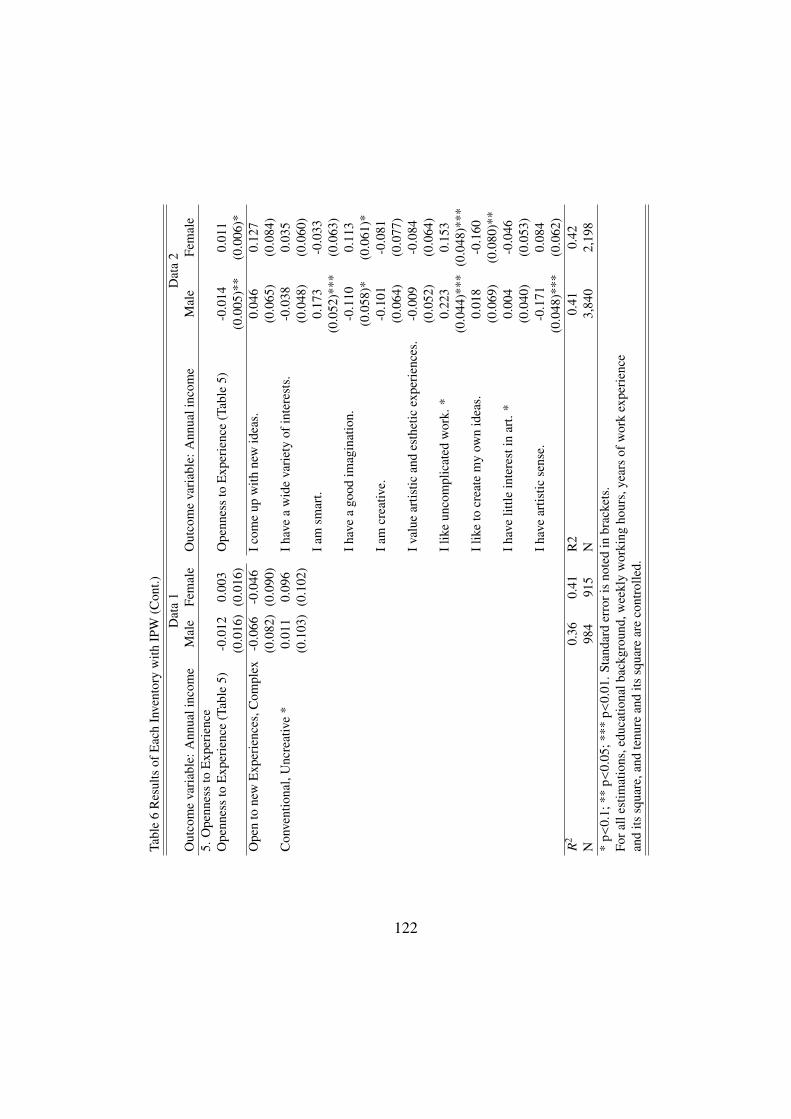
T abl
e6
Res
ults
ofE
ach
Inve
ntor
yw
ithIP
W(C
ont.)
Dat
a1
Dat
a2
Out
com
eva
riab
le:A
nnua
linc
ome
Mal
eFe
mal
eO
utco
me
vari
able
:Ann
uali
ncom
eM
ale
Fem
ale
5.O
penn
ess
toE
xper
ienc
eO
penn
ess
toE
xper
ienc
e(T
able
5)-0
.012
0.00
3O
penn
ess
toE
xper
ienc
e(T
able
5)-0
.014
0.01
1(0
.016
)(0
.016
)(0
.005
)**
(0.0
06)*
Ope
nto
new
Exp
erie
nces
,Com
plex
-0.0
66-0
.046
Icom
eup
with
new
idea
s.0.
046
0.12
7(0
.082
)(0
.090
)(0
.065
)(0
.084
)C
onve
ntio
nal,
Unc
reat
ive
*0.
011
0.09
6Ih
ave
aw
ide
vari
ety
ofin
tere
sts.
-0.0
380.
035
(0.1
03)
(0.1
02)
(0.0
48)
(0.0
60)
Iam
smar
t.0.
173
-0.0
33(0
.052
)***
(0.0
63)
Ihav
ea
good
imag
inat
ion.
-0.1
100.
113
(0.0
58)*
(0.0
61)*
Iam
crea
tive.
-0.1
01-0
.081
(0.0
64)
(0.0
77)
Ival
uear
tistic
and
esth
etic
expe
rien
ces.
-0.0
09-0
.084
(0.0
52)
(0.0
64)
Ilik
eun
com
plic
ated
wor
k.*
0.22
30.
153
(0.0
44)*
**(0
.048
)***
Ilik
eto
crea
tem
yow
nid
eas.
0.01
8-0
.160
(0.0
69)
(0.0
80)*
*Ih
ave
little
inte
rest
inar
t.*
0.00
4-0
.046
(0.0
40)
(0.0
53)
Ihav
ear
tistic
sens
e.-0
.171
0.08
4(0
.048
)***
(0.0
62)
R2
0.36
0.41
R2
0.41
0.42
N98
491
5N
3,84
02,
198
*p<
0.1;
**p<
0.05
;***
p<0.
01.S
tand
ard
erro
ris
note
din
brac
kets
.Fo
rall
estim
atio
ns,e
duca
tiona
lbac
kgro
und,
wee
kly
wor
king
hour
s,ye
ars
ofw
ork
expe
rien
cean
dits
squa
re,a
ndte
nure
and
itssq
uare
are
cont
rolle
d.
122

As outlined in the previous section, the two datasets differed in terms of some
of the relationships between the Big-Five traits and salient outcomes. For instance,
the two datasets differed in terms of the relationship between Agreeableness and
income.
In Table 6, the individual items geared towards measuring Agreeableness pro-
vide some insight into the construct. Among Data 1 respondents, all items were
non-significant. There is a similar pattern among Data 2 respondents, where most
effects are again non-significant. Only “I am stuck up” and “I am thoughtful and
kind” have significant effects for males and females. Though non-significant, it
is important to note that several items (e.g., “I tend to argue with others,” “I am
trustworthy,” “I like to cooperate with others”) have opposite signs than expected.
Despite the ubiquity of the unexpected signs of the estimates, negative estimates
seem to be more predictive of Agreeableness than positive estimates relative to
the values listed in Data 1. These results suggest that Data 1 more effectively
highlights the positive effects of these items on Agreeableness, and Data 2 more
effectively captures the negative effects. This is likely due to differences in the
items that comprise the two questionnaires.
These results suggest that variations in how the items are expressed induce
greater deviations in the estimates for several personality traits in Data 2 relative
to Data 1. Although Data 1 uses fewer items to measure personality traits than
Data 2, each item in the former may be interpreted as having two meanings (e.g.,
“Critical” vs. “Quarrelsome”). This type of question may capture personality
traits more accurately than the broader questions used for Data 2. Stated simply,
123
questions in Data 1 may capture personality more specifically and directly than
questions in Data 2. Consider, for example, if a Data 1 respondent scored high
on the “Critical, Quarrelsome” item. This respondent may have been indicating
that he/she is more critical and quarrelsome rather than critical or quarrelsome. In
contrast, the Data 2 item “I tend to argue with others” may appeal to those who are
argumentative, but not those who are critical. In sum, questionnaire items used to
compile Data 2 are of a greater variety than those in Data 1, suggesting that the
items in the former capture more abstract personality traits than the latter.
4.4.4 Principal Component Analysis
The other possible genesis of differences between the two datasets related to
the effects of the Big-Five personality traits concerns the method we used to quan-
tify those traits. In short, it is possible that simply adding (or averaging) responses
to individual items is not a useful approach. As mentioned in Footnote 48, to quan-
tify the Big-Five scores, we simply took the post-normalization mean of the scores
from the individual questions. In this section, we determine the principal compo-
nent from each group of items related to the respective personality traits. We then
use this principal component value as the respondent’s score on that personality
trait.
In Appendix Table 6, the values with asterisk show the contribution ratio for
the first principal component. In Data 1, the first principal components accounted
for between 66% and 80% of the variance in the Big-Five personality traits. This
124

ratio is much smaller in Data 2; in this dataset, the first principal components
accounted for between 34% and 42% of the variance in the Big-Five personality
traits. Although the contributions of the first principal components is less pro-
nounced in Data 2 than Data 1, it is nonetheless valid to use only the first principal
components for Data 2, due to observable differences between the first and second
principal components.
Table 7 summarizes the results of the principal components analyses in rela-
tion to income.
The results outlined in Table 7 show the same tendencies as those in Table
5. There was a positive effect between Extraversion and Conscientiousness and
annual income and a negative relationship between Neuroticism and annual in-
come. Results related to Openness to Experience were similar to those in Table 5
(though smaller in magnitude). Taken together, these results indicate that differ-
ences between the two datasets with respect to Agreeableness are robust when the
personality traits are determined via a principal components analysis. However,
the differences become much smaller than in Table 5, indicating that the Big-Five
personality traits in Data 2 capture a wider breadth of the personality than in Data
1, and thus supports our discussion in Section 4.4.3.
Although the estimates reported in Table 7 are smaller than those reported in
Table 5, the directions of all effects are identical. Moreover, nearly all effects that
were statistically significant in Table 5 emerged as significant in Table 7.
In sum, the estimation results that used the first principal components as in-
dicators of Big-Five personality traits were similar to results that emerged from
125

Table 7 Results of First Principle Component with IPWExplained Variable: Male FemaleLog Annual income Data 1 Data 2 Data 1 Data 2Extraversion 0.032 0.023 0.028 0.020
(0.016)** (0.006)*** (0.014)** (0.007)***Agreeableness 0.009 -0.005 0.002 -0.010
(0.017) (0.006) (0.018) (0.007)Conscientiousness 0.053 0.035 0.034 0.002
(0.014)*** (0.006)*** (0.016)** (0.007)Neuroticism -0.032 -0.028 -0.028 -0.009
(0.017)* (0.007)*** (0.016)* (0.007)Openness to Experience -0.012 -0.014 0.003 0.011
(0.016) (0.005)** (0.016) (0.006)*High school 0.102 0.269 0.052 -0.029
(0.097) (0.070)*** (0.080) (0.115)Vocational school 0.158 0.286 0.215 0.029
(0.107) (0.072)*** (0.084)** (0.114)University 0.399 0.568 0.289 0.209
(0.099)*** (0.069)*** (0.091)*** (0.115)*Graduate school 0.621 0.829 0.521 0.346
(0.147)*** (0.073)*** (0.234)** (0.127)***Weekly working hours 0.004 0.009 0.019 0.018
(0.002)* (0.001)*** (0.002)*** (0.001)***Potential work experience 0.037 0.048 0.001 0.010
(0.010)*** (0.004)*** (0.009) (0.004)**(Potential work experience)2 -0.001 -0.001 -0.000 -0.000
(0.000)*** (0.000)*** (0.000) (0.000)***Tenure 0.032 0.031 0.029 0.033
(0.008)*** (0.004)*** (0.007)*** (0.005)***(Tenure)2 -0.000 -0.000 -0.000 -0.000
(0.000)* (0.000)** (0.000) (0.000)Constant term 4.848 4.423 4.285 4.366
(0.181)*** (0.081)*** (0.151)*** (0.123)***R2 0.35 0.39 0.41 0.40N 984 3,840 915 2,198* p<0.1; ** p<0.05; *** p<0.01. Standard error is noted in brackets.
126

using averaged scores. This lends credence to the computation of the Big-Five
scores from indices (consistent with past research). This finding leads us to be-
lieve that few (if any) of the differences across the datasets are attributable to
individual items in the Big-Five inventory.
4.5 Conclusion
In this chapter, we have evaluated two questionnaires in their respective capac-
ities to measure the effect of the Big-Five personality traits on economic outcome
(income). The first questionnaire was a 10-item inventory developed by Gosling
et al. (2003), and the second was a pervasively used 44-item inventory. To control
for distribution differences across the two datasets produced by the administration
of these two questionnaires, we used inverse probability weighting to estimate
equations.
The results showed that the relationships between Extraversion, Conscien-
tiousness, Neuroticism, and Openness to Experience and the outcome variables
did not differ between the 10- and 44-item indices. In contrast, the relationship
between Agreeableness and income was slightly different across the two datasets.
To determine the source of this difference, we (a) calculated the effect of each item
on income, and (b) identified the first principal components as proxies for the Big-
Five personality traits. The results indicate that the differences between the two
datasets with regard to the relationships between Agreeableness and income may
derive from the ways in which the individual items are worded (and therefore, the
127

constructs they capture). Furthermore, our results show that the use of the first
principal components is a viable method for estimating the relationships between
the Big-Five and the outcome variables.
Through this chapter, we have shown that short questionnaires may be useful
for saving time, as they yield the same results as longer questionnaires, but only
for some personality traits under certain conditions. When using short measure-
ment instruments in empirical economic research, it is important to interpret the
findings carefully, especially those related to Agreeableness.
128
References[1] Benet-Martinez, V. and O. P. John (1998) “Los Cinco Grandes across Cul-
tures and Ethnic Groups: Multitrait Method Analyses of the Big Five inSpanish and English.” Journal of Personality and Social Psychology. 75 (3),729-750.
[2] Bowls, S., H. Gintis, and M. Osborne (2001) “The Determinants of Earn-ings: A Behavioral Approach.” Journal of Economic Literature. 39 (4),1137-1176.
[3] Costa P. T. Jr., and R. R. McCrae (1991) “Facet Scales for Agreeablenessand Conscientiousness: A Revision of the NEO Personality Inventory.” Per-sonality and Individual Differences. 12 (9), 887-898.
[4] Costa P. T. Jr., and R. R. McCrae (1992) Revised NEO Personality Inven-tory (NEO-PI-R) and NEO Five-Factor Inventory (NEO-FFI) professionalmanual. Odessa, FL: Psychological Assessment Resources.
[5] Fletcher, J. M. (2013) “The Effects of Personality Traits on Adult LaborMarket Outcomes: Evidence from Siblings.” Journal of Economic Behavior& Organization. 89, 122-135.
[6] Goldberg, L.R. (1992) “The Development of Markers for the Big-Five FactorStructure.” Psychological Assessment. 4 (1), 26-42.
[7] Gosling, S. D., P. J. Rentfrow, and W. B. Swann Jr. (2003) “A Very BriefMeasure of the Big-Five Personality Domains.” Journal of Research in Per-sonality. 37, 504-528.
[8] Heckman, J. J. (2000) “Policies to Foster Human Capital.” Research in Eco-nomics. 54 (1), 3-56.
[9] Heckman, J. J. and Y. Rubinstein (2001) “The Importance of NoncognitiveSkills: Lessons from the GED Testing Program.” American Economic Re-view. 91 (2), 145-149.
[10] Heckman, J. J., J. Stixrud, and S. Urzua (2006) “The Effects of Cognitive andNoncognitive Abilities on Labor Market Outcomes and Social Behavior.”Journal of Labour Economics. 24 (3), 411-482.
129

[11] Heineck, G., and S. Anger (2010) “The Returns to Cognitive Abilities andPersonality Traits in Germany.” Labour Economics. 17, 535-546.
[12] John, O. P. and S. Srivastava (1999) “The Big-Five Trait Taxonomy; History,Measurement, and Theoretical Perspectives.” L. A. Pervin and O. P. John(Eds.), Handbook of Personality: Theory and Research, 2, pp. 102-138, NewYork: Guiford Press.
[13] Lee, S. Y., and F. Ohtake (2014) “The Effects of Personality Traits and Be-havioral Characteristics on Schooling, Earnings, and Career Promotion.” RI-ETI Discussion Paper: 14-E-023.
[14] Mueller, G., and E. Plug (2006) “Estimating the Effect of Personality onMale and Female Earnings.” Industrial and Labor Relations Review. 60 (1),3-22.
[15] Nyhous, E. K., and E. Pons (2005) “The Effects of Personality on Earnings.”Journal of Economic Psychology. 26, 363-384.
[16] Osborne-Groves, M. (2005) “How Important is Your Personality? LaborMarket Returns to Personality for Women in the US and UK.” Journal ofEconomic Psychology. 26, 827-841.
[17] Wooldridge, J. M. (2005) “Simple Solutions to the Initial Conditions Prob-lem in Dynamic, Nonlinear Panel-Data Models with Unobserved Hetero-geneity.” Journal of Applied Econometrics. 20, 39-54.
130
5 Chapter 5 Conclusion
In this thesis, we used three sets of Japanese panel data to discuss the factors
affecting wage determination. We found that labor market earnings are deter-
mined by not only years of schooling and work experience but also gender, race,
region, and other observable and unobservable individual attributes. This thesis
also accounted for behavioral factors such as smoking and life events such as
intra-household specialization to identify factors contributing to wage disparities.
In Chapter 2, we use Japanese panel data (KHPS) to verify the hypothesis
that smoking behavior reduced wage levels. In the analyses, we controlled for
time-invariant individual heterogeneity, which previous studies failed to capture
using two-year panel data and cross-sectional data. In addition, we examined IV
estimations to control for time-variant individual heterogeneity and conducted ro-
bustness checks. The chapter also proved that wage differences can be attributed
to individual unobservable heterogeneity, not smoking behavior. However, unde-
niably, smoking negatively affects labor productivity through health damages and
causes changes in the wage level in the long run.
In Chapter 3, we applied the intra-household specialization hypothesis to iden-
tify the factors underpinning observed wage differences on the basis of marital
status for Japanese men. Using Japanese panel data, we found that unobservable
individual heterogeneity contributed to the wage gap based on males’ marital sta-
tus. Although we did not find clear evidence supporting the intra-household spe-
cialization hypothesis, the wage disparity between married and unmarried males
131

was obvious, thus indicating that intra-household specialization is not a factor
determining wage in Japan. We suspect other factors such as personality traits,
environment factors, and cultural characteristics lead to wage disparities based on
marital status.
In Chapter 4, we focus on the Big-Five personality traits and compare the
effects on economic outcomes using two types of questionnaires. Data 1 is ex-
amined using the 10-item questionnaire, as developed by Gosling et al. (2003),
while Data 2 applied the widely used 44-item questionnaire. To control for dis-
tribution differences among the two datasets, we estimate equations adjusted by
inverse probability weighting. One of the main findings of our analysis is that
short questions save time for researchers and respondents and have a consistent
effect on economic outcomes in comparison to the time-consuming yet widely
used 44-item questionnaire; this, however, applies to selected personality traits,
not all. When using short questions for economic empirical researches, it is im-
perative to pay careful attention to the interpretation of the results, especially in
the case of Agreeableness.
Finally, future works should consider examining the relationship between wages
and smoking, marriage, and individual unobservable individual. It is also neces-
sary to use long-term panel data to verify the mechanisms underlying wage deter-
mination in Japan.
132

A Appendix Tables
[Chapter 3 Men’s Wages and Intra-household Specialization]
Appendix Table 1..........................................................................................134
Appendix Table 2..........................................................................................136
Appendix Table 3..........................................................................................138
Appendix Table 4..........................................................................................140
[Chapter 4 Variation in the Effects of the Big-Five Personality Traits; The 10-
Item Scale versus the 44-Item Scale]
Appendix Table 1..........................................................................................142
Appendix Table 2..........................................................................................144
Appendix Table 3..........................................................................................145
Appendix Table 4..........................................................................................147
Appendix Table 5..........................................................................................149
133
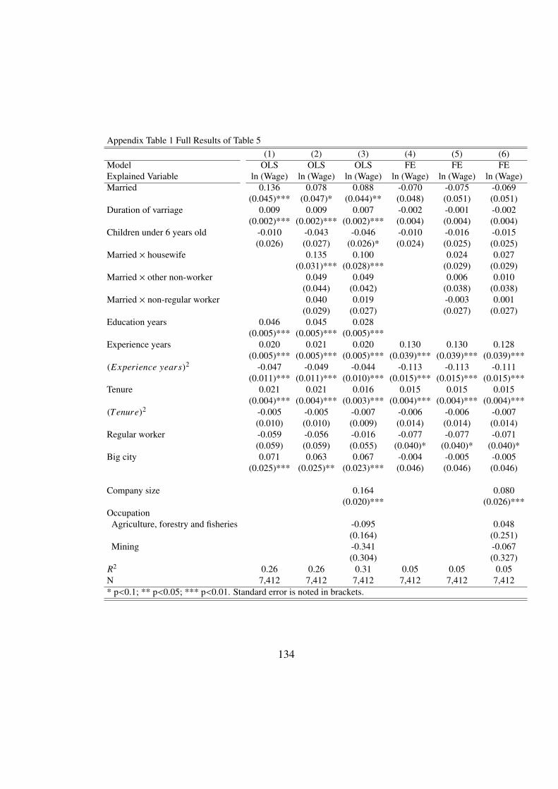
Appendix Table 1 Full Results of Table 5(1) (2) (3) (4) (5) (6)
Model OLS OLS OLS FE FE FEExplained Variable ln (Wage) ln (Wage) ln (Wage) ln (Wage) ln (Wage) ln (Wage)Married 0.136 0.078 0.088 -0.070 -0.075 -0.069
(0.045)*** (0.047)* (0.044)** (0.048) (0.051) (0.051)Duration of varriage 0.009 0.009 0.007 -0.002 -0.001 -0.002
(0.002)*** (0.002)*** (0.002)*** (0.004) (0.004) (0.004)Children under 6 years old -0.010 -0.043 -0.046 -0.010 -0.016 -0.015
(0.026) (0.027) (0.026)* (0.024) (0.025) (0.025)Married × housewife 0.135 0.100 0.024 0.027
(0.031)*** (0.028)*** (0.029) (0.029)Married × other non-worker 0.049 0.049 0.006 0.010
(0.044) (0.042) (0.038) (0.038)Married × non-regular worker 0.040 0.019 -0.003 0.001
(0.029) (0.027) (0.027) (0.027)Education years 0.046 0.045 0.028
(0.005)*** (0.005)*** (0.005)***Experience years 0.020 0.021 0.020 0.130 0.130 0.128
(0.005)*** (0.005)*** (0.005)*** (0.039)*** (0.039)*** (0.039)***(Experience years)2 -0.047 -0.049 -0.044 -0.113 -0.113 -0.111
(0.011)*** (0.011)*** (0.010)*** (0.015)*** (0.015)*** (0.015)***Tenure 0.021 0.021 0.016 0.015 0.015 0.015
(0.004)*** (0.004)*** (0.003)*** (0.004)*** (0.004)*** (0.004)***(Tenure)2 -0.005 -0.005 -0.007 -0.006 -0.006 -0.007
(0.010) (0.010) (0.009) (0.014) (0.014) (0.014)Regular worker -0.059 -0.056 -0.016 -0.077 -0.077 -0.071
(0.059) (0.059) (0.055) (0.040)* (0.040)* (0.040)*Big city 0.071 0.063 0.067 -0.004 -0.005 -0.005
(0.025)*** (0.025)** (0.023)*** (0.046) (0.046) (0.046)
Company size 0.164 0.080(0.020)*** (0.026)***
OccupationAgriculture, forestry and fisheries -0.095 0.048
(0.164) (0.251)Mining -0.341 -0.067
(0.304) (0.327)R2 0.26 0.26 0.31 0.05 0.05 0.05N 7,412 7,412 7,412 7,412 7,412 7,412* p<0.1; ** p<0.05; *** p<0.01. Standard error is noted in brackets.
134

Appendix Table 1 Full Results of Table 5 (Cont.)(1) (2) (3) (4) (5) (6)
Model OLS OLS OLS FE FE FEExplained Variable ln (Wage) ln (Wage) ln (Wage) ln (Wage) ln (Wage) ln (Wage)OccupationSales 0.026 -0.050
(0.075) (0.049)Services -0.164 -0.048
(0.082)** (0.054)Management works 0.397 0.082
(0.077)*** (0.048)*Clercal works 0.180 0.035
(0.072)** (0.046)Transportation and telecom works -0.022 -0.000
(0.078) (0.058)Field works 0.098 0.077
(0.071) (0.045)*Information technology engineer 0.254 -0.060
(0.083)*** (0.070)Professional and technique works 0.238 0.039
(0.075)*** (0.045)Security 0.203 0.082
(0.084)** (0.100)
Year Dummy: 2005 0.033 0.035 0.067 -0.039 -0.038 -0.031(0.057) (0.056) (0.053) (0.054) (0.054) (0.054)
Year Dummy: 2006 -0.004 -0.002 0.022 -0.133 -0.132 -0.121(0.058) (0.057) (0.054) (0.084) (0.084) (0.084)
Year Dummy: 2007 0.014 0.016 0.041 -0.175 -0.174 -0.166(0.058) (0.058) (0.055) (0.118) (0.118) (0.118)
Year Dummy: 2008 0.011 0.015 0.035 -0.244 -0.243 -0.234(0.056) (0.055) (0.052) (0.154) (0.154) (0.154)
Year Dummy: 2009 0.046 0.050 0.074 -0.275 -0.273 -0.264(0.056) (0.056) (0.052) (0.190) (0.190) (0.190)
Year Dummy: 2010 -0.015 -0.012 0.014 -0.397 -0.395 -0.383(0.057) (0.057) (0.053) (0.226)* (0.226)* (0.227)*
Year Dummy: 2011 0.011 0.012 0.036 -0.438 -0.437 -0.425(0.059) (0.058) (0.055) (0.263)* (0.263)* (0.263)
Year Dummy: 2012 0.005 0.006 0.031 -0.509 -0.508 -0.493(0.058) (0.058) (0.054) (0.300)* (0.300)* (0.300)
Constant term 6.306 6.311 6.424 5.470 5.468 5.441(0.105)*** (0.104)*** (0.119)*** (0.734)*** (0.734)*** (0.736)***
R2 0.26 0.26 0.31 0.05 0.05 0.05N 7,412 7,412 7,412 7,412 7,412 7,412* p<0.1; ** p<0.05; *** p<0.01. Standard error is noted in brackets.
135

Appendix Table 2 Full Results of Table 8(8) (9) (10)
Model FD FD FDExplained Variable ln (Wage) ln (Wage) ln (Wage)Married -0.069 -0.055 -0.048
(0.078) (0.082) (0.083)Duration of marriage 0.004 0.005 0.005
(0.005) (0.005) (0.005)Children under 6 years old -0.010 -0.015 -0.014
(0.040) (0.041) (0.041)Married × housewife -0.013 -0.009
(0.040) (0.040)Married × other non-worker 0.021 0.027
(0.046) (0.046)Married × regular worker -0.043 -0.039
(0.034) (0.034)Education years 0.354 0.356 0.350
(0.173)** (0.173)** (0.189)*Experience years 0.267 0.270 0.271
(0.091)*** (0.090)*** (0.090)***(Experience years)2 -0.083 -0.085 -0.084
(0.029)*** (0.029)*** (0.029)***Tenure 0.021 0.021 0.020
(0.009)** (0.009)** (0.009)**(Tenure)2 -0.038 -0.037 -0.035
(0.028) (0.028) (0.027)Regular worker -0.059 -0.059 -0.051
(0.072) (0.072) (0.071)Big city -0.068 -0.070 -0.076
(0.079) (0.079) (0.078)
Company size 0.080(0.035)**
Occupation:Agriculture, forestry and fisheries 0.049
(0.185)Mining -0.280
(0.213)Sales -0.010
(0.079)Services -0.069
(0.085)R2 0.01 0.01 0.02N 5,070 5,070 5,070* p<0.1; ** p<0.05; *** p<0.01. Standard error is noted in brackets.
136

Appendix Table 2 Full Results of Table 8 (Cont.)(8) (9) (10)
Model FD FD FDExplained Variable ln (Wage) ln (Wage) ln (Wage)Occupation:Management works 0.074
(0.070)Clercal works 0.049
(0.070)Transportation and telecom works -0.015
(0.081)Field works 0.059
(0.073)Information technology engineer -0.059
(0.091)Professional and technique works 0.050
(0.068)Security 0.110
(0.106)
Year Dummy: 2005 -0.157 -0.157 -0.154(0.123) (0.123) (0.123)
Year Dummy: 2006 -0.387 -0.389 -0.393(0.206)* (0.205)* (0.206)*
Year Dummy: 2007 -0.565 -0.569 -0.580(0.294)* (0.293)* (0.293)**
Year Dummy: 2008 -0.756 -0.761 -0.778(0.378)** (0.377)** (0.376)**
Year Dummy: 2009 -0.913 -0.920 -0.945(0.464)** (0.463)** (0.462)**
Year Dummy: 2010 -1.154 -1.162 -1.192(0.551)** (0.549)** (0.548)**
Year Dummy: 2011 -1.312 -1.321 -1.360(0.638)** (0.635)** (0.634)**
Constant -0.028 -0.029 -0.023(0.029) (0.029) (0.028)
R2 0.01 0.01 0.02N 5,070 5,070 5,070* p<0.1; ** p<0.05; *** p<0.01. Standard error is noted in brackets.
137

Appendix Table 3 Full Results of Table 10(11) (12) (13) (14)
Model OLS OLS FE FEExplained Variable ln (Wage) ln (Wage) ln (Wage) ln (Wage)The male proportion of housework hours per week -0.152 -0.142 0.029 0.022
(0.058)*** (0.055)*** (0.061) (0.061)Duration of marriage 0.008 0.006 0.006 0.006
(0.003)** (0.003)** (0.007) (0.007)Children under 6 years old -0.006 -0.009 -0.012 -0.011
(0.030) (0.029) (0.032) (0.032)Education years 0.046 0.026
(0.006)*** (0.007)***Experience years 0.022 0.022 0.067 0.076
(0.008)*** (0.007)*** (0.089) (0.089)(Experience years)2 -0.051 -0.047 -0.106 -0.103
(0.017)*** (0.015)*** (0.028)*** (0.028)***Tenure 0.018 0.013 0.007 0.006
(0.005)*** (0.005)*** (0.007) (0.007)(Tenure)2 0.004 0.002 0.014 0.013
(0.014) (0.013) (0.026) (0.026)Regular worker 0.002 0.031 0.066 0.064
(0.071) (0.067) (0.080) (0.080)Big city 0.049 0.061 -0.093 -0.097
(0.032) (0.030)** (0.078) (0.078)Company size 0.175 0.076
(0.027)*** (0.038)**OccupationAgriculture, forestry and fisheries -0.021
(0.279)Sales -0.109 -0.159
(0.076) (0.073)**Services -0.279 -0.189
(0.094)*** (0.083)**R2 0.21 0.27 0.02 0.03N 3,546 3,546 3,546 3,546* p<0.1; ** p<0.05; *** p<0.01. Standard error is noted in brackets.Occupation type (Agriculture, forestry and fisheries) is omitted in result (14) and occupation type(Mining) is omitted in results (12) and (14) because of collinearity.
138

Appendix Table 3 Full Results of Table 10 (Cont.)(11) (12) (13) (14)
Model OLS OLS FE FEExplained Variable ln (Wage) ln (Wage) ln (Wage) ln (Wage)OccupationManagement works 0.291 -0.016
(0.086)*** (0.072)Clercal works 0.043 -0.032
(0.070) (0.068)Transportation and telecom works -0.190 -0.128
(0.081)** (0.089)Field works -0.044 -0.036
(0.071) (0.067)Information technology engineer 0.120 -0.151
(0.080) (0.101)Professional and technique works 0.099 0.014
(0.073) (0.066)Security 0.069 -0.239
(0.090) (0.163)Year Dummy: 2005 0.077 0.104 0.127 0.121
(0.075) (0.071) (0.113) (0.113)Year Dummy: 2006 0.029 0.055 0.071 0.064
(0.074) (0.071) (0.184) (0.184)Year Dummy: 2007 0.054 0.081 0.103 0.084
(0.078) (0.074) (0.264) (0.265)Year Dummy: 2008 0.048 0.068 0.068 0.039
(0.074) (0.070) (0.347) (0.347)Year Dummy: 2009 0.079 0.108 0.095 0.054
(0.075) (0.071) (0.431) (0.432)Year Dummy: 2010 0.009 0.046 -0.002 -0.049
(0.078) (0.074) (0.516) (0.517)Year Dummy: 2011 0.037 0.067 0.022 -0.035
(0.079) (0.075) (0.602) (0.603)Constant term 6.444 6.690 6.508 6.386
(0.136)*** (0.149)*** (1.653)*** (1.657)***R2 0.21 0.27 0.02 0.03N 3,546 3,546 3,546 3,546* p<0.1; ** p<0.05; *** p<0.01. Standard error is noted in brackets.Occupation type (Agriculture, forestry and fisheries) is omitted in result (14) and occupation type(Mining) is omitted in results (12) and (14) because of collinearity.
139

Appendix Table 4 Results by Age Groups(15) (16) (17) (18) (19) (20)
Model OLS OLS OLS FE FE FEExplained Variable ln (Wage) ln (Wage) ln (Wage) ln (Wage) ln (Wage) ln (Wage)1. 20sMarried 0.024 -0.031 -0.025 -0.229 -0.192 -0.207
(0.093) (0.121) (0.116) (0.145) (0.195) (0.197)Duration of marriage -0.006 -0.001 -0.003 -0.045 -0.040 -0.024
(0.018) (0.018) (0.018) (0.061) (0.062) (0.063)Married × housewife 0.243 0.234 0.033 0.063
(0.105)** (0.101)** (0.208) (0.211)R2 0.13 0.14 0.17 0.16 0.16 0.18N 725 725 725 725 725 725
2. 30sMarried 0.097 0.070 0.056 0.017 0.001 -0.008
(0.056)* (0.058) (0.056) (0.090) (0.095) (0.095)Duration of marriage 0.010 0.010 0.009 -0.009 -0.011 -0.010
(0.005)** (0.005)** (0.005)** (0.011) (0.011) (0.011)Married × housewife 0.085 0.074 -0.024 -0.014
(0.046)* (0.044)* (0.060) (0.060)R2 0.14 0.14 0.17 0.05 0.05 0.06N 1,987 1,987 1,987 1,987 1,987 1,987
* p<0.1; ** p<0.05; *** p<0.01. Standard error is noted in brackets.Other explained variables contain interaction terms of married dummy and wife’s workingstatus (non-regular worker, other unemployment status except full-time housewife, regularwork dummy, big city dummy, and year dummies in all estimations. Company size dummyand occupation dummies are only in estimations (17) and (20).
140

Appendix Table 4 Results by Age Groups (Cont.)(15) (16) (17) (18) (19) (20)
Model OLS OLS OLS FE FE FEExplained Variable ln (Wage) ln (Wage) ln (Wage) ln (Wage) ln (Wage) ln (Wage)3. 40sMarried 0.126 0.065 0.111 0.023 -0.013 -0.005
(0.093) (0.097) (0.088) (0.141) (0.146) (0.146)Duration of marriage 0.007 0.008 0.005 0.011 0.010 0.008
(0.005) (0.005) (0.004) (0.010) (0.010) (0.010)Married × housewife 0.128 0.089 0.046 0.046
(0.054)** (0.048)* (0.056) (0.056)R2 0.18 0.19 0.27 0.03 0.03 0.04N 2,339 2,339 2,339 2,339 2,339 2,339
4. 50sMarried 0.309 0.246 0.239 -0.032 -0.002 0.027
(0.114)*** (0.121)** (0.118)** (0.186) (0.188) (0.188)Duration of marriage 0.005 0.005 0.003 -0.005 -0.005 -0.006
(0.003) (0.003) (0.003) (0.008) (0.008) (0.008)Married × housewife 0.153 0.118 0.060 0.059
(0.048)*** (0.042)*** (0.050) (0.050)R2 0.30 0.31 0.36 0.05 0.05 0.07N 2,361 2,361 2,361 2,361 2,361 2,361* p<0.1; ** p<0.05; *** p<0.01. Standard error is noted in brackets.Other explained variables contain interaction terms of married dummy and wife’s workingstatus (non-regular worker, other unemployment status except full-time housewife, regularwork dummy, big city dummy, and year dummies in all estimations. Company size dummyand occupation dummies are only in estimations (17) and (20).
141

Appendix Table 1 Five- and 10-items constructed by Gosling et al. (2003) and 44-itemsFive-itemsI see myself as: Big-Five personality traits1 Extraverted, enthusiastic. Extraversion2 Agreeable, kind. Agreeableness3 Dependable, organized. Conscientiousness4 Emotionally stable, calm. Neuroticism, reverse-scored item5 Open to experience, imaginative. Openness to Experiences
10-itemsI see myself as: Big-Five personality traits1 Extraverted, enthusiastic. Extraversion2 Critical, quarrelsome. Agreeableness, reverse-scored item3 Dependable, self-disciplined. Conscientiousness4 Anxious, easily upset. Neuroticism5 Open to new experiences, complex. Openness to Experiences6 Reserved, quiet. Extraversion, reverse-scored item7 Sympathetic, warm. Agreeableness8 Disorganized, careless. Conscientiousness, reverse-scored item9 Calm, emotionally stable. Neuroticism, reverse-scored item10 Conventional, uncreative. Openness to Experiences, reverse-scored itemGosling et al. used the word “Emotional Stability” instead of “Neuroticism.”We use “Neuroticism” following Goldberg (1992).
142

Appendix Table 1 Five- and 10-items constructed by Gosling et al. (2003) and 44-items (Cont.)44-itemsExtraversion Agreeableness1 I am talkative. 1 I find faults in others.2 I am conservative. 2 I am kind to others.3 I am energetic. 3 I tend to argue with others.4 I am quite enthusiastic. 4 I have a forgiving nature.5 I am a quiet person. 5 I am trustworthy.6 I am aggressive. 6 I am stuck up.7 I am bashful. 7 I am thoughtful and kind.8 I am outgoing. 8 I am rude to others.
9 I like to cooperate with others.Conscientiousness Neuroticism1 I am a perfectionist when it comes to work. 1 I lack energy.2 I am a bit careless. 2 I am easygoing.3 I am a trusted worker. 3 I become nervous easily.4 I am emotionally insecure. 4 I worry about many things.5 I tend to be lazy. 5 I am emotionally secure.6 I carry out my work until it is completed. 6 I am moody.7 I deal with matters efficiently. 7 I remain calm even in stressful situations.8 I carry out my plans. 8 I am a nervous person.9 I have problems in concentrating.Openness to Experience1 I come up with new ideas.2 I have a wide variety of interests.3 I am smart.4 I have a good imagination.5 I am creative.6 I value artistic and esthetic experiences.7 I like uncomplicated work.8 I like to create my own ideas.9 I have little interest in art.10 I have artistic sense.
143

Appendix Table 2 Descriptive Statistics with IPW(adding Company Size, Occupation and Industry Information)
Data 1 Data 2 Data 1 Data 2Mean SD Mean SD Mean SD Mean SD
Explained variableAnnual income (1,000 JPY) 524.64 11.88 542.29 5.24 235.98 6.61 241.93 4.09
Individual attributesAge 41.85 0.53 43.47 0.16 41.67 0.38 40.55 0.25Junior high school 0.01 0.00 0.03 0.00 0.01 0.00 0.02 0.00High school 0.24 0.01 0.25 0.01 0.31 0.02 0.33 0.01Vocational school 0.11 0.01 0.13 0.01 0.37 0.02 0.32 0.01University 0.53 0.02 0.50 0.01 0.29 0.02 0.30 0.01Graduate school 0.11 0.02 0.08 0.00 0.02 0.01 0.03 0.00Weekly work hours 46.05 0.94 44.31 0.20 32.60 0.57 34.39 0.32Potential work experience 20.87 0.59 22.78 0.17 21.70 0.41 20.55 0.27Tenure 14.35 0.48 13.27 0.18 8.06 0.28 7.37 0.19
Big Five personality traitsExtraversion 0.48 0.01 0.44 0.00 0.54 0.01 0.47 0.00Agreeableness 0.64 0.01 0.60 0.00 0.66 0.01 0.61 0.00Conscientiousness 0.47 0.01 0.56 0.00 0.47 0.01 0.56 0.00Neuroticism 0.49 0.01 0.50 0.00 0.52 0.01 0.51 0.00Openness to Experience 0.50 0.01 0.51 0.00 0.47 0.01 0.50 0.00
N 983 3,840 893 2,198N with IPW 4,747 4,814 2,770 3,149Company size (equal to one if company size is more than 500 employees), seven occupation(Agriculture, forestry and fisheries; Files works; Sales; Services; Clerical works; Professionaland technique works; Management works; and Other works are the reference group), eightindustry information (Agriculture, forestry and fisheries; Construction; Manufacturing;Wholesale trade and retail trade; Finance, insurance and real estate; Transportation andtelecommunications; Utilities; Services; and Other industries are the reference group) arecontrolled to make new IPW.
144

App
endi
xTa
ble
3R
esul
tsof
Sim
ple
Lin
earR
egre
ssio
nof
Eac
hB
igFi
vePe
rson
ality
Trai
ton
Ann
ualI
ncom
e,Y
ears
ofE
duca
tion,
Smok
ing
and
Mar
riag
eof
Mal
esA
nnua
lInc
ome
Yea
rsof
Edu
catio
nSm
okin
gM
arri
age
Dat
a1
Dat
a2
Dat
a1
Dat
a2
Dat
a1
Dat
a2
Dat
a1
Dat
a2
Ext
rave
rsio
n11
3.21
530
2.85
4-0
.207
0.75
90.
261
0.27
80.
336
0.51
7(4
9.42
9)**
(37.
820)
***
(0.3
43)
(0.2
68)*
**(0
.085
)***
(0.0
56)*
**(0
.087
)***
(0.0
55)*
**C
onst
antt
erm
456.
991
409.
667
14.9
3814
.360
0.23
30.
195
0.54
80.
434
(27.
199)
***
(16.
852)
***
(0.1
95)*
**(0
.126
)***
(0.0
45)*
**(0
.026
)***
(0.0
50)*
**(0
.026
)***
R2
0.01
0.02
0.00
0.00
0.01
0.01
0.03
0.02
Ann
ualI
ncom
eY
ears
ofed
ucat
ion
Smok
ing
Mar
riag
eD
ata
1D
ata
2D
ata
1D
ata
2D
ata
1D
ata
2D
ata
1D
ata
2A
gree
able
nee
194.
009
326.
575
1.36
41.
275
0.00
1-0
.075
0.25
80.
241
(62.
950)
***
(47.
740)
***
(0.4
59)*
**(0
.332
)***
(0.1
18)
(0.0
68)
(0.1
32)*
(0.0
70)*
**C
onst
antt
erm
387.
253
347.
800
13.9
5513
.933
0.36
00.
362
0.54
60.
516
(40.
958)
***
(28.
179)
***
(0.3
11)*
**(0
.202
)***
(0.0
78)*
**(0
.041
)***
(0.0
88)*
**(0
.043
)***
R2
0.01
0.01
0.01
0.00
0.00
0.00
0.01
0.00
Ann
ualI
ncom
eY
ears
ofed
ucat
ion
Smok
ing
Mar
riag
eD
ata
1D
ata
2D
ata
1D
ata
2D
ata
1D
ata
2D
ata
1D
ata
2C
onsc
ient
ious
ness
304.
874
548.
876
0.79
50.
950
-0.1
830.
073
0.43
70.
593
(53.
645)
***
(41.
224)
***
(0.3
70)*
*(0
.299
)***
(0.1
01)*
(0.0
60)
(0.1
10)*
**(0
.060
)***
Con
stan
tter
m36
5.92
923
5.14
114
.453
14.1
610.
449
0.27
60.
503
0.32
8(2
7.62
0)**
*(2
2.55
1)**
*(0
.205
)***
(0.1
70)*
**(0
.053
)***
(0.0
34)*
**(0
.059
)***
(0.0
35)*
**R
20.
040.
050.
000.
000.
000.
000.
030.
03N
984
3,84
098
43,
840
982
3,84
098
23,
840
*p<
0.1;
**p<
0.05
;***
p<0.
01.T
hesa
mpl
eda
tain
clud
eon
lyw
orki
ngin
divi
dual
sun
dert
heag
eof
60.
145

App
endi
xTa
ble
3R
esul
tsof
Sim
ple
Lin
earR
egre
ssio
nof
Eac
hB
igFi
vePe
rson
ality
Trai
ton
Ann
ualI
ncom
e,Y
ears
ofE
duca
tion,
Smok
ing
and
Mar
riag
eof
Mal
es(C
ont.)
Ann
ualI
ncom
eY
ears
ofed
ucat
ion
Smok
ing
Mar
riag
eD
ata
1D
ata
2D
ata
1D
ata
2D
ata
1D
ata
2D
ata
1D
ata
2N
euro
ticis
m-2
04.2
78-5
87.1
56-1
.324
-1.7
780.
143
-0.0
61-0
.323
-0.6
20(6
1.33
7)**
*(4
2.55
8)**
*(0
.451
)***
(0.3
07)*
**(0
.105
)(0
.064
)(0
.120
)***
(0.0
63)*
**C
onst
antt
erm
611.
647
837.
915
15.4
7815
.587
0.29
10.
348
0.86
90.
972
(31.
600)
***
(23.
088)
***
(0.2
26)*
**(0
.158
)***
(0.0
53)*
**(0
.033
)***
(0.0
60)*
**(0
.032
)***
R2
0.02
0.05
0.01
0.01
0.00
0.00
0.02
0.03
Ann
ualI
ncom
eY
ears
ofed
ucat
ion
Smok
ing
Mar
riag
eD
ata
1D
ata
2D
ata
1D
ata
2D
ata
1D
ata
2D
ata
1D
ata
2O
penn
ess
toE
xper
ienc
e72
.475
326.
879
-0.0
361.
344
-0.0
820.
029
0.01
20.
218
(57.
951)
(38.
950)
***
(0.4
52)
(0.2
76)*
**(0
.104
)(0
.057
)(0
.116
)(0
.057
)***
Con
stan
tter
m47
5.53
337
4.86
314
.854
14.0
040.
403
0.30
20.
707
0.54
8(3
0.07
9)**
*(1
9.69
9)**
*(0
.252
)***
(0.1
47)*
**(0
.058
)***
(0.0
30)*
**(0
.064
)***
(0.0
31)*
**R
20.
000.
020.
000.
010.
000.
000.
000.
00
N98
43,
840
984
3,84
098
23,
840
982
3,84
0*
p<0.
1;**
p<0.
05;*
**p<
0.01
.The
sam
ple
data
incl
ude
only
wor
king
indi
vidu
als
unde
rthe
age
of60
.
146

App
endi
xTa
ble
4R
esul
tsof
Sim
ple
Lin
earR
egre
ssio
nof
Eac
hB
igFi
vePe
rson
ality
Trai
ton
Ann
ualI
ncom
e,Y
ears
ofE
duca
tion,
Smok
ing
and
Mar
riag
eof
Fem
ales
Ann
ualI
ncom
eY
ears
ofE
duca
tion
Smok
ing
Mar
riag
eD
ata
1D
ata
2D
ata
1D
ata
2D
ata
1D
ata
2D
ata
1D
ata
2E
xtra
vers
ion
90.0
5114
2.15
9-0
.073
0.66
00.
175
0.16
70.
190
0.39
0(2
8.11
6)**
*(2
8.27
6)**
*(0
.298
)(0
.297
)**
(0.0
52)*
**(0
.063
)***
(0.0
89)*
*(0
.076
)***
Con
stan
tter
m19
2.09
116
9.69
214
.040
13.6
430.
032
0.11
80.
576
0.32
6(1
4.60
4)**
*(1
2.62
0)**
*(0
.173
)***
(0.1
46)*
**(0
.027
)(0
.030
)***
(0.0
53)*
**(0
.037
)***
R2
0.01
0.01
0.00
0.00
0.01
0.00
0.01
0.01
Ann
ualI
ncom
eY
ears
ofed
ucat
ion
Smok
ing
Mar
riag
eD
ata
1D
ata
2D
ata
1D
ata
2D
ata
1D
ata
2D
ata
1D
ata
2A
gree
able
nee
37.8
3921
.010
0.00
80.
355
0.02
40.
059
0.04
80.
390
(36.
366)
(36.
641)
(0.4
27)
(0.3
84)
(0.0
73)
(0.0
77)
(0.1
30)
(0.0
97)*
**C
onst
antt
erm
215.
768
223.
452
13.9
9513
.736
0.11
10.
160
0.64
70.
271
(24.
940)
***
(21.
509)
***
(0.3
01)*
**(0
.239
)***
(0.0
49)*
*(0
.047
)***
(0.0
89)*
**(0
.060
)***
R2
0.00
0.00
0.00
0.00
0.00
0.00
0.00
0.01
Ann
ualI
ncom
eY
ears
ofed
ucat
ion
Smok
ing
Mar
riag
eD
ata
1D
ata
2D
ata
1D
ata
2D
ata
1D
ata
2D
ata
1D
ata
2C
onsc
ient
ious
ness
70.4
5911
5.15
3-0
.621
1.02
30.
013
-0.0
480.
347
0.46
3(3
2.78
3)**
(32.
730)
***
(0.3
65)*
(0.3
40)*
**(0
.066
)(0
.067
)(0
.106
)***
(0.0
85)*
**C
onst
antt
erm
207.
971
171.
502
14.2
9013
.377
0.12
10.
223
0.51
70.
248
(16.
422)
***
(17.
790)
***
(0.1
91)*
**(0
.196
)***
(0.0
33)*
**(0
.039
)***
(0.0
56)*
**(0
.049
)***
R2
0.01
0.01
0.00
0.00
0.00
0.00
0.02
0.01
N91
52,
198
915
2,19
891
22,
198
911
2,19
8*
p<0.
1;**
p<0.
05;*
**p<
0.01
.The
sam
ple
data
incl
ude
only
wor
king
indi
vidu
als
unde
rthe
age
of60
.
147

App
endi
xTa
ble
4R
esul
tsof
Sim
ple
Lin
earR
egre
ssio
nof
Eac
hB
igFi
vePe
rson
ality
Trai
ton
Ann
ualI
ncom
e,Y
ears
ofE
duca
tion,
Smok
ing
and
Mar
riag
eof
Fem
ales
(Con
t.)A
nnua
lInc
ome
Yea
rsof
educ
atio
nSm
okin
gM
arri
age
Dat
a1
Dat
a2
Dat
a1
Dat
a2
Dat
a1
Dat
a2
Dat
a1
Dat
a2
Neu
rotic
ism
-96.
520
-122
.057
0.04
7-0
.838
0.07
7-0
.030
-0.1
10-0
.558
(36.
032)
***
(34.
468)
***
(0.3
83)
(0.3
43)*
*(0
.077
)(0
.067
)(0
.109
)(0
.084
)***
Con
stan
tter
m29
1.60
729
8.58
713
.976
14.3
800.
087
0.21
20.
736
0.79
4(1
9.81
6)**
*(1
9.22
2)**
*(0
.209
)***
(0.1
79)*
**(0
.040
)**
(0.0
36)*
**(0
.059
)***
(0.0
45)*
**R
20.
010.
010.
000.
000.
000.
000.
000.
02
Ann
ualI
ncom
eY
ears
ofed
ucat
ion
Smok
ing
Mar
riag
eD
ata
1D
ata
2D
ata
1D
ata
2D
ata
1D
ata
2D
ata
1D
ata
2O
penn
ess
toE
xper
ienc
e81
.808
143.
960
0.60
21.
175
0.06
20.
062
-0.0
88-0
.109
(40.
130)
**(3
0.69
8)**
*(0
.344
)*(0
.287
)***
(0.0
73)
(0.0
65)
(0.1
04)
(0.0
77)
Con
stan
tter
m20
2.44
116
3.49
413
.718
13.3
580.
098
0.16
50.
720
0.56
4(1
8.19
4)**
*(1
4.81
0)**
*(0
.171
)***
(0.1
50)*
**(0
.034
)***
(0.0
34)*
**(0
.052
)***
(0.0
40)*
**R
20.
010.
010.
000.
010.
000.
000.
000.
00
N91
52,
198
915
2,19
891
22,
198
911
2,19
8*
p<0.
1;**
p<0.
05;*
**p<
0.01
.The
sam
ple
data
incl
ude
only
wor
king
indi
vidu
als
unde
rthe
age
of60
.
148

App
endi
xTa
ble
5Pr
inci
palC
ompo
nent
Ana
lysi
sD
ata
1D
ata
2C
ompo
nent
Eig
enva
lue
Diff
eren
cePr
opor
tion
Cum
ulat
ive
Com
pone
ntE
igen
valu
eD
iffer
ence
Prop
ortio
nC
umul
ativ
e1.
Ext
rave
rsio
n1s
tCom
pone
nt1.
591.
190.
8*
0.8
1stC
ompo
nent
3.23
20.
4*
0.4
2nd
Com
pone
nt0.
410.
21
2nd
Com
pone
nt1.
230.
270.
150.
563r
dC
ompo
nent
0.96
0.17
0.12
0.68
4th
Com
pone
nt0.
790.
20.
10.
785t
hC
ompo
nent
0.59
0.16
0.07
0.85
6th
Com
pone
nt0.
430.
030.
050.
97t
hC
ompo
nent
0.39
0.01
0.05
0.95
8th
Com
pone
nt0.
380.
051
2.A
gree
able
ness
1stC
ompo
nent
1.59
1.18
0.8
*0.
81s
tCom
pone
nt3.
11.
560.
34*
0.34
2nd
Com
pone
nt0.
410.
211
2nd
Com
pone
nt1.
540.
70.
170.
523r
dC
ompo
nent
0.84
0.12
0.09
0.61
4th
Com
pone
nt0.
720.
060.
080.
695t
hC
ompo
nent
0.66
0.04
0.07
0.76
6th
Com
pone
nt0.
620.
040.
070.
837t
hC
ompo
nent
0.58
0.04
0.06
0.89
8th
Com
pone
nt0.
540.
130.
060.
959t
hC
ompo
nent
0.41
0.05
1
3.C
onsc
ient
ious
ness
1stC
ompo
nent
1.64
1.28
0.82
*0.
821s
tCom
pone
nt3.
582.
170.
4*
0.4
2nd
Com
pone
nt0.
360.
181
2nd
Com
pone
nt1.
420.
670.
160.
563r
dC
ompo
nent
0.75
0.06
0.08
0.64
4th
Com
pone
nt0.
690.
050.
080.
725t
hC
ompo
nent
0.64
0.11
0.07
0.79
6th
Com
pone
nt0.
520.
010.
060.
847t
hC
ompo
nent
0.51
0.04
0.06
0.9
8th
Com
pone
nt0.
470.
050.
050.
959t
hC
ompo
nent
0.42
0.05
1N
10,5
04N
10,7
75
149

App
endi
xTa
ble
5Pr
inci
palC
ompo
nent
Ana
lysi
s(C
ont.)
Dat
a1
Dat
a2
Com
pone
ntE
igen
valu
eD
iffer
ence
Prop
ortio
nC
umul
ativ
eC
ompo
nent
Eig
enva
lue
Diff
eren
cePr
opor
tion
Cum
ulat
ive
4.N
euro
ticis
m1s
tCom
pone
nt1.
310.
620.
66*
0.66
1stC
ompo
nent
2.79
1.57
0.35
*0.
352n
dC
ompo
nent
0.69
0.34
12n
dC
ompo
nent
1.22
0.18
0.15
0.5
3rd
Com
pone
nt1.
050.
250.
130.
634t
hC
ompo
nent
0.8
0.07
0.1
0.73
5th
Com
pone
nt0.
730.
20.
090.
826t
hC
ompo
nent
0.53
0.04
0.07
0.89
7th
Com
pone
nt0.
490.
090.
060.
958t
hC
ompo
nent
0.4
0.05
1
5.O
penn
ess
toex
peri
ence
1stC
ompo
nent
1.51
1.01
0.75
*0.
751s
tCom
pone
nt4.
152.
890.
42*
0.42
2nd
Com
pone
nt0.
490.
251
2nd
Com
pone
nt1.
270.
290.
130.
543r
dC
ompo
nent
0.98
0.22
0.1
0.64
4th
Com
pone
nt0.
760.
050.
080.
725t
hC
ompo
nent
0.71
0.1
0.07
0.79
6th
Com
pone
nt0.
610.
10.
060.
857t
hC
ompo
nent
0.51
0.13
0.05
0.9
8th
Com
pone
nt0.
380.
030.
040.
949t
hC
ompo
nent
0.35
0.05
0.03
0.97
10th
Com
pone
nt0.
30.
031
N10
,504
N10
,775
150