essays on wage determination · essays on wage determination 2013-1 kenneth lykke sørensen ... use...
TRANSCRIPT

Essays on Wage Determination
2013-1
Kenneth Lykke Sørensen
PhD Thesis
DEPARTMENT OF ECONOMICS AND BUSINESS
AARHUS UNIVERSITY � DENMARK

Essays on Wage Determination
Kenneth Lykke Sørensen
A PhD thesis submitted to
Business and Social Sciences, Aarhus University,
in partial fulfilment of the requirements of the PhD degree
in Economics and Business


Contents
Preface v
Summary vii
Summary in Danish (dansk resume) xi
1 Worker and Firm Heterogeneity in Wage Growth: An AKM Approach 1
2 Wage Sorting Trends 33
3 Return To Experience and Initial Wages: Do Low Wage Workers Catch Up? 51
4 Effects of Intensifying Labor Market Programs on Post-Unemployment Wages:
Evidence From a Controlled Experiment 85
iii


Preface
This thesis was written in the period from September 2009 to August 2012 while I was enrolled
as a PhD student at the Department of Economics and Business, Aarhus University. I would
like to thank the Department for giving me the opportunity to write this dissertation and for
providing an excellent research environment. In addition, I thank the Department for letting me
attend numerous courses and conferences, both abroad and in Denmark.
I would like to thank my main advisor, Michael Svarer, for being available and giving com-
ments whenever necessary and for understanding I was not a PhD student in need of weekly
meetings. The always relaxed tone has suited me very well. I would also like to thank my
secondary supervisor and co-author on chapters one, two and three in this dissertation (plus
yet another paper describing wage applications on Danish data, forthcoming in book on Danish
data, edited by Dale T. Mortensen) Rune Vejlin for all his efforts on these chapters. I have
learned a lot by working so closely alongside Rune and am grateful for all those many hours
both of us have put into the chapters. Also my other co-author on chapter two, Jesper Bagger,
deserves thanks. Especially for showing me the value of always pursuing an even better paper.
Thanks to Kirsten Stentoft for very competently proofreading my manuscripts. Furthermore,
I am, as almost all researchers (staff and visitors) at the Department working on Danish data,
indebted to my other secondary supervisor, Henning Bunzel. Thanks for always being willing
to put in uncountable hours in helping prepare data, communicating with Statistics Denmark,
debugging fortran code and for the always exiting talks about Linux servers, Fortran code, nu-
merical optimization, etc.
From January - June 2011 I visited the Department of Economics at the University of
Wisconsin-Madison. I would like to thank the Department for its hospitality. Especially, I
thank Rasmus Lentz for arranging and sponsoring my stay at the Department and Chris Taber
for being willing to discuss my papers. It was definitely an experience for life staying those six
months in Madison.
Of course, thanks also have to go to all my fellow PhD students at the Department. All of
v

vi
you guys have made some very long days behind the yellow walls much more interesting. I
have enjoyed sharing an office with Tine and Ritwik and special thanks go to Mark and Mikkel
for all those fantastic coffee breaks and great discussions, both the intellectual and the not-so-
intellectual ones.
Finally, thanks to Ellen and my family for coping with lots of talks about data problems,
annoying server conditions, labor economics, worker effects, etc., etc.
Kenneth Lykke Sørensen
Aarhus, August 2012
Updated Preface
I would like to thank the members of the assessment committee, Lars Skipper (chair, Aarhus
University), Jakob Roland Munch (University of Copenhagen) and Francis Kramarz (CREST-
ENSAE, Paris) for carefully reading my thesis and for all their comments and suggestions for
improvements. I appreciate the time and effort the committee has put into delivering thoughtful
and usable comments, and firmly believe they have added value to the revised version of this
thesis.
Kenneth Lykke Sørensen
Odense, January 2013

Summary
This thesis consists of four independent chapters insofar that all four chapters empirically es-
timate determination of wages using Danish data. However, the chapters do so in three very
different ways. Chapter one specifies a linear wage growth equation including unobserved
worker and firm heterogeneity. Chapter two is a note dealing with an indirect outcome of linear
wage equations with worker and firm fixed effects (like in chapter one). In chapter three we
use nonparametric methods to estimate the relationship between the wage in the first job and
the individual expected return to experience profile six to ten years after labor market entry.
Finally, chapter four uses duration analysis to estimate a post-unemployment wage hazard for
newly unemployed workers who participated in a field experiment where roughly half of them
was put into an intensified active labor market policy program.
In the first chapter, Worker and Firm Heterogeneity in Wage Growth: An AKM Approach
(published in LABOUR, 2011, vol. 25, 4, pp. 485-507, co-authored by Rune Vejlin), we
exploit the statistical methods developed by Abowd, Kramarz and Margolis (1999) (the so-
called AKM approach), later refined and extended by Abowd, Creecy and Kramarz (2002), to
estimate worker fixed effects and firm fixed effects in a linear wage growth specification. A
specific outcome of this method is the decomposition of the variance of wage growth. The
AKM decomposition has been used for analysis on a number of different datasets, but almost
all are estimating worker and firm effects on wages in levels. We contribute to the literature by
focusing on wage growth (although, in the chapter, we also estimate the traditional wage level
equation). From a policy perspective, it is important to know how the variance of wage growth
is distributed across firms. Imagine there is no variance in wage growth across firms. Then,
placing a worker in any firm will lead to higher wages independent of the worker-firm match.
If the variation in wage growth on the other hand primarily is caused by firm effects, it becomes
important for the worker to be placed in the best firms in order to receive higher wages. We
find that unobserved worker effects are more important for the variance in wage growth than
observables and unobserved firm effects. However, there is still a considerable amount of the
vii

viii
variance of wage growth left unexplained.
Chapter two, Wage Sorting Trends (co-authored by Jesper Bagger and Rune Vejlin) is a note
that documents a trend in the correlation between worker fixed effects and firm fixed effects
estimated from an AKM wage equation. Studies using the AKM specification often report the
correlation between worker and firm effects as one number (Abowd et al. (2002), correlation
-0.28, France and -0.03, the US. Gruetter and Lalive (2004), correlation -0.22, Austria. An-
drews, Gill, Schank and Upward (2008), correlation -0.21 to -0.15, Germany and Sørensen and
Vejlin (2012), correlation -0.06 to 0.11, Denmark). We find a correlation of 0.05 and show
that it masks a systematic non-stationarity and the cross-section specific correlations show an
increasing trend over time. In the chapter, we decompose correlations and show that most of
this trend can be attributed to workers in the top quartile of worker effects. The increasing
wage sorting trend in the top quartile of worker effects could be related to high wage workers
employed in high wage firms being increasingly likely to transit to another high wage firm, or
to high wage workers employed in low wage firms being increasingly likely to transit to a high
wage firm. Our analysis supports the former relation.
In Chapter three, Return to Experience and Initial Wages: Do Low Wage Workers Catch
Up? (under Revision for Resubmision to the Journal of Applied Econometrics, co-authored by
Rune Vejlin) we use nonparametric methods to estimate the relationship between an individual
permanent component of wages and an individual return to experience in the early stages of a
worker’s labor market career. From chapter one and two we see that individual permanent com-
ponents matter for the explanation of wages. Another literature going all the way back to Mincer
(1958) has shown human capital (such as experience and education) to be important for wage
determination. Putting this together, we thus suspect that return to experience could change
with unobservable skills. We use and extend the identification of this relationship by Gladden
and Taber (2009) and estimate the expected return to experience for an individual worker given
his initial wages. We find an overall negative relationship between initial wages and return to
experience, but a positive relationship between return to experience and educational level (an
observable individual characteristic). Especially for vocational educated workers, the catching
up effect for low initial wage workers is relatively large. We relate these findings to three theo-
retical models: search theory, unobserved productivity and learning, and human capital theory.
Finally, chapter four, Effects of Intensifying Labor Market Programs on Post-Unemployment
Wages: Evidence From a Controlled Experiment analyzes how treatment of intensified active

ix
labor market policies (ALMP) (in this case frequent meetings with a case worker and early
entry into activation) affected average wages in jobs after leaving unemployment. An exten-
sive literature on ALMP (both experimental and non-experimental) has shown that intensifying
ALMP generally increases the exit rate out of unemployment and to some extend decreases the
re-entering rate into unemployment (see Card, Kluve and Weber (2010) for a meta analysis of
97 different studies on ALMP). However, Card et al. (2010) show that analyses with insignif-
icant or negative short term effects have positive medium or long term effects and vice versa.
In this chapter, I use an ALMP experiment conducted in two Danish counties, Storstroem (St.)
and Southern Jutland (S.J.) during the winter of 2005-2006 and estimate short, medium and
long term effects of treatment on wages. I find that men in St. experience a significant increase
in the wage hazard in the short term but no significant effects in the medium term and negative
effects in the long term (These are effects on the wage hazard, i.e. a positive estimate means
you become more likely to “exit” earlier out of the wage distribution. In other words, you are
more likely to receive a lower wage). Men in S.J. have significant negative average treatment
effects on the wage hazard both in the medium and long term. Women in S.J. have a signifi-
cant negative effect of treatment on the wage hazard in the short term and positive otherwise,
while the wage hazard of women in St. is affected negatively in the medium term and positive
otherwise.
ReferencesAbowd, J. M., R. H. Creecy and F. Kramarz (2002), Computing Person and Firm Effects Us-
ing Linked Longitudinal Employer-Employee Data, Technical Paper 2002-06, U.S. CensusBureau.
Abowd, J. M., F. Kramarz and D. N. Margolis (1999), High Wage Workers and High WageFirms, Econometrica, 67(2): 251–333.
Andrews, M. J., L. Gill, T. Schank and R. Upward (2008), High wage workers and low wagefirms: negative assortative matching or limited mobility bias?, Journal of the Royal StatisticalSociety, A(2008) 171(Part 3): 673–697.
Card, D., J. Kluve and A. Weber (2010), Active Labour Market Policy Evaluations: A Meta-Analysis, The Economic Journal, 120(November): F452–F477.
Gladden, T. and C. Taber (2009), The Relationship Between Wage Growth and Wage Levels,Journal of Applied Econometrics, 24: 914–932.

x
Gruetter, M. and R. Lalive (2004), The Importance of Firms in Wage Determination, IEW -Working Papers 207, Institute for Empirical Research in Economics - IEW.
Mincer, J. (1958), Investment in Human Capital and Personal Income Distribution, The Journalof Political Economy, 66(4): 281–302.
Sørensen, T. and R. Vejlin (2012), The importance of worker, firm and match fixed effects inwage regressions, Forthcoming in Empirical Economics.

Summary in Danish (dansk resume)
Denne ph.d.-afhandling bestar af fire uafhængige kapitler med løndannelsen som fælles tema.
Alle fire kapitler estimerer individuelle lønninger pa danske data, men med tre vidt forskellige
metoder. Første kapitel estimerer individuel lønvækst som en lineær funktion af individuelle
observerbare karakteristika og uobserverbare arbejder- og virksomhedsspecifik heterogenitet.
Kapitel to er en note, der ser pa et indirekte resultat fra AKM specifikationer (den type ligning
der bruges i første kapitel). Tredje kapitel benytter sig af ikke-parametriske metoder til at es-
timere en sammenhæng mellem den løn, en arbejder tjener i sit første job, og det afkast han/hun
kan forvente seks til ti ar frem, betinget pa den løn han/hun startede ud med. Til sidst estimerer
kapitel fire ved brug af forløbsstatistike metoder, hvordan lønhazarden pavirkes for arbejdere,
der har været igennem et intensivt arbejdsmarkedspolitisk tiltag.
Første kapitel, Worker and Firm Heterogeneity in Wage Growth: An AKM Approach (ud-
givet i LABOUR, 2011, vol. 25, 4, pp. 485-507, skrevet med Rune Vejlin), benytter statistiske
metoder udviklet af Abowd et al. (1999) (den sakaldte AKM metode), siden rettet og udvidet
af Abowd et al. (2002), til at estimere individuelle arbejder- og virksomhedsspecifikke effekter
i en lineær lønvækstspecification. Et specifikt udfald af AKM modellen er en dekomponering
af variansen pa venstresidevariablen. Derved findes et estimat pa forklaringsgraden af arbejder-
og virksomhedsspecifikke effekter af variansen pa lønninger. Denne metode har i litteraturen
været brugt pa adskillige datasæt, hvoraf hovedparten estimeres pa basis af lønninger i niveau.
I stedet fokuserer vi pa lønvæksten (for at kunne sammenligne med litteraturen estimerer vi
ogsa pa lønninger i niveau). Ud fra et politisk synspunkt er det vigtigt at vide, om der er var-
ians af lønvæksten pa tværs af virksomheder. Hvis ikke der er betydelig varians pa tværs af
virksomheder, vil en tilfældig placering af arbejdere betyde, at de kan forvente den samme
virksomhedsspecifikke lønvækst. Hvis der derimod er betydelig varians af lønvæksten mellem
virksomheder, vil det for arbejdere være essentielt at komme ind i den rigtige virksomhed for
at kunne forvente en større lønvækst. Vi finder i kapitlet, at uobserverbare arbejdereffekter er
vigtigere for at beskrive variansen af lønvæksten end uobserverbare virksomhedseffekter og ob-
xi

xii
serverbare arbejderkarakteristika. Der er dog stadig en stor del af variansen af lønvæksten, som
ikke kan forklares ved denne dekomponering.
Kapitel to, Wage Sorting Trends (skrevet med Jesper Bagger og Rune Vejlin) er en note, der
dokumenterer og specificerer en tendens i korrelationen med uobserverbare arbejder- og virk-
somhedseffekter estimeret ud fra en AKM model som i første kapitel. Studier pa AKM dekom-
poneringen rapporterer som oftest korrelationen ved et enkelt punkt, Abowd et al. (2002) (-0,28
for Frankrig og -0,03 for USA), Gruetter and Lalive (2004) (-0,22 for Østrig), Andrews et al.
(2008) (-0,21 til -0,15 for Tyskland) og Sørensen and Vejlin (2012) (-0,06 til 0,11 for Danmark).
Vi finder en korrelation pa 0,05 og viser, at den dækker over en systematisk ikke-stationaritet.
Pa tværs af arene 1980-2006 viser korrelationen en stigende tendens. Vi dekomponerer kor-
relationen og viser, at hovedparten af denne ikke-stationaritet kan forklares af arbejdere i den
øverste kvartil blandt individuelle arbejderspecifikke effekter. Den stigende tendens for denne
gruppe af arbejdere kan relateres til flere arsager. Tendensen kan f.eks. skyldes, at high wage
arbejdere ansat i high wage virksomheder er mere tilbøjelige til at flytte til andre high wage virk-
somheder, eller at high wage arbejdere ansat i low wage virksomheder bliver mere tilbøjelige
over tid til at skifte til high wage virksomheder. Vores resultater peger i retning af det første.
I kapitel tre, Return to Experience and Initial Wages: Do Low Wage Workers Catch Up?
(under revision for resubmision til Journal of Applied Econometrics, skrevet med Rune Vejlin)
benytter vi ikke-parametriske metoder til at estimere en sammenhæng mellem en individuel
permanent komponent af lønninger og et individuelt afkast af erfaring i de tidlige ar af en arbe-
jders karriere. Kapitel et og to viste, at individuelle permanente komponenter er vigtige for at
beskrive en arbejders løn. En anden del af litteraturen helt tilbage til Mincer (1958) har vist, at
human kapital (som erfaring og uddannelse) er vigtige elementer i lønforklaringen. Sættes dette
sammen kunne vi derfor forvente at afkastet af human kapital (her erfaring) kan være forskel-
lig betinget af uobserverbare individuelle evner. Vi bruger og udvider identifikationsstrategien
fra Gladden and Taber (2009) til at estimere det forventede afkast til erfaring for en individuel
arbejder betinget af hans/hendes første løn. Resultaterne peger pa et negativt forhold mellem
initial løn og afkast af erfaring, men samtidigt et positivt forhold mellem afkast af erfaring og
uddannelsesniveau (en observerbar individuel karakteristik). Især for erhvervsuddannede arbe-
jdere finder vi en relativt stor catching-up effekt. Vi relaterer vores resultater til tre teoretiske
modeller: search theory, unobserved productivity and learning, og human capital theory.

xiii
Det fjerde og sidste kapitel, Effects of Intensifying Labor Market Programs on Post-Un-
employment Wages: Evidence From a Controlled Experiment analyserer, hvordan et intensivt
arbejdsmarkedspolitisk forløb under arbejdsløshed har pavirket lønninger op til tre ar efter arbe-
jdsløsheden. Der findes allerede en mængde litteratur pa omradet omkring arbejdsmarkedspoli-
tikker, der har vist, at en intensivering af forløbet giver en hurtigere afgang fra arbejdsløshed,
og for visse grupper nedsætter det raten tilbage i arbejdsløshed (Card et al. (2010) har en stor
metaanalyse af 97 forskellige studier omkring arbejdsmarkedspolitikker). Card et al. (2010)
viser, at analyser med insignifikante eller negative effekter pa kort sigt kan have positive effek-
ter pa mellem og langt sigt og omvendt. I dette kapitel benytter jeg et arbejdsmarkedpolitisk
eksperiment udført i Storstrøm (St.) og Sønderjyllands (S.J.) amter over vinteren 2005/2006 til
at estimere kort-, mellem- og langsigtseffekter af intensiveringen pa lønninger. Jeg finder, at
mænd i St. rammes af en signifikant stigning i lønhazarden pa kort sigt, men ingen signifikante
effekter pa mellemlangt sigt og negative effekter pa langt sigt (dette er effekter pa en lønhazard,
og en positiv effekt pa lønhazarden betyder, at sandsynligheden for at, en arbejder tjener en
lavere løn, stiger). Mænd i S.J., har derimod en signifikant negativ effekt pa lønhazarden pa
bade mellemlangt og langt sigt. For kvinder i S.J. har eksperimentet ligeledes haft en negativ
effekt pa lønhazarden pa kort sigt men positiv pa langt sigt, mens lønhazarden for kvinder i St.
er pavirket positivt af eksperimentet pa kort og langt sigt.
Referencer
Se referencer sidst i Summary sektionen (det engelske resume).


Chapter 1
Worker and Firm Heterogeneity in WageGrowth: An AKM Approach


Worker and Firm Heterogeneity in Wage Growth:
An AKM Approach∗
Kenneth Lykke Sørensen†
Aarhus University and LMDG
Rune Vejlin‡
Aarhus University and LMDG
Abstract
This paper estimates a wage growth equation containing human capital variables known from the
traditional Mincerian wage equation with year, worker and firm fixed effects included as well. The
paper thus contributes further to the large empirical literature on unobserved heterogeneity following the
work of Abowd, Kramarz and Margolis (1999). Our main contribution is to extend the analysis from
wage levels to wage growth. The specification enables us to estimate the individual specific and firm
specific fixed effects and their degree of explanation on wage growth. The analysis is conducted using
Danish longitudinal matched employer-employee data from 1980 to 2006. We find that the worker fixed
effects dominate both the firm fixed effects and the effect of the observed covariates. Worker effects
are estimated to explain seven to twelve percent of the variance in wage growth while firm effects are
estimated to explain four to ten percent. We furthermore find a negative correlation between the worker
and firm effects, as do nearly all authors examining wage level equations.
Keywords: MEE data, fixed effects, wage growth.
JEL codes: J21, J31
∗This paper has been published as: Worker and Firm Heterogeneity in Wage Growth: An AKM Approach,LABOUR, 2011, vol. 25, 4, pp. 485-507. We thank Michael Svarer, Henning Bunzel, one anonymous referee andparticipants at the European Society for Population Economics Conference in Essen, Germany (June 2010) andDGPE, Denmark (November 2009) for comments and the Labour Market Dynamics and Growth research unit,LMDG, Department of Economics and Business, Aarhus University for providing the data. Any remaining errorsare our. Vejlin greatly acknowledge financial support from the Danish Social Sciences Research Council (grant no.FSE 09-066745).
†Department of Economics and Business, Aarhus University, Fuglesangs Alle 4, DK-8210 Aarhus V, Den-mark. Correspondence to; Kenneth Lykke Sørensen, email: [email protected].
‡Department of Economics and Business, Aarhus University, Fuglesangs Alle 4, DK-8210 Aarhus V, Den-mark.
3

4 Chapter 1
1 Introduction
A well known fact about the labor market is that there exists a large degree of wage dispersion
in the levels of wages. The same fact can be said about wage growth, but this has not yet been
exploited to its full extent. Wage growth and wage levels are, of course, closely connected
as wage growth is the first difference of wage levels, but the explanation of wage growth is
different from the explanation of wage levels. Typically, observable characteristics are estimated
to explain around 30 percent of the variation in wage levels while they are able to explain
much less of the variation in wage growth.1 This leads to other differences in the explanation
given by the unobserved effects as well, and it is especially interesting that Abowd, Kramarz
and Margolis (1999) (henceforth denoted AKM), who introduced how to statistically analyze
simultaneous observed and unobserved individual- and firm-level heterogeneity, show that when
controlling for unobserved heterogeneity they can explain nearly all of the variation of wages.
The methods have ever since been broadly explored by authors like Abowd and Kramarz
(1999), Abowd, Finer and Kramarz (1999) (American data), Abowd, Creecy and Kramarz
(2002) (American and French data), Barth and Dale-Olsen (2003) (Norwegian data), Gruetter
and Lalive (2004) (Austrian data), Andrews, Gill, Schank and Upward (2008) (German data),
and Sørensen and Vejlin (2009) (Danish data). Often, the main focus has been on the question
of whether high wage workers are sorting into high wage firms.2 Almost all studies done to
date find small negative or zero sorting in wages. AKM show that the worker effects strongly
dominate the firm effects in explaining the wage determination. The worker effect together with
the correlation between the worker and the firm effects have been given most attention in the
literature. In the literature following AKM the common approach so far has been to focus on
the wage level, while very little effort has been spent on explaining the wage growth distribution
using these methods. The levels of wages have been the natural starting point of research for
several reasons. Firstly, wage levels have been the natural dependent variable in any human cap-
ital wage equation ever since Mincer (1958) developed the so-called Mincerian wage equation.
Secondly, much earlier research has been forced to use annual wage income making a credible
wage growth practically difficult to calculate as the direct wages will be troublesome to extract
1See e.g. Abowd, Kramarz and Margolis (1999, Table II), Barth and Dale-Olsen (2003, Table 2) and Mortensen(2005) for analysis of wage level equations. In section 5 Robustness we find a degree of explanation of 2.24 percentin an OLS regression on wage growth.
2A high wage worker is in the terminology by AKM a worker receiving above what he is expected to, givenhis level of observable characteristics. A high wage firm is a firm paying wages higher than expected given thesesame characteristics.

Worker and Firm Heterogeneity in Wage Growth 5
and compare with the corresponding wage one year before, since it might be contaminated by
different hours worked and changing bonus schemes, thus containing lots of measurement error.
The goal of this paper is to estimate an empirical model of wage growth allowing for both
worker and firm fixed effects. We argue that this is interesting from a policy perspective, since
if there is no variation in wage growth across firms then all workers need to do, is to find a job
in order to get higher wages. However, if most of the variation in wage growth comes from
firm effects then it will matter a lot for the worker which job he takes. Baker (1997), Gladden
and Taber (2009) and Sørensen and Vejlin (2011) show differences in wage growth given initial
wages. They particularly show that it matters for the worker which job he enters into as the
wage structure is different for different initial jobs. In other words, should labor market policy
be directed at simply allocating workers into any job or should it more try to find the “correct”
job for the specific worker. The more important firm specific effects are for variance in wage
growth, the more important for the worker it is to find the “correct” job. In much the same
way, were all workers born identically (i.e. zero worker specific effects) then guiding workers
into any job increasing overall physical experience the most would be optimal. With worker
specific effects (Sørensen and Vejlin (2011) refer to worker effects as worker specific return to
experience) the wage profile will be different for different jobs.
We show that much less of the variation of wage growth can be explained by observables,
worker and firm effects compared to the degree of explanation in the levels of wages. The
common result that unobserved worker heterogeneity is more important than unobserved firm
heterogeneity and observable covariates is found to be the case for the variance in wage growth
as well. Furthermore, we find a negative correlation between the estimated worker specific
effects and the estimated firm specific effects of a much stronger magnitude than typically found
in wage level analysis.
A more theoretical literature inspired by the empirical findings of AKM argues that the
fixed effects in the wage equation do not necessarily correlate very well with the underlying
productivity of the firm and worker, respectively. When motivating the AKM specification
as a structural representation of the wage equation, it is generally assumed that the outside
options of workers and firms are independent of the prevailing match. Recently, several studies
have illustrated the implications of relaxing this assumption. Eeckhout and Kircher (2009)
and Lopes de Melo (2008) both generate a non-monotonicity in the wage equation due to high
productivity firms facing better outside options than their counterparts when they match with a

6 Chapter 1
low productivity worker. A low productivity worker has to compensate a high productivity firm
for giving up the opportunity to match with a more productive worker. Eeckhout and Kircher
(2009) illustrate the insufficiency of wage data alone to identify sorting in the labor market:
for every production function that induces positive sorting they can find a production function
inducing negative sorting whilst generating identical wages. In Postel-Vinay and Robin (2002)
the dynamic nature of the wage bargaining process implies that although workers always move
up in the productivity distribution upon a job-to-job transition, a move may be associated with a
drop in wages. Bagger and Lentz (2008) adopt this wage setting in an on-the-job search model
with endogenous search effort and show that positive sorting can be consistent with a negative
correlation between the fixed effects in the wage equation. Shimer (2005) makes the same point
within an assignment model. This recent strand of the literature shows that one should be very
careful when interpreting AKM type wage decompositions and, hence, we do not push our
results in the direction of revealing the underlying productivity structure of the labor market.
Given the theoretical interest alluded to above, one of the contributions of this paper is also
to investigate whether or not the structural models need to take into account that the growth
rate of wages can be different for different workers. An implication of the human capital model
by Mincer (1974) is parallel log earnings profiles across schooling levels. Heckman, Lochner
and Todd (2003) test whether data support this parallel implication and find that only 1940s
and 1950s US Census data support parallel log earnings profiles across schooling levels, while
formal econometric tests reject any support for such parallelism for newer data (1960 to 1990).
Connolly and Gottschalk (2006) show that log earnings profiles are not even parallel when con-
trolling for workers making job-to-job transitions and workers experiencing a non-employment
spell between jobs with high educated workers experiencing higher wage growth than lower
educated workers.
Postel-Vinay and Robin (2002) and Bagger, Fontaine, Postel-Vinay and Robin (2007) pro-
duce wage equations in which the wage change does not depend on the worker, but only on the
current and the last firm that the worker was in. E.g., if it is a high productivity firm then wage
changes are large, since the initial wage is low, because the worker is willing to accept an initial
low wage at a high productivity firm in order to get higher wage raises in the future, and then
high wage firm matches all wage offers.
The paper is organized as follows: Section 2 presents our empirical model, discusses iden-
tification and summarizes the implementation procedure. We describe the Danish IDA data

Worker and Firm Heterogeneity in Wage Growth 7
in Section 3 and, in particular, the realized mobility patterns that are of high importance for
both identification and precision of the parameters. In Section 4 we present the results of the
wage decomposition and the analysis taking the estimated parameters as input. In section 5 we
analyze the robustness of our model. Section 6 concludes.
2 The Two-Way Fixed Effects Model
We will be using a wage specification inspired by Abowd et al. (1999) and Abowd et al. (2002)
with wage growth decomposed into a linear relationship between observed covariates, an unob-
served worker fixed effect, an unobserved firm fixed effect and an error term.
Let i ∈ I = {1, . . . , I} index workers and let worker i be represented by Ni observations
indexed by n ∈ Ni = {1, . . . , Ni} totaling N∗ =∑
i∈I Ni observations in the data. The set of
firms is J = {1, . . . , J}. We assume that worker i’s log wage growth from time t− 1 to time t
when employed at firm J(i, t) arises from the linear model given by3
∆wit = x′itβ + θi + ψJ(i,t) + εit, (1)
where ∆wit = wit − wit−1, xit is a 1 × K vector of observed time-varying covariates, β is
a conformable vector of slope parameters, θi and ψJ(i,t) are worker specific and firm specific
components of the variation of log wage growth, respectively. εit is the residual wage growth.
Our specification is different from the original AKM specification as the error structure allows
for time varying unobservables to have long term consequences on wage growth. Kramarz,
Machin and Ouazad (2009) have a specification much like ours. They analyze a value added
model in which they decompose the progress of children in the English primary education
system into a child fixed effect (corresponding to our worker effect), a school-grade-year effect
(corresponding to our firm effect) and an error term. A crucial difference between our analysis
and the one by Kramarz, Machin and Oazad is that we have up to 26 time periods per person
while they analyze the change in test scores for English primary school pupils over two periods;
period one at age 6/7 and period two at age 10/11.
We shall treat the residual εit in (1) as a genuine statistical residual. We thus impose the
3Note that for the comparison regressions of wages in levels, we use the same specification, but with wagelevels as left hand side variables instead of wage growth.

8 Chapter 1
identifying assumptions
E[εit|xit, i, t, J(i, t)] = 0, ∀ n ∈ Ni and ∀ i ∈ I (2)
Cov[εit, εhs|xit, xhs, i, h, t, s, J(i, t), J(h, s)] =
σ2 <∞ ∀ i = h, t = s
0 otherwise.(3)
Equation (2) ensures strict exogeneity, i.e. it rules out endogenous mobility.
2.1 Identification of the Person and Firm Fixed Effects
We need to make sure that both person and firm effects are identified. This is no trivial problem
though, since the usual techniques by sweeping out the singular row and column combinations
from the normal equations of the system cannot be done as the normal equations are solved
without actually computing the generalized inverse. Instead, person and firm effects can be
identified by forming groups of connected workers and firms using the grouping algorithm
developed by Abowd et al. (2002). To do this, one must use the movers to tie workers and firms
together such that each group consists of all the workers who have ever worked for any of the
firms within the group and all the firms at which any of the workers has ever been employed
at.4 This implies that a group is a connection of workers and firms in a graph theoretical sense.
The algorithm results are displayed in Table 1.
As none of the firms in group k is connected to any of the firms in group h for all k 6= h
we cannot compare firm and worker effects between groups. This leaves us with the option of
performing the analysis on each group separately or focusing on one group only within which
worker and firm specific effects can be identified using conventional methods from analysis of
covariance. Table 1 shows that after doing the graph theoretical grouping algorithm by Abowd
et al. (2002) the largest group contains almost all observations (99 percent), workers (98 percent)
and firms (91 percent) so we will focus on the largest group only and discard all observations
belonging to any other group than the largest. This is also the normal procedure in the literature.
It is useful to write equation (1) in matrix notation
w = Zβ + Dθ + Fψ + ε, (4)
4See ACK for a more detailed description of the grouping algorithm.

Worker and Firm Heterogeneity in Wage Growth 9
Table 1: Descriptive statistics merging from the grouping algorithm.
Number of Number of Number of Number of Number ofobservations workers firms groups estimable effects
Full sample 20,881,823 2,116,094 322,802 24,793 2,414,103(20,703,609) (2,083,391) (295,034) (1) (2,378,424)
MenHigh educ. 1,750,247 179,108 59,733 9,270 229,571
(1,682,834) (166,827) (47,019) (1) (213,845)Medium educ. 8,912,263 798,308 217,298 15,671 999,935
(8,823,828) (780,009) (198,844) (1) (978,852)Low educ. 4,074,495 401,943 147,853 14,171 535,625
(3,996,477) (385,574) (129,944) (1) (515,517)Total 14,737,005 1,379,359 268,088 20,578 1,626,869
(14,619,789) (1,354,251) (244,242) (1) (1,298,492)
WomenHigh educ. 515,512 87,387 33,262 9,715 110,934
(450,948) (71,760) (20,277) (1) (92,036)Medium educ. 3,555,893 404,602 139,539 18,360 525,781
(3,443,791) (382,385) (116,365) (1) (498,749)Low educ. 2,028,413 244,746 95,732 18,693 321,785
(1,914,928) (222,350) (71,028) (1) (293,377)Total 6,099,818 736,735 179,832 25,569 890,998
(5,949,155) (704,109) (149,086) (1) (853,194)
Note: The figures from the largest group of each sample are in parenthesis.
where w and ε are N∗× 1 vectors, D is an N∗×N matrix of worker dummy variables, F is an
N∗ × J matrix of firm dummy variables and Z is N∗ ×K matrix of covariates. θ is an N × 1
parameter vector, ψ is a J × 1 parameter vector and β is a K × 1 parameter vector.5
Equation (4) is known as the Least Squares Dummy Variable method (LSDV), which is a
two-way high dimensional fixed effects model. There are several ways to estimate such a model.
AKM note that the LSDV estimation of (4) requires the estimation of N worker effects and J
firm effects. Since N is often in millions and J is often in thousands, such an estimation is
unfeasible with standard approaches. We use the conjugate gradient (CG) algorithm also used
by Abowd et al. (2002) and Kramarz et al. (2009) to solve the problem. The CG algorithm
deals with the high dimensionality of the data by using sparse matrices and iterates the solution
according to a convergence criteria which we have set to 10−14.
3 Data
The data source used in this paper is the Integrated Database for Labor Market Research (IDA)
kept by Statistics Denmark (SD). The data are confidential but our access is not exclusive. IDA
5Note that (4) is actually a generalization of the model used by Abowd et al. (1999). Instead of using wagesin level we use wage growth and have furthermore assumed that the firm effects are all constant over time, hencem = 1 in AKM’s model.

10 Chapter 1
Table 2: Costs in terms of observations when narrowing down the sample.
Observation SampleCorrection cost size
Population 60,847,593Missing education information 1,256,538 59,591,055Labor market entry 11,064,910 48,526,145Private sector 18,207,737 30,318,408Students 938,862 29,379,546Experience outliers 15,168 29,364,378Full-time employment 2,402,026 26,962,352Non-positive hourly wages 65,571 26,896,781Non-credible hours 1,115,560 25,781,221Wages below P1 248,899 25,532,322Wages above P99 254,555 25,277,767Final corrections 4,395,944 20,881,823
is a matched employer-employee longitudinal database containing socio-economic information
on the entire Danish population, the population’s attachment to the labor market, and at which
firms the worker is employed. Both persons and firms can be monitored from 1980 onwards.
The reference period in IDA is given as follows; The linkage of persons and firms refers to
the end of November, ensuring that seasonal changes (such as e.g. shutdown of establishments
around Christmas) do not affect the registration, meaning that the creation of jobs in the indi-
vidual firms refers to the end of November. On the other hand, the background information on
individuals mainly refers to the end of the year.6 Our gross sample contains all workers having
their main employment at a private firm in the period of 1980− 2006.7
3.1 The Sample
The raw data consists of 60,847,593 yearly wage observations. We have detrended wages ac-
cording to the Danish 2006 consumer price index. The data is then narrowed down to the sample
of estimation by the following corrections according to Table 2.
First, since we divide the sample into educational groups, the observations with missing
educational information are deleted (1,256,538 observations deleted). Second, we only include
observations after the completion of the highest education (11,064,910 observations deleted).
I.e. if a worker has a job with some lower education and then achieves a new (mainly higher)
education, we only include the observations belonging to his last education and are thus delet-
ing all observations prior to the completion of his highest education. This is done such that
we are ensured not to compare e.g. an economist when working as an economist with when
6See a more detailed documentation on IDA constructed by SD:http://www.dst.dk/HomeUK/Guide/documentation/Varedeklarationer/emnegruppe/emne.aspx?sysrid=1013
7Since we will be using the first difference of wages the estimation period will be 1981− 2006.

Worker and Firm Heterogeneity in Wage Growth 11
he was working as a clerk in a department store before finishing his studies. The private and
public sector labor markets are very different, and we will only be looking at the private sector,
thus deleting all public sector observations (18,207,737 observations deleted). Furthermore, if a
worker is currently undertaking education he is deleted as well (938,862 observations deleted).
If the experience measure of a worker is negative or above his age less his years of educa-
tion the observation is deleted (15,168 observations deleted). All non-full-time employment
observations are deleted (2,402,026 observations) and so are observations with negative or non-
credible hourly wages (65,571 + 1,115,560 observations deleted).8 To deal with outliers, we
delete all observations with wages in the top and bottom percentile of the wage distribution
(248,899 + 254,555 observations), and finally, as we use yearly wage growth, we have deleted
all the observations in which we observe a worker for the first time. If, for some reason, we
miss any intervening observations for a worker we also delete the first subsequent observation
we have on him such that all wage growth observations are yearly (4,395,944 observations). I.e.
when analyzing wage growth the growth is always between consecutive years. The final sample
consists of 20,836,823 observations which then is divided into three educational groups, which
are low, medium and high for both men and women. These groups are thoroughly described in
the next section.
3.2 Observable Characteristics
The IDA data contains actual labor market experience but only measured from 1964 and on-
wards. Hence, for workers entering the labor market prior to 1964 this experience measure is
left-censored. Therefore, we construct our own measure of experience as potential experience
(age less the total length of education less schooling starting age) at the first observation for a
given worker and then add actual increments in experience. Woodcock (2008) uses a similar
measure except that he only knows whether or not a worker was employed sometime during
a quarter, whereas we have more precise information on actual experience accumulated dur-
ing each year. Sørensen and Vejlin (2009) also use this measure. Table 3 presents summary
statistics of our measure of experience. In our sample men are relatively more experienced than
women and low educated are more experienced than high educated. The latter partly reflects
that high educated enter the labor market later.
8The hourly wage measure is calculated on the basis of payments to the Danish mandatory pension scheme,ATP which is a step-function of hours worked. If Statistics Denmark report this hourly measure as non-credible,we delete the associated observation.

12 Chapter 1
Table 3: Descriptive Statistics of Labor Market Experience
Mean Median Std. dev. P10 P90 Total observations
Full sample 16.65 16.00 8.54 5.87 28.56 20,836,823
MenHigh edu. 16.21 15.50 8.68 5.24 28.33 1,750,247Medium edu. 17.52 17.00 8.48 6.75 29.20 8,912,263Low edu. 17.74 17.89 8.84 5.81 29.80 4,074,495Total 17.43 17.00 8.61 6.32 29.23 14,737,005
WomenHigh edu. 12.8 11.00 7.96 3.88 24.55 515,512Medium edu. 15.01 13.89 8.14 5.25 26.67 3,555,893Low edu. 14.91 14.18 7.85 4.97 25.85 2,028,413Total 14.79 13.77 8.05 5.00 26.07 6,099,818
The time varying observables, x′it, consist of calendar time and labor market experience.9
In the implementation we include a full set of year dummies and parameterize the experience
profile by including experience and experience squared. Time-invariant characteristics are gen-
der and length of education. We construct an education measure which divides the sample
into three mutually exclusive groups: less than 12 years of education, 12-14 years and more
than 14 years. The first group contains high-school drop-outs, the second contains high-school
graduates, individuals with a vocational education, and individuals with a short cycle tertiary
education, and the third contains those with medium and long cycle tertiary educations. We
will denote these educational groups as low, medium and high educated workers, respectively.
The IDA data does contain considerable further information on workers. However, this paper
focuses on disentangling worker and firm effects and not on which particular characteristics on
either the worker or firm side that drive wage growth differentials. Hence, the time-invariant
worker characteristics included in the analysis are chosen such that well-defined subsamples
can be formed on which separate analysis can be performed.
Since the firm effect in the AKM model is identified from workers moving between different
firms it is important to have long panels and a lot of job changes per worker. Table 4 shows the
distribution of number of observations for each worker. Each worker appears in the sample on
average 9.85 times with men being on average more frequently than women. We have more
than ten observations for almost 40 percent of the entire sample divided on 44 percent of the
male sample and 31 percent of the female sample. It is only 18 percent of the total number of
workers that appears less than three times in our total sample.
Table 5 reports the distribution of number of employers per worker. Approximately two
9In the robustness section we include dummies for marital status, parenthood and size of the firm current andone period before to check whether year dummies and experience profiles fully capture observable heterogeneity.

Worker and Firm Heterogeneity in Wage Growth 13
Table 4: Number of Observations per Worker
Average 1 2 3 - 5 6 - 10 11 - 20 21+ Total workers
Full sample 9.85 221,977 167,198 386,807 499,124 584,950 256,038 2,116,094(0.1049) (0.0790) (0.1828) (0.2359) (0.2764) (0.1210)
MenHigh edu. 9.77 17,585 13,741 32,480 44,762 50,926 19,614 179,108
(0.0982) (0.0767) (0.1813) (0.2499) (0.2843) (0.1095)Medium edu. 11.16 61,566 50,807 126,284 183,109 248,180 128,362 798,308
(0.0771) (0.0636) (0.1582) (0.2294) (0.3109) (0.1608)Low edu. 10.14 41,977 31,275 70,589 93,081 109,897 55,124 401,943
(0.1044) (0.0778) (0.1756) (0.2316) (0.2734) (0.1371)Total 121,128 95,823 229,353 320,952 409,003 203,100 1,379,359
(0.0878) (0.0695) (0.1663) (0.2327) (0.2965) (0.1472)
WomenHigh edu. 5.90 16,977 11,562 22,557 22,204 12,345 1,742 87,387
(0.1943) (0.1323) (0.2581) (0.2541) (0.1413) (0.0199)Medium edu. 8.79 48,775 35,616 83,420 98,159 106,227 32,405 404,602
(0.1206) (0.0880) (0.2062) (0.2426) (0.2625) (0.0801)Low edu. 8.29 35,097 24,197 51,477 57,809 57,375 18,791 244,746
(0.1434) (0.0989) (0.2103) (0.2362) (0.2344) (0.0768)Total 100,849 71,375 157,454 178,172 175,947 52,938 736,735
(0.1369) (0.0969) (0.2137) (0.2418) (0.2388) (0.0719)
Note: Numbers in parenthesizes denote percentages of subsamples.
thirds of all workers are in multiple firms and 40 percent of the workers in the entire sample
have three or more different employers. On average, each worker has 2.52 different employers.
45 percent of all men and 32 percent of all women have three or more employers. To compare
these figures, Abowd et al. (1999) have a maximum of ten years of observations, but only 10
percent of their workers are observed ten times and only one half of the workers in their sample
changes employers, i.e. we have more observations per worker and more frequent job changes
in our sample compared to the original sample used to estimate the AKM model.
The main interest in this paper is to estimate the effect of firm and worker heterogeneity on
wage growth. Figure 1 shows the cross-section distribution of wage growth over all years. The
wage growth distribution is almost symmetrical around a mean value of three percent and there
are considerable variations.

14 Chapter 1
Table 5: Number of Employers per Worker
Average 1 2 3 4 5 - 10 11+ Total workers
Full sample 2.52 772,003 501,601 345,654 231,683 262,153 3,000 2,116,094(0.3648) (0.2370) (0.1634) (0.1095) (0.1239) (0.0014)
MenHigh edu. 2.44 67,199 43,441 29,463 18,573 20,313 119 179,108
(0.3752) (0.2425) (0.1645) (0.1037) (0.1134) (0.0007)Medium edu. 2.80 238,394 186,110 142,408 101,481 128,142 1,773 798,308
(0.2986) (0.2332) (0.1784) (0.1271) (0.1605) (0.0022)Low edu. 2.63 144,643 89,662 63,678 45,311 57,739 910 401,943
(0.3599) (0.2230) (0.1584) (0.1127) (0.1437) (0.0023)Total 450,236 319,213 235,549 165,365 206,194 2,802 1,379,359
(0.3264) (0.2314) (0.1708) (0.1199) (0.1495) (0.0020)
WomenHigh edu. 1.77 50,603 19,494 9,459 4,491 3,336 4 87,387
(0.5790) (0.2231) (0.1082) (0.0514) (0.0382) (0.0001)Medium edu. 2.31 157,558 103,714 66,414 40,898 35,889 129 404,602
(0.3894) (0.2563) (0.1642) (0.1011) (0.0887) (0.0003)Low edu. 2.10 113,606 59,180 34,232 20,929 16,734 65 244,746
(0.4642) (0.2418) (0.1399) (0.0854) (0.0684) (0.0003)Total 321,767 182,388 110,105 66,318 55,959 198 736,735
(0.4367) (0.2475) (0.1495) (0.0900) (0.0760) (0.0003)
Note: Numbers in parenthesizes denote percentages of subsamples.
Figure 1: The distribution of wage growth for the entire sample 1980-2006.
02
46
Perc
ent
−1 −.9 −.8 −.7 −.6 −.5 −.4 −.3 −.2 −.1 0 .1 .2 .3 .4 .5 .6 .7 .8 .9 1Wage growth, percent
4 Results
In this section we present results for model (4). The model is estimated both in terms of wage
growth and wage levels, i.e. the original AKM model. This is done in order to compare the
two models. Model (4) is also estimated on subgroups, which allow for the firm effect, the
year effect and the experience profile to differ between subgroups, although the structure of the
identification process prevents us from comparing subgroups directly.

Worker and Firm Heterogeneity in Wage Growth 15
4.1 Contributions of Fixed Effects to the Variance of Wage Growth
Notice that the variance of either wage growth or levels can be decomposed into pairwise co-
variances between the dependent variable and independent variables. This is shown in equation
(5) by inserting for the wage growth equation
V ar(∆wit) = Cov(∆wit,∆wit) = Cov(∆wit, x′itβ + θi + ψJ(i,t) + εit)
= Cov(∆wit, x′itβ) + Cov(∆wit, θi) + Cov(∆wit, ψJ(i,t)) + Cov(∆wit, εit).
(5)
Dividing through by the variance of the dependent variable lets us interpret each component as
the relative contribution to the explanation of the variance of the dependent variable. I.e. the
degree of explanation by each component arising from the decomposition is given by10
Cov(∆wit, x′itβ)
V ar(∆wit)+Cov(∆wit, θi)
V ar(∆wit)+Cov(∆wit, ψJ(i,t))
V ar(∆wit)+Cov(∆wit, εit)
V ar(∆wit)= 1. (6)
This decomposition constitutes a nice measure of how ’important’ each component can be
said to be for the description of the variance of wage growth. Abowd et al. (1999) (and sub-
sequently Abowd et al. (2002)) make a decomposition much like this and find that the worker
effect is by far the most important component in determining the variance in wage levels leav-
ing only very little explanation to firm effects. Sørensen and Vejlin (2009) also decompose the
variance of wage levels following the method of Woodcock (2008) who shows how to decom-
pose the variance of wages when including worker fixed effects, firm fixed effects and a match
specific effect. Sørensen and Vejlin use the same raw data as us but with a slightly different
subgroup selection, and they include a match fixed effect besides worker and firm fixed effects.
Their paper also only uses the years from 1980 to 2003. They find that depending on skill
levels, the firm effect can be said to explain from 10 to 25 percent of the variation in wages.
Furthermore, they find that the degree of explanation given by firm effects is declining when
the skill level increases. Sørensen and Vejlin find the contributions to the explanation of the
variance in wages given by worker effects to range from 35 percent for low skilled workers to
45 percent for high skilled workers.
10Note that for a normal OLS regression with regular covariates included only, ∆wit = x′itβ+ εit the followingholds
Cov(∆wit,x′itβ)
V ar(∆wit)= 1− Cov(∆wit,ε)
V ar(∆wit)= R2.
16 Chapter 1
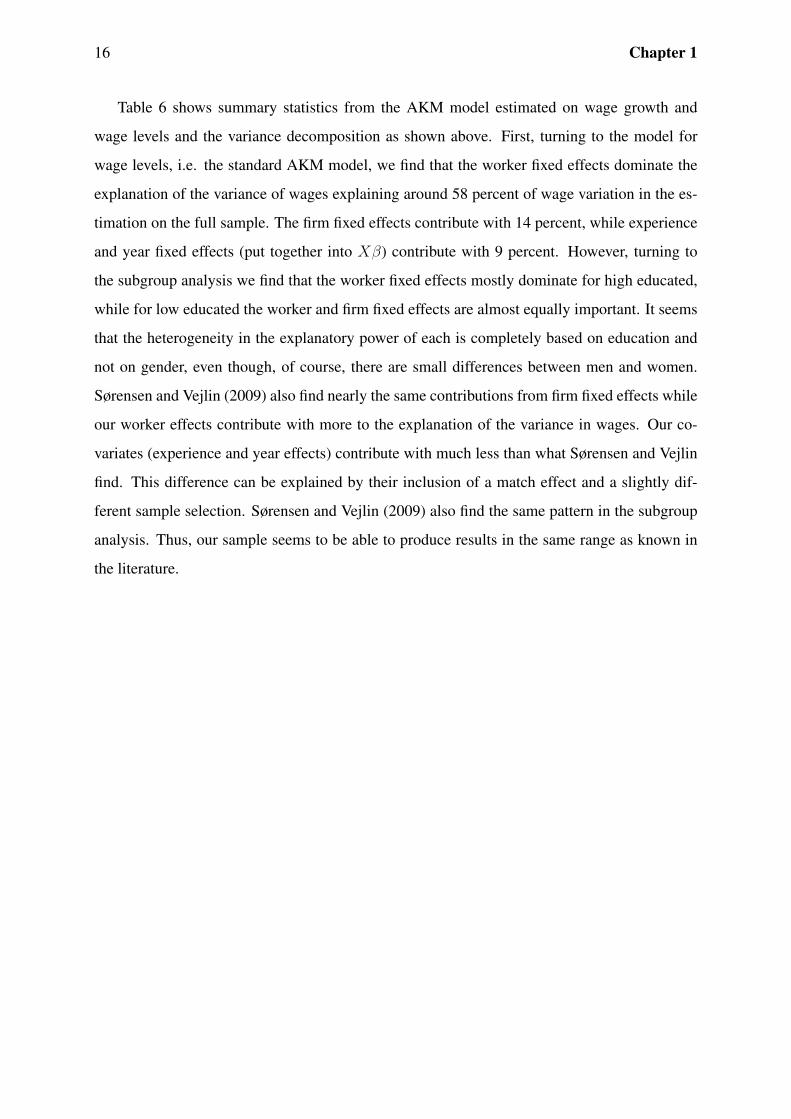
Table 6 shows summary statistics from the AKM model estimated on wage growth and
wage levels and the variance decomposition as shown above. First, turning to the model for
wage levels, i.e. the standard AKM model, we find that the worker fixed effects dominate the
explanation of the variance of wages explaining around 58 percent of wage variation in the es-
timation on the full sample. The firm fixed effects contribute with 14 percent, while experience
and year fixed effects (put together into Xβ) contribute with 9 percent. However, turning to
the subgroup analysis we find that the worker fixed effects mostly dominate for high educated,
while for low educated the worker and firm fixed effects are almost equally important. It seems
that the heterogeneity in the explanatory power of each is completely based on education and
not on gender, even though, of course, there are small differences between men and women.
Sørensen and Vejlin (2009) also find nearly the same contributions from firm fixed effects while
our worker effects contribute with more to the explanation of the variance in wages. Our co-
variates (experience and year effects) contribute with much less than what Sørensen and Vejlin
find. This difference can be explained by their inclusion of a match effect and a slightly dif-
ferent sample selection. Sørensen and Vejlin (2009) also find the same pattern in the subgroup
analysis. Thus, our sample seems to be able to produce results in the same range as known in
the literature.

Worker and Firm Heterogeneity in Wage Growth 17
Table 6: Regression results.
Wage growth Wage levels
Cov(w,Z) Cov(w,Z)
Z Mean Std. Dev. Cov(w,Z) / Var(w) Mean Std. Dev. Cov(w,Z) / Var(w)
Full sample (20,703,609 observations)
w 0.0196 0.1486 0.0221 1.0000 5.2372 0.3072 0.0944 1.0000
θ -0.0780 0.0578 0.0019 0.0868 4.8103 0.2319 0.0543 0.5752
ψ 0.1110 0.0470 0.0009 0.0415 0.2547 0.1107 0.0132 0.1399
Xβ -0.0134 0.0248 0.0005 0.0218 0.1723 0.0940 0.0088 0.0927
ε 0.0000 0.1370 0.0188 0.8499 0.0000 0.1347 0.0181 0.1922
High educated
Men (1,682,834 observations)
w 0.0279 0.1537 0.0236 1.0000 5.6571 0.3354 0.1125 1.0000
θ -0.3121 0.0687 0.0017 0.0739 5.5965 0.2945 0.0645 0.5732
ψ 0.3370 0.0673 0.0018 0.0753 0.1186 0.1392 0.0119 0.1059
Xβ 0.0031 0.0259 0.0005 0.0216 -0.0581 0.1838 0.0141 0.1255
ε 0.0000 0.1400 0.0196 0.8292 0.0000 0.1483 0.0220 0.1954
Women (450,948 observations)
w 0.0297 0.1482 0.0220 1.0000 5.4231 0.3104 0.0963 1.0000
θ 0.0960 0.1130 0.0026 0.1161 5.5190 0.2689 0.0598 0.6208
ψ -0.0581 0.1106 0.0021 0.0961 -0.0851 0.1451 0.0124 0.1289
Xβ -0.0083 0.0217 0.0005 0.0208 -0.0108 0.1315 0.0099 0.1031
ε 0.0000 0.1298 0.0169 0.7670 0.0000 0.1191 0.0142 0.1472
Medium educated
Men (8,823,828 observations)
w 0.0181 0.1488 0.0222 1.0000 5.2778 0.2633 0.0693 1.0000
θ -0.0533 0.0582 0.0016 0.0712 4.8230 0.1817 0.0313 0.4513
ψ 0.0931 0.0546 0.0012 0.0558 0.2670 0.1199 0.0134 0.1935
Xβ -0.0218 0.0238 0.0005 0.0220 0.1878 0.0882 0.0071 0.1025
ε 0.0000 0.1373 0.0189 0.8509 0.0000 0.1324 0.0175 0.2527
Women (3,443,791 observations)
w 0.0259 0.1406 0.0198 1.0000 5.0995 0.2546 0.0648 1.0000
θ -0.2304 0.0720 0.0020 0.1024 4.5700 0.1774 0.0277 0.4271
ψ 0.2595 0.0650 0.0013 0.0661 0.3321 0.1104 0.0103 0.1591
Xβ -0.0032 0.0276 0.0006 0.0280 0.1974 0.1181 0.0127 0.1955
ε 0.0000 0.1260 0.0159 0.8036 0.0000 0.1190 0.0141 0.2183
Low educated
Men (3,996,477 observations)
w 0.0151 0.1554 0.0241 1.0000 5.1837 0.2447 0.0599 1.0000
θ 0.0051 0.0720 0.0020 0.0841 4.6726 0.1620 0.0211 0.3531
ψ 0.0359 0.0704 0.0019 0.0781 0.3344 0.1432 0.0175 0.2915
Xβ -0.0258 0.0275 0.0006 0.0267 0.1767 0.0783 0.0058 0.0976
ε 0.0000 0.1400 0.0196 0.8111 0.0000 0.1242 0.0154 0.2577
This table continues on the next page.
Note: Z in columns 4, 5, 9 and 10 denotes w, θ, ψ, Xβ or ε depending on the row in question.

18 Chapter 1
Table 6 – continued from previous page.
Wage growth Wage levels
Cov(w,Z) Cov(w,Z)
Z Mean Std. Dev. Cov(w,Z) / Var(w) Mean Std. Dev. Cov(w,Z) / Var(w)
Women (1,914,928 observations)
w 0.0160 0.1376 0.0189 1.0000 5.0194 0.2277 0.0518 1.0000
θ 0.0526 0.0785 0.0020 0.1063 4.7302 0.1593 0.0178 0.3429
ψ -0.0577 0.0738 0.0016 0.0825 0.1063 0.1420 0.0154 0.2972
Xβ 0.0212 0.0279 0.0005 0.0277 0.1830 0.0853 0.0064 0.1244
ε 0.0000 0.1218 0.0148 0.7836 0.0000 0.1105 0.0122 0.2355
Note: Z in columns 4, 5, 9 and 10 denotes w, θ, ψ, Xβ or ε depending on the row in question.
Our results of the variance decomposition yield much lower estimates of the degree of ex-
planation of the variance in wage levels than those given by most former literature. One ex-
planation of this can be that we use much longer panels than e.g. Abowd et al. (1999) (panel
covering 1976-1987, excluding 1981 and 1983), Abowd et al. (2002) (same panel length as
AKM) and Barth and Dale-Olsen (2003) (panel covering 1989-1997). Figures 2 to 4 show the
variance decomposition (equation (6)) plotted for each subgroup against the number of times
we have observed the individual worker. The development in contribution to the variance of
wages is almost the same for all three subgroups where the worker effects seem to be mostly
negatively affected by the length of the panels while the contributions from firm effects are rel-
atively constant and the covariates experience increasing contribution to the variance of wages
for all subgroups. AKM, Abowd et. al, and Barth and Dale-Olsen all use unbalanced panels
as we do, and they could thus possibly have an upward biased worker effect. It is a subject
for further research whether the estimated worker and firm effects are dependent on the panel
lengths at hand.
Now turning to the main analysis of the wage growth equation. For the full sample the
variation in the worker effect explains 8.7 percent, the firm effect explains 4.2 percent, and
experience and year effects explain 2.2 percent. I.e., as in the regressions on wage levels,
the most important component is the worker fixed effect. When we estimate the model on
the six subgroups of gender and educational level an interesting pattern emerges. It seems
that especially the worker effect, but to some extent also the firm effect, is more important in
explaining women’s wage growth. In all subgroups with an equal amount of education the
explanatory power of both the worker and the firm effect is higher for women than for men.

Worker and Firm Heterogeneity in Wage Growth 19
Figure 2: Degree of explanation given by worker effects, firm effects and covariates according to the variancedecomposition plotted against number of person-years observed.
0.2
.4.6
.81
Degre
e o
f expla
nation
1 5 9 13 17 21 25Number of years observed
Worker effects Firm effects
Covariates Residuals
High educated men
0.2
.4.6
.81
Degre
e o
f expla
nation
1 5 9 13 17 21 25Number of years observed
Worker effects Firm effects
Covariates Residuals
High educated women
Figure 3: Degree of explanation given by worker effects, firm effects and covariates according to the variancedecomposition plotted against number of person-years observed.
0.2
.4.6
.81
Degre
e o
f expla
nation
1 5 9 13 17 21 25Number of years observed
Worker effects Firm effects
Covariates Residuals
Medium educated men
0.2
.4.6
.81
Degre
e o
f expla
nation
1 5 9 13 17 21 25Number of years observed
Worker effects Firm effects
Covariates Residuals
Medium educated women

20 Chapter 1
Figure 4: Degree of explanation given by worker effects, firm effects and covariates according to the variancedecomposition plotted against number of person-years observed.
0.2
.4.6
.81
Degre
e o
f expla
nation
1 5 9 13 17 21 25Number of years observed
Worker effects Firm effects
Covariates Residuals
Low educated men
0.2
.4.6
.81
Degre
e o
f expla
nation
1 5 9 13 17 21 25Number of years observed
Worker effects Firm effects
Covariates Residuals
Low educated women
The clear pattern from the wage level estimation, where worker effects were most important for
high educated, is nearly not present in wage growth. In general, worker effects explain around 8
to 12 percent, firm effects explain around 4 to 10 percent, and experience and the year dummies
together explain 2 to 3 percent. That is, the most important component of wage growth is worker
specific differences, but it also seems that firm heterogeneity plays a relatively important role
in determining wage growth compared to determining variance in wage levels. We also see that
experience and year dummies explain a very small fraction of the variation in wage growth.
This is not a surprising result though, since (in the Robustness section below (table A1 column
(1))) we find R2 = 0.024 when running a simple OLS regression without including any fixed
effects.
Compared to the model for wage levels the degree of explanation is dramatically smaller
for wage growth. I.e. we cannot explain the variation in wage growth as precisely as we can
explain the variation in the level of wages. Also for wage levels the most important component
is the worker fixed effect, while the firm fixed effect and experience and year dummies seem
to explain an almost equal share. The latter part is in contrast to the model for wage growth
where the covariates constantly contribute with around half the share of the contribution given
by firm fixed effects. A possible explanation of this can simply be that there is a relatively higher
variance in the error term when analyzing wage growth than wage levels. Given the relatively

Worker and Firm Heterogeneity in Wage Growth 21
low contribution by firm effects compared to the worker effects and the residual, one could
doubt the significance of the firm effects. We have tested this for each subgroup using a simple
F-test with the hypothesis that the model with firm effects included does not provide a significant
better fit of wage growth (and levels) than a model without firm fixed effects included. The test
gives a p-value of zero for all subgroups for both wage growth and wage levels.11
Table 7 shows the correlation structure of the two models for wage growth and wage levels.
In levels we see that there is a small but positive correlation between the firm effect and the
worker effect in the full sample, but when we turn to the subsamples we find a negative cor-
relation. This is also found by Sørensen and Vejlin (2009). In the wage growth equation we
find a strong negative correlation between the firm effect and the worker effect. I.e. workers
with high wage growth are on average in firms with low wage growth. One reason could be the
negative bias between worker and firm effects, see e.g. Bagger and Lentz (2008). Furthermore,
Andrews et al. (2008) show that the magnitude of this bias is increasing in the size of the error
term variance which explains our much stronger correlation than earlier studies such as e. g.
Abowd et al. (2002) and Gruetter and Lalive (2004). The negative correlation between worker
and firm effects is consistently stronger for women than for men throughout the educational
subgroups, and does not differ much for men whether they are high, medium or low educated,
whereas the correlation is much higher (in absolute terms) for high educated women than for
low and medium educated women. The difference in the magnitude of the correlation between
worker and firm effects when analyzing wage growth and wage levels can to a large extent be
explained by a much lower standard deviation of worker and firm effects in the wage growth
estimations compared to wage levels.
11The test with the lowest F-statistic is high educated women, wage growth at F = 52, 393. The correspondingcritical value on a significance level of five percent is F (92, 036 − 20, 277; 450, 948 − 20, 277) = 1.009 and thefirm effects are thus highly significant.

22 Chapter 1
Table 7: Correlation structure, full AKM model, wage growth and wage levels.
Wage growth Wage levels
w θ ψ Xβ ε w θ ψ Xβ ε
Full sample
w 1.0000 0.2232 0.1313 0.1306 0.9219 1.0000 0.7619 0.3883 0.3029 0.4384
θ 0.2232 1.0000 -0.4749 -0.0931 0.0000 0.7619 1.0000 0.0302 -0.0124 0.0000
ψ 0.1313 -0.4749 1.0000 -0.0008 0.0000 0.3883 0.0302 1.0000 0.0169 0.0000
Xβ 0.1306 -0.0931 -0.0008 1.0000 0.0000 0.3029 -0.0124 0.0169 1.0000 0.0000
ε 0.9219 0.0000 0.0000 0.0000 1.0000 0.4384 0.0000 0.0000 0.0000 1.0000
High educated
Men
w 1.0000 0.1652 0.1720 0.1285 0.9106 1.0000 0.6528 0.2551 0.2290 0.4420
θ 0.1652 1.0000 -0.6020 -0.1089 0.0000 0.6528 1.0000 -0.1225 -0.3182 0.0000
ψ 0.1720 -0.6020 1.0000 0.0198 0.0000 0.2551 -0.1225 1.0000 -0.0955 0.0000
Xβ 0.1285 -0.1089 0.0198 1.0000 0.0000 0.2290 -0.3182 -0.0955 1.0000 0.0000
ε 0.9106 0.0000 0.0000 0.0000 1.0000 0.4420 0.0000 0.0000 0.0000 1.0000
Women
w 1.0000 0.1523 0.1288 0.1422 0.8758 1.0000 0.7165 0.2756 0.2434 0.3837
θ 0.1523 1.0000 -0.8131 -0.0229 0.0000 0.7165 1.0000 -0.1768 -0.1589 0.0000
ψ 0.1288 -0.8131 1.0000 0.0178 0.0000 0.2756 -0.1768 1.0000 -0.0911 0.0000
Xβ 0.1422 -0.0229 0.0178 1.0000 0.0000 0.2434 -0.1589 -0.0911 1.0000 0.0000
ε 0.8758 0.0000 0.0000 0.0000 1.0000 0.3837 0.0000 0.0000 0.0000 1.0000
Medium educated
Men
w 1.0000 0.1821 0.1523 0.1379 0.9225 1.0000 0.6540 0.4249 0.3061 0.5027
θ 0.1821 1.0000 -0.5467 -0.0523 0.0000 0.6540 1.0000 -0.0463 -0.0449 0.0000
ψ 0.1523 -0.5467 1.0000 -0.0039 0.0000 0.4249 -0.0463 1.0000 0.0048 0.0000
Xβ 0.1379 -0.0523 -0.0039 1.0000 0.0000 0.3061 -0.0449 0.0048 1.0000 0.0000
ε 0.9225 0.0000 0.0000 0.0000 1.0000 0.5027 0.0000 0.0000 0.0000 1.0000
Women
w 1.0000 0.1999 0.1429 0.1428 0.8964 1.0000 0.6130 0.3668 0.4215 0.4672
θ 0.1999 1.0000 -0.6275 -0.1128 0.0000 0.6130 1.0000 -0.1121 -0.0759 0.0000
ψ 0.1429 -0.6275 1.0000 0.0098 0.0000 0.3668 -0.1121 1.0000 0.0243 0.0000
Xβ 0.1428 -0.1128 0.0098 1.0000 0.0000 0.4215 -0.0759 0.0243 1.0000 0.0000
ε 0.8964 0.0000 0.0000 0.0000 1.0000 0.4672 0.0000 0.0000 0.0000 1.0000
Low educated
Men
w 1.0000 0.1816 0.1723 0.1512 0.9006 1.0000 0.5333 0.4983 0.3048 0.5077
θ 0.1816 1.0000 -0.6030 -0.0478 0.0000 0.5333 1.0000 -0.1693 -0.0927 0.0000
ψ 0.1723 -0.6030 1.0000 -0.0077 0.0000 0.4983 -0.1693 1.0000 0.0786 0.0000
Xβ 0.1512 -0.0478 -0.0077 1.0000 0.0000 0.3048 -0.0927 0.0786 1.0000 0.0000
ε 0.9006 0.0000 0.0000 0.0000 1.0000 0.5077 0.0000 0.0000 0.0000 1.0000
This table continues on the next page.

Worker and Firm Heterogeneity in Wage Growth 23
Table 7 – continued from previous page.
Wage growth Wage levels
w θ ψ Xβ ε w θ ψ Xβ ε
Women
w 1.0000 0.1862 0.1537 0.1366 0.8852 1.0000 0.4901 0.4764 0.3319 0.4853
θ 0.1862 1.0000 -0.6717 -0.1175 0.0000 0.4901 1.0000 -0.2549 -0.1348 0.0000
ψ 0.1537 -0.6717 1.0000 0.0015 0.0000 0.4764 -0.2549 1.0000 0.0826 0.0000
Xβ 0.1366 -0.1175 0.0015 1.0000 0.0000 0.3319 -0.1348 0.0826 1.0000 0.0000
ε 0.8852 0.0000 0.0000 0.0000 1.0000 0.4853 0.0000 0.0000 0.0000 1.0000
4.2 Within- and Between-Firm Wage Growth
So far, all results have been solely focusing on wage growth. Here we distinguish between
within- and between-firm wage growth. We have divided our samples of the full sample, men
and women, into those who have made a transition into a new job and those who have not.
Table 8 shows the results of within- and between-firm wage growth. First, we have included
transition as a dummy in the covariates of the basis regression to see whether transition itself
can help explain wage growth variation. The first five rows of Table 8 contain results from this
exercise. Comparison with Table 6 reveals that inclusion of this transition dummy contributes
no extra explanatory power to the model. Second, we regress the standard model for men
and women together as well as for men and women separately for both the sample of workers
staying at the same employer (within-firm wage growth) and workers making a transition into a
new job (between-firm wage growth). Two very interesting results leap out of Table 8; first, the
overall explanatory power of the model rises for both samples. We are able to explain 20 percent
of the variance in within-firm wage growth and as much as 46 percent of the full sample and
male between-firm wage growth variation and even 58 percent of female between-firm wage
growth variation. Second, the relative firm specific importance in wage growth variation rises
dramatically when analyzing between-firm wage growth.
Table 9 shows the correlation structure of the within- and between-firm wage growth analy-
sis. Comparing with the baseline model, we see that the correlation structure of worker and firm
specific effects changes only very little and it retains its overall structure with worker specific
effects being highly negatively correlated with firm specific effects, although the correlation is
slight lesser in the between-firm wage growth sample than it is in the within-firm sample.

24 Chapter 1
Tabl
e8:
Rob
ustn
ess
chec
ksfo
rwag
egr
owth
;Reg
ress
ion
Res
ults
.
All
Men
Wom
enCov(w,Z
)/Cov(w,Z
)/Cov(w,Z
)/Z
Mea
nSt
d.D
evCov(w,Z
)Var(w
)M
ean
Std.
Dev
Cov(w,Z
)Var(w
)M
ean
Std.
Dev
Cov(w,Z
)Var(w
)
Full
Sam
ple
(20,
703,
609
obs)
Full
Sam
ple
(14,
619,
789
obs)
Full
Sam
ple
(5,9
49,1
55ob
s)w
0.01
960.
1486
0.02
211.
0000
0.01
840.
1514
0.02
291.
0000
0.02
290.
1407
0.01
981.
0000
θ-0
.075
00.
0576
0.00
190.
0866
-0.0
755
0.05
810.
0018
0.07
77-0
.224
80.
0687
0.00
210.
1082
ψ0.
1094
0.04
700.
0009
0.04
150.
1104
0.05
070.
0011
0.04
810.
2537
0.05
940.
0011
0.05
55Xβ∗
-0.0
148
0.02
480.
0005
0.02
21-0
.016
50.
0249
0.00
050.
0213
-0.0
060
0.02
600.
0005
0.02
59ε
0.00
000.
1370
0.01
880.
8499
0.00
000.
1399
0.01
960.
8530
0.00
000.
1267
0.01
600.
8104
Tran
sitio
n=
0(1
7,22
7,14
4ob
s)Tr
ansi
tion
=0
(12,
074,
930
obs)
Tran
sitio
n=
0(4
,976
,707
obs)
w0.
0194
0.13
270.
0176
1.00
000.
0178
0.13
370.
0179
1.00
000.
0235
0.12
890.
0166
1.00
00θ
0.04
130.
0599
0.00
250.
1392
0.06
880.
0592
0.00
230.
1286
-0.0
741
0.07
060.
0027
0.16
14ψ
-0.0
077
0.03
960.
0005
0.02
94-0
.039
80.
0412
0.00
060.
0335
0.11
230.
0540
0.00
070.
0405
Xβ?
-0.0
141
0.02
350.
0005
0.02
64-0
.011
20.
0237
0.00
040.
0250
-0.0
148
0.02
410.
0005
0.03
12ε
0.00
000.
1191
0.01
420.
8050
0.00
000.
1206
0.01
450.
8129
0.00
000.
1129
0.01
270.
7669
Tran
sitio
n=
1(3
,374
,561
obs)
Tran
sitio
n=
1(2
,469
,392
obs)
Tran
sitio
n=
1(8
82,6
27ob
s)w
0.02
080.
2104
0.04
431.
0000
0.02
110.
2168
0.04
701.
0000
0.02
010.
1908
0.03
641.
0000
θ0.
0046
0.13
670.
0128
0.28
890.
0304
0.13
760.
0125
0.26
52-0
.915
50.
1510
0.01
280.
3512
ψ0.
0731
0.11
400.
0070
0.15
900.
0578
0.12
210.
0084
0.17
840.
9575
0.13
340.
0077
0.21
26Xβ?
-0.0
569
0.03
370.
0009
0.02
07-0
.067
10.
0340
0.00
100.
0207
-0.0
219
0.03
460.
0008
0.02
26ε
0.00
000.
1534
0.02
350.
5314
0.00
000.
1587
0.02
520.
5356
0.00
000.
1227
0.01
510.
4135
∗ Ful
lsam
ple;
Cov
aria
tes
incl
ude:
expe
rien
ce,e
xper
ienc
esq
uare
d,ye
aref
fect
san
da
tran
sitio
ndu
mm
y.?
Tran
sitio
nsa
mpl
es;C
ovar
iate
sin
clud
e:ex
peri
ence
,exp
erie
nce
squa
red
and
year
effe
cts.

Worker and Firm Heterogeneity in Wage Growth 25
Tabl
e9:
Rob
ustn
ess
chec
ksfo
rwag
egr
owth
;Cor
rela
tion
Stru
ctur
e.
All
Men
Wom
enZ
wθ
ψXβ
εw
θψ
Xβ
εw
θψ
Xβ
ε
Full
Sam
ple
(20,
703,
609
obs)
Full
Sam
ple
(14,
619,
789
obs)
Full
Sam
ple
(5,9
49,1
55ob
s)w
1.00
000.
2025
0.14
350.
1296
0.92
361.
0000
0.20
250.
1435
0.12
960.
9236
1.00
000.
2216
0.13
150.
1401
0.90
02θ
0.20
251.
0000
-0.4
978
-0.0
876
0.00
000.
2025
1.00
00-0
.497
8-0
.087
60.
0000
0.22
161.
0000
-0.5
935
-0.0
883
0.00
00ψ
0.14
35-0
.497
81.
0000
-0.0
034
0.00
000.
1435
-0.4
978
1.00
00-0
.003
40.
0000
0.13
15-0
.593
51.
0000
-0.0
038
0.00
00Xβ∗
0.12
96-0
.087
6-0
.003
41.
0000
0.00
000.
1296
-0.0
876
-0.0
034
1.00
000.
0000
0.14
01-0
.088
3-0
.003
81.
0000
0.00
00ε
0.92
360.
0000
0.00
000.
0000
1.00
000.
9236
0.00
000.
0000
0.00
001.
0000
0.90
020.
0000
0.00
000.
0000
1.00
00
Tran
sitio
n=
0(1
7,22
7,14
4ob
s)Tr
ansi
tion
=0
(12,
074,
930
obs)
Tran
sitio
n=
0(4
,976
,707
obs)
w1.
0000
0.29
050.
1089
0.14
060.
9016
1.00
000.
2905
0.10
890.
1406
0.90
161.
0000
0.29
460.
0968
0.16
700.
8757
θ0.
2905
1.00
00-0
.447
8-0
.081
10.
0000
0.29
051.
0000
-0.4
478
-0.0
811
0.00
000.
2946
1.00
00-0
.588
3-0
.036
30.
0000
ψ0.
1089
-0.4
478
1.00
00-0
.003
30.
0000
0.10
89-0
.447
81.
0000
-0.0
033
0.00
000.
0968
-0.5
883
1.00
000.
0006
0.00
00Xβ?
0.14
06-0
.081
1-0
.003
31.
0000
0.00
000.
1406
-0.0
811
-0.0
033
1.00
000.
0000
0.16
70-0
.036
30.
0006
1.00
000.
0000
ε0.
9016
0.00
000.
0000
0.00
001.
0000
0.90
160.
0000
0.00
000.
0000
1.00
000.
8757
0.00
000.
0000
0.00
001.
0000
Tran
sitio
n=
1(3
,374
,561
obs)
Tran
sitio
n=
1(2
,469
,392
obs)
Tran
sitio
n=
1(8
82,6
27ob
s)w
1.00
000.
4178
0.31
690.
1323
0.73
191.
0000
0.41
780.
3169
0.13
230.
7319
1.00
000.
4440
0.30
430.
1246
0.64
31θ
0.41
781.
0000
-0.3
813
-0.0
147
0.00
000.
4178
1.00
00-0
.381
3-0
.014
70.
0000
0.44
401.
0000
-0.4
884
-0.0
313
0.00
00ψ
0.31
69-0
.381
31.
0000
-0.0
268
0.00
000.
3169
-0.3
813
1.00
00-0
.026
80.
0000
0.30
43-0
.488
41.
0000
-0.0
459
0.00
00Xβ?
0.13
23-0
.014
7-0
.026
81.
0000
0.00
000.
1323
-0.0
147
-0.0
268
1.00
000.
0000
0.12
46-0
.031
3-0
.045
91.
0000
0.00
00ε
0.73
190.
0000
0.00
000.
0000
1.00
000.
7319
0.00
000.
0000
0.00
001.
0000
0.64
310.
0000
0.00
000.
0000
1.00
00∗ F
ulls
ampl
e;C
ovar
iate
sin
clud
e:ex
peri
ence
,exp
erie
nce
squa
red,
year
effe
cts
and
atr
ansi
tion
dum
my.
?Tr
ansi
tion
sam
ples
;Cov
aria
tes
incl
ude:
expe
rien
ce,e
xper
ienc
esq
uare
dan
dye
aref
fect
s.

26 Chapter 1
5 Robustness
To analyze the robustness of our results we have run several different specifications of the
model. First, to check if the low contribution in the wage growth variance decomposition by
covariates results from too few variables added, we have included information on marital status,
children, the size of the firm this period and one period before to the covariates. Second, we
regress seven different variations of the model to see if the results change between them. Table
A1 (in the appendix) shows these robustness checks. Column (3) is the baseline model where
the only difference compared to the full sample part of Table 6 (row 2 - 6) is that a very small
fraction of the worker effect and the residuals has been absorbed by the covariates with the
inclusion of the extra variables. The difference between column (3) and the full sample part
of Table 6 is not significant on any conventional levels, though, and we have thus no reason
to think that excluding the extra covariates alters our results.12 Column (1) is the original OLS
regression and the covariates themselves are seen to explain 2.24 percent of the variance in wage
growth; The same contribution up to four decimals as in the baseline model with both worker
and firm fixed effects added. We thus seem to be able to extract truly unobserved heterogeneity
by including the fixed effects. The importance of the covariates does not alter much if we
include either firm effects (column (2)) or worker effects (column (6)) to the model only, and
lies between 2.1 and 2.9 percent. The contribution from the unobserved worker heterogeneity
on the variance of wage growth is relatively robust over columns (3) to (6) but the importance
of the unobserved firm heterogeneity seems to increase for models with worker fixed effects
included (columns (3) and (5)) than without worker specific effects (columns (2) and (7)). In
the end, our model specification seems to be relatively robust.13
Table A2 and A3 list the same robustness checks as Table A1 but for growth in wages
over two and three periods, respectively. Comparing the baseline model (column (3)) in Table
A2 and A3 with Table 6 shows that the interrelationship between the worker fixed effects,
the firm fixed effects and the covariates remains relatively constant with the firm effects being
twice as important as the covariates and the worker effects again twice as important as the firm
effects. When analyzing higher period wage growth one would expect the different components
to absorb some of the residual explanation compared to one-period wage growth; the covariates12F-test not shown, but available upon request.13One could argue a more important experience measure were firm or industry tenure instead of overall experi-
ence. We have tried several different specifications, letting firm or industry tenure be an extra covariate or replaceexperience and experience squared with tenure and tenure squared. None of these operations led to any significantchanges in regression results or the correlation structure.

Worker and Firm Heterogeneity in Wage Growth 27
because experience increases. the firm effect because firms paying consistently higher than
average period-to-period wage growth will be paying even higher two-period wage growth.
Finally, the worker effect will follow a similar pattern and be more important for describing
the variance in wage growth over two periods than in only one period. Likewise, these effects
would be expected to be even more clear when analyzing wage growth over three periods. Table
A2 and A3 indeed show that the contribution to the variance in wage growth rises when moving
from one-period to two- and three-period wage growth as we would expect. However, it is
important to note that the relative contribution does not change much. Furthermore, Table A2
and A3 support our conjecture that the part of the lack in wage growth variance explanatory
power compared to analysis of wage level variation can be contributed to a higher variance in
the error term as we are able to extract more and more explanatory power from the error term
when using longer period wage growth.
As a final robustness check, one could argue that using size of the firm as the only firm
specific control would not capture wage policies within firms. We have thus regressed the
baseline model with average firm wage growth within each year as covariate together with
worker experience and experience squared to see if this changes the results dramatically. Table
A4 shows the regression results and following correlation structure.
Comparing the results with those of the baseline model (table 6) reveals that including aver-
age firm wage growth in the regression lowers the contribution to the variance of wage growth
by firm effects to 2.6 percent while covariates become much more important. Including average
firm wage growth thus raise the explanatory power of observables from 2.2 percent to 9.6 per-
cent. There is no significant change in the contribution of worker specific effects to the variance
of wage growth. However, it is not surprising that including average firm wage growth in the
regression lowers the importance of firm effects and rises the effect of the covariates. A positive
firm effect firm is characterized by being one that pays higher than average wage growth given
the observables so including exactly the characterization into the observables will automatically
bias the results towards the covariates. The correlation structure does not change much by this
inclusion, and especially the correlation between worker and firm effects remains the same as
for the baseline model.

28 Chapter 1
6 Conclusions
This paper estimates a regression model for individual wage growth incorporating fixed worker
and firm effects. We find that these worker and firm fixed effects influence wage growth very
differently from the way they influence wages in levels. We have decomposed the variance of
wage growth and wage levels into contributions from fixed worker effects, fixed firm effects,
observable experience and year effects and what is left unexplained. We found that while worker
effects could contribute with around 60 percent for high educated workers, around 42 percent
for medium educated workers and around 35 percent for low educated workers of the variance
in wage levels we are only able to attribute around 7 to 12 percent to worker effects for all three
educational groups of the variance in wage growth to fixed worker effects. The same pattern
seems to be the case for firm effects, for which we can attribute from 10 to 30 percent of the
contribution to the variance in wage levels, while they are estimated to explain 4 to 10 percent
of the variance in wage growth. Finally, the amount of variance left unexplained is much higher
for wage growth than it is for wage levels ranging from 76 percent to 85 percent for subgroups
and 85 percent for the full sample in wage growth versus 14 to 25 percent for subgroups and 19
percent for the full sample in wage levels.
However, the amount of variance that we can explain increases from 15 percent to 30 per-
cent, when we use three-period wage growth instead of one-period growth. Importantly, the
interrelationship between the components does not alter considerably when moving from using
one-period wage growth to either two- or three-period wage growth, as the worker effect keeps
having around twice the explanatory power as firm effects which then have almost twice the
explanatory power as observable covariates.
We also find a very strong negative correlation between fixed worker and fixed firm effects
in wage growth, much stronger than usually found for AKM wage level models. Some of
this difference can be attributed to our estimated worker and firm effects having much lower
standard deviation than worker and firm effects in wage levels. However, the major explanation
lies in the high residual variance which Andrews et al. (2008) have shown to be important for
the size of the correlation in worker and firm effects.

Worker and Firm Heterogeneity in Wage Growth 29
ReferencesAbowd, J., H. Finer and F. Kramarz (1999), Individual and Firm Heterogeneity in Compen-
sation: An Analysis of Matched Longitudinal Employer and Employee Data for the State ofWashington, in J. Haltiwanger, J. Lane, J. Spletzer and K. Troske (eds.), The Creation andAnalysis of Employer-Employee Matched Data, North-Holland, 3–24.
Abowd, J. M., R. H. Creecy and F. Kramarz (2002), Computing Person and Firm Effects Us-ing Linked Longitudinal Employer-Employee Data, Technical Paper 2002-06, U.S. CensusBureau.
Abowd, J. M. and F. Kramarz (1999), The Analysis of Labor Markets using Matched Employer-Employee Data , vol. 3 of Handbook of Labor Economics, chap. 40, Elsevier Science B.V.,2629–2710.
Abowd, J. M., F. Kramarz and D. N. Margolis (1999), High Wage Workers and High WageFirms, Econometrica, 67(2): 251–333.
Andrews, M. J., L. Gill, T. Schank and R. Upward (2008), High wage workers and low wagefirms: negative assortative matching or limited mobility bias?, Journal of the Royal StatisticalSociety, A(2008) 171(Part 3): 673–697.
Bagger, J., F. Fontaine, F. Postel-Vinay and J.-M. Robin (2007), A Tractable Equilibrium SearchModel with Experience Accumulation, Working Paper.
Bagger, J. and R. Lentz (2008), An Empirical Model of Wage Dispersion with Sorting, WorkingPaper.
Baker, M. (1997), Growth-Rate Heterogeneity and the Covariance Structure of Life-Cycle Earn-ings, Journal of Labor Economics, 15(2): 338–375.
Barth, E. and H. Dale-Olsen (2003), Assortative matching in the labor market? Stylized factsabout workers and plants, Institute for Social Research, Oslo, Norway.
Connolly, H. and P. Gottschalk (2006), Differences in Wage Growth by Education Level: DoLess-Educated Workers Gain Less from Work Experience?, IZA Discussion Papers 2331, In-stitute for the Study of Labor (IZA).
Eeckhout, J. and P. Kircher (2009), Identifying Sorting - In Theory, Working Paper.
Gladden, T. and C. Taber (2009), The Relationship Between Wage Growth and Wage Levels,Journal of Applied Econometrics, 24: 914–932.
Gruetter, M. and R. Lalive (2004), The Importance of Firms in Wage Determination, IEW -Working Papers 207, Institute for Empirical Research in Economics - IEW.
Heckman, J. J., L. J. Lochner and P. E. Todd (2003), Fifty Years of Mincer Earnings Regres-sions, NBER Working Papers 9732, National Bureau of Economic Research, Inc.
Kramarz, F., S. Machin and A. Ouazad (2009), What Makes a Test Score? The RespectiveContributions of Pupils, Schools and Peers in Achievement in English Primary Education,CEE Discussion Papers CEEDP0102, CEE.
Lopes de Melo, R. (2008), Sorting In the Labor Market: Theory and Measurement, WorkingPaper, Yale.
Mincer, J. (1958), Investment in Human Capital and Personal Income Distribution, The Journalof Political Economy, 66(4): 281–302.
Mincer, J. A. (1974), Schooling, Experience, and Earnings, New York: Columbia UniversityPress.

30 Chapter 1
Mortensen, D. T. (2005), Wage Dispersion - Why are similar workers paid differently, First MITPress paperback edition.
Postel-Vinay, F. and J.-M. Robin (2002), Equilibrium Wage Dispersion with Worker and Em-ployer Heterogeneity, Econometrica, 70(6): 2295–2350.
Shimer, R. (2005), The Assignment of Workers in an Economy with Coordination Frictions,Journal of Political Economy, 113(5): 996–1025.
Sørensen, K. L. and R. M. Vejlin (2011), Return to Experience and Initial Wage Level: Do LowWage Workers Catch Up?, Working Paper; School of Economics and Management, AarhusUniversity.
Sørensen, T. and R. Vejlin (2009), The Importance of Worker, Firm and Match Fixed Effectsin the Formation of Wages, Working Paper; School of Economics and Management, AarhusUniversity.
Woodcock, S. (2008), Match Effects, Discussion Papers. Department of Economics, SimonFraser University.

Worker and Firm Heterogeneity in Wage Growth 31
AppendicesA Tables
Table A1: Results from the wage growth variance decomposition for different models.
Degree of contribution to the variance of wage growth
(1) (2) (3) (4) (5) (6) (7)
θ - - 0.0864 0.0890 0.0872 0.0905 -ψ - 0.0352 0.0415 - 0.0436 - 0.0377Xβ 0.0224 0.0292 0.0224 - - 0.0212 -ε 0.9776 0.9356 0.8497 0.9110 0.8692 0.8883 0.9623
Components included
θ no no yes yes yes yes noψ no yes yes no yes no yesXβ yes yes yes no no yes noObservations 20,703,609 20,703,609 20,703,609 20,703,609 20,703,609 20,703,609 20,703,609Workers 2,083,391 2,083,391 2,083,391 2,083,391 2,083,391 2,083,391 2,083,391Firms 295,034 295,034 295,034 295,034 295,034 295,034 295,034Covariates 7 7 7 0 0 7 0
Note: Covariates included are; Experience, experience squared, married, children, firm size, lagged firm sizeand year dummies.
Table A2: Results from the two-period wage growth variance decomposition for different models.
Degree of contribution to the variance of two-period wage growth
(1) (2) (3) (4) (5) (6) (7)
θ - - 0.1231 0.1245 0.1221 0.1327 -ψ - 0.0554 0.0645 - 0.0706 - 0.0601Xβ 0.0269 0.0416 0.0317 - - 0.0297 -ε 0.9731 0.9030 0.7807 0.8755 0.8073 0.8376 0.9399
Components included
θ no no yes yes yes yes noψ no yes yes no yes no yesXβ yes yes yes no no yes noObservations 19,583,137 19,583,137 19,583,137 19,583,137 19,583,137 19,583,137 19,583,137Workers 1,865,333 1,865,333 1,865,333 1,865,333 1,865,333 1,865,333 1,865,333Firms 276,391 276,391 276,391 276,391 276,391 276,391 276,391Covariates 3 3 3 0 0 3 0
Note: Covariates included are; Experience, experience squared and year dummies.

32 Chapter 1
Table A3: Results from the three-period wage growth variance decomposition for different models.
Degree of contribution to the variance of three-period wage growth
(1) (2) (3) (4) (5) (6) (7)
θ - - 0.1712 0.1742 0.1667 0.1868 -ψ - 0.0698 0.0765 - 0.0879 - 0.0774Xβ 0.0397 0.0528 0.0407 - - 0.0382 -ε 0.9603 0.8774 0.7116 0.8258 0.7454 0.7750 0.9226
Components included
θ no no yes yes yes yes noψ no yes yes no yes no yesXβ yes yes yes no no yes noObservations 17,680,262 17,680,262 17,680,262 17,680,262 17,680,262 17,680,262 17,680,262Workers 1,724,736 1,724,736 1,724,736 1,724,736 1,724,736 1,724,736 1,724,736Firms 254,920 254,920 254,920 254,920 254,920 254,920 254,920Covariates 3 3 3 0 0 3 0
Note: Covariates included are; Experience, experience squared and year dummies.
Table A4: Wage growth regression results with average firm wage growth included in the covariates.
Cov(w,Z)Z Mean Std. Dev. Cov(w,Z) /V ar(w)
Full sample (19,758,785 obs)w 0.0193 0.1465 0.0215 1.0000θ 0.0310 0.0567 0.0019 0.0893ψ -0.0135 0.0422 0.0006 0.0259Xβ 0.0017 0.0474 0.0021 0.0964ε 0.0000 0.1301 0.0169 0.7884
Corr. w θ ψ Xβ ε
w 1.0000 0.2307 0.0898 0.2979 0.8879θ 0.2307 1.0000 -0.4903 -0.0467 0.0000ψ 0.0898 -0.4903 1.0000 -0.0261 0.0000Xβ 0.2979 -0.0467 -0.0261 1.0000 0.0000ε 0.8879 0.0000 0.0000 0.0000 1.0000

Chapter 2
Wage Sorting Trends


Wage Sorting Trends∗
Jesper Bagger† Rune Vejlin‡
Royal Holloway College Aarhus University
Kenneth L. Sørensen§
Aarhus University
Abstract
Using a population-wide Danish Matched Employer-Employee panel from 1980-2006,
we document a strong trend towards more positive assortative wage sorting. The correlation
between worker and firm fixed effects estimated from a log wage regression increases from
−.07 in 1981 to .14 in 2001. The nonstationary wage sorting pattern is not due to com-
positional changes in the labor market, primarily occurs among high wage workers, and
comprises 41 percent of the increase in the standard deviation of log real wages between
1980 and 2006. We show that the wage sorting trend is associated with worker reallocation
via voluntary quits.
Keywords: Matched Employer-Employee Data, Firm fixed effects, Worker fixed effects,
Wage sorting, Wage inequality, Voluntary quits.
JEL codes: J30, J31, J62
∗This chapter has been published in a shorter version as: Wage Sorting Trends, Economics Letters, 2013, vol.118(1), pp. 63-67. We would like to thank Juan Pablo Rud, Dan Hamermesh, Michael Svarer, and Francis Kramarzfor helpful comments and suggestions, and The Cycles, Adjustment, and Policy research unit, CAP, Departmentof Economics and Business, Aarhus University, for support and for making the data available. Vejlin greatlyacknowledges financial support from the Danish Social Sciences Research Council (grant no. FSE 09-066745).†Department of Economics, Royal Holloway College, University of London, Egham, Surrey TW20 0EX,
United Kingdom; E-mail: [email protected]‡Department of Economics and Business, Aarhus University, Fuglesangs Alle 4, DK-8210 Aarhus V, Denmark;
E-mail: [email protected].§Department of Economics and Business, Aarhus University, Fuglesangs Alle 4, DK-8210 Aarhus V, Denmark;
E-mail: [email protected].
35

36 Chapter 2
1 Introduction
The seminal paper of Abowd et al. (1999), refined and extended in Abowd et al. (2002), inves-
tigates whether “high wage firms” employ “high wage workers”. The empirical analysis builds
on a log wage regression with fixed worker and firm effects. In this context, a high wage worker
is a worker with a relatively high worker fixed effect. A high wage firm is defined analogously.
Subsequent to estimation on French and US Matched Employer-Employee (MEE) panels, the
authors compute the empirical correlation between worker and firm fixed effects, pooling an-
nual cross sections, and find that it is negative in France (correlation −.28 using data from
1976-1987) and in the US (correlation −.03 using data from 1984-1993).1 Similar studies have
since been conducted on a number of different datasets.2 We refer to the correlation between
worker and firm fixed effects, as estimated from a log linear wage regression, as wage sorting.3
The purpose of this paper is to document and examine trends in wage sorting. We use a
Danish full population MEE panel for 1980-2006. Pooling across annual cross sections, the
correlation between worker and firm fixed effects is .05. We show that this estimate masks
a systematic nonstationarity. By computing cross section specific correlations we find that
the correlation between worker and firm effects increases from a low −.07 in 1981 to a high
.14 in 2001. The trend towards positive assortative wage sorting occurs almost exclusively in
the top quartile of the distribution of worker effects, i.e. among high wage workers, and is
economically important: it comprises 41 percent of the increase in the standard deviation of log
wages between 1980 and 2006.
We ascertain that the nonstationary wage sorting pattern is due to nonstationarity in the
covariance between firm and worker effects, and that it is not driven by compositional changes
in the labor force in terms of education, age, and gender. Further evidence suggests that the trend
towards more positive assortative wage sorting is driven in part by entry and exit of workers,
although this channel is likely to be weak, and in part by voluntary quits.4 The increasing
wage sorting trend in the top quartile of worker effects could be related to high wage workers
1These results are reported in Abowd et al. (2002).2See e.g. Gruetter and Lalive (2004) (1990-1997, correlation−.22, Austria), Andrews et al. (2008) (1993-1997,
correlation −.21 to −.15, Germany), Sørensen and Vejlin (2012) (1980-2006, correlation −.06 to .11, Denmark).3This notion of wage sorting is not linked to economic theory, and is distinct from that of productivity sorting,
i.e. sorting on worker and firm productivity. A number of recent studies of productivity sorting (see e.g. Eeckhoutand Kircher (2011), Bagger and Lentz (2012), and Bartolucci and Devicienti (2012)) find that it is difficult toidentify productivity sorting from wage data alone.
4In our terminology, a worker who is employed in different firms at date t− 1 and t has made a voluntary quitbetween t− 1 and t.

Wage Sorting Trends 37
employed in high wage firms being increasingly likely to transit to another high wage firm, or
to high wage workers employed in low wage firms being increasingly likely to transit to a high
wage firm. Our analysis supports the former relation.
2 Data
Our empirical analysis is based on IDA, a Danish register-based annual MEE panel covering
1980-2006. This data set is unique in an international comparison since it covers 27 years full
labor force population and is perfectly suited for this study. The unit of observation is a given
individual in a given year with measurements generally referring to the last week of November.
Measures of actual labor market experience are available from 1964. For workers entering the
labor market prior to 1964 (born before 1948) we add the potential pre-1964 experience net of
education.5
The raw data consists of 60,847,593 observations. We inflate wages to 2006 levels. We
discard (i) public sector jobs and individuals under education (19,191,599 observations), (ii)
observations with missing data (6,103,607 observations), (iii) observations preceding observed
labor market entry or if the individual enters later than age 35 (13,804,815 observations). We
trim the within-experience-education group wage distribution (top and bottom 1 percent deleted,
503,454 observations) and select the maximal set of connected workers and firms (99,953 ob-
servations deleted).6 The analysis data contains 21,144,165 observations.
Table 1 documents that average (real) log wages and their dispersion are increasing over our
data period. Moreover, average education increases by around 1.5 years over the data period,
the labor force ages due to the general demographic development, average experience is stable,
and female (private sector) labor force participation is increasing.7
5In this specification older workers are assigned too much experience. We have experimented with differentforms of pre-1964 experience, including specifications that assign too little experience to older workers. Our resultsare very robust to these changes.
6See Abowd et al. (2002) for an explanation of the necessity of conditioning on workers and firms beingconnected.
7Potential experience is trending upwards while our actual experience measure is stationary. We ascribe thisto older cohorts being assigned too much experience, and an increased prevalence of sabbaticals from educationduring 1980-2006.

38 Chapter 2
Table 1: Summary Statistics
Avg. S.d. Share Avg. Avg. years Avg.Year Obs. lnw lnw women age of education experience
1980 767,088 5.069 .304 .24 36.43 10.45 21.501985 787,526 5.103 .293 .24 36.47 10.81 20.141990 777,097 5.246 .296 .26 37.09 11.19 19.591995 778,641 5.257 .303 .28 38.82 11.49 19.912000 816,112 5.291 .326 .31 41.44 11.67 21.112005 799,643 5.299 .335 .32 43.06 11.78 21.86
3 Econometric Framework
Let i index individuals, j index employers, and let t index annual cross sections. The function
J(i, t) maps individual observations into employer IDs. Consider a log-linear two-way error
component wage equation
lnwit = x′itβ + θi + ψJ(i,t) + εit, (1)
where lnwit is the log-wage, x′it contains time-varying regressors: experience, experience
squared and a set of year dummies, θi is a time-invariant worker effect, ψJ(i,t) is a time-invariant
firm effect, and εit is the residual log-wage. Throughout we maintain the assumption that
E[εit|x′it, J(·, ·), i, t] = 0.8 Conditioning on workers and firms being connected ensures that
the matrix of regressors in (1) has full column rank.
Abowd and Kramarz (1999) argue that many existing models of wage determination under
two-sided heterogeneity fail to deliver a log-linear wage equation with worker and firm effects.
Estimated worker and firm effects from an OLS regression are therefore complicated functions
of the underlying true (i.e. economically well-defined) worker and firm effects, and in general
do not admit a structural interpretation.9 Nonetheless, for descriptive purposes, (1) is a useful
and widely used representation of log wages.
Wage sorting is measured by Pearson’s correlation coefficient between the estimated worker
and firm effects. As is usual, the correlation is computed by pooling all available cross sections,
and it is here denoted ρ. We are interested in the evolution of wage sorting over time and report
cross section specific estimates of Pearson’s correlation coefficient, a time-varying measure of
8See Abowd et al. (1999) and Postel-Vinay and Robin (2006) for discussions of the economic content of thisassumption.
9Abowd et al. (2012) show how a version of the model developed in Shimer (2005) conditions the structure ofworker and firm effects as estimated from a log linear wage equation, and use this structure to test for assortativematching in the labor market.

Wage Sorting Trends 39
wage sorting, which we denote ρt. Formally, let θit = (θi − µθ,t)/σθ,t and ψJ(i,t)t = (ψJ(i,t) −µψ,t)/σψ,t be worker and firm effects standardized with respect to cross section t averages and
standard errors, denoted µθ,t and σθ,t, and µψ,t and σψ,t for worker and firm effects, respectively.
Let N be the total number of observations and let It be the index set of workers present in cross
section t. Then,
ρt =1
|It|N∑
i=1
1(i ∈ It)θitψJ(i,t)t, (2)
where 1(·) is an indicator function.
Part of our analysis involves partitioning each cross section into K groups to investigate
possible sources of trends in ρt. In these cases it will be useful to employ the following decom-
position of ρt,
ρt =K∑
k=1
πktρkt, (3)
where πkt = |Ikt|/|It| is the empirical share of cross section t workers belonging to group
k (Ikt is the index set of workers in group k in cross-section t), and ρkt =∑N
i=1 1(i ∈Ikt)θitψJ(i,t)t/|Ikt| measures the strength of the statistical dependence between θit and ψJ(i,t)t
in group k in cross section t. Note that ρt is not a within-group Pearson’s correlation coefficient
as the worker and firm effects are standardized using cross section specific means and standard
deviations.10 Expression (3) is useful in that it allows us to assert the extent to which changes
to ρt stem from compositional changes, i.e. changes to πkt, and from group changes in wage
sorting, i.e. changes to ρkt.
4 Results
The correlation over pooled cross-sections between the estimated worker and firm fixed effects
is found to be ρ = .05. Figure 1 plots the ρt-profile (solid line) which exhibits a strong upward
trend. This phenomenon has not been documented in previous studies. Overall, the correlation
increases from a low −.07 in 1981 to a high .14 in 2001 at which point the correlation declines
slightly. Conducting the analysis separately for two subperiods, 1980-1993 and 1994-2006, we
obtain estimates of the pooled correlation of −.03 in 1980-1993 and .07 in 1994-2006.
A correlation between two variables may change because the covariance changes or because
10Using Pearson’s correlation coefficient within groups in each cross section has the severe drawback that, if themarginal distributions of worker and firm effects differ across groups, the notions of high wage workers and highwage firms differ across groups, invalidating inter-group comparisons of wage sorting.

40 Chapter 2
Figure 1: Wage Sorting Trends
of changes to the marginal distributions. The dashed line in Figure 1 plots the time profile of ρ∗t ,
which is computed similarly to ρt (cf. (2)), except that worker and firm effects are standardized
using the means and standard errors in the pooled cross-sections. If the marginal distributions
of worker and firm effects are constant over time we have ρ∗t = ρt. Comparing the solid and
dashed lines in Figure 1, we note they are almost coinciding; the rising ρt-profile is driven
exclusively by changes in the covariance between worker and firm effects.
It is well-known that the empirical covariance between estimated worker and firm effects
underestimates the true covariance (cf. Andrews et al. (2008)). The intuition is simple: if a firm
effect is under-estimated, workers at that firm will have over-estimated worker effects, and vice
versa. This could drive the rising ρt-profile if the bias is more pronounced in earlier years. This
could happen if, for example, the number of job movers, firms, worker observations, or firm size
distribution are not stable over the time period considered. To ascertain that this is not the case
we retain the allocation of workers to firms as found in the data, but simulate counterfactual
individual wages by independently and randomly sampling the empirical marginal distributions
of firm and worker effects, and residual wages. This generates a “true” zero correlation between
worker and firm effects, with a flat ρt-profile. The dotted line in Figure 1 shows the ρt-profile
from re-estimating (1) on this simulated data. There is a small negative bias in the estimated
covariance, but the counterfactual ρt-profile is flat.
Partitioning each annual cross section into quartiles of the distribution of worker effects,
we can compute quartile-specific ρkt-profiles according to (3). These are plotted in Figure
2. Wage sorting in the first and third quartile of the worker effect distribution is stationary,
whereas it is weakly increasing in the second and strongly trending among the highest worker

Wage Sorting Trends 41
Figure 2: Wage Sorting Trends in Worker Quartiles
effects, increasing from a low−.20 to a high .37. Hence, the economic forces that generated the
nonstationary wage sorting pattern appear to have impacted almost exclusively on high wage
workers.
As many other countries, Denmark has experienced an increase in wage inequality (cf.
Krueger et al. (2010) and Table 1). Ceteris paribus, a rising ρt-profile contributes to this in-
crease. To relate the documented wage sorting trend to wage inequality trends, we compute
the standard deviation of log wages and a counterfactual standard deviation under stationary
wage sorting. Using (1), the (cross section t) counterfactual standard deviation is constructed as√[Var(lnwit) + 2Cov(θi, ψJ(i,t)|t = 1980)− 2Cov(θi, ψJ(i,t))]. The adjustment to Var(lnwit)
ensures that wage sorting, Cov(θi, ψJ(i,t)), is fixed at the 1980 level for all t, and thus stationary.
The standard deviation of log wages increases from .30 to .34 between 1980 and 2006. Nonsta-
tionary wage sorting comprises 41 percent of this increase. We make no attempt at identifying
the direction of causality, but conclude that nonstationary wage sorting is an economically im-
portant phenomenon.
4.1 Compositional Changes in Education, Age, and Gender
Table 1 documented three compositional shifts in the (private sector) labor market: rising ed-
ucation, aging, and rising female labor force participation. These offer potential explanations
for the wage sorting trend. If, for example, the market for highly educated workers exhibits
higher wage sorting than that of workers with low education, a shift towards a more educated
labor force will induce an increase in overall wage sorting, even if wage sorting is stationary
in each education group. We assess these explanations by partitioning the data according to

42 Chapter 2
workers’ education, age, and gender, and decompose the ρt according to (3). The decomposi-
tion in (3) also allows us to construct two alternative ρt-profiles, by holding in turn labor market
composition (the πkts) and group wage sorting (the ρkts) constant at their 1980 level.11
We define three education groups (7-11, 12-14 and 15-20 years of education),12 and four
age groups (≤ 30, 31-40, 41-50, ≥ 51 years). We also split the data according to gender. The
top panel of Figure 3 traces the time profiles of the shares of each of the groups in our data
(i.e. the πkt’s in (3)) related to education (top-left), age (top-middle) and gender (top-right),
respectively. The middle panel of Figure 3 plots the corresponding ρkt-profiles. And finally, the
bottom panel depicts the alternative ρt-profiles.
With respect to education, the share of workers with 7-11 years of education is in decline
while those of workers with 12-14 and 15-20 years of education are on the rise. Turning to the
ρkt-profiles, they are all nonstationary, with the ρkt-profile for high educated workers increasing
more than the rest. This is reminiscent of the result obtained from Figure 2, since highly edu-
cated workers are more likely to have high worker effects. Putting these two results together,
the alternative ρt-profiles in the bottom panel confirms that the increasing wage sorting profile
is not associated with compositional changes in educational attainment.
A similar pattern emerges when partitioning the data according to workers’ age (middle
panel) or gender (right panel). Thus, subgroup wage sorting exhibits nonstationarity similar
to the overall trend: the rising ρt-profile does not appear to be associated with compositional
changes in education, age and gender. Notice that for young workers, our group sorting measure
ρkt drops sharply from around year 2000. Workers who are young towards the end of the data
period are only observed for a short period. This exacerbates the negative bias in the estimated
covariance discussed earlier (cf. Andrews et al. (2008)). Hence, ρkt is likely to be significantly
underestimated for late t’s among young workers. Results not reported also rule out shifts in
industry-level employment as the main driver of the nonstationary wage sorting pattern.
4.2 Worker Reallocation, Entry, and Exit
Having documented a robust nonstationary wage sorting pattern we now consider how this
pattern is related to worker entry and exit over the data period, as well as worker reallocation.
11We deliberately refrain from denoting the alternative profiles counterfactual profiles. They are not counterfac-tual since one cannot, in general, manipulate πkt independent of ρkt, or vice versa.
12These groups correspond roughly to workers with primary school education, workers with high school orvocational education, and workers with some college education.

Wage Sorting Trends 43
Figu
re3:
Wag
eSo
rtin
gan
dC
ompo
sitio
nalT
rend
sin
Edu
catio
n,A
ge,a
ndG
ende
r
44 Chapter 2
Consider the following two partitions of workers in cross section t:
• Entry worker partition: An entering worker is not present in t − k for k ≥ 1, but
present in t. A staying worker remains employed in the same employer in t− 1 and t. A
voluntarily quitting worker changes employer between t and t− 1, while an involuntarily
quitting worker is not present in t− 1, but is present in the data at some date t−k, k ≥ 2.
• Exit worker partition: An exiting worker is present in t, but not present at any date t+k
for k ≥ 1. A staying worker remains employed by the same employer in t and t + 1. A
voluntarily quitting worker changes employer between t and t+1, while an involuntarily
quitting worker is not present in t+1, but is present in the data at some date t+ k, k ≥ 2.
If a worker has a gap (e.g. is present at t − 2, not at t − 1, but again present at t) s/he
most likely experienced a nonemployment or a public sector employment spell. However, with
annual data, being present in two consecutive cross sections does not ensure that the worker
did not undergo an unemployment period. Hence, the terms voluntary and involuntary quits
are imprecise, but reflect the fact that workers who undergo an involuntary quit are more likely
to have experienced an unemployment period in between jobs than workers who undergo a
voluntary quit. Notice also that in the Entry worker partition, a voluntary (involuntary) quitting
worker, is a worker who has just undergone a voluntary (involuntary) quit. In the Exit worker
partition, a voluntary (involuntary) quitting worker, is a worker who is about to undergo a
voluntary (involuntary) quit.
For each of the two partitions we plot, in Figure 4, the share of each group of workers (top
panel), the subgroup wage sorting profile, ρkt (middle panel), and the two alternative profiles
(bottom panel). The shares of the groups are roughly constant over the period we consider in
both partitions (cf. top panel in Figure 4). Hence, composition effects along the worker entry
and exit dimensions are not likely drivers of the increasing ρt-profile. This is confirmed in
the bottom panel. The middle panel in Figure 4 reveals nonstationary subgroup wage sorting
patterns similar to the overall pattern in Figure 1.
Comparing the ρkt-profile of entering workers (middle-left) and exiting workers (middle-
right) we see that the correlation is higher for entering workers in most years except from 2000
onwards where the correlation profile for entering workers is in decline (as is the overall ρt-
profile in Figure 1). Similar to young workers in Figure 3, workers who enter late or exit early
in the data period are only observed for short periods, and ρkt is likely to be downward biased

Wage Sorting Trends 45
Figure 4: Wage Sorting Trends and Worker Reallocation
for late t’s among entering workers and for early t’s among exiting workers. Thus, the negative
bias among the entering workers might be part of the explanation of the downward sloping
ρt-profile in the early 2000s. Keeping this potential caveat in mind, entering workers exhibit
stronger wage sorting than exiting workers over most of the data period. This selection process
contributes to the increasing ρt-profile in Figure 1, although the share of workers entering and
exiting every year is too low to generate the wage sorting trend in Figure 1.13
Next we focus on the role of worker reallocations in generating an increasing wage sorting
trend. Considering the Entry worker partition, ρkt is higher for workers who have just undergone
a quit (voluntary or involuntary), than it is for staying (and entering) workers. It also seems that
workers who have undergone a voluntary quit exhibit higher wage sorting than workers who
quit involuntarily, except in a few years in the 1990s.14 In the Exit worker partition, voluntarily
quitting, involuntarily quitting, and staying workers appear similar in terms of ρkt-profiles. That
13Results not reported show that the increasing wage sorting trend is also weakly related to the entry and exit offirms.
14As mentioned earlier, our categorization of quits into voluntary and involuntary is imperfect. This leads to anunderestimation of the difference between the two types of transitions in terms of wage sorting.

46 Chapter 2
is, job outflow seems to be a random sample in terms of wage sorting. Moreover, comparing the
ρkt-profiles of voluntary quitting workers in the Entry and Exit partitions, we see that workers
undergoing a voluntary quit move towards firms where the correlation between worker and firm
effect is higher. In summary: (a) new matches initiated by a voluntary quit exhibit higher wage
sorting than existing matches. In other words, wage sorting is more pronounced in the match
inflow than in the stock. (b) Matches that break up are not different from matches that survive
in terms of wage sorting. In other words, wage sorting in the match outflow and in the stock are
similar. From (a) and (b), the correlation between worker and firm effects in the new match is
higher than in the old match. These facts imply that wage sorting becomes increasingly positive
assortative over time.
4.3 Voluntary Quits
We have shown that wage sorting is trending, that the trend appears mostly in the top quartile
of the distribution of worker effects, and that the trend is associated with voluntary quits. We
now further investigate the association between voluntary quits and the observed wage sorting
pattern.
Let Dθ,t be the decile of the worker effect in an annual cross section t, let Doψ,t be the decile
of the origin firm effect (the firm effect of the firm from which the worker made the transition),
and let Ddψ,t be the decile of the destination firm effect (the firm effect of the worker’s current
firm). Finally, let Vt be an indicator for a voluntary quit in cross section t as defined in the
Entry worker partition above. We now consider the probability of making a voluntary quit that
involves a given worker type moving to a similar firm type.15 That is, we consider
Pr[Ddψ = Dθ, Vt = 1|Dθ, D
oψ] = Pr[Dd
ψ = Dθ|Dθ, Doψ, Vt = 1]× Pr[Vt = 1|Dθ, D
oψ]. (4)
Equation (4) decomposes the object of interest, Pr[Ddψ = Dθ, Vt = 1|Dθ, D
oψ], into the probabil-
ity of Ddψ = Dθ conditional on Dθ, Do
ψ and a voluntary quit, and the probability of a voluntary
quit, conditional onDθ andDoψ. Without an explicit model of the labor market there is no formal
relationship between wage sorting and Pr[Ddψ = Dθ, Vt = 1|Dθ, D
oψ], but it seems plausible that
an increase in Pr[Ddψ = Dθ, Vt = 1|Dθ, D
oψ] is associated with an increase in wage sorting.16
15Using the definitions of voluntary and involuntary quits from the Exit worker partition leads to identicalconclusions.
16It is of course possible to envisage situations where Pr[Ddψ = Dθ, Vt = 1|Dθ, D
oψ] and wage sorting move in

Wage Sorting Trends 47
We are interested in the evolution of Pr[Ddψ = Dθ, Vt = 1|Dθ, D
oψ] over time. As it turns out,
Pr[Vt = 1|Dθ, Doψ], does not change systematically over our data period, and its contribution
towards generating increased assortative wage sorting is therefore negligible, and we focus
attention on Pr[Ddψ = Dθ|Dθ, D
oψ, Vt = 1].17
Unconditionally on ranking in the distributions of worker and origin firm effects, Pr[Ddψ =
Dθ|Vt = 1] is increasing over time from .09 in 1980 to .13 in 2002, a 44 percent increase.
This pattern is consistent with an increasing wage sorting trend. Figure 5 shows contour plots
of Pr[Ddψ = Dθ|Dθ, D
oψ, Vt = 1] for nine three-year subperiods. Darker areas indicate higher
probabilities and are predominantly located in the south-west and north-east corners in each
subperiod. Interestingly, the north-east areas (high worker effect, high origin firm effect) appear
to darken further and expand from 1980 to 2000. Hence, during this period, voluntary quits
among high wage workers employed in high wage firms are increasingly likely to involve a
transition to another high wage firm. We cannot detect any other systematic changes over
time in Figure 5. Considering involuntary quits, results not shown, but available upon request,
document that Pr[Ddψ = Dθ|Dθ, D
oψ, It = 1],where It is an indicator for involuntary quits, does
not exhibit systematic changes over the data period.
The increasing wage sorting trend in the top quartile of worker effects could be explained
by two processes: (a) high wage workers employed in high wage firms are increasingly likely
to transit to another high wage firm or (b) high wage workers employed in low wage firms are
increasingly likely to transit to a high wage firm. The above analysis shows that the increased
wage sorting arises (at least in part) because of (a). Ceteris paribus, both explanations result
in increased wage sorting and cross section wage inequality. However, the two processes have
different implications in terms of lifetime wage inequality. (a) is likely to lead to a higher
increase in lifetime wage inequality than (b) as it stifles the transitions between deciles in the
cross sectional wage distribution (simply because Pr[Ddψ = Dθ|Dθ, D
oψ, Vt = 1] increases).18
Notice also that the increase in lifetime inequality generated by (a) is one in which the workers in
the high deciles of the wage distribution benefits, whereas those in the bottom are not adversely
affected.
opposite directions because changes in within-decile wage sorting, or because other decile transition probabilitiesalso change.
17Contour plots of Pr[Ddψ = Dθ, Vt = 1|Dθ, D
oψ] for nine different subperiods are available upon request.
18Flinn (2002) and Bowlus and Robin (2004) study lifetime wage inequality in Italy and the U.S. (Flinn) and inthe U.S. (Bowlus and Robin), but do not use MEE data, and so, do not consider wage sorting.

48 Chapter 2Fi
gure
5:W
age
Sort
ing
Tren
dsan
dVo
lunt
ary
Qui
ts
0.00
0.05
0.10
0.15
0.20
1st2nd3rd4th5th6th7th8th9th
10th
1st
2nd
3rd
4th
5th
6th
7th
8th
9th
10th
Wor
ker
effe
ct d
ecile
Origin firm effect decile
1980
−19
82
0.00
0.05
0.10
0.15
0.20
1st2nd3rd4th5th6th7th8th9th
10th
1st
2nd
3rd
4th
5th
6th
7th
8th
9th
10th
Wor
ker
effe
ct d
ecile
Origin firm effect decile
1983
−19
85
0.00
0.05
0.10
0.15
0.20
1st2nd3rd4th5th6th7th8th9th
10th
1st
2nd
3rd
4th
5th
6th
7th
8th
9th
10th
Wor
ker
effe
ct d
ecile
Origin firm effect decile
1986
−19
88
0.00
0.05
0.10
0.15
0.20
1st2nd3rd4th5th6th7th8th9th
10th
1st
2nd
3rd
4th
5th
6th
7th
8th
9th
10th
Wor
ker
effe
ct d
ecile
Origin firm effect decile
1989
−19
91
0.00
0.05
0.10
0.15
0.20
1st2nd3rd4th5th6th7th8th9th
10th
1st
2nd
3rd
4th
5th
6th
7th
8th
9th
10th
Wor
ker
effe
ct d
ecile
Origin firm effect decile
1992
−19
94
0.00
0.05
0.10
0.15
0.20
1st2nd3rd4th5th6th7th8th9th
10th
1st
2nd
3rd
4th
5th
6th
7th
8th
9th
10th
Wor
ker
effe
ct d
ecile
Origin firm effect decile
1995
−19
97
0.00
0.05
0.10
0.15
0.20
1st2nd3rd4th5th6th7th8th9th
10th
1st
2nd
3rd
4th
5th
6th
7th
8th
9th
10th
Wor
ker
effe
ct d
ecile
Origin firm effect decile
1998
−20
00
0.00
0.05
0.10
0.15
0.20
1st2nd3rd4th5th6th7th8th9th
10th
1st
2nd
3rd
4th
5th
6th
7th
8th
9th
10th
Wor
ker
effe
ct d
ecile
Origin firm effect decile
2001
−20
03
0.00
0.05
0.10
0.15
0.20
1st2nd3rd4th5th6th7th8th9th
10th
1st
2nd
3rd
4th
5th
6th
7th
8th
9th
10th
Wor
ker
effe
ct d
ecile
Origin firm effect decile
2004
−20
06
Not
e:T
heco
ntou
rsin
dica
tePr[Dd ψ=Dθ|D
θ,D
o ψ,Vt=
1],w
hereDd ψ
isth
ede
cile
ofth
ede
stin
atio
nfir
mef
fect
,Do ψ
isth
ede
cile
ofth
eor
igin
firm
effe
ct,D
θis
the
deci
leof
the
wor
kere
ffec
t,an
da
volu
ntar
yqu
itis
defin
edas
inth
eE
ntry
wor
kerp
artit
ion.
Pr[Dd ψ=Dθ|D
θ,D
o ψ,Vt=
1]
istr
unca
ted
at.2
0.
Wage Sorting Trends 49
5 Conclusions
Wage sorting is measured by the correlation between worker fixed effects and firm fixed effects,
as estimated from a log-linear wage regression. Using a Danish MEE panel for 1980-2006, this
paper documents a strong trend towards more positive assortative wage sorting. The correlation
between worker and firm fixed effects computed from pooled annual cross sections is .05, but
masks a systematic nonstationarity over the data period. Quantitatively, the correlation ranges
from −.07 in 1981 to .14 in 2001. The nonstationarity is not explained by compositional shifts
in the labor force in terms of education, age, and gender. We provide evidence that is consistent
with the wage sorting trend being associated with entry and exit of workers, although this chan-
nel is likely to be weak, as well as worker reallocation. The latter is consistent with the observed
wage sorting trend because, over the period we consider, wage sorting is more pronounced in
the match inflow than in the stock, while wage sorting in the match outflow and in the stock
are similar. The contribution to the wage sorting trend from the reallocation process is driven
primarily by high wage workers employed in high wage firms. Finally, while it is beyond the
scope of this paper to give a structural interpretation to the documented wage sorting trend, it is
economically important in that it comprises 41 percent of the increase in the standard deviation
of log wages between 1980 and 2006.
References
Abowd, J. M., R. H. Creecy and F. Kramarz (2002), Computing Person and Firm Effects Us-ing Linked Longitudinal Employer-Employee Data, Technical Paper 2002-06, U.S. CensusBureau.
Abowd, J. M. and F. Kramarz (1999), The Analysis of Labor Markets using Matched Employer-Employee Data, vol. 3, chap. 40, Handbook of Labor Economics, Elsevier Science B.V., 2629–2710.
Abowd, J. M., F. Kramarz and D. N. Margolis (1999), High Wage Workers and High WageFirms, Econometrica, 67(2): 251–333.
Abowd, J. M., F. Kramarz, S. Perez-Duarte and I. M. Schmutte (2012), A Formal Test of As-sortative Matching in the Labor Market, Working Paper.
Andrews, M. J., L. Gill, T. Schank and R. Upward (2008), High wage workers and low wagefirms: negative assortative matching or limited mobility bias?, Journal of the Royal StatisticalSociety, A(2008) 171(Part 3): 673–697.

50 Chapter 2
Bagger, J. and R. Lentz (2012), An Empirical Model of Wage Dispersion with Sorting, WorkingPaper.
Bartolucci, C. and F. Devicienti (2012), Better Workers Move to Better Firms: A Simple Testto Identify Sorting, Working Paper.
Bowlus, A. and J.-M. Robin (2004), Twenty Years of Rising Inequality in US Lifetime LaborIncome Values, The Review of Economic Studies, 71(7): 709–774.
Eeckhout, J. and P. Kircher (2011), Identifying Sorting - In Theory, The Review of EconomicStudies, 78(3): 872–906.
Flinn, C. (2002), Labour Market Structure and Inequality: A Comparison of Italy and the U.S.,The Review of Economic Studies, 69(3): 611–645.
Gruetter, M. and R. Lalive (2004), The Importance of Firms in Wage Determination, IEW -Working Papers 207, Institute for Empirical Research in Economics - IEW.
Krueger, D., F. Perri, L. Pistaferri and G. Violante (2010), Cross-Sectional Facts for Macroe-conomists, Review of Economic Dynamics, 13(1): 1–14.
Postel-Vinay, F. and J.-M. Robin (2006), Microeconometric Search-Matching Models andMatched Employer-Employee Data, chap. 11, in: Blundell, R., Newey, W., Persson, T. (Eds),The Proceedings of the 9th World Congress of the Econometric Society, Cambridge UniversityPress: Cambridge, UK, 279–310.
Shimer, R. (2005), The Assignment of Workers in an Economy with Coordination Frictions,Journal of Political Economy, 113(5).
Sørensen, T. and R. Vejlin (2012), The importance of worker, firm and match fixed effects inwage regressions, Forthcoming in Empirical Economics.

Chapter 3
Return To Experience and Initial Wages:Do Low Wage Workers Catch Up?


Return to Experience and Initial Wage Level:
Do Low Wage Workers Catch Up?∗
Kenneth L. Sørensen†
Aarhus University
Rune Vejlin†
Aarhus University and CAP
Abstract
This paper estimates the relationship between initial wage and return to experience. We use a Mincer-
like wage model to nonparametrically estimate this relationship allowing for an unobservable individual
permanent effect in wages and unobservable individual return to experience. The relationship between
return to experience and unobservable individual ability is negative when conditioning on educational
attainment while the relationship between return to experience and educational attainment is positive.
We link our finding to three main theories of wage growth, namely search, unobserved productivity and
learning, and human capital. We devise several empirical tests in order to separate the theories. We find
evidence in favor of the learning model and mixed evidence regarding the search model. We find no
evidence in support of the human capital model.
Keywords: Wage growth, initial wage, return to experience, nonparametric estimation
JEL codes: J3, J24
∗We thank Michael Svarer, Christopher Taber, Greg Veramendi, participants at the DGPE conference 2010,the Xiamen-Aarhus Labor workshop, Xiamen 2010, CEF 2011, San Francisco, BI-LMDG annual meeting, 2011,Brownbag lunch seminar Aarhus University 2011 and at the annual workshop of the NBER group on micro andmacro perspectives, 2011. We would like to thank The Cycles, Adjustment, and Policy research unit, CAP, Depart-ment of Economics and Business, Aarhus University, for support and for making the data available. Vejlin greatlyacknowledges financial support from the Danish Social Sciences Research Council (grant no. FSE 09-066745).
†Department of Economics and Business, Aarhus University, Building 1322, Bartholins Alle 10, DK-8000Aarhus C, Denmark. Correspondence to: Kenneth Lykke Sørensen, email: [email protected].
53

54 Chapter 3
1 Introduction
Since Mincer (1958, 1974) it has been commonly acknowledged that earnings rise with the
accumulation of experience. Furthermore, one of the most established facts in the literature
is that wage profiles can be ranked by education. The wage-experience profile for workers
with a higher educational level dominates that of workers with a lower educational level. E.g.
Sørensen and Vejlin (2013) show that the return to experience depends on observable measures
of permanent ability such as education, while Bagger, Fontaine, Postel-Vinay and Robin (2011)
show the same in a structural search model with experience accumulation.
It is also widely recognized that workers have permanent abilities that go beyond for in-
stance education. Thus, including education in wage regressions might bias the estimates be-
cause both education and wages are affected by by permanent abilities, and therefore the in-
clusion of an individual worker fixed effect in wage regressions is by now standard. Using for
instance the Abowd, Kramarz and Margolis (1999) decomposition, which decomposes wages
into observed and unobserved fixed effects for workers and firms, one usually finds that observ-
able measures for skills such as detailed educational information only explain a smaller part
of the variation in the estimated worker fixed effect, see e.g. Sørensen and Vejlin (2013) and
Woodcock (2011).
Combining these two empirical regularities, we might suspect that the return to experience
also change with unobservable skills. However, the relationship between unobserved individual
permanent ability and the individual experience profile is greatly understudied in the literature.
One of the contributions of this paper is to nonparametrically estimate the relationship be-
tween an individual permanent component of wages and an individual return to experience. We
thus extend the identification argument developed by Gladden and Taber (2009), who show that
the covariance between the permanent component of wages and a random coefficient on expe-
rience can be estimated from initial wages and later wage growth. We extend this argument
in order to nonparametrically estimate this relationship. Like Gladden and Taber (2009) we
find that workers with high permanent abilities have low individual returns to experience for all
educational groups.
Gladden and Taber (2009) use a sample of the NLSY79 data set to estimate the covariance
between initial wages and later wage growth for low skilled workers. They estimate the rela-
tionship using observations that are sufficiently far apart in time such that they avoid potential
problems with autocorrelation in the error term, which would generate a negative bias in the

Return to Experience and Initial Wage Level 55
estimate. They find only a small and insignificant effect between initial wages (interpreted as
skill level) and future wage growth. Specifically they find that a one standard deviation increase
in permanent skill level reduces future wage growth (interpreted as return to experience) by 0.87
per cent. Gladden and Taber (2009) conduct their analysis using mainly covariances because
of lack of data. Almost all their estimates are only borderline significant, which is a problem
since the limited amount of observations only allows them to estimate a covariance giving them
an estimate of the slope between wage growth and initial wages. Although not the focus of
his paper, Baker (1997) also estimates a similar model and finds a negative covariance between
wage growth and wage level in the PSID data. However, Baker does not emphasize the potential
problem with autocorrelation in the error term.
Connolly and Gottschalk (2006) analyze whether returns to education and experience are
lower for the less educated using the 1986-1993 panels of the Survey of Income and Program
Participation (SIPP) which are comparable to the PSID although its time frame is considerably
shorter than that of the PSID. SIPP’s advantage lies in more frequent interviews and thus more
precise information on income and employer tenure. Connolly and Gottschalk argue that the
number of former successful job matches is more important for job match quality than the num-
ber of former draws from the wage distribution. They analyze all age groups, both men and
women, and find that higher educated do have higher returns to both experience and tenure.
French, Mazumder and Taber (2006) also use the SIPP, but confine themselves to using workers
between the ages of 18-28, in order to analyze the dependence of early career wage growth
from accumulated work experience and job match quality for three different groups of educa-
tion levels. Formally, they would like to test whether labor market policies encouraging job
market experience help low educated workers out of poverty. They find that simple experience
accumulation is important for early career wage growth whereas they on average do not find
support for the importance of job changes in wage growth.
Since we use a much larger data set than both Baker (1997) and Gladden and Taber (2009)
we are able to divide our sample into finer educational groups. For all educational subgroups
(primary/high school, vocational, bachelor, and master) there seems to be a negative relationship
between initial wage and later wage growth. The negative relationship is most pronounced for
those with a vocational education.
Both Baker (1997) and Gladden and Taber (2009) only estimate the covariance. A potential
problem is that the relationship between wage growth and wage level is non-linear. This paper

56 Chapter 3
thus takes the analysis one step further and nonparametrically estimates the return to experi-
ence given permanent skills. We find that the relationship is non-linear for those with only a
primary/high school education and those with a master degree and thus the covariance might
not be a particular good measure to describe the distribution.
Using our rich data set we explore some of the theoretical channels of the negative relation-
ship. One explanation is provided by human capital theory. Human capital theory is based on
the seminal work of Becker (1962), Mincer (1962), and Ben-Porath (1967) and emphasizes the
role of human capital acquirement in school and on the job. While on the job, workers face
a trade-off between earning wages and investing in their human capital in order to earn higher
wages in the future. Thus, human capital theory will predict a negative relationship between ini-
tial wages and return to experience. The second explanation is one of frictions. Standard search
models like Burdett and Mortensen (1998) or Postel-Vinay and Robin (2002) also predict a neg-
ative relationship. In a wage posting model like Burdett and Mortensen workers will gradually
move up the wage ladder. This implies that those who are initially lucky and find a firm with
a high wage will later have lower wage growth, simply because there are fewer firms which
are offering higher wages. Postel-Vinay and Robin (2002) use Bertrand competition among
firms to determine wages. This mechanism actually enhances the negative relationship, since
high productivity firms will be able to pressure workers to start out with a very low wage in
order to later have the potential of very high wage growth as they find outside offers to pressure
the incumbent firm. Like in the human capital theory this will generate a negative relationship
between initial wages and later wage growth. The third explanation is based on unobserved
productivity and learning. The model that we have in mind is inspired by Jovanovic (1979).
The central idea behind this explanation is that workers slowly gets sorted out of the job. The
employer pays the worker his expected productivity and gets noisy signals on the worker’s abil-
ity. As the option value of keeping low productive workers get smaller over time the workers
are fired. Hence, the concave wage profile is driven by low productive workers getting fired.
We concive several empirical tests in order to separate the three competing explanations. We
find suggestive evidence that the learning model might be part of the explanation (especially for
low educated). We find no evidence in the favor of the human capital explanation and mixed
evidence for the search explanation.
Finally, we investigate if the negative relationship between permanent ability and return to
experience is driven by any specific group. We look closer at occupations, industries, time of

Return to Experience and Initial Wage Level 57
labor market entry and finally labor market transitions. We find that none of these observable
features explain the negative relationship.
The rest of this paper is organized as follows. Section 2 goes through our wage model and
the nonparametric estimation approach. In section 3 we discuss the data used for the estimation
and sections 4 and 5 present results and robustness checks. Finally, in section 6, we conclude.
2 Econometric Approach
We use a correlated random effects model inspired by Baker (1997) and Gladden and Taber
(2009). Our goal is to analyze the relationship between initial wages and future wage growth
within the first ten years of a worker’s labor market life. This relationship holds important
information on wage profiles for workers with different skill levels. We assume that the wage
structure is a linear function of worker specific permanent ability and human capital, measured
as experience. Wages have been detrended by a simple OLS regression of year dummies on log
wages such that all year specific effects have been removed. Let detrended log wages be defined
as
wit = θi + γiEit + εit, (1)
where θi and γi are worker specific random effects, Eit is the experience of worker i at time t
and εit is an error term. The linear relationship in (1) necessitates us to be very restrictive with
how many years to include in the sample. The typical experience-wage profile is concave on
its full support, but will be very nearly linear during the first 10 years on the labor market.1 We
thus include observations up until t = 9 only (labor market entry at t = 0 makes it 10 years).
θi and γi represent unobserved individual permanent abilities and the unobserved individual
ability to make use of experience interpreted as the return to experience. The overall goal of
this paper is to gain insights in the relationship between θi and γi from model (1).
We allow workers into our sample only after they have completed their highest education.
The identifying assumption is that no worker has any experience when entering the labor market
or that the experience that he has is not useful, i.e. Ei0 = 0. This assumption is crucial for the
1Gladden and Taber (2009) also use a linear model in experience. They justify this by referring to experienceprofiles in Gladden and Taber (2000), which are very close to linear. Sørensen and Vejlin (2011) estimate experi-ence profiles using the same Danish data as used in this paper and find that the experience profiles are also close tolinear.

58 Chapter 3
identification of the random effects. With the wage specification (1) the initial wage is
wi0 = θi + εi0, (2)
and the wage growth from period t− τ to t becomes
∆τwit = γi∆τEit + ∆τεit, (3)
where ∆τxit = xit − xit−τ . To ensure that we do not measure serial correlation, we discard
all wage growth observations before year 6 on the labor market. A simple transformation of
(3) gives the more convenient representation of wage growth normalized by the growth in ex-
perience as a function of the unobservable individual return to experience and an altered error
term
∆τwit∆τEit
= γi +∆τεit∆τEit
. (4)
As intuition would suggest equations (2) and (4) tell us that the initial wage might be a
good estimate of unobserved permanent ability, while wage growth might be a good estimate
for unobserved ability to learn. We thus use these to estimate the relationship between θ and
γ . Notice, that we do not need to make any assumptions regarding the relationship between
(θi, γi) and Eit for the estimator to work. This is important since any reasonable model would
imply that actual experience is correlated with (θi, γi). However, loosely speaking we need the
error terms in equations (2) and (4) to be uncorrelated. Baker (1997) estimates a model very
close to ours and fits the error term by an ARMA(1,2) process. Gladden and Taber (2009) use
Baker’s estimates to show that the covariance between the error term in equations (2) and (4) is
tiny compared to the estimate and thus the potential bias is very small. Using the data in this
paper we have estimated a corresponding model.2 The results confirm the previous findings by
Gladden and Taber (2009) and Baker (1997) in that the potential bias is negligible compared to
the estimates.
Before we turn to our nonparametric approach we start out analyzing a more simple vari-
2Table 5 contains covariations between initial errors and later changes in errors estimated by assuming theresiduals of equation (1) following an ARMA(1,2) process as assumed by Baker (1997) and Gladden and Taber(2009). All correlations fall dramatically after year three and compared to the estimated covariance between θand γ we find very low covariances between initial errors and later error growth. We thus feel confident using theconservative choice of year six as our first yearly wage growth in our regression analysis.

Return to Experience and Initial Wage Level 59
ant of the relationship between individual permanent abilities (θi) and the individual return to
experience (γi), the covariance. Since θi and γi, by definition, are unobserved, we make use of
the model specification (2) and (4). A simple OLS regression of wage growth normalized by
growth in experience on initial wages gives us a slope coefficient that converges to
Cov(wi0,
∆wit∆Eit
)
V ar(wi0).
By the structure of (2) and (4), the slope coefficient will converge to
Cov(θi, γi)
V ar(wi0),
so the covariance between permanent individual ability and the individual return to experience
can thus fairly easy be estimated using OLS. We distinguish between two types of experience;
potential and actual. Potential experience is initially set equal to zero and then simply grows
one unit per year. Actual experience is an exact measure of experience accumulation each year,
but is also set to zero at labor market entry. If the worker has worked full time all year, actual
experience accumulation is equal to one unit. To eliminate the serial correlation in the error
term, we use yearly wage growth only from period 6 to 9 after entering the labor market. We
are not able to bring in later observations because of the linearity in the experience measure in
(1).
2.1 Nonparametric Estimation Model
Given the structure of our model and the richness of our data we are able to nonparametrically
estimate the joint distribution of γi and θi using initial wages and future wage growth. First, to
estimate the expected level of wage growth for different levels of unobserved worker specific
abilities (i.e. E[γi | θi]) we consider the nonparametric regression model
∆τwit∆τEit
= g(wi0) + ui, i = 1, . . . , N, t = 6, 7, 8, 9, τ = 1, (5)

60 Chapter 3
where the functional form of g is unknown. g can, however, be interpreted as the conditional
mean of ∆wit∆Eit
given Wi0 = wi0.3 E[
∆wit∆Eit| wi0
]= g(wi0) is estimated nonparametrically as
g(wi0) =N∑
i=1
∆wit∆Eit
Xi(wi0), (6)
with
Xi(wi0) =K(wi0−w0
h
)∑N
j=1 K(wj0−w0
h
) .
h is the bandwidth smoothing parameter for initial wages. w0 is the grid point for which we
evaluate the kernel. Optimally h would be chosen to minimize the asymptotic mean integrated
squared error of the kernel estimates, which is the integration of the sum of the approximate
variance and squared bias. Unfortunately, this includes unknown terms such as the second
derivative of the unknown true density function. Instead of the theoretical optimal bandwidth,
we use Silverman’s Rule-of-Thumb bandwidth determined as
h = 2.34σwi0n−1/5. (7)
Alternatively, we could implement a cross-validation method to estimate the bandwidth.
Instead, we have tested the robustness of the Silverman rule of thumb bandwidth and found the
estimates to be very robust to changes in the bandwidth. Indeed, if the true density is normal,
then the rule-of-thumb bandwidth will give the optimal bandwidth, and for g close to normal, h
will be close to optimal.4 K(·) is the second order Epanechnikov kernel given by5
K
(wi0 − w0
h
)=
34
(1−
(wi0−w0
h
)2)
for∣∣wi0−w0
h
∣∣ ≤ 1
0 for∣∣wi0−w0
h
∣∣ > 1
. (8)
The fact that we have chosen an Epanechnikov kernel instead of e.g. a Gaussian, Uniform or
Triangular kernel is of minor importance. Instead, the important factor for the performance of
any nonparametric kernel density estimation is not so much the choice of kernel itself, but rather
the bandwidth smoothing selection (Zhang et al. (2006)). However, the Epanechnikov kernel
3See Li and Racine (2007, Chapter 2 and especially Theorem 2.1).4See e.g. Hansen (2010, Chapter 16).5See Li and Racine (2007, Chapter 1) and Zhang, King and Hyndman (2006)

Return to Experience and Initial Wage Level 61
has the advantage of being relatively fast to compute and it is the most efficient in minimizing
the asymptotic mean squared error (Silverman (1986)).
Second, we take the estimation one step further and nonparametrically estimate the full joint
distribution between initial wages and future wage growth. The estimate of the full joint density
of initial wages and wage growth is given by
f
(wi0,
∆wit∆Eit
)=
1
nhwi0h∆wit∆Eit
n∑
i=1
K
(wi0 − w0
hwi0
)K
∆wit∆Eit−∆w
h∆wit∆Eit
, (9)
where hwi0 and h∆wit∆Eit
are the bandwidth smoothing parameters for initial wages and wage
growth respectively while K(·) remains to be the Epanechnikov kernel from equation (8).6
When turning from a nonparametric regression model to a nonparametric two-variate joint den-
sity model, Silverman’s rule of thumb smoothing bandwidth parameter changes to
hj = 2.20σjn−1/5 for j ∈
{wi0,
∆wit∆Eit
}. (10)
3 Data
This paper uses Danish data to estimate the models specified above. We utilize two different
kinds of data; (1) we use yearly data from the Integrated Database for Labor Market Research
(IDA) and (2) we use weekly spell data. Both data sets are kept by Statistics Denmark. The
data are confidential but our access is not exclusive. IDA is a matched employer-employee
longitudinal database containing socio-economic information on the entire Danish population,
the population’s attachment to the labor market, and at which firms workers are employed.
Both persons and firms can be monitored from 1980 onwards. The reference period in IDA is
given as follows; the linkage of persons and firms refers to the end of November, ensuring that
seasonal changes (such as e.g. shutdown of establishments around Christmas) do not affect the
registration. The creation of jobs within individual firms thus refers to the end of November.
Background information on individuals mainly refers to the end of the year.7
Our gross sample contains all male workers having their main employment at a private firm
in the period of 1987− 2006 and having entered the labor market after 1980.
6Li and Racine (2007) show that this is a MSE consistent estimate of the true joint density.7See a more detailed documentation on IDA:
http://www.dst.dk/HomeUK/Guide/documentation/Varedeklarationer/emnegruppe/emne.aspx?sysrid=1013

62 Chapter 3
The weekly spell data set is a longitudinal data set containing information of labor mar-
ket transitions for each individual in the Danish population. The spell data is constructed by
merging several Danish register data sets. All individuals are at first assigned to one of sixteen
mutually exclusive labor market states in each week over the years 1985-2003 using the dif-
ferent register data sets. These states are then narrowed down to two states; non-employment
and employment. We use the spell data to split the sample into three mutually exclusive sub-
samples. The first sample are those making a Job-to-Job transition within the year where we
measure wage growth. The second sample is those making a Job-to-Nonemployment-to-Job
transition likewise in the year where wage growth is measured. The final sample are those who
have not changed jobs (henceforth denoted stayers).
The advantage of IDA is the detailed socio-economic information on each individual from
year to year while spell data delivers important information on how each individual acts on
the labor market between the last week of November one year to the following last week of
November next year. This information is very important since all we can see from IDA is
whether or not an individual has changed employer or not, not whether he has switched directly
from one job to another or if there has been a spell of un- or nonemployment in between, which
is potentially very important for wage growth. The time period of our analysis is 1987-2006
except when we analyze transitions where spell data forces us to narrow down the sample to
1987-2003.
3.1 Sample Selection
In this section we present how we have chosen to narrow down the sample. The raw data con-
sist of the entire Danish male labor force. First of all, we look only at full-time employment
within the private sector. Second, we are interested only in labor market participation after the
completion of education, so we delete all observations referring to periods before completion
of the highest education as well as observations during education. Furthermore, to eliminate
educational outliers we delete all observations belonging to individuals finishing their highest
education after turning 35. As we are interested in examining the wage structure for the first
ten years on the labor market, this ensures that all individuals will be relatively young workers.
Also, one of the identifying assumptions was that rewardable experience at labor market entry
was zero. This is unlikely to be a valid assumption if labor market entry happens when the
worker is relatively old. We have split the sample into groups of education crossed with expe-

Return to Experience and Initial Wage Level 63
Table 1: Individuals in the sample.
Primary/ Vocational educatedFull sample High school Vocational Bachelor Master Stayers JtJ† JtNtJ∗
1 obs 38,028 10,331 18,980 5,685 3,032 22,609 34,570 5,8362 obs 29,794 7,254 14,971 4,929 2,640 22,432 10,375 3993 obs 25,712 5,893 12,918 4,517 2,384 28,353 2,299 514 obs 146,337 22,999 82,786 28,697 11,855 43,863 287 10Total 239,871 46,477 129,655 43,828 19,911 117,257 47,531 6,296†Job-to-Job transitions.∗Job-to-Nonemployment-to-Job transitions.
rience, and then trimmed the top and bottom percentile of the wage distribution within each of
these groups for each year separately.
This results in a total of 239,871 male workers. Of these, 20 percent have at most a primary
or high school diploma, 54 percent are educated at a vocational level, 18 percent hold a bachelor
and 8 percent carry a master’s degree. 16 percent of all workers are present only once in our
sample, 12 percent are in the sample twice, 11 percent enter three times and 61 percent of all
workers are present four times. This comprises our sample to 760,100 worker observations.8
Tables 1 and 2 describe the sample used. Table 1 shows the number of individuals by
education and by transitions within the vocational educated sample. The reason we have such
a low number of Job-to-Nonemployment-to-Job transitions is that the requirement for being in
this sample is that we observe two consecutive November cross-section job spells. I.e. in order
for the worker to be in the Job-to-Nonemployment-to-Job sample he will need to be employed
at one firm in a given November cross-section, become nonemployed during the year, and then
finally find a job before the next November cross-section. This leaves out a lot of transitions
that do not fulfill these requirements.
Table 2 shows descriptive statistics for initial wage and wage growth by education and type
of transition. Those making a Job-to-Job transition has a little higher initial experience and
much higher wage growth. Workers that experience a Job-to-Nonemployment-to-Job transition
on average have a negative wage growth. There is also a clear pattern across educational groups.
The higher the educational level the higher is the initial wage and the wage growth.
8Note that since we do not use wage growth between the entry on the labor market and year 6 as well as wagegrowth earned later than year 9, we can include a maximum of four observations per individual.

64 Chapter 3
Table 2: Descriptive statistics on initial wages and future wage growth.
Primary/High school Vocational Bachelor Masterw0 ∆w ∆w
∆Ew0 ∆w ∆w
∆Ew0 ∆w ∆w
∆Ew0 ∆w ∆w
∆E
Obs. 134,514 134,514 134,514 418,820 418,820 418,820 143,882 143,882 143,882 62,884 62,884 62,884Mean 4.8170 0.0131 0.0145 5.0592 0.0075 0.0079 5.2769 0.0262 0.0276 5.4007 0.0413 0.0433Std. dev. 0.3799 0.1587 0.2058 0.2711 0.1529 0.1985 0.2357 0.1430 0.1814 0.2127 0.1516 0.1959P5 4.1751 -0.2406 -0.2572 4.6028 -0.2488 -0.2607 4.8809 -0.2064 -0.2101 5.0396 -0.1890 -0.1919P25 4.5282 -0.0625 -0.0657 4.8669 -0.0633 -0.0652 5.1326 -0.0318 -0.0321 5.2676 -0.0203 -0.0204Median 4.8587 0.0113 0.0118 5.0642 0.0077 0.0079 5.2900 0.0233 0.0234 5.4015 0.0356 0.0357P75 5.1012 0.0858 0.0907 5.2487 0.0789 0.0816 5.4335 0.0863 0.0871 5.5316 0.1045 0.1051P95 5.3992 0.2776 0.2990 5.5034 0.2649 0.2792 5.6383 0.2655 0.2730 5.7496 0.2889 0.2963
Vocational educatedFull sample Stayers Job-to-Job Job-to-Nonemployment-to-Job
w0 ∆w ∆w∆E
w0 ∆w ∆w∆E
w0 ∆w ∆w∆E
w0 ∆w ∆w∆E
Obs. 760,100 760,100 760,100 327,984 327,984 327,984 63,365 63,365 63,365 6,827 6,827 6,827Mean 5.0858 0.0148 0.0157 5.0570 0.0059 0.0067 5.0631 0.0182 0.0174 5.0934 -0.0001 -0.0040Std. dev. 0.3296 0.1524 0.1968 0.2709 0.1287 0.1398 0.2742 0.2260 0.2578 0.2673 0.2199 0.3544P5 4.4936 -0.2370 -0.2478 4.6004 -0.2148 -0.2189 4.5993 -0.3629 -0.3992 4.6407 -0.3595 -0.5301P25 4.8824 -0.0536 -0.0551 4.8663 -0.0545 -0.0559 4.8681 -0.1166 -0.1240 4.9095 -0.1270 -0.1689Median 5.1140 0.0142 0.0145 5.0636 0.0065 0.0067 5.0661 0.0226 0.0236 5.0943 -0.0008 -0.0009P75 5.3175 0.0841 0.0866 5.2454 0.0668 0.0685 5.2529 0.1577 0.1656 5.2772 0.1243 0.1628P95 5.5702 0.2691 0.2828 5.4998 0.2254 0.2343 5.5106 0.3815 0.4115 5.5296 0.3635 0.5102
4 The Results
In this section we present the results. We first estimate the covariance of θi and γi in equation
(1) also estimated in Gladden and Taber (2009). Secondly, we move to the nonparametric
estimation. And finally, we present evidence on the degree of wage catch up.
4.1 The Covariance of Initial Wage Level and Return to Experience
In this section we present results similar to those of Gladden and Taber (2009). Table 3 presents
the regression results for both potential and actual experience for each of the four educational
groups. Column (1) contains unweighted estimates of the slope. Column (2) contains weighted
versions such that each individual gets equal weight regardless if they appear one, two, three
or four times in the sample. All groups display significant negative slopes except the weighted
bachelor regressions. There are no significant differences in the weighted vs. unweighted re-
gressions. A result of the descriptive fact that most of our workers are represented by four ob-
servations. Vocational educations see the steepest negative covariances between wage growth
and initial wages followed by workers holding a master’s degree and workers with at most a
primary or high school diploma. Gladden and Taber (2009) calculate similar numbers for low
educated (corresponding to our primary/high school group) and find results of an insignificant
magnitude of -0.005. We estimate a significant covariance for primary/high school workers of
-0.0139. There is a tendency that the coefficients get more negative when using actual experi-
ence, although there is no significant difference.
The important coefficient is the significant negative slope coefficient on initial wage which
reveals that e.g. a worker with a vocational education earning one percent higher initial wage

Return to Experience and Initial Wage Level 65
Table 3: Regression of log wage growth years 6 to 7, 7 to 8, 8 to 9 and 9 to 10 on initial log wages, subsamples.
Primary/High school Vocational Bachelor MasterModel (1) (2) (1) (2) (1) (2) (1) (2)
∆wit = α+ βwi0 + εit -0.0105*** -0.0110*** -0.0318*** -0.0322*** -0.0047*** -0.0025 -0.0169*** -0.0156***(0.0012) (0.0015) (0.0009) (0.0011) (0.0017) (0.0021) (0.0030) (0.0039)
∆wit∆AEit
= α+βwi0+εit -0.0123*** -0.0139*** -0.0337*** -0.0353*** -0.0043** -0.0010 -0.0191*** -0.0193***(0.0015) (0.0021) (0.0011) (0.0019) (0.0020) (0.0030) (0.0035) (0.0049)
Observations 134,514 134,514 418,820 418,820 143,882 143,882 62,884 62,884Individuals 46,477 46,477 129,655 129,655 43,828 43,828 19,911 19,911
The standard errors in parentheses are robust.(1) Unweighted regressions. (2) The regressions are weighted such that each individual have equal weights.***, **, * indicates significance at levels 1, 5 and 10 percent respectively.
will on average have 0.032 percentage point less wage growth than the normalized worker and
0.034 percentage point lower wage growth per actual experience year.
Gladden and Taber (2009) report that a worker with a one standard deviation higher level of
permanent ability have around 0.61 to 0.87 percentage point lower return to experience. If we
calculate the similar number given our sample we find that a primary/high school worker with
a one standard deviation higher level of permanent ability have a 0.40 to 0.53 lower return to
experience. These are very similar results.
4.2 Nonparametric estimation
One might suspect that the relationship between return to experience and initial wage levels is
non-linear. If this is the case, then the covariance will not capture the true relationship. We here
present evidence that the relationship may not be linear on the entire support.
We estimate equation (6), the expected wage growth conditional on initial wages using the
actual experience measure. As shown above, this relationship contains information on the return
to experience we would expect of a worker conditional on his individual permanent ability level.
Figure 1 plots the estimated expected wage growth conditional on initial wage levels with
bootstrapped confidence intervals for the four subsamples. The four figures confirm the results
from the OLS regressions. Vocational educated workers see a steep negative relationship, pri-
mary/high school workers have an overall negative slope, but for lower ability workers the rela-
tionship is insignificant. Workers with a bachelor degree exhibit an almost constant initial wage
- wage growth relationship and master’s degree workers have an overall negative slope. The
figure highlights slope differences within especially the groups of primary/high school workers
and master’s degree holders. The covariance analysis thus only gives an overview over the true
relationship while the nonparametric approach is able to give a more thorough picture.

66 Chapter 3
Figure 1: Expected wage growth over initial wages for educational subgroups.
.01
.01
.03
.05
Expe
cted
wag
e gr
owth
4.1 4.3 4.5 4.7 4.9 5.1 5.3 5.5 5.7Initial log wage
Primary/High school VocationalBachelor Master
Note how a large fraction of primary/high school workers start out lower than vocational
educated, but for workers starting at the same level between the two groups, primary/high school
workers can expect a higher wage growth than vocational educated workers. All workers with
a bachelor and a master’s degree can, on the other hand, expect even higher wage growth for all
permanent worker types.
Another very important conclusion from Figure 1 is that if we had estimated the model on
the entire sample we would get a U-shape of growth by initial wages. This is done in figure 2
However, the U-shape is simply a composition effect from estimating the model on all edu-
cational groups at the same time. In general, both initial wages and wage growth is increasing
in educational attainment. This leads to the U-shape which was observed in Figure 2. Wage
growth is thus increasing in observed permanent ability (education), while it is decreasing in
unobserved permanent ability (initial wage).
4.3 Catching Up or Not?
Given the non-parametric estimations presented above we are able to calculate the expected
log wage levels any permanent ability type worker can on average expect at any point in time
during his early labor market career. The calculations are based on the results presented in
figure 1. From this figure we can find the average wage growth for each group in the initial
wage distribution. However, though we can calculate the expected wage increase for each year
of extra experience, it is harder to find out how the level should be. We have chosen to use the

Return to Experience and Initial Wage Level 67
Figure 2: Expected wage growth over initial wages for the full sample.
.01
.015
.02
.025
.03
Exp
ecte
d w
age
grow
th
4.4 4.6 4.8 5.0 5.2 5.4Initial log wage
fifth year wage. E.g. for the fifth percentile (P5) the level is set to the average fifth year wage
for all workers within a 0.1 log wage distance of the fifth percentile initial wage and likewise
for the other percentiles.
Figure 3 depicts the graphical estimated wage paths for five initial wage distributional
groups in each of our educational subgroups. These graphs are interesting in at least two ways;
(1) they show how the wage paths are expected to evolve for each subgroup and (2) they give
a better picture of the robustness of our estimations. Imagine that the DGP is equation (1) and
that all workers have the same permanent ability (θi = θ), and when entering the labor market
they each draw an error term, εi0. Some workers draw a high value of εi0 and therefore a high
initial wage while some workers draw a low εi0 and receive a low initial wage. Given that all
are the same and the errors are iid, these random draws should be neutralized by time and all
workers should see wage paths converging to the same level.9
Primary/high school workers below the 75th percentile initial wage in fact do seem to follow
a pattern like the example of homogeneous workers. The average fifth year wage is the same
for the 5th, 25th and 50th percentile while higher initial wage workers with a primary/high
school degree still have a higher wage after five years on the labor market. Because of the
steep negative slope in the nonparametric analysis, wee see that the lower wage workers are
not only catching up to the higher wage workers, but are overtaking them. Workers with a
vocational education see some of the same pattern, only not as clear. As both the covariance
and nonparametric analysis indicated, workers with a bachelor degree do not show any kind
9This is confirmed by our ARMA estimations presented in table 5.

68 Chapter 3
Figure 3: Estimated mean log wages per year after entry. Percentiles P5 to P95 refer to the respective initial wagedistributions.
5.1
5.2
5.3
5.4
5.5
5.6
Expe
cted
wag
e le
vel
5 6 7 8 9Years after entry
P5 P25 P50P75 P95
Primary/High school
55.
25.
45.
65.
8
Expe
cted
wag
e le
vel
5 6 7 8 9Years after entry
P5 P25 P50P75 P95
Vocational
5.2
5.4
5.6
5.8
66.
2
Expe
cted
wag
e le
vel
5 6 7 8 9Years after entry
P5 P25 P50P75 P95
Bachelor
5.5
66.
57
Expe
cted
wag
e le
vel
5 6 7 8 9Years after entry
P5 P25 P50P75 P95
Master
of catching up for any of the distributional groups, although the median initial wage percentile
does have a higher wage growth rate than the 75th percentile. Low initial wage workers holding
a master’s degree stay at the bottom while the 25th percentile and median workers overtake the
top initial wage workers after year seven.
One might be suspicious that these results are an artifact of the estimation procedure, which
puts some restrictions on the functional form. Figure 4 shows experience profiles for different
groups of the initial wage distribution estimated by log wages on experience and experience
squared.
Looking at figure 4 the qualitative results regarding catching up seems to be related to the
data and not just be spurious. Especially for those with either primary/high school or a voca-
tional education it seems that the 5th percentile almost catches up to the 95th percentile. For
those with a bachelor or a master’s degree there seems to be very little catch up. This is true in
particular for the bachelor group. However, there are also differences. Note that there are dif-
ferences on the scale of the x-axis between Figure 3 and 4. In particular, since Figure 3 is based
on a linear model we can never replicate the inverted U-shape that Figure 4 has. Therefore it
also only makes sense to compare the first 10 years of the graphs.

Return to Experience and Initial Wage Level 69
Figure 4: OLS estimates of log wage-experience profiles for different initial wages groups.
44.
55
5.5
Log
wag
es
0 5 10 15 20 25Experience years after labor market entry
P0 P5 P5 P25 P25 P50P50 P75 P75 P95 P95 P100
Primary/High school
4.8
55.
25.
45.
6Lo
g w
ages
0 5 10 15 20 25Experience years after labor market entry
P0 P5 P5 P25 P25 P50P50 P75 P75 P95 P95 P100
Vocational
4.8
55.
25.
45.
65.
8Lo
g w
ages
0 5 10 15 20 25Experience years after labor market entry
P0 P5 P5 P25 P25 P50P50 P75 P75 P95 P95 P100
Bachelor
55.
25.
45.
65.
86
Log
wag
es
0 5 10 15 20 25Experience y ears after labor market entry
P0 P5 P5 P25 P25 P50P50 P75 P75 P95 P95 P100
Master
5 Relation to Theory
Our main finding is that initial wages and later wage growth have a negative relationship. In
this section we will relate this finding to the three main theories relating initial wages to later
wage growth, namely search theory, unobserved productivity and learning, and finally human
capital theory. All three theories predict the negative relationship, so in order to try to shed light
on which of the theories are consistent with the data we will devise empirical implications that
hold only for a subset of theories and then test these implications. Since many versions of these
theories exist we start by presenting our view of the fundamental theories.
5.1 Search Theory
One of the theories that explain the negative correlation between individual return to experience
and initial wages is job search theory. The models that we have in mind are search models like
Burdett and Mortensen (1998) or Postel-Vinay and Robin (2002). However, the implications
of how wage posting models and second price auctions model wages are different in a number
of ways as we will show later. In a wage posting model like Burdett-Mortensen workers will
gradually move up the wage/productivity ladder. This implies that those who are initially lucky
and find a firm with a high wage will later have lower wage growth. This happens because

70 Chapter 3
there are simply fewer firms offering higher wages. In Postel-Vinay and Robin (2002) this
mechanism is actually enhanced. In the Postel-Vinay and Robin model wages are set in Bertrand
competition between firms. High productivity firms will be able to pressure workers to start out
with a very low wage in order to later have the potential of very high wage growth as they find
outside offers. However, the one to one correspondence between wages and productivity, as
was present in the wage posting model, is now broken.
5.2 Unobserved Productivity, Job Matching, and Learning
The theory of unobserved productivity and learning is centered around the assumption of im-
perfect information within the job match. In job search theory transitions and wage changes
happen because of arrival of new information about alternative matches. In the theory of job
matching new information arrives in the form of information about the current job match. One
of the seminal papers in the literature regarding unobserved productivity, job matching, and
learning is Jovanovic (1979). In this model workers and firms have match specific unobserved
productivity. True match specific productivity is an experience good and is slowly recovered
from noisy signals. Workers receive a wage equal to their expected output. One of the key
predictions is that it delivers a concave wage-tenure profile. This is loosely speaking caused
by selection, since workers with a low match quality slowly separate and thus only high match
workers are left. The separated workers move to another firm and start the process again. One
implication of this is a negative relationship between initial wages and later wage growth in
general. The reason for this negative relationship is that workers who initially receive a high
wage are more likely to be of a high match quality and therefore more likely to stay at the same
firm. Since this profile is concave it gives on average higher wage growth at low tenure values.
The main difference between the job search theory and the theory of job matching is that in
the search theory the main determinants of wage growth are outside offers while in job matching
it is based on new information of the match. Thus, one way to try to separate the theories is to
look at wage growth within and between the original job match.
5.3 Human Capital Theory
The final theory that we want to relate our results to is human capital theory. This is based
on the seminal work of Becker (1962), Mincer (1962), and Ben-Porath (1967) and emphasizes
the role of human capital acquirement in school and on the job. What we have in mind here

Return to Experience and Initial Wage Level 71
is a Ben-Porath type model where workers face a trade-off on the job between earning higher
wages and investing in their human capital, thereby increasing their earnings potential in the
future. In order to invest in human capital the worker will have to take a job with a lower wage.
Thus, human capital theory will predict a negative relationship between the initial wages and
individual wage growth (return to experience). For a survey on this literature see Weiss (1986).
The model can be extended to incorporate workers with scholastic abilities, see e.g. Rubin-
stein and Weiss (2006). If we allow for individuals to have different abilities to learn (scholastic
ability) one of the predictions is that those with high ability will stay longer in school. However,
they will then do less investment on the job.
The driving force behind the negative relationship between initial wages and later wage
growth according to human capital theory is different investment strategies by otherwise identi-
cal workers. This is contrary to both of the two previous explanations that focused on informa-
tional frictions.
5.4 Key Predictions and Testable Outcomes
In order to try to differentiate between the three theories we have two possible paths. The first
is to write down a fully structural model encompassing all three explanations. However, this is
well beyond the scope of this paper. Thus, our approach is to devise different testable outcomes
of the three theories presented. The goal is to try to find suggestive evidence for or against each
for them.
Unemployment A feature of almost all search models is that unemployment acts as a resetting
device. If a worker becomes unemployed, search models like those mentioned above, dictate
that he will be searching on the grounds of his unemployment benefit and not his former wage,
eliminating the link between his former (initial) wage and later wage growth. We can thus test
if search is the main explanation by looking at workers who have been unemployed between
entry on the labor market and year six and workers who have not.10 In order to do this we make
use of the weekly spell data previously described. An insignificant relationship between initial
wages and future wage growth for those who have been unemployed would thus confirm the
search theory explanation, while a significant slope contradicts it.
10We categorize unemployed to be only those with more than 12 weeks of unemployment to get rid of possi-ble bias from workers with only short-term unemployment in between jobs. The results do not depend on thisassumption.

72 Chapter 3
Figure 5: Expected wage growth divided on workers experiencing at least one 12 weeks unemployment spellbetween entry on the labor market and his 6th year.
.01
0.0
1.0
2.0
3
Expe
cted
wag
e gr
owth
4.1 4.3 4.5 4.7 4.9 5.1 5.3 5.5Initial log wage
Some U spells > 12 weeks No U spells > 12 weeks
Primary/high school
.01
0.0
1.0
2.0
3
Expe
cted
wag
e gr
owth
4.5 4.7 4.9 5.1 5.3 5.5Initial log wage
Some U spells > 12 weeks No U spells > 12 weeks
Vocational
.02
.025
.03
.035
.04
.045
Expe
cted
wag
e gr
owth
4.8 5 5.2 5.4 5.6Initial log wage
Some U spells > 12 weeks No U spells > 12 weeks
Bachelor
.02
.03
.04
.05
.06
.07
Expe
cted
wag
e gr
owth
5 5.2 5.4 5.6 5.8Initial log wage
Some U spells > 12 weeks No U spells > 12 weeks
Master
Figure 5 indicates that in general, there seems to be very little difference between the groups
that experienced an unemployment spell and those that did not. Note, that for the Primary/high
school group we find some indicative evidence that search theory might be an explanation, since
workers that have experienced an unemployment spell have a flatter relationship.
We take this to indicate that the search model might explain some of the negative relationship
for low educated but not for high and medium educated.
Job to Job transitions Both Learning models and Burdett and Mortensen (1998) imply a
negative relationship between initial wages and the number of job to job transitions. How-
ever, Postel-Vinay and Robin (2002) implies a positive relationship. Figure 6 shows the yearly
average number of job to job transitions by educational group and initial wage.
The pattern is quite different for the four educational groups. For primary/high school and
vocational educations the relationship is negative, while it is clearly positive for master degree
holders. For workers with a bachelor degree it is hard to say anything, but the mass of the data
seems to be on the upward sloping part.
Note, that this mixed pattern is consistent with the results in Postel-Vinay and Robin (2004).
They show that in an environment, where workers choose search intensity and firms have the
possibility to commit to never match an outside offer, a plausible labor market pattern is one

Return to Experience and Initial Wage Level 73
Figure 6: Average Yearly Job to Job transitions by educational group and initial wages.
0.2
.4.6
.81
CD
F (g
rey
lines
)
.05
.1.1
5.2
.25
.3Av
g. #
of J
ob−t
o−Jo
b tra
nsiti
ons
4.6 4.8 5.0 5.2 5.4 5.6 5.8 6.0Initial log wage
Primary VocationalBachelor Master
where bad jobs exist at low-productivity, non-matching firms and good jobs exist at high-
productivity, matching firms. Thus, the Postel-Vinay and Robin (2002) offer matching game
is mostly likely to arise in high-productive jobs, whereas ’ordinary’ wage search is most likely
to arise in low productive jobs. Since education is a very good proxy for productivity, this is in
accordance with the results in figure 6. E.g. the negative slope for low educated as predicted by
the wage search and the positive slope for high educated as predicted by the Postel-Vinay and
Robin (2002) model.
We take this as suggestive evidence that the Learning model is not the main driver behind
the negative relationship for high educated, but it might be a part of the explanation for low
educated.
Cyclical variation In search models, wage growth is due to the arrival of outside offers. Thus,
if the search model is the primary driving force we would expect to see a less negative slope in
recessions, since job offers in recessions are fewer. The learning explanation is essentially an
argument about recovering unobserved productivity from noisy signals. It is hard to imagine
that this has much to do with cyclical variation. Figure 7 shows the profile separated into years
of high and low GDP growth.11
In general we observe lower growth in times of low GDP growth which is not surprising.
For bachelor degree holders it seems that the relationship is more flat, but the differences are
only marginally significant. For the three other educational groups the estimated negative rela-
11We divide growth by the median.

74 Chapter 3
Figure 7: Expected wage growth given initial wages. Divided into high and low GDP growth years.
−.01
.01
.03
.05
Expe
cted
wag
e gr
owth
4 4.2 4.4 4.6 4.8 5 5.2 5.4 5.6 5.8 6Initial log wage
Low GDP growth years High GDP growth years
Primary/high school
−.01
.01
.03
.05
Expe
cted
wag
e gr
owth
4 4.2 4.4 4.6 4.8 5 5.2 5.4 5.6 5.8 6Initial log wage
Low GDP growth years High GDP growth years
Vocational
−.01
.01
.03
.05
Expe
cted
wag
e gr
owth
4 4.2 4.4 4.6 4.8 5 5.2 5.4 5.6 5.8 6Initial log wage
Low GDP growth years High GDP growth years
Bachelor
−.01
.01
.03
.05
Expe
cted
wag
e gr
owth
4 4.2 4.4 4.6 4.8 5 5.2 5.4 5.6 5.8 6Initial log wage
Low GDP growth years High GDP growth years
Master
tionship seems to have almost the same slope. We conclude that there is little evidence here to
support the search explanation.
Separations and shocks All reasonable theories would predict that if a firm is hit by a pro-
ductivity shock it should lay-off workers. However, theories differ in which workers the firm
should lay-off. The learning model predicts that if a firm is hit by a shock it should lay-off
relatively more high tenure workers compared to a firm that has not been hit by a shock. The
mechanism is that older workers have no option value, so it matter more for those workers.
However, the human capital model would predict that if human capital investments are to some
extent firm-specific then the firm should lay-off younger workers since these workers have lit-
tle firm-specific human capital. The argument is more formally presented in Nagypal (2007),
where a structural model is estimated using this identification argument.
It is hard to define firm shocks, but we define it as a firm losing more than 50 % of its
employees during a year.12 Figure 8 presents the job destruction hazard rate for different tenure
levels in firms that are hit by a shock and firms that are not.
We see that for all educational groups high tenure workers are laid off relatively more when
the firm is hit by a shock. We take this as suggestive evidence in favor of the learning explanation
12We limit this analysis for firms with more than 10 employees and workers aged less than 55

Return to Experience and Initial Wage Level 75
Figure 8: Job termination hazard rate for workers below the age of 55 and working in firms with more than 10employees by years of tenure.
0.0
5.1
.15
.2.2
5.3
.35
.4.4
5.5
Haz
ard
rate
1 3 5 7 9 11 13 15 17 19 21 23 25Tenure (years)
Low separation rate High separation rate
Primary/high school
0.0
5.1
.15
.2.2
5.3
.35
.4.4
5.5
Haz
ard
rate
1 3 5 7 9 11 13 15 17 19 21 23 25Tenure (years)
Low separation rate High separation rate
Vocational0
.05
.1.1
5.2
.25
.3.3
5.4
.45
.5H
azar
d ra
te
1 3 5 7 9 11 13 15 17 19 21 23 25Tenure (years)
Low separation rate High separation rate
Bachelor
0.0
5.1
.15
.2.2
5.3
.35
.4.4
5.5
Haz
ard
rate
1 3 5 7 9 11 13 15 17 19 21 23 25Tenure (years)
Low separation rate High separation rate
Master
and in disfavor of the human capital explanation.
Training We add to our data on individuals data on intensity of government co-sponsored
training for the Danish adult population. On average each worker in our sample gets around
one week of government co-sponsored training per year of employment.13 The training courses
consist both of basic courses (literacy and basic skills training), vocational and technical courses
(cooperation courses and industry-specific courses), and post-secondary courses (college courses).
Admittedly this training is only the part that is co-sponsered by the government. However, we
suspect that a very large fraction of total training is government co-sponsored.
Figure 9 show the non-parametric estimates of the average number of yearly course weeks
for years 0 to 5 since entry.
The different educational groups display very different patterns. For those with primary/high
school and vocational educations we see that those taking more courses are those with a low
to medium initial wages (except for those with primary/high school education with really low
initial wages). For bachelor degree holders there are no clear pattern, but for those in the master
group it is those with high initial wages that takes more training. Hence, it seems that the human
capital explanation might have some merit for those with a low level of education, while it has
13For a more thorough description of the institutional features consult Simonsen and Skipper (2008).

76 Chapter 3
Figure 9: Average number of course weeks in years 0 to 5 after entering the labor market.
.4.6
.81
1.2
1.4
Expe
cted
# o
f cou
rse
wee
ks
4.1 4.3 4.5 4.7 4.9 5.1 5.3 5.5 5.7Initial log wage
expected # of course weeks
Primary
.4.6
.81
1.2
1.4
Expe
cted
# o
f cou
rse
wee
ks
4.1 4.3 4.5 4.7 4.9 5.1 5.3 5.5 5.7Initial log wage
expected # of course weeks
Vocational
.4.6
.81
1.2
1.4
Expe
cted
# o
f cou
rse
wee
ks
4.1 4.3 4.5 4.7 4.9 5.1 5.3 5.5 5.7Initial log wage
expected # of course weeks
Bachelor
.4.6
.81
1.2
1.4
Expe
cted
# o
f cou
rse
wee
ks
4.1 4.3 4.5 4.7 4.9 5.1 5.3 5.5 5.7Initial log wage
expected # of course weeks
Master
less for those with higher levels.
Figure 10 shows average wage growth by initial wages for each of the four educational
subgroups divided into the categories ’No Courses’ (which means no government co-sponsored
training) and ’Some Courses’ (which means they have taken some government co-sponsored
training).14
Even though we in Figure 9 found differences in the amount of training that different groups
received, we find in Figure 10 that there are no significant differences between those taking
courses and those taking no courses. This is consistent with previous estimates, see Kristensen
and Skipper (2009). However, it might be that we do not have the correct measure for human
capital accumulation. Even though we believe that we have a good measure of more formal
training activities these might not be the most important ones. If human capital accumulation is
more of a learning-by-doing mechanism then formal training might be a bad way of measuring
this.15
In total the evidence using training data is at best mixed. We find some evidence that indi-
viduals with lower levels of education and low initial wages get more training. However, these
14Training is measured in years 0 to 5 after labor market entry.15We have experimented with many different measures such as courses measured in year t and wage growth
from t to t + 1 for different years since labor market entry. All results indicate that training does not affect wagegrowth.

Return to Experience and Initial Wage Level 77
Figure 10: Expected wage growth per initial wage by acquiring job training or not.
−.01
.01
.03
.05
Expe
cted
wag
e gr
owth
4.1 4.3 4.5 4.7 4.9 5.1 5.3 5.5 5.7Initial log wage
No courses Some courses
Primary/high school
−.01
.01
.03
.05
Expe
cted
wag
e gr
owth
4.1 4.3 4.5 4.7 4.9 5.1 5.3 5.5 5.7Initial log wage
No courses Some courses
Vocational
−.01
.01
.03
.05
Expe
cted
wag
e gr
owth
4.1 4.3 4.5 4.7 4.9 5.1 5.3 5.5 5.7Initial log wage
No courses Some courses
Bachelor
−.01
.01
.03
.05
Expe
cted
wag
e gr
owth
4.1 4.3 4.5 4.7 4.9 5.1 5.3 5.5 5.7Initial log wage
No courses Some courses
Master
individuals do not have higher wage growth compared to those with similar initial wages and
education.
Summary of Tests The empirical tests above show little evidence to support the human cap-
ital explanation. Both the indirect test via the job hazard and the more direct test using training
data found no support. The learning model did relatively better. The test using separations
found in favor of the learning model, since high tenure workers were fired relatively more when
the firm experienced a negative shock. Also, the negative relationship between job-to-job tran-
sitions and initial wages for low educated support the learning explanation, while the positive
relationship between job-to-job transitions and initial wages for high educated goes against it.
Regarding the search explanation, we find mixed evidence. Using unemployment spells we find
some evidence that support the search explanation for low educated. Also, the test using job to
job transitions give some, but limited, support to the search explanation.
6 Robustness
Imagine that the labor market consists of two groups. The first group has a positive covariance
between initial wage and return to experience, while the second has a negative covariance.

78 Chapter 3
Table 4: Regression of log wage growth years 6 to 7, 7 to 8, 8 to 9 and 9 to 10 on initial log wages for vocationaleducated, labor market transitions.
Stayers JtJ† JtNtJ∗
Model (1) (2) (1) (2) (1) (2)
∆wit = α+ wi0 + εit -0.0261*** -0.0259*** -0.0551*** -0.0543*** -0.0255** -0.0265**(0.0008) (0.0010) (0.0033) (0.0040) (0.0100) (0.0124)
∆wit∆AEit
= α+wi0 + εit -0.0259*** -0.0261*** -0.0586*** -0.0578*** -0.0352** -0.0384**(0.0009) (0.0012) (0.0038) (0.0049) (0.0155) (0.0186)
Observations 327,984 327,984 63,365 63,365 6,827 6,827Individuals 117,257 117,257 47,531 47,531 6,296 6,296
The standard errors in parentheses are robust.(1) Unweighted regressions. (2) The regressions are weighted such that each individual have equal weights.***, **, * indicates significance at levels 1, 5 and 10 percent respectively.†Job-to-Job transitions.∗Job-to-Nonemployment-to-Job transitions.
Estimating the joint covariance using both groups could potentially result in a zero covariance
estimate. This highlights the importance of estimating on a homogeneous group of workers.
This was one of the reasons to separate by educational groups in the above analysis as we saw
that we estimated a U-shape when using the entire sample.
In this section we look for other possible explanations for the negative relationship. We
restrict the analysis to those with a vocational education, since this is the largest group and the
one with the clearest negative relationship. We look at labor market transitions, differences
in industries, differences in occupation, time of labor market entry, and minimum wages. In
general we find that none of these explain the negative relationship.
Labor Market Transitions It is a common result that much wage growth can be attributed
to job change (see e.g. Altonji and Williams (1992), Topel and Ward (1992), Neal (1995), and
Dustmann and Meghir (2005)).
Table 4 and figure 11 show the covariance analysis and the non-parametric estimates for
the vocational educated divided into stayers, Job-to-Job and Job-to-Nonemployment-to-Job
transitions.16 Generally, those with Job-to-Job transitions have a much stronger negative co-
variance between return to experience and initial wages than the stayer sample. This result
carries through no matter which measure of experience we use. Workers making a Job-to-
Nonemployment-to-Job have a more negative covariance if we use real experience, but not if
we use potential experience. Comparing to the main results in table 3 the stayer sample has a
less negative covariance of about three quarters of what it was before, but it is still very sig-
nificant. From this it is clear that the negative relationship is not driven by differences in labor
16The transitions refer to the year where wage growth is measured.

Return to Experience and Initial Wage Level 79
Figure 11: Expected wage growth over initial wages for stayers, job-to-job switchers, and job-to-nonemployment-to-job switchers, vocational education.
.05
.03
.01
.01
.03
.05
Expe
cted
wag
e gr
owth
4.6 4.8 5.0 5.2 5.4 5.6Initial log wage
Stayers Job to Job Job to Non to Job
market transitions in the year where wage growth is measured.
Industry One could imagine that different industries have different relationships between ini-
tial wages and return to experience. Figure 12 shows the results for the four largest industries for
vocational educated workers; the financial sector, wholesale, construction and manufacturing.17
There are level differences as one would expect. The financial sector enjoys higher wage
growth than the others. Wholesale come next, and then the manufacturing industry while con-
struction sees the lowest levels of wage growth for fixed permanent ability types, but all four
industries maintain the downward sloping relationship for the vocational educated group as a
whole.
Occupations Figure 12 also shows results where we have split the vocational workers into
occupations. Once more, there are level differences corresponding to what one would expect,
but again the overall pattern of the downward sloping relationship does not seem to be explained
by differences between occupations.18
Labor Market Entry; 80’ies vs. 90’ies Finally, although wages have been controlled for
year effects, one could imagine that entry in different periods of time could play a role in the
17We measure industry at the time of wage growth. We have also tried to measure it at labor market entry. Thismakes little difference.
18We measure occupation at the time of wage growth. We have also tried to measure it at labor market entry.This makes little difference.

80 Chapter 3
Figure 12: Expected wage growth over initial wages. Vocational educated workers divided into industries (upperpanel), occupations (lower left panel) and entry (lower right panel).
.01
.01
.03
.05
Expe
cted
wag
e gr
owth
4.6 4.8 5.0 5.2 5.4 5.6Initial log wage
Wholesale ConstructionFinance Manufacturing
.01
.01
.03
.05
Expe
cted
wag
e gr
owth
4.6 4.8 5 5.2 5.4 5.6Initial log wage
Manager Executive Some managementSalaried worker Skilled Unskilled
.01
0.0
1.0
2.0
3.0
4
Expe
cted
wag
e gr
owth
4.6 4.8 5 5.2 5.4 5.6Initial log wage
Entry 1980 1989 Entry 1990 2000
relationship between permanent observable ability and the return to experience. The lower right
panel of figure 12 divides the vocational educated workers into whether they entered the labor
market in the eighties or in the nineties. There seems to be a slight difference in the magnitude
of the slopes as the relationship for eighties-enters displays a steeper negative slope, but their
overall pattern does not reveal much difference.
Minimum Wages One potential problem with the above specifications is that e.g. minimum
wages could enforce a negative relationship. Denmark does not have an official fixed minimum
wage level but nevertheless, there are unofficial lower thresholds for wages within occupations
negotiated by the trade unions and the employer association.
Think of a very low permanent ability type worker (i.e. a worker with a very low initial
wage). He would gain wage increases simply because his wage could only go up. If this sign
went through over the entire initial wage support we would see a negative sloping relationship
as the ones above. However, we would also see a much lower variance in wage growth for
low permanent ability types than for high permanent ability types as there is no such thing as
an upper ceiling of wages. In order to address such an issue we have nonparametrically calcu-
lated the variance of wage growth conditional on initial wages. Figure 13 shows the estimated
conditional variance.
The variance for low permanent ability types is actually higher than for high permanent

Return to Experience and Initial Wage Level 81
Figure 13: Nonparametrically estimated variance of normalized wage growth conditional on initial log wages,vocational educated workers.
.03
.04
.05
.06
Varia
nce
of n
orm
aliz
ed w
age
grow
thco
nditi
onal
on
initi
al lo
g w
age
4.4 4.6 4.8 5 5.2 5.4 5.6Initial log wage
ability types and the suspicion that minimum wages were driving the result does not seem to
hold.
7 Conclusion
The main goal of this paper was to estimate the relationship between wage levels and wage
growth. We have estimated a Mincer type wage equation allowing for an individual unobserved
permanent effect and an individual unobserved return to experience. We have extended previous
analysis of this relationship to cover the entire sample of male workers. We have also extended
it to go beyond a covariance analysis.
We find an overall negative relationship between initial wages and return to experience, but
a positive relationship between return to experience and educational level (observable individ-
ual characteristics). We have done the analysis on several educational subgroups, and find that
the negative relationship between unobserved individual permanent ability and individual unob-
served return to experience is most clear for lower levels of education (primary/high school and
vocational) while higher levels of education (bachelor and master’s degrees) see an only bor-
derline significant relationship. In general, and especially for the group of vocational educated
individuals, the catching up effect in wages is relatively large.
We have connected the empirical findings with three main theories; search, unobserved
productivity and learning, and human capital. Using several empirical tests we find evidence in

82 Chapter 3
favor of the learning model, but no evidence in support of the human capital model. We find
mixed evidence for the search explanation.
Finally, we tested if we could find any observable characteristics that would explain the
negative relationship. We found that neither job transitions, industry, occupation, labor market
entry time or minimum wages could explain the pattern.
ReferencesAbowd, J. M., F. Kramarz and D. N. Margolis (1999), High Wage Workers and High Wage
Firms, Econometrica, 67(2): 251–333.
Altonji, J. G. and N. Williams (1992), The Effects of Labor Market Experience, Job Seniority,and Job Mobility on Wage Growth, NBER Working Papers 4133, National Bureau of Eco-nomic Research, Inc.
Bagger, J., F. Fontaine, F. Postel-Vinay and J.-M. Robin (2011), A Tractable Equilibrium SearchModel of Individual Wage Dynamics With Experience Accumulation, Working Paper.
Baker, M. (1997), Growth-Rate Heterogeneity and the Covariance Structure of Life-Cycle Earn-ings, Journal of Labor Economics, 15(2): 338–75.
Becker, G. S. (1962), Investment in Human Capital: A Theoretical Analysis, Journal of PoliticalEconomy, 70(5): 9–49.
Ben-Porath, Y. (1967), The Production of Human Capital and the Life Cycle of Earnings, Jour-nal of Political Economy, 75(4): 352–365.
Burdett, K. and D. T. Mortensen (1998), Wage Differentials, Employer Size, and Unemploy-ment, International Economic Review, 39(2): 257–273.
Connolly, H. and P. Gottschalk (2006), Differences in Wage Growth by Education Level: DoLess Educated Workers Gain Less from Work Experience?, Working Paper, Economics De-partment, Boston College.
Dustmann, C. and C. Meghir (2005), Wages, Experience and Seniority, Review of EconomicStudies, 72(1): 77–108.
French, E., B. Mazumder and C. Taber (2006), “The changing pattern of wage growth for lowskilled workers” In: Working and Poor: How Economic and Policy Changes are AffectingLow-Wage Workers, Russell Sage Foundation: New York, NY; Blank R., S. Danziger, and R.Shoeni (eds), 141–172.
Gladden, T. and C. Taber (2000), “Wage Progression Among Less Skilled Workers” In: FindingJobs: Work and Welfare Reforms, Russell Sage Foundation: New York, NY; Blank, R. M. andD. Card (eds), 160–192.
——— (2009), The Relationship Between Wage Growth and Wage Levels, Journal of AppliedEconometrics, 24: 914–932.
Hansen, B. E. (2010), Econometrics, University of Wisconsin.
Jovanovic, B. (1979), Job Matching and the Theory of Turnover, Journal of Political Economy,87(5): pp. 972–990.

Return to Experience and Initial Wage Level 83
Kristensen, N. and L. Skipper (2009), Effektanalyser af voksenefteruddannelse.
Li, Q. and J. S. Racine (2007), Nonparametric Econometrics : theory and practice, PrincetonUniversity Press.
Mincer, J. (1958), Investment in Human Capital and Personal Income Distribution, The Journalof Political Economy, 66(4): 281–302.
——— (1962), On-the-Job Training: Costs, Returns, and Some Implications, Journal of Polit-ical Economy, 70(5): 50–79.
——— (1974), Schooling, Experience, and Earnings, National Bureau of Economic Research.
Nagypal, E. (2007), Learning by Doing vs. Learning about Match Quality: Can We Tell ThemApart?, The Review of Economic Studies, 74(2): pp. 537–566.
Neal, D. (1995), Industry-Specific Human Capital: Evidence from Displaced Workers, Journalof Labor Economics, 13(4): 653–77.
Postel-Vinay, F. and J.-M. Robin (2002), Equilibrium Wage Dispersion with Worker and Em-ployer Heterogeneity, Econometrica, 70(6): 2295–2350.
——— (2004), To match or not to match?: Optimal wage policy with endogenous workersearch intensity, Review of Economic Dynamics, 7(2): 297 – 330.
Rubinstein, Y. and Y. Weiss (2006), “Chapter 1 Post Schooling Wage Growth: Investment,Search and Learning,” vol. 1 of Handbook of the Economics of Education, , Elsevier, 1–67.
Silverman, B. (1986), Density Estimation for Statistics and Data Analysis, London: Chapmanand Hall.
Simonsen, M. and L. Skipper (2008), The Incidence and Intensity of Formal Lifelong Learning,Working paper, School of Economics and Management, Aarhus Universitet.
Sørensen, K. L. and R. Vejlin (2011), From Mincer to AKM: Lessons from Danish MatchedEmployer-Employee Data, Working Paper.
Sørensen, T. and R. Vejlin (2013), The Importance of Worker, Firm and Match Fixed Effects inWage Regressions, Empirical Economics: To appear.
Topel, R. H. and M. P. Ward (1992), Job Mobility and the Careers of Young Men, The QuarterlyJournal of Economics, 107(2): 439–479.
Weiss, Y. (1986), The Determination of Life Cycle Earnings, vol. Ashenfelter, Orley and Layard,Richard eds., chap. 11, Handbook of Labor Economics vol. 1, Oxfordl, 603–640.
Woodcock, S. (2011), Match Effects, Discussion Papers. Department of Economics, SimonFraser University.
Zhang, X., M. L. King and R. J. Hyndman (2006), A Bayesian approach to bandwidth selec-tion for multivariate kernel density estimation, Computational Statistics & Data Analysis, 50:3009–3031.

84 Chapter 3
A Tables
Table 5: Covariations between initial errors and future error growth from an ARMA(1,2) model.
Primary /Coefficients High school Vocational Bachelor Master
µ 0.7308 0.6865 0.6835 -0.4017ρ1 -0.6994 -0.7801 -0.7759 0.6354ρ2 -0.0393 -0.3128 -0.3202 0.1314σ2ν 0.0127 0.0102 0.0086 0.0120
Cov(ε0,∆ε1) -0.01229 -0.01120 -0.00944 -0.00923Cov(ε0,∆ε2) -0.00061 -0.00290 -0.00251 -0.00236Cov(ε0,∆ε3) 0.00006 0.00121 0.00105 -0.00063Cov(ε0,∆ε4) 0.00004 0.00083 0.00072 0.00025Cov(ε0,∆ε5) 0.00003 0.00057 0.00049 -0.00010Cov(ε0,∆ε6) 0.00002 0.00039 0.00033 0.00004
Cov(θ, γ)∗ -0.00201 -0.00248 -0.00006 -0.00087
ε is the error term estimated from equation (1).Model: εt = µεt−1 + νt + ρ1νt−1 + ρ2νt−2.∗Calculated from the estimates in table 3.

Chapter 4
Effects of Intensifying Labor MarketPrograms on Post-Unemployment Wages:Evidence From a Controlled Experiment


Effects of Intensifying Labor Market Programs on
Post-Unemployment Wages:
Evidence From a Controlled Experiment
Kenneth L. Sørensen∗
KORA and Aarhus University, CAP and CAFE
Abstract
This paper investigates effects on wages from a Danish field experiment intensifying Active La-
bor Market Policies (ALMP). We link unemployed workers who participated in an ALMP experiment
called “Quickly Back” carried out by the Danish Ministry of Employment 2005-2006 in two counties to
matched employer-employee and public transfer register data up to 2008 enabling us to analyze exact
labor market transitions and jobs of the participants. Men in one of the counties experienced significant
higher probability of earning higher medium and long term wages after treatment. Treated men in the
other county encountered a higher probability of earning lower wages in the short term and higher wages
in the long term than non-treated. Women in one county saw positive short term and negative long term
treatment effects and in the other county negative treatment effects both in the short and long term.
Keywords: Active Labor Market Policies, controlled experiment, wages, Mixed Proportional Hazard model.
JEL codes: C41, J31, J64,
∗I wish to thank Michael Svarer, Henning Bunzel, Rune Vejlin and Mark Kristoffersen for valuable comments.Additionally, I thank participants at the DGPE conference 2011, seminar participants at Aarhus University, theannual meeting of the Danish Econometric Society, Sandbjerg, participants at the annual BI-CAP meeting, Osloand at the CAFE workshop, Børkop 2012 for comments. I wish to thank the Cycles, Adjustment, and Policyresearch unit, CAP, Department of Economics and Business, Aarhus University sponsored by the Danish NationalResearch Foundation for support and for providing the data. Correspondence to; Kenneth Lykke Sørensen, email:[email protected]. KORA, Danish Institute for Local and Regional Government Research, Købmagergade 22, DK-1150 København K, Denmark.
87

88 Chapter 4
1 Introduction
Many welfare states are characterized by a flexible labor market for firms and a generous social
safety net for workers made redundant. For a system with a large public sector, high social
benefits and easy access to lay off workers to be sustainable, a necessary condition is to main-
tain a low unemployment rate and a high participation rate. However, frictions (caused by e.g.
incomplete information of supply and demand) and human capital depreciation in the labor
market induce difficulties for unemployed workers to find jobs. Therefore, most western coun-
tries have a wide range of Active Labor Market Policies (ALMP) consisting of, among other
things, training, activation, wage subsidies, monitoring and sanctions. Active labor market poli-
cies are meant to reduce these frictions and rebuild human capital of the unemployed worker
by adding skills and knowledge, and by offering job search assistance, resume guidance, etc.
to the unemployed as well as inducing him/her to actively search for a new job. This exercise
is very expensive, though, and a natural question arises: does it provide value for the money?1
The direct and short term outcome of ALMP is quite simple: Does it increase the exit-rate
out of unemployment and/or decrease the re-entering rate into unemployment? The long term
outcome of ALMP is less clear. First, ideally, after participating in ALMP, the unemployed
worker should have gained new or updated skills securing a good and sustainable worker-firm
match. Second, if, on the other hand, ALMP send unemployed workers into unsustainable or
bad worker-firm matches, policy makers should rethink the setting of the ALMP system. Third,
by guidance from a case worker or by participating in activation, the unemployed worker can be
updated with the state of the labor market and might choose to lower his/her reservation wage
in order to accept a job. If so, we would see workers entering lower paid jobs than if s/he had
not been treated by ALMP.
In this paper, we analyze short, medium and long term post-unemployment outcomes (wages
one, two and three years after leaving unemployment) from participating in an intensive active
labor market policy program using a mixed proportional hazard framework (see Abbring and
van den Berg (2003)).2 We explore a field experiment carried out in two Danish counties,
Storstroem and Southern Jutland, during the winter of 2005/2006. The experiment randomly
assigned a fraction of all newly unemployed individuals to a treatment group with an intensive1Denmark spends more than 1.5% of GDP every year on active measures of ALMP. Germany spends 0.9%,
France 0.9%, The Netherlands 1.2%, Sweden 1.1%, Switzerland 0.7%, United Kingdom 0.4% and the UnitedStates spends 0.1% of GDP on active measures of labor market policies (2005 numbers, OECD.StatExtracts).
2Following the definition of Card, Kluve and Weber (2010), wages one, two and three years after leavingunemployment relate to short, medium and long term outcomes, respectively.

Effects on Post-Unemployment Wages 89
ALMP scheme compared to the current system.3 The purpose of the experiment was to test
whether an early effort could help treated newly unemployed back to work faster than non-
treated. The intensification mainly consisted of increasing the frequency of meetings between
the unemployed worker and a case worker and by advancing the time of activation. We use
unique Danish administrative register data that allow us to measure labor market histories of the
unemployed workers, both before they entered the experiment and up to three years after in a
duration model setting. From these registers, we construct average hourly wages by following
each of their post-unemployment employment spells. This is the first paper to our knowledge
that link intensification of ALMP and post-unemployment wages using Danish data.
Our findings in terms of wage outcomes from treatment are ambiguous. We find signifi-
cant negative long term outcomes for women in both counties and find treated men in Southern
Jutland to have a significantly higher probability of earning higher long term wages than non-
treated. Treated men in Storstroem county experience a higher probability of earning lower
short term wages than non-treated. Treated women in Southern Jutland have a higher proba-
bility of earning higher short term wages than non-treated while treated women in Storstroem
have a higher probability of earning lower wages than non-treated women. This indicates that
the intensification of ALMP may have had an impact on (short term) reservation wages as well
as on long term wages.
Following the seminal works of Heckman and Singer (1984a,b) and Ham and Lalonde
(1996) many studies have looked into various effects of Active Labor Market Policies. Often, in
the duration model setting, data restrict the focus to the effectiveness of ALMP on the exit rate
out of unemployment into different labor market states such as other public transfers (inactivity)
or self-support (mainly interpreted as employment) (see Heckman, Lalonde and Smith (1999),
Lalive, Zweimuller and van Ours (2005), Rosholm and Svarer (2008), and Kluve (2010)), or
the return rate into unemployment (e.g. Crepon, Dejemeppe and Gurgand (2005), Doiron and
Gørgens (2008), and Blasco and Rosholm (2011)).4
Most of these studies look at the labor market spell after leaving the unemployment pool
when participating in an ALMP program ignoring long term effects. Authors looking into
long term effects often evaluate these on the basis of length of employment or self support. In a
meta analysis of 97 ALMP studies (totaling 199 program estimates) Card et al. (2010) show that
3The assignment to treatment was conducted by day of birth. See section 2 for a more thorough description.4See Kluve (2010) for a meta analysis of European ALMP studies and Card et al. (2010) for an extensive meta
analysis of ALMP evaluations in general.

90 Chapter 4
many programs with insignificant or negative short term impacts (within a year) have significant
positive medium and long term impacts (after 2 to 3 years), and we thus argue that analyzing
the short term as well as medium and long term impacts is important.
The field experiment used in this paper has previously been used to analyze ALMP in a
Danish context. Graversen and van Ours (2008a,b) find that treated individuals experience
shorter unemployment durations. They use a mixed proportional hazard model and find a 30%
higher job finding rate for treated participants compared to control group members. Rosholm
(2008) finds a similar estimate on the exit rate out of unemployment, but also shows that when
controlling for time-varying indicators of treatment all positive effects vanish and some even
become negative, the so-called lock-in effect. He finds that the estimated risks of meetings and
being activated drive the difference in the job finding rates between treated and non-treated in-
dividuals. Vikstrom, Rosholm and Svarer (2011) use non-parametric methods to separate the
sub-treatment effects on the exit rate out of unemployment. They find that job search assistance,
frequent meetings and activation threats have positive impacts on the exit rate. Gautier, Muller,
van der Klaauw, Rosholm and Svarer (2012) examine the outcomes for non-treated unemployed
workers and compare these with unemployed workers in different counties of Denmark unaf-
fected by the experiment to measure general equilibrium effects on the job finding rates. They
find evidence of negative spillovers from treatment. Specifically, they find that estimating ef-
fects of treatment without accounting for externalities will result in an upward biased estimate.
Finally, Blasco and Rosholm (2011) analyze long term effects on post-unemployment employ-
ment stability in terms of duration on self support after leaving the unemployment pool. They
find that treatment increases the post-unemployment self support duration by ten percent for
men while treated women show no post-unemployment stability effects. Decomposing the ef-
fect, they show that 20-25 percent is due to lagged duration dependence. Still, we know very
little about post-unemployment labor market participation other than the duration of self sup-
port. To further elaborate on the knowledge of long term ALMP effects on post-unemployment
employment, this paper contributes by adding another and very important dimension of out-
comes, namely wages.
ALMP schemes are designed to both increase the exit rate out of unemployment and to equip
the unemployed better for a return to employment and thus enhance the quality of the worker-
firm match. Studies of ALMP should not only evaluate exit and return rates but also take into
account post-unemployment labor market outcomes such as wages and employment stability

Effects on Post-Unemployment Wages 91
(see Crepon et al. (2005)). Analysis in these dimensions is important to tell the full story of
potential successes or failures of ALMP programs. This paper contributes to the literature with
research in post-unemployment wages.
Other studies have examined wage gains/losses from participating in labor market schemes.
Most authors analyzing labor market programs use either a duration or a matching framework
to handle problems of selection into different programs. In the matching model literature, a
number of studies have analyzed the impact of labor market programs on post-unemployment
wages.5 Using propensity score matching, Jespersen et al. (2008) analyse cost and benefits of
labor market programs in Denmark. They find both public and especially private job training to
have positive earnings effects, even after correcting for costs of training. For two Swedish labor
market programs on practice and labor market training targeting young unemployed, Larsson
(2003) finds zero or negative short term effects and zero or slight positive long term effects of
participation in the programs. Within the duration framework, Gaure, Røed and Westlie (2012)
examine effects of unemployment benefits and ALMP participation on unemployment duration
together with short term post-unemployment employment stability and earnings in Norway.
They find that participation in ALMP lengthens the unemployment duration, i.e. the time until
finding a job. However, they estimate ALMP to induce a higher probability of finding a job,
and once the job is found, expected earnings have increased as well. Examining young workers
being unemployed for more than nine months after finishing school, Cockx and Picchio (2012)
find that prolonging the unemployment lowers the chance of getting a job but has no effect on
starting wages earned once a job is found. Recently, literature has studied the effect of sanctions
on the quality of post-program employment. In a study of sanctions on Swedish data, van den
Berg and Vikstrom (2009) measure the effect on post-unemployment wages and hours worked.
They find sanctioned workers to experience a 23 percent increase in the exit rate to employment,
but with lower wages and fewer hours worked than non-sanctioned. On top of this, they find
sanctioned workers to incur a higher level of human capital loss than non-sanctioned. Using rich
Swiss unemployment and employment register data, Arni, Lalive and van Ours (2012) analyze
the effect of monitoring and sanctions (full benefit reduction) on post-unemployment duration
and earnings. They find that increasing monitoring increases the exit rate to employment with
reduced earnings while durations are unaffected. Arni et al. (2012) show that sanctions also
5See e.g. Jespersen, Munch and Skipper (2008), Sianesi (2004), Larsson (2003), Raaum, Torp and Zhang(2002) using nordic data and Lechner (1999) using swiss data. See Heckman, Ichimura and Todd (1997) on themethod of matching.

92 Chapter 4
increase the exit rate, but with both lower earnings and lower post-unemployment employment
durations as the result. For a US ALMP experiment, targeting unemployed believed to have a
low probability of re-entering employment before benefit exhaustion, Berger, Black, Noel and
Smith (2003) find that program participation decreases expected unemployment by 2.2 weeks,
but more importantly, it increases subsequent earnings by $1,000.
The rest of this paper is laid out as follows: Section 2 sketches the social experiment
“Quickly Back”, section 3 presents the data we utilize, section 4 review the econometric frame-
work, and in section 5 we present our empirical results. Finally, section 6 concludes.
2 The Experiment
The controlled field experiment “Quickly Back” (henceforth denoted QB) was conducted by
The National Labor Market Authority under the Danish Ministry of Labor in two Danish coun-
ties: Southern Jutland and Storstroem. QB was the first in a series of experiments conducted
by the National Labor Market Authority testing the effects of intensifying ALMP in several
dimensions. We use QB, partly because of a good setup related to measuring precise treat-
ment and, partly because adequate time has passed since the beginning of the experiment such
that we now are able to link post-unemployment employment spells to the participants. The
experiment consisted of an intensification in multiple dimensions of the 2005 ALMP system.
The experiment setting was constructed by randomly assigning a fraction of newly unemployed
(UI benefit eligible) individuals to a treatment group. If a newly unemployed worker was born
between the 1st and the 15th of any given month, he or she was assigned to the treatment group.
Importantly, there were no publicly announced description of the experiment before it was
implemented. The participants in the control group were not told they were put into a control
group of an experiment and individuals in the treatment group were only notified that they
participated in a “pilot study”, not in an experiment, a week and a half after registering as
unemployed.
Individuals in both groups were sent to a CV/basic registration meeting within the first four
weeks of their unemployment spell. In the period of the experiment (first week of November
2005 to the last week of February 2006), the labor market program (i.e. for the control group)
further consisted of:6
6C is for Control group.

Effects on Post-Unemployment Wages 93
C-1 After four and twelve weeks of unemployment (receiving benefits), the unemployed should
attend a meeting with a case worker.
C-2 Hereafter, the unemployed had to attend a meeting with a case worker every 13 weeks.
C-3 After a year of unemployment, the unemployed should participate in an unspecified pro-
gram of at least one week duration.
C-4 For the rest of the unemployment spell, the unemployed worker had to participate in pro-
grams at least once every six month.
The intensification of the existing labor market program consisted of exposing the treatment
group to:7
T-1 1.5 weeks after entering unemployment (receiving benefits) a letter informing the partici-
pant that s/he has been drawn as a member of a “labor market pilot study” and the entire
course of the intense study was sent to the individual in the treatment group.
T-2 A two-week Job Search Assistance (JSA) program was mandatory after five or six weeks
of unemployment.
T-3 During week 9 to 15 of unemployment, the treatment participant should (ideally) meet fre-
quently with a case worker to ensure active job search and to provide JSA. The frequency
was once a week in Storstroem and once every other week in Southern Jutland.
T-4 After week 18, an unspecified mandatory program lasting at a minimum of 13 weeks
would start. There were four different possible programs of different lengths. (i) Private
sector temporary job (subsidized by the authorities, lasting up to 6 months). (ii) Public
sector temporary job (6-12 months). (iii) Classroom training (often less than 13 weeks
each) and (iv) vocational training programs within firms (a couple of months).
T-5 The experiment ended and individuals still unemployed were transferred into the ordinary
labor market program.
Note that the although the experiment was conducted at the same time in the two counties,
it was not identical between them. The meeting frequency differed between the two counties
(cf. T-3). In Storstroem county the treatment participant were to meet with a case worker once
every week between week 9 and 15 of receiving benefits while the treatment participants from
7T is for Treatment group. See Table B1 (in the appendix) for an overview of the time schedule of treatedversus non-treated individuals.

94 Chapter 4
Southern Jutland should only met with their case worker once every other week between week
9 and 15. This difference between the counties de-facto means that QB was not one but two
experiments, and the analysis in this paper is carried out for each of the counties separately.
This particular experiment setting constitutes a good background for the analysis in this pa-
per as the setting of random assignment by birthdays eliminates selection into treatment groups
and justifies the ex-ante assumptions on unobserved heterogeneity of our mixed proportional
hazard model (see Abbring and van den Berg (2003)). Further, it allows us to follow the in-
dividual worker throughout the experiment and, by linkage to register data, through his or her
labor market transitions up to three years after leaving the experiment. Lastly, the treatment
group member was imposed to a much more intense search scheme during his/her unemploy-
ment spell than the control group member. Other studies have already shown QB to have mixed
positive and negative short term effects for men and women in terms of the exit rate out of un-
employment and lowering the probability of re-entering unemployment (see Graversen and van
Ours (2008a,b), Blasco and Rosholm (2011), Vikstrom et al. (2011)). In continuation of Card
et al. (2010), who find that studies of labor market policies with zero or negative short term
effects can have positive long term effects, it would be very interesting to analyze the long term
effects of such an intensification of ALMP.
The down side of QB is the impossibility of distinguishing between the three dimensions of
intensified treatment, (i) the two-week JSA program, (ii) the intensive meeting schedule, (iii)
the faster entry into an activation scheme. The treatments came sequentially and we can thus not
identify whether e.g. it was the meetings with a case worker having an impact or it simply was
that the JSA program had a delayed effect. However, we argue, analyzing whether a general
intensification of treatments has long term labor market outcome effects constitute important
knowledge and insight into the full impacts of ALMP schemes. The division of individual
effects of treatment is an important topic of further research but is beyond the scope of this
paper.8
8In a later experiment named QB II, the National Labor Market Authority assigned each of the treatmentdimensions to different counties such that explicit analysis of types of treatment in time could be conducted. Weare thus in some years (when the participants of QB II have had the opportunity to experience post-unemploymentoutcomes) able to take the analysis from this paper further into dividing up the treatment effects.

Effects on Post-Unemployment Wages 95
3 Data
We use three administrative register databases in this paper; (i) Quickly Back collected by the
National Labor Market Board, (ii) weekly Spell data containing all labor market transitions and
(iii) yearly data from the Integrated Database for Labor Market Research (IDA). All databases
are maintained by Statistics Denmark. The QB data contain information on individuals par-
ticipating in the field experiment carried out in two Danish counties, Storstroem and Southern
Jutland, during the winter of 2005−2006. The information covers participation in the treatment
or control group, spells of unemployment (in terms of which week it started and which week it
ended) prior, during and after the experiment, type of activation if the unemployed experienced
any such and several socio-economic variables on the individual. The weekly Spell data is a
longitudinal data set containing information of labor market transitions for each individual in
the Danish population including wages from employment spells. IDA is a matched employer-
employee longitudinal database containing socio-economic information on the entire Danish
population, the population’s attachment to the labor market, and at which firms the worker is
employed. Both workers and firms can be monitored from 1980 − 2008. The reference period
in IDA is given as follows: the linkage of workers and firms refers to the end of November,
ensuring that seasonal changes (such as e.g. shutdown of establishments around Christmas) do
not affect the registration. Background information on individuals mainly refers to the end of
the year.9 The key feature of these three databases is the unique link between them given by
individual id and firm id that are common across QB, Spell and IDA.
We construct hourly wages by accumulating wages net of public transfers from all employ-
ment spells during a year and normalizing by hours worked. Hours worked are measured by
payments to the Danish mandatory public pension scheme. Payments to the pension scheme are
determined by a step-function of hours worked.
3.1 Descriptive Summary
Here we present descriptives on the counties, QB, the Spell data and on IDA.
9See a more detailed documentation on IDA:http://www.dst.dk/HomeUK/Guide/documentation/Varedeklarationer/emnegruppe/emne.aspx?sysrid=1013.

96 Chapter 4
Figure 1: Map of Denmark with Storstroem and Southern Jutland shaded in black.
3.1.1 The Two Counties
QB was conducted in the two Danish counties, Storstroem and Southern Jutland. They are both
counties without larger cities.10 Both Storstroem and Southern Jutland lie in the geographically
outer regions of Denmark as a whole and should thus not be considered representative of Den-
mark as a whole (Figure 1 shows Storstroem and Southern Jutland shaded in black). However,
as Table 1 shows, West and South Zealand (which contain Storstroem county) saw similar un-
employment rates as the Danish average after 2004. Southern Jutland had lower unemployment
rates than Denmark on average from 2001 to 2008. In both counties as for Denmark, men had a
lower unemployment rate than women. Notice, Table 1 shows that pooling the counties together
should be done carefully, as they face two different labor markets. Southern Jutland participants
face a lower local unemployment rate than their Storstroem counterparts and an assumption that
treated and non-treated in one county have the same employment possibilities as in the other
could very easily be violated. These facts, on top of the difference in the experimental nature
with more frequent meetings in Storstroem than in Southern Jutland, are the reason that we will
not be pooling the counties together, but instead do the full analysis on each county separately
as well as for men and women.
10The largest cities (2006) in Storstroem and Southern Jutland were Næstved (41,158 residents) and Sønderborg(27,391 residents) ranked 15th and 23rd in Denmark, respectively, in terms of residents.

Effects on Post-Unemployment Wages 97
Table 1: Net unemployment rates in percent.
2001 2002 2003 2004 2005 2006 2007 2008
Denmark 4.7 4.8 5.8 5.8 5.1 3.9 2.7 1.9West and South Zeeland∗ 5.1 5.2 6.1 6.0 5.2 3.9 2.9 2.0Southern Jutland 4.5 4.5 5.5 5.3 4.6 3.1 2.0 1.3Men
Denmark 4.1 4.4 5.4 5.4 4.5 3.3 2.3 1.8West and South Zeeland∗ 4.4 4.6 5.6 5.4 4.5 3.2 2.3 1.9Southern Jutland 3.7 3.8 4.8 4.5 3.7 2.4 1.6 1.2
WomenDenmark 5.2 5.2 6.1 6.3 5.7 4.5 3.2 2.0West and South Zeeland∗ 6.0 5.8 6.7 6.6 5.9 4.7 3.5 2.1Southern Jutland 5.5 5.3 6.4 6.4 5.6 4.0 2.6 1.5
∗Covers Storstroem county and more.Source: Statistics Denmark (statistikbanken.dk/AUL06).
3.1.2 The Treatment Group vs. the Control Group
Table 2 shows descriptive statistics on the estimation samples. Storstroem county contains
1,169 observations in the treatment group and 1,217 in the control group. Southern Jutland
county consists of 1,060 observations in the treatment group and 1,064 observations in the con-
trol group. The fraction of women in the Storstroem control group is slightly, but insignificantly,
larger than in the treatment group. In Southern Jutland there is no difference. There are no ma-
jor differences between treatment and control groups in the two counties with respect to week
of entering the experiment. The only significant difference is entry in weeks 49-50 with a larger
fraction of newly unemployed individuals being allocated to the treatment groups. There are
only small educational differences between treatment and control groups in Storstroem county
and none in Southern Jutland. Storstroem has a slightly larger fraction of vocational and smaller
fraction of primary/high school graduates in the treatment than in the control group. Both coun-
ties have a higher fraction of nonwestern immigrants being treated than non-treated. There are
only very few nonwestern immigrants, however, and the significant difference is very unlikely
to cause major selection issues between the groups, if any. Treatment and control groups do not
display any major differences with respect to age, experience, marital status, lagged unemploy-
ment duration or post-unemployment transition to employment.
Treated individuals in Southern Jutland seem to be heading into slightly more stable em-
ployment spells than non-treated in the sense that in 2007 a larger fraction of treated holds only
one job than non-treated. The opposite is the case in Storstroem in 2006 and 2008. There are
only small insignificant differences in the fraction seeing one or more un- or non-employment
spells after leaving QB.

98 Chapter 4
Table 2: Summary statistics.
Storstroem county Southern Jutland
Treatment Control Diff. Treatment Control Diff.
Pre-experiment characteristics
Individual Characteristics
Women 0.381 0.404 0.464 0.453
Married 0.466 0.474 0.499 0.477
Age 40.93 40.65 39.59 39.75
Experience 14.47 14.51 12.92 13.19
Danish 0.928 0.952 0.911 0.925
Western immigrant 0.021 0.015 0.047 0.044
Nonwestern immigrant 0.052 0.034 ** 0.042 0.031 *
Level of education, 2005
Primary and high school 0.397 0.429 0.419 0.428
Vocational 0.491 0.463 * 0.456 0.446
Bachelor 0.093 0.097 0.111 0.109
Master and above 0.020 0.012 * 0.014 0.017
Occupation in the last week of November 2005
Management level 0.031 0.041 0.027 0.026
Skilled level 0.470 0.467 0.450 0.453
Unskilled level 0.304 0.293 0.305 0.303
Unemployed 0.121 0.121 0.133 0.137
Non-employed 0.074 0.077 0.083 0.077
Accumulated unemployment duration 3 years before entering QB
≤ 6 weeks 0.477 0.505 0.517 0.508
7-8 weeks 0.015 0.012 0.015 0.024
9-16 weeks 0.073 0.072 0.068 0.071
17-28 weeks 0.079 0.076 0.068 0.069
29-52 weeks 0.122 0.118 0.125 0.122
> 52 weeks 0.234 0.219 0.208 0.207
Week of entry into QB
43-44, 2005 0.123 0.118 0.148 0.149
45-46, 2005 0.062 0.054 0.053 0.061
47-48, 2005 0.082 0.107 0.127 0.121
49-50, 2005 0.119 0.082 *** 0.097 0.069 ***
51-52, 2005 0.111 0.110 0.108 0.111
01-02, 2006 0.199 0.210 0.190 0.207
03-04, 2006 0.122 0.107 0.093 0.100
05-06, 2006 0.125 0.151 0.143 0.126
07-08, 2006 0.058 0.061 0.041 0.057
Average hourly wages (DKK), men
Earned during 2004 179.0 181.4 172.8 173.3
Earned during 2005 186.4 192.0 ** 180.0 181.5
Average hourly wages (DKK), women
Earned during 2004 157.0 157.5 151.8 153.3
Earned during 2005 165.7 166.9 161.3 164.9
*: Indicates statistical significant difference at the 10% level. **: At the 5% level. ***: At the 1% level.
This table continues on the next page.

Effects on Post-Unemployment Wages 99
Table 2: Continued from previous page.
Storstroem county Southern Jutland
Treatment Control Diff. Treatment Control Diff.
Post-experiment characteristics
QB characteristics
Treated ≤ 30 weeks 0.888 0.000 *** 0.861 0.000 ***
Treated > 30 weeks 0.112 0.000 *** 0.139 0.000 ***
Transition QB, U→ E 0.895 0.886 0.876 0.879
Number of different employers after QB
2006, zero employers 0.074 0.092 0.077 0.116
2006, 1 employer 0.416 0.441 0.419 0.406
2006, 2 employers 0.283 0.288 0.287 0.288
2006, 3 or more employers 0.228 0.179 *** 0.217 0.191 *
2007, zero employers 0.125 0.126 0.105 0.123
2007, 1 employer 0.511 0.518 0.571 0.513 ***
2007, 2 employers 0.241 0.241 0.204 0.243
2007, 3 or more employers 0.123 0.116 0.121 0.120
2008, zero employers 0.169 0.167 0.145 0.160
2008, 1 employer 0.483 0.536 0.536 0.522
2008, 2 employers 0.222 0.198 * 0.211 0.205
2008, 3 or more employers 0.126 0.099 ** 0.108 0.114
Experiences unemployment spells after QB
During 2006 0.329 0.303 0.326 0.322
During 2007 0.367 0.377 0.339 0.372
During 2008 0.295 0.310 0.259 0.279
Experiences non-employment spells after QB
During 2006 0.418 0.397 0.450 0.429
During 2007 0.519 0.533 0.556 0.593
During 2008 0.537 0.563 0.583 0.607
Average hourly wages (DKK), men
Earned during 2006 185.2 191.1 ** 179.7 181.4
Earned during 2007 189.3 190.3 185.3 180.0 **
Earned during 2008 194.5 191.1 191.5 185.4 **
Average hourly wages (DKK), women
Earned during 2006 160.0 170.1 *** 165.2 166.0
Earned during 2007 163.1 164.0 161.0 161.9
Earned during 2008 164.8 167.6 164.9 172.6 **
Individuals 1,169 1,217 1,060 1,064
*: Indicates statistical significant difference at the 10% level. **: At the 5% level. ***: At the 1% level.
For average hourly wages we see no significant differences before QB in all samples but
men in Storstroem county in 2005. They display a 5 percent significantly higher average hourly

100 Chapter 4
Figure 2: Evolution of average earnings (2008 prices) and average employment rate for the male treatment andcontrol group members 2004-2008.
200,0
00
220,0
00
240,0
00
260,0
00
Avg. earn
ings
2004 2005 2006 2007 2008Year
Treatment Control
Storstroem, men
.65
.7.7
5.8
.85
Avg. em
plo
ym
ent ra
te
2004 2005 2006 2007 2008Year
Treatment Control
Storstroem, men180,0
00
200,0
00
220,0
00
240,0
00
260,0
00
Avg. earn
ings
2004 2005 2006 2007 2008Year
Treatment Control
Southern Jutland, men
.65
.7.7
5.8
Avg. em
plo
ym
ent ra
te
2004 2005 2006 2007 2008Year
Treatment Control
Southern Jutland, men
wage rate. Treated men in Southern Jutland have significantly higher average hourly wages in
2007 and 2008, while no significant differences after the experiment are present in Storstroem
county. Southern Jutland treated women see a significant lower average wage level in 2008 than
non-treated.
The outcome of interest in this paper is average hourly wages earned in the years after
participating in the experiment QB. Of course average hourly wages is a measure of wages
earned by the amount of hours worked. If one individual earns 150,000 Dkk in 2007 working
1,000 hours (just below 2/3 of a full time work-year) he will see the same average hourly wage
as another individual earning 200,000 Dkk in 2007 working at a higher paying job putting in
1,333 hours. They are in reality not equal off however. To examine the evolution of both total
wages earned and hours worked, Figure 2 and 3 show the descriptives of these over the years
2004 to 2008.
There are clearly differences between the treated and non-treated in both counties and es-
pecially so for men. Comparing average earnings and employment rates within groups reveal,
however, that it does not seem that it is only the employment rate or the earnings that change
after participating in QB. Both seem to be affected in a comparable manner.

Effects on Post-Unemployment Wages 101
Figure 3: Evolution of average earnings (2008 prices) and average employment rate for the female treatment andcontrol group members 2004-2008.
140,0
00
160,0
00
180,0
00
200,0
00
Avg. earn
ings
2004 2005 2006 2007 2008Year
Treatment Control
Storstroem, women
.55
.6.6
5.7
.75
Avg. em
plo
ym
ent ra
te
2004 2005 2006 2007 2008Year
Treatment Control
Storstroem, women140,0
00
160,0
00
180,0
00
200,0
00
Avg. earn
ings
2004 2005 2006 2007 2008Year
Treatment Control
Southern Jutland, women
.5.5
5.6
.65
.7A
vg. em
plo
ym
ent ra
te
2004 2005 2006 2007 2008Year
Treatment Control
Southern Jutland, women
Table B2 (in the appendix) shows the fraction of individuals in different occupational levels
recorded by the last week of November in the years 2004 to 2008. None of the employment
occupational groups differ significantly between treatment and control groups in either county in
any of the years 2004 and 2005. Only workers employed at unskilled level in Storstroem county
in 2005 that have a 10% level significantly larger fraction in the control than in the treatment
group. In 2006 we see, not surprisingly, that a significantly larger fraction of control group
members are unemployed. More interestingly, a larger fraction within the treatment groups is
now employed at the unskilled level than in the two control groups.
The other employment groups do not display any significant differences. Thus, it seems that
it is lower occupational jobs that differ between the treatment groups and the control groups
in 2006. In 2007 this difference has vanished in Storstroem county while it remains the same
in Southern Jutland with a larger part of individuals from the treatment group employed at
unskilled level than from the control group. The fraction of unemployed in Storstroem by 2007
has grown larger within the treated versus non-treated and equal by 2008. In Southern Jutland
it remains to be a smaller fraction of treated than non-treated being unemployed during the last
week of November 2007 and 2008 (at the 10 percent significance level).

102 Chapter 4
Table 3: Number of QB participants in different unemployment duration categories.
Unemployment Storstroem Southern Jutlandduration (weeks) Treatment Control Diff. Treatment Control Diff.
1 - 4 0.232 0.200 ∗ 0.205 0.1945 - 8 0.203 0.170 ∗∗ 0.194 0.160 ∗∗
9 - 15 0.244 0.222 0.249 0.209 ∗∗
16 - 30 0.209 0.239 ∗ 0.213 0.248 ∗
31 + 0.112 0.169 ∗∗∗ 0.139 0.189 ∗∗∗
Individuals 1,169 1,217 1,060 1,064
*: Indicates statistical significance at the 10% level. **: At the 5% level. ***: At the 1% level.
3.1.3 QB Durations
Several papers have shown that QB increased the exit rate out of unemployment (Graversen
and van Ours (2008a,b), Rosholm (2008)). Table 3 contains the fraction of individuals leaving
the benefit system within each of the experiment schemes (cf. Table B1). As expected, a
higher fraction of treated individuals leaves unemployment before week 16 than non-treated.
During the activation program scheme, this is circumvented and a larger fraction of non-treated
individuals leaves unemployment.
3.1.4 Post-Unemployment Wages
Table B3 holds summary statistics of average hourly wages for men and women. Over all
samples, the is no clear picture from the median and different percentiles of hourly wage. Note,
however, that treated men in Southern Jutland 2008 dominates non-treated in terms of hourly
wages at all percentiles.
Figure 4 shows the cumulative average hourly wage distribution function (CDF) for treated
individuals subtracted the CDF for non-treated at given wage levels.11 A difference of zero at
wage level w∗ indicates an equal fraction of individuals earning w∗ or less between treated and
non-treated. If the difference is positive at wage levelw∗, a higher fraction of treated individuals
earns w∗ or less than non-treated and vice versa. A common feature of all samples is that the
2004 and 2005 differences are close to zero for all wage levels. 2005, Storstroem men being
an outlier. For 2006 wages (triangles), Storstroem women display positive CDF differences
for all wage levels and Storstroem men for all wages higher than 150 Dkk. Men and women
in Southern Jutland see negative or zero differences. The CDF differences for average 2007
wages (circles) of men in Southern Jutland lie below zero with a minimum of 4 percentage
11Note that, by construction, Ftreated(w) − Gnon-treated(w) → 0 for w → ∞ where F and G are the CDF’s oftreated and non-treated respectively.

Effects on Post-Unemployment Wages 103
Figure 4: Plots of treatment group CDF subtracted the control group CDF for given hourly wage levels.
−.0
6−
.04
−.0
20
.02
.04
.06
CD
F t
rea
tme
nt
− C
DF
co
ntr
ol
100 150 200 250 300 350+Hourly wage (DKK)
2004 2005
2006 2007
2008
Storstroem, men
−.0
6−
.04
−.0
20
.02
.04
.06
CD
F t
rea
tme
nt
− C
DF
co
ntr
ol
100 150 200 250 300 350+Hourly wage (DKK)
2004 2005
2006 2007
2008
Southern Jutland, men
−.0
6−
.04
−.0
20
.02
.04
.06
CD
F t
rea
tme
nt
− C
DF
co
ntr
ol
100 150 200 250 300 350+Hourly wage (DKK)
2004 2005
2006 2007
2008
Storstroem, women
−.0
6−
.04
−.0
20
.02
.04
.06
CD
F t
rea
tme
nt
− C
DF
co
ntr
ol
100 150 200 250 300 350+Hourly wage (DKK)
2004 2005
2006 2007
2008
Southern Jutland, women
points lower fraction of treated paid an hourly wage of 150 Dkk than non-treated.12 Women
in Southern Jutland also see an overall negative difference in 2007 wages, but not as strong as
men. Neither men or women have any differences in the CDF of 2007 wages in Storstroem.
Finally, for 2008 wages (diamonds) men in both counties have a negative difference in CDFs
of roughly 1.5 percentage points in Storstroem and as high as 5 percentage point in Southern
Jutland. Figure A1 and A2 hold the levels of all the CDFs. Most masses are located below 200
DKK for men and 150 Dkk for women. None of the samples has single mass points and the
distributions all seem to be nice and smooth.
We have performed Kolmogorov-Smirnov tests for equal hourly wage distributions between
treated and non-treated. Table 4 presents both one- and two-sided p-values from these tests.13
Using one-sided tests, we cannot reject the null hypothesis of different underlying wage distri-
butions on a 5 percent significance level for men in Southern Jutland 2006-2008 and borderline
12Figure A1 (in the appendix) shows that roughly 50 percent in the control group have a wage less than 150DKK.
13In the one-sided test, if at the point of the largest difference, the CDF of treated is greater than the CDF ofnon-treated, the null is H0 : Ftreated(w) ≤ Gnon-treated(w) versus H1 : Ftreated(w) > Gnon-treated(w), and vice versaif the CDF of treated is smaller than the CDF of non-treated. The null in the two-sided test is H0 : Ftreated(w) =Gnon-treated(w) versus H1 : Ftreated(w) 6= Gnon-treated(w). F and G are the cumulative wage distributions that treatedand non-treated draw their wages from respectively.

104 Chapter 4
Table 4: p-values from Kolmogorov-Smirnov tests for equal hourly wage distributions between treated and non-treated individuals.
Men WomenStorstroem Southern Jutland Storstroem Southern Jutland
Year (1) (2) (1) (2) (1) (2) (1) (2)
2004 0.449 0.818 0.632 0.976 0.334 0.644 0.542 0.9192005 0.256 0.504 0.555 0.930 0.522 0.902 0.649 0.9822006 0.178 0.355 0.022 0.044 0.057 0.114 0.368 0.7002007 0.480 0.857 0.006 0.012 0.343 0.659 0.140 0.2792008 0.580 0.948 0.039 0.078 0.122 0.244 0.102 0.204
(1) One-sided tests. (2) Two-sided tests. Bold numbers are those ≤ 0.05.
for women in Storstroem 2006. The two-sided test also rejects equal hourly wage distribu-
tions between treated and non-treated in the male Southern Jutland sample for the years 2006
and 2007. In 2008 the two-sided test rejects equal distribution on a 10 percent significance
level. None of the samples (including men, 2005 in Storstroem county) rejects the null of equal
pre-experiment wage distributions.
3.2 Observables included
In the model estimation, we include a number of observables. These observables cover individ-
ual characteristics perceived to influence the transition out of unemployment and the explana-
tion of wages. They are personal variables (married, origin, education and age), labor market
variables (experience, occupation, all measured last week of November 2005 and lagged unem-
ployment duration) and experiment-specific variables (treatment and week of entry into unem-
ployment). In the wage specification we have dropped time of entry into the experiment and
lagged unemployment duration. Instead we control for the level of average log hourly wages
earned in 2004 and 2005 prior to the experiment. The observables chosen for the transition out
of unemployment are almost identical to those used by Blasco and Rosholm (2011), although
they also control for UI fund, but not for experience and education. In our wage specification,
we have chosen to include prior wages as well as the other observables partly because it is by
now common knowledge that former wages are important for future wages and partly to follow
in the footsteps of Arni et al. (2012). Ideally, we would have liked to include the precise wage
earned in the very last job before entering QB, but unfortunately the data is not rich enough to
give us this information.
The estimation is carried out using a mixed proportional hazard model (see section 4 below),
and one of the identifying assumptions is that the baseline hazards are piecewise-constant and
that the effect of the covariates affect them in a linear manner. This has been frequently used

Effects on Post-Unemployment Wages 105
in the transition out of unemployment, but treating wages as a hazard is not that common.
However, given the outlook of the hazard specification, if wages are perfectly log normal (which
is assumed in e.g. Mincer type log wage equations) then MPH wage estimates will boil down
to those of a linear log wage equation.
4 Econometric Framework
Analyzing treatment from active labor market programs in general requires that one controls for
the fact, that in general, it is not random who is allocated to which labor market program. This
can be done in several ways, but as we have access to a controlled experiment with randomized
allocation to treatment, the identification of treatment effects on our outcomes is secured under
some mild identifying restrictions.
We use a Mixed Proportional Hazard (MPH) framework to capture the effect of treatment
on post-unemployment wages. The first two key identifying assumptions are that participants
could not anticipate to be included in the experiment and that there are no general equilibrium
effects, i.e. that the potential outcome of any worker is independent of the treatment status of
any other worker. The third key assumption is that both hazards of leaving unemployment and
wage hazards follow a mixed proportional hazard structure. In section 4.1 below, we discuss
potential problems with the first identifying assumption. Concerning the no general equilib-
rium assumption, there could be reasons to suspect it would be violated. E.g. if control group
members were neglected by the case workers during the experiment simply because they had
to spend more time on the treatment group. Fortunately, the counties participating in the ex-
periment were given extra man-hours to cover the extra workload, minimizing this potential
threat. However, Gautier et al. (2012) examine potential general equilibrium effects of the QB
experiment by using comparison counties not in the experiment. They find that the job finding
rate for the control group was affected negatively because of the experiment.
Wages are measured by use of the same MPH structure as transitions from unemployment
to either employment or non-employment and will thus be capturing a treatment effect on the
probability of receiving a wage w∗ conditional on receiving at least a wage w∗. In this section,
we will discuss selection problems and go through the econometric methods used to address
these issues and estimate the average treatment effects on post-unemployment wages.

106 Chapter 4
4.1 Selection Bias
Even though the experiment analyzed here has a treatment and control group formed on the basis
of birthday (i.e. almost as random and exogenous treatment placement as we can get) it is only
random until after the first week and a half of the experiment. Hereafter, the treatment group
members have received the letter sketching out the entire “pilot study” course. It would be a very
strict assumption to assume that awareness of the program would not affect the behavior of the
treatment group members. Thus, if we do not control for this fact, there will be a selection bias
in the observed transition rates out of unemployment and into different jobs or other spells. In
other words, when the experiment starts and no individuals know anything about the experiment,
the hazard rate out of unemployment θ(t | x, ν, d), where x is observable covariates, d ∈ {0, 1}denotes membership of the treatment group and ν is unobserved heterogeneity, will be the same
for both groups in weeks t = {0, 1}. I.e.
θ(t = 0 | x, ν, d = 0) = θ(t = 0 | x, ν, d = 1) and
θ(t = 1 | x, ν, d = 0) = θ(t = 1 | x, ν, d = 1).
However, when treatment group members receive the information letter, dynamic selection
kicks in as the observed duration now depends on whether or not the individual was a mem-
ber of the treatment or control group. This is because the treatment group members now hold
better, or at least more, timing information on their future labor market program. It would be
too harsh an assumption not to allow for different types of individuals to select themselves into
different states. Since we only observe individuals leaving the experiment at a specific point in
time if they actually stayed in the experiment up until that point in time, the observed hazard
rate out of unemployment at time t ≥ 2 will be dependent on the unobserved heterogeneity and
conditional on staying at least until t. So
θ(t | x, d) = Eν [θ(t | x, ν, d) | T ≥ t],
will be the observed hazard out of unemployment at time t with T measuring realized unem-
ployment duration. In other words, without explicitly controlling for dynamic selection, it is not
possible to evaluate the effect of the experiment by comparing transition rates for the treatment
group and for the control group as this would capture both the direct effect and the dynamic

Effects on Post-Unemployment Wages 107
selection effects so we would have trouble identifying true effects. An appealing strategy to
account for dynamic selection is to model the selection out of unemployment simultaneously
with the hazard into post-unemployment outcomes.
4.2 The Mixed Proportional Hazard Model
4.2.1 Baseline Model
The MPH framework is attractable for this analysis for several reasons. First, the approach has
already been extensively used in the field experiment literature.14 Secondly, the MPH model
specifically captures the dynamic selection effects by controlling for the fact that observed dura-
tion depends on participation (See Abbring and van den Berg (2003) for proof of identification).
Let tue and tun denote duration in the experiment until leaving unemployment for employ-
ment and non-employment, respectively. The instantaneous hazard for an individual out of
unemployment into employment or non-employment at time t is then given by
θh(th | xh, d, νh) = λh(th) exp(x′hβh + d′δh) exp(νh), h ∈ {ue, un}, (1)
where xh is observed individual characteristics used in the instantaneous hazard of h, the base-
line hazard λh(th) is duration dependence, d = (1(treated≤ 30 weeks),1(treated> 30 weeks))
is a vector of two treatment dummies and νh is unobserved heterogeneity.15
Following the literature on duration analysis, the duration dependence parameter, λh, is
modeled as a step function to allow for a more flexible duration dependence,
λh(th) = exp
[∑
k
λh,k1(th ∈ k)
], (2)
with k a subscript for time intervals. 1(th ∈ k) is the index function indexing time intervals.
We normalize the duration dependence around one week of unemployment and allow for seven
levels of duration dependence in weeks, k ∈ {2−3, 4−5, 6−8, 9−16, 17−30, 31−52, 53+}.
Our baseline model jointly estimates the parameters in a maximum likelihood setting as
14See e.g. van den Berg and van der Klaauw (2006), Rosholm (2008) and Blasco and Rosholm (2011).15In practice, the treatment for an individual i is di = (1, 0) during the first 30 week-observations. If individual
i is still unemployed after week 30, the dummy switches to di = (0, 1) for the rest of his week-observations.

108 Chapter 4
(indexing by individuals instead of writing out the conditioning on x, d and ν)
L =I∏
i=1
∫
ν
θcue,iue,i (tue)Sue,i(tue)θ
cun,i
un,i (tun)Sun,i(tun)dG(ν), (3)
with ch,i’s are censoring variables indicating whether individual i goes to spell h or not, i.e.
cue,i = 1(individual i moves to employment). In this way we account for both right-censoring
of the unemployment spell and the employment/non-employment competing risks. ν = (νue, νun)
is a vector of unobserved heterogeneity with G(ν) its cumulative joint distribution. We include
two mass points in the distribution of each transition out of unemployment and in the wage
specification. This means we allow for eight different types in total. Optimally, Gaure, Røed
and Zhang (2007) lay out a recipe of looking for the best number of mass points in a model set-
ting like the one used in this paper. However, this is a fairly tedious process and with two mass
points in each transition and wages we end up having very few significant types, not suggesting
that we lack mass points, but rather indicating that the observables describe our samples rather
well.
Sh,i(th) = exp
[−∫ th
0
θh,i(z | xh, d, νh)dz], (4)
is the time-to-event specific survivor function. In the baseline model, we let ν have two support
points in each transition totaling four mass points (αj for j = 1, 2, . . . , J) that are allowed to be
freely correlated across transitions. For identification purposes, we normalize one mass point to
zero (here αJ ≡ 0). The mass point probabilities are given by
Pr(αj) =exp(αj)∑i exp(αi)
. (5)
Below, this model will be extended to capture post-unemployment wage dynamics.
4.2.2 Post-Unemployment Wages
Wages enter the model in the same mixed proportional hazard framework as duration in un-
employment, i.e. as a continuous wage hazard. The method of modeling wages as a hazard
goes back to Donald, Green and Paarsch (2000) while Cockx and Picchio (2012) and Arni et al.
(2012) extend it to a setting like the one used in this paper. Since wages are modeled by a
hazard approach, we are estimating the average treatment effect on the probability of earning

Effects on Post-Unemployment Wages 109
exactly w∗ conditional on earning at least w∗. I.e. the interpretation of treatment effects on
wages is upward. There are several advantages of including wages in the mixed proportional
hazard setting. First, the dynamic selection problem is incorporated in the MPH model. Second,
in this setting we do not have to impose any parametric distribution on wages. Notice, however,
if hourly wages are exponentially distributed, this setting would imply log wages to be linear in
observables and unobservables. If hourly wages are not exponential, we will through the MPH
structure be modeling proportionate shifts in the integrated hourly wage hazards (see Arni et al.
(2012)). Third, short term results have an upper estimate reservation wage interpretation which
we will elaborate on below.
We estimate the model for average hourly wages within the first, second and third year after
entering the QB experiment, wi,2006, wi,2007 and wi,2008. The instantaneous hazard into a given
wage level is composed as
θwm(wm | xwm , d, νwm) = λwm(wm) exp(x′wmβwm + d′wm
δwm) exp(νwm), (6)
for m ∈ {2006, 2007, 2008}. dwm is a dummy variable indicating treatment. Unlike in the
hazard out of unemployment where treatment were divided into treatment in the first 30 weeks
or later, the dummy for treatment in the wage hazard is simply treatment or not. λwm is the
baseline wage hazard, modeled piecewise constant (normalized around average hourly wages
below 100 Dkk.) to allow for a more flexible wage setting as
λwm(wm) = exp
[∑
l
λwm,l1(wm ∈ l)], (7)
with l being wage intervals, l ∈ {100− 140, 140− 180, 180− 220, 220− 240, 240− 280, 280−350, 350+}. When specifying wages in terms of a piecewise constant hazard, the wage distri-
bution will only be identified up the levels of these hazard terms. Obviously this restricts the
wage distribution considerably and is a strict assumption. One way to overcome the strictness
of the piecewise constant assumption is to include a large number of hazard intervals measuring
a histogram over wages (see e.g. Donald et al. (2000)). However, to do this, your need a lot of
observations since each interval is only identified if there are actually realized wages within the
interval. Given the size of the samples used in this paper, we have been forced to restrict the
wage intervals to the above mentioned.

110 Chapter 4
The wage “survivor” function is composed by16
Swm(wi,m) = exp
[−∫ wi,m
0
θwm(z | xwi,m, dwi,m
, νwi,m)dz
], (8)
which leads to three models with likelihoods given by
Lw2006 =I∏
i=1
∫
ν
θcue,iue,i (tue)Sue,i(tue)θ
cun,i
un,i (tun)Sun,i(tun)θcwi,2006w2006 (wi,2006)Sw2006(wi,2006)dG(ν),
(9)
Lw2007 =I∏
i=1
∫
ν
θcue,iue,i (tue)Sue,i(tue)θ
cun,i
un,i (tun)Sun,i(tun)θcwi,2007w2007 (wi,2007)Sw2007(wi,2007)dG(ν),
(10)
Lw2008 =I∏
i=1
∫
ν
θcue,iue,i (tue)Sue,i(tue)θ
cun,i
un,i (tun)Sun,i(tun)θcwi,2008w2008 (wi,2008)Sw2008(wi,2008)dG(ν),
(11)
where ν = (νue, νun, νwm). Again, each entry in νh, h ∈ {ue, un, wm}, has two points of
support so the total number of mass points in the unobserved heterogeneity distribution is eight
with α8 ≡ 0, and cwm = 1(wm > 0) is the average hourly wage censoring variable. xwm include
information on wages 2004 and 2005, experience, marriage, occupation and educational level
pre-QB, origin and age. The observable heterogeneity in the transition out of unemployment is
in the shape of experience, marriage, occupation and educational level pre-QB, week of entry
into QB, origin, age and lagged unemployment duration.
5 Results
In this section we present our findings of average treatment effects by participating in the inten-
sified ALMP scheme on post-unemployment wages.
5.1 Post-Unemployment Wages
Table 5 contains the estimated δwm parameters for m ∈ {2006, 2007, 2008} from equations
(9) to (11) on the male samples while Table 6 holds the female sample estimates (Table B4 to
16For the wage transition, the survivor function S(wm) measures individuals who have not exited into a wagelevel lower than wm. I.e. those who have not accepted (if offered) a job with a wage w∗∗ < wm.

Effects on Post-Unemployment Wages 111
Table 5: Wage specification estimation results for men (treatment effects singled out).
Men 2006 wages 2007 wages 2008 wagesAverage treatment effects St. S.J. St. S.J. St. S.J.
Treatment 0.090*** 0.001** 0.000 -0.106*** -0.036*** -0.091***(0.004) (0.001) (0.004) (0.002) (0.003) (0.002)
Percentage effect 0.094 0.001 0.000 -0.101 -0.035 -0.087
Observable heterogeneity yes yes yes yes yes yesUnobservable heterogeneity yes yes yes yes yes yesAvg. log likelihood -9,283 -7,434 -9,085 -7,345 -8,892 -7,254Individuals 1,446 1,150 1,446 1,150 1,446 1,150
*: Indicates statistical significance at the 10% level. **: At the 5% level. ***: At the 1% level.Percentage change is calculated as ∆ = exp(δ)− 1.All parameter estimates can be found in Table B4 and B5 in the appendix.St.: Storstroem county. S. J. Southern Jutland county.Note: The numbers presented here are average treatment effects on the wage hazard. I.e. a positive estimatecause an increase in the wage hazard which means that the probability of “exiting” earlier in the wagedistribution increases. A positive estimate on the wage hazard thus causes a lower expected wage level.
B7 present all parameter estimates). Remember, these estimates are effects on wage hazards.
A positive estimate increases the probability of “exiting” the wage distribution early, i.e. you
are more likely to receive a lower average hourly wage rate. For male individuals in Storstroem
county, treatment has significantly increased the probability of earning lower wages in 2006 than
non-treated. Participation in the experiment increased the 2006 wage hazard by 9.4 percent. For
Southern Jutland men, treatment has only slightly increased the 2006 wage hazard. In the short
term, men in both counties have thus seen negative or almost zero effects on their wage levels.
For women, the short term effects are more clear. Treated women in Southern Jutland have a
strong negative average treatment effect on the wage hazard of 1.3 percent. I.e. treatment have
increased their probability of earning higher wages than non-treated. Storstroem county treated
women, on the other hand, are affected by an increase of 12 percent in the 2006 wage hazard.
Treatment has increased their probability of earning lower wages than non-treated.
In the medium term, the 9 percent increase of the Storstroem male wage hazard from treat-
ment has vanished and has become insignificant. Treated men from Southern Jutland have also
gained in terms of a 10 percent decrease in the wage hazard in the medium term. The exact
opposite is the case for women. In storstroem, treatment has lowered the wage hazard by 3.7
percent and has had no effect on the Southern Jutland female wage hazard.
Moving to long term impacts of the intensified labor market program, for both Storstroem
and Southern Jutland men, treatment has significantly increased the probability of receiving
higher wages in 2008 than if there had been no treatment. The size of the gains from treatment
is a factor of more than double between the counties, with Southern Jutland men gaining most
from treatment both in the short, medium and long term. Women, on the other hand, reveal

112 Chapter 4
significant increases in the wage hazard in both counties, indicating that the long term wage
effects of treatment are negative. In storstroem, treatment increase the wage hazard by just
below two percent while the wage hazard in Southern Jutland is increased by 8.6 percent. The
long term wage effects for women are thus negative, and most so in Southern Jutland.
Estimating short term treatment effects of ALMP on wages by a hazard delivers an inter-
esting economic interpretation caused by its upward looking characteristic. Imagine an unem-
ployed worker searching for a job, receives an offer with a wage w∗. S/he will then, according
to standard search theory, accept the offer if and only if the wage offered is higher than his/her
reservation wage (see e.g. Burdett and Mortensen (1998)). For the pool of QB participants who
hold a job in year Y , the wage hazard delivers the probability that the average wage earned
during year Y is w∗ given that it is at least w∗. In other words, the wage hazard describes the
fraction of workers who are willing to work for wage w∗ but not necessarily for any wages
w∗∗ < w∗. Thus, we are also contributing with an upper estimate of revealed reservation wages
for those who actually accept a job offer. The short term average treatment effect reveals if
treatment conditional on everything else being equal has had an impact on the upper level of
reservation wages or not. Donald et al. (2000) discuss how one has to be careful interpreting
estimates of the hazard function for wages since it is not straightforward to say that a 200 Dkk
hourly wage job was at risk of being only a 150 Dkk hourly wage job. What we can conclude,
however, is that when we observe a 200 Dkk hourly wage job the worker has revealed to be
willing to accept at least an offer of a wage of 200 Dkk. Turning back to Table 5 and 6, we
see that especially Storstroem male short term estimates reveal large positive significant aver-
age treatment effects on the wage hazard. Southern Jutland female estimates are significantly
negative. Treated men and women in Storstroem county have thus lowered the upper estimate
of their reservation wages by increasing the wage hazard by 9.4 and 12.3 percent respectively.
Using the same field experiment as this paper, Gautier et al. (2012) analyze general equi-
librium effects by comparing the control group of the experiment to other newly unemployed
individuals living in other counties of Denmark. They find negative spill-overs from treatment
on the control group and show that outcomes from the experiment will be upward biased if not
accounting for externalities. They look at the exit rate out of unemployment, but it is very likely
their result of negative spill-overs transfers to wage outcomes as well. If so, then the significant
negative parameter estimates in the Southern Jutland samples are even stronger results.
To sum up, we find male post-unemployment wages to be overall more affected than female

Effects on Post-Unemployment Wages 113
Table 6: Wage specification estimation results for women (treatment effects singled out).
Women 2006 wages 2007 wages 2008 wagesAverage treatment effects St. S.J. St. S.J. St. S.J.
Treatment 0.116*** -0.013*** -0.038*** 0.000 0.020*** 0.083***(0.003) (0.004) (0.004) (0.002) (0.004) (0.003)
Percentage effect 0.123 -0.013 -0.037 0.000 0.021 0.086
Observable heterogeneity yes yes yes yes yes yesUnobservable heterogeneity yes yes yes yes yes yesAvg. log likelihood -6,410 -6,634 -6,263 -6,540 -6,142 -6,419Individuals 936 974 936 974 936 974
*: Indicates statistical significance at the 10% level. **: At the 5% level. ***: At the 1% level.Percentage change is calculated as ∆ = exp(δ)− 1.All parameter estimates can be found in Table B6 and B7 in the appendix.St.: Storstroem county. S. J. Southern Jutland county.Note: The numbers presented here are average treatment effects on the wage hazard. I.e. a positive estimatecause an increase in the wage hazard which means that the probability of “exiting” earlier in the wagedistribution increases. A positive estimate on the wage hazard thus causes a lower expected wage level.
wages. Within the male samples, Storstroem treated workers experience a short term negative
effect on wages which hereafter dies out in the medium term and becomes significant positive
in the long term. Treatment causes the Southern Jutland wage hazard to increase slightly in
the short term, and the decline rapidly in the medium term and stays on decreasing the wage
hazard in the long term. For females, Storstroem workers have a sharp short term increase in
the wage hazard, a decrease in the medium term wage hazard and a slight increase in the long
term hazard followed from treatment. In Southern Jutland, treatment caused a decrease in the
short term wage hazard, had no effect in the medium term and increased the long term wage
hazard. These results should be considered with Table 1 displaying regional unemployment
rates in mind. Storstroem workers face a higher local unemployment rate than Southern Jutland
workers do. In fact, the unemployment rate of Southern Jutland falls as low as to 1.3 percent in
2008 while Storstroem has unemployment rates of 3.9 in 2006 and 2.0 in 2008. These figures
will ceteris paribus put less pressure on wages in Southern Jutland than in Storstroem county or
if e.g. the unemployment rates had been at 2003 level of 6.1 percent.
5.1.1 Relating to the Literature
Our findings of men being more affected than women are consistent with those of Blasco and
Rosholm (2011) analyzing post-unemployment employment (self support) stability effects by
participating in QB. They find no significant treatment effects for women but find treated men
to experience a reduction of 9 percent in the transition rate back into unemployment. They
do not estimate their model on counties separately but include a dummy identifying Southern
Jutland. This approach does not give any significant effect on self support stability. Rosholm

114 Chapter 4
(2008) shows differences in the treatment effect on exit rates for the two counties (pooling men
and women together) with Southern Jutland increasing the exit rate out of unemployment more
than Storstroem, consistent with the 2006 unemployment rates (cf. Table 1) and our Southern
Jutland short term estimates of wages being less affected than Storstroem short term wages.
In relation to the international literature on the effects of labor market programs on post-
unemployment wages our findings are in line with Gaure et al. (2012) examining impacts of
(among other things) ALMP on earnings associated with the first job after unemployment. They
find participation in ALMP to raise the expected post-unemployment earnings level (i.e. in the
short term). Specifically, they find that for a typical worker, participation in very short ALMP
programs (one month) have an effect of -5 percent on post-unemployment wages while partici-
pation in long programs (nine) months increase wages by up to 10 percent. The findings in this
paper is thus comparable with those found in Norway despite the differences in the data settings.
As this paper, they model ALMP as one treatment independent of which type of program the
individual is being assigned to. They deviate from this paper in the measurement however. They
measure participation in ALMP or not, whereas this paper measures an intensification of ALMP
versus normal ALMP. Cockx and Picchio (2012) find that prolonging unemployment for young
school-leavers who have already been unemployed for nine months lowers the probability of
them finding a job, but have no effect on the subsequent starting wages. In the literature ana-
lyzing the effect of sanctions on post-unemployment wages, the typical finding is a reduction in
reservation wages and earnings in the short term (see Arni et al. (2012) and van den Berg and
Vikstrom (2009)).
The primary goal of setting up the QB experiment by the National Labor Market Authority
was to help newly unemployed individuals back to work faster through guidance and early
activation than would otherwise be achieved. Graversen and van Ours (2008a,b) and Rosholm
(2008) showed that the experiment did lead to a higher exit rate for treated than non-treated.
It is therefore interesting to analyze how the treatment has affected the post-unemployment
outcomes for these participants. We have now shown that for individuals participating in the
experiment, the average treatment effects on post-unemployment wages are ambiguous. In
Southern Jutland women see a positive treatment effect on short term wage levels and negative
treatment effects on their long term wage levels. Men have a small negative short term average
treatment effect and a large positive long term treatment effect on wages. In Storstroem county,
however, both men and women experience a negative short term treatment effect on wages.

Effects on Post-Unemployment Wages 115
Men have had no treatment effect on medium term wages, while women gained from treatment
in the medium term but lost in the long term. Men in Storstroem had a gain of around three
percent decrease in the wage hazard in the long term. The main difference in the setting of the
experiment between the counties was the meeting schedule. A newly unemployed worker in
Storstroem was supposed to meet with a case worker every week while the schedule was only
every other week in Southern Jutland. This can most likely explain some of the differences in
the results between the counties. In 2006, the local labor market tightness in Storstroem and
Southern Jutland was 0.23 and 0.26 respectively (cf. Table 7), and one could imagine, that if
Storstroem participants every week in contrast to Southern Jutland participants only every other
week, was told by the case worker that it is a tough labor market right now, he should be more
prone to lower his reservation wage, which would case the wage hazard to increase more in
Storstroem than in Southern Jutland.
5.1.2 State of the Labor Market
A primary difference between the economical setting during the experiment, however, was the
local unemployment rates (cf. Table 1). Nonetheless, unemployment in both counties was still
at historically low rates during the experiment, and it is plausible that they have not been the
driving force behind our results, and at the least both the treatment and control groups within
counties faced the same local labor market.
Of course, the unemployment rate is only showing one side of the state of the labor market
the unemployed workers are situated in. If e.g. there are no open jobs for the unemployed to
apply for, then a low unemployment rate will not indicate easy access to employment. The term
of labor market tightness (the ratio of vacant jobs and unemployed workers) reveals how many
open positions per unemployed are available and give a broader picture of the state of the labor
market. Table 7 holds labor market tightness for the two counties. In 2006 there are 0.23 and
0.26 vacant jobs per unemployed in Storstroem and Southern Jutland, respectively, a difference
of 14 percent. However, the tightness is still very low in both counties and we would not expect
the difference in the labor market tightness to solely explain the difference between short term
treatment effects in Storstroem versus Southern Jutland. We do, on the other hand, think that the
labor market tightness difference together with the difference in the experiment setting across
the counties can explain much of the difference in the treatment effect (cf. the discussion in
section 5.1.1). In the long term, however, there is a stronger difference in the labor market

116 Chapter 4
Table 7: Labor market summary.
Average # of vacancies Average # of unemployed Labor market tightness∗
County 2006 2007 2008 2006 2007 2008 2006 2007 2008
Storstroem 1,394 1,356 1,195 6,208 4,306 3,107 0.225 0.315 0.385Southern Jutland 1,458 1,361 1,339 5,680 3,748 2,352 0.257 0.363 0.569∗Labor market tightness calculated as the average number of vacancies divided by the average number of unemployed.Note: The number of vacant jobs is collected by the National Labor Market Board by gathering information fromthe local job centers.
tightness between the two counties with 0.39 vacant jobs per unemployed worker in Storstroem
and 0.57 vacant jobs per unemployed worker in Southern Jutland (a difference of 47 percent).
In other words, there are thus, all else equal, easier access to vacant jobs in Southern Jutland
than in Storstroem county in 2008. Given these market tightnesses, we would expect workers
in Southern Jutland, generally, to have better outside options than workers in Storstroem, and
if treatment has either increased the human capital of the treated individuals or taught them the
true state of the labor market, treated workers should be able to extract more rent, resulting in
higher treatment effects, in Southern Jutland than in Storstroem. This is also what we find, at
least for men (cf. Table 5).
5.2 Robustness – Log Wages
Modeling hourly wages by an MPH structure is appealing because of the dispensable assump-
tion of a specific distribution on wages. If, on the other hand, we assume hourly wages to be
log-normal the individual likelihood contribution of log hourly wages is
φ
(lnwi,m − x′i,wm
βwm − d′i,wmδwm − νi,wm
σwm
)ci,wm
, (12)
with φ(·) being the p.d.f. of the standard normal distribution and σwm is the standard deviation of
log wages in yearm. By incorporating this likelihood contribution in the baseline model instead
of the average hourly wage MPH structure above, we can estimate the effect of treatment on the
log hourly wage. If hourly wages are exactly exponentially distributed then this specification
should yield the exact same estimates as in the MPH structure model. We have incorporated (12)
and estimated it simultaneously with the baseline likelihood function. Table 8 shows selected
parameter estimates from this exercise. We only present parameter estimates on wages in the
short and long term for men (the samples with the most clear results above). Comparison of
average treatment effects on wage hazards and log wages in Table 8 shows that, as expected,
a negative effect on the hazard is followed by a positive effect on log wages and vice versa.

Effects on Post-Unemployment Wages 117
Table 8: Hourly wage and log hourly wage specification average treatment effects.
2006 wages 2008 wagesMen Hourly wages Log hourly wages Hourly wages Log hourly wages
StorstroemTreatment 0.090*** -0.005*** -0.036*** 0.003***
(0.004) (0.000) (0.003) (0.001)Southern Jutland
Treatment 0.001** -0.004*** -0.091*** 0.011***(0.001) (0.000) (0.002) (0.001)
*: Indicates statistical significance at the 10% level. **: At the 5% level. ***: At the 1% level.Note: Hourly wage estimates are average treatment effects on the hourly wage hazard. Log hourly wage estimatesare average treatment effects on the log hourly wage rate.Parameter estimates from log wages equations are not shown. Can be delivered upon request.
In terms of significance, the two approaches seem to deliver the same results. Assuming log
normal hourly wages also results in the conclusion that treated men in Storstroem county are hit
by significantly lower short term wages wages than non-treated, while treatment affects wages
positively in the long term. Likewise, for men in Southern Jutland treatment lowers the short
term wages and increases long term wages. If average hourly wages were perfectly log normal
distributed, we should have seen the exact same parameter estimates (with opposite signs).
Differences between hourly and log hourly wage estimates indicate that average hourly wages
are not exactly log normal, and we thus prefer using our wage hazard specification without the
assumption of a specific wage distribution.17
6 Conclusions
This paper uses a controlled field experiment of intensifying active labor market policies in
Denmark to analyze post-unemployment wages. The experiment was carried out to test whether
an early effort could help treated newly unemployed back to work faster than non-treated. The
primary treatments were frequent meetings with a case worker and faster entry into activation.
Previous studies analyzing the experiment have shown treatment to have positive effects on
the exit rate out of unemployment and to have lowered the re-entry rate into unemployment
for men. To take the analysis on post-unemployment outcomes further, we link the experiment
to Danish employment register data and construct hourly wages pre- and post-unemployment.
Using a mixed proportional hazard framework we control for dynamic selection and estimate
the average treatment effect on the wage hazard. We find male post-unemployment wages to
be overall more affected by treatment than female post-unemployment wages. Within the male
17Kolmogorov-Smirnov, Anderson-Darling and Shapiro-Wilk tests for normality (not shown, but available uponrequest) rejects the null hypothesis of normally distributed log wages for all samples.

118 Chapter 4
samples there are significant differences between the two counties Storstroem and Southern
Jutland. Men in Storstroem have a negative short term effect of treatment on wages resulting
in a 9 percent higher expected hourly wage hazard in 2006 but no significant medium effects
and a 3.7 percent lower expected wage hazard than non-treated in the long term. In Southern
Jutland, men have zero to moderate negative short term and large positive medium and long term
average treatment effects on wage levels, decreasing their expected 2008 hourly wage hazard
by 9.5 percent. Treated Southern Jutland women display a decrease in the wage hazard in the
short term but have no effects in the medium term and negative wage level effects in the long
term. Finally, treated women in Storstroem have a large increase in the expected hazard in the
short term, a decrease in the medium term and a slight increase of the wage hazard in the long
term.
ALMPs are meant to update or teach skills of the unemployed worker and to help him/her
realize the state of the labor market. The outcome on wages from these measures is not straight-
forward. If ALMP build on the human capital of the worker the resulting worker-firm match
should reflect the updated skills and the wage could very well be higher than if no treatment
were conducted. If the treatment effect on the other hand goes through guidance of the state of
the labor market resulting in advice to accept lower paying jobs than the worker would be will-
ing to without such guidance we would see lower wages as the outcome of ALMP. Our results
point to the latter in the Storstroem samples. Relating to standard search theory, unemployed
workers will accept a job if and only if the offer is better than their reservation wage. In this
framework, short term wages can be thought of as a revealed upper estimate of the worker’s
reservation wage. We thus find evidence towards that treatment has lowered the upper estimate
of the reservation wage of especially men in Storstroem county.
ReferencesAbbring, J. H. and G. J. van den Berg (2003), The Identifiability of the Mixed Proportional
Hazards Competing Risks Model, Journal of the Royal Statistical Society Series B, 65(Part 3):701–710.
Arni, P., R. Lalive and J. C. van Ours (2012), How Effective Are Unemployment Benefit Sanc-tions? Looking Beyond Unemployment Exit, Forthcoming in Journal of Applied Economet-rics.
Berger, M. C., D. A. Black, B. J. Noel and J. A. Smith (2003), Is the Threat of ReemploymentServices More Effective Than the Services Themselves? Evidence from Random Assignmentin the UI System, American Economic Review, 93(4): 1313–1327.

Effects on Post-Unemployment Wages 119
Blasco, S. and M. Rosholm (2011), The Impact of Active Labour Market Policy on Post-Unemployment Outcomes: Evidence from a Social Experiment in Denmark, Working Paper.
Burdett, K. and D. T. Mortensen (1998), Wage Differentials, Employer Size, and Unemploy-ment, International Economic Review, 39(2): 257–273.
Card, D., J. Kluve and A. Weber (2010), Active Labour Market Policy Evaluations: A Meta-Analysis, The Economic Journal, 120(November): F452–F477.
Cockx, B. and M. Picchio (2012), Scarring Effects of Remaining Unemployed for Long-TermUnemployed School-Leavers, Working Paper.
Crepon, B., M. Dejemeppe and M. Gurgand (2005), Counseling the unemployed: does it lowerunemployment duration and recurrence?, Discussion Papers (ECON - Departement des Sci-ences Economiques).
Doiron, D. and T. Gørgens (2008), State dependence in youth labor market experiences, and theevaluation of policy interventions, Journal of Econometrics, 145: 81–97.
Donald, S. G., D. A. Green and H. J. Paarsch (2000), Differences in Wage Distributions be-tween Canada and the United States: An Application of a Flexible Estimator of DistributionFunctions in the Presence of Covariates, The Review of Economic Studies, 67(4): 609–633.
Gaure, S., K. Røed and L. Westlie (2012), Job search incentives and job match quality, LabourEconomics, 19(3): 438–450.
Gaure, S., K. Røed and T. Zhang (2007), Time and Causality: A Monte Carlo Assessment ofthe Timing-of-Events Approach, Journal of Econometrics, 141: 1159–1195.
Gautier, P., P. Muller, B. van der Klaauw, M. Rosholm and M. Svarer (2012), Estimating Equi-librium Effects of Job Search Assistance, Working Paper.
Graversen, B. and J. van Ours (2008a), Activating Unemployed Workers Work: ExperimentalEvidence from Denmark, Economic Letters, 100: 308–310.
——— (2008b), How to Help Unemployed Find Jobs Jobs Quickly: Evidence from a Manda-tory Activation Programme, Journal of Public Economics, 92: 2020–2035.
Ham, J. C. and R. J. Lalonde (1996), The Effect of Sample Selection and Initial Conditionsin Duration Models: Evidence from Experimental Data on Training, Econometrica, 64(1):175–205.
Heckman, J. J., H. Ichimura and P. Todd (1997), Matching As An Econometric EvaluationEstimator: Evidence from Evaluating a Job Training Programme, The Review of EconomicStudies, 64: 605–654.
Heckman, J. J., R. Lalonde and J. Smith (1999), The Economics and Econometrics of ALMP,vol. 3 of Handbook of Labor Economics, North-Holland, Amsterdam.
Heckman, J. J. and B. Singer (1984a), Econometric Duration Analysis, Journal of Economet-rics, 24: 63–132.
——— (1984b), The Identifiability of the Proportional Hazard Model, Review of EconomicStudies, 51(2): 231–241.
Jespersen, S. T., J. R. Munch and L. Skipper (2008), Costs and benefits of Danish active labourmarket programmes, Labour Economics, 15: 859–884.
Kluve, J. (2010), The Effectiveness of European Active Labor Market Programs, Labor Eco-nomics, 17: 904–918.

120 Chapter 4
Lalive, R., J. Zweimuller and J. C. van Ours (2005), The Effect of Benefit Sanctions on theDuration of Unemployment, Journal of the European Economic Association, 3(6): 1386–1417.
Larsson, L. (2003), Evaluation of Swedish Youth Labor Market Programs, The Journal of Hu-man Resources, 38(4): 891–927.
Lechner, M. (1999), Earnings and employment effects of continuous of-the-job training in EastGermany after unification, Journal of Business and Economic Statistics, 17: 74–90.
Raaum, O., H. Torp and T. Zhang (2002), Do individual programme effects exceed the costs?Norwegian evidence on long run Do individual programme effects exceed the costs? Norwe-gian evidence on long run effects of labour market training, Memorandum, vol. 15. Universityof Oslo, Department of Economics.
Rosholm, M. (2008), Experimental Evidence on the Nature of the Danish Employment Miracle,IZA Discussion Paper No. 3620.
Rosholm, M. and M. Svarer (2008), The Threat Effect of Active Labour Market Programmes,The Scandinavian Journal of Economics, 110(2): 385–401.
Sianesi, B. (2004), An Evaluation of the Swedish System of Active Labor Market Programs inthe 1990s, The Review of Economics and Statistics, 86(1): 133–155.
van den Berg, G. and B. van der Klaauw (2006), Counseling and Monitoring of UnemployedWorkers: Theory and Evidence From A Controlled Social Experiment, International Eco-nomic Review, 47(3): 895–936.
van den Berg, G. J. and J. Vikstrom (2009), Monitoring Job Offer Decisions, Punishments, Exitto Work, and Job Quality, IFAU Working Paper 2009:18.
Vikstrom, J., M. Rosholm and M. Svarer (2011), The Relative Efficiency of Active LabourMarket Policies: Evidence From a Social Experiment and Non-Parametric Methods, IZA Dis-cussion Paper No. 5596.

Effects on Post-Unemployment Wages 121
AppendicesA Figures
Figure A1: Cumulative distribution graphs of average hourly wages, men.
0.2
.4.6
.81
CD
F
100 150 200 250 300Hourly wage
Treatment group Control group
2004 Storstroem, men
0.2
.4.6
.81
CD
F
100 150 200 250 300Hourly wage
Treatment group Control group
2004 Southern Jutland, men
0.2
.4.6
.81
CD
F
100 150 200 250 300Hourly wage
Treatment group Control group
2005 Storstroem, men
0.2
.4.6
.81
CD
F
100 150 200 250 300Hourly wage
Treatment group Control group
2005 Southern Jutland, men
0.2
.4.6
.81
CD
F
100 150 200 250 300Hourly wage
Treatment group Control group
2006 Storstroem, men
0.2
.4.6
.81
CD
F
100 150 200 250 300Hourly wage
Treatment group Control group
2006 Southern Jutland, men
0.2
.4.6
.81
CD
F
100 150 200 250 300Hourly wage
Treatment group Control group
2007 Storstroem, men
0.2
.4.6
.81
CD
F
100 150 200 250 300Hourly wage
Treatment group Control group
2007 Southern Jutland, men
0.2
.4.6
.81
CD
F
100 150 200 250 300Hourly wage
Treatment group Control group
2008 Storstroem, men
0.2
.4.6
.81
CD
F
100 150 200 250 300Hourly wage
Treatment group Control group
2008 Southern Jutland, men
Figure A2: Cumulative distribution graphs of average hourly wages, women.
.2.4
.6.8
1
CD
F
100 150 200 250 300Hourly wage
Treatment group Control group
2004 Storstroem, women
.2.4
.6.8
1
CD
F
100 150 200 250 300Hourly wage
Treatment group Control group
2004 Southern Jutland, women .2.4
.6.8
1
CD
F
100 150 200 250 300Hourly wage
Treatment group Control group
2005 Storstroem, women .2.4
.6.8
1
CD
F
100 150 200 250 300Hourly wage
Treatment group Control group
2005 Southern Jutland, women
0.2
.4.6
.81
CD
F
100 150 200 250 300Hourly wage
Treatment group Control group
2006 Storstroem, women
0.2
.4.6
.81
CD
F
100 150 200 250 300Hourly wage
Treatment group Control group
2006 Southern Jutland, women
0.2
.4.6
.81
CD
F
100 150 200 250 300Hourly wage
Treatment group Control group
2007 Storstroem, women
0.2
.4.6
.81
CD
F
100 150 200 250 300Hourly wage
Treatment group Control group
2007 Southern Jutland, women
0.2
.4.6
.81
CD
F
100 150 200 250 300Hourly wage
Treatment group Control group
2008 Storstroem, women
0.2
.4.6
.81
CD
F
100 150 200 250 300Hourly wage
Treatment group Control group
2008 Southern Jutland, women

122 Chapter 4
B Tables
Table B1: Outline of the treatments.
Weeks after registering for un-employment benefits
Treatment group Control group
1.5 Letter of ’pilot study’ notification received1 CV/basic registration meeting with case
workerCV/basic registration meeting with caseworker2
34 Meeting with case worker5
Two-week JSA programme6789
Frequent meetings with case worker
101112 Meeting with case worker13141516 Between programs1718
Activation program
19202122232425 Meeting with case worker262728293031
Post-treatment, transferred to normalscheme after week 39
32333435363738 Meeting with case worker39
Dashed lines separate treatment group programs. Solid lines separate control group programs.

Effects on Post-Unemployment Wages 123
Table B2: Occupational level in the last week of November each year.
Storstroem Southern JutlandOccupation Treatment Control Diff. Treatment Control Diff.
2004Management level 0.064 0.065 0.076 0.063Skilled level 0.070 0.082 0.068 0.063Unskilled level 0.740 0.730 0.740 0.735Unemployed 0.092 0.085 0.075 0.084Outside the labour force 0.033 0.038 0.042 0.055 *2005Management level 0.050 0.056 0.052 0.043Skilled level 0.059 0.070 0.061 0.064Unskilled level 0.712 0.690 * 0.692 0.695Unemployed 0.144 0.145 0.153 0.154Outside the labour force 0.035 0.039 0.042 0.0442006Management level 0.044 0.052 0.049 0.050Skilled level 0.089 0.086 0.079 0.077Unskilled level 0.728 0.690 ** 0.737 0.682 ***Unemployed 0.092 0.123 ** 0.099 0.146 ***Outside the labour force 0.048 0.048 0.036 0.045 *2007Management level 0.054 0.065 0.057 0.062Skilled level 0.084 0.085 0.075 0.088Unskilled level 0.667 0.689 0.728 0.679 **Unemployed 0.099 0.079 * 0.067 0.082 *Outside the labour force 0.096 0.082 0.074 0.089 *2008Management level 0.072 0.086 0.060 0.075 *Skilled level 0.078 0.083 0.101 0.092Unskilled level 0.591 0.577 0.637 0.601 *Unemployed 0.098 0.103 0.075 0.095 *Outside the labour force 0.162 0.151 0.127 0.137
Individuals 1,169 1,217 1,060 1,064
*: Indicates statistical significance at the 10% level. **: At the 5% level. ***: At the 1% level.

124 Chapter 4
Tabl
eB
3:D
escr
iptiv
eson
aver
age
hour
lyw
ages
,men
inth
eto
ppa
nela
ndw
omen
inth
ebo
ttom
pane
l.
Men
Trea
tmen
tC
ontr
olSt
orst
roem
Obs
Ave
rage
S.D
.P1
0P2
5P5
0P7
5P9
0O
bsA
vera
geS.
D.
P10
P25
P50
P75
P90
2004
683
179.
053
.712
8.1
147.
517
0.2
198.
824
5.4
691
181.
457
.113
1.6
149.
716
8.9
199.
224
7.2
2005
698
186.
451
.913
5.1
154.
417
7.6
206.
624
9.2
694
192.
056
.713
9.5
157.
218
0.4
213.
325
9.3
2006
683
185.
257
.013
6.6
152.
317
3.3
200.
224
8.1
669
191.
163
.613
8.1
155.
417
6.6
210.
525
6.9
2007
646
189.
354
.814
0.5
158.
117
8.6
209.
825
8.2
639
190.
351
.813
8.8
158.
118
1.1
210.
525
9.4
2008
606
194.
557
.814
2.0
159.
818
1.6
213.
526
5.1
610
191.
154
.013
9.8
159.
218
1.7
211.
125
3.9
Sout
hern
Trea
tmen
tC
ontr
olJu
tland
Obs
Ave
rage
S.D
.P1
0P2
5P5
0P7
5P9
0O
bsA
vera
geS.
D.
P10
P25
P50
P75
P90
2004
529
172.
853
.012
1.6
143.
816
4.2
193.
523
4.5
545
173.
358
.111
8.8
145.
116
3.0
193.
023
2.9
2005
533
180.
052
.212
8.9
150.
517
0.5
200.
523
9.2
552
181.
555
.113
1.4
150.
417
0.3
198.
924
1.0
2006
536
179.
750
.613
3.7
151.
016
9.9
196.
323
8.9
533
181.
463
.913
3.8
146.
016
9.3
197.
222
7.8
2007
526
185.
352
.113
7.7
154.
217
5.0
207.
224
8.7
513
180.
045
.613
6.9
153.
517
2.2
200.
423
3.8
2008
502
191.
557
.614
0.2
155.
917
7.3
214.
425
9.3
495
185.
451
.513
6.9
154.
317
3.6
206.
825
0.0
Wom
enTr
eatm
ent
Con
trol
Stor
stro
emO
bsA
vera
geS.
D.
P10
P25
P50
P75
P90
Obs
Ave
rage
S.D
.P1
0P2
5P5
0P7
5P9
0
2004
407
157.
061
.085
.712
9.2
148.
817
4.1
214.
944
815
7.5
6210
2.9
127.
914
8.5
173.
721
3.2
2005
410
165.
756
.497
.013
1.8
157.
919
0.4
233.
845
016
6.9
58.6
109.
413
2.2
158.
018
9.1
230.
820
0639
616
0.0
50.7
109.
813
3.7
152.
017
6.8
208.
743
617
0.1
64.1
120.
613
8.6
158.
918
1.4
222.
420
0737
316
3.1
48.3
118.
513
5.9
153.
918
3.1
229.
642
516
4.0
50.9
116.
313
7.0
154.
617
9.4
219.
020
0836
216
4.8
45.9
121.
013
5.4
159.
718
6.1
219.
540
416
7.6
47.5
125.
114
0.3
158.
118
3.3
225.
3
Sout
hern
Trea
tmen
tC
ontr
olJu
tland
Obs
Ave
rage
S.D
.P1
0P2
5P5
0P7
5P9
0O
bsA
vera
geS.
D.
P10
P25
P50
P75
P90
2004
446
151.
850
.198
.112
4.8
146.
116
9.4
206.
944
015
3.3
51.7
98.9
125.
514
6.9
171.
820
4.1
2005
448
161.
356
.710
2.3
130.
215
5.5
180.
621
8.9
428
164.
957
.710
3.8
132.
515
4.5
184.
222
9.5
2006
442
165.
268
.411
2.5
133.
415
1.1
177.
622
4.4
408
166.
061
.512
0.4
135.
015
2.1
174.
722
7.0
2007
423
161.
050
.511
4.0
133.
915
2.4
179.
921
8.1
420
161.
948
.011
9.0
134.
315
5.5
177.
920
7.7
2008
404
164.
948
.411
9.2
137.
715
6.0
185.
221
6.7
399
172.
660
.112
3.7
138.
715
9.2
185.
922
7.0

Effects on Post-Unemployment Wages 125
Table B4: Men, Storstroem county.
2006 wages 2007 wages 2008 wagesEstimate S.D. Estimate S.D. Estimate S.D.
Transition U→ EExperience 0.030 0.000 0.037 0.000 0.041 0.000Experience squared/100 -0.068 0.000 -0.086 0.001 -0.102 0.002Treatment (U ≤ 30 weeks) 0.269 0.002 0.283 0.000 0.284 0.003Treatment (U > 30 weeks) 0.377 0.016 0.408 0.008 0.383 0.014Married 0.059 0.004 0.049 0.001 0.052 0.003Occupation, top 2005 -0.171 0.012 -0.168 0.016 -0.112 0.014Occupation, middle 2005 0.536 0.002 0.609 0.004 0.624 0.003Occupation, base 2005 0.359 0.002 0.404 0.004 0.425 0.002Occupation, unempl. 2005 -0.338 0.007 -0.269 0.008 -0.269 0.007Education, vocational 2006 0.127 0.002 0.117 0.004 0.113 0.003Education, bachelor 2006 -0.191 0.008 -0.247 0.003 -0.240 0.010Education, master 2006 -0.112 0.016 -0.231 0.008 -0.244 0.021Entry week, 45 - 46, 2005 -0.035 0.008 0.035 0.008 0.039 0.015Entry week, 47 - 48, 2005 -0.321 0.004 -0.261 0.007 -0.262 0.007Entry week, 49 - 50, 2005 -0.271 0.008 -0.199 0.004 -0.203 0.006Entry week, 51 - 52, 2005 -0.071 0.004 -0.012 0.003 -0.022 0.005Entry week, 01 - 02, 2006 -0.165 0.004 -0.075 0.008 -0.094 0.005Entry week, 03 - 04, 2006 0.528 0.004 0.612 0.008 0.607 0.005Entry week, 05 - 06, 2006 -0.189 0.006 -0.057 0.004 -0.042 0.007Entry week, 07 - 08, 2006 0.242 0.008 0.314 0.008 0.329 0.012Western immigrant 0.146 0.002 0.031 0.002 0.052 0.002Non-western immigrant -0.370 0.006 -0.512 0.016 -0.495 0.014Age 25 - 29 -0.235 0.002 -0.165 0.005 -0.173 0.006Age 30 - 39 -0.351 0.004 -0.325 0.004 -0.318 0.005Age 40 - 49 -0.474 0.004 -0.436 0.004 -0.441 0.003Age 50 + -0.525 0.004 -0.468 0.002 -0.469 0.005Lagged Uempl. duration, 7 - 8 weeks 0.382 0.016 0.314 0.016 0.327 0.013Lagged Uempl. duration, 9 - 16 weeks 0.279 0.007 0.232 0.008 0.233 0.011Lagged Uempl. duration, 17 - 28 weeks 0.148 0.004 0.080 0.008 0.080 0.007Lagged Uempl. duration, 29 - 52 weeks 0.072 0.004 0.025 0.004 0.018 0.006Lagged Uempl. duration, 52 + weeks -0.319 0.003 -0.378 0.004 -0.373 0.005Baseline hazard 2 - 3 weeks 0.914 0.008 0.955 0.004 0.967 0.006Baseline hazard 4 - 5 weeks 1.117 0.004 1.161 0.004 1.177 0.001Baseline hazard 6 - 8 weeks 0.997 0.008 1.050 0.008 1.068 0.006Baseline hazard 9 - 16 weeks 1.310 0.004 1.377 0.000 1.404 0.003Baseline hazard 17 - 30 weeks 1.631 0.004 1.817 0.007 1.853 0.003Baseline hazard 31 - 52 weeks 1.554 0.002 1.953 0.008 2.008 0.012Baseline hazard 53 + weeks 1.325 0.012 1.961 0.008 1.942 0.014νe1 -3.919 0.000 -4.040 0.004 -4.101 0.002νe2 -5.339 0.003 -5.908 0.016 -5.914 0.014
Transition U→ NExperience 0.118 0.001 0.124 0.000 0.130 0.001Experience squared/100 -0.513 0.002 -0.541 0.001 -0.563 0.002Treatment (U ≤ 30 weeks) -0.079 0.008 -0.072 0.008 -0.072 0.007Treatment (U > 30 weeks) 0.200 0.032 0.218 0.016 0.236 0.022Married 0.396 0.008 0.403 0.008 0.392 0.014Occupation, top 2005 -0.923 0.026 -0.909 0.016 -0.956 0.058Occupation, middle 2005 -0.190 0.008 -0.175 0.008 -0.174 0.014Occupation, base 2005 0.038 0.003 0.054 0.008 0.055 0.007Occupation, unempl. 2005 -1.605 0.032 -1.576 0.028 -1.538 0.028Education, vocational 2006 0.686 0.006 0.686 0.008 0.680 0.013Education, bachelor 2006 0.975 0.032 0.977 0.016 0.998 0.038Education, master 2006 -0.181 0.032 -0.061 0.032 -0.063 0.076Entry week, 45 - 46, 2005 -0.813 0.032 -0.797 0.032 -0.712 0.028Entry week, 47 - 48, 2005 -0.749 0.012 -0.730 0.016 -0.671 0.028Entry week, 49 - 50, 2005 0.013 0.016 0.045 0.016 0.087 0.034Entry week, 51 - 52, 2005 -0.771 0.016 -0.762 0.016 -0.715 0.028Entry week, 01 - 02, 2006 -1.383 0.006 -1.378 0.004 -1.319 0.014Entry week, 03 - 04, 2006 -0.762 0.032 -0.756 0.016 -0.707 0.028Entry week, 05 - 06, 2006 -1.312 0.032 -1.279 0.016 -1.215 0.012Entry week, 07 - 08, 2006 -1.449 0.032 -1.425 0.020 -1.364 0.016Western immigrant 0.993 0.002 1.122 0.002 1.127 0.007Non-western immigrant 0.692 0.064 0.835 0.032 0.837 0.008Age 25 - 29 0.673 0.016 0.710 0.016 0.736 0.028
Table continues on next page.Bold face numbers indicate statistical significance at the 5 % level.

126 Chapter 4
Table B4 continued: Men, Storstroem county.
2006 wages 2007 wages 2008 wagesEstimate S.D. Estimate S.D. Estimate S.D.
Age 30 - 39 0.121 0.016 0.135 0.030 0.178 0.024Age 40 - 49 0.555 0.012 0.587 0.016 0.626 0.014Age 50 + 0.137 0.008 0.194 0.000 0.236 0.015Lagged Uempl. duration, 7 - 8 weeks 2.095 0.128 2.219 0.064 2.135 0.024Lagged Uempl. duration, 9 - 16 weeks -0.079 0.026 -0.079 0.028 -0.100 0.028Lagged Uempl. duration, 17 - 28 weeks 0.871 0.025 0.870 0.028 0.871 0.024Lagged Uempl. duration, 29 - 52 weeks -0.631 0.013 -0.613 0.012 -0.611 0.028Lagged Uempl. duration, 52 + weeks -0.380 0.012 -0.394 0.016 -0.392 0.025Baseline hazard 2 - 3 weeks -1.323 0.032 -1.316 0.032 -1.314 0.028Baseline hazard 4 - 5 weeks -1.558 0.032 -1.558 0.032 -1.525 0.055Baseline hazard 6 - 8 weeks -0.491 0.016 -0.497 0.016 -0.505 0.028Baseline hazard 9 - 16 weeks -0.526 0.006 -0.523 0.016 -0.522 0.014Baseline hazard 17 - 30 weeks -0.378 0.014 -0.365 0.004 -0.365 0.014Baseline hazard 31 - 52 weeks -0.601 0.016 -0.583 0.016 -0.598 0.035Baseline hazard 53 + weeks -0.420 0.016 -0.406 0.016 -0.416 0.014νn1 -2.958 0.510 -4.763 0.128 -4.186 0.220νn2 -3.289 0.008 -3.518 0.004 -3.625 0.007
WagesExperience 0.013 0.000 0.009 0.000 0.002 0.000Experience squared/100 -0.056 0.000 -0.029 0.001 -0.033 0.000Treament 0.090 0.004 0.000 0.004 -0.036 0.003Married -0.053 0.002 -0.085 0.002 -0.015 0.003Occupation, top 2005 0.100 0.016 0.744 0.008 0.580 0.017Occupation, middle 2005 0.535 0.008 0.896 0.001 0.878 0.003Occupation, base 2005 0.575 0.004 0.927 0.008 0.913 0.003Occupation, unempl. 2005 0.740 0.002 1.004 0.007 0.935 0.007Education, vocational 2006 -0.156 0.001 -0.066 0.002 -0.102 0.003Education, bachelor 2006 -0.436 0.016 -0.319 0.004 -0.463 0.011Education, master 2006 -0.494 0.016 -0.456 0.012 -0.766 0.028Western immigrant -0.310 0.016 -0.351 0.003 -0.233 0.028Non-western immigrant 0.065 0.008 0.214 0.014 0.287 0.010Age 25 - 29 0.045 0.001 -0.109 0.008 -0.093 0.007Age 30 - 39 0.041 0.001 -0.060 0.000 0.001 0.001Age 40 - 49 0.129 0.002 0.121 0.004 0.202 0.002Age 50 + 0.017 0.004 0.066 0.004 0.221 0.001Log Wage 2004 -0.081 0.001 -0.130 0.000 -0.080 0.000Log Wage 2005 -0.216 0.000 -0.165 0.001 -0.181 0.001Baseline wage hazard 100 - 140 dkk. 3.272 0.004 2.839 0.001 2.716 0.005Baseline wage hazard 140 - 180 dkk. 4.477 0.001 4.205 0.001 4.107 0.000Baseline wage hazard 180 - 220 dkk. 4.573 0.004 4.399 0.004 4.403 0.008Baseline wage hazard 220 - 240 dkk. 4.460 0.001 4.466 0.016 4.321 0.002Baseline wage hazard 240 - 280 dkk. 4.594 0.002 4.144 0.008 4.120 0.014Baseline wage hazard 280 - 350 dkk. 4.478 0.006 4.493 0.016 4.209 0.011Baseline wage hazard 350 + dkk. 4.270 0.016 4.701 0.012 4.533 0.003νw1 -5.401 0.001 -5.578 0.002 -5.648 0.006νw2 -5.259 0.008 -5.132 0.002 -5.283 0.001
α1 -11.693 1.020 -15.138 2.040 -16.321 2.200α2 -8.362 2.040 -8.175 0.510 -8.066 1.100α3 2.753 0.016 2.476 0.008 2.374 0.028α4 -6.725 1.020 -7.583 1.020 -8.136 1.100α5 -5.785 0.765 -8.592 0.765 -10.257 2.860α6 -5.445 2.040 -6.253 0.128 -5.755 0.275α7 -0.880 0.032 -7.253 0.510 -6.748 1.100α8 0.000 0.000 0.000Pr(α1) 0.000 0.000 0.000Pr(α2) 0.000 0.000 0.000Pr(α3) 0.917 0.922 0.914Pr(α4) 0.000 0.000 0.000Pr(α5) 0.000 0.000 0.000Pr(α6) 0.000 0.000 0.000Pr(α7) 0.024 0.000 0.000Pr(α8) 0.059 0.078 0.085
Average log likehood -9283.37 -9084.75 -8892.02Individuals 1,446 1,446 1,446
Bold face numbers indicate statistical significance at the 5 % level.

Effects on Post-Unemployment Wages 127
Table B5: Men, Southern Jutland county.
2006 wages 2007 wages 2008 wagesEstimate S.D. Estimate S.D. Estimate S.D.
Transition U→ EExperience 0.059 0.000 0.052 0.000 0.051 0.000Experience squared/100 -0.184 0.001 -0.159 0.001 -0.154 0.000Treatment (U ≤ 30 weeks) 0.124 0.004 0.127 0.003 0.126 0.001Treatment (U > 30 weeks) 0.418 0.008 0.459 0.011 0.455 0.004Married 0.194 0.001 0.194 0.003 0.194 0.001Occupation, top 2005 0.445 0.012 0.483 0.008 0.453 0.004Occupation, middle 2005 0.645 0.002 0.689 0.003 0.680 0.000Occupation, base 2005 0.478 0.004 0.521 0.002 0.507 0.002Occupation, unempl. 2005 -0.134 0.005 -0.126 0.006 -0.145 0.000Education, vocational 2006 0.086 0.003 0.107 0.002 0.104 0.002Education, bachelor 2006 -0.170 0.006 -0.164 0.006 -0.160 0.002Education, master 2006 -0.141 0.016 -0.115 0.012 -0.126 0.004Entry week, 45 - 46, 2005 -0.274 0.008 -0.295 0.006 -0.289 0.002Entry week, 47 - 48, 2005 -0.676 0.004 -0.697 0.004 -0.703 0.000Entry week, 49 - 50, 2005 -0.569 0.006 -0.598 0.008 -0.597 0.002Entry week, 51 - 52, 2005 -0.303 0.004 -0.327 0.005 -0.326 0.001Entry week, 01 - 02, 2006 -0.297 0.004 -0.312 0.004 -0.319 0.002Entry week, 03 - 04, 2006 0.080 0.004 0.071 0.004 0.062 0.002Entry week, 05 - 06, 2006 -0.344 0.007 -0.357 0.007 -0.366 0.002Entry week, 07 - 08, 2006 0.189 0.000 0.171 0.007 0.170 0.002Western immigrant -0.305 0.002 -0.315 0.001 -0.327 0.000Non-western immigrant -0.566 0.006 -0.613 0.008 -0.632 0.002Age 25 - 29 -0.468 0.004 -0.465 0.007 -0.473 0.002Age 30 - 39 -0.590 0.005 -0.577 0.004 -0.589 0.001Age 40 - 49 -0.491 0.004 -0.471 0.003 -0.488 0.002Age 50 + -0.737 0.003 -0.738 0.003 -0.752 0.002Lagged Uempl. duration, 7 - 8 weeks 0.647 0.008 0.635 0.009 0.639 0.002Lagged Uempl. duration, 9 - 16 weeks 0.195 0.006 0.204 0.006 0.198 0.002Lagged Uempl. duration, 17 - 28 weeks 0.049 0.007 0.058 0.004 0.050 0.004Lagged Uempl. duration, 29 - 52 weeks 0.078 0.004 0.070 0.004 0.070 0.001Lagged Uempl. duration, 52 + weeks -0.178 0.004 -0.176 0.003 -0.177 0.001Baseline hazard 2 - 3 weeks 0.824 0.001 0.806 0.004 0.798 0.002Baseline hazard 4 - 5 weeks 1.003 0.006 0.989 0.003 0.979 0.004Baseline hazard 6 - 8 weeks 1.083 0.004 1.076 0.004 1.069 0.001Baseline hazard 9 - 16 weeks 1.126 0.004 1.132 0.004 1.124 0.002Baseline hazard 17 - 30 weeks 1.362 0.004 1.396 0.009 1.393 0.002Baseline hazard 31 - 52 weeks 0.660 0.008 0.739 0.006 0.732 0.001Baseline hazard 53 + weeks 0.683 0.006 0.837 0.008 0.824 0.004νe1 -4.341 0.004 -4.492 0.008 -4.419 0.004νe2 -3.367 0.002 -3.347 0.004 -3.297 0.001
Transition U→ NExperience -0.060 0.000 -0.045 0.000 -0.032 0.001Experience squared/100 0.115 0.001 0.076 0.001 0.033 0.001Treatment (U ≤ 30 weeks) 0.282 0.008 0.238 0.010 0.250 0.002Treatment (U > 30 weeks) 0.034 0.016 -0.046 0.019 -0.026 0.008Married 0.234 0.006 0.228 0.010 0.221 0.004Occupation, top 2005 0.912 9.180 1.067 11.220 1.501 15.300Occupation, middle 2005 0.358 0.008 0.294 0.004 0.299 0.004Occupation, base 2005 1.451 0.008 1.342 0.008 1.325 0.008Occupation, unempl. 2005 -1.150 0.012 -1.168 0.016 -1.220 0.008Education, vocational 2006 1.544 0.006 1.491 0.008 1.476 0.004Education, bachelor 2006 1.683 0.016 1.612 0.016 1.596 0.008Education, master 2006 0.802 0.032 0.733 0.064 0.818 0.008Entry week, 45 - 46, 2005 0.493 0.016 0.565 0.022 0.512 0.016Entry week, 47 - 48, 2005 -0.792 0.012 -0.722 0.016 -0.759 0.008Entry week, 49 - 50, 2005 1.152 0.016 1.148 0.032 1.061 0.008Entry week, 51 - 52, 2005 -0.690 0.012 -0.635 0.016 -0.647 0.008Entry week, 01 - 02, 2006 -0.932 0.012 -0.896 0.011 -0.952 0.002Entry week, 03 - 04, 2006 0.499 0.016 0.522 0.028 0.460 0.008Entry week, 05 - 06, 2006 -1.833 0.016 -1.725 0.016 -1.775 0.008Entry week, 07 - 08, 2006 -0.187 0.016 -0.185 0.016 -0.268 0.004Western immigrant 1.129 0.004 0.991 0.002 1.043 0.002Non-western immigrant -0.566 0.016 -0.617 0.022 -0.519 0.016Age 25 - 29 0.800 0.016 0.632 0.016 0.600 0.004Age 30 - 39 0.989 0.008 0.845 0.016 0.813 0.004
Table continues on next page.Bold face numbers indicate statistical significance at the 5 % level.

128 Chapter 4
Table B5 continued: Men, Southern Jutland county.
2006 wages 2007 wages 2008 wagesEstimate S.D. Estimate S.D. Estimate S.D.
Age 40 - 49 0.853 0.008 0.709 0.016 0.630 0.008Age 50 + -0.302 0.008 -0.431 0.008 -0.467 0.004Lagged Uempl. duration, 7 - 8 weeks -0.331 0.032 -0.329 0.032 -0.385 0.008Lagged Uempl. duration, 9 - 16 weeks -1.842 0.016 -1.748 0.032 -1.732 0.016Lagged Uempl. duration, 17 - 28 weeks -0.956 0.008 -0.915 0.012 -0.941 0.016Lagged Uempl. duration, 29 - 52 weeks 0.181 0.012 0.154 0.012 0.133 0.004Lagged Uempl. duration, 52 + weeks -0.066 0.012 -0.095 0.016 -0.092 0.008Baseline hazard 2 - 3 weeks -1.564 0.016 -1.584 0.024 -1.584 0.008Baseline hazard 4 - 5 weeks -2.070 0.032 -2.078 0.056 -2.085 0.032Baseline hazard 6 - 8 weeks -1.747 0.008 -1.766 0.032 -1.789 0.016Baseline hazard 9 - 16 weeks -0.675 0.012 -0.709 0.014 -0.711 0.004Baseline hazard 17 - 30 weeks -0.889 0.010 -0.926 0.014 -0.936 0.008Baseline hazard 31 - 52 weeks -0.078 0.016 -0.130 0.016 -0.163 0.008Baseline hazard 53 + weeks 2.007 0.012 1.920 0.016 1.865 0.004νn1 -3.741 0.007 -3.479 0.004 -3.481 0.004νn2 -7.951 0.016 -7.569 0.016 -7.523 0.008
WagesExperience 0.030 0.000 0.032 0.000 0.054 0.000Experience squared/100 -0.087 0.001 -0.134 0.000 -0.163 0.000Treatment 0.001 0.001 -0.106 0.002 -0.091 0.002Married -0.041 0.002 -0.088 0.004 -0.138 0.002Occupation, top 2005 -0.016 0.008 -0.258 0.016 -0.172 0.004Occupation, middle 2005 0.232 0.004 0.222 0.001 0.351 0.002Occupation, base 2005 0.210 0.004 0.227 0.001 0.264 0.001Occupation, unempl. 2005 0.312 0.004 0.265 0.008 0.431 0.001Education, vocational 2006 -0.160 0.004 -0.160 0.003 -0.210 0.002Education, bachelor 2006 -0.229 0.004 -0.356 0.008 -0.340 0.004Education, master 2006 -0.458 0.016 -1.069 0.014 -0.206 0.004Western immigrant 0.117 0.008 -0.001 0.006 0.145 0.002Non-western immigrant 0.007 0.008 0.182 0.009 0.042 0.004Age 25 - 29 -0.183 0.007 0.077 0.004 0.041 0.002Age 30 - 39 -0.408 0.004 -0.120 0.004 -0.158 0.002Age 40 - 49 -0.248 0.004 0.049 0.008 -0.004 0.002Age 50 + -0.262 0.004 0.203 0.002 0.131 0.001Log Wage 2004 -0.047 0.000 -0.055 0.001 -0.100 0.000Log Wage 2005 -0.103 0.000 -0.085 0.000 -0.056 0.000Baseline wage hazard 100 - 140 dkk. 3.458 0.004 2.932 0.001 2.643 0.002Baseline wage hazard 140 - 180 dkk. 4.437 0.001 4.036 0.004 3.983 0.000Baseline wage hazard 180 - 220 dkk. 4.595 0.003 4.288 0.001 4.100 0.002Baseline wage hazard 220 - 240 dkk. 4.286 0.008 4.343 0.016 4.097 0.002Baseline wage hazard 240 - 280 dkk. 4.301 0.008 4.433 0.003 4.165 0.004Baseline wage hazard 280 - 350 dkk. 3.891 0.000 3.882 0.016 3.966 0.002Baseline wage hazard 350 + dkk. 3.726 0.016 4.689 0.012 4.184 0.004νw1 -5.548 0.000 -5.450 0.004 -5.557 0.000νw2 -5.570 0.004 -5.173 0.008 -5.378 0.008
α1 -9.242 0.510 -7.431 0.128 -10.410 1.020α2 -4.281 1.020 -2.614 0.195 -1.026 0.004α3 -3.748 0.510 -4.598 0.255 -3.482 0.128α4 1.347 0.008 1.349 0.016 1.232 0.002α5 3.750 0.016 3.728 0.002 3.639 0.008α6 -4.248 4.080 -4.949 0.510 -5.343 0.510α7 -0.822 0.255 -3.062 0.367 -1.082 0.255α8 0.000 0.000 0.000Pr(α1) 0.000 0.000 0.000Pr(α2) 0.000 0.002 0.008Pr(α3) 0.001 0.000 0.001Pr(α4) 0.080 0.083 0.079Pr(α5) 0.889 0.893 0.881Pr(α6) 0.000 0.000 0.000Pr(α7) 0.009 0.001 0.008Pr(α8) 0.021 0.022 0.023
Average log likehood -7434.00 -7344.58 -7254.15Individuals 1,150 1,150 1,150
Bold face numbers indicate statistical significance at the 5 % level.

Effects on Post-Unemployment Wages 129
Table B6: Women, Storstroem county.
2006 wages 2007 wages 2008 wagesEstimate S.D. Estimate S.D. Estimate S.D.
Transition U→ EExperience -0.033 0.000 -0.033 0.000 -0.030 0.000Experience squared/100 0.159 0.001 0.162 0.001 0.151 0.000Treatment (U ≤ 30 weeks) 0.186 0.003 0.187 0.005 0.188 0.001Treatment (U > 30 weeks) -0.016 0.008 -0.012 0.010 -0.016 0.004Married 0.081 0.003 0.080 0.005 0.079 0.001Occupation, top 2005 -0.132 0.008 -0.130 0.012 -0.130 0.008Occupation, middle 2005 0.281 0.002 0.285 0.005 0.287 0.000Occupation, base 2005 0.136 0.004 0.141 0.006 0.142 0.002Occupation, unempl. 2005 -0.116 0.004 -0.107 0.006 -0.104 0.004Education, vocational 2006 0.095 0.002 0.094 0.006 0.092 0.002Education, bachelor 2006 0.003 0.004 0.003 0.007 0.004 0.002Education, master 2006 0.015 0.010 0.019 0.015 0.029 0.008Entry week, 45 - 46, 2005 0.089 0.007 0.090 0.010 0.090 0.004Entry week, 47 - 48, 2005 -0.065 0.005 -0.063 0.009 -0.059 0.004Entry week, 49 - 50, 2005 -0.026 0.008 -0.023 0.010 -0.020 0.004Entry week, 51 - 52, 2005 0.146 0.006 0.152 0.009 0.160 0.004Entry week, 01 - 02, 2006 -0.076 0.004 -0.072 0.006 -0.068 0.002Entry week, 03 - 04, 2006 0.009 0.007 0.014 0.009 0.018 0.004Entry week, 05 - 06, 2006 -0.124 0.004 -0.118 0.007 -0.116 0.002Entry week, 07 - 08, 2006 -0.224 0.008 -0.220 0.008 -0.218 0.004Western immigrant 0.197 0.002 0.229 0.005 0.265 0.001Non-western immigrant -0.210 0.008 -0.180 0.010 -0.138 0.004Age 25 - 29 -0.033 0.006 -0.028 0.008 -0.029 0.002Age 30 - 39 -0.017 0.003 -0.009 0.006 -0.014 0.002Age 40 - 49 -0.251 0.004 -0.241 0.004 -0.245 0.002Age 50 + -0.431 0.004 -0.423 0.006 -0.426 0.002Lagged Uempl. duration, 7 - 8 weeks -0.366 0.018 -0.369 0.026 -0.377 0.008Lagged Uempl. duration, 9 - 16 weeks 0.152 0.008 0.150 0.012 0.152 0.002Lagged Uempl. duration, 17 - 28 weeks 0.039 0.008 0.038 0.009 0.035 0.004Lagged Uempl. duration, 29 - 52 weeks -0.121 0.004 -0.120 0.007 -0.123 0.004Lagged Uempl. duration, 52 + weeks -0.086 0.003 -0.088 0.006 -0.091 0.002Baseline hazard 2 - 3 weeks 0.563 0.008 0.575 0.010 0.591 0.004Baseline hazard 4 - 5 weeks 0.445 0.007 0.459 0.008 0.473 0.004Baseline hazard 6 - 8 weeks 0.526 0.005 0.540 0.008 0.552 0.004Baseline hazard 9 - 16 weeks 0.806 0.004 0.822 0.005 0.831 0.001Baseline hazard 17 - 30 weeks 0.750 0.004 0.764 0.008 0.779 0.001Baseline hazard 31 - 52 weeks 0.379 0.004 0.393 0.008 0.406 0.004Baseline hazard 53 + weeks 0.514 0.006 0.529 0.008 0.543 0.004νe1 -3.786 0.001 -3.845 0.002 -3.904 0.001νe2 0.179 2.040 0.520 6.120 2.227 22.440
Transition U→ NExperience 0.055 0.000 0.063 0.001 0.077 0.000Experience squared/100 -0.327 0.002 -0.354 0.003 -0.399 0.002Treatment (U ≤ 30 weeks) -0.091 0.008 -0.089 0.010 -0.082 0.004Treatment (U > 30 weeks) -0.421 0.012 -0.420 0.015 -0.413 0.008Married -0.211 0.004 -0.200 0.009 -0.196 0.004Occupation, top 2005 -0.018 0.032 -0.038 0.040 -0.066 0.016Occupation, middle 2005 -0.406 0.006 -0.423 0.009 -0.445 0.004Occupation, base 2005 -0.105 0.010 -0.118 0.016 -0.133 0.008Occupation, unempl. 2005 -0.730 0.010 -0.740 0.014 -0.733 0.008Education, vocational 2006 0.199 0.007 0.198 0.009 0.193 0.004Education, bachelor 2006 0.262 0.012 0.267 0.016 0.274 0.008Education, master 2006 0.232 0.032 0.226 0.056 0.241 0.016Entry week, 45 - 46, 2005 -0.003 0.016 -0.018 0.020 -0.031 0.008Entry week, 47 - 48, 2005 -0.312 0.016 -0.308 0.020 -0.282 0.008Entry week, 49 - 50, 2005 -0.116 0.012 -0.109 0.020 -0.090 0.008Entry week, 51 - 52, 2005 0.790 0.016 0.778 0.026 0.785 0.008Entry week, 01 - 02, 2006 -0.439 0.009 -0.441 0.014 -0.425 0.008Entry week, 03 - 04, 2006 -0.402 0.012 -0.401 0.016 -0.381 0.008Entry week, 05 - 06, 2006 -0.780 0.008 -0.787 0.015 -0.776 0.008Entry week, 07 - 08, 2006 -0.002 0.016 -0.006 0.024 0.008 0.008Western immigrant 0.518 0.005 0.485 0.007 0.451 0.004Non-western immigrant 0.475 0.016 0.459 0.024 0.447 0.008Age 25 - 29 -0.340 0.010 -0.368 0.015 -0.392 0.004Age 30 - 39 -0.660 0.007 -0.696 0.014 -0.736 0.004
Table continues on next page.Bold face numbers indicate statistical significance at the 5 % level.

130 Chapter 4
Table B6 continued: Women, Storstroem county.
2006 wages 2007 wages 2008 wagesEstimate S.D. Estimate S.D. Estimate S.D.
Age 40 - 49 -0.373 0.012 -0.429 0.013 -0.492 0.008Age 50 + -0.914 0.008 -0.972 0.012 -1.031 0.008Lagged Uempl. duration, 7 - 8 weeks -0.329 4.080 0.377 4.080 -0.444 6.120Lagged Uempl. duration, 9 - 16 weeks 0.563 0.016 0.558 0.028 0.557 0.008Lagged Uempl. duration, 17 - 28 weeks -1.058 0.032 -1.050 0.042 -1.029 0.016Lagged Uempl. duration, 29 - 52 weeks 0.306 0.016 0.309 0.024 0.313 0.008Lagged Uempl. duration, 52 + weeks -0.086 0.008 -0.084 0.011 -0.085 0.004Baseline hazard 2 - 3 weeks -1.827 0.026 -1.839 0.030 -1.841 0.016Baseline hazard 4 - 5 weeks -1.537 0.016 -1.540 0.032 -1.541 0.016Baseline hazard 6 - 8 weeks -1.272 0.016 -1.276 0.020 -1.281 0.008Baseline hazard 9 - 16 weeks -0.785 0.008 -0.790 0.012 -0.791 0.004Baseline hazard 17 - 30 weeks -0.813 0.009 -0.818 0.012 -0.815 0.008Baseline hazard 31 - 52 weeks -0.180 0.010 -0.184 0.012 -0.175 0.002Baseline hazard 53 + weeks -0.201 0.016 -0.197 0.022 -0.192 0.008νn1 -0.636 8.160 0.781 8.160 -1.141 14.280νn2 -1.599 0.004 -1.561 0.005 -1.560 0.002
WagesExperience 0.004 0.000 0.004 0.000 0.017 0.000Experience squared/100 -0.005 0.001 -0.041 0.001 -0.086 0.001Treatment 0.116 0.003 -0.038 0.004 0.020 0.004Married 0.126 0.002 0.051 0.003 0.047 0.002Occupation, top 2005 -0.297 0.008 -0.431 0.012 -0.201 0.004Occupation, middle 2005 0.148 0.002 0.132 0.004 0.229 0.002Occupation, base 2005 0.195 0.004 0.188 0.006 0.142 0.002Occupation, unempl. 2005 0.493 0.004 0.277 0.008 0.247 0.004Education, vocational 2006 -0.095 0.002 -0.064 0.004 -0.214 0.001Education, bachelor 2006 -0.258 0.005 -0.338 0.008 -0.425 0.001Education, master 2006 -0.524 0.014 -0.441 0.016 -0.696 0.004Western immigrant -0.084 0.014 -0.126 0.018 -0.301 0.008Non-western immigrant -0.093 0.008 0.019 0.011 0.051 0.004Age 25 - 29 -0.145 0.005 -0.050 0.007 0.099 0.004Age 30 - 39 -0.099 0.004 -0.221 0.004 -0.105 0.002Age 40 - 49 -0.161 0.005 -0.144 0.005 -0.132 0.001Age 50 + -0.242 0.004 -0.155 0.005 0.106 0.002Log Wage 2004 -0.066 0.000 -0.012 0.001 -0.013 0.001Log Wage 2005 -0.042 0.001 -0.044 0.001 -0.033 0.000Baseline wage hazard 100 - 140 dkk. 2.538 0.003 2.736 0.004 2.778 0.000Baseline wage hazard 140 - 180 dkk. 3.290 0.004 3.366 0.004 3.596 0.001Baseline wage hazard 180 - 220 dkk. 3.277 0.006 3.386 0.009 3.597 0.001Baseline wage hazard 220 - 240 dkk. 3.264 0.008 3.765 0.016 3.629 0.008Baseline wage hazard 240 - 280 dkk. 2.492 0.014 3.124 0.018 3.702 0.004Baseline wage hazard 280 - 350 dkk. 2.563 0.012 2.784 0.024 3.507 0.004Baseline wage hazard 350 + dkk. 2.880 0.012 3.802 0.020 3.643 0.016νw1 -4.494 0.002 -4.671 0.003 -5.068 0.001νw2 -3.909 2.550 -4.621 10.200 -4.733 2.040
α1 -1.711 3.060 -1.765 3.443 -2.446 4.080α2 -1.757 3.060 -2.189 6.598 -0.969 2.040α3 14.576 1.020 14.654 1.913 14.856 0.510α4 1.370 2.678 1.467 7.841 1.074 3.060α5 -0.310 1.785 -0.864 2.805 -0.029 2.040α6 -3.386 4.590 -2.683 4.686 -2.553 4.080α7 -3.002 4.335 -4.331 6.534 -3.878 5.100α8 0.000 0.000 0.000Pr(α1) 0.000 0.000 0.000Pr(α2) 0.000 0.000 0.000Pr(α3) 1.000 1.000 1.000Pr(α4) 0.000 0.000 0.000Pr(α5) 0.000 0.000 0.000Pr(α6) 0.000 0.000 0.000Pr(α7) 0.000 0.000 0.000Pr(α8) 0.000 0.000 0.000
Average log likehood -6410.41 -6262.69 -6142.44Individuals 936 936 936
Bold face numbers indicate statistical significance at the 5 % level.

Effects on Post-Unemployment Wages 131
Table B7: Women, Southern Jutland county.
2006 wages 2007 wages 2008 wagesEstimate S.D. Estimate S.D. Estimate S.D.
Transition U→ EExperience -0.019 0.000 -0.009 0.000 -0.006 0.000Experience squared/100 0.128 0.001 0.093 0.000 0.085 0.001Treatment (U ≤ 30 weeks) 0.321 0.004 0.312 0.002 0.313 0.004Treatment (U > 30 weeks) -0.064 0.009 -0.066 0.008 -0.067 0.007Married -0.041 0.003 -0.042 0.002 -0.043 0.003Occupation, top 2005 0.056 0.014 0.015 0.008 0.007 0.008Occupation, middle 2005 0.237 0.004 0.184 0.002 0.172 0.003Occupation, base 2005 0.340 0.003 0.287 0.001 0.274 0.003Occupation, unempl. 2005 -0.093 0.008 -0.163 0.004 -0.179 0.006Education, vocational 2006 -0.075 0.003 -0.083 0.002 -0.085 0.003Education, bachelor 2006 0.170 0.007 0.160 0.004 0.157 0.006Education, master 2006 -0.049 0.020 -0.063 0.014 -0.066 0.016Entry week, 45 - 46, 2005 -0.204 0.003 -0.224 0.008 -0.229 0.007Entry week, 47 - 48, 2005 -0.205 0.008 -0.228 0.004 -0.234 0.006Entry week, 49 - 50, 2005 -0.159 0.010 -0.186 0.005 -0.194 0.007Entry week, 51 - 52, 2005 0.222 0.008 0.198 0.007 0.190 0.008Entry week, 01 - 02, 2006 -0.239 0.004 -0.263 0.004 -0.270 0.004Entry week, 03 - 04, 2006 -0.181 0.008 -0.220 0.008 -0.229 0.008Entry week, 05 - 06, 2006 -0.213 0.007 -0.243 0.004 -0.251 0.004Entry week, 07 - 08, 2006 -0.098 0.008 -0.143 0.008 -0.154 0.009Western immigrant 0.243 0.002 0.164 0.002 0.142 0.002Non-western immigrant 0.008 0.017 -0.049 0.008 -0.068 0.011Age 25 - 29 -0.381 0.002 -0.418 0.004 -0.426 0.006Age 30 - 39 -0.396 0.004 -0.452 0.004 -0.462 0.004Age 40 - 49 -0.521 0.004 -0.582 0.001 -0.594 0.004Age 50 + -0.714 0.004 -0.773 0.004 -0.783 0.004Lagged Uempl. duration, 7 - 8 weeks 0.036 0.028 0.022 0.012 0.023 0.020Lagged Uempl. duration, 9 - 16 weeks 0.189 0.008 0.188 0.006 0.187 0.008Lagged Uempl. duration, 17 - 28 weeks -0.003 0.011 -0.015 0.006 -0.013 0.008Lagged Uempl. duration, 29 - 52 weeks 0.218 0.010 0.214 0.004 0.212 0.006Lagged Uempl. duration, 52 + weeks -0.018 0.005 -0.019 0.004 -0.020 0.005Baseline hazard 2 - 3 weeks -0.084 0.008 -0.161 0.008 -0.183 0.008Baseline hazard 4 - 5 weeks 0.112 0.004 0.034 0.008 0.012 0.008Baseline hazard 6 - 8 weeks -0.035 0.004 -0.114 0.005 -0.136 0.006Baseline hazard 9 - 16 weeks 0.477 0.005 0.401 0.002 0.380 0.003Baseline hazard 17 - 30 weeks 0.416 0.008 0.339 0.004 0.318 0.004Baseline hazard 31 - 52 weeks 0.293 0.010 0.214 0.008 0.190 0.006Baseline hazard 53 + weeks 0.371 0.004 0.293 0.008 0.269 0.008νe1 -3.255 0.001 -3.024 0.001 -2.967 0.004νe2 -3.015 0.510 -3.163 0.510 -0.999 1.020
Transition U→ NExperience 0.047 0.000 0.059 0.001 0.064 0.001Experience squared/100 -0.196 0.002 -0.237 0.002 -0.259 0.002Treatment (U ≤ 30 weeks) 0.230 0.009 0.220 0.004 0.210 0.008Treatment (U > 30 weeks) 0.040 0.016 0.036 0.008 0.028 0.012Married -0.080 0.008 -0.088 0.004 -0.093 0.008Occupation, top 2005 0.376 0.044 0.381 0.016 0.388 0.032Occupation, middle 2005 -0.010 0.008 -0.038 0.004 -0.043 0.008Occupation, base 2005 -0.414 0.013 -0.448 0.006 -0.457 0.015Occupation, unempl. 2005 -0.272 0.016 -0.300 0.005 -0.312 0.010Education, vocational 2006 -0.022 0.008 -0.022 0.004 -0.021 0.008Education, bachelor 2006 -0.077 0.014 -0.071 0.006 -0.070 0.014Education, master 2006 -0.079 0.044 -0.049 0.012 -0.050 0.036Entry week, 45 - 46, 2005 -0.591 0.008 -0.591 0.008 -0.595 0.016Entry week, 47 - 48, 2005 -0.364 0.021 -0.375 0.008 -0.389 0.016Entry week, 49 - 50, 2005 -0.855 0.016 -0.869 0.011 -0.885 0.018Entry week, 51 - 52, 2005 -0.295 0.021 -0.315 0.016 -0.336 0.022Entry week, 01 - 02, 2006 -0.243 0.010 -0.253 0.002 -0.269 0.010Entry week, 03 - 04, 2006 1.539 0.020 1.525 0.012 1.505 0.018Entry week, 05 - 06, 2006 -0.295 0.017 -0.312 0.006 -0.329 0.014Entry week, 07 - 08, 2006 -0.336 0.016 -0.341 0.012 -0.353 0.024Western immigrant 0.506 0.008 0.441 0.004 0.406 0.006Non-western immigrant 0.385 0.032 0.364 0.010 0.346 0.022Age 25 - 29 0.196 0.014 0.152 0.004 0.136 0.009Age 30 - 39 0.315 0.008 0.254 0.005 0.229 0.010
Table continues on next page.Bold face numbers indicate statistical significance at the 5 % level.

132 Chapter 4
Table B7 continued: Women, Southern Jutland county.
2006 wages 2007 wages 2008 wagesEstimate S.D. Estimate S.D. Estimate S.D.
Age 40 - 49 0.335 0.018 0.267 0.008 0.240 0.015Age 50 + -0.836 0.010 -0.872 0.005 -0.886 0.011Lagged Uempl. duration, 7 - 8 weeks -0.508 0.054 -0.527 0.020 -0.526 0.048Lagged Uempl. duration, 9 - 16 weeks -0.500 0.032 -0.520 0.016 -0.518 0.026Lagged Uempl. duration, 17 - 28 weeks 0.378 0.016 0.386 0.016 0.388 0.022Lagged Uempl. duration, 29 - 52 weeks -0.556 0.022 -0.549 0.008 -0.551 0.016Lagged Uempl. duration, 52 + weeks 0.105 0.013 0.109 0.006 0.106 0.011Baseline hazard 2 - 3 weeks -1.704 0.024 -1.728 0.016 -1.742 0.028Baseline hazard 4 - 5 weeks -1.605 0.032 -1.631 0.016 -1.645 0.024Baseline hazard 6 - 8 weeks -0.833 0.015 -0.849 0.008 -0.865 0.016Baseline hazard 9 - 16 weeks -0.635 0.013 -0.654 0.008 -0.669 0.008Baseline hazard 17 - 30 weeks -0.617 0.013 -0.637 0.006 -0.652 0.008Baseline hazard 31 - 52 weeks -0.519 0.017 -0.544 0.006 -0.559 0.014Baseline hazard 53 + weeks 0.177 0.008 0.159 0.002 0.145 0.011νn1 -2.884 0.446 -0.670 0.510 -2.516 1.403νn2 -2.857 0.004 -2.743 0.008 -2.670 0.007
WagesExperience 0.015 0.000 0.007 0.000 0.018 0.000Experience squared/100 -0.085 0.001 -0.081 0.001 -0.134 0.001Treatment -0.013 0.004 0.000 0.002 0.083 0.003Married 0.058 0.004 0.102 0.001 0.143 0.003Occupation, top 2005 -0.170 0.016 -0.252 0.008 -0.506 0.016Occupation, middle 2005 0.164 0.005 0.144 0.002 -0.035 0.003Occupation, base 2005 0.125 0.004 0.117 0.004 -0.038 0.002Occupation, unempl. 2005 0.341 0.004 0.219 0.004 -0.062 0.006Education, vocational 2006 -0.060 0.004 -0.120 0.002 -0.052 0.003Education, bachelor 2006 -0.418 0.010 -0.323 0.004 -0.350 0.005Education, master 2006 -0.374 0.016 -0.535 0.010 -0.131 0.018Western immigrant 0.115 0.008 0.159 0.004 0.275 0.010Non-western immigrant -0.127 0.014 -0.351 0.005 -0.242 0.011Age 25 - 29 -0.214 0.008 0.087 0.005 -0.047 0.005Age 30 - 39 -0.120 0.001 0.116 0.004 -0.017 0.004Age 40 - 49 -0.163 0.002 0.187 0.003 0.004 0.006Age 50 + -0.370 0.007 -0.073 0.002 -0.169 0.005Log Wage 2004 -0.004 0.000 -0.014 0.000 0.020 0.000Log Wage 2005 -0.043 0.001 -0.050 0.000 0.007 0.001Baseline wage hazard 100 - 140 dkk. 2.760 0.001 2.832 0.008 3.115 0.001Baseline wage hazard 140 - 180 dkk. 3.381 0.001 3.471 0.004 3.733 0.008Baseline wage hazard 180 - 220 dkk. 3.189 0.011 3.494 0.003 3.858 0.009Baseline wage hazard 220 - 240 dkk. 2.959 0.018 3.326 0.016 3.509 0.013Baseline wage hazard 240 - 280 dkk. 2.848 0.016 3.217 0.016 3.034 0.016Baseline wage hazard 280 - 350 dkk. 2.392 0.016 2.508 0.012 3.163 0.014Baseline wage hazard 350 + dkk. 2.491 0.012 3.510 0.015 3.761 0.016νw1 -4.676 0.255 -4.640 0.510 -4.602 1.020νw2 -4.710 0.004 -4.901 0.004 -5.517 0.001
α1 -4.483 2.725 -4.239 2.040 -3.069 3.315α2 0.195 2.040 -0.377 1.020 3.463 4.399α3 -0.909 3.060 -0.096 1.020 -2.598 4.208α4 11.187 1.403 12.076 0.510 13.202 0.462α5 3.301 0.064 1.041 0.510 0.515 0.829α6 -0.414 1.020 -0.171 1.020 0.093 1.785α7 -3.111 2.040 -2.222 2.486 0.462 1.020α8 0.000 0.000 0.000Pr(α1) 0.000 0.000 0.000Pr(α2) 0.000 0.000 0.000Pr(α3) 0.000 0.000 0.000Pr(α4) 1.000 1.000 1.000Pr(α5) 0.000 0.000 0.000Pr(α6) 0.000 0.000 0.000Pr(α7) 0.000 0.000 0.000Pr(α8) 0.000 0.000 0.000
Average log likehood -6633.78 -6539.92 -6418.88Individuals 974 974 974
Bold face numbers indicate statistical significance at the 5 % level.

Effects on Post-Unemployment Wages 133


DEPARTMENT OF ECONOMICS AND BUSINESS AARHUS UNIVERSITY
SCHOOL OF BUSINESS AND SOCIAL SCIENCES www.econ.au.dk
PhD Theses since 1 July 2011 2011-4 Anders Bredahl Kock: Forecasting and Oracle Efficient Econometrics 2011-5 Christian Bach: The Game of Risk 2011-6 Stefan Holst Bache: Quantile Regression: Three Econometric Studies 2011:12 Bisheng Du: Essays on Advance Demand Information, Prioritization and Real Options
in Inventory Management 2011:13 Christian Gormsen Schmidt: Exploring the Barriers to Globalization 2011:16 Dewi Fitriasari: Analyses of Social and Environmental Reporting as a Practice of
Accountability to Stakeholders 2011:22 Sanne Hiller: Essays on International Trade and Migration: Firm Behavior, Networks
and Barriers to Trade 2012-1 Johannes Tang Kristensen: From Determinants of Low Birthweight to Factor-Based
Macroeconomic Forecasting 2012-2 Karina Hjortshøj Kjeldsen: Routing and Scheduling in Liner Shipping 2012-3 Soheil Abginehchi: Essays on Inventory Control in Presence of Multiple Sourcing 2012-4 Zhenjiang Qin: Essays on Heterogeneous Beliefs, Public Information, and Asset
Pricing 2012-5 Lasse Frisgaard Gunnersen: Income Redistribution Policies 2012-6 Miriam Wüst: Essays on early investments in child health 2012-7 Yukai Yang: Modelling Nonlinear Vector Economic Time Series 2012-8 Lene Kjærsgaard: Empirical Essays of Active Labor Market Policy on Employment 2012-9 Henrik Nørholm: Structured Retail Products and Return Predictability 2012-10 Signe Frederiksen: Empirical Essays on Placements in Outside Home Care

2012-11 Mateusz P. Dziubinski: Essays on Financial Econometrics and Derivatives Pricing 2012-12 Jens Riis Andersen: Option Games under Incomplete Information 2012-13 Margit Malmmose: The Role of Management Accounting in New Public Management Reforms: Implications in a Socio-Political Health Care Context 2012-14 Laurent Callot: Large Panels and High-dimensional VAR 2012-15 Christian Rix-Nielsen: Strategic Investment 2013-1 Kenneth Lykke Sørensen: Essays on Wage Determination

ISBN: 9788790117993