essays on firm dynamics, competition and productivity
TRANSCRIPT

Essays on Firm Dynamics, Competition andProductivity
brought to you by COREView metadata, citation and similar papers at core.ac.uk
provided by DSpace at VU

ISBN: 978 90 361 0250 6
Cover design: Crasborn Graphic Designers bno, Valkenburg a.d. Geul
This book is no. 507 of the Tinbergen Institute Research Series, established throughcooperation between Thela Thesis and the Tinbergen Institute. A list of books which
already appeared in the series can be found in the back.

VRIJE UNIVERSITEIT
Essays on Firm Dynamics, Competition andProductivity
ACADEMISCH PROEFSCHRIFT
ter verkrijging van de graad Doctor aan
de Vrije Universiteit Amsterdam,
op gezag van de rector magni�cus
prof.dr. L.M. Bouter,
in het openbaar te verdedigen
ten overstaan van de promotiecommissie
van de faculteit der Economische Wetenschappen en Bedrijfskunde
op donderdag 8 september 2011 om 11.45 uur
in de aula van de universiteit,
De Boelelaan 1105
door
Umut K¬l¬nç
geboren te Izmir, Turkije

promotor: prof.dr. E. J. Bartelsman

Acknowledgements
First and foremost, I would like to express my sincere gratitude to my advisor, Eric
Bartelsman for giving me an opportunity to conduct my studies in line with my research
interest. He has been a great advisor, always encouraging and helpful, and it has been a
great pleasure to work with him. I would like to thank my reading committee, Jan Boone,
Henri de Groot, Frank den Butter, Jacob Jordaan and Mika Maliranta for reviewing this
dissertation and for their valuable comments and suggestions.
I would also like to thank Sabien Dobbelaere, Evgenia Motchenkova and David Pren-
tice for spending their valuable time reading and discussing my research papers, and for
providing useful comments. I am grateful to all of my friends at Tinbergen Institute and
VU Amsterdam; in particular, Nalan Basturk, Marloes Lammers, Robert Scholte and
Zoltan Wolf for discussions, advices and support, all of which made it easier to �nish this
thesis.
Last but not least, I thank my parents Fatma and Eyup K¬l¬nç for their encouragement
and for believing in me. Without them, I could not complete this dissertation.
Umut K¬l¬nç
Amsterdam, July 2011

Contents
Acknowledgements v
1 Introduction 1
2 Firm Dynamics and Productivity in Ukraine 2001-2007 72.1 Introduction . . . . . . . . . . . . . . . . . . . . . . . . . . . . . . . . . . . 7
2.2 Firms�Size Distribution . . . . . . . . . . . . . . . . . . . . . . . . . . . . 9
2.2.1 State Ownership in Ukraine�s Manufacturing and Business Services
Sectors . . . . . . . . . . . . . . . . . . . . . . . . . . . . . . . . . . 13
2.3 Entry and Exit Dynamics . . . . . . . . . . . . . . . . . . . . . . . . . . . 15
2.4 Productivity and Allocative E¢ ciency in Ukraine . . . . . . . . . . . . . . 26
2.4.1 Measurement and Analysis of Productivity . . . . . . . . . . . . . . 27
2.4.2 Analysis of Allocative E¢ ciency through Olley-Pakes Productivity
Decomposition . . . . . . . . . . . . . . . . . . . . . . . . . . . . . 32
2.4.3 Determinants of Productivity . . . . . . . . . . . . . . . . . . . . . 34
2.4.4 A Control Function Approach . . . . . . . . . . . . . . . . . . . . . 35
2.5 Conclusion . . . . . . . . . . . . . . . . . . . . . . . . . . . . . . . . . . . . 42
2.5.1 Discussions . . . . . . . . . . . . . . . . . . . . . . . . . . . . . . . 44
2.6 Appendix . . . . . . . . . . . . . . . . . . . . . . . . . . . . . . . . . . . . 45
3 Measuring Competition in a Frictional Economy 573.1 Introduction . . . . . . . . . . . . . . . . . . . . . . . . . . . . . . . . . . . 57
3.2 Assessing the E¤ects of Competition on Productivity . . . . . . . . . . . . 59
3.3 Indicative Quality of the Competition Measures . . . . . . . . . . . . . . . 61
3.3.1 The Model Setup . . . . . . . . . . . . . . . . . . . . . . . . . . . . 62
3.3.2 Representative Consumer�s Problem . . . . . . . . . . . . . . . . . . 63
3.3.3 Firm�s Problem . . . . . . . . . . . . . . . . . . . . . . . . . . . . . 64
3.3.4 Steady State Equilibrium . . . . . . . . . . . . . . . . . . . . . . . . 65

3.3.5 The Measures of Competition . . . . . . . . . . . . . . . . . . . . . 67
3.3.6 Iterative Solution of the Steady State . . . . . . . . . . . . . . . . . 71
3.3.7 Calibration of Parameters . . . . . . . . . . . . . . . . . . . . . . . 72
3.3.8 Simulation Results . . . . . . . . . . . . . . . . . . . . . . . . . . . 73
3.4 Empirical Analysis of the Competition Indices . . . . . . . . . . . . . . . . 82
3.4.1 Econometric Model . . . . . . . . . . . . . . . . . . . . . . . . . . . 83
3.4.2 Estimation Methodology . . . . . . . . . . . . . . . . . . . . . . . . 84
3.4.3 The Dataset . . . . . . . . . . . . . . . . . . . . . . . . . . . . . . . 86
3.4.4 Production Function Estimates . . . . . . . . . . . . . . . . . . . . 87
3.4.5 Comparative Analysis of the Competition Indices . . . . . . . . . . 89
3.5 Conclusion . . . . . . . . . . . . . . . . . . . . . . . . . . . . . . . . . . . . 94
3.6 Appendix . . . . . . . . . . . . . . . . . . . . . . . . . . . . . . . . . . . . 96
4 Price-Cost Markups and Productivity Dynamics of Entrant Plants 1034.1 Introduction . . . . . . . . . . . . . . . . . . . . . . . . . . . . . . . . . . . 103
4.2 The Role of Entry in Productivity Growth . . . . . . . . . . . . . . . . . . 105
4.3 Unobserved Prices, Markups and Productivity Measurement . . . . . . . . 107
4.4 Structural Model . . . . . . . . . . . . . . . . . . . . . . . . . . . . . . . . 108
4.5 Estimation Methodology . . . . . . . . . . . . . . . . . . . . . . . . . . . . 112
4.5.1 The Dataset . . . . . . . . . . . . . . . . . . . . . . . . . . . . . . . 116
4.6 Results . . . . . . . . . . . . . . . . . . . . . . . . . . . . . . . . . . . . . . 116
4.6.1 Entrants�Productivity Growth . . . . . . . . . . . . . . . . . . . . 119
4.6.2 Decomposition of Productivity Growth . . . . . . . . . . . . . . . . 124
4.7 Conclusion . . . . . . . . . . . . . . . . . . . . . . . . . . . . . . . . . . . . 129
4.8 Appendix . . . . . . . . . . . . . . . . . . . . . . . . . . . . . . . . . . . . 131
5 Conclusions 137
6 Samenvatting (Summary in Dutch) 141
Bibliography 145
Chapter 1
Introduction
In a perfectly competitive frictionless market, production factors are accumulated in the
most e¢ cient establishment, so that the market attains the highest possible productivity
level for a given technological frontier. In reality, however, producers exhibit a great deal of
heterogeneity even within narrowly de�ned industries. Each production unit experiences
idiosyncratic shocks to its productive capabilities, and each reacts di¤erently to industry-
wide changes in the economic conditions. Aided by competition, some grow, others shrink,
and the market structure changes. These patterns of �rm dynamics heavily depend on
the surrounding business environment and on economic institution and regulations, but
in turn also a¤ect the economy in a number of important ways. The patterns of �rm
dynamics give evidence to the processes of microeconomic restructuring, determine the
e¢ ciency in the allocation of production factors and interact with sources of productivity
growth. This dissertation develops micro-oriented empirical models to analyze each of
these macro-phenomena.
Since economists realized that the amount of economic output cannot be solely ex-
plained by the utilization or accumulation of inputs, the term �productivity�has entered
into the literature of economic growth to represent the immaterial factor, namely the
e¢ ciency in production. According to Jorgenson (2009), the recognition of productivity
as a source of economic growth dates back to Jan Tinbergen (1942). Tinbergen�s analysis
suggested that the increase in the e¢ ciency of production accounted for an important part
of U.S. economic growth during 1870-1914. Following Tinbergen�s seminal study, Solow
(1956, 1957) and Kuznets (1971) strengthened the theoretical framework of productivity,
while their studies constructed the building blocks of the neoclassical growth theory.
As the concept of productivity and its role in output growth were better understood,
much of the interests shifted to exploring its determinants. As a starting point, pro-
ductivity is considered to be the level of technology employed in production. Griliches

2 Introduction
(1957, 1958) emphasized the importance of the link between R&D investments and tech-
nical change in production. Arrow (1962) pointed out signi�cant productivity gains from
learning-by-doing. Uzawa (1965) pointed to education as a key factor in the creation of
labor e¢ ciency. These initial steps towards understanding the patterns of growth con-
stitute the earliest foundations of what later become known as the endogenous growth
literature.
According to Fisher (1988), after the rapid development in the 50�s and early 60�s,
the theories of economic growth have received little attention for almost two decades.
The major event that likely caused renewed research activity was the need to understand
the 1970�s productivity slowdown in the U.S. This time, however, a greater focus was
placed on the endogenous patterns of growth. In the pioneering studies, Lucas (1988)
and Romer (1986, 1990) draw the borders of the new endogenous growth theory in which
technological progress is de�ned to derive the long run economic growth and to originate
from the accumulation of new ideas and intangible factors of production.
Today, the endogenous growth literature attaches signi�cant roles to various factors in
the determination of productivity. Syverson (2010) classi�es these factors as the internal
and external determinants, where the internal ones stem from �rms�characteristics. Be-
sides R&D, input quality and learning-by-doing that are extensively studied both in the
early and new endogenous growth literature, recent research devotes particular attention
to managerial skills regarding the decisions on organizational structure, resource alloca-
tion, production scale and scope as an important internal driving force of productivity
(Bloom and Van Reenen, 2007). Jorgenson et al. (2005) attribute a central role to ex-
penditures on IT in developing new and better production methods and improved goods
and services. With the availability of copyright and patent ownership data, the innovation
of new production methods, processes and products could be directly studied and were
shown to boost productivity performance of establishments (e.g. Bartel et al., 2007).
Syverson understands the external determinants to consist of the business and policy
environment surrounding �rms. To enable productivity growth, institutional and regu-
latory systems should allow �exibility for �rms in selecting optimal production processes
in response to new knowledge or market developments. This may require further policy

3
reform to remove constraints, improve market access and encourage competitiveness.1
Conceptually, this dissertation can be placed in the sub-branch of the productivity and
growth literature that puts the emphasis on the external determinants of productivity.
The key mechanism through which regulation a¤ects aggregate economic performance
is the Schumpeterian process of creative destruction. It is this continuous restructur-
ing and factor reallocation, with new technologies replacing the old (Schumpeter, 1942;
Aghion and Howitt, 1992; Caballero and Hammour, 1996), which is at the core of the
growth engine in market economies. There is ample evidence that the shift of resources
away from less productive towards more e¢ cient production units accounts for much of
the observed growth in aggregate productivity. The macroeconomic impact of regulation
arises primarily from its e¤ects on the dynamics of restructuring. In particular, regulatory
barriers that disrupt the process of resource reallocation tend to cause deterioration in
aggregate economic performance by allowing low-productivity businesses to survive too
long, and discouraging the adoption of new high-productivity activities. In line with these
insights, the second chapter of this dissertation studies the link between productivity and
excessive regulation from a point of view of an economy in transition.
As an external determinant, market conditions can provide a strong motivation for
accelerating productivity growth. For instance, openness to international competition cre-
ates incentives to lift productivity in order to remain viable and can hence drive innovation
and its di¤usion across the economy (Melitz, 2003). The within-industry competition also
is expected to drive productivity gains through similar channels (Nickell, 1996). However,
empirical evidence on the link between competition and productivity are still limited and
ambiguous (Aghion and Gri¢ th, 2005). One reason for this is that competition and pro-
ductivity are not directly observable concepts. Thus, economists often rely on alternative
measurement techniques, some of which may not be suited for the analysis of the e¤ects
of competition on productivity, for reasons that are discussed in the third chapter of this
dissertation. In that chapter, the e¤ects of competition on productivity are analyzed with
a particular emphasis on measurement issues.
1The theoretical literature on the external determinants of �rm performance put a particular emphasis
on market frictions. For example, the barriers to entry (Jovanovic, 1982; Hopenhayn, 1992; Olley and
Pakes, 1996), severance payments and other expenditures to compensate displaced labor (Hopenhayn
and Rogerson, 1993), �nancial frictions (Cabral, 1995; Cabral and Mata, 2003; Clementi and Hopenhayn,
2006), trade barriers (Helpman et al., 2004), contractual problems in the presence of speci�city due to
factor appropriation (Caballero and Hammour, 1998), excessive tax burden (Gauthier and Gersovitz,
1997; Restuccia and Rogerson, 2008) are the main concerns of this branch of research.

4 Introduction
Besides participating in the discussion of the external determinants of productivity,
another main contribution of this study �ts into the methodological sub-branch of endo-
genous productivity and growth literature.
Assessing the quality of market restructuring through indexing the e¢ ciency in factor
allocation or well-functioning of the creative destruction mechanism is crucial to under-
stand the external driving forces of economic growth (Bartelsman et al., 2004). If one
aims to go beyond the exploration of the interaction between aggregate productivity per-
formance and overall economic growth, one often needs to measure productivity at the
micro-level. Partly owing to the increasing availability of detailed micro-level data, em-
pirical research into micro-determinants of aggregate productivity has attracted much
attention mostly in the last two decades.2 This study explores some of the remaining
unresolved issues.
The sphere of the empirical research on �rm dynamics and the extent of �rm-level
data are growing dependently upon each other. In this respect, new questions regarding
the methods used in the earlier literature continuously emerge. This thesis focuses on the
measurement of �rm- and industry-level economic performance indicators and analyzes
the validity of the implications retrieved from previously applied methods by using new
calculation techniques. The main emphasis is on the measurement of productivity at the
�rm-level and the derivation of industry-level indicators based on the micro-productivity
indices. Besides contributing to the understanding of �rm behavior and the evolution
of the industries, this study o¤ers new applied methods that can provide alternative
explanations for a particular range of today�s economic issues.
One of the main problems in the calculation of �rm-level productivity is that the
quantities of inputs and outputs are often unobservable for the researcher. This necessit-
ates the de�ation of the nominal variables, such as �rm revenues and input expenditures,
with macro- or industry-level price indices. However, using aggregate price indices to de-
�ate �rms�nominal sales requires strong assumptions on the pricing behavior of �rms. For
instance, by assuming that prices are the same for all �rms in an industry, one implicitly
imposes perfect competition into the underlying structural model. Depending on the real
market structure, the unobserved within industry variation of prices may highly distort
the indicative quality of productivity measures based on de�ated nominal observations.
Particularly, �rm speci�c shocks that are unrelated to the e¢ ciency in the production
2Bailey et al. (1992) and Bartelsman and Dhrymes (1998) shift the focus in productivity analysis from
aggregates to �rm-level dynamics by showing that aggregate level economic indicators may hide valuable
information on the evolution of industries or economies. Olley and Pakes (1996) construct the bridge
between the theory of �rm dynamics and the estimation of productivity at the �rm-level.

5
process, such as demand side factors, may be involved in the productivity index that is
aimed to be used in measuring the technical e¢ ciency in the production.
In this respect, this study concentrates on two speci�c research areas for which ignoring
�rm-level price variation or the presence of imperfect competition may signi�cantly alter
the implications derived from the productivity measures. The �rst concern, measuring the
intensity of competition in an industry using �rm speci�c e¢ ciency indicators, constitutes
the second chapter of the thesis. The empirical industrial organization literature, in
particular the research on the relationship between productivity and competition, uses
various methods to measure competition. These methods often provide di¤erent results
for the same industry and time period. However, as an index measuring the intensity of
competition, the elasticity of pro�ts to e¢ ciency is theoretically robust to, for instance,
frictions and alternative market structures (Boone, 2008b). Empirical estimation of this
index is not straightforward, since, as shown in the second chapter, it requires a �rm-level
e¢ ciency index that is not based on assumptions such as perfect competition.
Second, if the �rm-level price variation has a systematic pattern in an industry, the
measured productivity performance of some particular �rm groups may be misleading.
For example, entrant �rms often face adverse demand shocks in the start-up phase that
restrict their pricing behavior and pro�tability. Furthermore, once successfully attracting
customers, probably after a period of consumer learning and advertising, entrants are
able to charge higher prices and exhibit rapid growth in terms of revenues and pro�ts.
Ideally, such a transition from being an entrant to an incumbent should not be re�ected
in the productivity index that is expected to measure the e¢ ciency in the production
but not the �rm�s pro�tability (Foster et al., 2008). However, research based on the
traditional measures of productivity often concludes that entrants start up with relatively
low productivity levels and experience signi�cant productivity growth after a period of
operation (Olley and Pakes, 1996). Therefore, when prices or quantities are unobservable
at the �rm-level, the question of whether entrants are indeed initially less productive or
pro�table would be better answered by a productivity index that is adjusted to entrants�
price-cost markup variation, which is the main concern in the �nal chapter of this thesis.
In addition to these two special cases where the traditional measurement methods may
be inadequate to obtain a reliable answer, this study starts with a descriptive chapter on
�rm dynamics, where some of the recent productivity and economic performance measure-
ment techniques are applied to micro-level data from an economy in transition. Besides
providing valuable insights into the �rm dynamics and business environment in a develop-
ing country, the �rst chapter provides an overall review of the literature that constitutes

6 Introduction
the background of the discussions developed in the following sections.3 In other words,
the descriptive chapter tries to answer some particular questions regarding �rm-level pro-
ductivity dynamics with the existing methods, while the issues that may not be fully
understood with these approaches are underlined and left for more elaborate analysis in
the subsequent sections.
3The second and third chapters of this study make use of con�dential �rm-level data obtained for a
background report for the World Bank�s Country Economic Memorandum for Ukraine. However, the
�ndings, interpretations and conclusions are those of the author (s) and do not necessarily re�ect the
views of the World Bank, the Executive Directors of the World Bank or the governments they represent.

Chapter 2
Firm Dynamics and Productivity inUkraine 2001-2007
2.1 Introduction
After the abolishment of an ossi�ed centrally planned economic system, Ukraine entered
into a transition period under the pressure of severe political and administrative �uctu-
ations. During 1990�s, Ukraine�s economy had di¢ culties to catch up with the develop-
ment trend in many other economies in transition, where the integration with the global
markets went more rapidly. Nevertheless, over the period 2001 to 2007, the country e¤ect-
ively carried out momentous economic reforms and experienced a rapid real GDP growth
with a yearly average of 7.2%. These remarkable growth rates are mainly attributed to
the reforms towards increasing the country�s openness to trade and the dramatic rise in
the international prices of raw metals that constitute on average 40% of Ukraine�s total
exports (OECD, 2007). Despite its striking macroeconomic achievements, Ukraine�s eco-
nomy still lags behind many of the transition economies of Eastern Europe according to
the performance in regulating the business environment.
In the last decade, Ukrainian authorities paid particular attention to decreasing the
role of the state in the economy through speeding up the privatization phase of the large
state-owned enterprises. The economic policy in favor of private incentives was e¤ective
in driving down the share of public ownership in some industries (e.g. Brown and Earle,
2007), but the role of the state in the form of the overall burden of regulation is still

8 Firm Dynamics and Productivity in Ukraine 2001-2007
heavy by OECD standards.1 The burden of product-market regulations in Ukraine is
measured to be higher than that of any OECD country in 2003 (WorldBank, 2008).
These regulations can be in the form of taxes, licenses and permits. In most cases their
e¤ects on �rm dynamics can be observed through the indicators of entry-exit barriers and
obstacles on �rm development.
According to USIAD�s corruption report for Ukraine (2006), excessive regulation result
in not only costly legal procedures but also ample opportunities for corruption. The report
demonstrates that corruption became widespread especially after the dissolution of the
Soviet Block and prevents the market selection mechanism to function e¤ectively.
The barriers that obstruct the entry of new �rms do not consist of only the direct
costs of entry, but also of the conditions that hinder �rm development and the exit of
less e¢ cient �rms. Obstacles to �rm development may signi�cantly decrease potential
entrants�expected pro�ts, while exit barriers may impede the production factors to be
reallocated to newly established businesses.
According to Doing Business in Ukraine (WorldBank, 2008), Ukraine�s ease of starting
a business rank is 109 among 178 countries in 2007,2 the rank of tax burden is 177 and
the ease of business closure rank is 140, while the exit process leaves an average rate of
recovery for creditors of 8.7%. OECD�s product-market regulation indicators (PRM) of
2007 further display that despite the recent reform practices, there still exist important
barriers to �rm development and exit in Ukraine.
The complex tax system also is considered to be one of the key factors in determining
business conditions in Ukraine. An average enterprise pays 99 di¤erent taxes. Among
them, labor tax and social contributions account for the largest share, while pro�t tax is
the second largest component in �rms�total tax burden. Moreover, an average business
is estimated to spend 57.3% of its pro�ts to taxes (WorldBank, 2008).
In the light of above mentioned features, this study aims to capture the e¤ects of the
institutional and regulatory environment on �rm dynamics, factor allocation and pro-
1A recent detailed description of the regulatory environment surrounding �rms in Ukraine can be found
in Doing Business (2008) report of World Bank Group and OECD�s Economic Assessment of Ukraine
(2007). For a general discussion of the determinants of growth and macroeconomic trend in Ukraine�s
economy, see the World Bank�s country economic memorandum report �Ukraine, Building Foundations
for Sustainable Growth�(2004).2The ease of starting a business indicators are based on criterion such as the ease of obtaining permits
and licenses, completing inscriptions, veri�cations and noti�cations that are obligatory to formally oper-
ate. Moreover, the information on time and cost required to complete each procedure and the level of
the minimum capital requirements are included in the calculation of indices. It is further assumed that
all the processes function without corruption.

2.2 Firms�Size Distribution 9
ductivity in Ukraine. Particular attention is devoted to the share of the state ownership
in the main sectors of the economy. This is basically because of the distinctive feature of
Ukrainian industries, that is the existence of ine¢ ciently large �rms that were established
during the planned period and continue to operate without strong incentives to be innov-
ative and pro�table. Those �rms are mostly owned by the state or recently privatized
but are often blamed for holding back the productivity potential of the economy (e.g.
OECD, 2007; Brown and Earle, 2006). Therefore, the analysis starts with cross-country
comparisons of the �rm size distribution and continues with a descriptive part on the
share of state ownership in the business services and manufacturing industries of Ukraine.
The following parts are devoted to the exploration of �rm dynamics and productivity in
Ukraine, where the empirical analysis is mostly carried out at the 2-digit industry-level
with results and discussions presented at the sectoral level.
The section following the analysis of the �rm size distribution focuses on entry and
exit dynamics in the main sectors of Ukraine. Besides analyzing the entry and exit rates
within the size and ownership groups, we further utilize a probit estimation on exit with
the aim of understanding the determinants of �rm destruction and the quality of market
selection process in manufacturing and business services industries.
The last section focuses on the productivity dynamics that encapsulates the e¢ ciency
in the allocation of production factors in Ukraine. In order to minimize possible errors in
the measurement of productivity, we utilize alternative estimation routines and compare
results obtained from di¤erent productivity indices. In the �nal section, we estimate a
production function speci�cation at the aggregate level by introducing various 2-digit
industry level indicators with the aim of understanding the e¤ects of the overall business
environment on �rm-level productivity dynamics.
2.2 Firms�Size Distribution
It is often argued that small and medium-sized enterprises constitute the most dynamic
part of the product market. In a healthy functioning market, smaller �rms have more in-
centives to grow and introduce new methods of production which fosters economic growth
in the long run (Jovanovic, 1982; Dunne et al., 1988; Dunne et al., 1989). However, espe-
cially in the economies where there are severe and persistent frictions on �rms�operational
activities, small and medium-sized �rms carry most of the regulatory burden that causes
their share to be low in the economy.
Tybout (2000) claims that the missing middle in the �rm size distribution is an im-
portant feature of developing countries. In the presence of excessive regulation, incentives

10 Firm Dynamics and Productivity in Ukraine 2001-2007
to be pro�table may not coincide with growth strategies, so that small-sized businesses
may prefer to stay small in order to operate in the informal sector. Moreover, in case
there are signi�cant frictions, medium-sized �rms may prefer to be ine¢ ciently large to
escape from competition. For instance, large �rms may have the opportunity to set in-
tensive connections with economic authorities that would provide exemptions from the
regulatory burden. Rauch (1992) analyses the �rm size distribution at the theoretical
level and concludes that when �rms face high costs of operation, entrepreneurs tend to
expand the �rms�size to exploit their productivity advantage and cover the �xed costs
of production. Gauthier and Gerzovitz (1997) show that small and medium-sized �rms
shrink to operate informally and avoid taxes, while the large �rms expand enough to
obtain favorable regulatory treatment.

2.2 Firms�Size Distribution 11
Table 2.1: Average (%) Shares of the Firms with Less than 20 Employees
Number of Firms Employment
Total Manufacturing Total Manufacturing
Economy Sector Economy Sector
Industrial Countries
Denmark 91.3 76.6 32.7 17.6
Finland 93.6 85.4 29.5 13.5
France 82.1 77.9 15.9 19.9
Italy 93.8 88.6 35.9 31.3
Netherlands 96.3 88.3 31.8 18.3
Portugal 89.2 75.3 32.2 18.9
USA 88.0 72.6 18.4 6.7
Latin America
Argentina 90.0 82.1 27.7 21.3
Mexico 90.1 82.8 23.2 13.9
Transition Economies
Ukraine 77.0 65.4 11.6 6.3
Estonia 80.6 64.6 22.8 11.5
Hungary 84.4 71.1 16.0 8.8
Latvia 87.7 87.8 24.7 26.9
Romania 90.9 77.1 12.9 4.2
Slovenia 87.7 71.6 13.4 5.1
Shares for the countries other than Ukraine are taken from Bartelsman
et al. (2005). The respective yearly shares are averaged over 1990�s and
early 2000�s where the sample period di¤ers across the countries.
Table 2.1 displays the share of small �rms in a selection of countries. According to the
table, the share of small �rms is lower in the transition countries than in the industrial
economies and Latin American countries. This picture is sharpened when we look at the
employment shares of the small-sized �rms displayed on the right-hand side of the table.
While on average 28% of employment is in the small �rms in the industrial countries
and 25% in Latin America, the average employment share of the �rms with less than 20
employees is only 17% in the transition economies. Moreover, Ukraine appears to have
the lowest small-sized �rm share in terms of both employment and �rm numbers among
the countries listed in Table 2.1. The employment share of the small-sized �rms is slightly

12 Firm Dynamics and Productivity in Ukraine 2001-2007
higher in Ukraine�s business sector due to common self-employment, while the respective
shares are lower in the manufacturing industries.3
Figure 2.1: Average Firm Size of the Size Quartiles in Transition Economies
1995 1997 1999 2001 20030
50
100
150Estonia
Firm
Siz
e
1997 1999 2001 2003 20050
30
60
90
120
150Latvia
Firm
Siz
e
Top Qr.3rd Qr.2nd Qr.
1990 1992 1994 1996 1998 2000 20020
300
600
900
Slovenia
Firm
Siz
e
2001 2002 2003 2004 2005 2006 20070
100
200
300Ukraine
Firm
Siz
e
Calculated statistics are based on �rms in manufacturing industries.
Figure 2.1 provides a closer look at the �rm size distribution in the four transition
economies. For each country, �rms are ranked according to their number of employees.
Then, the sample is divided into quartiles where the �rst quartile represents the smallest
and the top quartile represents the largest �rms� group. According to the �gure, the
average �rm size in the top quartile is the highest in Ukraine with a rather persistent
pattern after 2003. Moreover, the missing middle of the size distribution phenomenon is
more apparent in Ukrainian industries, since the average size in smaller quartiles do not
di¤er much from those of the other economies in transition.
The preliminary results of this section show that Ukraine�s economy seems to have a
distinctive market structure where there are relatively large gaps between market leaders
and followers. The persistence of the dominance of large �rms during 2001-2007 also
3Obviously, a main reason behind the low share of small �rms in less developed economies is the
presence of large informal sector. However, in this section, we trace evidence of excessive regulation that
forces small �rms to stay out of the formal economy. In this respect, whether small �rms are indeed
missing or operate in the informal sector does not matter for our purpose.

2.2 Firms�Size Distribution 13
supports the idea that the top quartile does not feel much competitive pressure due to
their distance from possible competitors.
2.2.1 State Ownership in Ukraine�sManufacturing and Business
Services Sectors
The joint analysis of the role of the state and size distribution in Ukraine�s economy
is an important �rst step for our study. The share of small-sized �rms is crucial for
productivity studies since in most cases these �rms have more incentives to expand their
productivity levels and market shares . However, if there are relatively large state-owned
�rms capturing an important share of the market, then, not only the market shares
but also the productivity potential of small �rms may be constrained signi�cantly (e.g.
Bartelsman and Doms, 2000; Bartelsman et al., 2005; Bartelsman et al., 2009).
Table 2.2: The Share of State-owned Firms (%)
Manufacturing Business Services
Labor Output Labor Output
Private Firms 90.3 93.8 66.2 88.0
State-Owned Firms 9.7 6.2 33.8 12.0
Table 2.2 displays that the state ownership is particularly prevalent in the business
services industries of Ukraine with a labor share of 34%. However, the state-owned �rms
in business services produce only 12% of the sector�s total output. This indicates that an
important amount of labor is kept in the less productive public sector, while private �rms
are more e¢ cient and produce around 90% of all output created in Ukraine. Therefore,
if the state-owned �rms do not have extremely labor-intensive production technologies,
Table 2.2 can also be considered as evidence, to some degree, of the ine¢ ciency in the
allocation of factors among �rms. This preliminary insight will be one of the major issues
to be analyzed in the following sections.
Table 2.3 shows the share of the three size groups, small, medium and large �rms,
in manufacturing and business services industries of Ukraine. We consider the shares of
the �rm-size groups separately for private and state-owned �rms. The size classi�cation
is based on the number of employees, but Table 2.3 reports the average shares of annual
work hours (Labor) and revenues de�ated by 2-digit industry PPI (Output).

14 Firm Dynamics and Productivity in Ukraine 2001-2007
Table 2.3: Firms�Size Distribution within the Ownership Groups (%)
All Firms Private Firms State-Owned
Labor Output Labor Output Labor Output
Manufacturing
Large Firms (>250) 65.7 75.2 64.5 74.5 77.2 83.5
Medium (>20, �250) 27.4 19.4 28.3 19.8 18.9 15.5
Small (>0, �20) 6.9 5.4 7.3 5.7 3.8 1.0
Business Services
Large Firms (>250) 43.8 24.3 22.3 15.7 86.0 86.4
Medium (>20, �250) 33.2 32.2 44.3 35.0 11.6 11.8
Small (>0, �20) 22.9 43.5 33.4 49.3 2.4 1.7
The upper part of Table 2.3 represents the shares of the �rm-size groups in the Ukrain-
ian manufacturing sector. Large �rms with more than 250 employees dominate the man-
ufacturing sector with a labor share of 66%. However, the large manufacturing �rms�
output share is 75%, while small and medium-sized �rm groups have higher labor than
output shares. Therefore, large �rms are on average more labor-productive than small
and medium-sized �rms in the manufacturing sector.
The picture depicted for the private manufacturing �rms is similar to the overall size
distribution of the manufacturing sector. However, the dominance of large �rms is even
more apparent within the group of state-owned �rms. In particular, the output share
of small state-owned �rms in the total output of all state-owned establishments is 1%
indicating that state-owned �rms are distinctively large in the manufacturing industries
of Ukraine. Nevertheless, when we focus on the labor and output shares of large state-
owned �rms in the manufacturing sector, there is some evidence that those �rms actually
produce more output with given amount of labor in comparison to medium and small-sized
�rms in public or private manufacturing industries.
In contrast to the manufacturing industries, the market shares are distributed equally
among the �rm size groups in the business services sector. According to the lower panel
of Table 2.3, most of the employment is accumulated in large �rms (with a labor share of
44%), and labor shares are descending as we move to smaller sized �rm groups. However,
the output shares in the business services industries are in the reverse order. Therefore,
the large �rms in business services produce only 24% of the total output of the sector,
while the small �rms produce 44% of the output by using almost half of the total labor
employed in large �rms. This further shows that large �rms are rather ine¢ cient, while
small �rms are on average more productive in comparison to all other establishments
operating in the business services industries of Ukraine.

2.3 Entry and Exit Dynamics 15
The distinctive features of the �rm-size and market share distributions in the business
services sector become more apparent, when we further group business services producing
�rms according to their ownership structures. According to the last four columns on
the right-hand side of Table 2.3, small private �rms constitute the most labor-productive
�rm group in the business services sector. However, large private �rms are even less
productive than large state-owned �rms in business services. Therefore, regardless of
the ownership structure, large business services producing �rms seem to be on average
less e¢ cient than small private �rms in business services and large �rms in manufacturing
sector. In addition, small private �rms in business services are at least as labor-productive
as manufacturing �rms, but overall, the allocation of labor among �rms in the business
services sector seems to be less e¢ cient than it is in the manufacturing sector of Ukraine.
The interpretations so far were based on �rms� labor and output shares. However,
one needs to take into account other factors of production to draw a more reliable picture
of productivity dynamics in Ukraine. In this respect, we turn back to the analysis of
productivity later on in this chapter and estimate total factor productivity at the �rm-
level.
The results obtained in this section show that the low share of dynamic type small-
sized �rms and the dominance of large and low productivity establishments indicate a
poorly functioning creative destruction process and provide preliminary insights into the
existence of large barriers to entry, exit and factor reallocation. The next section focuses
on �rm-level entry and exit dynamics in the Ukrainian manufacturing and business ser-
vices industries. In accordance with the previous parts, particular attention is devoted to
�rm size and ownership classi�cations.
2.3 Entry and Exit Dynamics
This part of the study analyzes �rm-level entry and exit dynamics with the aim of under-
standing the quality of the market selection process in the Ukrainian manufacturing and
business services industries. Entry or exit of �rms is determined through the occurrence
or absence of data for particular years in the sample period (2001-2007). If a �rm is
observed in all years, then it is not an entrant or exiter. However, if a �rm is missing in
the beginning or at the end of the sample period, then the �rm is classi�ed as an entrant

16 Firm Dynamics and Productivity in Ukraine 2001-2007
or exiter respectively.4 For a given year, we de�ne incumbents as the �rms that operate
in the current and previous period, and calculate the entry and exit rates by the following
formulas.
Entry Ratet =#entrantst#incumbentst
Exit Ratet =#exiterst
#incumbentst�1(2.1)
It is worth noting that what we actually observe is the last period of an exiting �rm
in the industry. However, in the above formulation, #exiterst represents the number of
exiting �rms in the actual exit year for which we do not have any observations for those
�rms. Moreover, the above formulation is in terms of �rm numbers (referred to #firms
in the below tables), but one can also calculate the employment weighted entry and exit
rates (referred to #emp in the below tables) by replacing the �rm numbers with the �rms�
total labor input (total hours worked in a given year).
Table 2.4: Entry and Exit Rates (%) in the Broad Sectors
Entry Rate Exit Rate
#�rms #emp #�rms #emp
Manufacturing Sector
All Firms 7.4 1.8 4.3 1.5
Private Firms 7.2 1.5 4.0 1.1
State-Owned Firms 0.2 0.3 0.3 0.4
Business Services Sector
All Firms 11.2 3.4 6.3 2.4
Private Firms 11.0 2.9 6.0 1.7
State-Owned Firms 0.2 0.5 0.3 0.7
Table 2.4 reports the time averaged annual entry and exit rates in the manufacturing
and business services sectors of Ukraine. The annual average rate of �rm entry and exit
is relatively large (7% in manufacturing and 11% in business services sectors). However,
the employment weighted entry and exit rates are down to around 2% in manufacturing
and 3% in the business services sector, since entrant and exiter �rms are rather small in
comparison to incumbents.
Most of the entrants are from the private sector, but the di¤erence between state and
privately owned �rms�entry rates is smaller when the rates are weighted by employment.
4Because we have a relatively short sample period, we do not allow a �rm to enter into or exit the
industry more than once. Therefore, if the �rm reports in the beginning and at the end of its operating
periods, but there are gaps in the middle, we do not consider those gaps as entry and exit in our
calculations.

2.3 Entry and Exit Dynamics 17
This further re�ects that besides the overall size of state-owned �rms is relatively large,
they start-up with larger amounts of labor. Therefore, while the private �rms start-up
small and grow over time, the large state-owned establishments do not contribute to
overall economic growth in the same manner.
According to the last two columns of Table 2.4, the role of the state-owned establish-
ments in exit dynamics is prominent, probably due to recent intensive privatization e¤orts
undertaken by the Ukrainian authorities. Namely, when a state-owned �rm is separated
in the privatization phase, resulting new enterprises take a new �rm id, which appears
as an exit of the state-owned �rm in the database. Therefore, exiting public establish-
ments constitute around 30% of the employment-weighted exit rate, while the entry of
state-owned �rms comprises around 15% of the employment-weighted entry rate.
Table 2.5: Average Number of Employees in the Size Quartiles
1st Quar. 2nd Quar. 3rd Quar. 4th Quar.
Manufacturing 2.6 7.9 20.3 267.3
Incumbents 2.9 8.5 21.5 286.8
Entrants 1.6 4.4 10.0 63.9
Exiters 1.9 5.1 12.1 93.5
Business Services 1.5 3.8 7.7 74.2
Incumbents 1.5 3.9 8.2 82.0
Entrants 1.1 2.4 4.5 23.6
Exiters 1.0 2.4 4.7 27.1
Table 2.5 provides a closer look at the �rm size distribution of entering and exiting
�rms. In order to calculate the statistics reported in the table, we �rst rank the �rms
within each �rm-status group and time period according to their number employees.
Then, each group is divided into four size quartiles and the average number of employees
are calculated for each size quartile. As before, incumbent �rms are de�ned as the �rms
that operated in the current and previous period.
The upper part of Table 2.5 is devoted to manufacturing �rms and displays that the
average number of employees in the 4th quartile is distinctively larger than other size
quartiles. This is mainly driven by incumbent �rms in the 4th quartile with on average
287 employees, while the 4th quartiles of entrants and exiters only have on average 64
and 94 employees respectively. Furthermore, entrant and exiting �rms are smaller than
the average incumbent in all quartiles with entrants being the smallest �rm group.
In Table 2.5, the main di¤erence between manufacturing and business services produ-
cing establishments is that the average size in each size quartile is lower in the business

18 Firm Dynamics and Productivity in Ukraine 2001-2007
services sector. However, the within-sector ordering of the size averages of �rm groups is
not di¤erent in the two sectors. According to the lower panel of the table, the 4th quartile
captures most of the employment in business services, where incumbent �rms have the
largest average number of employees and entrants are the smallest with on average 24
employees within the 4th quartile.
So far, the overall results of the entry-exit analysis indicate that entrants and exiters
are on average much smaller than incumbents especially in the private sector. The small
average size of entrants does not violate the predictions of the literature (Geroski, 1995b;
Sutton, 1997; Caves 1998) that �rms face additional costs during the start-up phase due
to sunk commitments, �nancial constraints, advertisement and the regulatory burden
of obtaining the necessary licenses and permits. The magnitude of these costs mainly
determine the skewness of the size distribution. Moreover, the presence of larger state
owned entrants provides evidence that public establishments receive favorable regulatory
treatment in the start-up phase.
Probit on Exit
An important step in the analysis of entry-exit dynamics is assessing the quality of
the creative destruction process by which new and more productive �rms push old and
ine¢ cient units out of the market. Namely, one would expect the entry and exit of �rms to
be correlated in an industry in which market selection and factor allocation mechanisms
function e¢ ciently. Conversely, if there are important frictions in the market, �rm exit
may be weakly dependent on the competitive pressure induced by entrants.
As we pointed out in the previous parts, entrant �rms start up rather small in terms of
market share and size, but the ones that survive have a substantial growth potential (e.g.
Olley and Pakes, 1996; Bartelsman et al. 2005). This may lead entrants�competitive
pressure on incumbents to occur after a particular time period. Therefore, in the analysis
of the relationship between entry and exit, we also consider the e¤ects of the previous
period�s entry rate on �rm-level exit.
In the estimation of the determinants of �rms� exit decisions, we utilize a probit
estimation methodology based on Olley and Pakes (1996). We express the probability
of �rm exit to depend on the explanatory variables matrix X. De�ning extit to be the
dummy variable that takes the value of 1, if the �rms exits in year t+ 1 and 0 otherwise,
the probit model can be described as follows.
pit = Pr [extit = 1 j Xit] = � (X0it�) (2.2)
The matrix X consists of industry and �rm speci�c variables where (2-digit) industry-
level variables are the indirect measures of overall business conditions, and �rm speci�c
2.3 Entry and Exit Dynamics 19
variables are the ones that represent the internal determinants of �rm exit. Throughout
the formulation of the probit model, the index j represents 2-digit industry and i is the
�rm identi�er. The variables used in the estimation are described below.
In the estimation of the exit probabilities of Ukrainian �rms, we use the 2-digit
industry-level employment weighted entry rate (EntRatejt) as an explanatory variable,
that is the total amount of labor employed by entrants divided by incumbents�employ-
ment. We expect the coe¢ cient of the entry rate to provide insights into the quality of the
creative destruction process, so that one would expect new �rms to push ine¢ cient enter-
prises out of the market, unless there are frictions weakening this mechanism. Moreover,
the �rst lag of the entry rate is introduced into the estimating equation to capture the
e¤ects of entrant�s competitive pressure on incumbents after the �rst year of the start-up
phase.
The industry wide pro�t margin (PMjt), which is the industry-level variable pro�ts
divided by revenues, is expected to be negatively correlated with the intensity of competi-
tion. Pro�t margin is introduced into the equation with the aim of capturing the e¤ects of
competition on exit. Di¤erent from the entry rate that stands for the competition origin-
ated from entrant �rms, the pro�t margin take into account other sources of competitive
pressure such as imports into domestic markets.
We consider �Outputjt as a control variable that stands for the output growth rate
of industry j. In case an industry expands due to an external shock, for instance, a
reduction in barriers to export, the resulting growth of the industry might not have
internal determinants such as better functioning market selection mechanism, more intense
competition or an aggregate increase in productivity. Therefore, the e¤ects of some sources
of output growth on exit probabilities cannot be captured by variables like competition
indices, entry rates and productivity. However, such an expansion may a¤ect the exit
probabilities signi�cantly (if the growth speeds up due to, for instance, an increase in the
international price of a domestic good, it would a¤ect the exit probabilities negatively),
so that the output growth of the industry is further used as an explanatory variable to
control for other possible external factors that can alter �rms�survival decisions.
The dummy variable ownit, which takes the value of 1 for state-owned �rms and 0
otherwise, is introduced to capture the state-owned �rms survival decisions that may not
be fully explained by pro�tability or productivity. In particular, we expect this variable
to capture the intensity of privatization e¤orts, so that a state-owned �rm may exit (in
the privatization case, it is not a real market exit but a separation or change of the
organizational structure), even if it is enough productive or pro�table to stay in the
market.

20 Firm Dynamics and Productivity in Ukraine 2001-2007
The variable pro�tability condition (�it) represents the observable part of the actual
pro�ts. �it is calculated by the ratio of revenues to variable costs (labor and interme-
diate input expenditures), is expected to have a signi�cantly negative e¤ect on the exit
probabilities. We do not use pro�ts (revenue minus costs), but the ratio of revenues to
costs, mainly because taking the log of pro�ts would eliminate the �rms with non-positive
pro�ts.
In addition to abovementioned variables, one would expect �rm-level productivity (�it)
to a¤ect signi�cantly the survival probabilities. Even though the aim of this analysis is
not exploring the link between productivity and exit, introducing productivity as a control
variable into the estimation would provide reliable interpretations for the coe¢ cient estim-
ates of other variables that are expected to be correlated with �it. For instance, �rm-level
variable pro�ts and productivity are generally correlated,5 so that ignoring productivity
would make it impossible to assess the e¤ects of variable pro�ts on exit.
Therefore, the probit on exit requires the estimation procedure to be controlled for
endogeneity due to productivity, but productivity is unobservable at the �rm-level. In
other words, it is necessary to include a productivity term into the estimating equation,
but how to represent the unobserved variable in the estimation routine is the main issue
that we try to answer in the following paragraphs.
In order to control for unobserved productivity, one can introduce a productivity
index obtained from an additional estimation routine, but this would increase the number
of steps and reduce the e¢ ciency in the estimation. Thus, we handle the problem of
endogeneity due to unobserved productivity by introducing the control function approach
into the estimating equation. Our approach is based on Olley and Pakes (1996) that uses
investments to proxy unobserved productivity. However, in our speci�cation of proxy
variable, we follow Levinsohn and Petrin (2003) and use intermediate inputs as the proxy
for the unobserved component. This is advantageous over using investments in our case,
since we have a large number of non-investing �rms (approximately one third of total
number of observations in the sample).
5Foster et al. (2008) provides empirical support on the distinction between productivity and prof-
itability, so that in case a �rm faces idiosyncratic demand shocks, the link between productivity and
pro�tability weakens at the �rm-level.

2.3 Entry and Exit Dynamics 21
Therefore, intermediate inputs (mit) is de�ned to be a function of productivity (�it),
the state variable capital (kit) and the number of employees (eit) as follows.6
mit =M (�it; kit; eit) (2.3)
Assuming that intermediate inputs are monotonically increasing in productivity, one
can invert M (�) and retrieve the control function.
�it = � (mit; kit; eit) (2.4)
As in Olley and Pakes (1996), the function � (�) =M�1 (�) is approximated by a (2ndorder) polynomial in mit, eit and kit.
Table 2.6 lists the industry- and �rm-level variables used in the estimation of probit
on exit.
Table 2.6: Variables Used in the Probit Estimation on Exit
Variables Description
EntRatejt The labor weighted entry rate.
PMjt Average variable pro�t to revenue ratio.
�Outputjt Growth rate of total output produced in industry j.
ownit Ownership dummy that is 1 for state-owned �rms.
�it Ratio of revenue to expenditures (on labor and materials).
Variables in the productivity polynomial � (�)eit Number of employees in logs
kit Capital input proxied by reported depreciation rate in logs.
mit Intermediate inputs in logs; materials, energy and services
realized without any additional processing at the given �rm.
Specifying the exit problem in this way provides a straightforward interpretation. In a
market-oriented industry, the exit probability of a �rm mainly depends on its pro�tability.
However, the actual pro�tability is unobservable and includes, for instance, user cost of
capital and various other �xed or variable costs that may stem from regulations and
frictions such as corruption, adjustment costs and other imperfections in input or output
6In the production function estimation literature, the labor input is often de�ned as a variable factor of
production, but not a state variable (e.g. Olley and Pakes, 1996; Levinsohn and Petrin, 2003). However,
while the labor in terms of total working hours can be considered as a variable factor, the number of
employees in a �rm is rather �xed over time due to the long-term structure of employment contracts,
severance payments, search costs and other type of frictions or regulatory burden. Therefore, the number
of employees is de�ned as a state variable in the analysis.
22 Firm Dynamics and Productivity in Ukraine 2001-2007
markets. Therefore, one can introduce a set of variables including indicators of overall
business environment and productivity that are expected to be correlated with actual
pro�tability. In addition, the productivity polynomial would capture most of the �rm
speci�c unobserved e¢ ciency e¤ects on exit probabilities, so that the coe¢ cient estimates
of the other explanatory variables do not su¤er from possible endogeneity.
We apply the probit estimation routine at the sector-level (1-digit industry) for �rms
operating in the manufacturing and the business services sectors of Ukraine during 2001-
2007. However, the observations on capital (proxied by the annual depreciation of the
capital de�ated by the capital price index whose construction is discussed in the appendix)
and intermediate inputs (proxied by the material expenses de�ated by CPI) are limited
to four years (2004-2007).7 Moreover, the exit dummy used in the estimation takes the
value of 1, if the �rm exits in the subsequent period. Therefore, it is not possible for us
to detect whether 2007 is the �rm�s last year of life time, so that the estimation sample
consists of 3 years (2004-2006). The estimation equations include time and industry
dummies. Descriptive statistics for the variables used in the estimation can be found in
the appendix.8
In the following tables where the estimation results are displayed for the two main
sectors, we consider three alternative equation speci�cations each includes di¤erent set of
explanatory variables. The �rst speci�cation, (1), is the benchmark equation where all the
abovementioned explanatory variables are used in the estimation. The second speci�cation
(2) does not include the �rm speci�c variable revenue to input expenditures ratio (�it),
and the third speci�cation (3) is absent from �it and the industry-level pro�t margin
(PMjt). We present the results for the second and third speci�cations as robustness
checks. This is mainly because we aim to assess the e¤ect of the competitive pressure of
entrants on exit decision through the current and previous period�s entry rates, while the
two variables, �it and PMjt, also captures the competitive pressure faced by a �rm and
the overall level of competition in an industry respectively. However, �it and PMjt stands
for di¤erent sources or competition such as openness to international trade and may not
be highly correlated with the actual intensity of competition when there are signi�cant
barriers to entry and exit (e.g. Boone, 2008b).
7Introducing the previous period�s entry rate does not decrease the span of the estimation sample,
since the sample allows the calculation of the employment weighted entry rates for all the years except
2001.8In the estimating equation, we do not use the industry-level ratios in the percentage form, so that
the entry and exit rates �uctuate approximately around 0:03, and the mean of the pro�t margin and
industry output growth are around 0:2.

2.3 Entry and Exit Dynamics 23
Table 2.7: Probit on Exit for Manufacturing Sector
(1) (2) (3)
EntRatejt 3.052 3.010 4.387*
(1.928) (1.916) (1.851)
EntRatejt�1 5.330** 5.351** 5.377**
(1.316) (1.310) (1.296)
PMjt �1.687** �1.874** -
(0.657) (0.654)
�Outputjt 0.402** 0.393** 0.439**
(0.109) (0.108) (0.108)
ownit 0.272** 0.323** 0.324**
(0.034) (0.034) (0.034)
�it �0.228** - -
(0.015)
Wald test �2(10)=714 �2(10)=729 �2(10)=729
for � Prob.>�2=0.00 Prob.>�2=0.00 Prob.>�2=0.00
#Observations 84402
**Signi�cant at 1%. *Signi�cant at 5%.
Wald test is on the joint signi�cance of the terms in the
productivity polynomial �(.).
Robust standard errors are in parenthesis.
Time and industry dummies are included.
Table 2.7 presents the estimation results for the manufacturing sector. According to
the �rst speci�cation, the coe¢ cient of the industry-level entry rate is only signi�cant
at 10%, but the �rst lag of the entry rate is signi�cantly positive at 1% indicating that
entrant �rms exert competitive pressure on the incumbents and facilitate exit only after
their �rst period in the market. Moreover, in speci�cation (3) where the estimating equa-
tion is absent from �it and PM , the coe¢ cient of EntRatejt slightly rises and becomes
signi�cant at the 5% level. This indicates that �it also captures part of the entry e¤ect
on exit probabilities, but the coe¢ cient estimate of EntRatejt�1 is signi�cant in all three
speci�cations. Therefore, entrants perform much better in gaining market share after
the �rst year of the start-up phase, but there is considerable evidence that creative de-
struction functions e¤ectively in the manufacturing industries of Ukraine. The following
interpretations of the estimation results for manufacturing sector are based on the �rst
speci�cation.

24 Firm Dynamics and Productivity in Ukraine 2001-2007
We measure the level of competition by the pro�t margin (PM), and the results for
the manufacturing sector show that the exit probabilities are negatively a¤ected by the
overall pro�tability in the sector. Thus, new entries signi�cantly a¤ect exit probabilities
even after controlling for the overall level of competition. The output growth in the man-
ufacturing industries is signi�cantly and positively associated with the exit probabilities.
Therefore, in rapidly growing industries, staying in the market is more di¢ cult for less
e¢ cient �rms. This can be interpreted in a way that the output grows together with
stricter selection mechanism, so that there are no more opportunities for ine¢ cient units
to capture a share in the extending market.
The estimated coe¢ cient of the �rm speci�c revenues to expenditures ratio (�it) is
negative, so that �it constitutes a determinant for �rms�survival conditions even after
controlling for productivity e¤ects. Therefore, the factors other than productivity pos-
sibly including the openness of a �rm to international trade also in�uence �rms� exit
decisions. The other �rm speci�c variable, ownit, has a positive coe¢ cient estimate that
is signi�cant at the 1% level. This further indicates that even after accounting for their
productivity performance, state-owned �rms are more likely to exit mostly because of
intensive privatization.
The result of the Wald test on the joint signi�cance of the arguments in the productiv-
ity polynomial are displayed in the lower rows of Table 2.7, and indicates that productivity
has a signi�cant explanatory power on the exit probabilities in the manufacturing sector.

2.3 Entry and Exit Dynamics 25
Table 2.8: Probit on Exit for Business Services Sector
(1) (2) (3)
EntRatejt �0.068 �0.102 0.024
(0.693) (0.692) (0.684)
EntRatejt�1 �1.815* �1.782* �1.544*(0.773) (0.771) (0.751)
PMjt �0.197 �0.218 -
(0.171) (0.170)
�Outputjt �0.011 �0.011 �0.000(0.029) (0.029) (0.028)
ownit 0.404** 0.422** 0.422**
(0.023) (0.023) (0.023)
�it �0.078** - -
(0.009)
Wald test �2(10)=1852 �2(10)=1869 �2(10)=1869
for � (�) Prob.>�2=0.00 Prob.>�2=0.00 Prob.>�2=0.00
#Observations 248179
**Signi�cant at 1%. *Signi�cant at 5%.
Wald test is on the joint signi�cance of the terms in the
productivity polynomial � (�).Robust standard errors are in parenthesis.
Time and industry dummies are included.
Table 2.8 displays the estimation results for the Ukrainian business services indus-
tries. Contrary to the dynamics observed in the manufacturing sector, the industry wide
variables measuring the overall business conditions do not signi�cantly a¤ect the exit
probabilities of business services producing �rms. Among them, only the �rst lag of the
entry rate has a signi�cant (at the 5% level) coe¢ cient estimate for all alternative spe-
ci�cations, but its e¤ect is negative, indicating that the new entries do not constitute a
competitive pressure on incumbents.
The results based on speci�cation (1) show that the coe¢ cient estimates of the pro�t
margin and the industry output growth are far from being signi�cant. The following
interpretations also are based on the �rst speci�cation.
The �rm-level ratio of revenues to expenditures (�it) has a signi�cantly negative ef-
fect, but the absolute value of the coe¢ cient estimate is much lower than it is in the
manufacturing sector. Therefore, the link between survival and variable pro�ts is weaker

26 Firm Dynamics and Productivity in Ukraine 2001-2007
in business services, which may also be because of the importance of frictions or other
institutional and regulatory ine¢ ciencies that in�uence the exit decisions.
The ownership dummy is estimated to be signi�cantly positive in business services.
The arguments of the control function have a joint signi�cance at 1% level according to
the results of the Wald test reported in Table 2.8.
The absence of a signi�cant link between the industry-level performance measures and
the exit probabilities in the business services sector provides evidence on the importance
of the other external factors such as barriers to entry, exit and �rm development. Namely,
the lack of sound institutional and regulatory environment seems to be partially respons-
ible for shaping �rms�exit dynamics in Ukraine�s business service industries. However,
whether the ongoing restructuring in the manufacturing industries or whether the ob-
served ine¢ ciency of the market selection process in business services has productivity
growth implications is still unanswered in this study and constitutes the main research
question of the next section. The next part analyzes �rm- and industry-level labor and
total factor productivity through alternative estimation methods used in the recent liter-
ature of productivity measurement.
2.4 Productivity and Allocative E¢ ciency in Ukraine
This section analyzes productivity dynamics, e¢ ciency in the allocation of production
factors across �rms and the determinants of �rm-level productivity in the manufacturing
and business services sectors of Ukraine. In line with the �ndings of previous sections,
particular emphasis is on the state ownership. Our discussion requires a �rm-level pro-
ductivity index whose measurement is one of the topics that is also elaborated in this
section.
In the estimation of productivity at the �rm-level, one needs to make a number of
assumptions on �rm behavior or market structure. However, these assumptions or the
entire setup of the structural model underlying a method of productivity estimation may
not be appropriate to answer some speci�c issues related to productivity dynamics. The
empirical literature, therefore, o¤ers various extensions, for example to account for the
endogeneity of inputs to unobserved productivity (Olley and Pakes, 1996; Levinsohn
and Petrin, 2003), the dependence of productivity to the market selection (Olley and
Pakes, 1996), unobserved �rm-level price variation or imperfect competition (Griliches
and Mairesse, 1995; Levinsohn and Melitz, 2004; Katayama et al., 2003), imperfections
in the input markets (Dobbelaere, 2004; Dobbelaere and Mairesse, 2007) and �rm-level
variation in the factor elasticities (Hall, 1988; Griliches and Klette ,1996; Martin, 2005).

2.4 Productivity and Allocative E¢ ciency in Ukraine 27
While accounting for all the above-mentioned extensions is not an aim of this study, we
consider some alternative estimation routines that are most relevant for our purpose.
2.4.1 Measurement and Analysis of Productivity
In the analysis of �rm-level productivity in the manufacturing and business services sectors
of Ukraine, we utilize four alternative measures that are standard labor productivity and
total factor productivity estimated by three alternative methods based on Olley and Pakes
(OP) (1996), Levinsohn and Petrin (LP) (2003) and Martin (RM) (2005). The similarities
and di¤erences among these alternative measures and their importance for the purpose
of the study are explained below.
The �rst index used in the analysis is labor productivity that is the ratio of the output
(the revenue de�ated by 2-digit industry PPI) to total annual working hours. We consider
this speci�cation of labor productivity, mainly because we can calculate a productivity
index for the entire sample period (2001-2007) and most of the �rms operating in the
industry. However, total factor productivity is estimated at the �rm-level for a restricted
sample that covers at most four time observations (2004-2007) for each �rm.9
The three methods of TFP estimation used in this section have a common feature, that
is, they make use of the control function approach to take into account the endogeneity of
inputs to productivity. The control function approach in the estimation of productivity is
similar to the one described in the probit analysis on exit, in the sense that productivity
is de�ned as a function of proxy and state variables. However, the way it is used in the
estimation di¤ers due to the nature of the endogeneity problem in production function
estimations.
In the estimation of production functions, the endogeneity problem arises, because un-
observed productivity is partially observed by the manger and is taken into account when
hiring the factors of production. Therefore, the OLS would provide biased factor elasti-
city coe¢ cients due to the correlation between inputs and the error term that contains
unobserved productivity. Moreover, there is persistence in the productivity levels of �rms
over time, indicating that even if one uses an instrumental variables approach with the
instrument matrix consisting of the lags of inputs, there will be still correlation between
the instruments and the error term (Olley and Pakes, 1966; Levinsohn and Petrin, 2003).
Therefore, the control function approach that models productivity to evolve as a Markov
process is often used in dealing with the endogeneity problem.
9The data used for the intermediate and capital inputs are not available before 2004, and a large
number of �rms report zero expenditures on either of inputs.
28 Firm Dynamics and Productivity in Ukraine 2001-2007
The OP and LP methods are the two widely used production function estimation
algorithms with control function. The main di¤erence between the OP and LP methods
is that OP considers investments, while LP uses intermediate inputs as a proxy for the
unobserved productivity. As discussed in Levinsohn and Petrin (2003), investments are
rather slow in responding to productivity shocks, since investment is a control on capital
input which is a state variable and, by de�nition, costly to adjust. Moreover, it is often the
case that �rms may not invest for some periods, which would break down the theoretical
monotonic relationship between the proxy variable and productivity.
Using intermediate inputs as a proxy for unobserved productivity does not have such
drawbacks, since it is a relatively more variable factor of production, and in most cases,
�rms need positive amounts of intermediate inputs to produce output. However, a neces-
sary condition to de�ne a proxy variable is the monotonic relationship between the proxy
and the unobserved component which may not always be satis�ed when the intermediate
inputs is the proxy.
In case a �rm experiences a productivity shock, this may lead to or result from an
e¢ ciency increase in the use of other production factors such as labor, or a change in the
way of production by relying on labor or capital intensive production technologies. If a �rm
enjoys a productivity increase due to such improvements in input usage, the intermediate
inputs may not react to the changes in productivity monotonically. This would break
down the necessary monotonicity condition, so that using intermediate inputs as a proxy
for the unobserved component also has its own shortcomings, despite its ease of use in
practice.
Martin (2005) (RM) o¤ers an alternative way of estimating �rm-level productivity
through a control function approach similar to OP, but the RM method uses variable
pro�ts as the proxy for unobserved productivity. The method relies on a structural model
of production that was �rstly introduced by Hall (1988). Hall�s formulation substitutes
factor elasticities in production function with a term that is a multiplication of markups
and the expenditure shares of inputs in revenue. By doing so, the approach adjusts the
production function parameters according to the degree of imperfect competition in the
industry. Namely, the approach provides the opportunity to control the estimation routine
for the unobserved input and output prices up to the degree of a constant industry-level
price-cost markup. The RM algorithm modi�es Hall�s structural model to be used in
�rm-level productivity analysis and introduces the control function approach into the
estimation routine. Moreover, as in the OP algorithm, the RM method estimates �rm
speci�c exit probabilities conditional on productivity through a probit regression similar
to the one applied in the previous section. The RM method accounts for the dependence

2.4 Productivity and Allocative E¢ ciency in Ukraine 29
of productivity on the market selection or the exit threshold by introducing the estimated
exit probabilities as a state variable into the control function. This is necessary if the un-
derlying structural model assumes that low productivity �rms exit the market mainly due
to their poor productivity performances, so that it is possible to de�ne an exit threshold
that can be empirically represented by the exit probabilities.
In the application of the LP algorithm, we utilize the value-added speci�cation of
the production function as in Levinsohn et al. (2004), so that the dependent variable
represents output minus intermediate inputs. However, an important number of �rms
in business services have higher intermediate inputs than output. Therefore, in the log
transformation of value-added, some �rms are eliminated and the results of LP algorithm
su¤ers selection bias for the business services sector.
In the application of the OP routine, we deal with the zero investments by replacing
them with a very small positive number. For OP, we further utilize the Stata routine
provided by and discussed in Poi et al. (2008).
In the estimation of TFP with the RM routine, each variable is expressed as log
deviations from the median �rm (the median of the time averaged labor productivity
levels of �rms). Moreover, we consider variable pro�ts (revenue minus expenditures on
labor and material inputs) in levels but not in logs, so that the �rms with negative pro�ts
are not excluded from the sample. The production functions are estimated separately for
each 2-digit industry within the manufacturing and business services sectors, where the
industry classi�cation and parameter estimations can be found in the appendix. Since
we do not deviate from the original estimation algorithms in the cited papers, we do
not present the mathematical formulations of the underlying structural models in this
section. A brief description that encapsulates the general framework in the OP, LP and
RM routines also can be found in the appendix.
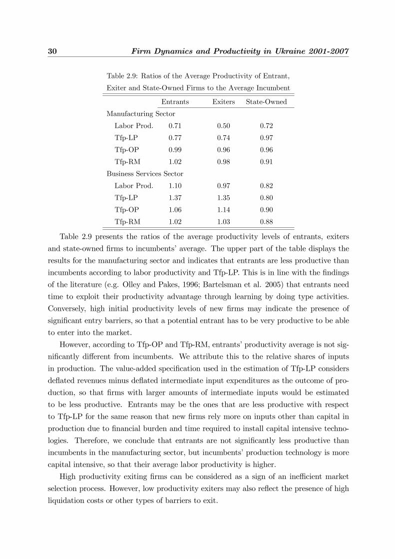
30 Firm Dynamics and Productivity in Ukraine 2001-2007
Table 2.9: Ratios of the Average Productivity of Entrant,
Exiter and State-Owned Firms to the Average Incumbent
Entrants Exiters State-Owned
Manufacturing Sector
Labor Prod. 0.71 0.50 0.72
Tfp-LP 0.77 0.74 0.97
Tfp-OP 0.99 0.96 0.96
Tfp-RM 1.02 0.98 0.91
Business Services Sector
Labor Prod. 1.10 0.97 0.82
Tfp-LP 1.37 1.35 0.80
Tfp-OP 1.06 1.14 0.90
Tfp-RM 1.02 1.03 0.88
Table 2.9 presents the ratios of the average productivity levels of entrants, exiters
and state-owned �rms to incumbents�average. The upper part of the table displays the
results for the manufacturing sector and indicates that entrants are less productive than
incumbents according to labor productivity and Tfp-LP. This is in line with the �ndings
of the literature (e.g. Olley and Pakes, 1996; Bartelsman et al. 2005) that entrants need
time to exploit their productivity advantage through learning by doing type activities.
Conversely, high initial productivity levels of new �rms may indicate the presence of
signi�cant entry barriers, so that a potential entrant has to be very productive to be able
to enter into the market.
However, according to Tfp-OP and Tfp-RM, entrants�productivity average is not sig-
ni�cantly di¤erent from incumbents. We attribute this to the relative shares of inputs
in production. The value-added speci�cation used in the estimation of Tfp-LP considers
de�ated revenues minus de�ated intermediate input expenditures as the outcome of pro-
duction, so that �rms with larger amounts of intermediate inputs would be estimated
to be less productive. Entrants may be the ones that are less productive with respect
to Tfp-LP for the same reason that new �rms rely more on inputs other than capital in
production due to �nancial burden and time required to install capital intensive techno-
logies. Therefore, we conclude that entrants are not signi�cantly less productive than
incumbents in the manufacturing sector, but incumbents�production technology is more
capital intensive, so that their average labor productivity is higher.
High productivity exiting �rms can be considered as a sign of an ine¢ cient market
selection process. However, low productivity exiters may also re�ect the presence of high
liquidation costs or other types of barriers to exit.

2.4 Productivity and Allocative E¢ ciency in Ukraine 31
The second column in Table 2.9 displays the average productivity ratios of exiting to
incumbent �rms. The exiting �rms�average labor productivity is half of the incumbents�
in the manufacturing sector of Ukraine. The exiters have a signi�cantly lower average
productivity with respect to Tfp-LP, but the other two total factor productivity indices
re�ect that exiting establishments�productivity levels are not dramatically lower than
incumbents. The productivity averages based on the four alternative indices di¤er for ex-
iters, possibly because exiting �rms also rely on less capital intensive production methods
as they shrink during the exit phase. It is more probable that exiting �rms do not invest
on capital or compensate the depreciation, once they make the exit decision and enter into
the liquidation phase. However, the intermediate inputs are �exible, and displacement
of existing labor would be less costly, if it is done in the last stage of the exit phase.
Therefore, one may conclude that exiting �rms are not very low or high productive, and
the market selection seems to function e¢ ciently in the manufacturing sector of Ukraine.
The bottom panel of Table 2.9 displays the relative productivity of entrants, exiters
and state-owned �rms in the Ukrainian business services sector. According to all four
measures of productivity, entrant �rms are on average more productive than incumbents.
This is the opposite of what is observed in the manufacturing sector, so that there is
considerable evidence for the presence of substantial entry barriers that allow only the
potentially most productive units to enter into the business services industries.
Exiting �rms are also on average more productive than incumbents according to all
three TFP measures, and exiters�average labor productivity is not signi�cantly di¤erent
from incumbents. Taking into account the fact that the exiting establishments are ex-
pected to be more labor-intensive, one can also argue that the market selection process
does not function e¢ ciently in the business services industries. This may be due to the
presence of signi�cant frictions that weakens the link between e¢ ciency and exit.
Entrants�and exiters�average productivity levels are distinctively large in business
services according to Tfp-LP. This is because of the selection problem mentioned earlier.
Namely, the log transformation of value-added causes a large number of �rms with non-
positive value-added to be eliminated in the estimation sample. Those �rms include a
large portion of low-productivity entrants and exiters in business services, so that the
remaining entrant and exiting �rms�average total factor productivity levels are slightly
overestimated by the LP routine.
According to the last column of Table 2.9, the four productivity measures re�ect that
the state-owned �rms are on average less productive than incumbents in the two main
sectors of Ukraine�s economy. In particular, the labor productivity average of the state-
owned �rms in manufacturing sector is distinctively lower than incumbents. This indicates

32 Firm Dynamics and Productivity in Ukraine 2001-2007
that state-owned �rms operate with larger labor share in production, possibly because
macroeconomic policies that aim to avoid high unemployment rates are involved in the
management strategies of the state-owned establishments.
If we exclude the considerations based on labor productivity, the state-owned establish-
ments seem to have lower relative productivity in business services than in the manufac-
turing sector. Combining this with the previous section�s conclusion that the state-owned
�rms have a larger share in the business services industries, there is also some degree
of evidence that production factors are concentrated in less productive establishments,
so that the factor allocation across �rms is relatively ine¢ cient in the business services
sector.
Table 2.9 provided an intuitive picture of �rms�productivity dynamics in Ukraine. The
next part focuses on the allocative e¢ ciency in the main sectors through a productivity
decomposition method.
2.4.2 Analysis of Allocative E¢ ciency through Olley-Pakes Pro-
ductivity Decomposition
Olley and Pakes (1996) decompose the aggregate (weighted average) productivity into
two components that are the unweighted average productivity and the covariance term
that is referred to the OP-gap.Xsi�i = �� +
X��i � ��
�(si � �s) (2.5)
In equation 2.5, �i represent the �rm speci�c productivity, si is the weight that is the
market share of the �rm, �� =X
�i=n is the unweighted average productivity, n is the
number of �rms and �s = 1=n. Our main concern in this formulation is the last term on
the right hand-side, the OP-gap. By calculating the covariance between the market share
and productivity, we can retrieve an index measuring whether the �rms that have larger
shares in the industry are also more productive. In other words, the OP-gap measures
the static allocative e¢ ciency of an industry for a given time period.
In the calculation of the OP-gap, we consider productivity in logarithms and retrieve
the covariance term annually for each 2-digit industry. In the next step, the OP-gap
is averaged over the industries using the industry shares in the sector total as weights.
Lastly, the calculated annual weighted averages of the OP-gap are further averaged over
time to reach the �nal statistics reported in Table 2.10. The OP-gap measured by labor
productivity covers the period 2001-2007, while the OP-gap based on the TFP indices are
measured for a shorter time period (2004-2007) because of the data limitation mentioned

2.4 Productivity and Allocative E¢ ciency in Ukraine 33
earlier. Moreover, we use �rms�labor shares as the weights for labor productivity based
statistics, while the output shares are used for TFP based OP-gap calculations.10
Table 2.10: Average OP-gap in the Broad Sectors
Labor Prod. Tfp-LP Tfp-OP Tfp-RM
Manufacturing 0.60 0.86 0.22 0.05
Private Sector 0.28 0.58 0.19 0.04
Business Services 0.15 0.64 0.19 0.03
Private Sector 0.37 0.39 0.37 0.06
In Table 2.10, the OP-gap calculations are reported for all �rms and private �rms
separately. When we consider the results for the entire sample, the allocation of �rm
shares within the industries of the manufacturing sector is more e¢ cient than it is for
the business services sector with respect to all four productivity measures. This is in line
with our previous results that production factors are concentrated in relatively ine¢ cient
units in the business services industries.
However, when we exclude the publicly owned establishments, the overall allocative
e¢ ciency in business services dramatically rise according to the OP-gap calculations based
on labor productivity, Tfp-OP and Tfp-RM. This indicates that the �rms that are holding
production factors ine¢ ciently are mostly publicly owned in business services. Further-
more, excluding Tfp-LP, allocative e¢ ciency is higher in the private business services than
in the private manufacturing sector. Therefore, the allocation is relatively e¢ cient in the
private sector of business services, possibly because a large portion of the market share is
held by the state-owned businesses, so that competition among private �rms is intensive.
The reported e¢ ciency in the factor allocation based on Tfp-LP is rather di¤erent
for the business services sector in comparison to those based on other indices. This is
mainly because of the abovementioned selection bias that causes ine¢ cient �rms to be
eliminated in the sample especially in the business services industries. Moreover, although
the story derived from Tfp-OP and labor productivity is also valid for Tfp-RM, the OP-
gap calculations based on Tfp-RM are signi�cantly lower. There are two main reasons for
this. First, the Tfp-RM method adjusts the production function estimates to price-cost
10In the traditional way of calculating the aggregate productivity, �rms�joint input shares are often used
as the weights that is l�itk�it=P
i l�itk
�it in a general Cobb-Douglas type production function speci�cation
with two factors of production. However, the RM method does not estimate the factor elasticities, but
uses the input expenditure shares in the revenues that di¤er for each �rm and time period. Therefore,
in order to produce comparable results across the di¤erent measures of TFP, we use the output shares
as the respective weights, while using the joint input shares does not signi�cantly change our conclusions
based on the Tfp-LP and Tfp-OP indices.

34 Firm Dynamics and Productivity in Ukraine 2001-2007
markups that are generally above one. However, the log productivity index retrieved from
the RM method is divided by a constant markup term that is not possible to disentangle
from the index itself. Thus, the OP-gap calculations based on Tfp-RM are pulled down
by a factor equal to the markup.11 Second, the Tfp-RM routine assumes the markups are
same for all �rms in an industry (in our case its 2-digit industry). This leads �rms having
lower markups than the industry average to be represented less productive, while high-
markup �rms would be measured more productive by RM routine. Therefore, assuming
the correlation between markups and actual productivity is negative (e.g. Foster et al.,
2008), the RM routine shortens the productivity gap between more and less productive
establishments which would, in turn, lower the average OP-gap values in comparison to
the ones based on other productivity indices. Therefore, the OP-gap calculations for a
�rm group based on di¤erent productivity indices are not directly comparable.
2.4.3 Determinants of Productivity
In the previous parts, we discussed various institutional and regulatory factors that are
e¤ective in shaping �rm dynamics in Ukraine. In the last step of the study, we further
investigate the direct role of those factors in the determination of �rm-level productivity
performances.
In the recent empirical literature, there are a number of econometric methods applied
with the aim of assessing the productivity e¤ects of external factors such as the overall
business environment, institutional and regulatory scheme. Among them, regressing a
labor or total factor productivity index on several �rm and aggregate level indicators
by OLS or instrumental variables based econometric techniques constitute a widely used
approach. However, these estimation methodologies often have own shortcomings and
can be improved in the following ways.
As mentioned earlier, �rm-level productivity is an unobserved variable that is often
measured through some other estimation routines or growth accounting methods. There-
fore, an additional step of estimation where the calculated index is regressed on various
explanatory variables decreases the e¢ ciency and introduces additional error into the
estimation procedure. Nickell (1996) overcomes this shortcoming by reducing the es-
timation procedure into a single step. Namely, rather than using a productivity index,
11De�ning �i to be the actual total factor productivity level of �rm i, the RM method retrieves an
index value for �rm i that is log(�i)=�, where � is the markup term. Therefore, the OP-gap based on
Tfp-RM, which isP�
log(�i)� log(��)�(si � �s) =�, is lower than the actual OP-gap. Nevertheless, the
markup term is assumed to be same for all �rms and comparisons across �rm groups within an industry
is not sensitive to the value of �.

2.4 Productivity and Allocative E¢ ciency in Ukraine 35
Nickell de�nes productivity implicitly within a production function speci�cation and in-
troduces the industry and �rm speci�c explanatory variables into the estimation equation.
Nickell further accounts for the possible serial correlation in unobserved productivity by
estimating a dynamic speci�cation of the production function through an instrumental
variables approach where the lags of the dependent and endogenous variables are used as
the instruments.
For reasons discussed earlier, estimating production functions directly by instrumental
variable approaches may be problematic, especially if available instruments consist of
previous periods�inputs and output. Therefore, we introduce a control function approach
into the estimation equation based on Nickell (1996). The way we model the aggregate
production function is similar to Levinsohn and Petrin (2003) and Olley and Pakes (1996).
Moreover, in the application of the estimation routine, we borrowed much from Poi et al.
(2008). The next part brie�y discusses how we formulate the determinants of productivity
equation.
2.4.4 A Control Function Approach
The brief econometric discussion developed in this section relies on two control function
approaches that are Olley and Pakes (OP) (1996) and Levinsohn and Petrin (LP) (2003).
Therefore, similar to the Nickell (1996) formulation, we express a �rm�s production process
by the following system of equations, where the production function has a Cobb-Douglas
form expressed in logs.
qit = �Llit + �
Kkit + �Mmit + �it + "it (2.6)
�it = Xit� + z (�it�1) + eit (2.7)
In equation 2.6, lit, kit and mit represent the production factors, labor, capital and
intermediate inputs respectively, while �i�s are the factor elasticity parameters, and qitis the �rm�s output. Furthermore, �it represents the unobserved productivity that is
observed by the �rm�s manager, and "it is the productivity shock that is fully unobservable
and assumed to be i.i.d. over time.
Equation 2.7 is the unknown Markov process of productivity with a matrix Xit rep-
resenting the control variables level-shifting the Markov process, and � is the coe¢ cient
vector of the control variables. The term z (�) is the unknown function of previous period�sproductivity that is approximated by a polynomial as in the OP and LP approaches.
Similar to the control function approach described in the probit estimation meth-
odology, we consider the intermediate inputs (mit) to be the proxy for the unobserved

36 Firm Dynamics and Productivity in Ukraine 2001-2007
productivity (�it). Assuming that intermediate inputs is a monotonic function of pro-
ductivity, the estimating equation with the control function � (mit; kit) can be written in
the following form.
qit = �Llit + �
Kkit + �Mmit +Xit� + � (mit�1; kit�1) + "it + eit (2.8)
As in the OP and LP routines, we estimate equation 2.8 in two steps, where �L and
� are retrieved in the �rst step. However, since the variables kit and mit appear also
in the control function, the regarding parameters (�K , �M) are identi�ed in the second
step by solving a non-linear least squares problem, and the standard errors are calculated
by block bootstrapping. Following the estimation routine provided by Poi et al. (2008),
we use the Stata�s nl command to solve the non-linear minimization problem. A more
extended formulation of the production function estimation methods used in this chapter
can be found in the appendix.
We avoid using one feature of the OP approach that is the introduction of the exit
probabilities as a state variable into the control function for two main reasons. First,
in the previous parts where we estimate a probit on exit, we �nd that various control
variables representing overall business conditions in an industry do not have explanatory
powers in the business services sector. This indicates that exit is dependent on other
factors such as institutional indicators measuring the regulatory burden over the �rms or
even corruption for which we do not have any additional variables. Second, the structural
model in the OP approach basically assumes productivity to be the main determinant
of �rm exit, but as shown in Table 2.9, the exiters are on average more productive than
incumbents especially in the business services sector. Therefore, the introduction of the
implicit formulation of threshold productivity would not be an empirically consistent
assumption with the observed industry dynamics. Moreover, our results also show that
state-owned �rms have an higher exit rate possibly because of intensive privatization
e¤orts undertaken by the Ukrainian government which further weakens the argument
that �rms exit due to their poor productivity performances.
The matrix X consists of control variables that are de�ned at either the 2-digit
industry- or �rm-level and assumed to be level shifting the Markov process of productivity.

2.4 Productivity and Allocative E¢ ciency in Ukraine 37
Table 2.11: Variables Used in the Estimation of the Production Function
Variables Description
Control variables (Xit)
EntRatejt Ratio of the amount of labor employed by entrants to incumbents.
ExtRatejt Ratio of the amount of labor employed by exiters to incumbents.
PMjt Average variable pro�t to revenue ratio.
Indsizejt Total output produced in industry j in logs.
Ownit Dummy that is equal to 1 for the state-owned �rms.
Sizeit Dummy that is equal to 1 for the �rms with less than 20 emp.
Taxit Ratio of taxes and fees paid by the �rm to total revenues.
t Time trend.
Production Function
qit Output proxied by revenues de�ated by 2-digit industry PPI.
kit Capital input proxied by reported depreciation of the capital stock.
lit Total annual working hours in logs.
mit Intermediate inputs in logs: materials, energy and services realized
without any additional processing at the given �rm.
Table 2.11 displays the variables used in the estimation where the index j re�ects
that the variable is measured at the 2-digit industry-level, and the index i stands for
the �rm speci�c variables. The industry-level employment weighted entry and exit rates
are introduced as explanatory variables. By doing so, we aim to answer whether there
is an ongoing creative destruction process through which the new and potentially more
productive units push out the old and ine¢ cient ones. Thus, if the �rm entry and exit
are due to creative destruction, we would expect the industry-wide entry (EntRatejt)
and exit rates (ExtRatejt) to have signi�cantly positive e¤ects on productivity. In order
to account for possible delays in the entrants productivity growth due to the negative
shocks faced in the start-up phase, the previous period�s entry and exit rates are further
introduced into the estimation equation.
We also consider the pro�t margin (PMjt) as a measure of pro�tability which is also
interpreted as an indicator of the degree of competition in an industry. Therefore, if a
decrease in pro�ts associated with an increase in competition motivates �rms to be more
productive, then one would expect the coe¢ cient estimate to have a negative sign. The
e¤ect of the overall industry on productivity is estimated through the variable Indsizejt.

38 Firm Dynamics and Productivity in Ukraine 2001-2007
Two �rm speci�c dummy variables, Ownit and Sizeit, are introduced into the estim-
ating equation to capture possibly divergent productivity dynamics of the state-owned
and small �rms respectively.
In Ukrainian �rm-level survey, we have a vector of observations described as taxes,
fees (mandatory payments) paid by the �rms. We consider this variable as a measure of
�rm speci�c tax burden and use it in the form of the taxes over revenues ratio (Taxit) in
the estimation equation. We expect the coe¢ cient estimate of the tax to revenue ratio to
measure the impact of �rm speci�c tax intensity on productivity.
Lastly, the capital (kit), labor (lit) and intermediate inputs (mit) are considered as the
factors of production, while intermediate inputs is used also as the proxy variable, and t
is the time trend. We proxy �rm-level output with revenues de�ated by 2-digit industry
PPI. In the appendix, more can be found on the construction of the variables, the method
of price adjustment and the basic statistics on the distribution of the variables used in
this analysis.
Table 2.12 reports the estimation results for the manufacturing and business services
sectors of Ukraine. In order to assess the e¤ects of the variations of overall business
conditions across industry and over time on �rms�productivity performances, we estimate
the production functions at the aggregate (sector) level with 2-digit industry and time
dummies. The industry classi�cation also can be found in the appendix.

2.4 Productivity and Allocative E¢ ciency in Ukraine 39
Table 2.12: Determinants of Productivity
Manufacturing Sector Business Services
Coef Std Coef Std
EntRatejt 1.139** (0.248) 1.343** (0.148)
EntRatejt�1 1.893** (0.193) 0.898** (0.167)
ExtRatejt 2.432** (0.256) �0.077 (0.157)
ExtRatejt�1 2.412** (0.218) 0.022 (0.131)
PMjt �0.851** (0.071) 0.759** (0.066)
Indsizejt 0.099** (0.022) �0.010 (0.007)
Ownit �0.015* (0.008) �0.005 (0.010)
Sizeit �0.011* (0.005) 0.050** (0.005)
Taxit �0.318** (0.085) �0.837** (0.010)
t 0.070** (0.007) �0.089** (0.004)
kit 0.146** (0.020) 0.191** (0.020)
lit 0.270** (0.003) 0.321** (0.003)
mit 0.427** (0.084) 0.278** (0.084)
#obs 105894 308434
**Signi�cant at 1%. *Signi�cant at 5%.
Time and industry dummies are included.
According to the left hand-side of Table 2.12, the current and previous periods�entry
rates signi�cantly a¤ect productivity in the manufacturing industries of Ukraine. The
coe¢ cient estimate of the previous period�s entry rate is larger with a lower standard
error in comparison to today�s entry rate. We attribute this to entrants�poor productivity
performances in the �rst year in the manufacturing sector. Therefore, entrants become
more serious competitors of incumbents after the start-up phase, and motivate other �rms
to be more productive with a lag.
Even though we partially control for the e¤ects of the overall level of competition on
productivity through the pro�t margin, the positive e¤ect of entry on productivity is still
signi�cant. One may argue that the positive relation between entry rate and productivity
is due to highly productive entrants, but as shown in the previous parts, entrants are
not more productive than incumbents in the manufacturing industries according to four
alternative measures of �rm-level productivity. Therefore, the entry of new �rms pos-
itively in�uences incumbents productivity performances possibly through channels like
technological di¤usion and more intense competition.

40 Firm Dynamics and Productivity in Ukraine 2001-2007
The current and previous periods�exit rates have signi�cantly positive e¤ects on �rm-
level productivity dynamics. This is mainly because the exit of ine¢ cient units releases
a portion of production factors, which can be re-combined in more e¢ cient units and
facilitate productivity growth. A joint interpretation of the coe¢ cient estimates of entry
and exit rates further shows that creative destruction functions e¢ ciently in the manu-
facturing industries, so that there are signi�cant productivity gains from both entry and
exit simultaneously.
The degree of competition represented by the pro�t margin (PMjt) has a signi�cant
productivity enhancing e¤ect. The overall increase in competition motivates �rms to be
more productive, which may mean that escape from competition e¤ect is dominant in the
manufacturing sector of Ukraine. It is also possible to argue that productivity plays a role
in the determination of the pro�ts of an industry, but as Nickell (1996) argues, possible
endogeneity of pro�ts to productivity would lead to retrieve a positive coe¢ cient estimate
for the pro�t margin. However, the estimated coe¢ cient is signi�cantly negative, so that
if there is an endogeneity problem even after controlling for unobserved productivity, the
actual negative relationship between the pro�t margin and productivity is even stronger
than what we estimate.
We introduce the variable Indsizejt to control for overall size e¤ects on productivity,
so that coe¢ cients retrieved from other industry level variables such as PMjt are not
sensitive to industry size. The parameter estimate of the industry size is positive and
signi�cant indicating that overall size play a role in the determination of manufacturing
�rms�productivity dynamics. This may be because, for instance, the degree of openness
of an industry to trade a¤ects both industry size and productivity in the same way.
The ownership dummy has a negative coe¢ cient estimate that is signi�cant only at
the 5% level. This is in line with the results displayed in Table 2.9 that the average
productivity of state-owned �rms is slightly lower than incumbents�average. Moreover,
size dummy (Sizeit) representing small �rms has a signi�cantly (at 5%) negative coe¢ cient
indicating that the factor allocation is e¢ cient in the manufacturing sector.
The variable Taxit that represents �rm speci�c tax to revenue ratio has a signi�cantly
negative e¤ect on productivity. Namely, our results show that the tax burden in the man-
ufacturing sector is still e¤ective enough to deteriorate �rms�productivity performance,
despite recent e¤orts to decrease the regulatory burden on �rm activities.
The productivity dynamics in the business services sector of Ukraine have rather
di¤erent features in comparison to the observed dynamics in the manufacturing sector.
According to the right hand-side of Table 2.12, the current and previous periods�entry
rates are signi�cantly and positively a¤ecting �rm-level productivity performances. This

2.4 Productivity and Allocative E¢ ciency in Ukraine 41
is in line with our expectations, since in the previous parts, we already concluded that
entrants were on average much more productive than incumbents in business services.
The coe¢ cient of the current period�s entry rate is relatively large indicating that business
services producing �rms start up rather e¢ ciently. However, the e¤ect of the previous
period�s entry rate on productivity is estimated to be lower than the current entry rate.
Therefore, our results imply that the post-entry productivity improvement is relatively
slow in the business services sector.
In contrast to the manufacturing sector, the variables representing the current and
lagged exit rates do not have any explanatory power on productivity dynamics in the
business services industries of Ukraine with the current period�s exit rate having a negative
parameter estimate. This further emphasize that the exit process is rather ine¢ cient, and
there are no signi�cant productivity gains from exit in business services. Combining
this with the previous �ndings that exiters are more productive than incumbents in the
business services industries, the resulting �rm destruction seems to have dynamics which
are di¤erent from what one expects to observe in a healthy functioning market.
The pro�t margin has a positive coe¢ cient estimate, so that competition has a sig-
ni�cantly negative e¤ect on �rm-level productivity performance in the business services
sector. Therefore, rather than escaping from competition, being pro�table is the main
driving force of business services producing �rms to engage in productivity enhancing
activities. This may be due to relatively low level of competition among �rms.
The observed link between competition and productivity in the business services sector
is in line with the Schumpeterian view, namely as the monopolistic powers are large in
an industry, �rms tend to invest more in R&D type innovative activities. In addition,
the variable representing industry size (Indsizejt) has an insigni�cant coe¢ cient estimate
indicating that the business services industries expand or shrink regardless of productivity
related external factors.
The dummy variable (Ownit) that stands for the state-owned �rms has a negative
but insigni�cant coe¢ cient estimate. This is consistent with what we observed in the
descriptive part, so that in business services, large �rms are ine¢ cient regardless of the
ownership structure. However, state-ownership dominates the business services sector,
and the observed dynamics in business services such as, ine¢ cient factor allocation, un-
favorable entry and exit conditions are signi�cantly related with the large share of public
ownership.
The dummy variable for small enterprises in the business services has a signi�cantly
positive coe¢ cient estimate. This is also in line with previous conclusions that small-sized
private establishments constitute the most productive �rm group in the business services.

42 Firm Dynamics and Productivity in Ukraine 2001-2007
Therefore, one can conclude that the reallocation of the production factors from the state-
owned establishments to the small-sized private enterprises and potential entrants would
signi�cantly increase the sector�s productivity performance.
The tax intensity (Taxit) has a signi�cantly negative coe¢ cient estimate that is higher
in absolute value than the estimate retrieved in the manufacturing sector. Therefore,
there is some degree of evidence that the tax burden hinders establishments�productivity
performances.
Lastly, we �nd overall decreasing returns to scale in the manufacturing and business
services sectors. However, in the appendix part, returns to scale estimations with al-
ternative methods are reported at the 2-digit industry-level for all manufacturing and
business services industries, which would provide more detailed and reliable information
on the returns to scale in production in Ukraine.
2.5 Conclusion
In spite of implementing successful reforms towards integrating domestic industries with
the global markets, Ukraine is rather slow in microeconomic restructuring of the business
environment. In particular, the existence of ine¢ ciently large �rms that are mostly state-
owned and operate without incentives to be more productive stays as a persistent problem.
In this respect, our study devotes particular attention to the role of state ownership in the
economy and its e¤ectiveness in shaping �rm dynamics, factor allocation and productivity
in Ukraine.
One of the main �ndings of this chapter is the di¤erences in �rm dynamics between
the manufacturing and business services sectors. The ine¢ ciently large �rms, which
includes a major portion of state-owned establishments as well as private �rms, dominate
the business services industries. Besides distorting factor allocation mechanism through
holding a great portion of the production factors ine¢ ciently, state-owned �rms in business
services signi�cantly constrain aggregate productivity performance.
In the presence of a well-functioning market selection mechanism, one would expect
creative destruction to play an important role in the restructuring of economy by replacing
ine¢ cient units with more e¢ cient ones. We assess the quality of the creative destruction
process through a probit on �rm-level exit, where the industry-level entry rate is intro-
duced as explanatory variables. We �nd either negative or no entry e¤ect on �rm-level
exit in business services industries. In addition, the overall level of competition has an
insigni�cant e¤ect on �rms�exit decisions, indicating that there are other possible factors
such as frictions shaping �rm-survival in business services.

2.5 Conclusion 43
Conversely, creative destruction and competition play signi�cant roles in the Ukrainian
manufacturing sector. The share of state-ownership is relatively low, and the entry of new
production units constitute a signi�cant competitive pressure on incumbents and facilitate
the exit of ine¢ cient �rms in the manufacturing industries. Moreover, large enterprises
also have a dominant share in the manufacturing sector, but evidence provided in this
study shows that those �rms are on average more productive and not ine¢ ciently large
in comparison to large establishments in the business services industries.
In the analysis of �rm-level productivity, we utilize a labor productivity index as well
as three alternative TFP estimation routines with the aim of accounting for possible bias
due to imperfect competition and unobserved �rm-level variation in factor elasticities,
and used alternative variables to proxy unobserved productivity such as investments,
intermediate inputs and variable pro�ts, but the overall results on productivity dynamics
in Ukraine are not really sensitive to alternative measurement methods.
The analysis of productivity also depicts two dramatically di¤erent pictures for the
manufacturing and business services sectors of Ukraine. Therefore, in business services,
exiting �rms are on average at least as productive as incumbents, while potential entrants
need to have very high productivity levels to enter into the market. Due to the existence of
ine¢ ciently large enterprises that are mostly state-owned in the business services sector,
factor allocation is not as e¢ cient as it is in the manufacturing industries.
In the �nal section of this chapter, we applied an aggregate production function es-
timation routine in order to assess the e¤ects of overall business environment on �rms�
productivity performances. We �nd that the current and previous periods� exit rates
have either insigni�cant or negative e¤ects on productivity performance in the business
services, indicating that market selection mechanism does not lead to productivity growth.
Moreover, the �rm speci�c tax burden has a negative e¤ect on �rm-level productivity, and
the e¤ect is stronger for establishments operating in the business services industries.
The industry-level entry and exit signi�cantly alter �rms�productivity dynamics in
the manufacturing sector, so that higher productivity performances are associated with
higher entry and exit rates. While this shows that creative destruction process is well-
functioning in the manufacturing sector, most of the productivity gains from entry of new
producers are realized only one year after the time of entry. We interpret this one-year
delayed entry e¤ect as an expected outcome, because manufacturing �rms may need time
to exploit their productivity advantage due to relatively high capital installation costs,
sunk commitments and possible �nancial constraints faced in the start-up phase.
A policy conclusion is that, signi�cant productivity gains may be expected from privat-
ization especially in the business services industries. In addition to this, regulatory bur-

44 Firm Dynamics and Productivity in Ukraine 2001-2007
den is rather heavy both in terms of taxes and other legal obligations that create barriers
to entry, exit and �rm development. In particular, much of the production factors are
employed in ine¢ cient units, indicating policies that facilitate exit would increase the
productivity growth through factor reallocation in business services. Conversely, ongo-
ing microeconomic restructuring accelerates productivity growth in the manufacturing
sector. Besides it is necessary to keep the favorable business environment stable in the
future periods, in the manufacturing sector, there are few things to do to remove barriers
to not only entry but also �rm development and exit.
2.5.1 Discussions
Throughout the analysis of �rm-level productivity, we proxy the quantity of output with
revenues de�ated by a constructed price index that is based on PPI at 2-digit industry level
for the manufacturing industries and mostly 1-digit industry level PPI for the business
services. The pricing method, which is discussed in the appendix, also takes into account
multi-product �rms, so that the index values vary at the establishment level.
In the measurement of productivity, recent empirical literature particularly emphasizes
the importance of �rm-level price variation (Levinsohn and Melitz, 2004; Foster et al.,
2008). However, as is the case for the dataset used in this study, mostly, prices are
unobservable at the �rm-level. We attempt to control for the unobserved price variation
up to the degree of constant markup that varies across the 2-digit industries by introducing
the production function estimation routine in Martin (2005). However, this may also be
insu¢ cient, if the analysis is carried out beyond the borders of aggregate productivity
growth at the sector or economy level.
Therefore, if the aim is to consider the productivity dynamics of a particular group
within a narrowly de�ned industry, one needs to also take into account the possible
markup variation of this group from the industry average. For instance, as it is empirically
supported in Foster et al., (2008), the group of entrant �rms may su¤er from idiosyncratic
demand shocks in the start-up phase that would restrict their pricing behavior and pull
down the price-cost markups of the entrants. Thus, if one aims to adjust the productivity
index through a constant industry markup, the productivity performance of low markup
�rms such as entrants would be underestimated. However, this would not constitute a
big issue for our conclusions regarding the entrants�productivity performance, since we
already argue that the problem in Ukraine�s business services sectors is that entrants are
on average much more productive than the incumbents. We consider this as a problem,
because it implies that there are signi�cant entry barriers, so that average entrant needs

2.6 Appendix 45
to be highly productive to enter into the market. In case the entrants indeed have lower
markups in our sample, the implications on the entry barriers would be even stronger.
While a similar story would be valid for the exiting �rms, it is hard to predict the markup
dynamics of the group of state-owned �rms, since the state-owned establishments may
operate as non-pro�t organizations and charge lower prices, but they also have signi�cant
market power.
2.6 Appendix
Calculation of the Price Indices for the Missing Industries
The approach used in the calculation of the disaggregated output price indices relies on
Laspyres index that is given by the below formula.
PtP0=
Pi pitqi0P
i pi0qi0
=X
iwi0pitpi0
(A.1)
In the above formula, Pt represents the aggregate price index (sector level PPI) at time
t, where qit and pit is the disaggregated quantity and price indices (2-digit industry level)
at industry i and time t. Moreover, wi0 = pi0qi0=P
j pj0qj0 stands for sector i�s nominal
output share in total, and time 0 is the base time point of the de�ator, while t is the time
period for which it is aimed to obtain a price de�ator.
Therefore, when the price indices of a parent (Pt=P0) and at least one child industry
(pit=pi0) are available, one can calculate a single disaggregated price index for all other
child industries, which are at the same level of the industry classi�cation hierarchy, with
the child industry whose price index is available. Therefore, assuming i 2 A is the indexof the industries whose price indices are available, and j 2 N representing the ones with
missing prices (A\N = ?), a single price index (PNt =PN0 ) for the industries in set N can
be retrieved as follows.
PNtPN0
=X
jwj0pjt
pj0=PtP0�X
iwi0pitpi0
(A.2)
It is also worth noting that when we construct 1-digit industry level PPI�s, we use the
GDP de�ator as the parent�s (in this case it is the total economy) price index.
Calculation of the Firm-Level Price Indices
In Ukrainian �rm-level dataset, there are multi-product �rms that are simultaneously
operating in more than one industry, and the revenues are categorized according to the
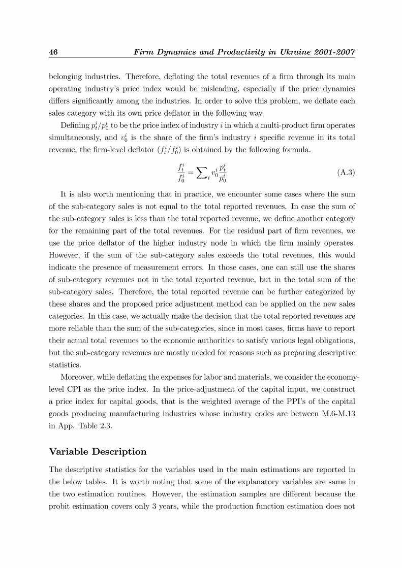
46 Firm Dynamics and Productivity in Ukraine 2001-2007
belonging industries. Therefore, de�ating the total revenues of a �rm through its main
operating industry�s price index would be misleading, especially if the price dynamics
di¤ers signi�cantly among the industries. In order to solve this problem, we de�ate each
sales category with its own price de�ator in the following way.
De�ning pit=pi0 to be the price index of industry i in which a multi-product �rm operates
simultaneously, and vi0 is the share of the �rm�s industry i speci�c revenue in its total
revenue, the �rm-level de�ator (f it=fi0) is obtained by the following formula.
f itf i0=X
ivi0pitpi0
(A.3)
It is also worth mentioning that in practice, we encounter some cases where the sum
of the sub-category sales is not equal to the total reported revenues. In case the sum of
the sub-category sales is less than the total reported revenue, we de�ne another category
for the remaining part of the total revenues. For the residual part of �rm revenues, we
use the price de�ator of the higher industry node in which the �rm mainly operates.
However, if the sum of the sub-category sales exceeds the total revenues, this would
indicate the presence of measurement errors. In those cases, one can still use the shares
of sub-category revenues not in the total reported revenue, but in the total sum of the
sub-category sales. Therefore, the total reported revenue can be further categorized by
these shares and the proposed price adjustment method can be applied on the new sales
categories. In this case, we actually make the decision that the total reported revenues are
more reliable than the sum of the sub-categories, since in most cases, �rms have to report
their actual total revenues to the economic authorities to satisfy various legal obligations,
but the sub-category revenues are mostly needed for reasons such as preparing descriptive
statistics.
Moreover, while de�ating the expenses for labor and materials, we consider the economy-
level CPI as the price index. In the price-adjustment of the capital input, we construct
a price index for capital goods, that is the weighted average of the PPI�s of the capital
goods producing manufacturing industries whose industry codes are between M.6-M.13
in App. Table 2.3.
Variable Description
The descriptive statistics for the variables used in the main estimations are reported in
the below tables. It is worth noting that some of the explanatory variables are same in
the two estimation routines. However, the estimation samples are di¤erent because the
probit estimation covers only 3 years, while the production function estimation does not

2.6 Appendix 47
consider one-year �rms, because of the assumed Markov process for productivity that
requires at least 2 time observations for each �rm. Therefore, the summary statistics for
the same variable used in two di¤erent estimation routines slightly di¤er.
App. Table 2.1: Variables Used in the Probit Estimation
Mean Std. Err. Upper Q. Median Lower Q.
Manufacturing Sector
EntRatejt 0.02 0.01 0.02 0.01 0.01
EntRatejt�1 0.02 0.01 0.03 0.02 0.01
PMjt 0.21 0.04 0.23 0.20 0.17
�Outputjt 0.21 0.15 0.28 0.19 0.14
empit 2.84 1.54 3.74 2.64 1.79
�it 0.25 0.46 0.41 0.23 0.09
kit 4.57 2.31 6.08 4.43 2.96
mit 5.44 2.55 7.13 5.39 3.71
Business Services
EntRatejt 0.04 0.02 0.05 0.04 0.02
EntRatejt�1 0.04 0.02 0.06 0.04 0.03
PMjt 0.21 0.17 0.36 0.10 0.07
�Outputjt 0.23 0.22 0.37 0.25 0.10
empit 2.01 1.24 2.71 1.95 1.10
�it 0.33 0.66 0.43 0.14 0.05
kit 3.70 2.04 5.01 3.59 2.30
mit 5.23 2.70 7.06 5.38 3.51

48 Firm Dynamics and Productivity in Ukraine 2001-2007
App. Table 2.2: Variables in Determinants of Productivity Est.
Mean Std. Err. Upper Q. Median Lower Q.
Manufacturing Sector
qit 6.28 2.12 7.64 6.11 4.81
EntRatejt 0.01 0.01 0.02 0.01 0.01
EntRatejt�1 0.02 0.01 0.03 0.02 0.01
ExtRatejt 0.01 0.01 0.02 0.01 0.01
ExtRatejt�1 0.02 0.01 0.02 0.01 0.01
PMjt 0.21 0.03 0.24 0.20 0.19
Indsizejt 16.64 1.60 17.76 16.63 15.83
Taxit 0.03 0.16 0.04 0.00 0.00
mit 5.71 2.41 7.30 5.60 4.04
kit 4.68 2.31 6.20 4.55 3.08
lit 10.34 1.60 11.27 10.20 9.29
Business Services
qit 6.01 2.02 7.29 5.90 4.62
EntRatejt 0.03 0.03 0.04 0.03 0.02
EntRatejt�1 0.04 0.02 0.06 0.04 0.03
ExtRatejt 0.03 0.01 0.03 0.03 0.02
ExtRatejt�1 0.03 0.02 0.04 0.03 0.02
PMjt 0.24 0.19 0.41 0.11 0.09
Indsizejt 16.63 1.53 18.07 16.83 15.37
Taxit 0.03 0.11 0.03 0.00 0.00
mit 5.36 2.66 7.14 5.48 3.66
kit 3.76 2.06 5.09 3.65 2.36
lit 9.53 1.33 10.30 9.42 8.70
Production Function Estimations
Below parts provide a brief description of the production function estimations used in this
study. Therefore, we start with Levinsohn and Petrin (2003) (LP) approach, and discuss
the di¤erences of Olley and Pakes (1996) (OP) and Martin (2005) (RM) from the LP.
Levinsohn and Petrin (2003) approach

2.6 Appendix 49
Assuming a Cobb-Douglas type functional form, the value added (vit) speci�cation of
the logged production function can be written as follows.
vit = �Llit + �
Kkit + � (mit; kit) + "it (A.4)
Therefore, lit and kit stand for the labor and capital inputs wheremit is the proxy vari-
able that is the intermediate inputs in the LP. Moreover, in equation A.4, �it (�) =M�1it (�)
is the control function in an unknown form. However, it is not possible to identify the
coe¢ cient of the capital input separately from the non-parametric part of the estimation
� (mit; kit) in a single step. Therefore, the standard approach requires two steps, so that
in the �rst step, we de�ne a non-parametric function g (mit; kit) which is represented by a
high order polynomial (3rd order in Levinsohn et al., 2004) in its arguments and captures
the unobserved productivity and the state variable capital jointly. Assuming lit is the
variable factor of production, the identi�cation of the coe¢ cient of the variable factor
(�L) is feasible in the �rst step. The �rst stage regression equation can be written as
follows.
vit = �Llit + g (mit; kit) + "it (A.5)
g (mit; kit) = �Kkit + � (mit; kit) (A.6)
Estimation of A.5 by OLS provides the coe¢ cient estimate �L. Additionally, we can
retrieve an estimate of the function g (mit; kit) which is used to express the unobserved
productivity for given parameter value of �K that will be further identi�ed in the last
step of the estimation routine.
�it = g (mit; kit)� �K�kit (A.7)
Assuming the productivity to follow a �rst order Markov process, the evaluation of
�rm-level productivity can be written in the polynomial speci�cation as follows.
�it = 0 + 1�it�1 + 2�2
it�1 + eit (A.8)
Accordingly, for given �K�, one can run the above regression where the �tted values is
used as an estimate for the expectation of productivity conditional on previous period�s
productivity realization E \(�it j �it�1) = h(�it�1) . Therefore, joint minimization of the
error terms ("it + eit) with respect to �K would provide an estimate of the coe¢ cient of
capital.
min�K
h"it + eit = vit � �Llit �Xit� � �K�kit � h(�it�1)
i(A.9)
The equation A.9 represents the �nal equation of the estimation routine, and all the
respective coe¢ cients are identi�ed at the end of the second step. Following the Stata
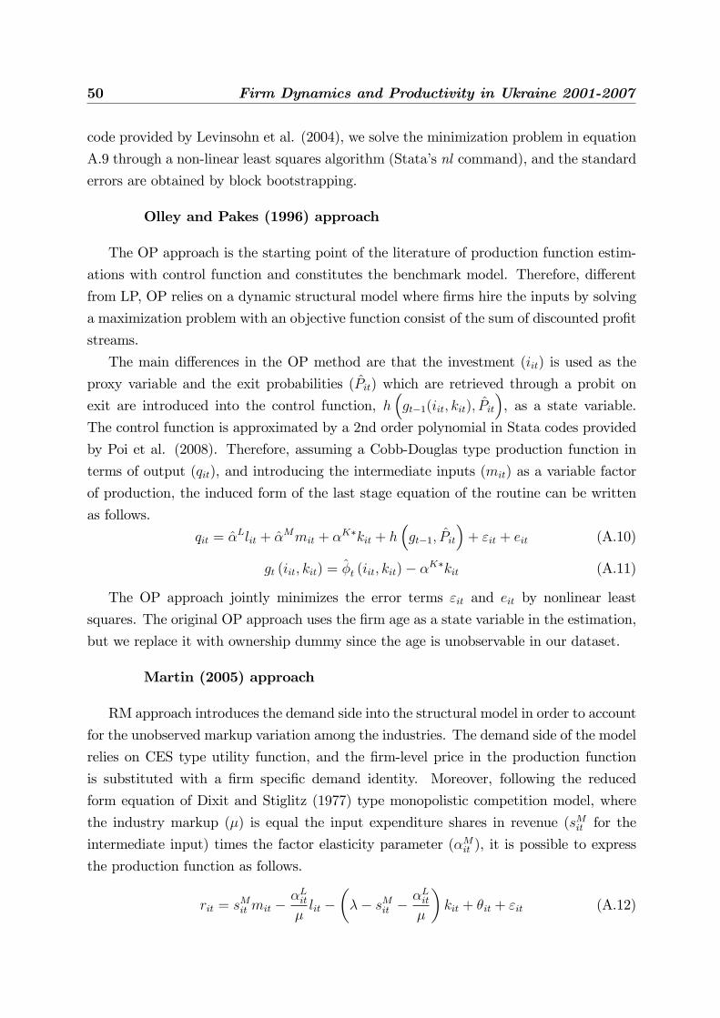
50 Firm Dynamics and Productivity in Ukraine 2001-2007
code provided by Levinsohn et al. (2004), we solve the minimization problem in equation
A.9 through a non-linear least squares algorithm (Stata�s nl command), and the standard
errors are obtained by block bootstrapping.
Olley and Pakes (1996) approach
The OP approach is the starting point of the literature of production function estim-
ations with control function and constitutes the benchmark model. Therefore, di¤erent
from LP, OP relies on a dynamic structural model where �rms hire the inputs by solving
a maximization problem with an objective function consist of the sum of discounted pro�t
streams.
The main di¤erences in the OP method are that the investment (iit) is used as the
proxy variable and the exit probabilities (Pit) which are retrieved through a probit on
exit are introduced into the control function, h�gt�1(iit; kit); Pit
�, as a state variable.
The control function is approximated by a 2nd order polynomial in Stata codes provided
by Poi et al. (2008). Therefore, assuming a Cobb-Douglas type production function in
terms of output (qit), and introducing the intermediate inputs (mit) as a variable factor
of production, the induced form of the last stage equation of the routine can be written
as follows.
qit = �Llit + �
Mmit + �K�kit + h
�gt�1; Pit
�+ "it + eit (A.10)
gt (iit; kit) = �t (iit; kit)� �K�kit (A.11)
The OP approach jointly minimizes the error terms "it and eit by nonlinear least
squares. The original OP approach uses the �rm age as a state variable in the estimation,
but we replace it with ownership dummy since the age is unobservable in our dataset.
Martin (2005) approach
RM approach introduces the demand side into the structural model in order to account
for the unobserved markup variation among the industries. The demand side of the model
relies on CES type utility function, and the �rm-level price in the production function
is substituted with a �rm speci�c demand identity. Moreover, following the reduced
form equation of Dixit and Stiglitz (1977) type monopolistic competition model, where
the industry markup (�) is equal the input expenditure shares in revenue (sMit for the
intermediate input) times the factor elasticity parameter (�Mit ), it is possible to express
the production function as follows.
rit = sMit mit �
�Lit�lit �
��� sMit �
�Lit�
�kit + �it + "it (A.12)
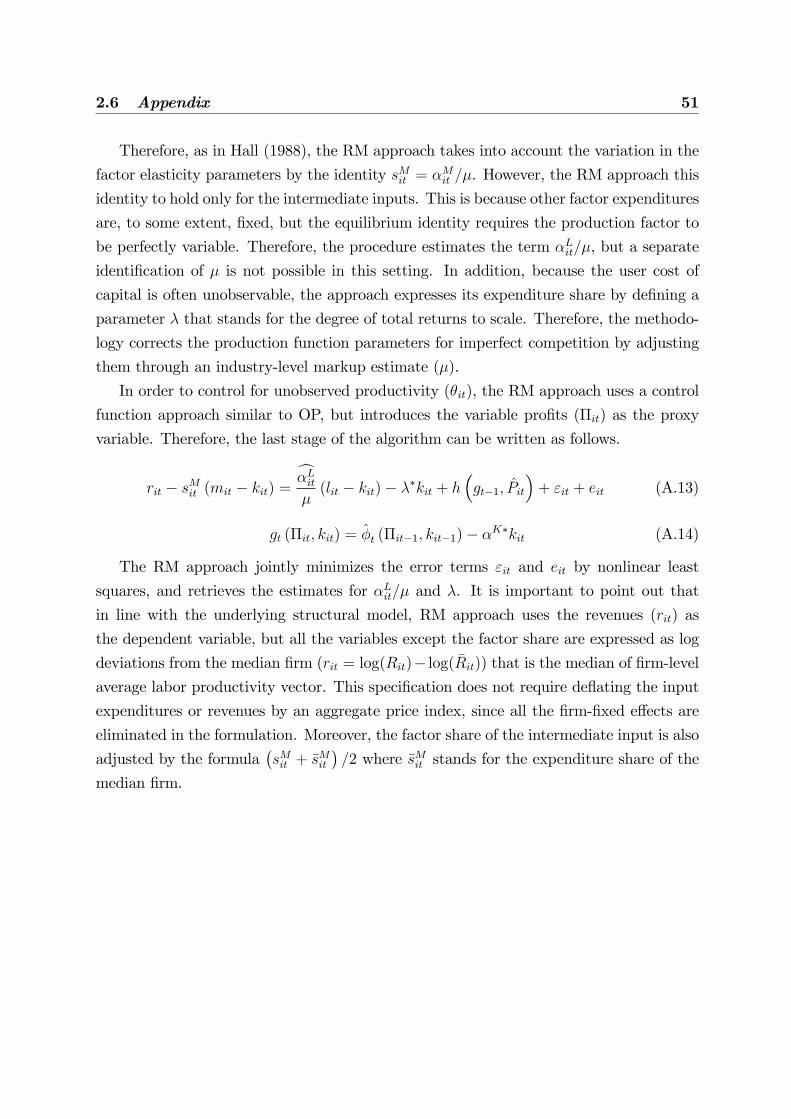
2.6 Appendix 51
Therefore, as in Hall (1988), the RM approach takes into account the variation in the
factor elasticity parameters by the identity sMit = �Mit =�. However, the RM approach this
identity to hold only for the intermediate inputs. This is because other factor expenditures
are, to some extent, �xed, but the equilibrium identity requires the production factor to
be perfectly variable. Therefore, the procedure estimates the term �Lit=�, but a separate
identi�cation of � is not possible in this setting. In addition, because the user cost of
capital is often unobservable, the approach expresses its expenditure share by de�ning a
parameter � that stands for the degree of total returns to scale. Therefore, the methodo-
logy corrects the production function parameters for imperfect competition by adjusting
them through an industry-level markup estimate (�).
In order to control for unobserved productivity (�it), the RM approach uses a control
function approach similar to OP, but introduces the variable pro�ts (�it) as the proxy
variable. Therefore, the last stage of the algorithm can be written as follows.
rit � sMit (mit � kit) =c�Lit�(lit � kit)� ��kit + h
�gt�1; Pit
�+ "it + eit (A.13)
gt (�it; kit) = �t (�it�1; kit�1)� �K�kit (A.14)
The RM approach jointly minimizes the error terms "it and eit by nonlinear least
squares, and retrieves the estimates for �Lit=� and �. It is important to point out that
in line with the underlying structural model, RM approach uses the revenues (rit) as
the dependent variable, but all the variables except the factor share are expressed as log
deviations from the median �rm (rit = log(Rit)� log( �Rit)) that is the median of �rm-levelaverage labor productivity vector. This speci�cation does not require de�ating the input
expenditures or revenues by an aggregate price index, since all the �rm-�xed e¤ects are
eliminated in the formulation. Moreover, the factor share of the intermediate input is also
adjusted by the formula�sMit + �s
Mit
�=2 where �sMit stands for the expenditure share of the
median �rm.
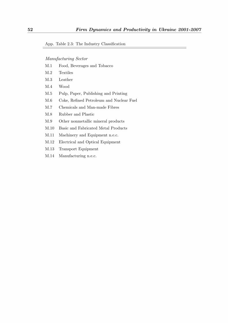
52 Firm Dynamics and Productivity in Ukraine 2001-2007
App. Table 2.3: The Industry Classi�cation
Manufacturing Sector
M.1 Food, Beverages and Tobacco
M.2 Textiles
M.3 Leather
M.4 Wood
M.5 Pulp, Paper, Publishing and Printing
M.6 Coke, Re�ned Petroleum and Nuclear Fuel
M.7 Chemicals and Man-made Fibres
M.8 Rubber and Plastic
M.9 Other nonmetallic mineral products
M.10 Basic and Fabricated Metal Products
M.11 Machinery and Equipment n.e.c.
M.12 Electrical and Optical Equipment
M.13 Transport Equipment
M.14 Manufacturing n.e.c.

2.6 Appendix 53
Business Services Sector
B.1 Sale, maintenance and repair of motor vehicles and motorcycles
B.2 Wholesale on a fee or contract basis
B.3 Wholesale of agricultural raw materials and live animals
B.4 Wholesale of food, beverages and tobacco
B.5 Wholesale of household goods
B.6 Wholesale of non-agricultural intermediate products, waste, scrap
B.7 Wholesale of machinery, equipment and supplies, other wholesale
B.8 Retail sale of food, beverages and tobacco in specialized stores
B.9 Other retail sale of food, beverages and tobacco in specialized stores
B.10 Repair of personal and household goods, Retail not in stores
B.11 Other wholesale
B.12 Retail sale in non-specialized stores
B.13 Retail sale of pharmaceutical and medical goods, cosmetic articles
B.14 Hotels and restaurants
B.15 Transport
B.16 Post and telecommunications
B.17 Financial intermediation
B.18 Renting of machinery, equipment, personal and household goods
B.19 Computer and related activities
B.20 Research and development
B.21 Legal activities
B.22 Accounting, book-keeping and auditing activities
B.23 Business and management consultancy activities
B.24 Architectural and engineering activities
B.25 Technical testing and analysis, advertising, labour recruitment
B.26 Investigation and security activities, Industrial cleaning
B.27 Miscellaneous business activities n.e.c.

54 Firm Dynamics and Productivity in Ukraine 2001-2007
App. Table 2.4: Production Function Estimation Results (1)
LP OP RM
Labor Capital Labor Capital Materials Labor RTS
M.1 0.502 0.281 0.134 0.059 0.789 0.152 0.976
(0.014) (0.016) (0.005) (0.012) (0.005) (0.018) (0.017)
M.2 0.705 0.147 0.444 0.057 0.481 0.400 0.957
(0.017) (0.020) (0.013) (0.012) (0.009) (0.025) (0.024)
M.3 0.627 0.149 0.364 0.080 0.571 0.204 0.910
(0.037) (0.070) (0.028) (0.032) (0.025) (0.056) (0.056)
M.4 0.641 0.169 0.269 0.037 0.653 0.273 0.971
(0.022) (0.018) (0.010) (0.017) (0.008) (0.022) (0.023)
M.5 0.512 0.200 0.283 0.097 0.606 0.309 0.953
(0.014) (0.010) (0.008) (0.009) (0.008) (0.017) (0.020)
M.6 0.520 0.367 0.042 0.069 0.819 0.096 1.020
(0.325) (0.298) (0.034) (0.047) (0.032) (0.093) (0.100)
M.7 0.528 0.399 0.153 0.069 0.733 0.195 0.988
(0.040) (0.060) (0.012) (0.016) (0.016) (0.041) (0.046)
M.8 0.509 0.284 0.166 0.056 0.751 0.234 0.991
(0.032) (0.034) (0.010) (0.010) (0.010) (0.080) (0.075)
M.9 0.615 0.258 0.218 0.058 0.708 0.274 0.991
(0.025) (0.041) (0.010) (0.017) (0.008) (0.025) (0.027)
M.10 0.633 0.317 0.191 0.074 0.738 0.249 0.998
(0.028) (0.033) (0.007) (0.010) (0.006) (0.021) (0.022)
M.11 0.618 0.219 0.260 0.072 0.658 0.309 1.007
(0.018) (0.019) (0.009) (0.010) (0.007) (0.051) (0.050)
M.12 0.537 0.248 0.225 0.127 0.644 0.274 0.995
(0.017) (0.023) (0.011) (0.012) (0.009) (0.031) (0.031)
M.13 0.612 0.258 0.294 0.114 0.581 0.270 0.960
(0.019) (0.025) (0.015) (0.016) (0.013) (0.029) (0.028)
M.14 0.631 0.228 0.206 0.039 0.744 0.138 0.883
(0.030) (0.050) (0.009) (0.013) (0.007) (0.031) (0.027)
Standard errors are in parenthesis.

2.6 Appendix 55
App. Table 2.5: Production Function Estimation Results (2)
LP OP RM
Labor Capital Labor Capital Materials Labor RTS
B.1 0.704 0.361 0.169 0.095 0.768 0.180 1.036
(0.023) (0.033) (0.006) (0.008) (0.005) (0.010) (0.009)
B.2 0.661 0.255 0.253 0.145 0.589 0.263 0.999
(0.028) (0.047) (0.010) (0.023) (0.008) (0.031) (0.034)
B.3 0.381 0.364 0.073 0.018 0.924 0.097 0.996
(0.038) (0.105) (0.004) (0.008) (0.003) (0.010) (0.008)
B.4 0.285 0.346 0.043 0.032 0.929 0.070 1.001
(0.031) (0.054) (0.003) (0.007) (0.003) (0.005) (0.005)
B.5 0.360 0.261 0.070 0.040 0.904 0.128 1.011
(0.028) (0.044) (0.004) (0.005) (0.004) (0.006) (0.007)
B.6 0.279 0.316 0.048 0.018 0.933 0.093 1.014
(0.019) (0.062) (0.002) (0.005) (0.002) (0.004) (0.004)
B.7 0.343 0.441 0.062 0.029 0.918 0.089 0.997
(0.035) (0.112) (0.004) (0.003) (0.004) (0.007) (0.006)
B.8 0.702 0.162 0.137 0.032 0.835 0.136 0.981
(0.070) (0.159) (0.013) (0.013) (0.015) (0.025) (0.022)
B.9 0.579 0.230 0.144 0.058 0.816 0.172 0.979
(0.039) (0.049) (0.007) (0.008) (0.008) (0.015) (0.013)
B.10 0.838 0.147 0.453 0.086 0.499 0.586 0.989
(0.026) (0.032) (0.021) (0.017) (0.012) (0.060) (0.067)
B.11 0.389 0.289 0.065 0.035 0.916 0.095 1.006
(0.016) (0.024) (0.001) (0.003) (0.002) (0.003) (0.003)
B.12 0.565 0.182 0.112 0.050 0.840 0.132 0.981
(0.022) (0.034) (0.004) (0.004) (0.004) (0.004) (0.004)
B.13 0.453 0.164 0.091 0.029 0.884 0.150 0.984
(0.038) (0.094) (0.004) (0.005) (0.005) (0.008) (0.008)
Standard errors are in parenthesis.

56 Firm Dynamics and Productivity in Ukraine 2001-2007
App. Table 2.6: Production Function Estimation Results (3)
LP OP RM
Labor Capital Labor Capital Materials Labor RTS
B.14 0.760 0.193 0.345 0.071 0.593 0.337 0.919
(0.014) (0.014) (0.009) (0.005) (0.008) (0.013) (0.013)
B.15 0.454 0.398 0.226 0.178 0.548 0.245 0.997
(0.014) (0.025) (0.007) (0.014) (0.011) (0.018) (0.017)
B.16 0.745 0.373 0.423 0.197 0.337 0.520 1.019
(0.019) (0.019) (0.012) (0.033) (0.006) (0.033) (0.030)
B.17 0.741 0.470 0.382 0.221 0.505 0.543 1.093
(0.030) (0.033) (0.023) (0.050) (0.010) (0.034) (0.034)
B.18 0.490 0.511 0.349 0.392 0.303 0.311 1.020
(0.026) (0.072) (0.023) (0.041) (0.012) (0.042) (0.059)
B.19 0.805 0.374 0.580 0.172 0.298 0.499 0.934
(0.021) (0.022) (0.018) (0.029) (0.007) (0.041) (0.035)
B.20 0.788 0.222 0.494 0.182 0.310 0.579 1.046
(0.017) (0.028) (0.016) (0.026) (0.009) (0.037) (0.051)
B.21 0.837 0.280 0.671 0.203 0.254 0.641 0.963
(0.027) (0.034) (0.030) (0.037) (0.013) (0.082) (0.077)
B.22 0.894 0.254 0.731 0.170 0.224 0.611 0.912
(0.022) (0.034) (0.030) (0.037) (0.013) (0.082) (0.077)
B.23 0.740 0.316 0.522 0.161 0.318 0.616 1.014
(0.029) (0.042) (0.026) (0.042) (0.012) (0.048) (0.044)
B.24 0.822 0.262 0.525 0.185 0.335 0.706 1.032
(0.017) (0.018) (0.015) (0.013) (0.006) (0.029) (0.027)
B.25 0.758 0.242 0.519 0.222 0.293 0.481 1.035
(0.022) (0.053) (0.019) (0.025) (0.008) (0.037) (0.038)
B.26 0.880 0.102 0.682 0.068 0.177 0.830 0.988
(0.018) (0.019) (0.014) (0.014) (0.008) (0.056) (0.060)
B.26 0.726 0.294 0.457 0.198 0.360 0.564 1.027
(0.023) (0.041) (0.018) (0.035) (0.007) (0.041) (0.037)
Standard errors are in parenthesis.

Chapter 3
Measuring Competition in aFrictional Economy
3.1 Introduction
According to economic theory, competitive markets comprise a powerful mechanism to
spur economic growth and development of countries. Competition boosts economic per-
formance through two main paths: by motivating �rms to be more innovative, and by
facilitating the reallocation of production factors from less to more e¢ cient producers.
From a welfare point of view, competitive markets better serve consumer needs through
increased variety and higher quality products for lower prices. It is therefore no surprise
that economic policy makers have strong incentives to enhance competition in developing
countries and maintain competitive markets in advanced economies.
Studies in many branches of economics have used the term competition to refer to the
intensity of economic interaction among buyers or sellers in a product or input market.
However, it is di¢ cult to �nd a widely accepted practical de�nition. This could be
because competition takes many alternative forms and constitutes a multidimensional
phenomenon. In particular, empirical studies usually describe competition through the
outcomes that are expected to be observed in an industry or economy as a result of
a change in the intensity of competition. For instance, indicators such as the level of
pro�tability, the degree of concentration or the rate of entry and exit are often considered
to map into the level of competition among �rms in the product market.
Obviously, de�ning competition indirectly through observable or computable outcomes
is essential to conduct an empirical analysis. For that reason, empirical research needs
methods to formulate competition in a tractable way, where these methods are ideally

58 Measuring Competition in a Frictional Economy
supported by economic theory and previous empirical studies. In other words, quantifying
the e¤ects of competition requires empirical tools that are tested to be theoretically robust
and empirically highly correlated with the true intensity of competition.
Empirical studies often rely on features such as ease of calculation and popularity in the
literature in order to select a suitable competition indicator for the purpose of the analysis.
However, there are numerous quantitative methods of competition measurement involving
di¤erent conceptual frameworks and theoretical setups which make di¤erent assumptions
regarding market structure or behavior of economic agents. The applied method may
provide unreliable results if the underlying theory is inconsistent with the concept of
competition considered in the empirical analysis or with the real market structure observed
in the subject industry.1
This study attempts to �ll the gap between the theory of competition and its meas-
urement in the analysis of the relationship between competition and productivity. The
main focus will be on two competition indicators that are widely used in assessing whether
more intense competition leads to productivity gains, namely the price-cost margin and
the pro�t elasticity. Furthermore, this chapter o¤ers an alternative approach of measuring
the elasticity of pro�ts to e¢ ciency through a structural model of production function es-
timation based on Levinsohn and Melitz (2004). The structural model takes into account
imperfect competition and provides a mark-up adjusted productivity index that is robust
to be used in the exploration of the interaction between competition and productivity.
This study considers competition as the �rm-to-�rm interaction in the product market,
and de�nes its intensity to be driven by the degree of substitutability among product
varieties. The empirical sections utilize a �rm-level dataset from manufacturing industries
in Ukraine which is recognized to be one of the most frictional economies in the former
Soviet Bloc.2 In the theoretical analysis, particular emphasis is put on frictions in the
form of exogenous operational costs.
The chapter is organized as follows. The next section discusses the features that a
productivity index needs to have in order to be used in the analysis of the link between
productivity and the intensity of competition. The third section addresses the require-
ments on competition measures to be used for this purpose.
The fourth section discusses alternative measures of competition through the lens
of a theoretical model of monopolistic competition where �rms di¤er according to their
1A convincing way to show that the methods of competition measurement rely on di¤erent competition
concepts or assumptions would be to apply alternative methods for the same set of industries and time
period, which would most probably lead each method to �nd a di¤erent result.2For a detailed evaluation of the frictions in Ukraine, see the World Bank�s (2008) report, Doing
Business 2008: Ukraine.

3.2 Assessing the E¤ects of Competition on Productivity 59
productivity levels and face operational frictions. In the theoretical setup, the elasticity
of substitution is the determinant of the intensity of competition, and the performances
of the �empirical�measures of competition are �theoretically�tested through a simulation
exercise by observing their responses to changes in the substitution elasticity.
The last part of this chapter is devoted to the empirical examination of the indicative
quality of a set of competition measures using data from �rms operating in Ukrainian
manufacturing industries during the period 2004-2007. The empirical analysis assesses
the indices of the price-cost margin, the traditional pro�t elasticity, the industry-level
elasticity of substitution and the pro�t elasticity index calculated with the presented
method. The empirical section evaluates the performances of the alternative competition
measurement methods by comparing calculated index values in the cross-section as well
as over time. This part further derives implications on the link between more intense
competition and productivity.
Besides providing insights into the relationship between competition and productivity
in an economy in transition, this study o¤ers a new empirical method to be used in
the analysis of competition in general. Moreover, it provides empirical evidence that
productivity estimates may be severely biased, if the underlying structural model does not
take into account imperfect competition for an industry that is subject to a considerable
degree of frictions.
3.2 Assessing the E¤ects of Competition on Productiv-
ity
Economic theory suggests that competition may a¤ect productivity through dynamic and
static channels. Competition may change the dynamic performance of �rms by stimu-
lating innovation in advanced economies or adaptation of new technologies in developing
countries. As a result, competition may accelerate productivity growth by shifting the
level of the (technological) production frontier.
Alternatively, competition may alter aggregate productivity performance through en-
hancing the e¢ ciency in the allocation of production factors across �rms. More intense
interaction among production units may induce production factors to be re-allocated to
the most productive establishments, which increases aggregate productivity without ne-
cessarily a¤ecting �rms� incentives to innovate. Therefore, through the static channel,
competition may push the average technological level of �rms in an industry towards a
given technological frontier and create considerable productivity gains even though there

60 Measuring Competition in a Frictional Economy
are no new innovations. Although productivity gains from a more e¢ cient factor alloc-
ation are expected to be higher in developing countries, Bartelsman et al. (2009) show
that there are also signi�cant potential gains from the reallocation of production factors
in Western Europe.
As a result of expected productivity gains from more intense interaction, various
competition-enhancing policies have been implemented or take a primary place in the
agenda of today�s economic authorities. However, empirical �ndings on the link between
competition and productivity are still limited and ambiguous (Aghion and Gri¢ th, 2005).
One of the di¢ culties in assessing the e¤ects of competition on productivity is the
problem of measuring actual productivity. Traditional methods of productivity measure-
ment often impose strict assumptions on the competitive structure of a market. This is
somewhat unavoidable, since output prices are generally unobservable at the �rm-level.
Therefore, empirical researchers need to adjust �rm-level nominal data series by aggregate
level price de�ators, which ignores any degree of heterogeneity in �rms�pricing behavior
and implicitly assumes perfect competition. The productivity indices obtained from these
methods may be severely biased, especially if the actual industry exhibits a low level of
competition.
In the recent literature on the link between competition and productivity, there is a
tendency towards using indicators of innovation as a proxy for �rms�productivity per-
formance. One reason for this is to avoid the abovementioned problem in the productivity
indices. Namely, innovation indicators are based on patent and copyright ownership status
of �rms, so that they do not su¤er possible bias due to unobserved �rm-level prices. How-
ever, using indicators of innovation in assessing the e¤ects of competition on productivity
has its own shortcomings. For instance, �rm-level innovation measures cannot capture the
static e¤ects of competition on productivity. In addition, it is hard to �nd an indicator
of innovation in developing economies, since most of the copyright and patents are held
by establishments in advanced countries. Therefore, a productivity index retrieved from
a method that does not restrict the competitive structure of the market would provide
more meaningful results on the actual relationship between competition and productivity
in the case of an economy in transition.
The empirical section of this chapter utilizes a productivity estimation approach based
on Levinsohn and Melitz (2004). The method introduces the demand side into a structural
model of production in order to account for unobserved �rm-level prices up to the degree of
a constant industry-level price-cost markup. Therefore, the markup-adjusted productivity
index does not assume imperfect competition which makes it possible to derive more
reliable insights on the actual relationship between competition and productivity.

3.3 Indicative Quality of the Competition Measures 61
Another di¢ culty in the analysis of the link between competition and productivity
that often is overlooked in the literature is the problem of measuring the intensity of
competition. The next section elaborates the problem of measuring competition followed
by a theoretical section where performances of alternative measures of competition are
tested in a model of monopolistic competition.
3.3 Indicative Quality of the Competition Measures
In the analysis of the e¤ects of competition on productivity, the most widely used indices
can be listed as the price-cost margin, market concentration based measures such as the
Hirschman-Her�ndahl Index and the pro�t elasticity.
There is a little disagreement in the current literature that the Hirschman-Her�ndahl
index (HHI), which measures the degree of concentration in an industry, is not a robust
indicator of the actual intensity of competition in the product market (e.g. Boone et al.,
2005). For instance, HHI does not account for the competitive pressure of openness to
international trade. Moreover, HHI is strongly correlated with the number of �rms in an
industry. In case the number of �rms falls, which may be a sole result of more intense
competition that leads ine¢ cient �rms to exit, the index would still indicate a fall in the
intensity of competition.
The price-cost margin (PCM), which is calculated by the ratio of revenues over total
costs, is robust to changes in the intensity of competition from abroad. If domestic �rms
partially lose their market share due to an increase in the consumption of imported goods,
PCM would indicate a rise in the level of competition, even if the competitive pressure
due to international trade is not directly observed by the researcher. Furthermore, the
PCM can be calculated for an industry that consists of a single �rm, and the index would
be still comparable across industries regardless of the number of �rms in each industry.
Thus, PCM is often preferred as a proxy for the level of competition in empirical research.3
However, the PCM can misstate the actual intensity of competition when there are
frictions in an industry. For instance, when more intense interaction forces less e¢ cient
�rms to exit, more e¢ cient incumbents may capture the released market share, in case
there are su¢ ciently high barriers to �rm entry. This may lead to an increase in the
pro�tability of incumbent �rms, although �rm-to-�rm interaction is more intensive within
the industry. In this case, PCM would re�ect a fall in the intensity of competition.
3In particular, the seminal studies that analyze the relationship between competition and productivity
enhancing innovations such as Nickell (1996), Geroski (1995a), Blundell et al. (1995, 1999), Aghion et
al. (2005, 2006) use price-cost margin while measuring the intensity of interaction among �rms.

62 Measuring Competition in a Frictional Economy
The performance of di¤erent empirical measures of competition is extensively analyzed
in Boone (2008a, 2008b). Besides indicating the poorness of HHI as a measure of compet-
ition, Boone showed that PCM fails to proxy for the intensity of competition in a duopoly
model of Cournot competition. Boone o¤ers an alternative approach that is theoretically
robust, namely the elasticity of relative pro�ts to relative e¢ ciency (pro�t elasticity).
Boone (2001) points out shortcomings of using PCM in the analysis of the relationship
between competition and productivity, for example, that �rm-level PCM is an endogenous
variable that is partially driven by productivity. Therefore, one may �nd a signi�cant link
between competition and productivity using PCM as a measure of competition, but the
�ndings may be quite far away from the true nature of the relationship.
The next section theoretically evaluates the performance of the price-cost margin and
the pro�t elasticity in measuring the intensity of competition within a Dixit and Stiglitz
(1977) type monopolistic competition model. The approach is similar to Montagna (1995)
in the sense that we introduce �rm-level heterogeneity, and add a �xed cost of operation
that also serves as an entry barrier into the model economy. The model di¤ers from
Montagna�s partial equilibrium analysis for two main reasons. First, rather than de�ning
the e¢ ciency within the cost function, the analysis utilizes an explicit �rm-level produc-
tion function with an idiosyncratic productivity variable. Second, the theoretical model
considers labor market equilibrium in order to take into account wealth e¤ects on the
pricing behavior of heterogeneous �rms.
3.3.1 The Model Setup
The model industry consists of heterogenous �rms and a representative consumer who
supplies labor inelastically. The model allows �rms to enter in or exit the market in every
period. A potential entrant �rm �rst considers its expected pro�ts, and then makes the
decision to enter in or stay out of the market. If a potential entrant makes the entry
decision, the �rm pays the �xed cost of operation, and then, realizes its productivity
simultaneously with the production process. Once productivity is drawn, �rms operate
with it throughout the life time.
Incumbent �rms also pay the �xed operational cost in every period and exit if their
expected future pro�ts are negative. It is worth mentioning that �rm-level productivity
is observable only to the manager of the �rm, so that neither representative consumer nor
the other �rms�managers know the �rm�s productivity draw. However, the distribution
function of productivity is known by all agents in the industry.

3.3 Indicative Quality of the Competition Measures 63
3.3.2 Representative Consumer�s Problem
Representative consumer�s preferences are characterized by Dixit and Stiglitz (1977) type
utility function. Throughout the formulization of the theoretical model, we drop time
indices and the utility function is given by the below formula.
U =
"NXi=1
q( �1)= i
# =( �1)(3.1)
The utility function implies that preferences are symmetric, and consumer imperfectly
substitutes among di¤erent types of products. In the utility function, qi stands for the
consumption of �rm i�s product and > 1 is the elasticity that determines the degree of
substitutability among product varieties. N denotes the number of varieties. Each �rm is
assumed to produce a single variety of output that does not have any perfect substitutes,
so that N also represents the number of �rms.
The representative consumer does not bene�t from leisure, and labor is supplied in-
elastically�LS = 1
�: Firms are owned by the consumer, so that �rms�pro�ts constitute
a source of income. Accordingly, the consumer maximizes utility subject to the following
budget constraint.
R =
NXi=1
piqi (3.2)
In the above identity, R stands for the income level of the consumer that is equal to
the industry sum of �rm-revenues (ri = piqi), where pi is the �rm-level price or price of
variety i.
The utility maximization problem of representative consumer provides the following
N � 1 �rst order conditions.qiqj=
�pipj
�� (3.3)
Therefore, the relationship between relative demand and price is intensi�ed by lower
values of , so that monopoly power is negatively correlated with the elasticity of substi-
tution.
The industry-level aggregate price index is the following function of �rm-level prices4.
P =
N�1
NXi=1
p1� i
!1=(1� )(3.4)
4The formulation of the price index given in equation (3.4) has been widely used to link the aggregate
price level to �rm level prices (e.g. Dixit and Stiglitz, 1977; Montagna, 1995; Levinson and Melitz, 2004;
Dobbelaere and Mairesse, 2007; Jaimovich and Floetotto, 2008).

64 Measuring Competition in a Frictional Economy
The consumer�s problem provides the following demand function for �rm i�s product.
qi =R
NP �1p� i (3.5)
According to equation (3.5), the variety speci�c demand is a function of the number
of varieties (N) that also stands for the number of imperfect substitutes, the aggregate
income level (R), the aggregate price index (P ) and the variety�s price (pi) with (the
elasticity of substitution) also representing the absolute value of the price elasticity of
demand.
3.3.3 Firm�s Problem
The model industry is populated by N �rms where each �rm produces a single variety
of output that does not have any perfect substitutes. Firm i�s output is produced by the
following type of production function.
qi = �il�i �i � N(�; �) (3.6)
Firms di¤er according to their time-invariant productivity parameters (�i) and use one
type of input (labor) in the production. � < 1 represents the returns from labor input
that is assumed to be constant over time and the same for all �rms in the industry. The
idiosyncratic productivity is randomly drawn from a density function f(�) which is also
constant and the same for all �rms. It is assumed that �rms draw their productivity from
the normal distribution with a positive mean (�) and standard deviation (�). One can
interpret the mean as the industry-wide aggregate component of productivity. Since we
only consider the steady state dynamics of the model industry, the aggregate component
is assumed to be constant over time. Furthermore, jointly with the constant mean, the
variance determines the degree of �rm-level heterogeneity or the level of productivity
dispersion in the industry.
De�ning pi (qi) to be the inverse demand function of �rm i�s product (eq. 3.5), �rm�s
per-period pro�t function �i (:) can be given by the following formula.
�i (�i) = pi (qi) �il�i �Wli � � (3.7)
In the pro�t function, W is the wage level, and � represents the per-period exogenous
and �xed operational cost that is the same for all �rms. Both entrants and incumbents
have to pay the �xed operational cost in the beginning of every period.
Potential entrant �rms make the decision of entry before they pay the �xed cost of
operation and realize their productivity draw. Thus, � serves as a barrier to entry by
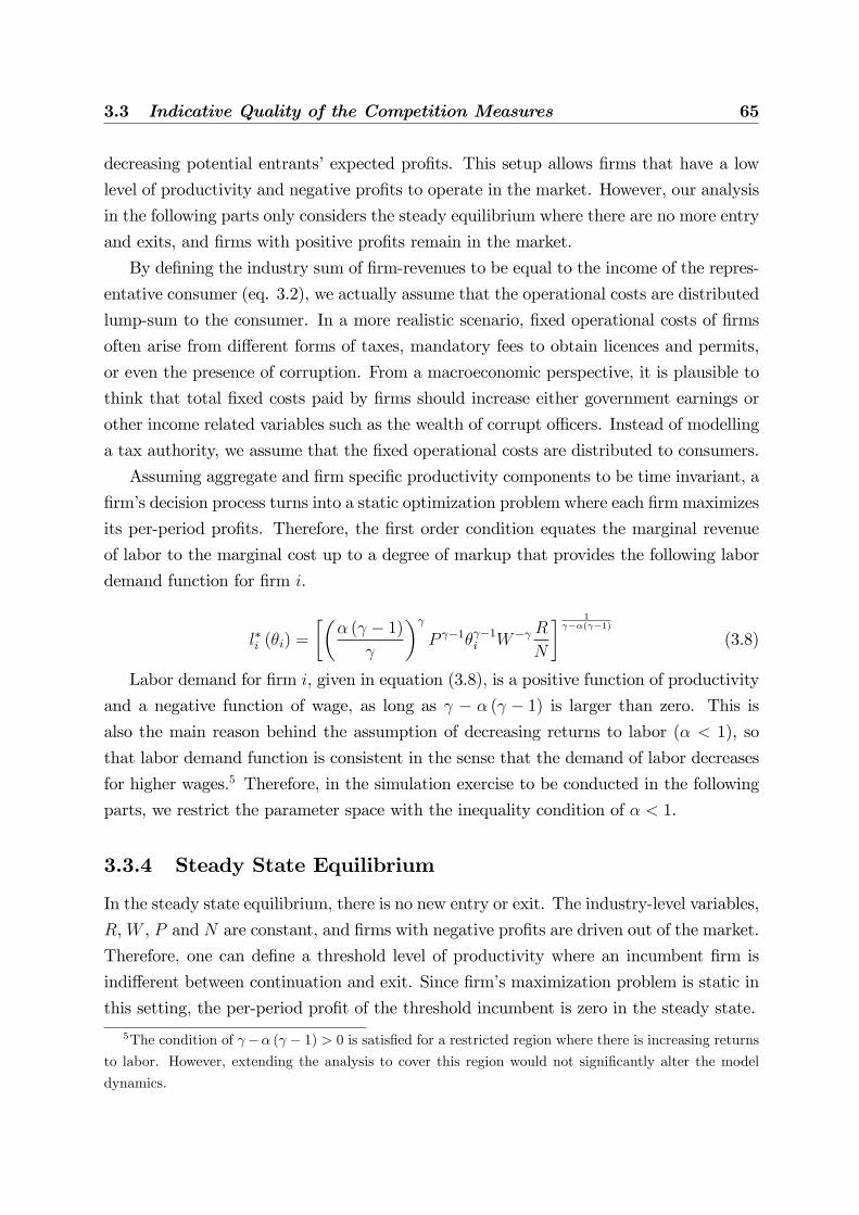
3.3 Indicative Quality of the Competition Measures 65
decreasing potential entrants�expected pro�ts. This setup allows �rms that have a low
level of productivity and negative pro�ts to operate in the market. However, our analysis
in the following parts only considers the steady equilibrium where there are no more entry
and exits, and �rms with positive pro�ts remain in the market.
By de�ning the industry sum of �rm-revenues to be equal to the income of the repres-
entative consumer (eq. 3.2), we actually assume that the operational costs are distributed
lump-sum to the consumer. In a more realistic scenario, �xed operational costs of �rms
often arise from di¤erent forms of taxes, mandatory fees to obtain licences and permits,
or even the presence of corruption. From a macroeconomic perspective, it is plausible to
think that total �xed costs paid by �rms should increase either government earnings or
other income related variables such as the wealth of corrupt o¢ cers. Instead of modelling
a tax authority, we assume that the �xed operational costs are distributed to consumers.
Assuming aggregate and �rm speci�c productivity components to be time invariant, a
�rm�s decision process turns into a static optimization problem where each �rm maximizes
its per-period pro�ts. Therefore, the �rst order condition equates the marginal revenue
of labor to the marginal cost up to a degree of markup that provides the following labor
demand function for �rm i.
l�i (�i) =
��� ( � 1)
� P �1� �1i W� R
N
� 1 ��( �1)
(3.8)
Labor demand for �rm i, given in equation (3.8), is a positive function of productivity
and a negative function of wage, as long as � � ( � 1) is larger than zero. This isalso the main reason behind the assumption of decreasing returns to labor (� < 1), so
that labor demand function is consistent in the sense that the demand of labor decreases
for higher wages.5 Therefore, in the simulation exercise to be conducted in the following
parts, we restrict the parameter space with the inequality condition of � < 1.
3.3.4 Steady State Equilibrium
In the steady state equilibrium, there is no new entry or exit. The industry-level variables,
R,W , P and N are constant, and �rms with negative pro�ts are driven out of the market.
Therefore, one can de�ne a threshold level of productivity where an incumbent �rm is
indi¤erent between continuation and exit. Since �rm�s maximization problem is static in
this setting, the per-period pro�t of the threshold incumbent is zero in the steady state.
5The condition of �� ( � 1) > 0 is satis�ed for a restricted region where there is increasing returnsto labor. However, extending the analysis to cover this region would not signi�cantly alter the model
dynamics.

66 Measuring Competition in a Frictional Economy
�T��T ;W �; P �; N�; R�
�= 0 (3.9)
�T is the threshold productivity level to stay in the market, and the starred variables
represent steady state equilibrium values. In case a �rm�s productivity is lower than this
threshold level, its expected pro�ts is negative, so that exit is the optimal decision.
Since a �rm cannot directly observe others�productivity draws, it develops its expect-
ations over the known distribution function. Thus, expected total sales can be calculated
by an integral over the revenues (ri) of incumbent �rms that could exceed the threshold
productivity level (�T ) of the industry.
E [R�] = N
1Z�T
ri (�i;W�; P �; N�; R�) f (�) d� (3.10)
In equation (3.10), R� appears on the both sides of the identity, where it stands for
the income level of the consumer on the right-hand side and the industry sum of revenues
on the left-hand side, which are equal in the equilibrium.
The expected aggregate price index is given by the following formula.
E [P �] =
241Z�T
pi (�i; P�; N�; R�)1� f (�) d�
351=(1� ) (3.11)
Therefore, expected industry-wide price index is calculated by an integral over incum-
bents�prices.
The equilibrium free entry condition requires the expected value of entry to be driven
to zero.6 Therefore, the free entry condition can be written as follows.
E�V E�=
1Z�1
�i (�i;W�; P �; N�; R�) f (�) d� = 0 (3.12)
According to equation (3.12) a potential entrant �rm calculates the value of entry by
considering any possible productivity draw within the interval (�1; 1).7
6In the model setup, �rms make the entry decision before they realize their productivity. Moreover,
after paying the �xed operational cost, �rms observe their productivity draw simultaneously with the
production process. Therefore, �rms are not allowed to exit the market just after the entry decision and
before paying the �xed cost. In other words, every entrant needs to pay the �xed cost and start producing
its variety in order to realize its productivity performance, so that exiting before producing would not be
optimal.7It is also possible to formulate the free entry condition in a more general way by equating the integral
over �rms�net (variable) pro�ts to �xed operational cost (�), because the �xed costs enter into pro�t
function linearly and the integral covers all possible productivity draws.

3.3 Indicative Quality of the Competition Measures 67
Lastly, in the equilibrium, total labor supply�1 = LS
�equates total labor demand,
so that steady state labor market clearing condition can be represented by the below
identity.
1 = N�1Z�T
li (�i;W�; P �; N�; R�) f (�) d� (3.13)
The right-hand side of equation (3.13) is the expected �rm-level labor demand times
the number of �rms that gives the expected total labor demand in the equilibrium.
As a result, the equilibrium in the model industry is characterized by �ve conditions,
and the �ve endogenous variables, P �, W �, N�, R� and �T , can be fully identi�ed in the
steady state.
3.3.5 The Measures of Competition
This section formulates three "empirical" measures of competition in accordance with
our theoretical setting. The main di¤erence between the empirical and theoretical formu-
lations of competition indices stems from the presence of �xed costs. Namely, while in
the standard theoretical formulations of price-cost margin and pro�t elasticity, only the
variable costs are considered, in the empirical analysis it is often di¢ cult to disentangle
variable and �xed costs. In particular, expenditures on labor input are mostly de�ned to
be variable, but in reality, an important portion of labor expenses are �xed (e.g. Oi, 1962).
Therefore, our total cost formulation also includes the �xed cost of operation (�), while
the results of the following simulation exercise are not really sensitive to the magnitude
of �xed costs.
The de�nitions given in this section will be used in the simulation exercise to analyze
the indicative performances of the competition measures by observing their reactions to
the changes in the elasticity of substitution for alternative parameter settings. For this
purpose, the substitution elasticity of demand ( > 1) is considered as the determinant of
the intensity of product market competition in the model industry. As rises, ( � 1) = approaches 1 indicating a perfect substitution among product varieties that constitutes the
highest level of interaction among �rms. To simplify the interpretations, all the measures
of competition are formulated in a way that a higher value corresponds to a higher degree
of competition.
Inverse Price-Cost Margin (iPCM)

68 Measuring Competition in a Frictional Economy
At the �rm level, the inverse price-cost margin (ipcm) is given by the ratio of total
costs to revenues.
ipcmi =Wli + �
ri(3.14)
In the above formulation, ipcm consist of two ratios that we name the variable (Wli=ri)
and �xed (�=ri) components. The variable component can be expressed in terms of price-
cost markup, namely, the total variable costs to revenues ratio is equivalent to factor share
to markup ratio in the steady state. Therefore, the following identity is valid for every
�rm in the model industry.Wliri
=�
�(3.15)
In equation (3.15), � = = ( � 1) represents the markup that is a negative function ofsubstitution elasticity, so that the variable cost component in �rm-level ipcm is increasing
in . However, as we will see in the simulation analysis, the �xed cost component may not
necessarily be an increasing function of . This is because, the total size of the industry
in terms of total revenues increases with due to the rise in the total number of �rms
and varieties. Therefore, when new entries are restricted by a �xed cost, incumbent �rms
may expand their market share. As a direct consequence of more intense interaction,
less e¢ cient �rms may exit the market that would further facilitate remaining �rms to
increase their sales in the equilibrium. Therefore, the reaction of ipcm to the changes
in the substitution elasticity depends on the relative importance of variable and �xed
components that may move in the opposite directions as competition intensi�es.
In the steady state, the industry-level iPCM can be calculated by the ratio of total
costs to revenues. This formulation is equivalent to the weighted average of �rm-level
ipcm and can be given by the following formula.
iPCM = 1� ��
R�(3.16)
In the above formulation, �� =R1�T�if (�) d� represents the expected total pro�ts in
the steady state. As the share of industry pro�ts (costs) in total sales decreases (increases),
iPCM approaches to 1, which may or may not be interpreted as a rise in the intensity of
competition depending on the steady state dynamics of the model industry.8
8In the steady state, the variable cost component of the industry-iPCM is equal toW �=R�. Therefore,
if we would rely on a partial equilibrium setting with exogenous wage, the reaction of the industry-level
iPCM to would be the same as the reaction of the �xed cost component. Namely, if more intense
interaction leads the market to expand in terms of revenues, the iPCM would be perfectly negatively
correlated with in the case of constant wage. However, the general equilibrium properties used in
the model takes into account the e¤ect of competition on wages, so that the direction of the relationship
between iPCM and is not straightforward and can be nonlinear depending on the steady state dynamics.

3.3 Indicative Quality of the Competition Measures 69
Theoretical Pro�t Elasticity (TPE)
The pro�t elasticity method (Boone, 2008b) suggests that the ratio of the pro�t of an
e¢ cient �rm to an ine¢ cient one is higher when competition is more intensive. Namely,
higher intensity of interaction leads the ine¢ cient �rms to su¤er more or bene�t less from
competition than the e¢ cient one.
The pro�t elasticity method can be simply expressed by assuming an industry with
two �rms, where �i represents the per-period pro�ts of �rm i. If �rm 2 is more e¢ cient
than �rm 1, holding everything else the same for these two �rms, one would expect the
pro�ts of the more e¢ cient �rm to be higher (�2 > �1). The method of pro�t elasticity
argues that if competition is more intensive at time t+1 than it is at time t, the inequality
(�2=�1)t+1 > (�2=�1)t holds. In other words, more intense competition widens the pro�t
gap between e¢ cient and ine¢ cient units, while some of the ine¢ cient ones may be driven
out of the market as a direct consequence of intensive interaction.
The mechanism behind the pro�t elasticity described above can be generalized for N
number of �rms. Assuming �rm j is the benchmark and the least e¢ cient production unit
in an industry, the condition �i > �j holds for all i 6= j. Therefore, if we draw a curve ona two dimensional �gure where �rms�relative e¢ ciency is on the horizontal and relative
pro�ts is on the vertical axis, the absolute value of the slope of the relative pro�ts curve
on a given point would be higher when competition is intensi�ed.
In the theoretical model (Boone, 2008a; 2008b), Boone makes use of exogenous �rm-
level marginal costs as the source of �rm-level heterogeneity and the measure of e¢ ciency.
In our model, �rm-level e¢ ciency is captured in the productivity parameter �i. Therefore,
a measure of pro�t elasticity can be derived by the following formula.
log
��i�j
�= �A+ � log
��i�j
�(3.17)
In the above equation, � represents the measure of the elasticity of relative pro�ts
to relative productivity, and �A is the �xed term that captures other exogenous factors
a¤ecting pro�tability. Throughout the rest of this chapter, we refer to the productivity
elasticity of pro�ts, �, as the "theoretical" pro�t elasticity (TPE).
In the following parts, our discussion will be mainly on �nding a suitable e¢ ciency
index to be used in the measurement of pro�t elasticity. However, one �rst needs to check
whether the abovementioned relationship holds for our model industry. Namely, we need
less e¢ cient �rms to have lower pro�ts than more e¢ cient ones in order to de�ne the
pro�t elasticity in our theoretical setting.
Proposition 1 Firm pro�ts are monotonically increasing in �.
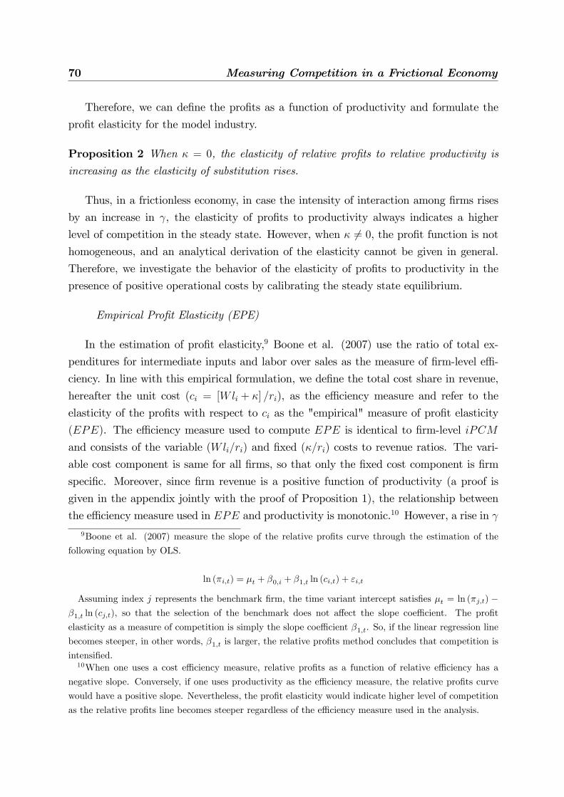
70 Measuring Competition in a Frictional Economy
Therefore, we can de�ne the pro�ts as a function of productivity and formulate the
pro�t elasticity for the model industry.
Proposition 2 When � = 0, the elasticity of relative pro�ts to relative productivity is
increasing as the elasticity of substitution rises.
Thus, in a frictionless economy, in case the intensity of interaction among �rms rises
by an increase in , the elasticity of pro�ts to productivity always indicates a higher
level of competition in the steady state. However, when � 6= 0, the pro�t function is nothomogeneous, and an analytical derivation of the elasticity cannot be given in general.
Therefore, we investigate the behavior of the elasticity of pro�ts to productivity in the
presence of positive operational costs by calibrating the steady state equilibrium.
Empirical Pro�t Elasticity (EPE)
In the estimation of pro�t elasticity,9 Boone et al. (2007) use the ratio of total ex-
penditures for intermediate inputs and labor over sales as the measure of �rm-level e¢ -
ciency. In line with this empirical formulation, we de�ne the total cost share in revenue,
hereafter the unit cost (ci = [Wli + �] =ri), as the e¢ ciency measure and refer to the
elasticity of the pro�ts with respect to ci as the "empirical" measure of pro�t elasticity
(EPE). The e¢ ciency measure used to compute EPE is identical to �rm-level iPCM
and consists of the variable (Wli=ri) and �xed (�=ri) costs to revenue ratios. The vari-
able cost component is same for all �rms, so that only the �xed cost component is �rm
speci�c. Moreover, since �rm revenue is a positive function of productivity (a proof is
given in the appendix jointly with the proof of Proposition 1), the relationship between
the e¢ ciency measure used in EPE and productivity is monotonic.10 However, a rise in
9Boone et al. (2007) measure the slope of the relative pro�ts curve through the estimation of the
following equation by OLS.
ln (�i;t) = �t + �0;i + �1;t ln (ci;t) + "i;t
Assuming index j represents the benchmark �rm, the time variant intercept satis�es �t = ln (�j;t) ��1;t ln (cj;t), so that the selection of the benchmark does not a¤ect the slope coe¢ cient. The pro�t
elasticity as a measure of competition is simply the slope coe¢ cient �1;t. So, if the linear regression line
becomes steeper, in other words, �1;t is larger, the relative pro�ts method concludes that competition is
intensi�ed.10When one uses a cost e¢ ciency measure, relative pro�ts as a function of relative e¢ ciency has a
negative slope. Conversely, if one uses productivity as the e¢ ciency measure, the relative pro�ts curve
would have a positive slope. Nevertheless, the pro�t elasticity would indicate higher level of competition
as the relative pro�ts line becomes steeper regardless of the e¢ ciency measure used in the analysis.

3.3 Indicative Quality of the Competition Measures 71
directly e¤ects the e¢ ciency measure of EPE in the steady state equilibrium. The main
di¤erence between TPE and EPE, thus, arises in the measure of �rm-level e¢ ciency, as
we will see below.
If �rm revenue is a positive function of , a rise in leads the e¢ ciency measures
(unit costs) of any two �rms to converge due to a decrease in the �rm-speci�c, �xed cost
component, and an increase in the �rm-invariant, variable cost component. This would
further lead the cost e¢ ciency ratio of more to less e¢ cient �rm (ci=cj where cj > ci) to
rise with in the steady state. Moreover, if the rate of the increase in ci=cj is higher
than the increase in �i=�j, EPE would indicate a fall in competition as the elasticity of
substitution rises.
In the simulation of the theoretical model, we need two points on the relative pro�ts
curve to retrieve the slope of the linear approximation. This means evaluating three
�rms with three di¤erent e¢ ciency levels where the least e¢ cient �rm is taken to be the
benchmark �rm. It is important to keep these �rms, (and their productivity levels) �xed
throughout di¤erent parameter settings. One reason for this is possible non-linearity of
the relative pro�ts curve, which would change the slope for alternative �rm sets, even if
the relationship between pro�ts and productivity stays same. Moreover, its also crucial
that these three �rms should stay in the market during di¤erent experiments, so that we
require their productivity values to be higher than any possible productivity threshold
that may occur in alternative cases. Assuming the e¢ ciency ordering of the three �rms is
�3 > �2 > �1, so that c3 < c2 < c1, the theoretical pro�t elasticity is calculated as follows.
TPE =
�3 (�3)
�1 (�1)� �2 (�2)�1 (�1)
�3�1� �2�1
(3.18)
Similarly, in order to calculate EPE, one can substitute �i�s with ci�s in the above
formula and multiply the right hand side with �1.
3.3.6 Iterative Solution of the Steady State
The �rst step in the simulation analysis is to calculate the steady state values of the
industry-wide endogenous variables that are R;W;P;N and �T . In order to do that, we
apply an iterative method over the equilibrium identities listed in the previous part under
the title of "steady state equilibrium". Given the exogenous parameter values for ; �; �; �
and �, the procedure starts by assuming initial values for W (0), P (0) and �T (0).
In the benchmark equations of the model, the income level shows up in the form of
average �rm sales (~r = R=N), so that we use ~r in the formulation of the simulation al-

72 Measuring Competition in a Frictional Economy
gorithm. Given the initial values of wage, aggregate price level and threshold productivity,
one can calculate the steady state value of ~r through equation (3.10). Although the right-
hand side of the equation is also a function of ~r, the average income level is independent
of idiosyncratic productivity (�) at the steady state. Thus, one can take ~r out of the
integral. Given W (0), P (0) and �T (0), equation (3.10) provides an explicit identity for the
average income level (~r). The identity for the expected average revenue can be given as
follows.
E [~r] =
0@1Z�T
���
�W
��P�i
� 1���
f (�) d�
1A���1��
(3.19)
In the next step, for given ~r(1), W (0) and P (0), one can update the initial guess of the
threshold level of productivity through threshold incumbent�s equilibrium condition given
in equation (3.9). Using the new value for the threshold productivity (�T (1)) and for given
W (0), ~r(1) and P (0), the initial guess of the aggregate price index is updated through the
steady state aggregate price identity (eq. 3.11). In the next step, the initial guess of the
aggregate wage level is updated by labor market clearing condition (eq. 3.13). Lastly,
the number of �rms or varieties are calculated through the free entry condition given in
equation (3.12) by using the updated values of the endogenous variables (~r(1), W (1), P (1)
and �T (1)) .
After updating the initial guesses for the �ve endogenous variables, we repeat the pro-
cedure with the new values, and the iterative algorithm is continued until the convergence
is achieved in the �ve equilibrium conditions simultaneously.
3.3.7 Calibration of Parameters
We have a set of 5 exogenous parameters, namely the elasticity of substitution ( ), the
standard deviation (�) and the mean (�) of the productivity distribution, the labor elasti-
city of production (�) and the �xed operational cost (�), for which we need to assume
numeric values in the simulation analysis. Rather than assigning a single value, we con-
sider an interval for each parameter and conduct robustness checks simultaneously with
the interpretations of the results.
We consider the e¤ects of alternative degrees of returns from labor input by allowing �
to be equal to 0:7 and 0:9 respectively. In the econometric part, the calculated coe¢ cient
of variation for the productivity distribution in the manufacturing industries of Ukraine
ranges between 1 and 50. The coe¢ cient of variation corresponds to the ratio of the
standard deviation to mean, �=�, so that � 2 f5; 15g and � 2 f0:5; 1:5g are set to

3.3 Indicative Quality of the Competition Measures 73
match approximately with the observed productivity dispersion in the data. The elasticity
of substitution, , is considered to lie between 1:3 and 2:8, so that we ignore very high
degrees of substitutability where price-cost mark-up is close to 1, and the model dynamics
tend to replicate the predictions of standard perfect competition model. Lastly, the value
of the operational cost (�) is allowed to range between 4 and 6, so that � is approximately
equal to 10% of the revenue of average �rm in the industry.
3.3.8 Simulation Results
This section presents the results of the simulation analysis. The results are interpreted
by evaluating the performances of the empirical competition indices according to their
responses to changes in the elasticity of substitution for alternative parameter settings.
The following paragraphs elaborate alternative sets of simulations each considering two
alternative values for a given exogenous parameter. In all the �gures displayed under
the title of simulation results, the elasticity of substitution lies on the horizontal and the
respective endogenous variables are on the vertical axis.
In the �rst set of simulations, the steady state equilibrium values of the respective
endogenous variables are plotted against the elasticity of substitution ( 2 [1:3; 2:8]) foralternative returns to labor input (� 2 f0:7; 0:9g). The two variables that determine thedegree of productivity dispersion are set to � = 10 and � = 1, and the value of the
operational cost is � = 5.

74 Measuring Competition in a Frictional Economy
Figure 3.1: Simulation Results*
1.4 1.6 1.8 2 2.2 2.4 2.6 2.8 31.5
2
2.5
3
3.5
4
4.5
5
γ
Rev
enue
"Revenue" by "α"
α=0.7
α=0.9
1.4 1.6 1.8 2 2.2 2.4 2.6 2.8 30.2
0.4
0.6
0.8
1
γ
Pro
fits
"Profits" by "α"
α=0.7
α=0.9
1.4 1.6 1.8 2 2.2 2.4 2.6 2.8 30
2.5
5
7.5
10x 10
4
γ
Firm
Siz
e
"Firm Size" by "α"
α=0.7α=0.9
1.4 1.6 1.8 2 2.2 2.4 2.6 2.8 30
0.2
0.4
0.6
0.8
1
1.2x 10
3
γ
#firm
s
"#firms" by "α"
α=0.7
α=0.9
*The other parameters of the model are set to �=10, �=1 and �=5.
The top panel of Figure 3.1 displays the reaction of �rm-level revenue and pro�ts to
the changes in the elasticity of substitution for alternative degrees of returns to labor.
As the intensity of interaction increases, both expected pro�ts and revenues rise in the
steady state. According to the bottom right panel, the number of �rms goes up with ,
which implies that aggregate income expands with higher levels of competition.
If the total rise in revenues outpaces the increase in pro�ts, industry-wide iPCM falls.
The reaction of EPE depends on the relative importance of the increase in the shrinking
�xed-cost component (�=r) of the relative e¢ ciency measure (ci=cj).
The lower left panel of Figure 3.1 shows that �rm size measured by the amount of
labor used in production is a decreasing function of the elasticity of substitution. Since,
enters into the production function through labor input, the expected quantity of �rm
output falls with for given �. Therefore, we can conclude that the positive e¤ect of
on expected �rm revenues is mainly driven by the rise in �rm-level prices, which will be
further explored in the following sets of simulations.
The degree of returns to labor (�) also a¤ects the steady state equilibrium values of
the endogenous variables. The expected �rm size is lower for higher values of �, and total

3.3 Indicative Quality of the Competition Measures 75
revenues and pro�ts are positively correlated with the degree of returns to labor in the
equilibrium. However, the main picture of the industry is not really sensitive to changes
in � as we will further see below.
Figure 3.2: Simulation Results*
1.4 1.6 1.8 2 2.2 2.4 2.6 2.8 34.5
5
5.5
6
6.5
7
7.5
γ
EP
E
"EPE" by "α"
α=0.7
α=0.9
1.4 1.6 1.8 2 2.2 2.4 2.6 2.8 30.74
0.78
0.82
0.86
0.9
γ
iPC
M
"iPCM" by "α"
α=0.7
α=0.9
1.4 1.6 1.8 2 2.2 2.4 2.6 2.8 31
1.5
2
2.5
3
γ
TPE
"TPE" by "α"
α=0.7
α=0.9
1.4 1.6 1.8 2 2.2 2.4 2.6 2.8 36.5
7
7.5
8
8.5
9
9.5
γ
θT
"θT" by "α"
α=0.7
α=0.9
*The other parameters of the model are set to �=10, �=1 and �=5.
Figure 3.2 shows the responses of the three competition indicators and the threshold
level of productivity to changes in the degree of substitutability. The upper left panel of
the �gure displays that EPE is negatively correlated with the elasticity of substitution,
when substitution elasticity is low. However, the relationship turns out to be positive
as rises. Therefore, the increase in the relative e¢ ciency measure of EPE outpaces
the rise in the relative pro�ts for lower values of . As the elasticity of substitution
further increases, the rise in the �rm invariant variable-cost component (�=�) becomes
dominant over the decrease in the �xed-cost component (�=r). Thus, the rate of the rise
in the relative e¢ ciency measure (ci=cj where ci = �=� + �=ri) slows down as competition
intensi�es. For su¢ ciently high values of , EPE is positively correlated with the true
intensity of interaction among �rms.
In addition, higher � lowers the value of at the point where EPE reaches a minimum.
This is because the relative importance of the variable-cost component in the �rm-level

76 Measuring Competition in a Frictional Economy
e¢ ciency index rises, while the �xed-cost component shrinks with higher returns from
labor.
As a result, the relative e¢ ciency measure reacts to the changes in and, EPE does
not re�ect the true intensity of competition when the elasticity of substitution is relatively
low.
In the upper right panel of Figure 3.2, iPCM exhibits a negative correlation with the
level of competition, where the negative relationship weakens as rises.11 The downward
sloping iPCM curve is mainly driven by the negative relation between the �xed-cost
component and substitution elasticity that weakens as further increases.
Intuitively, the negative relationship between iPCM and heavily relies on the pres-
ence of operational costs. As shown in Figure 3.1, the overall income level increases with
higher degrees of competition, but whether incumbents would increase their pro�t to sale
ratios as a response to depends on the entry and exit dynamics. Therefore, if we di-
minish the expected value of entry and facilitate the exit of less e¢ cient incumbents by
introducing a positive operational cost, the incumbent �rms that are productive enough
to stay in the market would enhance their pro�tability as the level of competition rises.
In other words, more intense interaction provides high productivity incumbents with the
opportunity to push low productivity �rms out of the market, while the competitive pres-
sure from new entries is restricted by the cost parameter. This can be also seen at the
lower right panel of Figure 3.2, where the threshold productivity to stay in the market,
�T , goes up with higher values of .
Conversely, one can think of the income expanding role of more intense competition
to have an opposite e¤ect that encourage potential �rms to enter into the market. There-
fore, for su¢ ciently high values of , the negative correlation between iPCM and the
substitution elasticity weakens.
As the degree of returns from labor increases, iPCM rises for given . The negative
correlation between iPCM and further weakens with higher �. This is mainly due
to the increasing importance of labor input in comparison to idiosyncratic productivity
parameter in the production function, so that the productivity advantage of more e¢ cient
units disappears as labor becomes the dominant component in the production function.
11The results for values of higher than 2:8 are not reported, basically because product variation
disappears, and the model industry tends to replicate the dynamics of the perfectly competitive market
for higher degrees of substitutability. However, all the measures of competition listed in this paper are
theoretically positively correlated with the real intensity of interaction as the model approaches to perfect
competition.

3.3 Indicative Quality of the Competition Measures 77
The lower left panel of Figure 3.2 shows that TPE is monotonically increasing in ,
and the relationship is almost linear for alternative values of �.
Figure 3.3: Simulation Results*
1.4 1.6 1.8 2 2.2 2.4 2.6 2.8 31.2
1.4
1.6
1.8
2
2.2
2.4
2.6x 10
3
γ
Pric
e in
d.
"Price ind." by "α"
α=0.7
α=0.9
1.4 1.6 1.8 2 2.2 2.4 2.6 2.8 30
0.5
1
1.5
2
2.5
3x 10
3
γW
age
"Wage" by "α"
α=0.7
α=0.9
1.4 1.6 1.8 2 2.2 2.4 2.6 2.8 30
0.5
1
1.5
2x 10
4
γ
Pric
e
"Price" by "α"
α=0.7
α=0.9
1.4 1.6 1.8 2 2.2 2.4 2.6 2.8 30
2
4
6
8
10x 10
4
γ
Out
put
"Output" by "α"
α=0.7α=0.9
*The other parameters of the model are set to �=10, �=1 and �=5.
According to the top panels of Figure 3.3, the industry-wide price index and the wage
level are boosted by more intense competition. This is a direct consequence of the income
expanding e¤ect of the elasticity of substitution, which raises aggregate nominal variables
in the steady state. Higher returns to labor, �, increases labor demand and wages, and
shifts the expected output curve up for given amount of labor, which in turn diminishes
the aggregate price index in the equilibrium for given .
The lower panel of Figure 3.3 shows that the �rm-level price and the quantity of output
move in the opposite directions as competition intensi�es. These asymmetric e¤ects of
competition on prices and quantities play a key role in the mechanism that cause iPCM
and EPE to deviate from the direction of the true intensity of interaction.
Since the quantity of output is a decreasing function of , the rise in the �rm revenues
with higher level of competition is mainly driven by the upward shift in the �rm-level
prices, so that the �xed and variable components involved in the �rm-level iPCM (as
well as in the e¢ ciency measure of EPE) move in the opposite directions. Therefore,

78 Measuring Competition in a Frictional Economy
if the empirical researcher would observe prices at the �rm-level, it would be possible
to extract the distorting part of EPE; for instance, a quantity based input to output
ratio would be a suitable e¢ ciency measure that would lead EPE to be monotonically
increasing in .
In our theoretical setting, it is also possible to analytically show the existence of
distorting price e¤ects in the e¢ ciency measures based on nominal variables. It follows
directly from the production function that the quantity of output is a positive function of
productivity. Conversely, the variety speci�c price function, which can be derived from the
demand identity given in equation (3.5), is a negative function of productivity. Therefore,
if one uses revenues in the place of the quantity of output with the aim of, for instance,
calculating a cost e¢ ciency index as in the original pro�t elasticity method (Boone et
al., 2007) or a labor productivity index, the empirical e¢ ciency measure would involve
price e¤ects that may be negatively correlated with the quantities. If this is the case,
the index would be a distorted measure of actual e¢ ciency or productivity. Moreover,
de�ating revenues with an aggregate price index would be also problematic due to the
negative correlation between the �rm-level prices and productivity, so that the empirical
productivity index based on price-adjusted revenues would underestimate (overestimate)
the actual productivity level of more (less) e¢ cient production units.12
An important result of the simulation exercise is that empirical analysis requires a
robust measure of e¢ ciency that takes into account price variation in the calculation of
pro�t elasticity. Otherwise, the e¢ ciency measure of pro�t elasticity would be sensitive
to the degree of imperfect competition and the results would be signi�cantly biased.
In the second set of simulations, we investigate the e¤ects of the substitution elasticity
on the industry dynamics for alternative degrees of productivity dispersion. While doing
so, the constant industry-wide component of productivity is � = 1, and the standard
deviation of productivity distribution (�) takes two alternative values. As in the �rst set
of simulations, the operational cost is set to � = 5; and the returns from labor is � = 0:9.
As the degree of �rm heterogeneity diminishes, the industry collapses into a model of a
single representative �rm with homogeneous output, where the e¤ects of the substitution
elasticity vanishes. Conversely, as the standard deviation of productivity distribution
increases, the e¤ects of competition on industry dynamics are ampli�ed. We do not
report the behavior of �rm size, revenues, pro�ts and output in response to �. Except for
the expected �rm size, these variables increase with � for a given degree of substitutability
12For further discussion and empirical support on the negative relationship between �rm-level prices
and the quantity based productivity see Foster et al. (2008).
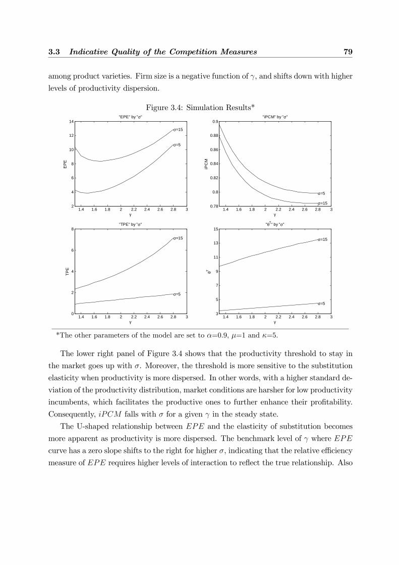
3.3 Indicative Quality of the Competition Measures 79
among product varieties. Firm size is a negative function of , and shifts down with higher
levels of productivity dispersion.
Figure 3.4: Simulation Results*
1.4 1.6 1.8 2 2.2 2.4 2.6 2.8 32
4
6
8
10
12
14
γ
EP
E
"EPE" by "σ"
σ=5
σ=15
1.4 1.6 1.8 2 2.2 2.4 2.6 2.8 30.78
0.8
0.82
0.84
0.86
0.88
0.9
γ
iPC
M
"iPCM" by "σ"
σ=5
σ=15
1.4 1.6 1.8 2 2.2 2.4 2.6 2.8 30
2
4
6
8
γ
TPE
"TPE" by "σ"
σ=5
σ=15
1.4 1.6 1.8 2 2.2 2.4 2.6 2.8 33
5
7
9
11
13
15
γ
θT
"θT" by "σ"
σ=5
σ=15
*The other parameters of the model are set to �=0.9, �=1 and �=5.
The lower right panel of Figure 3.4 shows that the productivity threshold to stay in
the market goes up with �. Moreover, the threshold is more sensitive to the substitution
elasticity when productivity is more dispersed. In other words, with a higher standard de-
viation of the productivity distribution, market conditions are harsher for low productivity
incumbents, which facilitates the productive ones to further enhance their pro�tability.
Consequently, iPCM falls with � for a given in the steady state.
The U-shaped relationship between EPE and the elasticity of substitution becomes
more apparent as productivity is more dispersed. The benchmark level of where EPE
curve has a zero slope shifts to the right for higher �, indicating that the relative e¢ ciency
measure of EPE requires higher levels of interaction to re�ect the true relationship. Also

80 Measuring Competition in a Frictional Economy
in this set of simulations, TPE is monotonically increasing in for alternative degrees of
�rm heterogeneity, and the sensitivity of TPE to rises with �.13
When the �xed cost is zero (� = 0), iPCM is identical to factor elasticity to mark-
up ratio (�=�) which monotonically increases with the elasticity of substitution. The
positive correlation between iPCM and is broken with the introduction of �xed costs
into the model industry. The e¢ ciency measure used in EPE also is identical to �=�,
and thus is the same for all �rms, so that EPE is not measurable in the case of � = 0.
In addition, the TPE is monotonically increasing in when operational cost is zero as
stated in Proposition 2 and proved in the appendix. However, as long as operational cost
is strictly positive, the responses of the respective competition indices to the changes in
the elasticity of substitution are irrespective of the alternative values of �.
In the third set of simulations, the relationship between the level of competition and
the endogenous variables are investigated for alternative values of the operational cost
parameter, namely, � 2 f4; 6g. The other parameters are set in accordance with previousdiscussions, so that � = 0:9, � = 10 and � = 1.
Figure 3.5: Simulation Results*
1.4 1.6 1.8 2 2.2 2.4 2.6 2.8 30
0.4
0.8
1.2
1.6x 10
3
γ
#firm
s
"#firms" by "κ"
κ=4
κ=6
1.4 1.6 1.8 2 2.2 2.4 2.6 2.8 30
0.5
1
1.5
2x 10
4
γ
Firm
Siz
e
"Firm Size" by "κ"
κ=4κ=6
*The other parameters of the model are set to �=0.9, �=1 and �=10.
When the �xed cost of operation is higher, the total size of the industry (R) shrinks
and concentration rises in the steady state. Figure 3.5 shows that the total number of �rms
falls, and the expected �rm size in terms of the amount of labor employed in production
expands with �. In that case, the negative relationship between �rm size and , and
the positive correlation of the number of �rms with the elasticity of substitution are still
valid for alternative values of the cost parameter. However, higher � facilitates the exit
13As in the empirical part, we interpret the coe¢ cient of variation (�=�) as an indicator of the dispersion
in the productivity distribution. Therefore, a fall in � creates the same impact as an increase in �. Hence,
we do not display the e¤ects of � on the industry dynamics separately.

3.3 Indicative Quality of the Competition Measures 81
process of less e¢ cient �rms and lowers the expected value of entry, so that remaining
�rms increase their market share in the steady state. Thus, the market concentration rise
without any change in the degree of the substitutability among the product varieties.
Figure 3.6: Simulation Results*
1.4 1.6 1.8 2 2.2 2.4 2.6 2.8 30
0.2
0.4
0.6
0.8
1
1.2
1.4
γ
Pro
fits
"Profits" by "κ"
κ=4
κ=6
1.4 1.6 1.8 2 2.2 2.4 2.6 2.8 31
2
3
4
5
6
γ
Rev
enue
"Revenue" by "κ"
κ=4
κ=6
1.4 1.6 1.8 2 2.2 2.4 2.6 2.8 30
0.5
1
1.5
2
2.5
3x 10
3
γ
Wag
e
"Wage" by "κ"
κ=4
κ=6
1.4 1.6 1.8 2 2.2 2.4 2.6 2.8 31
1.2
1.4
1.6
1.8
2
2.2
x 103
γ
Pric
e in
d.
"Price ind." by "κ"
κ=4
κ=6
*The other parameters of the model are set to �=0.9, �=1 and �=10.
As shown in the lower panel of Figure 3.6, the expected wage level and the industry-
wide price index decrease in equilibrium for higher �. This is mainly due to the fall in the
total income created in the industry, because monetary resources are further transferred
from the production process to the representative consumer as a component of income.
The top panel of Figure 3.6 shows that expected revenues and pro�ts increase with �.
The upward shift in �rm revenues is proportional to the rise in �, so that the share of the
�xed operational cost in a �rm�s revenue stays same for alternative values of operational
cost. Variable cost to revenue ratio is also independent of �, so that iPCM does not
change with the magnitude of frictions in the industry as long as � > 0. Since operational
costs are the same for all �rms, every incumbent �rm experiences a proportional change
in pro�ts as a response to �. Therefore, the EPE and TPE are independent of the
alternative positive values of � in the steady state. However, for given , concentration

82 Measuring Competition in a Frictional Economy
based measures of competition would indicate lower intensity of interaction with higher
�xed costs of operation.
3.4 Empirical Analysis of the Competition Indices
Throughout the theoretical discussions in the previous parts, we point out possible factors
that distort the measurement of product market competition by the inverse price-cost
margin (iPCM) and the empirical pro�t elasticity (EPE) methods.
iPCM deviates from the true direction of competition when we introduce the opera-
tional costs at the �rm-level. In that case, the �xed cost to revenue ratio falls with more
intense competition, which leads iPCM to be negatively correlated with the elasticity of
substitution for relatively lower degrees of substitutability among product varieties. Intu-
itively, the presence of operational costs lowers the expected value of entry and makes the
survival of ine¢ cient production units more di¢ cult, so that more e¢ cient incumbents
expand their market share and enhance their pro�tability as product market competition
intensi�es.
Firm-level iPCM also is used as the cost e¢ ciency measure of EPE, and does not
re�ect the true relative e¢ ciency between any two �rms when the elasticity of substitution
is relatively low. While competition leads the pro�t of more e¢ cient �rm to increase at a
higher rate than that of less e¢ cient one, the cost e¢ ciency levels (measured by total input
expenditures to revenue ratio) of the two �rms converge for more intense competition.
Thus, the relative e¢ ciency measure of EPE also rises with the elasticity of substitution
in the equilibrium. Given that the variable costs to revenue ratio is equal to �=� and
the same for all �rms, the convergence of the cost e¢ ciency measures of EPE is driven
by the shrinking �xed-cost component due to the rise in �rm revenues as a response to a
higher level of competition. As the elasticity of substitution increases starting from a low
value, the rate of increase in the relative cost e¢ ciency outpaces the rise in the relative
pro�ts. Therefore, EPE exhibits negative correlation with the substitution elasticity for
lower degrees of substitutability.
The reason behind the non-monotonic relationship between the elasticity of substi-
tution and EPE is that, the �rm-level e¢ ciency indicator used in EPE is sensitive to
the degree of imperfect competition. The e¢ ciency measure in EPE involves �rm-level
prices that move in the opposite direction with quantities as a response to more intense
�rm-to-�rm interaction, so that the �xed-cost to revenue ratio falls. If it would be possible
to observe quantities and prices separately or adjust the e¢ ciency measure to the degree
of imperfect competition, the bias in the calculation of EPE would be corrected.
3.4 Empirical Analysis of the Competition Indices 83
In most applied research with micro data, prices or quantities are unobserved at the
�rm-level. Researchers often use nominal data based e¢ ciency measures that are at best
de�ated with aggregate-level price indices. By doing so, one implicitly assumes that prices
are the same for all �rms in an industry that would be unrealistic, especially if there is
an important degree of imperfect competition and prices vary signi�cantly.
It would be possible to construct an alternative theoretical model by de�ning an exo-
genous �rm-level marginal cost parameter that serves as the source of �rm-level heterogen-
eity (e.g. Boone, 2008b). In this case, a pro�t elasticity measure that uses the exogenous
marginal costs as the e¢ ciency measure would be a theoretically robust indicator of com-
petition. However in reality, marginal costs are not directly observable at the �rm-level
either. Moreover, our concern in this study is to test the performance of a particular
type of pro�t elasticity that is commonly used in the empirical literature, namely the
pro�t elasticity that involves the expenditures to revenues ratio as the e¢ ciency measure.
Therefore, the point we emphasized in the theoretical part is that, regardless of the type
of the e¢ ciency measure, if it involves prices, the e¢ ciency measure would be sensitive
to the degree of imperfect competition, and the measure of pro�t elasticity would not be
perfectly correlated with the true level of competition. However, the pro�t elasticity based
on a robust measure of e¢ ciency, which is the exogenous productivity in the theoretical
model, is a robust measure of competition.
The next section sets out to �nd an empirically robust e¢ ciency measure that is not
sensitive to the degree of imperfect competition. Following that, comparisons will be
made between alternative competition measures. Finally, the empirical part concludes
with an analysis of the relationship between competition and productivity by considering
alternative productivity and competition indices.
3.4.1 Econometric Model
This part of the analysis aims to �nd a robust productivity measure that is not sensitive
to the degree of imperfect competition, so that we can robustly measure the intensity of
competition through the method of pro�t elasticity. The econometric algorithm described
in this section will be applied to a set of manufacturing �rms in Ukraine.
We assume that �rms produce according to a Cobb-Douglas production function,
whereQit, �it, Kit, Lit andMit are the �rm-level output, total factor productivity, capital,
labor and intermediate inputs respectively, and �i�s are the respective factor elasticity
parameters.
Qit = �itK�K
it L�L
it M�M
it (3.20)
84 Measuring Competition in a Frictional Economy
As we do not observe the actual quantity of output, we use de�ated revenues in
the estimation of productivity. In order to express the production function in terms of
revenues, we utilize the demand side of the theoretical model depicted in the previous
part. The �rm-level demand function (eq. 3.5) provides the following identity that links
the quantity of output to revenues of a �rm in equilibrium. By using this identity, we can
eliminate �rm-level prices from the formulation of the production process.
RitPt=
� �RtPt
� 1
Q1�
it (3.21)
As in the previous part, � = = ( � 1) represents the mark-up, and �Rt = N�1t
PNi Rit
is the average revenues in the model industry. Therefore, the aggregate term �Rt=Pt stands
for the industry-level demand shifter that provides a direct estimate of the industry speci�c
substitution elasticity.14 By combining equation (3.21) with the production function, one
can retrieve the following estimation equation at the industry-level where the lower case
letters represent the respective variables in logarithms. We further remove the aggregate
price index from the formulation, so that rit and �rt represent the logs of the revenues at
the �rm- and industry-level respectively that are de�ated by an aggregate price index.
rit = �0 + �E�rt + �Mmit + �Llit + �Kkit + �it=� + �it (3.22)
In the above formulation, �rt represents the amount that consumers are willing to spend
for a product variety. The coe¢ cient on �rt is equal to the inverse of the elasticity of sub-
stitution, namely �E = 1= . The coe¢ cients of the production factors satisfy the identity
�j = �j=� where j 2 fM; L; Kg. The markup parameter (�) that appears jointly with
the idiosyncratic productivity variable is fully identi�ed through the estimated coe¢ cient
of �E. For notational simplicity, � that shows up jointly with the productivity term in
equation (3.22) (�it=�) is omitted from the rest of the formulation of the econometric
model.
3.4.2 Estimation Methodology
The main di¢ culty in the estimation of production functions is the correlation between
the unobserved productivity shocks and the amount of inputs used in production. In
other words, a manager can observe her �rm�s productivity and use this knowledge in the
decision phase of the optimal amount of inputs. Therefore, one would expect a degree of
endogeneity in �rms�input usage to unobserved productivity.
14For discussions and examples of alternative demand speci�cations used in the production function
estimations see Levinsohn and Melitz (2004), Martin (2005), De Loecker (2007).

3.4 Empirical Analysis of the Competition Indices 85
In dealing with the endogeneity problem, our method derives from the estimation pro-
cedure with a proxy variable based on Olley and Pakes (1996) (OP). The OP deals with
the endogeneity of inputs by assuming that �rms immediately alter their investments in
response to productivity shocks. However, while using investments as a proxy for pro-
ductivity can solve the endogeneity problem, in practice, it creates its own shortcomings.
For example, investments may be too slow to react changes in productivity, and �rms
may not invest for some periods. So far the most common ways of dealing with the zero
investment problem is replacing them with a small positive number or deleting the o¤end-
ing observation. However, the former way may introduce additional error, and the latter
may cause severe selection bias. Especially in developing countries, �rms often decide not
to invest for reasons such as high levels of uncertainty, frictions in local �nancial markets
and high regulatory burden of investing. As supporting evidence, approximately one third
of the total number of the �rms report zero investment in our sample, which makes the
OP method impractical in our case.
In the estimation of the modi�ed production function, we utilize Levinsohn and Pet-
rin�s (2003) approach (LP) that suggests intermediate inputs to be used as a proxy for
the unobserved productivity. Besides solving the zero investment problem, the LP o¤ers
a better proxy for unobserved component in the sense that intermediate inputs can be
quickly adjusted to changing conditions.
We de�ne �rm�s intermediate inputs as a function of productivity where capital stock
is the state variable (mit (�it; kit)). Assuming mit is monotone in �it, we can invert the
equation of intermediate inputs to obtain the function to proxy the unobserved compon-
ent, namely �it = �it (mit; kit) where � (:) = m�1 (:). However, introducing this identity
into production function leads capital and intermediate inputs to appear multiple times
in the resulting equation. Therefore, the LP requires the factor elasticity coe¢ cients of
capital and intermediate inputs to be identi�ed in the second stage.
The LP routine combines all the terms that include intermediate inputs and capital
in a control function git(mit; kit) which is represented by a third order polynomial in
its arguments. The demand shifter (�rt) stands for average amount that consumers are
willing to spend on a variety. Therefore, the demand shifter is assumed to be independent
of today�s productivity shock, and the �rst stage regression equation takes the following
form.
rit = �E�rt + �Llit + git(mit; kit) + �it (3.23)
In the above regression equation, git(mit; kit) = �0 + �Mmit + �Kkit + �it (mit; kit)
constitutes the non-parametric part of the �rst stage estimation equation that takes into

86 Measuring Competition in a Frictional Economy
account the endogeneity between productivity and the amount of capital and intermediate
inputs used in the production.15
The second stage relies on the assumption that �it evolves as a �rst-order Markov
process. Namely, �it = E f�it j �it�1g + �it where �it is i.i.d. Thus, for any candidatevalues of ��K and �
�M ; the method retrieves the estimates of �it = git � ��Mmit � ��Kkit,
and a consistent nonparametric approximation of E f�it j �it�1g for given ��K and ��M can
be obtained from the �tted values of the following regression.
�it = �0 + �1�it�1 + �2�2
it�1 + �3�3
it�1 + �it (3.24)
We obtain the estimates of �K and �M by implementing GMM minimization method
as in the Levinsohn et al. (2004) on the joint error term given by the following equation16.
�it + �it = rit � �E�rt � ��Mmit � �Llit � ��Kkit � E \f�it j �it�1g (3.25)
The last term on the right-hand side of equation (3.25) stands for the productivity
expectations of the manager that is conditional on the previous period�s realization. In
order to identify �K and �M , we assume that the previous period�s levels of intermediate
inputs, labor and aggregate demand shifter are uncorrelated with this period�s productiv-
ity shock, so that the instrument matrix consists of mt�1, kt�1, lt�1 and �rt�1 provides
the moment conditions. Moreover, assuming today�s capital stock to be determined by
previous periods� investments that are uncorrelated with period t�s error, kt is further
used as an instrument for the GMM algorithm.
3.4.3 The Dataset
Our dataset consists of an annual sample of manufacturing �rms operated in Ukraine
during 2004-2007. Firms�revenues are represented by nominal sales after tax, and labor
input is total hours worked by full and part time employees of a �rm in a given year.
Intermediate inputs are proxied by the material expenses including the total nominal
costs of goods and services, acquired for the re-sale and realized without an additional
processing plus expenses for power. For capital, we use the reported depreciation of the
capital stock at a given enterprise.15As it is stated in Ackerberg et al. (2006), there is a possible correlation between labor input and
productivity which may result in biased estimates of �L in the �rst stage regression of LP algorithm.
As in the original structural model of LP, we rule out the endogeneity in labor input by relying on the
assumption that the manager does not have perfect knowledge on today�s productivity shock until labor
is hired. This assumption further allows us to consistently estimate �L by OLS.16The LP routine written for Stata (levpet) uses Newton�s method for the minimization problem, and
employs block bootstrapping to estimate the standard errors. For details, see Levinsohn et al. (2004).

3.4 Empirical Analysis of the Competition Indices 87
The State Statistical Committee of Ukraine reports producer price indices (PPI) for
manufacturing sectors at 2-digit industry level. While constructing de�ated revenues,
we take into account multi-product �rms that simultaneously operate in more than one
industry. Therefore, each product category is de�ated by its own industry-level PPI, and
a �rm�s main industry is classi�ed according to the industry code of its largest product
category.
The price de�ators for capital and intermediate inputs are not available at the industry-
level, so we de�ate them with economy-wide price indices. Intermediate input expendit-
ures are price-adjusted by the consumer price index, and for the capital stock we construct
a price index that is the weighted average of the PPI�s of the 2-digit manufacturing in-
dustries that are classi�ed as capital goods and services producing sectors.17
Our methodology necessitates the industry-level production function and the aggregate
price index to be at the same level in the industry classi�cation hierarchy. The price index
used in this study is at the 2-digit industry level. Therefore, production functions are
estimated separately for Ukrainian manufacturing industries where the grouping of each
industry is identical to 2-digit NACE industry classi�cation. The basic statistics on the
dataset and the extended de�nitions of the industry codes used in the following charts
and tables can be found in the appendix.
3.4.4 Production Function Estimates
We estimate the production function in the form of equation (3.22) for each Ukrainian 2-
digit manufacturing industry. A complete set of coe¢ cient estimates and their standard
errors can be found in the appendix. For two industries, the estimated coe¢ cients of
�E = 1= are signi�cant at the 5% level, while for all other industries the corresponding
estimates are signi�cant at the 1% level. However, in one industry, manufacturing of basic
metals and fabricated metal products with the industry codeDJ , the estimated coe¢ cient
of �E is signi�cantly negative with a value of 1= = �0:12. Our structural model rulesout negative values of substitution elasticity, but the pro�t elasticity estimates with both
methods indicate high intensity of competition for this industry which is consistent with
high degrees of substitutability or low 1= . Nevertheless, the industry is excluded from
the analysis, and the results are reported for remaining 13 manufacturing industries for
which the estimations of 1= lie between 0 and 1.
17Although, we neglect the possible bias due to ignoring the variation in input prices, we can still refer
Eslava et al. (2004) that analyzes Colombian data with detailed input and output prices. They conclude
that while ignoring the variation in the output prices can dramatically a¤ect the TFP measure, ignoring
the variation in the input prices has only minor e¤ects on the estimated productivity indices.

88 Measuring Competition in a Frictional Economy
Table 3.1 displays the estimates of substitution elasticity and two dispersion measures
for the productivity distribution, namely the coe¢ cient of variation and the inter-quartile
range. The dispersion measures for labor productivity (the ratio of de�ated revenues
to total work hours) are also reported to compare TFP estimations with an alternative
measure of productivity that does not take into account possible markup variation across
industries. A sensitivity measure for the impact of on TFP ( ! TFP ) is further
added to the analysis. The sensitivity measure displays the percentage e¤ect of a 50%
increase in the elasticity of substitution on the industry average of TFP. The e¤ect is
calculated by evaluating the industry speci�c production functions at the industry mean
of the observables.
Table 3.1: Results of Production Function Estimations
Industry Elasticity ( ) C. of Variation Inter-Q. Range !TFP (%)
Code Desc. TFP LP TFP LP
DA food 9.4 2.2 17.7 0.5 1.8 1.7
DB textile 1.3 48.2 16.9 12.0 1.6 1.1
DC leather 1.7 11.8 6.5 2.2 2.2 2.0
DD wood 2.5 15.3 18.4 1.1 1.7 1.2
DE paper 2.2 5.5 27.4 1.4 1.7 3.4
DF petroleum 1.5* 16.7 1.9 2.3 2.1 29.2
DG chemicals 9.9* 1.7 3.0 0.5 1.6 1.6
DH plastics 2.7 13.7 19.8 1.1 1.6 4.0
DI minerals 9.2 0.9 7.4 0.5 1.8 0.6
DK machinery 2.3 12.6 8.5 1.1 1.5 1.7
DL elec.&optic. 3.8 6.3 5.3 0.7 1.8 1.8
DM transport eq. 2.6 11.2 6.8 1.0 1.6 2.4
DN other 1.5 55.4 6.9 4.1 1.9 4.3
* Signi�cant at 5% level. The rest of �s are signi�cant at %1.
According to Table 3.1, TFP is more dispersed in the manufacturing sectors that
exhibit relatively low degrees of substitutability. Our �ndings support the argument that
in highly competitive industries, �rms are less heterogenous in terms of their productivity
draws which may be due to well functioning of the market selection process. Namely,
when the interaction among �rms is more intensive, market dynamics only allow for
highly productive units to stay in the market which leads to a convergence in �rm-level
productivity draws.
3.4 Empirical Analysis of the Competition Indices 89
Moreover, the dispersion in TFP is greater than in labor productivity in the indus-
tries where is estimated to be relatively low, such as DB, DC, DF , DK, DM and
DN . Therefore, when the variation in output prices is controlled for up to the degree
of constant industry markup, the dispersion in the productivity index widens especially
in the industries that exhibit higher average mark-ups. This is in line with our theor-
etical discussion that output prices are negatively correlated with productivity, so that
one would expect more (less) productive �rms are measured to be less (more) productive,
unless productivity index is adjusted for unobserved prices.
The last column of Table 3.1 displays the impact of a 50% increase in on the TFP.
In all listed industries, a rise in the degree of substitutability has a positive impact on
average total factor productivity. Moreover, for the industries with relatively low values
of , productivity gains from more intense interaction are larger.
3.4.5 Comparative Analysis of the Competition Indices
The comparative analysis of the empirical performance of the competition indices is separ-
ated into two parts. In the �rst part we only consider time-invariant and industry speci�c
results, and in the second part the time dimension is added to the analysis.
In the estimation of pro�t elasticity, every variable is rede�ned as log deviations from
the benchmark �rm for each industry. The benchmark �rm corresponds to the median
of the time averaged productivity. For the time-invariant analysis, we regress relative
pro�ts on relative e¢ ciency and �rm �xed e¤ects. We keep the same notation used in
the previous parts and refer to the elasticity of pro�ts to productivity as TPE, and the
elasticity to unit cost (expenditures to revenue ratio) as EPE.
In measuring competition through the method of pro�t elasticity, it is not necessary to
consider all �rms in the sample. Namely, observing the changes in the pro�t gap between
any two �rms with di¤erent e¢ ciency levels would be su¢ cient to derive implications on
the intensity of competition. However, the �rms used in the calculation of pro�t elasticity
should be the same in all periods. Therefore, we omit the �rms that do not operate
during the entire sample period. Moreover, in the estimation of pro�t elasticity for either
e¢ ciency measure, we remove �rms with non-positive pro�ts from the sample, so that
we are able to express the dependent variable, relative pro�ts, in logarithms. Thus, the
estimation sample covers only the �rms with positive pro�ts that operate for all years
between 2004 and 2007 in manufacturing industries of Ukraine.

90 Measuring Competition in a Frictional Economy
Consistently, iPCM necessitates considering all �rms that have positive market shares.
The �rm-level iPCM is retrieved through the following formula.
ipcmit =materialsit + payrollit + u
ext �NetCapitalit
salesit(3.26)
In the above identity, all variables are in nominal terms,18 and the ex-post user cost
of capital (uext ) is calculated by the following formula.
uext =�rt � �Kt � �
�1 + �Kt
��PKt (3.27)
In equation (3.27), PKt stands for the price of capital, and rt represents the opportunity
cost of capital for which we use the interbank prime rate. The in�ation rate of capital
goods and services��Kt�is calculated by the weighted average of the growth in producers�
price indices of the manufacturing industries that are classi�ed as the sectors producing
capital goods and services.19 Lastly, the industry-level iPCM is the average �rm-level
iPCM weighted by the revenue shares of each �rm in the industry.
Figure 3.7: Competition Indices
DB DF DN DC DE DK DDDM DH DL DI DA DG0
2
4
6
8
10γ
slope = 0.71
DB DF DN DC DE DK DDDM DH DL DI DA DG0
0.5
1
1.5
2
2.5TPE
slope = 0.14
DB DF DN DC DE DK DDDM DH DL DI DA DG0
0.5
1
1.5
2
2.5
3
3.5EPE
slope = 0.087
DB DF DN DC DE DK DDDM DH DL DI DA DG0
0.2
0.4
0.6
0.8
1iPCM
slope = 0.01
18In this paper, the capital stock is proxied by reported depreciation of capital. However, in the
calculation of iPCM through equation (3.26), we use capital net of depreciation which is computed by
assuming an annual depreciation rate of 5%.19A derivation for the user cost of capital identity and the list of industries used in the calculation of
�Kt can be found in the appendix.
3.4 Empirical Analysis of the Competition Indices 91
Figure 3.7 displays the estimates for the substitution elasticity ( ), the theoretical
pro�t elasticity (TPE) based on productivity, the empirical pro�t elasticity (EPE) and
the measure of inverse price-cost margin (iPCM) in Ukrainian manufacturing industries
for the period 2004-2007. Following the discussion developed in the theoretical part,
we consider the industry-level substitution elasticity as the benchmark indicator of the
intensity of interaction among �rms. The industries are ordered by increasing estimates
of in all panels of the �gure.20 The linear trend line represents the regression of each
index on the ordinal industry ranking.
The overall picture drawn by the elasticity of substitution estimates indicates that
there are two distinct industry groups with DI, DA and DG having high elasticity of
substitution, while the others are estimated to have lower substitutability. The distance
between the high-and low-competitive industry groups is considerably large according to
estimates. The same classi�cation also can be done according to TPE, but the distance
between high-and low-competitive industries is smaller with respect to TPE estimates.
However, most of the industries that are within the low-competitive group with respect
to exhibit within industry competition as intensive as the high-competitive industries
according to EPE. This can be also seen through the slope coe¢ cient of the linear
regression line that is calculated to be close to zero for EPE.
The two graphs at the top panel of Figure 3.7 show that the distribution of estimated
TPE�s appears similar to that of substitution elasticity estimates for 13 Ukrainian manu-
facturing industries. The di¤erences in the industry ordering of TPE from are observed
among the industries for which the coe¢ cient estimates of the substitution elasticity are
close. If we group the industries according to the measured levels of competition, for
both and TPE, the sectors DA, DG and DI constitute the most competitive group,
where DB, DC, DF and DN are observed to be the industries in which the intensity of
interaction among �rms is the lowest.
The picture for EPE is somewhat di¤erent, as the level of competition seems to be
overestimated especially for the sectors that have lower degrees of substitutability. The
sectors that are measured to have a relatively low level of competition in terms of and
TPE, such as the industries DC, DD, DH and DK, are among the most competitive
group according to EPE. However, the most competitive ones in terms of TPE and ,
20The competition measures analyzed in this paper are arranged in a way that higher values correspond
to a higher level of competition, so that EPE is minus one times the estimated elasticity of pro�ts to unit
costs, while iPCM represents the ratio of total input expenditures over nominal sales that is expected
to approach one as competition intensi�es.

92 Measuring Competition in a Frictional Economy
such as DA, DG and DI still exhibit relatively high intensity of competition when it is
measured by EPE.
The calculated iPCM does not signi�cantly correlated with the other competition
indices displayed in Figure 3.7. The slope coe¢ cient of the linear regression line, which
represents the regression of the industry-level iPCM on the industry ranking of , is
negative and not signi�cantly di¤erent from zero. The sectors DG and DI that are
among the most competitive industries according to the other indicators are ranked as
the two least competitive industries with respect to iPCM . Furthermore, DN and DC
are in the group of the least competitive industries in terms of and TPE, but they are
observed to exhibit the highest level of competition according to iPCM .
The results displayed in Figure 3.7 are in line with the theoretical discussion developed
in the previous parts. Namely, when the intensity of interaction among �rms is low in
an industry, EPE may provide distorted results, so that the level of competition is ex-
aggerated in low-competitive industries. iPCM also is expected to perform poor in the
case of lower competition, but it is more sensitive to frictions such as �xed operational
costs. Therefore, the presence of signi�cant frictions in Ukrainian economy may explain
the deviation of iPCM from the other three measures of competition. Our results fur-
ther support that TPE is a more robust indicator of competition and exhibits a higher
correlation with the degree of substitutability.
Empirical researchers are often interested in measuring the changes in the level of
competition over time. However, our production function estimation methodology is not
suited to estimate the time variation in the elasticity of substitution. Excluding the
estimates of the substitution elasticity, the following discussion takes into account the
changes in the intensity of competition over time. The time-invariant estimates of the
elasticity of substitution will be used in order to construct the groups of less or more
competitive industries.
In the preparation of the next set of results, we use the same sample of �rms as in
the previous part, so that all the �rms used in the estimation of pro�t elasticity have
positive pro�ts and fully operate during the 4-year period. The two measures of pro�t
elasticity are estimated by OLS across �rms in a given year, and iPCM is calculated as
before. We further extend the analysis by calculating the correlation coe¢ cients between
the measures of competition and the industry-level productivity indices (that are based
on the TFP retrieved from the proposed method and the standard labor productivity).
By doing so, we aim to analyze the relationship between competition and productivity, as
well as the sensitivity of the relationship to alternative measurement methods. Appendix

3.4 Empirical Analysis of the Competition Indices 93
Table 3.3 presents summary statistics on the calculated measures of competition and
productivity used in this part of the analysis.
Table 3.2: Partial Corr. Matrix of Competition Indices (full sample)
TPE EPE iPCM Av: TFP Av: LP
TPE - �0.016 0.176 0.479* 0.181
EPE - - �0.046 0.032 0.075
iPCM - - - 0.093 �0.244Av: TFP - - - - �0.224
* Signi�cant at 5% level.
Table 3.2 displays partial correlation coe¢ cients between the industry-level measures
of competition and productivity. Each variable in the table has time and industry dimen-
sions. We use industry dummies in the calculation of partial correlation coe¢ cients.
When we consider the entire set of industries, there is a negative and insigni�cant cor-
relation between TPE and EPE: The correlation between TPE and iPCM is slightly
positive but insigni�cant, and the correlation between EPE and iPCM is also insigni�c-
antly low.
In Table 3.2, the reported partial correlations between EPE and the two productivity
measures are close to zero indicating that the elasticity measured by the method of EPE
does not seem to be signi�cantly related with the industry-level productivity dynamics.
The correlation of iPCM with TFP is positive but also not signi�cantly di¤erent from
zero. However, although being insigni�cant, the correlation between iPCM and labor
productivity is negative, and the correlation coe¢ cient is relatively large in absolute
value. This is possibly because labor productivity is sensitive to markups and iPCM is
an empirical measure of the inverse of price-cost markups. Therefore, there is a seemingly
negative relationship between competition and productivity according to iPCM and labor
productivity. However, this result is not supported by any other measures of competition
and productivity listed in the table.
The proposed method of competition is positively and signi�cantly correlated with the
industry-level TFP, but the correlation of TPE with labor productivity is also insigni�c-
ant.

94 Measuring Competition in a Frictional Economy
Table 3.3: P. Corr. Matrix of Competition In. (for industries > 2)
TPE EPE iPCM Av: TFP Av: LP
TPE - 0.396* 0.222 0.488* �0.124EPE - - �0.161 0.239 0.142
iPCM - - - 0.103 �0.258Av: TFP - - - - �0.250
* Signi�cant at 5% level.
Table 3.3 presents the partial correlation matrix for the group of industries that exhibit
more intense within-industry competition. This group consists of nine industries with the
industry codes DA, DD, DE, DG, DH, DI, DK, DL and DM , for which > 2.
According to Table 3.3, the correlation between TPE and EPE turns out to be pos-
itive and signi�cant in the industries where the intensity of interaction among �rms is
relatively high. Moreover, the correlations between EPE and the two productivity meas-
ures also rise for the restricted group, but no signi�cant correlation is detected between
EPE and either of the productivity indices.
The partial correlation between TPE and iPCM is calculated to be higher than the
correlation for the full sample, but it is still insigni�cantly low. However, the magnitude
and the sign of the correlation coe¢ cients reported for iPCM against the two productiv-
ity indices seem to be persistent regardless of alternative industry groupings. Therefore,
in line with the theoretical �ndings, the relationship between the actual intensity of com-
petition and iPCM is more sensitive to other factors, possibly like frictions in the form
of entry and operational costs. However, EPE approaches to the true intensity of com-
petition as the interaction among �rms intensi�es.
As a more robust measure of competition, TPE exhibits the same degree of correlation
with TFP for the restricted and full sample. Therefore, the two indices, TPE and markup-
adjusted TFP, that are o¤ered to be reliable measures of competition and productivity in
this analysis are also the ones that exhibit signi�cantly positive correlation and provide
evidence on the presence of productivity enhancing e¤ects of competition.
3.5 Conclusion
This chapter focuses on two widely-used competition measures, namely the price-cost
margin and the pro�t elasticity, and analyzes their indicative performance theoretically
and empirically. The empirical analysis tests the theoretical �ndings using a dataset of
manufacturing �rms operating in Ukraine during the period 2004-2007. In addition to

3.5 Conclusion 95
providing insights on the relationship between productivity and competition in a transition
economy, this study attempts to �ll the gap between theory and empirics of competition
measurement. For this purpose, we o¤er a new way to estimate pro�t elasticity that is
shown to be more robust in measuring the intensity of �rm-to-�rm interaction especially
in an industry that is subject to signi�cant frictions.
The theoretical part de�nes the elasticity of substitution among product varieties to
be the determinant of the intensity of competition and examines the responses of the
measures of competition to the changes in substitutability in a model of monopolistic
competition. The theoretical �ndings show that, in the steady state, the price-cost margin
indicates a lower level of competition as the substitutability increases. This is mainly due
to the presence of operational costs that restrict the entry of new �rms and facilitates
exit. The incumbent �rms that are productive enough to stay in the market expand their
market share and enhance pro�tability as competition intensi�es.
The theoretical analysis of pro�t elasticity (the elasticity of pro�ts to e¢ ciency) con-
siders two alternative de�nitions where the �rst one, empirical pro�t elasticity, is based on
the empirical formulation that uses input expenditures to revenue ratio as the e¢ ciency
measure. The second de�nition, theoretical pro�t elasticity, is based on the true e¢ ciency
measure of the model that is �rm-level productivity. The simulation results show that
the empirical pro�t elasticity is negatively correlated with the elasticity of substitution for
relatively low degrees of substitutability. However, the elasticity of pro�ts to productivity
is monotonically increasing in the true intensity of competition for alternative parameter
settings.
The di¤erence between the two pro�t elasticity indices stems from the alternative
e¢ ciency measures used in the calculation. The expenditures to revenue ratio involves
price e¤ects in the form of price-cost markups that are sensitive to changes in the degree
of substitutability. However, productivity as an exogenous parameter in the theoretical
model provides a robust measure of �rm-level e¢ ciency that further eliminates the bias
in the traditional empirical measure of pro�t elasticity.
In line with the predictions of the theoretical analysis, the empirical part starts with
the estimation of a productivity index that takes into account imperfect competition
when output prices are unobserved at the �rm-level. The estimation procedure controls
for the unobserved �rm-level price variation up to a degree of a constant industry-level
markup, and provides a markup-adjusted productivity index together with an estimate
of the elasticity of substitution. We use this productivity index in the estimation of
the modi�ed pro�t elasticity and compare the results with those of the standard pro�t

96 Measuring Competition in a Frictional Economy
elasticity as well as with the elasticity of substitution estimates and the calculated price-
cost margin.
Our �ndings show that the traditional pro�t elasticity overestimates the level of com-
petition in the low-competitive industries. However, the traditional pro�t elasticity tends
to be positively correlated with the elasticity of substitution for the industries that exhibit
intensive �rm-to-�rm interaction. The modi�ed measure of the pro�t elasticity, which is
based on the productivity estimates, exhibits a stronger correlation with the substitu-
tion elasticity. Moreover, the two pro�t elasticity measures are signi�cantly correlated
in highly competitive industries, while no signi�cant correlation is detected for the full
sample.
Although its correlation with the modi�ed pro�t elasticity rises for the sample of highly
competitive industries, the price-cost margin does not exhibit any signi�cant correlation
with the elasticity of substitution and the other measures of competition.
This study sheds light on the use of competition indices in the analysis of market
dynamics, productivity and growth by arguing that traditional methods do not always
indicate the true nature of the intensity of interaction among �rms. In particular, our
results provide an alternative explanation for recent empirical �ndings on the existence of
a non-linear relationship between traditional measures of competition and productivity,
where we �nd either non-linear or insigni�cant relationship between the actual level of
competition and some widely used empirical competition indices. Lastly, as we attempt
to construct more robust measures of competition and productivity, our results tend to
verify the common belief in economic theory, namely that competition has a positive e¤ect
on productivity.
3.6 Appendix
Proof. [Proof of Proposition1] Firm pro�ts are monotonically increasing in �.
By using the factor share identity (eq. 3.15), �rm-level pro�ts as a function of pro-
ductivity can be written in the following form where, as before, ri (�i) = pi (�i) qi (�i) is
�rm revenues and � =
� 1 is the mark-up term.
�i (�i) = ri (�i)
�1� �
�
�� � (A.1)
Therefore, the �rst derivative of revenue function with respect to productivity would
be su¢ cient to calculate the �rst derivative of pro�t function. By substituting �rm-level

3.6 Appendix 97
price (obtained from eq. 3.5) and labor demand (eq. 3.8) identities into revenue equation,
the function can be written as follows.
ri = �A�1
���i (A.2)
�A =
24�YN
� 1 �1
P
��
�W
��351
���
(A.3)
Where �A is a function of industry-level variables that are assumed to be independent
of a �rm�s productivity draw. Moreover, �A can take only positive values, since W , N , P ,
Y , N and � > � > 0. Thus, the �rst derivative of ri (�i) can be expressed as follows.
@ri@�i
= �A
�1
� � �
��
1����1i (A.4)
Therefore, for any positive and �nite value of �, the following derivative proves the
positive relationship between pro�ts and productivity for > 1 and � > 0.
@�i@�i
=1
��A�
1����1i > 0 (A.5)
Proof. [Proof of Proposition 2] When � = 0, the elasticity of relative pro�ts to relativeproductivity is increasing as the elasticity of substitution rises.
When � = 0, the elasticity of relative pro�ts to relative productivity (e�;�) can be
given by the below formula where �rm j is assumed to be the benchmark �rm in the
industry.
e�;� =@ (�i=�j)
@ (�i=�j)
�i=�j�i=�j
=1
� � � (A.6)
Therefore, the �rst derivative of the pro�t elasticity with respect to the elasticity of
substitution is positive for > 1 and � 6= �.
@e�;�@
=
�1
(� � �) ( � 1)
�2> 0 (A.7)

98 Measuring Competition in a Frictional Economy
App. Table 3.1: Description of Industry Codes
Industry Code Description
DA Manufacture of food products, beverages and tobacco
DB Manufacture of textiles and textile products
DC Manufacture of leather and leather products
DD Manufacture of wood and wood products
DE Manufacture of pulp, paper and paper products; publishing and printing
DF Manufacture of coke, re�ned petroleum products and nuclear fuel
DG Manufacture of chemicals, chemical products and man-made �bres
DH Manufacture of rubber and plastic products
DI Manufacture of other non-metallic mineral products
DJ Manufacture of basic metals and fabricated metal products
DK Manufacture of machinery and equipment n.e.c.
DL Manufacture of electrical and optical equipment
DM Manufacture of transport equipment
DN Manufacturing n.e.c.
App. Table 3.2: Statistics on Variables used in the Estimations (Price Adjusted)
Revenue Materials Labor Capital #�rms
mean std. mean std. mean std. mean std.
DA 11654 48148 9223 34950 199974 450053 12371 78241 5598
DB 1792 6376 947 4493 133760 325082 2653 9931 2131
DC 5340 18777 3343 13095 138014 288659 3716 12038 377
DD 1056 6801 828 6110 50883 139671 1765 8884 2464
DE 2210 17428 1334 10526 45275 185642 2994 33657 4814
DF 201789 656273 350432 1252933 1230758 3532020 225434 1138619 132
DG 15935 93104 13020 75294 270368 1259210 25224 162517 1026
DH 4460 25563 3451 19535 89156 421338 5514 36038 1696
DI 3720 10864 3070 9499 135421 319219 5780 22998 2409
DJ 28785 322235 30319 326124 360760 3770655 24736 285846 3296
DK 3080 9545 2098 7543 119224 308424 3320 13455 3838
DL 5416 30058 3739 20709 131207 502733 5636 27677 2439
DM 14388 168774 10553 138771 328233 1813557 10641 75897 1914
DN 2786 12181 2940 14017 83625 213616 2696 11500 2500
Labor is reported in terms of work hours, and others are in terms of Ukrainian currency (UAH).

3.6 Appendix 99
App. Table 3.3: Production Function Estimations
Industry Elasticity Labor Materials Capital #obs.
(1= ) (�L) (�M) (�K)
DA 0.11 0.20 0.63 0.13 16872
(0.02) (0.01) (0.12) (0.02)
DB 0.79 0.48 0.48 0.22 6148
(0.04) (0.01) (0.09) (0.03)
DC 0.47 0.46 0.40 0.15 1056
(0.06) (0.03) (0.13) (0.08)
DD 0.39 0.33 0.74 0.11 6621
(0.05) (0.01) (0.09) (0.03)
DE 0.46 0.33 0.39 0.22 14951
(0.02) (0.01) (0.09) (0.06)
DF 0.68 0.10 0.58 0.36 338
(0.23) (0.04) (0.22) (0.18)
DG 0.10 0.21 0.11 0.11 3149
(0.05) (0.02) (0.20) (0.09)
DH 0.38 0.23 0.86 0.11 4876
(0.05) (0.01) (0.06) (0.03)
DI 0.11 0.26 0.64 0.09 7036
(0.03) (0.10) (0.10) (0.02)
DJ �0.12 0.26 0.18 0.53 8796
(0.05) (0.01) (0.02) (0.14)
DK 0.43 0.34 0.51 0.10 10852
(0.04) (0.01) (0.06) (0.03)
DL 0.26 0.31 0.59 0.08 6844
(0.03) (0.01) (0.03) (0.02)
DM 0.39 0.37 0.47 0.13 5504
(0.04) (0.02) (0.07) (0.03)
DN 0.86 0.32 0.19 0.36 6822
(0.03) (0.01) (0.10) (0.05)
Standard errors are in parenthesis.

100 Measuring Competition in a Frictional Economy
App. Table 3.4: Basic Statistics on Time Variant Competition Measures
Mean Std. Max. Min.
iPCM 0.73 0.09 0.86 0.49
TPE 0.88 1.23 3.75 �1.40EPE 0.63 1.45 4.50 �5.96Av. TFP 0.24 0.63 2.88 0.01
Av. LP 0.09 0.11 0.49 0.01
User Cost of Capital
The purchase price of capital input is a component of not only current period�s costs
but also future periods�until the capital good is scrapped or sold. Therefore, in order to
retrieve �rm-level pro�ts, one needs a variable that re�ects per-period price of capital that
we call the ex-post user cost (uext ). The user cost can be given by the following identity.
uext = Pt (1 + rt)� P ut+1 (A.8)
In the above formula, Pt is the purchase price of new capital in the beginning of period
t where P ut+1 is the price of used capital good at the end of period t. rt represents the
opportunity cost of �nancial capital in the beginning of period t.
Assuming a constant depreciation rate (�) for the industry, the ratio of the end-period
prices of new to used capital goods satis�es the following identity.
(1� �) = P ut+1=Pt+1 (A.9)
We further de�ne the below identity for the in�ation rate of the prices of capital goods��Kt�.
�1 + �Kt
�= Pt+1=Pt (A.10)
Thus, we can rewrite the ex-post user cost equation as follows.
uext =�rt � �Kt � �
�1 + �Kt
��Pt (A.11)
For the opportunity cost of capital rt, we use the interbank prime rate that is the
weighted average of all instruments. �Kt and Pt are calculated by the weighted average
of the producers�price indices of the industries with a two digit SIC code between 23-35
that are listed in App. Table 3.5.

3.6 Appendix 101
App. Table 3.5: Industries Used in the Construction of Capital Prices
Manufacture of coke, re�ned petroleum products and nuclear fuel
Manufacture of chemicals and chemical products
Manufacture of rubber and plastic products
Manufacture of other non-metallic mineral products
Manufacture of basic metals
Manufacture of fabricated metal products, except machinery and equipment
Manufacture of machinery and equipment n.e.c.
Manufacture of o¢ ce machinery and computers
Manufacture of electrical machinery and apparatus n.e.c.
Manufacture of radio, television and communication equipment and apparatus
Manufacture of medical, precision and optical instruments, watches and clocks
Manufacture of motor vehicles, trailers and semi-trailers
Manufacture of other transport equipment


Chapter 4
Price-Cost Markups andProductivity Dynamics of EntrantPlants
4.1 Introduction
The entry of new �rms is widely thought to be an important driving force of productivity
growth. Entrants can introduce new production technologies, managerial and organiza-
tional structures that may be costly to adopt by existing producers. Entrant �rms may
have advantages over incumbents in establishing more productive businesses, because
incumbents incur additional �nancial burden in the form of, for instance, capital liquid-
ation costs, severance payments or labor training expenses while replacing the existing
combination of production factors. In the long-run, the entry of more productive �rms
can be expected to further accelerate productivity growth through technological di¤usion
by extending the industry�s technological frontier.
Despite the advantages of new �rms, entrants�productivity performances has been
shown to be relatively poor in their �rst years.1 This is often attributed to the necessary
tasks to be undertaken in the start-up phase, such as learning-by-doing type activities,
analysis of demand conditions, advertisement of new products and attracting customers.
In other words, the empirical literature on producer-level entry often argues that new �rms
1Foster et al. (2001) and Bartelsman et al. (2005) �nd empirical support for the fact that entrants
require around 5 years to exploit their productivity advantage. Olley and Pakes (1996) show that new
entrants in the U.S. telecommunication industry have rather slow productivity performances in the start-
up phase, but the ones that can survive experience on average higher productivity growth than incum-
bents.

104 Price-Cost Markups and Productivity Dynamics of Entrant Plants
exhibit higher productivity growth and reach the size and pro�tability scale advantages
of incumbents only after a start-up phase that may take a considerable period of time.
Therefore, there is a consistency, to some degree, in the literature that new �rms are
expected to introduce more productive production technologies, but empirical evidence
shows that entrants�productivity performance is poor in their �rst years.
Empirical researchers analyzing establishments�productivity performance often face
an important data limitation, namely prices or quantities are generally unobservable at
the �rm-level. Productivity indices used to compare entrant �rms with incumbents are
usually based on revenues and input expenditures that are price-adjusted through, at best,
industry-level de�ators. However, a productivity index, as a measure of technical e¢ ciency
in production, would ideally be based on quantities of inputs and outputs. Otherwise,
the productivity index may re�ect the pricing behavior of �rms and input suppliers or
changes in demand side factors that may not play a role in e¢ ciency of production.
Depending on the research question, unobservable prices at the �rm-level may not
constitute a vital issue for the measurement of productivity. For instance, if the aim is
to analyze aggregate-level productivity dynamics in an industry, adjusting revenues and
input expenditures by industry-level price de�ators may be su¢ cient, since most of the
distorting e¤ects of unobserved �rm-level price variation can be eliminated in the phase
of aggregation. However, ignoring �rm-level price e¤ects may signi�cantly deteriorate
the indicative quality of productivity measures, if the aim is to compare productivity
performances of �rms within an industry. In case unobserved price variation has a non-
random pattern, so that a particular group of �rms has signi�cantly di¤erent pricing
behavior, within-industry comparisons based on nominal productivity indices would be
biased.
Unobserved micro-level price variation is of particular importance for the analysis of
entrants�contribution to productivity growth. Previously mentioned demand side factors
that slow down entrants� start-up performance may a¤ect entrants� pricing strategies
rather than their productivity performance. Eslava et al. (2004) and Foster et al.
(2008) analyze di¤erences between two productivity indices that are based on reven-
ues and quantities. In the empirical application, they utilize a rare type of micro-level
dataset where quantity of outputs and revenues are observed separately. Their �ndings
imply that entrant �rms�productivity performances are poor in their �rst years accord-
ing to revenue-productivity, but entrants are as productive as incumbents with respect to
quantity-productivity. They attribute this di¤erence between revenue and quantity based
productivity indices to �rm-level price e¤ects. Namely, demand shocks faced in the start-
up phase prevent entrants from charging price-cost markups as high as incumbents, so

4.2 The Role of Entry in Productivity Growth 105
that the revenue-productivity index is lower for entrants. In contrast, entrants are as pro-
ductive as incumbents even in the start-up phase according to the quantity-productivity
that is not sensitive to demand side factors.
Empirical �ndings provided by Eslava et al. (2004) and Foster et al. (2008) clearly
show that quantifying the contribution of entrants to aggregate productivity growth re-
quires disentangling price e¤ects from productivity indices. However, missing �rm-level
prices or quantities makes it di¢ cult to explore distorting price e¤ects in revenue-based
productivity measures and to calculate entrants� productivity growth contribution ro-
bustly.
This chapter makes the �rst attempt to assess entrants�contribution to productivity
growth by taking into account entrants�price variation from incumbents, when �rm-level
prices are unobservable. The structural model of production relies on Hall�s (1987, 1988)
approach that controls for unobserved price-cost markups by introducing the demand side
into a structural model of the production process. In the empirical application, this study
uses a plant-level dataset from manufacturing industries in Japan and Republic of Korea
(hereafter South Korea). The methodology used in the estimation provides markup es-
timates for entrants and incumbents jointly with a productivity index that is adjusted to
entrants�markup variation. In addition to the well known problem of the endogeneity of
input usage to production, price-cost markups and productivity are possibly correlated,
which requires particular attention in their joint estimation. This is handled by modifying
a widely-used control function approach that is based on Levinsohn and Petrin (2003).
The last section of the study further develops a discussion over a productivity decompos-
ition method by Foster et al. (2001), and attempts to compute entrants�contribution to
aggregate productivity growth in an empirically consistent manner.
4.2 The Role of Entry in Productivity Growth
Even though there is limited empirical evidence that entrants are highly productive, eco-
nomists often believe that older production units are rather slow in catching up with
the technological frontier, whereas newly created plants are more �exible and innovat-
ive. In this context, entrant �rms constitute the dynamic part of an industry and foster
productivity growth.
The theoretical literature of industrial evolution with vintage capital bring an explan-
ation for the static feature of mature �rms. Older incumbents operate with partially or
fully vintage capital factors and out-of-date technology, and exhibit rather smooth or de-
clining productivity performances throughout the life time unless hit by random shocks
106 Price-Cost Markups and Productivity Dynamics of Entrant Plants
(e.g. Jovanovic, 1998; Doms and Dunne, 1998; Cooper et al., 1999). It may indeed be
di¢ cult for a mature production unit to signi�cantly reform its production process with
existing input combinations, because production factors are to some degree speci�c to the
current production technology. As is extensively discussed in Caballero and Hammour
(1998) and (Caballero, 2007), production factors often exhibit high degrees of speci�city
for the existing match and the production technology, which creates additional costs in
the liquidation phase of the separated factors of production.
Conversely, entrant �rms are equipped with the latest technology and drive relative
productivity of incumbents down over time. Unless there are signi�cant barriers to entry
and exit, this process is expected to lead to creative destruction where more productive
entrants push ine¢ cient production units out of the market and accelerate productivity
growth. Therefore, if existing units in an industry are not �exible enough to catch up
with up-to-date technology, then the entry of new producers is expected to constitute a
vital source of productivity growth.
However, newly created production units may su¤er from various imperfections spe-
ci�c to the start-up phase. For instance, informational asymmetries may cause entrant
�rms to exert more e¤ort to learn about market demand. Frictions in the product and
input markets, sunk commitments and costs of advertisement of a new product may lead
entrants� size and pro�ts to be lower than incumbents (e.g. Geroski, 1995b; Sutton,
1997; Caves 1998). These factors may also induce high mortality rates for the group of
entrants, but new establishments that do survive in the start-up phase often experience
higher growth rates than incumbent �rms (Evans, 1987; Dunne et al., 1989; Audretsch
and Mahmood, 1995).
Although many of the adverse shocks faced in the �rst years of new establishments
are e¤ective in shaping �rm dynamics, productivity is not necessarily sensitive to these
shocks. Entrants productivity, therefore, may not always be highly correlated with pro�ts
or market share. This is because, revenues involve prices, while the actual productivity, by
de�nition, is the e¢ ciency in the use of inputs to produce outputs in terms of quantities.
As empirically supported by Eslava et al. (2004), Foster et al. (2008), prices and actual
productivity that is based on quantities can be negatively correlated. This causes pro-
ductivity to follow a di¤erent pattern than pro�ts or revenues, where the di¤erence may
be particularly large for entrant �rms. In other words, negative shocks faced in the start-
up phase may induce entrants�pricing behavior to signi�cantly di¤er from incumbents
pricing strategies, but productivity may be independent of these shocks.
If �rm-level productivity is measured by nominal input expenditures and sales (that
can be de�ated by an aggregate price index) rather than actual quantities, then entrants�

4.3 Unobserved Prices, Markups and Productivity Measurement 107
productivity performance may be measured downward bias. Therefore, an analysis of
entrant �rms�productivity performances requires a productivity index that is controlled
for the e¤ects of demand side factors.
4.3 Unobserved Prices, Markups and Productivity
Measurement
Observing nominal sales rather than actual quantities and prices is a common problem
in productivity analysis. In particular, traditional methods of productivity accounting
often ignore the variation in plant or �rm speci�c price-cost markups and assume perfect
competition that may cause productivity measurement to be substantially distorted by
idiosyncratic demand side factors.
In the inspiring work, Hall (1987, 1988) developed an approach to estimate markups
relying on production functions. While Hall�s original study mainly considers industry-
level productivity dynamics and concentrates on separating markups from the coe¢ cient
of the degree of returns to scale, the approach is widely used in the estimation of micro-
level productivity with the aim of accounting for imperfect competition (e.g. Griliches and
Mairesse, 1995; Dobbelaere, 2004; Crepon et al., 2010; De Loecker and Warzynski, 2009).
Griliches and Klette (1996) address problems in the estimation of the degree of returns
from production when �rm-level output prices are not observed and introduce demand
side into the structural model of production function to account for unobserved price
e¤ects. Katayama et al. (2003) shows that revenue based output and expenditure based
inputs can cause productivity to be mismeasured and its implications to be misleading.
Levinsohn and Melitz (2004) further focus on the measurement of productivity in the
presence of price-cost markups that are not equal to one. Their approach relies on a
structural model where the supply side is represented by �rms producing di¤erentiated
products in an industry of monopolistic competition, and the demand structure relies on
CES type preferences. Their estimation methodology uses an aggregate demand shifter to
separate markups from the �rm-level productivity measure, while markups are allowed to
be di¤erent than one, but still the same for all �rms in an industry. The structural model
drawn in Griliches and Klette (1996) and Levinsohn and Melitz (2004) is applied with
various extensions, such as accounting for �rm level variations in factor shares (Martin,
2005) and adjusting the industry-demand shifter to consider plants operating in multiple
industries (De Loecker, 2007).

108 Price-Cost Markups and Productivity Dynamics of Entrant Plants
So far, methods of productivity measurement under imperfect competition mostly
concentrate on an aggregate markup at the industry or economy-level mainly due to the
absence of data on prices and quantities at the plant or �rm-level. However, if within-
industry markup variation has a non-random pattern, then the structural models of pro-
duction should also take this into account in the analysis of productivity for the reasons
mentioned earlier.
In the following parts, we develop a methodology to test whether markups are in-
deed di¤erent for entrants, when plant-level prices or quantities are unobservable. The
dataset used in this study contains sales and input expenditures that are generally avail-
able for a large number of countries. The dataset consists of plants from manufacturing
industries of Japan and South Korea. Our approach is based on structural estimation
of a production function where separate markup estimates for entrants and incumbents
are retrieved jointly with a total factor productivity index that is adjusted to entrants�
markup variation.
The next section describes the structural model of production underlying the estima-
tion routine. In the section following the structural model, the estimation methodology
and the data set used in the analysis are described. The last section is devoted to the
interpretations of the empirical results. The last section is separated into two parts, where
in the �rst part, production function estimation results and overall comparisons of altern-
ative productivity indices are presented. In the second part, we develop a discussion over
decomposing entrants�contribution from aggregate productivity growth and compare the
results derived from alternative decomposition methods.
4.4 Structural Model
This section is devoted to the construction of a structural model of production based on
Hall (1987, 1988). The model described in this section will be used in the next section to
attain separate markup estimates for entrants and incumbents as well as a plant-level total
factor productivity index that is adjusted to entrants�markup variation. Di¤erent from
the original approach, our formulation starts with a general type of production function
with the aim of taking into account a wider range of functional forms.
Qit = �itFit (Mit; Lit; Kit) (4.1)
In the above formulation, Fit(�) represents plant i�s production function that is homo-genous of degree �it. Qit, Mit, Lit and Kit are the plant-level output, intermediate input,
labor and capital respectively, and �it is the total factor productivity of plant i at time t.

4.4 Structural Model 109
By applying the �rst order Taylor expansion of Qit around Qit�1, the production
function can be written in terms of �rst di¤erences.
�Qit = �it (FM�Mit + FL�Lit + FK�Kit) + F��it (4.2)
In equation 4.2, �itFJ�s represent the �rst derivatives of production function with
respect to production factors.
Hall�s approach takes into account possible bias in factor elasticity estimates due
to price-cost markups that are unequal to 1. This necessitates writing the production
function in terms of markups and factor expenditure shares in total revenue, for which
we further need to assume the optimality condition retrieved from plant�s maximization
problem. One can drive such a condition by assuming that plants produce di¤erentiated
products, and Pit (Qit) represents the plant-level inverse demand function, where ��it isthe price elasticity of demand.2 cit representing the price of intermediate inputs, the FOC
of plant i�s static maximization problem for intermediate inputs can be given as follows.
@Pit@Qit
@Qit@Mit
Qit + Pit (Qit)�itFM = cit (4.3)
At this stage, we further de�ne �Jit�s to be the respective factor elasticity parameters
where J 2 fM; L; Kg. By imposing the identity of factor elasticity, namely �Mit =�itFMMit=Qit, and rearranging the terms, we obtain the following condition that is used
to substitute the factor elasticity in production function with the variable that is the
multiplication of markups and factor expenditure shares.
�itsMit = �
Mit (4.4)
In equation 4.4, �it = (1� 1=�it)�1 is the markup term and sMit = citMit=PitQit is the
share of intermediate inputs in revenues.3 We further assume that the condition given
in equation 4.4 holds for other inputs of production (This assumption will be relaxed for
capital input in the following parts). Using the notation �Xit=Xit = � lnXit = �xit, we
substitute equation 4.3 into 4.2, and a reduced form of the production function can be
written as follows.
�qit = �it
�citMit
PitQit�mit +
witLitPitQit
�lit +ritKit
PitQit�kit
�+��it (4.5)
2In the main text, we utilize a general Bertrand competition model, where prices are set in Nash
equilibrium. However, alternative speci�cations, such as Cournot game in quantities under aggregate
demand function, would yield a similar expression.3Since the production function is written in terms of �rst di¤erences, in the estimation, we consider
the average input shares that is �sJit = (sJit + s
Jit�1)=2.

110 Price-Cost Markups and Productivity Dynamics of Entrant Plants
In the above formulation, rit and wit represents the plant speci�c user cost of capital
and wage rate.
It is worth noting that while the user cost of or total expenditures on intermediate
and labor inputs are often observable in the data, the user cost of capital is unobservable
in most cases. There are various methods to calculate the user cost of capital, but they
often rely on strict assumptions on �rm behavior, which results in a �xed user cost term
that is same for all �rms, or introduces additional error into estimation procedure. In
this study, we stand on the side of the fact that the user cost of capital input is actually
unobservable. In order to formulate the production process consistent with the assumption
of unobservable user cost, �it is de�ned to be the degree of returns to scale in production, so
that the factor elasticity of capital can be written as �Kit = �it� �Lit��Mit . By introducingthis identity into equation 4.5, the production function can be represented in the following
form.
�qit = �it�sMit (�mit ��kit) + sLit (�lit ��kit)
�+ �it�kit +��it (4.6)
The speci�cation of production function in the form of equation 4.6 is particularly
convenient, since it does not require assuming a value for the degree of total returns to
scale. Moreover, the functional form abolishes widely used restrictions on factor elasticities
that are often assumed to be constant and same for all �rms in an industry. However,
estimating equation 4.6 would only provide aggregate level parameter estimates of �
and �, but our main interest is the variation of � for entrant �rms. In addition, since
the formulation of the structural model takes into account the variation in the factor
elasticities, the parameter representing total returns to scale may also vary across plants
in the same manner (�it = �it�sMit + s
Lit + s
Kit
�).4 One can, therefore, retrieve markup and
r.t.s estimates for entrants and incumbents separately by introducing an entrant dummy
into equation 4.6 in the following way.
�qit = ��sMit (�mit ��kit) + sLit (�lit ��kit)
�(4.7)
+~��sMit (�mit ��kit) + sLit (�lit ��kit)
�Dent;it
+��kit + ~��kitDent;it +��it
4Theoretically, the variation in the degree of total returns to scale is not equal to the variation in the
markup ( ~� 6= ~�). This is due to two separate sources of plant level heterogeneity involved in the identityof �it that comes from the markups and input expenditure shares. However, it is not possible to identify
these two components separately due to the unobservable user cost of capital. For instance, assuming
the markup of plant i at time t is above 1, then it is plausible to expect that total input expenditures to
revenue ratio (sMit + sLit + s
Kit ) is lower than 1, that would lead �it to be lower than �it.

4.4 Structural Model 111
In the above equation, Dent;it represents the entry dummy that takes the value of 1
in the �rst four-years of the plant, if it is an entrant, and 0 otherwise. Therefore, the
parameter ~� stands for the di¤erence between the industry average markups of the group
of entrants and incumbent �rms. Similarly, the coe¢ cient on �kitDent;it is expected to
capture the variation in r.t.s. Once we identify �, ~�, � and ~� separately, we can, thus,
retrieve a plant speci�c productivity growth index that is adjusted for the di¤erence
between entrants�and incumbents�markups and r.t.s.
The entry dummy Dent;it is speci�ed to cover the �rst four years of an entrant for
two reasons. First, this period is roughly considered to be the start-up phase in which a
�rm is expected to conduct learning-by-doing type activities and possibly cannot exploit
its productivity advantage (e.g. Foster et al., 2001; Bartelsman et al., 2005). Second,
by writing the estimating equation in terms of �rst di¤erences, the observations for the
�rst year of each �rm are already lost. Moreover, as we will see in the next section, our
estimation methodology involves a GMM minimization routine where up to three lags of
the production factors are used as instruments, for which one needs at least four time
observations for entrants, in order to identify the parameter representing their markup
di¤erence.
Lastly, the �nal form of the estimating equation (eq. 4.7) is advantageous over the
speci�cation given in equation 4.5, because the �nal form does not require the static
optimization condition to hold for the capital input, so that the condition, �itsKit = �
Kit , is
not used in the formulation of the equations 4.6 and 4.7. This is particularly important,
if we adhere to conventional theory that capital is a dynamic input of production, so that
respective objective function of the maximization problem shall not be per-period pro�ts.
If this is the case, the variation in �it would not be solely explainable by markups and
factor shares, but the functional form in equations 4.6 and 4.7 would be still consistent.
It is also arguable that labor is not a perfectly variable input of production, especially if
one proxies it by the number of workers employed in a given plant. However, we proxy
labor input with a more �exible variable, total hours worked in a given year. By de�ning
labor in this way, we believe that possible errors due to the static labor input assumption
is minimized in the estimation.5
5The appendix part comparatively displays the coe¢ cients of variation of labor and intermediate inputs
(proxied by materials) for each 2-digit manufacturing industry in Japan and South Korea respectively.
The variations in distributions of material and labor input usages are not dramatically di¤erent.
112 Price-Cost Markups and Productivity Dynamics of Entrant Plants
4.5 Estimation Methodology
In the estimation of production functions in the form of equation 4.7, OLS and instru-
mental variables approaches, where the lags of input variables are used as instruments, can
be problematic for some reasons. The OLS estimates would be biased, because OLS does
not take into account the endogeneity of production factors to unobserved productivity.
The endogeneity problem arises in the estimation of production functions, because
productivity as an unobservable component is partially observable by the manager and
a¤ects the input choice. A consistent model of productivity consists of two components;
productivity observed by the manager (�it) but unobserved by the econometrician and
idiosyncratic productivity shock ("it) that is i.i.d. and fully unobservable. Combining
this with a more realistic scenario that there is persistence in productivity, then it is
plausible to model plant-level productivity to evolve as a Markov process. In this case,
standard GMM or 2SLS type estimation methods with an instrument matrix consisting
of the lags of inputs would be also problematic, since �it would be still correlated with
the previous periods�input usages.
Our theoretical speci�cation of the production function in equation 4.6, contains a
plant speci�c markup term that is possibly correlated with the unobserved productivity
component. In addition to Foster et al. (2008) �nding a negative correlation between
�rm-level prices and productivity, various empirical studies, such as Nickell (1996) and
Aghion et al. (2005, 2006), provide support on the correlation between productivity and
competition where the level of competition is proxied by price-cost markup based indices.
Therefore, one also needs to take account of the correlation between markups and pro-
ductivity that is even more di¢ cult to control for with standard estimation methods using
lagged inputs as instrumental variables. A control function approach, that is discussed in
the following parts, where the unobserved productivity component is proxied by a vari-
able that can immediately react to changes in productivity would take into account the
correlations among inputs, markups and productivity.
The discussion developed in this part is based on two widely used control function
approaches of production function estimation that are Olley and Pakes (OP) (1996) and
Levinsohn and Petrin (LP) (2003). A general formulation of the estimation methodology
requires a proxy variable (xit) that is expected to be highly correlated with unobserved
productivity (�it). Therefore, one can de�ne xit as a function of �it and the state variable
capital, namely xit = Xit (�it; kit). Assuming Xit (�) is a monotonic function of pro-ductivity, then one can invert it to obtain the function �it = X�1
it (xit; kit), that stands
for unobserved productivity in the estimation.

4.5 Estimation Methodology 113
In the construction of control function, the OP and LP use investments and interme-
diate inputs as proxies for the unobserved component respectively, and both approaches
assume that the proxy variable is strictly monotone in productivity. However, in the pres-
ence of imperfect competition, a �rm experiencing high productivity growth may set a
higher price rather than increasing its investments or input usage to produce more output.
In other words, when the intensity of competition is very low, the relationship between
the proxy variable and productivity may be negative which breaks down the invertibility
condition. Therefore, the assumption that �rms do not set disproportionate markups as
a response to the changes in productivity is essential. However, one should keep in mind
that this form of control function approach may not be suitable when the subject industry
exhibits very low level of competition with a small number of producers.
The main di¤erence between the OP and LP methods comes from the selection of
the proxy variable. The LP criticizes the use of investment as a proxy, since investment
is a control on the state variable capital, and a state variable is by de�nition costly to
adjust. In other words, investments are rather slow in responding to productivity shocks,
since it requires detailed analysis of market conditions, �nancial constraints and project
feasibility. Moreover, it is often the case that �rms do not invest in some periods that can
breakdown the theoretical relationship between the proxy variable and the unobserved
component. Besides the abovementioned shortcomings of using investment as the proxy,
we do not have observations for plant-level investments, which makes the OP method
inapplicable in our case.
The LP method uses intermediate inputs as a proxy for unobserved productivity,
since the amount of intermediate inputs used in the production can be adjusted relatively
quickly to changing conditions. In addition, most of the production units need positive
amounts of intermediate inputs in order to produce their product that solves the zero
value problem in the proxy vector. Our approach also relies on the LP method, but we
deviate from the original estimation routine as discussed below.
Di¤erent from the functional form of production in the original LP method, our re-
duced form estimating equation (eq. 4.7) provides not the estimates of the factor elasti-
cities but the markups that necessitates revising the estimation strategy in the following
way.
First, we use intermediate inputs as the proxy variable that enters directly into the
control function as well as an input in production function. However, in equation 4.7,
intermediate inputs as a production factor is multiplied by its expenditure share in revenue�sMit mit
�, which requiresmit to be used in two di¤erent functional forms in the estimation.

114 Price-Cost Markups and Productivity Dynamics of Entrant Plants
This is also the case for labor input, but we introduce capital in linear form as in the
original LP method, whereas its coe¢ cient represents total returns in our speci�cation.
Second, the LP method has a critical timing assumption on the choice of the optimal
amount of labor used in the production, which allows the coe¢ cient of labor to be iden-
ti�ed in the �rst stage. More speci�cally, LP assumes that a manager cannot observe
today�s productivity before labor is hired, whereas this aspect of the LP algorithm at-
tracts much criticism due to the inconsistency in the identi�cation (e.g. Ackerberg et al.,
2006; Wooldridge, 2009).
In this study, we deviate from the original assumption and introduce lit as a state
variable into the control function (�it (�)) together with the other state variable capitaland the proxy variable intermediate inputs. In order to sustain the notational simplicity,
our formulation below does not include dummy variables and the terms that capture
entrants�variation. By introducing the control function, the production function in terms
of �rst di¤erences takes the following form.
�qit = ��sMit (�mit ��kit) + sLit (�lit ��kit)
�+ �it�kit (4.8)
+�it (mit; lit; kit)� �it�1 (mit�1; lit�1; kit�1) + "it
In the above equation, the control function, �it (�)��it�1 (�), represents the productiv-ity growth term (��it) that is observed by the manager and proxied by intermediate
inputs, and "it is the productivity shock that is fully unobservable and i.i.d. over time.
In the �rst stage, the estimation equation consists of a non-parametric function g (�).The function jointly captures input variables and unobserved productivity and is approx-
imated by a third order polynomial in its arguments.
�qit = git (mit; lit; kit)� git�1 (mit�1; lit�1; kit�1) + "it (4.9)
Therefore, the �rst stage of the estimation routine controls for unobserved productivity
by de�ning production factors as state and proxy variables, but it does not identify any
of the parameters that are subject to the analysis.6 However, the term representing
productivity growth can be retrieved for any given values of the parameter estimates of
6In the practical estimation, we include a constant term in equation 4.8 and the polynomial g (�).However, it is not possible to identify these two intercepts separately with given restrictions, so that
we omit them from the formulation. For further details on the identi�cation issue of the intercept see
Levinsohn and Petrin (2003) and Levinsohn et al. (2004). In addition, we split the intercept for entrants
and incumbents in the estimation.

4.5 Estimation Methodology 115
� and � in the following way.
��it = [git (mit; lit; kit)� git�1 (mit�1; lit�1; kit�1)] (4.10)
����sMit (�mit ��kit) + sLit (�lit ��kit)
�� ���kit
As in LP, the second stage starts with the assumption that productivity follows an
unknown �rst order Markov process, so that �it = z (�it�1) + eit. Therefore, productivity
growth can also be written as a function of �it�1, namely, ��it = z (�it�1) � �it�1 + eit.Since the term z (�it�1)� �it�1 is an unknown function of previous period�s productivity,we further approximate it with a non-parametric function ~z (�) in terms of state andproxy variables that is in the form of a third order polynomial. Therefore, the unknown
�rst-order Markov process can be written for given � and � as follows.
��it = ~z (mit�1; lit�1; kit�1) + eit (4.11)
The dependent variable of equation 4.11 is obtained through equation 4.10 for any
values of � and �. Therefore, for given � and �, one can retrieve the �tted values of the
regression equation (eq. 4.11) to be used as an estimate for the expectation of productivity
growth conditional on previous period�s productivity realization, namely \E (��it j �it�1).By interpreting this term as the productivity expectation of a manager, the second stage
of the estimation routine can be written in the following form.
�qit = ��sMit (�mit ��kit) + sLit (�lit ��kit)
�+ ��kit (4.12)
+~z (mit�1; lit�1; kit�1) + "it + eit
Joint minimization of the error terms "it and eit would provide the estimates of the
parameters � and �, including the terms representing entrants�markup and returns to
scale variation that are ~� and ~�. Thus, the solution for the following minimization problem
with H number of instruments Zit;j, j = 1 to H, would identify the parameter estimates
for markups and r.t.s.
minf�;~�;�;~�g
HXh
"1
T
1
N
TXt
NXi
[("it + eit)Zit;h]
#2(4.13)
The instrument matrix consists of the �rst lag of capital input that is assumed to be de-
termined by investments in t�2, and the second lags of capital, materials and labor inputs.Moreover, the third lags of capital and labor inputs are used as instruments that further
provide the over identifying restrictions (Zit = fkit�1;mit�2; lit�2; kit�2;kit�3; lit�3g). Theobjective function is minimized by using MATLAB�s lsqnonlin command and standard

116 Price-Cost Markups and Productivity Dynamics of Entrant Plants
errors are calculated by block bootstrap replications. Since our dataset has a time dimen-
sion and productivity is assumed to be time dependent, we utilize block bootstrapping
by resampling the dataset over randomly drawn plants, but using the entire times series
observations of that plant. A crucial restriction on the bootstrapped samples is that we
do not allow the samples to represent very high or low entry rates. Namely, if the random
sample does not include any entrants, then the entrants�markup variable turns out to
be a zero vector that drops out in the estimation. Similarly, if the sample covers only
entrants, the di¤erence between the markups of entrants and incumbents vanishes that
leads one of the respective variables to be cancelled in the estimation. Therefore, when
the random sample approaches these two extreme cases, the estimation results are not
reliable. We handled this shortcoming by re-checking the created random samples, so
that only the ones that approximately represent the entry rate in the original sample are
considered in the construction of the standard errors.
4.5.1 The Dataset
We use an annual micro-level dataset of plants operating in manufacturing sectors of Japan
and South Korea during the period 1985-2005 for Japan and 1986-2005 for South Korea.
The complete data is publicly available in the website of "Japan Centre of Economic
Research".7 The dataset used in this study consists of a combination of di¤erent raw
datasets, and is prepared by and discussed in Fukao et. al (2009). Accordingly, the
output is reported as total annual sales of a plant de�ated by 2-digit industry-level PPI.
The labor input is reported as total working hours employed in a plant in a given year
and the intermediate input is represented by the expenditures on materials de�ated also
by industry-level PPI. The reported capital stock has been constructed by using total
investment series through the perpetual inventory method. Basic statistics on the dataset
are given in Appendix Tables 4.1, 4.2 and 4.3 and the construction of the other variables
also is discussed in the appendix.
4.6 Results
This section reports the empirical results in two main steps. In the �rst step, equa-
tion 4.7 is estimated by OLS, GMM and the proposed control function approach, and
the estimation results retrieved from alternative estimation methods are comparatively
interpreted.
7http://www.jcer.or.jp/eng/research/database070528.html
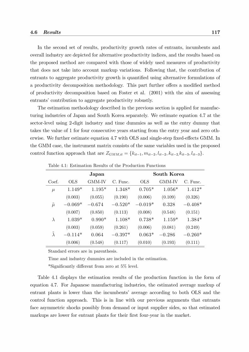
4.6 Results 117
In the second set of results, productivity growth rates of entrants, incumbents and
overall industry are depicted for alternative productivity indices, and the results based on
the proposed method are compared with those of widely used measures of productivity
that does not take into account markup variations. Following that, the contribution of
entrants to aggregate productivity growth is quanti�ed using alternative formulations of
a productivity decomposition methodology. This part further o¤ers a modi�ed method
of productivity decomposition based on Foster et al. (2001) with the aim of assessing
entrants�contribution to aggregate productivity robustly.
The estimation methodology described in the previous section is applied for manufac-
turing industries of Japan and South Korea separately. We estimate equation 4.7 at the
sector-level using 2-digit industry and time dummies as well as the entry dummy that
takes the value of 1 for four consecutive years starting from the entry year and zero oth-
erwise. We further estimate equation 4.7 with OLS and single-step �xed-e¤ects GMM. In
the GMM case, the instrument matrix consists of the same variables used in the proposed
control function approach that are ZGMM;it = fkit�1;mit�2; lit�2; kit�2;kit�3; lit�3g.
Table 4.1: Estimation Results of the Production Functions
Japan South KoreaCoef. OLS GMM-IV C. Func. OLS GMM-IV C. Func.
� 1.149* 1.195* 1.348* 0.705* 1.056* 1.412*
(0.003) (0.055) (0.190) (0.006) (0.109) (0.326)
~� �0.069* �0.674 �0.520* �0.019* 0.328 �0.408*(0.007) (0.850) (0.113) (0.008) (0.548) (0.151)
� 1.039* 0.990* 1.108* 0.738* 1.159* 1.384*
(0.003) (0.059) (0.261) (0.006) (0.081) (0.249)~� �0.114* 0.064 �0.397* 0.063* �0.286 �0.260*
(0.006) (0.548) (0.117) (0.010) (0.193) (0.111)
Standard errors are in parenthesis.
Time and industry dummies are included in the estimation.
*Signi�cantly di¤erent from zero at 5% level.
Table 4.1 displays the estimation results of the production function in the form of
equation 4.7. For Japanese manufacturing industries, the estimated average markup of
entrant plants is lower than the incumbents� average according to both OLS and the
control function approach. This is in line with our previous arguments that entrants
face asymmetric shocks possibly from demand or input supplier sides, so that estimated
markups are lower for entrant plants for their �rst four-year in the market.

118 Price-Cost Markups and Productivity Dynamics of Entrant Plants
According to the control function approach, the degree of total returns to scale estimate
is also lower for entrants. If one believes that the optimality condition given in equation
4.4 holds for the capital input, then we can de�ne the identity � = ��sMit + s
Lit + s
Kit
�,
so that it is possible to retrieve an estimate of total input expenditures to revenue ratio
(pro�t margin) that is 1:108=1:348 = 0:822 for incumbents and 0:711=0:828 = 0:859 for
entrants based on the control function approach estimates for the Japanese manufactur-
ing industries. However, as we noted before, our speci�cation does not necessitate the
static optimality condition for capital input, and the degree of returns to scale parameter
estimates may take a value irrespective of this markup and cost to pro�t ratio relationship.
The OLS estimates of average incumbents�markup (�) and returns to scale (�) are
particularly low in comparison to the results obtained from the other approaches. This
is mainly because the input expenditure shares in revenue is negatively correlated. Con-
versely, the factors of production are expected to be positively correlated with unobserved
productivity, but capital input enters in the joint term, sMit (�mit ��kit)+ sLit (�lit ��kit),with a negative sign. Thus, the possible negative correlation of productivity with sMit , s
Lit
and ��kit cause the OLS estimates of � to be biased downwards. In addition, the coef-�cient estimate of the markup variation (~�) is smaller in absolute value in the OLS case.
This indicates that the degree of downward bias in the OLS markup estimates is larger
for incumbents than entrants. Therefore, the negative correlation between unobserved
productivity and input expenditure shares is weaker for entrant �rms, possibly due to
previously mentioned demand side e¤ects involved in nominal input to output ratios.
The reliability of the standard GMM estimates with an instrument matrix consisting
of lagged inputs depends on the degree of persistence in productivity over time. As
argued in Levinsohn and Petrin (2003), if productivity is signi�cantly serially correlated,
the previous periods�input usage would be still correlated with the error term, where the
error term contains unobserved productivity component in the standard GMM and OLS
speci�cations. Therefore, in the presence of questionable instruments such as previous
periods�input usages, the GMM estimates would be far from the estimates obtained by
the control function approach. This is indeed the case according to the results reported in
Table 4.1, so that the coe¢ cient estimates for incumbents are signi�cant and the values
are close to the OLS estimates, but entrants�variations in terms of markup and returns
to scale are insigni�cant in the Japanese manufacturing industries.
The picture depicted on the right-hand side of Table 4.1 for South Korea is not very
di¤erent from the results obtained for Japanese manufacturing industries. Accordingly,
the OLS and the control function estimates of entrants�markup variation are signi�cantly
negative. The OLS estimates of incumbents�markup and the degree of returns to scale

4.6 Results 119
are lower than the control function estimates possibly due to the endogeneity problem.
In addition, entrants�total returns to scale variation is estimated to be positive with the
OLS but negative with the control function approach. As in Japan, we do not retrieve
signi�cant coe¢ cient estimates for entrants�variation for South Korea from the standard
GMMmethod with lagged inputs as instruments. Assuming capital to be a static input of
production, pro�t margin (sMit +sLit+s
Kit ) estimates based on the control function approach
are 1:384=1:412 = 0:98 for incumbent and 1:124=1:004 = 1:12 for entrant plants in South
Korean manufacturing industries.
So far, we conclude that price-cost markups involving unobserved price e¤ects are
lower for entrant plants and higher for incumbents in both Japanese and South Korean
manufacturing industries. The next step is to �nd out whether the productivity growth
contribution of entrants is a¤ected by taking into account plant-level markup variations.
The next section approaches the question from two di¤erent perspectives. We �rst com-
pare the annual productivity growth rates for alternative productivity indices. Second,
we decompose productivity growth for alternative productivity measures including the
proposed one that is adjusted to entrants�markup variation. The decomposition method-
ology is based in Foster et al. (2001), but we also develop a discussion over their method
and applied two alternative decomposition formulations.
4.6.1 Entrants�Productivity Growth
This section investigates whether entrants�average productivity growth rates are raised
when we take into account their markup variation from incumbents. We calculate entrants�
productivity growth rates using three alternative productivity indices. The �rst one is the
total factor productivity index (TFP-markup) that is adjusted to the markup variation
between entrants and incumbents. The other two productivity indices are the standard
measures that are the labor productivity as the ratio of de�ated revenues to total work-
ing hours and the total factor productivity (TFP) estimated by Levinsohn and Petrin
(2003) algorithm.8 Therefore, we compare the productivity growth rates based on the
8In the estimation of the standard TFP, we utilize the code levpet that is provided by Levinsohn et
al. (2004) and applies the Levinsohn and Petrin (2003) algorithm in Stata.

120 Price-Cost Markups and Productivity Dynamics of Entrant Plants
two standard measures with those form the markup-adjusted total factor productivity
index.9
In the estimation of standard TFP growth rates by Levinsohn and Petrin (2003), we
consider a Cobb-Douglas type production function. The growth rates are calculated by
considering log di¤erences, and the industry weighted average of the growth rates are
calculated by using output shares (wit) in the formulation of the weights that is �wit =
(wit + wit�1) =2. In order to take the average of the growth rates of TFP-markup, we also
consider two-year averaged output shares as weights, while average labor productivity is
weighted by labor shares in total amount of labor employed in an industry in terms of
working hours.
Besides comparing the results of these two alternative measures of TFP is our main
aim in this section, labor productivity is of particular importance since in its calculation,
we use total working hours employed by a plant in a given year that does not contain
plant-level input price e¤ects. Once more, entrants are de�ned to be the plants that are
in their �rst four years in the market.
Table 4.2: Annual Growth Rates (%) in the Manufacturing Sectors
Japan South KoreaEntrant Inc. Industry Entrant Inc. Industry
Labor Prod. 4.2 5.0 5.0 7.0 7.3 7.3
TFP �3.3 0.2 0.1 �1.6 �0.7 �0.8TFP-markup 2.6 0.8 0.8 �0.4 �3.1 �3.0Output 5.1 3.4 3.4 28.9 11.0 11.2
Labor 0.2 �2.0 �1.9 12.7 1.0 1.3
Labor is measured by annual working hours and output is the
revenues de�ated by 2-digit industry PPI.
Labor prod. is calculated by the ratio of output to labor input.
Table 4.2 presents the annual average growth rates of labor productivity, TFP, TFP-
markup, output and labor in manufacturing sectors of Japan and South Korea. The
results are displayed for three plant groups separately, that are entrants, incumbents and
9A productivity index that is adjusted to average industry markups, but not entrants markup variation,
also can be considered in the set of compared productivity measures. We can retrieve such an index by
applying our own methodology without introducing an entrant dummy into the �nal estimating equation.
However, it is straightforward that the productivity growth rates for entrant plants would be lower in
the case of constant markup than varying markups. This is because the dependent variable minus the
�tted values of the regression (excluding the control function) would be lower for entrants in the constant
markup case.

4.6 Results 121
the entire industry. According to the left-hand side of the table, the growth rates of labor
productivity and standard TFP is on average lower for entrants than incumbents in Ja-
panese manufacturing industries. We calculate a yearly average of 5% labor productivity
growth and 0.2% TFP growth for incumbents, while entrants�TFP growth is negative
with -3.3% and labor productivity growth rate is slightly lower than incumbents�average.
In contrast, the productivity growth rates that are measured by the proposed method
(TFP-markup) are much higher for entrants (2.7%) than those for incumbents (0.7%) in
the Japanese manufacturing sector. Moreover, the annual average growth rates of output
(5.1%) and labor (0.2%) are signi�cantly higher for entrants, while incumbents� labor
input growth is negative. Therefore, Table 4.2 provides evidence, to some degree, on the
fact that there is a signi�cant reallocation of labor from incumbents to possibly more
productive entrant plants in the Japanese manufacturing sector.
The right-hand side of Table 4.2 presents the �ndings for the South Korean manu-
facturing sector, which are similar to the Japanese case. Entrants�average productivity
growth is lower than that of incumbents according to labor productivity. The stand-
ard total factor productivity growth rates are negative for both entrants and incumbents
with entrants having the worst TFP growth performance. The TFP-markup also indic-
ates that total factor productivity growth is negative for each plant group in the South
Korean manufacturing industries, but entrants have higher productivity growth rates than
incumbents.
We �nd overall negative TFP growth in the South Korean manufacturing sector (-0.8%
TFP growth and -3% TFP-markup growth), but the growth rates of output and labor are
positive and higher than the respective rates in Japan. Although analyzing growth and
productivity trends in Japan and South Korea are not the main purpose of this study,
our �ndings are in line with the argument that South Korea is experiencing higher output
growth rates mainly due to expansionary growth in inputs instead of TFP, while Japan�s
output growth rates seem to rely heavily on growth in productivity.

122 Price-Cost Markups and Productivity Dynamics of Entrant Plants
Figure 4.1: Annual Productivity Growth (%) in Japanese Manufacturing Sector
1988 1990 1992 1994 1996 1998 2000 2002 20045
0
5
10La
bor P
rod.
entrantsindustry
1988 1990 1992 1994 1996 1998 2000 2002 2004864202
TFP
1988 1990 1992 1994 1996 1998 2000 2002 2004202468
TFP
mar
kup
Figure 4.1 provides a closer look at the productivity growth performances of manu-
facturing plants operating in Japan. The overall industry productivity growth patterns
with respect to TFP and TFP-markup indices are rather similar with joint downturns in
years 1993, 1996, 1998 and 2001, and booms in 1995, 1997, 2000 and 2003. Both TFP
indices re�ect less volatile patterns in comparison to labor productivity, and indicate that
the Japanese manufacturing sector follows an increasing total factor productivity growth
time path over the period 1987-2005.
The standard TFP measure displays that entrants�productivity growth follows a time
path with peaks and downturns similar to the overall industry pattern. Conversely,
entrants�TFP-markup trend is rather cyclical in comparison to the industry average.
In particular, entrants�TFP-markup growth rates seem to be highly and positively cor-
related with entrants�labor productivity growth. This is possibly because adjusting the
production function estimates to markups as well as �rm-level factor elasticity variation
leads entrants�production technology to be measured more labor intensive, which would
be meaningful for new �rms that possibly face stricter �nancial limitations to invest
in more capital intensive production methods. However, the standard measure of TFP
attaches constant factor elasticities to all �rms in an industry, so that the production
methods used by entrants and incumbents are assumed to be the same.

4.6 Results 123
The e¤ect of the East Asian �nancial crisis reveals itself with signi�cant downturns
in the three listed productivity measures in 1998. In particular, entrant plants seem to
be more prone to such aggregate downturns, probably because new �rms that are in the
start-up phase and face adverse demand shocks may cut back new investments or exit the
market more easily in case of a stricter �nancial environment. However, what makes this
picture more interesting for our purpose is the di¤erences in the speed of the recovery of
entrants�productivity growth rates for the alternative indices. According to the TFP-
markup, the slowdown in the productivity growth rates of entrants in 1998 is recovered
a year after, followed by a noticeable peak in 2000. This is in line with the well-known
cleansing e¤ect of recessions (Caballero and Hammour, 1994) by which the market clears
out ine¢ cient units and creates new pro�t opportunities for potential entrants. However,
the standard TFP indicates that entrants�productivity growth rates turn back pre-crisis
levels only after 2001. We attribute the di¤erence of the recovery periods observed in TFP
and TFP-markup also to the assumption of constant factor elasticity in the estimation
of TFP that is abandoned in TFP-markup. Namely, producers may react to changing
conditions by altering their production technology, for instance shifting from capital to
labor intensive production, that is not accounted for in the measurement of the standard
TFP.
Figure 4.2: Annual Productivity Growth (%) in S. Korean Manufacturing Sector
1988 1990 1992 1994 1996 1998 2000 2002 20040
5
10
15
Labo
r Pro
d.
entrantsindustry
1988 1990 1992 1994 1996 1998 2000 2002 2004
64202
TFP
1988 1990 1992 1994 1996 1998 2000 2002 2004
5
0
5
TFP
mar
kup

124 Price-Cost Markups and Productivity Dynamics of Entrant Plants
Figure 4.2 displays the time paths of annual labor and total factor productivity growth
rates in the South Korean manufacturing industries. Labor productivity growth rates
are always positive during the sample period, while the total factor productivity growth
average of the sector is mostly negative according to both TFP measures. Therefore, the
relative share of labor in production decreases, so that labor productivity growth outpaces
TFP growth in South Korean manufacturing industries.
Entrants�productivity performance is higher than incumbents with respect to TFP-
markup, while new �rms�productivity growth rates are on average lower according to the
other productivity measures. However, during the last 5 years of the sample period, the
labor productivity growth rates are also higher for entrants than incumbents. In addition,
the TFP-markup indicates that the gap between entrants�and incumbents productivity
growth rates is larger for the last �ve-year period. Therefore, the productivity trend in
South Korea seems to be changed after East Asian �nancial crisis especially for entrant
�rms whose relative productivity performance is signi�cantly improved.
The above analysis was based on average annual growth rates in manufacturing sectors
of Japan and South Korea where entrants were classi�ed as the producers that are observed
in the �rst four years of their life time. However, more can be said by avoiding the four-
year restriction in the de�nition of entrants and taking into account the level form of
productivity. The next section approaches the aggregation and accounting issues by taking
into account these features through a methodology of productivity growth decomposition
developed in Foster et al. (2001).
4.6.2 Decomposition of Productivity Growth
The Foster-Haltiwanger-Krizan (FHK) productivity decomposition method (Foster et al.,
2001), provides an intuitive accounting of entrants�productivity growth contribution; in
particular, the contributions can be considered over time intervals at varying duration.
The FHK de�nes an entrant as the plant that is absent from the industry in the �rst year
of the time interval but present in the last year. For instance, if the time interval is 10
years, a 9-year old �rm is considered an entrant in year 10. Similarly, a plant that enters
into the market one year before the starting date of the time interval is considered an
incumbent.
The FHK method requires not the growth rate but the level form of productivity, for
which we need to introduce further assumptions into our productivity estimation meth-
odology. Our production function speci�cation in the previous parts was in terms of �rst
di¤erences, mainly because we do not want to restrict the estimation to a particular type

4.6 Results 125
of production function. In case one assumes a Cobb-Douglas type production function,
it is possible to derive the same functional form in equation 4.7 in terms of levels as in
the original Hall�s approach. Therefore, we can retrieve a productivity index based on
the proposed method, which we continue to call TFP-markup, by considering the level
forms of output and inputs with the estimated coe¢ cients for markups and the degree of
returns to scale.
As in the previous part, we decompose aggregate productivity growth using three
di¤erent productivity measures which are TFP-markup, labor and standard total factor
productivity indices. The decomposition necessitates the calculation of aggregate pro-
ductivity that is the weighted average of plants� productivity levels, where labor and
output shares are used as the weights (wit).
Equation 4.14 is the formula of FHK decomposition.
���t =Xi2C
wit�k��it +Xi2C
�wit��it�k � ��t�k
�+Xi2C
�wit��it (4.14)
+Xi2N
wit��it � ��t�k
��Xi2X
wit�k��it�k � ��t�k
�In equation 4.14, C, N and X represent the sets of all plants, entrants and exiters
respectively, where ���t = ��t� ��t�k represents log di¤erenced aggregate productivity, and�i�s are the plant level productivity draws.
The �rst term in the FHK formula is the within component that measures �rms�pro-
ductivity performance holding their market shares constant and equal to initial level, so
that it provides insights on the degree of �rm restructuring or deterioration. The second
term is the between component measuring the aggregate productivity growth e¤ects of
relative changes in plants� labor or output shares which can be interpreted as the pro-
ductivity e¤ects of the allocation across establishments. The third term is the covariance
between productivity and market share that is referred to the cross term. The cross term
is positive, if the expanding (shrinking) production units in terms of their market share
also experience positive (negative) growth in their productivity over the period whose
span is represented by k in the formulation. The forth term, which is the main concern of
this part of the study, is the entry component that accounts the productivity contribution
of entrants weighted by their shares in total. The last term on the right-hand side is
the exit component that re�ects whether exiting plants during the period between t and
t� k have lower productivity levels than the industry average which accounts for exiters�contribution to productivity growth.
A closer look at the entry contribution of the FHK decomposition reveals that the
productivity of entrants at time t is compared with the productivity average at time t�k.

126 Price-Cost Markups and Productivity Dynamics of Entrant Plants
This means that the entry component of the FHK is sensitive to a change in the overall
productivity level of the industry that may be regardless of entrants�own productivity
performance. For instance, if the industry exhibits considerable productivity growth after
the initial time point (t � k), a new producer that enters in time t may have lower pro-ductivity relative to incumbents�average in time t. However, time-t entrants�productivity
may still be much higher than time t � k�s average, so that the entry component wouldindicate high contribution to aggregate productivity growth.
Brown and Earle (2008) (BE) account the e¤ect of average industry growth on the
entry term of the FHK method, and decompose the entry component into two parts that
are displayed in the below formula.Xi2N
wit��it � ��t�k
�=Xi2N
wit���t � ��t�k
�+Xi2N
wit��it � ��t
�(4.15)
The BE extension separates the entry term of the FHK decomposition into two com-
ponents that are the growth due to overall industry trend (referred to agg. growth e¤ect in
the following tables) and entrants�own productivity performance, where the latter com-
ponent is the net contribution of entrants (referred to the net entry component). Thus, if
the industry experiences a positive (negative) overall productivity growth, the BE exten-
sion would re�ect a net entry contribution that is lower (higher) than the original entry
component of the FHK.
In case average industry productivity growth rate is di¤erent from zero, this can be,
however, due to entrants�own productivity contribution. Namely, the group of �rms that
enter into the market between t and t� k would be an important driving force of aggreg-ate productivity growth that would still remain a bias in the BE extension. Therefore,
the �rst term in the BE extension that accounts for aggregate growth would capture a
part of entrants�contribution which may distort the second term, namely, the net entry
component in both ways depending on the sign of entrants�contribution. Therefore, we
further revise the BE extension in order to calculate the pure entry contribution in the
below formula.Xi2N
wit��it � ��t�k
�=Xi2N
wit
���It � ��t�k
�+Xi2N
wit
��it � ��
It
�(4.16)
In equation 4.16, ��It represents the weighted productivity average of the plants except
the ones that enter into the market during the period of k. Therefore, the �rst term on the
right-hand side of the revised BE identity represents the productivity growth performance
of plants, which are not entrants, weighted by entrants�share. The second term is the pure
entry e¤ect that measures entrants�productivity contribution by taking the productivity
average of all other �rms in the industry as the benchmark.

4.6 Results 127
We decompose the entry contribution from aggregate productivity growth in the South
Korean and Japanese manufacturing industries using the three alternative decomposition
formulations. We set the span of decomposition to two di¤erent values k = 5 and 10,
and decompose productivity growth for every period and 2-digit manufacturing industry
separately. While averaging the components over 2-digit industries, we use the industry
shares in overall manufacturing sector as weights. Then, we take the unweighted average
of the components over time to reach the �nal statistics reported in Table 4.3. Lastly,
industry-level log di¤erenced productivity (���t) and each entry component is multiplied
by 100, so that the total growth term (Tot. Gr.) is in percentage form.
Table 4.3: Decomposition of Productivity Growth (%)
FHK BE Extension Revised BE Tot. Gr.
Entry Ag. Gr. Net Ent. Ag. Gr. Net Ent. ���t�100Japan5-year Lab. Pr. �0.15 0.56 �0.71 0.58 �0.73 19.20
TFP 1.91 0.03 1.89 0.01 1.90 2.84
TFP-m 13.82 0.80 13.02 �0.34 14.16 3.53
10-year Lab. Pr. 0.78 2.49 �1.71 2.53 �1.75 41.77
TFP 3.81 0.14 3.67 0.07 3.74 6.24
TFP-m 12.47 0.85 11.62 �0.69 13.16 4.48
South Korea5-year Lab. Pr. 1.68 2.20 �0.52 2.12 �0.44 44.22
TFP 0.12 �0.29 0.41 �0.24 0.36 �2.83TFP-m 18.47 1.84 16.63 �1.96 20.43 �4.29
10-year Lab. Pr. 8.60 10.79 �2.19 10.67 �2.07 105.20
TFP 0.69 �0.65 1.34 �0.60 1.28 �5.78TFP-m 20.46 �0.10 20.56 �5.86 26.32 �23.52
Table 4.3 displays the results of entrants�contribution to productivity growth analysis
through the FHK decomposition with three alternative entry component formulations.
As before, TFP represents the standard total factor productivity, Lab. Pr. stands for the
labor productivity, and the TFP-m is the index retrieved from the proposed method that
takes into account entrants�markup variation. The column titled as FHK represents the
entry component of the original method, and the following columns display the results of
the extensions in which the original entry component is separated into aggregate growth
and net entry components.

128 Price-Cost Markups and Productivity Dynamics of Entrant Plants
The upper part of Table 4.3 displays the components of decomposed productivity
growth in the Japanese manufacturing sector for 5 and 10-year spans respectively. Based
on a 5-year window, the average entry contribution to labor productivity growth is neg-
ative for all three decomposition formulations. For a 10-year window, the FHK entry
component of labor productivity growth is positive mainly due to increase in the industry
average growth rates for longer time spans. Namely, when we subtract the aggregate
growth e¤ect from the FHK�s entry component, the resulting net entry contribution to
labor productivity is negative with both BE and revised BE methods.
In contrast, the entry contribution to standard TFP growth is positive for all de-
composition methods, and increases signi�cantly for the 10-year window in the Japanese
manufacturing industries. This result is in line with the fact that with the standard TFP
measure, entrants�contribution to productivity growth is signi�cantly positive and higher
in the long run, but their overall productivity performance may be poor during their �rst
years in the market.
Entrants�contribution to the Japanese manufacturing sector�s productivity growth is
the highest, when we consider the TFP-m as the productivity measure of the analysis.
Although aggregate total factor productivity growth in terms of both TFP and TFP-m is
rather low relative to labor productivity growth (the 5-yearly growth is around 3%, and
the 10-yearly growth is around 5% according to both TFP and TFP-m), calculated entry
contributions with the TFP-m are much higher than those based on labor productivity.
The results further show that the value of the entry component based on TFP-m is
approximately the same among alternative formulations and time spans indicating that
the TFP-m does not underestimate the role of entrants in the Japanese industry dynamics
even for shorter time intervals.
The overall picture depicted for the South Korean manufacturing industries is not
signi�cantly di¤erent from the Japanese case. The entrant plants�contribution to pro-
ductivity growth is highest when we consider the TFP-m as the productivity measure. The
net entry contribution to labor productivity growth is negative according to the BE and
revised BE methods, whereas the original entry component of the FHK method indicates
a positive contribution to labor productivity growth for both 5 and 10-year intervals.
Entrants� role in labor productivity dynamics signi�cantly di¤ers across alternative
decomposition techniques highlighting the importance of extracting the aggregate growth
e¤ect from the original entry component of the FHK decomposition. Moreover, the net
entry contributions of the BE and revised BE methods also vary in the decomposition of
TFP-m growth for the South Korean manufacturing sector mainly due to the di¤erence
between observed productivity performances of entrants and incumbents. In other words,
4.7 Conclusion 129
since incumbents are experiencing negative and very low productivity growth rates in
South Korea, the aggregate growth e¤ect in the revised BE is lower than the original BE
extension, so that net entry contribution of the revised BE is signi�cantly higher in terms
of TFP-m.
4.7 Conclusion
The analysis of �rm-level productivity is an important step to understand how producers
process inputs to turn them into output. Besides providing insights into cross-industry
or -country di¤erences in �rm behavior, the economics of productivity signi�cantly con-
tributes to the knowledge of economic growth and microeconomic restructuring that is
ongoing in an economy. However, although the theoretical concept of productivity is
rather well established, its measurement in practice is still ambiguous, especially when
the quantities of inputs and outputs are not directly observable.
Even though �rms�productivity measures are ideally computed by the quantities of
inputs and outputs, the lack of �rm-level prices or quantities entail using revenues and
input expenditures in the measurement of productivity. However, empirical evidence
shows that, revenue-based productivity indices actually involve external factors that are
generated regardless of the technical e¢ ciency in production process. These factors can
be in the form of adverse shocks from demand or input suppliers�sides and show up in
the form of unobserved idiosyncratic price-cost markups in productivity indices based on
nominal input and outputs.
In real industries, there is some degree of imperfect competition, so that price-cost
markups generally di¤er across �rms. Therefore, de�ating �rm-level revenues or input
expenditures by aggregate price indices would not be su¢ cient to eliminate �rm speci�c
price e¤ects. This leads a productivity index based on de�ated revenues to be a distorted
measure of productivity, especially if the markup variation among �rms has a systematic
pattern. For instance, newly created production units face asymmetric shocks that prevent
entrants to charge markups as high as incumbents during the start-up phase. If this is
the case, then revenue-based productivity measures may not provide reliable information
on the productivity performance of entrant �rms.
In this chapter, we provide empirical support that entrants set on average lower
markups than incumbents in the Japanese and South Korean manufacturing industries.
Assuming that plants are price takers in the input market, our �ndings can be interpreted
as a sole result of idiosyncratic demand shocks. However, we do not restrict ourselves to

130 Price-Cost Markups and Productivity Dynamics of Entrant Plants
a speci�c market condition or a production relation, so that the adverse shocks faced by
entrants may well originate from the side of input suppliers.
In addition to providing insights on the importance of within-industry heterogeneity
in plants�pricing behavior, our approach supplies a productivity index that is adjusted to
the markup variation of entrants as well as overall industry markups that are not equal to
one. The estimation methodology further controls for a possible correlation between two
unobserved components, markups and productivity, as well as the endogeneity of input
usage to production by introducing a control function approach. In the concluding part of
the study, we could, therefore, consistently assess entrants�role in aggregate productivity
growth, and compare the results with the ones derived from alternative productivity
indices that are widely-used in the recent literature.
Our results show that according to standard labor and total factor productivity meas-
ures, the average productivity growth rates of entrant plants in their �rst four years are
lower than incumbents in both Japanese and South Korean manufacturing sectors. How-
ever, the total factor productivity index retrieved by controlling for the markup variation
of entrants indicates that entrant plants�productivity growth rates are signi�cantly higher
than those of incumbents.
In the next step, using alternative productivity growth decomposition frameworks, we
calculate the productivity contribution of entrants for 5- and 10-year time intervals. The
results demonstrate that entrants� contribution to productivity growth is signi�cantly
higher, when we account for their markup variation in the estimation of productivity.
Moreover, the calculated productivity contribution of entrants are not sensitive to al-
ternative time spans according to markup-adjusted productivity index, whereas standard
measures re�ect signi�cantly lower entrants�contribution as we shorten the time interval.
Our �ndings highlight the importance of distortionary price e¤ects in the measurement
of productivity at the micro-level. This is especially crucial if the variation of demand
side factors involved in productivity indices has a non-random pattern. Thus a particular
group of producers�production performance would be evaluated inaccurately, if we ignore
their variation from the industry average. In this study, we only consider entrants as
the group of plants that deviates from overall industry dynamics, but one can rely on
alternative classi�cations such as domestic and foreign, private and state-owned �rms for
which pricing behaviors possibly di¤er even within narrowly de�ned industries. Therefore,
�rm-level productivity analysis vitally needs productivity indices that are controlled for
micro-level price variations, especially when the aim of the analysis is to compare the
productivity performances of �rm groups within the same industry.

4.8 Appendix 131
4.8 Appendix
Construction of Variables and Detecting the Outliers
In addition to the input and output variables discussed in the main text, the estima-
tion procedure further requires to obtain the respective factor expenditure shares in total
revenues. In the original dataset, only total hours worked as labor input, price-adjusted
capital, material expenditures and revenues are reported together with each input�s ex-
penditure share in total input expenditures for every plant and time period. However, as
it is explained in Fukao et al. (2009), expenditures on material inputs and revenues are
de�ated with the same price index (2-digit industry level PPI) which enables us to retrieve
the input expenditure to revenue ratio for labor input conveniently in the following way.
The nominal material expenditure to revenue ratio could be calculated by the ratio
of the de�ated material expenditures to de�ated revenues ratio, since both variables are
adjusted by the same price index. Moreover, because we have a variable that represents
each inputs�expenditure share in total input expenditures, that is zJit where J 2 fM; Lg,then total expenditures on labor to revenues ratio can be retrieved from the following
formula that is irrespective of the value of total costs.
witLitpitQit
=citMit
pitQit
zLitzMit
(A.1)
The above formula consist of plant-level variables where Qit represents the quantity
of output, pit is the output price, wit and cit are the input prices for labor (Lit) and
materials (Mit) respectively. It is worth mentioning that in the dataset, the capital�s cost
share in total input expenditures is also reported, where capital�s user cost is calculated
through an approximation over variables such as interest and depreciation rates, capital
price de�ators that results in a �xed capital input price value which is the same for all
plants in a 2-digit industry. Therefore, even though it is technically possible to retrieve a
capital expenditures to revenue ratio for each plant and time period in the same manner,
we already assumed and stated in the main text that the user cost of capital is not
observable and subject to possible errors in its approximation. Thus, we do not use its
respective share in the proposed analysis.
When detecting extreme values, we �rst estimate the production functions through the
proposed algorithm by using the full sample. Then, we re-center the retrieved TFP index
of the full sample by extracting the mean of each 2-digit industry and time period from
the plant-level TFP in logarithms. In the next step, for each year, we rank the �rms ac-
cording to their re-centered productivity draws for the group of entrants and incumbents

132 Price-Cost Markups and Productivity Dynamics of Entrant Plants
separately. Lastly, within each group, we detect the �rm-time observations that are 4:2
standard errors far away from the mean as the outliers. This process leads to the deletion
of approximately between 1% and 2% of total number of �rm-time observations for each
country. In the South Korean �rst di¤erenced dataset we have 13139 �rm*time obser-
vations, and in the Japanese �rst di¤erenced dataset there are totally 28995 �rm*time
observations.
App. Table 4.1: Summary Statistics (in 2000�s prices)
Output Labor Materials Capital
Levels Jap. yen man-hours Jap. yen Jap. yen
Japan
Mean 108802621 3668371 88415033 45356663
Std 360405257 9797515 304745977 155806339
S. Korea
Mean 11310196 2309099 32710523 11310196
Std 76825891 8108075 236974182 76825891
Growth Rates
Japan
Mean 0.019 �0.022 0.017 0.024
Std 0.141 0.108 0.144 0.151
S. Korea
Mean 0.119 0.014 0.127 0.173
Std 0.337 0.262 0.345 0.642

4.8 Appendix 133
App. Table 4.2: Entry and Exit Rates (%) in Japanese Industries
Code Entry R. Exit R. C.V. Labor C.V. Materials #Firms
6 1.61 0.37 1.65 2.17 138
7 0.01 0.08 1.27 1.29 27
8 1.08 0.42 1.34 1.31 43
9 2.20 1.00 0.93 1.11 9
10 1.67 0.49 0.92 0.96 11
11 0.47 2.62 1.27 1.47 34
12 1.69 0.11 1.99 2.54 26
13 0.58 0.87 1.41 1.70 202
14 0.14 1.35 0.91 1.31 10
15 8.28 0 0.63 0.72 3
16 0.73 1.02 1.50 1.98 79
17 0.50 0.77 2.29 2.14 104
18 2.01 1.09 1.48 1.78 88
19 0.57 0.60 2.41 2.92 231
20 0.64 0.34 2.96 3.51 232
21 0.60 0.25 2.08 3.08 107
22 0.46 0.85 0.97 1.51 29
23 1.06 0.48 1.13 1.40 48
24 1.15 0.23 1.62 1.72 62
The entry and exit rates are the annual averages based on
the plants�labor shares.
"C.V." represents the coe¢ cient of variation.
"#Firms" stands for the average number of �rms in the industry.
"Code" is the respective 2-digit industry codes.

134 Price-Cost Markups and Productivity Dynamics of Entrant Plants
App. Table 4.3: Entry and Exit Rates (%) in S. Korean Industries
Code Entry R. Exit R. C.V. Labor C.V. Materials #Firms
6 0.71 0.00 1.23 1.46 48
7 0.10 0.01 1.10 1.12 23
8 0.68 0.17 1.03 1.85 25
9 0.10 0 0.57 0.29 4
10 0.52 0 1.12 0.87 7
11 0.33 0 1.08 1.43 30
12 6.04 0.56 1.29 1.78 29
13 1.22 0.02 1.91 2.68 116
14 0.11 0 1.45 1.89 4
15 0.55 0 1.08 0.53 5
16 0.07 0 1.11 1.61 28
17 0.21 0.07 3.18 3.44 63
18 0.99 0 2.49 3.43 28
19 2.00 0.10 1.48 2.70 52
20 1.87 0.06 4.64 5.33 163
21 0.44 0 3.39 3.57 51
22 1.04 0 1.34 1.43 6
23 1.04 0.05 2.62 3.26 19
24 1.71 0 1.50 2.02 20
The entry and exit rates are the annual averages based on
the plants�labor shares.
"C.V." represents the coe¢ cient of variation.
"#Firms" stands for the average number of �rms in the industry.
"Code" is the respective 2-digit industry codes.

4.8 Appendix 135
App. Table 4.4: Manufacturing Industries Used in the Analysis
Industry Code De�nition of the Manufacturing Industry
6 Food and kindred products
7 Textile mill products
8 Apparel
9 Lumber and wood
10 Furniture and �xtures
11 Paper and allied
12 Printing publishing and allied
13 Chemicals
14 Petroleum and coal products
15 Leather
16 Stone clay glass
17 Primary metal
18 Fabricated metal
19 Machinery non-electrical
20 Electrical machinery
21 Motor Vehicles
22 Transportation equipment and ordnance
23 Instruments
24 Rubber and misc plastics

Chapter 5
Conclusions
Unobservable prices at the micro-level constitute a major problem in the �rm-level pro-
ductivity analysis. Economists often de�ate �rm-level nominal data using aggregate-level
price indices, which introduces the implicit assumption of homogenous prices or per-
fect competition into the underlying structural model. Calculated productivity based on
revenues and expenditures, therefore, involve price e¤ects that may highly distort the in-
dicative quality of the index. This dissertation develops micro-oriented empirical models
to analyze �rm dynamics, productivity and competition while, in most cases, attempting
to control for the possible bias due to unobserved �rm-level price variation.
The second chapter explores entry-exit, factor allocation and productivity dynamics
in the manufacturing and business services sectors of Ukraine for the period 2001 to 2007.
The period under study was one of the rapid growth at the level of the total economy,
while the main sectors have undergone considerable churn and reallocation among �rms
and workers. The �ndings imply that the large-sized establishments in the manufacturing
and state-owned enterprises in the business services sectors substantially dominate the
�rm dynamics in Ukraine. However, the analysis of productivity displays dramatically
di¤erent pictures for the two main sectors, so that large �rms in the manufacturing are as
productive as �rms in the other size groups, while the large and mostly state-owned �rms
in the business services perform rather poorly in comparison to small-sized private estab-
lishments. The prevalent state ownership in the business services considerably distorts
the functioning of the creative destruction process and the e¢ ciency in factor alloca-
tion, which holds back the productivity performance and deteriorates the quality of the
microeconomic restructuring of the economy.
The third chapter analyses the relationship between the selected measures of compet-
ition and the actual intensity of the interaction in the product market under the presence
of frictions. The chapter is separated into two parts where the �rst part consists of a
138 Conclusions
theoretical study that compares the industry-level price-cost margin and pro�t elasticity
within a model of monopolistic competition where the degree of substitutability among
the product varieties is the determinant of the level of �rm-to-�rm interaction. The
second part studies the empirical performances of the indices through a panel of manu-
facturing �rms operating in Ukraine during 2004-2007. Particular attention is devoted
to the method of pro�t elasticity that is a theoretically robust measure of competition.
However, this chapter advances the literature by developing an alternative approach to
measure the elasticity of pro�ts to productivity that relies on the structural estimation
of the industry production functions. The estimation methodology is based on Levinsohn
and Melitz (2004) and takes into account unobservable prices by introducing demand side
into the structural model. Moreover, the methodology retrieves elasticity of substitution
estimates at the industry-level jointly with the �rm-level total factor productivity index.
The �ndings imply that while the proposed method to measure pro�t elasticity provides
a robust indicator of competition, the price-cost margin and the standard pro�t elasticity
fail to indicate the true level of competition especially when the intensity of interaction
among �rms is relatively low.
The fourth chapter of this study derives a production function estimation methodo-
logy that retrieves the markup estimates separately for the entrants and incumbents, and
provides a productivity index that is adjusted to the markup variation of entrant plants.
The methodology takes into account the endogeneity of inputs to unobserved productivity
by extending the control function approach of Levinsohn and Petrin (2003). In the �rst
step, the proposed control function speci�cation is introduced into Hall�s (1988) structural
model which also accounts for the variation in production factor elasticities. The estim-
ation routine applied in this section does not require observing prices at the micro-level,
and the implications can be tested for widely available �rm- or plant-level datasets. The
predictions are examined using a plant-level data from the manufacturing industries in
Japan and South Korea, and the �ndings show that entrants set lower markups than in-
cumbents in both countries. Moreover, the contribution of the entrant plants to aggregate
productivity growth is calculated to be signi�cantly higher with the adjusted productivity
measure than those based on standard labor and total factor productivity indices.
This thesis highlights the importance of micro-oriented empirical methods in the ana-
lysis of macroeconomic topics such as productivity growth and economic restructuring.
As it is shown in this study, di¤erent industries or �rm groups within the same industry
may exhibit di¤erent economic performances which, in most cases, would not be identi�ed
through an aggregated economic indicator.

139
Throughout this study, as we attempt to control for �rm-level price variation in the
estimation of productivity, our �ndings tend to be contrary to some widely accepted
results of the existing empirical literature, while some of the debated theories have found
empirical support. Therefore, accounting for unobserved micro-level price variation seems
to be crucial in the analysis of �rm dynamics and productivity.


Chapter 6
Samenvatting (Summary in Dutch)
Niet-geobserveerde prijzen op micro-niveau vormen een groot probleem wanneer het gaat
om het analyseren van productiviteit van bedrijven. Economen maken vaak gebruik van
geaggregeerde prijsniveaus om nominale data van bedrijven te de�eren. Impliciet wordt
dan aangenomen dat ofwel prijzen homogeen zijn, ofwel er sprake is van perfecte markt-
competitie in het onderliggende structurele model. Berekende productiviteitniveaus ge-
baseerd op inkomsten en uitgaven, verbergen daarom prijse¤ecten die de kwaliteit van
de productiviteitsindex hevig kunnen verstoren. Dit proefschrift ontwikkeld microgeor-
iënteerde empirische modellen om de dynamiek, productiviteit en concurrentie tussen
bedrijven te analyseren, terwijl in de meeste gevallen wordt geprobeerd te controleren
voor mogelijke onzuiverheden die veroorzaakt worden door niet-geobserveerde prijsvari-
atie op bedrijfsniveau.
Het tweede hoofdstuk verkent het opstarten en de ophe¢ ng, factor allocatie en pro-
ductiviteitsdynamiek in de productiesector en dienstensector in de Oekraïne voor de jaren
2001 tot 2007. De bestudeerde periode was er één van snelle groei van de totale economie,
terwijl de belangrijkste sectoren behoorlijk in beweging waren, bijvoorbeeld wat betreft
het hernieuwd alloceren van bedrijven en werknemers. De bevindingen geven aan dat
de grote ondernemingen in de productiesector en de bedrijven in de dienstensector die
onder overheidsbewind staan het meest belangrijk zijn voor de bedrijfsdynamiek in de
Oekraïne. Dit terwijl de productiviteitsanalyse een dramatisch ander beeld van de twee
belangrijke sectoren schetst: grote bedrijven in de productiesector zijn net zo productief
als kleine en middelgrote bedrijven, terwijl de grote bedrijven in de dienstensector (waar-
van de overheid vaak de eigenaar is) het relatief slecht doen in vergelijking met kleine
private ondernemingen. Dat de overheid in veel gevallen eigenaar is van de bedrijven
in de dienstensector leidt ertoe dat het proces van toetreding en faillissement niet goed
functioneert, en dat factoren niet goed gealloceerd worden. Dit leidt ertoe dat de pro-

142 Samenvatting (Summary in Dutch)
ductiviteit verlaagd wordt en de kwaliteit van het micro-economisch herstructureren van
de economie verstoord wordt.
Het derde hoofdstuk analyseert de relatie tussen geselecteerde maatstaven voor con-
currentie en de mate van interactie in de markt wanneer er sprake is van fricties. Het
hoofdstuk is in twee delen verdeeld: het eerste deel bestaat uit een theoretische model
van monopolistische concurrentie, waarin de prijs-kosten marge op industrieniveau en
de winstelasticiteit met elkaar vergeleken worden. In dit model bepaald de mate van
substitutie tussen producten de grootte van de interactie tussen bedrijven. Het tweede
deel bestudeerd de empirische relevantie van de indices, gebruikt makend van data over
productiebedrijven in de Oekraïne van 2004-2007. Speciale aandacht wordt gewijd aan
de methode van winstelasticiteit, theoretisch gezien een robuuste index om concurren-
tie mee te meten. Dit hoofdstuk vult de bestaande literatuur aan door het ontwikkelen
van een alternatieve manier om de elasticiteit van winst t.o.v. productiviteit te meten,
die gebaseerd is op het structureel schatten van de industrie productiviteitsfuncties. De
schattingstechniek is gebaseerd op Levinshon en Melitz (2004) en houdt rekening met
niet-geobserveerde prijzen door het introduceren van een vraagkant in het structurele
model. De methodologie schat de substitutie elasticiteit op industrie-niveau tegelijk met
de totale factor productiviteit index op bedrijfsniveau. De bevindingen betekenen dat,
terwijl de voorgestelde methode om winstelasticiteit te meten een robuuste indicator van
concurrentie is, de prijs-kosten marge en de standaard winstelasticiteit het ware niveau
van concurrentie niet kunnen duiden, vooral wanneer de mate van interactie tussen de
bedrijven relatief laag is.
Het vierde hoofdstuk van deze studie presenteert een methodologie om een productie
functie te herleiden die de markup voor toetreders en bestaande bedrijven apart van
elkaar schat. Het hoofdstuk beschrijft ook een productiviteitsindex welke aangepast in
aan de variatie in markups tussen de toetredende fabrieken. De methodologie houdt er
rekening mee dat de ruwe materialen endogeen zijn wat betreft niet-geobserveerde pro-
ductiviteit door de controle functie benadering van Levinsohn en Petrin (2003). In de
eerste stap wordt de voorgestelde controle functie speci�catie geïntroduceerd in het struc-
turele model van Hall (1988), welke ook rekening houdt met de variatie in productiefactor
elasticiteiten. De schattingsroutine die in dit hoofdstuk wordt toegepast heeft geen data
nodig over prijzen op microniveau, en de implicaties van het model kunnen getest worden
door gebruik te maken van publieke datasets op bedrijfs- of fabrieksniveau. De voor-
spellingen worden bestudeerd door gebruik te maken van een dataset op fabrieksniveau
van de productie-industrie in Japan en Zuid-Korea, en de bevindingen maken duidelijk dat
in beide landen toetredende bedrijven lagere markups zetten dan al bestaande bedrijven.

143
Het is zelfs zo dat de bijdrage van de toetredende bedrijven aan geaggregeerde productiv-
iteitsgroei signi�cant hoger is wanneer gebruik gemaakt wordt van de aangepaste maatstaf
voor productiviteit, in vergelijking met de standaard arbeids- en totale factor productiv-
iteitsindices.
Dit proefschrift benadrukt de relevantie van het gebruik van microgeoriënteerde em-
pirische methoden wanneer macro-economische onderwerpen zoals productiviteitsgroei en
economische herstructurering bestudeerd worden. Zoals deze studie laat zien, kunnen
verschillende industrieën of groepen van bedrijven binnen dezelfde industrie verschillende
economische prestaties laten zien, welke in de meeste gevallen niet geïdenti�ceerd kunnen
worden door een geaggregeerde economische maatstaf.
Omdat de productiviteitsschattingen in deze studie proberen te controleren voor prijs-
variatie op bedrijfsniveau, zijn onze bevindingen in strijd met een aantal breed geac-
cepteerde resultaten van de bestaande empirische literatuur, terwijl sommige van de the-
orieën die wij in twijfel trekken enig empirisch bewijs kennen. Het lijkt daarom cru-
ciaal om in de analyse van bedrijfsdynamiek en productiviteit te controleren voor niet-
geobserveerde prijsvariatie op microniveau.


Bibliography
Ackerberg, D., K. Caves, and G. Frazer (2006). Structural estimation of production
functions. mimeo, U.C.L.A.
Aghion, P., N. Bloom, R. Blundell, R. Gri¢ th, and P. Howitt (2005). Competition and
innovation: An inverted-u relationship. The Quarterly Journal of Economics 120 (2),
701�728.
Aghion, P. and R. Gri¢ th (2005). Competition and Growth: Reconciling Theory and
Evidence. Number 0262012189 in MIT Press Books. The MIT Press.
Aghion, P., R. Gri¢ th, and P. Howitt (2006). U-shaped relationship between vertical
integration and competition: Theory and evidence. International Journal of Economic
Theory 2 (3-4), 351�363.
Aghion, P. and P. Howitt (1992). A model of growth through creative destruction. Eco-
nometrica 60 (2), pp. 323�51.
Arrow, K. J. (1962). The economic implications of learning by doing. The Review of
Economic Studies 29 (3), 155�173.
Audretsch, D. B. and T. Mahmood (1995). New �rm survival: New results using a hazard
function. The Review of Economics and Statistics 77 (1), 97�103.
Baily, M. N., C. Hulten, D. Campbell, T. Bresnahan, and R. E. Caves (1992). Pro-
ductivity dynamics in manufacturing plants. Brookings Papers on Economic Activity.
Microeconomics 1992, pp. 187�267.
Bartel, A., C. Ichniowski, and K. Shaw (2007). How does information technology a¤ect
productivity? plant-level comparisons of product innovation, process improvement, and
worker skills. The Quarterly Journal of Economics 122 (4), 1721�1758.

146 Bibliography
Bartelsman, E., J. Haltiwanger, and S. Scarpetta1 (2004). Microeconomic evidence of
creative destruction in industrial and developing countries. Policy Research Working
Paper Series 3464, The World Bank.
Bartelsman, E. J. and P. J. Dhrymes (1998). Productivity Dynamics: US Manufacturing
Plants, 1972-1986. Journal of Productivity Analysis 1 (9), pp.534.
Bartelsman, E. J. and M. Doms (2000). Understanding productivity: Lessons from lon-
gitudinal microdata. Journal of Economic Literature 38 (3), 569�594.
Bartelsman, E. J., J. Haltiwanger, and S. Scarpetta (2005). Measuring and analyzing
cross-country di¤erences in �rm dynamics. In Producer Dynamics: New Evidence from
Micro Data. National Bureau of Economic Research, Inc. in Dunne, T. , Jensen, J.B.,
and M. Roberts eds.
Bartelsman, E. J., J. C. Haltiwanger, and S. Scarpetta (2009). Cross-country di¤erences
in productivity: The role of allocation and selection. NBER Working Papers 15490,
National Bureau of Economic Research, Inc.
Bloom, N. and J. V. Reenen (2007). Measuring and explaining management practices
across �rms and countries. The Quarterly Journal of Economics 122 (4), 1351�1408.
Blundell, R., R. Gri¢ th, and J. Van Reenen (1995). Dynamic count data models of
technological innovation. Economic Journal 105 (429), 333�44.
Blundell, R., R. Gri¢ th, and J. van Reenen (1999). Market share, market value and
innovation in a panel of british manufacturing �rms. Review of Economic Studies 66 (3),
529�54.
Boone, J. (2001). Intensity of competition and the incentive to innovate. International
Journal of Industrial Organization 19 (5), 705�726.
Boone, J. (2008a). Competition: Theoretical parameterizations and empirical measures.
Journal of Institutional and Theoretical Economics (JITE) 164 (4), 587�611.
Boone, J. (2008b). A new way to measure competition. Economic Journal 118 (531),
1245�1261.
Boone, J., R. Gri¢ th, and R. Harrison (2005). Measuring competition. Working Paper
Series No. 022, Advanced Institute of Management Research.

Bibliography 147
Boone, J., H. van der Wiel, and J. C. van Ours (2007). How (not) to measure competition.
CEPR Discussion Papers 6275, C.E.P.R. Discussion Papers.
Brown, J. D. and J. S. Earle (2006). Job reallocation and productivity growth in the
ukrainian transition. Comparative Economic Studies 48 (2), 229�251.
Brown, J. D. and J. S. Earle (2007). The productivity e¤ects of privatization in ukraine:
Estimates from comprehensive manufacturing �rm panel data, 1989-2005. Upjohn
Working Papers 07-137, W.E. Upjohn Institute for Employment Research.
Brown, J. D. and J. S. Earle (2008). Understanding the contributions of reallocation to
productivity growth: Lessons from a comparative �rm-level analysis. IZA Discussion
Papers 3683, Institute for the Study of Labor (IZA).
Caballero, R. J. (2007). Speci�city and the Macroeconomics of Restructuring, Volume 1
of MIT Press Books. The MIT Press.
Caballero, R. J. and M. L. Hammour (1994). The cleansing e¤ect of recessions. American
Economic Review 84 (5), 1350�68.
Caballero, R. J. and M. L. Hammour (1996). On the timing and e¢ ciency of creative
destruction. The Quarterly Journal of Economics 111 (3), pp. 805�852.
Caballero, R. J. and M. L. Hammour (1998). The macroeconomics of speci�city. Journal
of Political Economy 106 (4), pp. 724�767.
Cabral, L. (1995). Sunk costs, �rm size and �rm growth. The Journal of Industrial
Economics 43 (2), pp. 161�172.
Cabral, L. M. B. and J. Mata (2003). On the evolution of the �rm size distribution: Facts
and theory. The American Economic Review 93 (4), pp. 1075�1090.
Caves, R. E. (1998). Industrial organization and new �ndings on the turnover and mobility
of �rms. Journal of Economic Literature 36 (4), 1947�1982.
Clementi, G. L. and H. A. Hopenhayn (2006). A theory of �nancing constraints and �rm
dynamics. The Quarterly Journal of Economics 121 (1), 229�265.
Cooper, R., J. Haltiwanger, and L. Power (1999). Machine replacement and the business
cycle: Lumps and bumps. American Economic Review 89 (4), 921�946.

148 Bibliography
Crepon, B., R. Desplatz, and J. Mairesse (2010). Price-cost margins and rent sharing:
Evidence from a panel of french manufacturing �rms. In Contributions in Memory of
Zvi Griliches, NBER Chapters, pp. 583�610. National Bureau of Economic Research,
Inc.
DeLoecker, J. (2007). Product di¤erentiation, multi-product �rms and estimating the
impact of trade liberalization on productivity. NBER Working Papers 13155, National
Bureau of Economic Research, Inc.
DeLoecker, J. and F. Warzynski (2009). Markups and �rm-level export status. NBER
Working Papers 15198, National Bureau of Economic Research, Inc.
Dixit, A. K. and J. E. Stiglitz (1977). Monopolistic competition and optimum product
diversity. American Economic Review 67 (3), 297�308.
Dobbelaere, S. (2004). Estimation of price-cost margins and union bargaining power
for belgian manufacturing. International Journal of Industrial Organization 22 (10),
1381�1398.
Dobbelaere, S. and J. Mairesse (2007). Panel data estimates of the production function
and product and labor market imperfections. Working paper series, European Central
Bank.
Doms, M. E. and T. Dunne (1998). Capital adjustment patterns in manufacturing plants.
Review of Economic Dynamics 1 (2), 409�429.
Dunne, T., M. J. Roberts, and L. Samuelson (1988). Patterns of �rm entry and exit in
u.s. manufacturing industries. RAND Journal of Economics 19 (4), 495�515.
Dunne, T., M. J. Roberts, and L. Samuelson (1989). The growth and failure of u.s.
manufacturing plants. The Quarterly Journal of Economics 104 (4), 671�98.
Eslava, M., J. Haltiwanger, A. Kugler, and M. Kugler (2004). The e¤ects of structural re-
forms on productivity and pro�tability enhancing reallocation: evidence from colombia.
Journal of Development Economics 75 (2), 333�371.
Evans, D. S. (1987). Tests of alternative theories of �rm growth. Journal of Political
Economy 95 (4), 657�74.
Fischer, S. (1988). Recent developments in macroeconomics. Economic Journal 98 (391),
294�339.

Bibliography 149
Foster, L., J. Haltiwanger, and C. J. Krizan (2001). Aggregate productivity growth.
lessons from microeconomic evidence. In New Developments in Productivity Analysis,
NBER Chapters, pp. 303�372. National Bureau of Economic Research, Inc.
Foster, L., J. Haltiwanger, and C. Syverson (2008). Reallocation, �rm turnover, and e¢ -
ciency: Selection on productivity or pro�tability? American Economic Review 98 (1),
394�425.
Fukao, K., T. Inui, K. Ito, Y. G. Kim, and T. Yuan (2009). An international comparison
of the tfp levels and the productivity convergence of japanese, korean, taiwanese and
chinese listed �rms. Global COE Hi-Stat Discussion Paper Series gd09-089, Institute
of Economic Research, Hitotsubashi University.
Gauthier, B. and M. Gersovitz (1997). Revenue erosion through tax exemption and
evasion in poor countries. Journal of Public Economics 64 (3), 407�424.
Geroski, P. A. (1995a). Innovation and competitive advantage. OECD Economics De-
partment Working Papers 159, OECD, Economics Department.
Geroski, P. A. (1995b). What do we know about entry? International Journal of Industrial
Organization 13 (4), 421�440.
Griliches, Z. (1957). Hybrid corn: An exploration in the economics of technological change.
Econometrica 25 (4), pp. 501�522.
Griliches, Z. (1958). Research costs and social returns: Hybrid corn and related innova-
tions. Journal of Political Economy 66 (5), pp. 419�431.
Griliches, Z. and T. J. Klette (1996). The inconsistency of common scale estimators when
output prices are unobserved and endogenous. Journal of Applied Econometrics 11 (4),
343�61.
Griliches, Z. and J. Mairesse (1995). Production functions: The search for identi�cation.
NBER Working Papers 5067, National Bureau of Economic Research, Inc.
Hall, R. E. (1987). Productivity and the business cycle. Carnegie-Rochester Conference
Series on Public Policy 27 (1), 421�444.
Hall, R. E. (1988). The relation between price and marginal cost in u.s. industry. Journal
of Political Economy 96 (5), 921�47.

150 Bibliography
Helpman, E., M. J. Melitz, and S. R. Yeaple (2004). Export versus fdi with heterogeneous
�rms. The American Economic Review 94 (1), pp. 300�316.
Hopenhayn, H. and R. Rogerson (1993). Job turnover and policy evaluation: A general
equilibrium analysis. The Journal of Political Economy 101 (5), pp. 915�938.
Hopenhayn, H. A. (1992). Entry, exit, and �rm dynamics in long run equilibrium. Eco-
nometrica 60 (5), pp. 1127�1150.
Jaimovich, N. and M. Floetotto (2008). Firm dynamics, markup variations, and the
business cycle. Journal of Monetary Economics 55 (7), 1238�1252.
Jorgenson, D. W. (2009). The Economics of Productivity. Edward Elgar Publishing.
Jorgenson, D. W., M. S. Ho, and K. J. Stiroh (2005). Productivity, Volume 3: Information
Technology and the American Growth Resurgence, Volume 3 of MIT Press Books. The
MIT Press.
Jovanovic, B. (1982). Selection and the evolution of industry. Econometrica 50 (3), pp.
649�70.
Jovanovic, B. (1998). Vintage capital and inequality. Review of Economic Dynamics 1 (2),
497�530.
Katayama, H., S. Lu, and J. Tybout (2003). Why plant-level productivity studies are
often misleading, and an alternative approach to interference. NBER Working Papers
9617, National Bureau of Economic Research, Inc.
Kuznets, S. S. (1971). Economic growth of nations: Total output and production structure.
Number 0674227808. Harvard University Press.
Levinsohn, J. and M. Melitz (2004). Productivity in a di¤erentiated products market
equilibrium. Mimeo, Harvard University.
Levinsohn, J. and A. Petrin (2003). Estimating production functions using inputs to
control for unobservables. Review of Economic Studies 70 (2), 317�341.
Levinsohn, J., A. Petrin, and B. P. Poi (2004). Production function estimation in stata
using inputs to control for unobservables. Stata Journal 4 (2), 113�123.
Lucas, R. J. (1988). On the mechanics of economic development. Journal of Monetary
Economics 22 (1), pp. 3�42.
Bibliography 151
Martin, R. (2005). Productivity dispersion, competition and productivity measurement.
CEP Discussion Papers dp0692, Centre for Economic Performance, LSE.
Melitz, M. J. (2003). The impact of trade on intra-industry reallocations and aggregate
industry productivity. Econometrica 71 (6), pp. 1695�1725.
Montagna, C. (1995). Monopolistic competition with �rm-speci�c costs. Oxford Economic
Papers 47 (2), 318�28.
Nickell, S. J. (1996). Competition and corporate performance. Journal of Political Eco-
nomy 104 (4), 724�46.
OECD (2007). OECD Economic Surveys: Ukraine Economic Assessment 2007. Organ-
ization for Economic Co-operation and Development.
Oi, W. Y. (1962). Labor as a quasi-�xed factor. Journal of Political Economy 70, 538.
Olley, G. S. and A. Pakes (1996). The dynamics of productivity in the telecommunications
equipment industry. Econometrica 64 (6), 1263�1297.
Poi, B., R. Raciborski, and M. Yasar (2008). Production function estimation in stata
using the olley and pakes method. Stata Journal 8 (2), 221�231.
Rauch, J. E. (1992). A note on the optimum subsidy to a learning industry. Journal of
Development Economics 38 (1), 233�243.
Restuccia, D. and R. Rogerson (2008). Policy distortions and aggregate productivity with
heterogeneous plants. Review of Economic Dynamics 11 (4), pp. 707�720.
Romer, P. M. (1986). Increasing returns and long-run growth. Journal of Political Eco-
nomy 94 (5), pp. 1002�37.
Romer, P. M. (1990). Endogenous technological change. Journal of Political Eco-
nomy 98 (5), S71�102.
Schumpeter, J. A. (1942). Capitalism, Socialism, and Democracy, Volume 1 ofMIT Press
Books. Harper Perennial(2007 ed.).
Solow, R. M. (1956). A contribution to the theory of economic growth. The Quarterly
Journal of Economics 70 (1), 65�94.
Solow, R. M. (1957). Technical change and the aggregate production function. Review of
Economics and Statistics 39 (3), 312�320.

152 Bibliography
Sutton, J. (1997). Gibrat�s legacy. Journal of Economic Literature 35 (1), 40�59.
Syverson, C. (2010). What determines productivity? NBER Working Papers 15712,
National Bureau of Economic Research, Inc.
Tinbergen, J. (1942). Zur theorie der langfristigen wirtschaftsentwicklung.Weltwirtschaft-
liches Archiv 55, 511�549.
Tybout, J. R. (2000). Manufacturing �rms in developing countries: How well do they do,
and why? Journal of Economic Literature 38 (1), 11�44.
USAID (2006). Corruption Assessment: Ukraine Final Report. The United States Agency
for International Development.
Uzawa, H. (1965). Optimum technical change in an aggregative model of economic growth.
International Economic Review 6 (1), pp. 18�31.
Wooldridge, J. M. (2009). On estimating �rm-level production functions using proxy
variables to control for unobservables. Economics Letters 104 (3), 112�114.
WorldBank (2004). Ukraine building foundations for sustainable growth; a country eco-
nomic memorandum. Report No. 30928-UA, World Bank Group.
WorldBank (2008). Doing Business 2008: Ukraine. World Bank Group.

The Tinbergen Institute is the Institute for Economic Research, which was founded in 1987 by the Faculties of Economics and Econometrics of the Erasmus University Rotterdam, University of Amsterdam and VU University Amsterdam. The Institute is named after the late Professor Jan Tinbergen, Dutch Nobel Prize laureate in economics in 1969. The Tinbergen Institute is located in Amsterdam and Rotterdam. The following books recently appeared in the Tinbergen Institute Research Series:
457. T.R. DANIËLS, Rationalised Panics: The Consequences of Strategic
Uncertainty during Financial Crises. 458. A. VAN DIJK, Essays on Finite Mixture Models. 459. C.P.B.J. VAN KLAVEREN, The Intra-household Allocation of Time. 460. O.E. JONKEREN, Adaptation to Climate Change in Inland Waterway
Transport. 461. S.C. GO, Marine Insurance in the Netherlands 1600-1870, A Comparative
Institutional Approach. 462. J. NIEMCZYK, Consequences and Detection of Invalid Exogeneity
Conditions. 463. I. BOS, Incomplete Cartels and Antitrust Policy: Incidence and Detection 464. M. KRAWCZYK, Affect and risk in social interactions and individual decision-
making. 465. T.C. LIN, Three Essays on Empirical Asset Pricing. 466. J.A. BOLHAAR, Health Insurance: Selection, Incentives and Search. 467. T. FARENHORST-YUAN, Efficient Simulation Algorithms for
Optimization of Discrete Event Based on Measure Valued Differentiation. 468. M.I. OCHEA, Essays on Nonlinear Evolutionary Game Dynamics. 469. J.L.W. KIPPERSLUIS, Understanding Socioeconomic Differences in Health
An Economic Approach. 470. A. AL-IBRAHIM, Dynamic Delay Management at Railways: A Semi-
Markovian Decision Approach. 471. R.P. FABER, Prices and Price Setting. 472. J. HUANG, Education and Social Capital: Empirical Evidences from
Microeconomic Analyses. 473. J.W. VAN DER STRAATEN, Essays on Urban Amenities and Location
Choice. 474. K.M. LEE, Filtering Non Linear State Space Models: Methods and Economic
Applications. 475. M.J. REINDERS, Managing Consumer Resistance to Innovations. 476. A. PARAKHONYAK, Essays on Consumer Search, Dynamic Competition
and Regulation.

477. S. GUPTA, The Study of Impact of Early Life Conditions on Later Life Events: A Look Across the Individual’s Life Course.
478. J. LIU, Breaking the Ice between Government and Business: From IT Enabled Control Procedure Redesign to Trusted Relationship Building.
479. D. RUSINOVA, Economic Development and Growth in Transition Countries.
480. H. WU, Essays on Top Management and corporate behavior. 481. X. LIU, Three Essays on Real Estate Finance 482. E.L.W. JONGEN, Modelling the Impact of Labour Market Policies in the
Netherlands 483. M.J. SMIT, Agglomeration and Innovations: Evidence from Dutch Microdata 484. S.VAN BEKKUM, What is Wrong With Pricing Errors? Essays on Value
Price Divergence 485. X. HU, Essays on Auctions 486. A.A. DUBOVIK, Economic Dances for Two (and Three) 487. A.M. LIZYAYEV, Stochastic Dominance in Portfolio Analysis and Asset
Pricing 488. B. SCHWAAB, Credit Risk and State Space Methods 489. N. BASTÜRK, Essays on parameter heterogeneity and model uncertainty 490. E.GUTIÉRREZ PUIGARNAU, Labour markets, commuting and company
cars 491. M.W. VORAGE, The Politics of Entry 492. A.N. HALSEMA, Essays on Resource Management: Ownership, Market
Structures and Exhaustibility 493. R.E. VLAHU, Three Essays on Banking 494. N.E. VIKANDER, Essays on Teams and the Social Side of Consumption 495. E. DEMIREL, Economic Models for Inland Navigation in the Context of
Climate Change 496. V.A.C. VAN DEN BERG, Congestion pricing with Heterogeneous travellers 497. E.R. DE WIT, Liquidity and Price Discovery in Real Estate Assets 498. C. LEE, Psychological Aspects of the Disposition Effect: An Experimental
Investigation 499. MHA. RIDHWAN, Regional Dimensions of Monetary Policy in Indonesia 500. J. GARCÍA, The moral herd: Groups and the Evolution of Altruism and
Cooperation 501. F.H. LAMP, Essays in Corporate Finance and Accounting 502. J. SOL, Incentives and Social Relations in the Workplace 503. A.I.W. HINDRAYANTO, Periodic Seasonal Time Series Models with
applications to U.S. macroeconomic data 504. J.J. DE HOOP, Keeping Kids in School: Cash Transfers and Selective
Education in Malawi 505. O. SOKOLINSKIY, Essays on Financial Risk: Forecasts and Investor
Perceptions

506. T. KISELEVA, Structural Analysis of Complex Ecological Economic Optimal Management Problems