essays on international trade, productivity, and growth · abstract essays on international trade,...
TRANSCRIPT

Essays on International Trade, Productivity, and Growth
by
Leilei Shen
A thesis submitted in conformity with the requirementsfor the degree of Doctor of PhilosophyGraduate Department of Economics
University of Toronto
Copyright c© 2012 by Leilei Shen
Abstract
Essays on International Trade, Productivity, and Growth
Leilei Shen
Doctor of Philosophy
Graduate Department of Economics
University of Toronto
2012
This thesis investigates the role of institutions and firm behaviours in international trade.
Chapter 1 estimates a dynamic general equilibrium model of entry, exit, and endoge-
nous productivity growth. Productivity is endogenous both at the industry level (firms
enter and exit) and at the firm level (firms invest in productivity-enhancing activities).
Three key findings emerge. First, there is no evidence of learning by exporting: the ob-
served positive correlation between exporting and productivity operates entirely via the
impact of exporting on productivity-enhancing investments. Restated, exporting decision
raises productivity, but only indirectly by making investing in productivity more attrac-
tive. Second, there is evidence of learning by producing multiple products: product-mix
raises productivity directly in addition to the investment channel. Third, there are strong
complementarities among the product-mix, exporting and investment decisions. Finally,
we simulate the effects of reductions in foreign tariffs. This increases exporting, investing,
and wages. Productivity rises at the economy-wide level both because of the between
firm reallocation effect and because of within firm increases in productivity.
Chapter 2 incorporates credit constraints into amodel of global sourcing and heteroge-
neous firms. Following Antras and Helpman(2004), heterogeneous firms decide whether
to source inputs at arms length or within the boundary of the firm. Financing of fixed
organizational costs requires borrowing with credit constraints and collateral based on
tangible assets. The party that controls intermediate inputs is responsible for these fi-
ii
nancing costs. Sectors differ in their reliance on external finance and countries vary in
their financial development. The model predicts that increased financial development
increases the share of arms length transactions relative to integration in a country. The
effect is most pronounced in sectors with a high reliance on external finance. Empirical
examination of country-industry interaction effects confirms the predictions of the model.
Chapter 3 examines whether financial development facilitates economic growth by
estimating the effect of financial development on reducing the costs of external finance
to firms. The data reveal substantial evidence of decreasing returns to the benefit of
financial development in industries that are more dependent on external finance and
countries with less financial frictions.
iii

Dedication
To my parents and my husband.
iv

Acknowledgements
I am very grateful to my advisor, Professor Daniel Trefler, for invaluable guidance and
su- pervision. I also thank the members of my thesis committee, Professor Peter Mor-
row and Professor Loren Brandt, for helpful suggestions. In addition, I have benetted
from discussions with Professor Victor Aguirregabiria and seminar participants at the
University of Toronto, the 2010 CEA Annual Meeting, and ACE International Confer-
ence. Last but certainly not least, I gratefully acknowledge financial support from the
Social Sciences and Humanities Research Council of Canada and as well as the Ontario
Graduate Scholarship.
v

Contents
1 Products, Exports, Investment and Growth 1
1.1 Introduction . . . . . . . . . . . . . . . . . . . . . . . . . . . . . . . . . . 2
1.2 The Model . . . . . . . . . . . . . . . . . . . . . . . . . . . . . . . . . . . 7
1.2.1 Static Model . . . . . . . . . . . . . . . . . . . . . . . . . . . . . . 7
1.2.2 Dynamic Model . . . . . . . . . . . . . . . . . . . . . . . . . . . . 15
1.3 Equilibrium . . . . . . . . . . . . . . . . . . . . . . . . . . . . . . . . . . 21
1.4 Empirical Analysis . . . . . . . . . . . . . . . . . . . . . . . . . . . . . . 23
1.4.1 Algorithm . . . . . . . . . . . . . . . . . . . . . . . . . . . . . . . 24
1.5 Data . . . . . . . . . . . . . . . . . . . . . . . . . . . . . . . . . . . . . . 29
1.5.1 Spanish Firm Level Data . . . . . . . . . . . . . . . . . . . . . . . 29
1.5.2 Empirical Transition Patterns for Entry/Exit, Investment, and Ex-
port . . . . . . . . . . . . . . . . . . . . . . . . . . . . . . . . . . 31
1.6 Results . . . . . . . . . . . . . . . . . . . . . . . . . . . . . . . . . . . . . 34
1.6.1 Demand, Cost and Productivity Evolution . . . . . . . . . . . . . 34
1.6.2 Dynamic Estimates . . . . . . . . . . . . . . . . . . . . . . . . . . 37
1.6.3 In-sample Model Performance . . . . . . . . . . . . . . . . . . . . 37
1.7 Counterfactuals . . . . . . . . . . . . . . . . . . . . . . . . . . . . . . . . 38
1.7.1 Within Firm Effect . . . . . . . . . . . . . . . . . . . . . . . . . . 38
1.7.2 Between Firm Effect . . . . . . . . . . . . . . . . . . . . . . . . . 40
1.8 Conclusion . . . . . . . . . . . . . . . . . . . . . . . . . . . . . . . . . . . 40
vi
2 Global Sourcing and Credit Constraints 65
2.1 Introduction . . . . . . . . . . . . . . . . . . . . . . . . . . . . . . . . . . 66
2.2 Relation to the literature . . . . . . . . . . . . . . . . . . . . . . . . . . . 69
2.3 First glance at the data . . . . . . . . . . . . . . . . . . . . . . . . . . . . 70
2.4 The Model . . . . . . . . . . . . . . . . . . . . . . . . . . . . . . . . . . . 74
2.4.1 Demand . . . . . . . . . . . . . . . . . . . . . . . . . . . . . . . . 74
2.4.2 Production . . . . . . . . . . . . . . . . . . . . . . . . . . . . . . 75
2.4.3 Credit Constraints . . . . . . . . . . . . . . . . . . . . . . . . . . 76
2.4.4 Incomplete Contracts . . . . . . . . . . . . . . . . . . . . . . . . . 77
2.4.5 Equilibrium . . . . . . . . . . . . . . . . . . . . . . . . . . . . . . 78
2.5 Organizational Forms . . . . . . . . . . . . . . . . . . . . . . . . . . . . . 83
2.5.1 Headquarter Intensive Sector . . . . . . . . . . . . . . . . . . . . 83
2.5.2 Component Intensive Sector . . . . . . . . . . . . . . . . . . . . . 85
2.6 Empirical Analysis . . . . . . . . . . . . . . . . . . . . . . . . . . . . . . 87
2.6.1 Headquarter Intensive Sector . . . . . . . . . . . . . . . . . . . . 88
2.6.2 Component Intensive Sector . . . . . . . . . . . . . . . . . . . . . 89
2.7 Data . . . . . . . . . . . . . . . . . . . . . . . . . . . . . . . . . . . . . . 90
2.7.1 Intra-firm and total U.S. imports data . . . . . . . . . . . . . . . 90
2.7.2 Financial development data . . . . . . . . . . . . . . . . . . . . . 90
2.7.3 External dependence on finance data . . . . . . . . . . . . . . . . 91
2.8 Regression Results . . . . . . . . . . . . . . . . . . . . . . . . . . . . . . 91
2.8.1 Headquarter Intensive Sector . . . . . . . . . . . . . . . . . . . . 91
2.8.2 Component Intensive Sector . . . . . . . . . . . . . . . . . . . . . 94
2.9 Conclusion . . . . . . . . . . . . . . . . . . . . . . . . . . . . . . . . . . . 98
3 Financial Dependence and Growth 122
3.1 Introduction . . . . . . . . . . . . . . . . . . . . . . . . . . . . . . . . . . 123
3.2 Model and Data . . . . . . . . . . . . . . . . . . . . . . . . . . . . . . . . 124
vii

3.3 Differencing Procedures . . . . . . . . . . . . . . . . . . . . . . . . . . . 126
3.4 Emprical Results . . . . . . . . . . . . . . . . . . . . . . . . . . . . . . . 127
3.5 Panel Data Analysis . . . . . . . . . . . . . . . . . . . . . . . . . . . . . 129
3.5.1 Panel Data Setup . . . . . . . . . . . . . . . . . . . . . . . . . . . 129
3.5.2 Empirical Results . . . . . . . . . . . . . . . . . . . . . . . . . . . 130
3.6 Conclusions . . . . . . . . . . . . . . . . . . . . . . . . . . . . . . . . . . 131
Bibliography 137
viii
Chapter 1
Product Restructuring, Exports,
Investment, and Growth Dynamics
1

Chapter 1. Products, Exports, Investment and Growth 2
1.1 Introduction
Trade liberalization can increase productivity through intra-industry resource re-allocations
or firms’ own investments in R&D and technology adoption. Pavcnik (2002), Melitz
(2003) and Bernard et al. (2003) have emphasized the first channel: trade liberalization
increases aggregate productivity by reallocating markets shares towards exporters who
are the most productive firms and force the least productive firms to exit. More recently,
several authors have begun to measure the potential role of the firms’ own investments
in R&D or technology adoption as an important source of productivity increase (Lileeva
and Trefler (2010), Aw, Roberts, and Xu (2011), and Bustos (2011)).
However, firms’ decisions to produce, invest and export are not only based on their
own productivities but also on general equilibrium conditions. In this paper I build a
tractable general equilibrium model of entry, exit and endogenous productivity growth.
Productivity is endogenous both at the industry level and at the firm level. At the
industry level, general equilibrium conditions determine the cut-off productivity for in-
cumbent firms. Firms below the cut-off are forced to exit. At the firm level, surviving
firms make production, investment and exporting decisions that lead to endogenous pro-
ductivity growth. I focus on two activities that make productivity-enhancing investments
more attractive, namely, exporting and product-mix choices. A firm that increases its
exports and/or its number of products will have higher sales – and this makes investing
in productivity more attractive because there are more units (sales) across which the
productivity gains can be applied. This paper is most closely related to works by Aw,
Roberts, and Xu (2011) and Aw, Roberts, and Xu (2008). Aw et al. estimate a dynamic
model of firm’s decision to invest and export, allowing both choices to endogenously af-
fect firm’s productivity. My model differs from Aw, Roberts, and Xu (2011) in three
aspects. First, this is a general equilibrium model where firms’ entry and exit decisions
are also endogenous whereas Aw, Roberts, and Xu (2008) assumed a fixed number of
firms. Second, firms’ investment is a continuous choice instead of a discrete choice in-

Chapter 1. Products, Exports, Investment and Growth 3
volving a fixed cost. Third, I allow firms to produce more than one product and I call
this product restructuring.
The empirical work presented in this paper also fits into the large empirical literature
over the past decade trying to determine the causal relationship between productivity
and exporting. Much of it documents the self-selection of more productive firms into
the export market. The evidence that exporting raises productivity growth rates is less
uniform, with some studies (Clerides, Lach, and Tybout (1998), Bernard and Jensen
(1999), Bernard and Wagner (1997), Delgado, Farinas, and Ruano (2002) and Bernard
and Jensen (2004)) finding no such effect, and others finding varying degrees of support
for a positive effect of exporting on productivity (Aw, Chung, and Roberts (2000), Bald-
win and Gu (2003), Van Biesebroeck (2004), Lileeva (2004), Hallward-Driemeier, Iarossi,
and Sokoloff (2005), Fernandes and Isgut (2006), Park et al. (2006), Aw, Roberts, and
Winston (2007), Das, Roberts, and Tybout (2007), De Loecker (2011), and Schmmeiser
(2012)). More recently, authors have looked at productivity and export link through
firms’ investments in R&D or adoption of technology. Bustos (2011) find evidence of
technology upgrading among exporters in Argentina after tariff reductions in Brazil.
Lileeva and Trefler (2010) find that Canadian plants that start to export or export more
under tariff reductions engaged in more product innovation and had higher adoption rates
of advanced manufacturing technologies. Two theoretical papers, Atkeson and Burstein
(2010) and Constantini and Melitz (2008), have formalized how trade liberalizations can
increase the rate of return to a firm’s investment in new technology and thus lead to
future endogenous productivity gains. Both papers share several common features: first,
productivity is the underlying state variable that distinguishes heterogeneous produc-
ers; and second, productivity evolution is endogenous, affected by the firm’s investment
decisions.
My model and empirical analysis demonstrate the importance of firm and industry
endogenous productivity growth in response to trade liberalization. In every period,
Chapter 1. Products, Exports, Investment and Growth 4
firms make decisions about entry and exit, how much to invest, number of products to
produce, how much to export, and compete in a monopolistically competitive product
market. Following Bernard, Redding, and Schott (forthcoming) which builds on Melitz
(2003), I allow firms to produce multiple products of varying profitability. I assume
firm profitability in a particular product increases with two stochastic and independent
draws in the first period in which the firm operates. The first is firm productivity, which
is drawn stochastically after the firm enters and pays the sunk fixed entry cost. This
governs the amount of labor that must be used to produce a unit of output. Firm
productivity becomes a state variable in all subsequent periods and evolves over time
based on firm investments, productivity, exporting and number of products. The second
is firm-product consumer tastes drawn every period, which regulate the demand for a
firm in a market. I assume both draws are revealed to firms after incurring a sunk cost
of entry. If firms decide to enter after having observed these draws, they face fixed and
variable costs for each good they choose to supply to a market as well as a fixed cost of
serving each market that is independent of the number of goods supplied.
I assume consumers possess constant elasticity of substitution preferences on the de-
mand side as in Dixit and Stiglitz (1977). Demand for product variety depends on the
own-variety price, the price index for the product, and the price indices for all other
products. If a firm is active in a product market, it manufactures one of a continuum
of varieties and so is unable to influence the price index for the product. This implies
the price of a firm’s variety in one product market influences only the demand for its
varieties in other product markets through the price indices. Therefore, the firm’s in-
ability to influence the price indices implies that its profit maximization problem reduces
to choosing the price of each product variety separately to maximize the profits derived
from that product variety. The structure of the model eliminates strategic interaction
within or between firms.
In this paper I develop an algorithm for computing the Markov Perfect Equilibrium

Chapter 1. Products, Exports, Investment and Growth 5
(MPE) similar to Benkard, Roy, and Weintroub (2007) and Benkard, Roy, and Wein-
troub (2008). 1 A nice feature of the algorithm is that, unlike existing methods, there
is no need to place a priori restrictions on the number of firms in the industry or the
number of allowable states per firm. These are determined by the algorithm as part of
the equilibrium solution. In the past, for Ericson and Pakes (1995) type models, MPE
are usually computed using iterative dynamic programming algorithms (e.g. Pakes and
McGuire (1995)). However, computational requirements grow exponentially with the
number of firms and possible firm productivity levels, making dynamic programming in-
feasible in many problems of practical interest. In this paper, I consider algorithms that
can efficiently deal with any number of firms in a monopolistic competition setting. This
is most closely related to Hopenhayn (1992) and Melitz (2003). As in Hopenhayn (1992),
the analysis is restricted to stationary equilibria. Firms correctly anticipate this stable
aggregate environment when making all relevant decisions. This becomes computation-
ally feasible for MPE computation with common dynamic programming algorithms. I
also use nested pseudo likelihood (NPL), a recursive extension of the two-step pseudo
maximum likelihood (PML) proposed by Aguirregabiria and Mira (2007), that addresses
inconsistent or very imprecise nonparametric estimate of choice probabilities to compute
the MPE.
The reason to model the investment, multi-product and exporting decisions jointly
is they are dependent on each other and on the general equilibrium conditions. A firm
cannot export or produce multiple products if its productivity is below a certain cut-
off, which is determined through the general equilibrium wage effect. Olley and Pakes
(1996) show that ignoring endogenous market exit can generate significant biases in
the estimation of production functions. The low-productivity firms need to invest and
1Benkard, Roy, and Weintroub (2008) define an oblivious equilibrium in which each firm is assumedto make decisions based only on its own state and knowledge of the long-run average industry state,but where firms ignore current information about competitors’ states. They show that as the marketbecomes large, if the equilibrium distribution of firm states obeys a certain “light-tail” condition, thenthe oblivious equilibrium closely approximates the MPE.

Chapter 1. Products, Exports, Investment and Growth 6
increase their productivity in order to export and produce more products. The return to
investment is higher for exporting and multi-product firms, which makes the probability
that the firm will choose to invest and how much to invest dependent on the firm’s export
status and the number of products produced.
I use the micro data collected by SEPI Foundation in Spain for the years 2002-2006.
The data set is a collection of firms that operated in at least one of the five years between
2002–2006 and reported domestic and export revenue, investment, total variable costs,
and number of products they are producing. The data do not provide firm-product-
destination export information; therefore in the model I simplify the demand parameter
in Bernard, Redding, and Schott (forthcoming) to firm-product level only. However, it
is very simple to model the demand parameter at the firm-product-destination level.
The structural estimation of the model using the Spanish microdata yields a rich set
of predictions about productivity, investing, product restructuring and exporting. First,
a firm self-selects into exporting, investment, and product range based on its current
productivity. Productivity evolves over time and is endogenous and positively impacted
by both investment and the number of products produced. The direct positive impact
on productivity from the number of products produced suggests the presence of learning
by doing. However, there is no evidence of learning by exporting: the observed positive
correlation between exporting and productivity operates entirely via the impact of ex-
porting on productivity-enhancing investments. Past exporting is correlated with current
productivity via past investing; that is, past exporting complements past investing which
leads to current productivity gains. Second, there are strong complementarities between
exporting, product range and investment decisions. A rise in the number of products
raises productivity by making investment more attractive. (There is also a direct impact
of the number of products on productivity, which captures unmeasured investments in
new products). Finally, I simulate the effects of reductions in foreign tariffs. This in-
creases exporting, investment and wages; and these wage increases cause a reduction in

Chapter 1. Products, Exports, Investment and Growth 7
the number of products per firm and force the least productive firms to exit. Productivity
rises at the economy-wide level both because of the between firm reallocation effect and
because of within firm increases in productivity
The rest of paper is organized as follows. In Section 2, I outline the dynamic industry
model. In Section 3, I define a MPE and solve for it. In Section 4, I discuss the algorithm
to empirically estimate the model. In Section 5, I discuss the data used and the limitations
to the data. In Section 6, I provide the main result, namely, the role that product
differentiation, fixed costs of operating, sunk entry costs, cost of investment and trade
liberalization play in explaining the observed firm heterogeneity. In Section 7, I discuss
the counterfactuals. Finally, Section 8, presents conclusions, policies and a discussion of
future research directions. All proofs and mathematical arguments are provided in the
Appendix.
1.2 The Model
Consider a world consisting of many countries and many products. Firms decide whether
to produce, what products to make, and where to export these products. Products are im-
perfectly substitutable, and within each product firms supply horizontally differentiated
varieties. For simplicity, I develop the model for symmetric products and n symmetric
countries.
1.2.1 Static Model
Consumers
The world consists of a home country and a continuum of n foreign countries, each of
which is endowed with Ln units of labor that are supplied inelastically with zero disutility.
Consumers prefer more varieties to less and consume all differentiated varieties in a
continuum of products that I normalize to the interval [0,1]. The utility function of a
Chapter 1. Products, Exports, Investment and Growth 8
representative consumer in country j is given by:
U =
[∫ 1
0
Cνjkdk
]1/ν
, 0 < υ < 1, (1.1)
as in the standard Dixit and Stiglitz (1977) form, where k indexes products. Within each
product, a continuum of firms produce horizontally differentiated varieties of the product.
Cjk is a consumption index for a representative consumer in country j for product k and
is of the form:
Cjk =
[∫ n+1
0
∫ω∈Ωijk
[λjk (ω) cijk (ω)]ρ dωdi
]1/ρ
, 0 < ρ < 1, (1.2)
where i and j index countries, ω indexes varieties of product k supplied from country i
to j and Ωijk denotes the endogenous set of these varieties. Similar to Bernard, Redding,
and Schott (forthcoming) the demand shifter λjk (ω) captures the strength of the repre-
sentative consumer’s tastes for firm variety ω and is a source of demand heterogeneity.
λjk (ω) can also be interpreted as the quality of variety ω. I assume σ ≡ 11−ρ > κ ≡ 1
1−ν
or the elasticity of substitution across varieties within a product is greater than the elas-
ticity of substitution across products. σ is assumed to be the same for all products. The
corresponding price index for product k in country j is:
Pjk =
[∫ n±1
0
∫ω∈Ωijk
(pijk (ω)
λijk (ω)
)1−σ
dωdi
] 11−σ
. (1.3)
Furthermore, countries are symmetric and the only difference between the domestic mar-
ket and each export market is that a common value of trade costs has to be incurred
for each export market. Therefore, instead of indexing variables in terms of country of
production, i, and market of consumption, j, I distinguish between the domestic market,
d, and each export market, x, unless otherwise indicated.
Chapter 1. Products, Exports, Investment and Growth 9
Production
The only factor of production is labor as in Melitz (2003). The potential entrants are
identical prior to entry. A potential entrant who decides to stay out of the market gets
zero profits. The new entrant must incur a sunk entry cost fEN,i > 0 units of labor in
country i. Similar to Bernard, Redding, and Schott (forthcoming) I augment the model
to allow firms to manufacture multiple products and to allow for demand heterogeneity
across products. The new entrant is not active until the next period. Furthermore, the
initial quality and the product attributes that influence demand (consumer tastes λ) of
a new entrant are uncertain when the firm makes its entry decision, and they are not
realized until the next period. The initial productivity ϕ is common across products
within a firm and is a random draw from the probability function g(ϕ) with cumulative
distribution function G(ϕ). Consumer tastes for a firm’s varieties, λk ∈ [0,∞), vary
across products k and are drawn separately for each product from the probability function
z(λ) with cumulative distribution function Z(λ). To make use of law of the large numbers,
I make simplifying assumptions that productivity and consumer taste distributions are
independent across firms and products, respectively, and independent of one another.
Once the sunk entry cost has been incurred in period t − 1, the potential entrant
enters at the end of period t−1 and becomes an incumbent in period t. An incumbent in
period t observes its sell-off value φt and makes exit and investment decisions. If the sell-
off value (or the exit value) φt exceeds the value of continuing in the industry, then the
firm chooses to exit, in which case it earns the sell-off value and then ceases operations
permanently. If it decides to stay and invest, it faces fixed costs of supplying each market,
which are fX > 0 for any foreign market and fD > 0 for the domestic market. These
market-specific fixed costs capture, among other things, the costs of building distribution
networks. In addition, I assume that the incumbent must pay the fixed costs of supplying
each product to a market, which are fx > 0 for each foreign market and fd > 0 for the
domestic market. These product- and market-specific fixed costs capture the costs of

Chapter 1. Products, Exports, Investment and Growth 10
market research, advertising, and conforming to foreign regulatory standards for each
product. As more products are supplied to a market, total fixed costs rise, but average
fixed costs fall. The firm can invest to improve its productivity for next period. A
detailed modelling of the investment decision is given under the Investment subsection.
In addition to fixed costs, there is also a constant marginal cost for each product
that depends on firm productivity, such that qk(ϕ, λk)/ϕ units of labor are required to
produce qk(ϕ, λk) units of output of product k. Finally, I allow for variable costs of trade,
such as transportation costs, which take the standard iceberg cost form, where a fraction
τ > 1 of a variety must be shipped in order for one unit to arrive in a foreign country.
I assume for simplicity that the fixed costs of serving each market are incurred in terms
of labor in the country of production, although it is straightforward to instead consider
the case where they are incurred in the market supplied.
Firm-Product Profitability
Demand for a product variety depends on the own-variety price, the price index for the
product and the price indices for all other products. If a firm is active in a product
market, it manufactures one of a continuum of varieties and so is unable to influence the
price index for the product. At the same time, the price of a firm’s variety in one product
market only influences the demand for its varieties in other product markets through the
price indices. Therefore, the firm’s inability to influence the price indices implies that
its profit-maximization problem reduces to choosing the price of each product variety
separately to maximize the profits derived from that product variety. This optimization
problem yields the standard result that the equilibrium price of a product variety is a
constant mark-up over marginal cost:
pd(ϕ, λd) =1
ρϕ, px(ϕ, λx) = τ
1
ρϕ, (1.4)
Chapter 1. Products, Exports, Investment and Growth 11
where equilibrium prices in the export market are a constant multiple of those in the
domestic market due to the trade costs; λd varies across products and λx varies across
products and export markets. I choose the wage in one country as the numeraire, which
together with country symmetry implies w = 1 for all countries.
Demand for a variety is:
qd(ϕ, λd) = Qλσ−1d
[pd(ϕ, λd)
P
]−σ, qx(ϕ, λx) = Qλσ−1
x
[px(ϕ, λx)
P
]−σ. (1.5)
Substituting for the pricing rule equation (4), the equilibrium revenue in each domestic
and export market are respectively:
rd(ϕ, λd) = E(ρPϕλd)σ−1, rx(ϕ, λx) = τ 1−σ
(λxλd
)σ−1
rd(ϕ, λd), (1.6)
where E denotes aggregate expenditure on a product and P denotes the price index for a
product (subscript product k is suppressed here). The equilibrium profits from a product
in each domestic and export market are therefore:
πd(ϕ, λd) =rd(ϕ, λd)
σ− θd, πx(ϕ, λx) =
rx(ϕ, λx)
σ− θx. (1.7)
Firm productivity and consumer tastes enter the equilibrium revenue and profit functions
in the same way, because prices are a constant mark-up over marginal costs and demand
exhibits a constant elasticity of substitution.
Relative revenue from two varieties of the same product within a given market depends
solely on relative productivity and consumer tastes:
r(ϕ′, λ′) =
(ϕ′
ϕ
)σ−1(λ′
λ
)σ−1
r(ϕ, λ). (1.8)
Similarly, as countries are symmetric, equation (6) implies that the relative revenue
Chapter 1. Products, Exports, Investment and Growth 12
derived from two varieties of the same product with the same values of productivity and
consumer tastes in the export and domestic markets depends solely on variable trade
costs: rx(ϕ, λ)/rd(ϕ, λ) = τ 1−σ.
A firm with a given productivity ϕ and consumer taste draw λ decides whether or not
to supply a product to a market based on a comparison of revenue and fixed costs for the
product. For each firm productivity ϕ, there is a zero-profit cutoff for consumer tastes
for the domestic market, λ∗d (ϕ), such that a firm supplies the product domestically if it
draws a value of λd equal to or greater than λ∗d (ϕ). This value of λ∗d (ϕ) is defined by:
rd(ϕ, λ∗d (ϕ)) = σfd. (1.9)
Similarly for the export market, λ∗x (ϕ) is given by:
rx(ϕ, λ∗x (ϕ)) = σfx. (1.10)
I can write λ∗d (ϕ) and λ∗x (ϕ) as functions of their lowest-productivity supplier, λ∗j (ϕj)
for j ∈ d, x, respectively:
λ∗j (ϕ) =
(ϕ∗jϕ
)λ∗j(ϕ∗j)
j ∈ d, x (1.11)
where ϕ∗j for j ∈ d, x is the lowest productivity at which a firm supplies the domestic
and the export market, respectively. As a firm’s own productivity increases, its zero-profit
cutoff for consumer tastes falls because higher productivity ensures that sufficient revenue
to cover product fixed costs is generated at a lower value of consumer tastes. In contrast,
an increase in the lowest productivity at which a firm supplies the domestic market, ϕ∗j , or
an increase in the zero-profit consumer tastes cutoff for the lowest productivity supplier
λ∗j(ϕ∗j), raises a firm’s own zero-profit consumer tastes cutoff. The reason is that an
increase in either ϕ∗j or λ∗j(ϕ∗j)
enhances the attractiveness of rival firms’ products, which

Chapter 1. Products, Exports, Investment and Growth 13
intensifies product market competition, and hence increases the value for consumer tastes
at which sufficient revenue is generated to cover product fixed costs. Given τσ−1(fx/fd) >
1, a firm is more likely to supply a product domestically than to export the product.
Firm Profitability
Having examined equilibrium revenue and profits from each product, I now turn to the
firm’s equilibrium revenue and profits across the continuum of products as a whole. As
consumer tastes are independently distributed across the unit continuum of symmetric
products, the law of large numbers implies that the fraction of products supplied to
the domestic market by a firm with a given productivity ϕ equals the probability of
drawing a consumer taste above λ∗d(ϕ), that is [1 − Z(λ∗d (ϕ))]. As demand shocks are
also independently and identically distributed across the continuum of countries, the law
of large numbers implies that the fraction of foreign countries to which a given product is
exported equals [1− Z(λ∗x (ϕ))]. A firm’s expected revenue across the unit continuum of
products equals its expected revenue for each product. Expected revenue for each product
is a function of firm productivity ϕ and equals the probability of drawing a consumer
taste above the cutoff, times expected revenue conditional on supplying the product.
Therefore total firm revenue across the unit continuum of products in the domestic and
export markets is:
rj(ϕ) =
∫ ∞λ∗j (ϕ)
rj(ϕ, λj)z(λj)dλj j ∈ d, x . (1.12)
Total profits in the domestic and export market is:
πj(ϕ) =
∫ ∞λ∗j (ϕ)
[rj(ϕ, λj)
σ− fj
]z(λj)dλj − fi j ∈ d, x , i ∈ D,X (1.13)
Total profit is:
π(ϕ) = πd(ϕ) + πx(ϕ). (1.14)

Chapter 1. Products, Exports, Investment and Growth 14
Equilibrium revenue from each product within the domestic market, rj(ϕ, λj), is in-
creasing in firm productivity and consumer tastes. Hence the lower a firm’s productivity,
ϕ, the higher its zero-profit consumer tastes cutoff, λ∗d (ϕ), and the lower its probability
of drawing a consumer tastes high enough for a product to be profitable. Therefore firms
with lower productivities have lower expected profits from individual products and sup-
ply a smaller fraction of products to the domestic market, [1−Z(λ∗d (ϕ))]. For sufficiently
low firm productivity, the excess of domestic market revenue over product fixed costs
in the small range of profitable products falls short of the fixed cost of supplying the
domestic market, Fd. The same is true for the export market.
The profit function satisfies the following properties:
1. Total profit for the domestic and export markets is increasing in ϕ.
2. For all ϕ ∈ R+ and t, π(ϕ) > 0 and supϕπ(ϕ) <∞.
3. ln π(ϕ) is continuously differentiable.
4. Strengthened competition cannot result in increased profit due to competition for
labor. The increased labor demand by the more productive firms and new entrants bids
up the real wages and forces the least productive firms to exit. Work by Bernard and
Jensen (1999) suggests that this channel substantially contributes to U.S. productivity
increases within manufacturing industries.
Aggregation and Market Clearing
Let M be a mass of firms. Let g(ϕ) be the distribution of productivity levels over a
subset of [0,∞). The weighted average productivity in the domestic and export market,
respectively, is:
ϕj =
[∫ ∞0
(ϕλj(ϕ)
)σ−1
g(ϕ)dϕ
] 1σ−1
, j ∈ d, x , (1.15)
where λd(ϕ) denotes weighted-average consumer tastes in the domestic market for a firm

Chapter 1. Products, Exports, Investment and Growth 15
with productivity ϕ:
λj(ϕ) =
[∫ ∞0
(λj(ϕ))σ−1 z(λj)dλj
] 1σ−1
j ∈ d, x . (1.16)
The weighted average productivity of all firms (domestic and foreign) competing in a
single country is:
ϕ =
1
M
[Mdϕ
σ−1d + nMx
(τ−1ϕx
)σ−1] 1
σ−1
. (1.17)
where the productivity of exporters is adjusted by the trade cost τ. As is well know in this
class of models, all aggregate variables are linear functions of the ϕ1−σj . The aggregate
price index P is then given by:
P =
[Md
∫ ∞0
pd (ϕ)1−σ g(ϕ)dϕ+ nMx
∫ ∞0
px (ϕ)1−σ g(ϕ)dϕ
] 11−σ
=
[Md
(1
ρϕd
)1−σ
+ nMx
(1
ρϕx
)1−σ] 1
1−σ
. (1.18)
where Md and Mx are the mass of firms in the domestic and export markets, respectively.
Thus the aggregate price index P and revenue R can be written as functions of only
the productivity average ϕ and M :
P = M1
1−σ1
ρϕR = Mrd(ϕ). (1.19)
1.2.2 Dynamic Model
In this section I formulate the static model discussed in the previous section into a
dynamic model. The model evolves over discrete time periods and an infinite horizon. I
index time periods with non-negative integers t ∈ N (N = 0, 1, 2, ...) .
A firm’s state is its productivity level. At time t, the productivity level of firm i is

Chapter 1. Products, Exports, Investment and Growth 16
ϕit ∈ R+.I define the industry state st to be the number of incumbent firms Mt and the
average productivity ϕt in period t. I define the state space S = s ∈ R2+|M ∗ ϕ < ∞.
In each period, each incumbent firm earns profits. As in the static model, a firm’s single
period profit πt(ϕt, st) depends on its productivity ϕt and the aggregate price index Pt,
which can be written as a function of the productivity average ϕt and the mass of firms
Mt in period t.
The model also allows for entry and exit. In each period, each incumbent firm observes
a positive real-valued sell-off value φit that is private information to the firm. If the sell-
off value exceeds the value of continuing in the industry, then the firm chooses to exit,
in which case it earns the sell-off value and then ceases operations permanently.
As noted before, in each period potential entrants can enter the industry by paying
a fixed entry cost fEN . Entrants do not earn profits in the period that they enter. They
appear in the following period with productivity and consumer tastes drawn from g(ϕ)
and z(λ) and earn profits thereafter. Each firm aims to maximize expected net present
value. The interest rate is assumed to be positive and constant over time, resulting in a
constant discount factor of β ∈ (0, 1) per period.
In each period, events occur in the following order:
1. Each incumbent firm observes its sell-off value φit, productivity at t + 1, and
demand shocks.
2. The number of entering firms is determined and each entrant pays an entry cost
of fEN .
3. Incumbent firms choose price and quantity to maximize profit.
4. Incumbent firms choose investment, exporting, and number of products to maxi-
mize expected net present values.
4. Exiting firms exit and receive their sell-off values.
5. Productivity in t+ 1 is realized and new entrants enter.
I assume that there are an asymptotically large number of potential entrants who

Chapter 1. Products, Exports, Investment and Growth 17
play a symmetric mixed entry strategy. This results in a Poisson-distributed number of
entrants (see Weintraub, Benkard, and Van Roy (2008) for a derivation of this result).
Assumptions are as follows:
Assumption:
1. The number of firms entering during period t is a Poisson random variable
that is conditionally independent of ϕit, λit, for all i, t, conditioned on st.
2. fEN < βφ, where φ is the expected net present value of entering the mar-
ket, investing zero and earning zero profits each period, and then exiting at an optimal
stopping time.
I denote the expected number of firms entering in period t, by MEN,t. This state-
dependent entry rate will be endogenously determined, and satisfies the zero expected
discounted profits condition. Modeling the number of entrants as a Poisson random
variable has the advantage that it leads to simpler dynamics. However, other entry
processes can be used as well.
Evolution of Productivity
In order to model the firm’s dynamic optimization problem for exporting, investment,
and product restructuring decisions I begin with a description of the evolution of the
process for firm productivity ϕit. I assume that a firm’s productivity evolves over time as
a Markov process that depends on the firm’s investment, its participation in the export
market, the number of products the firm produces, and a random shock ξit:
ϕit = z(ϕit−1, Iit−1, Xit−1,Nit−1) + ξit (1.20)
Iit−1, Xit−1, Nit−1 are, respectively, the firm’s investment, export market participation,
and number of products produced in the previous period. Note that this specification
is very general in that the function z may take on either positive or negative values
Chapter 1. Products, Exports, Investment and Growth 18
(e.g., allowing for positive depreciation). The inclusion of Iit−1 captures the fact that
the firm can affect the evolution of its productivity by investing. The inclusion of Xit−1
allows for the possibility of learning by exporting, i.e. that participation in the export
market is a source of knowledge and expertise that can improve future productivity. The
inclusion of Nit−1 allows for the possibility of learning by doing, i.e. that producing more
products exposes the firm to a bigger pool of knowledge that can improve its future
productivity. In the empirical section, I assess the strength of each of these decisions.
The stochastic nature of productivity improvement is captured by ξit, which is treated
as an i.i.d. shock with zero mean and variance σ2ξ . This stochastic component represents
the role that randomness plays in the evolution of a firm’s productivity. Uncertainty may
arise, for example, due to the risk associated with a research and development endeavor
or a marketing campaign.
Under perfect capital market, firms cannot invest more than their expected net present
value.2 Xit is modeled as a discrete 0/1 variable in the empirical section. If modelled
as a continuous variable, export volume is bounded by the consumer demand. Similarly,
Nit is also bounded by the consumer demand.
Dynamic Decisions: Investing, Exporting, and Product Restructuring
If the firm instead decides to remain in the industry, then it must choose the number
of products to produce, whether to export, and how much to invest in improving its
productivity. In this section I examine these dynamic decisions. Let d denote the unit
cost of investment. I assume that the firm decides whether to stay in operation after
observing its scrap value φit, and make production decisions if it decides to remain in
operation. I model fixed costs as i.i.d. draws from a known joint distribution Gf . Firm
2I assume perfect capital market, firms investment decisions are constrained by the net present valueof the firm, i.e. firms cannot borrow an infinite amount to increase their productivity. The role ofimperfect capital market is left for future research.
Chapter 1. Products, Exports, Investment and Growth 19
i’s value function in year t if it chooses to continue is:
V stay(ϕit, st) = max
∫V Dλd
(ϕit, st)dGf ,
∫V Eλd
(ϕit, st)dGf
(1.21)
Xit is a binary variable identifying the firm’s export choice in period t, where V Dλd
(ϕit, st)
is the current and expected future profit from producing products in the domestic market
only:
V Dλd
(ϕit, st) = maxλ∗d
∫ ∞λ∗d
[rd(ϕ, λd)
σ− fd
]z(λd)dλd − Fd + V D(ϕit, st)
where V D(ϕit, st) is the value of a non-exporting firm after it makes its optimal investment
decision:
V D(ϕit, st) =
∫ maxIit
βEtVit+1(ϕit, st+1|Xit = 0, Nit = [1− Z(λ∗d)] , Iit = Iit)
−dIit − 1(Iit>0)fI
dGf
where if firm chooses to invest Iit, it incurs the cost of investment dIit and a fixed cost
component of investment fI . It has an expected future return which depends on how
investment affects future productivity. Similarly V Eλd
(ϕit, st) is the current and expected
future profit from producing products in both domestic and export market:
V Eλd
(ϕit, st) = maxλ∗d
∫ ∞λ∗d
[rd(ϕ, λd)
σ− fd
]z(λd)dλd − Fd
+ maxλ∗x
∫ ∞λ∗x
[rx(ϕ, λx)
σ− fx
]z(λx)dλx − Fx + V E(ϕit, st)
where V E(ϕit, st) is the value of an exporting firm after it makes its optimal investment
decision:
V E(ϕit, st) =
∫ maxIit
βEtVit+1(ϕit, st+1|Xit = 1, Nit = [1− Z(λ∗d)] , Iit = Iit)
−dIit − 1(Iit>0)fI
dGf

Chapter 1. Products, Exports, Investment and Growth 20
This shows that the firm chooses to export in year t when the current plus expected
gain in future export profit exceeds the relevant fixed cost of exporting. Finally, to be
specific, the expected future value conditional on different choices for Xit, Nit,and Iit for
firm staying in operation is:
EtVstay(ϕit+1, st+1|Xit,Nit, Iit) =
∫s′
∫ϕ′
V stay(ϕ′, s′)dF (ϕ′|Xit,Nit, Iit)dP (s′|st).
In this framework, the net benefit of product restructuring, exporting and investment
are increasing in current productivity. This leads to the usual selection effect where high
productivity firms are more likely to produce more products, export, and invest. By
making future productivity endogenous this model recognizes that current choices lead
to improvements in future productivity and thus more firms will self-select into, or remain
in, multi-products, exporting and investment in the future.
After observing φit, if the firm chooses to exit, its exiting value function is current
period profit with optimized Xit(ϕit, st), Nit(ϕit, st), Iit(ϕit, st) decisions plus the scrap
value of exit:
V exit(ϕit, st) =
∫[π(ϕit, st, Nit(ϕit, st), Xit(ϕit, st), Iit(ϕit, st)) + φit] dG
f
where
maxIit
βπ(ϕit, st, Nit(ϕit, st), Xit(ϕit, st), Iit(ϕit, st)) =
πd(ϕit, st, Nit(ϕit, st)) + 1(Xit(ϕit,st)=1)πx(ϕit, st, Nit(ϕit, st))− dIit(ϕit, st)− 1(Iit(ϕit,st)>0)fI
Firm i stays in operation in period t if V stay(ϕit, st) > V exit(ϕit, st).

Chapter 1. Products, Exports, Investment and Growth 21
1.3 Equilibrium
As a model of industry behavior I focus on pure strategy Markov perfect equilibrium
(MPE), in the sense of Maskin and Tirole (1988). I further assume that equilibrium
is symmetric, such that all firms use a common stationary investment, export, product
restructuring and exit strategy. In particular, there are functions I,X,N such that at
each time t, each incumbent firm i invests an amount Iit = I(ϕit, st), exports an amount
Xit = X(ϕit, st), and produces Nit = N(ϕit, st) products. Similarly, each firm follows
an exit strategy that takes the form of a cut-off rule: there is a real-valued function η
such that an incumbent firm i exits at time t if and only if φit ≥ η(ϕit, st). Weintraub,
Benkard, and Van Roy (2008) show that there always exists an optimal exit strategy
of this form even among very general classes of exit strategies. Let Γ denote the set of
investment, export, product restructuring and exit strategies such that an element µ ∈ Γ
is a set of functions µ = (I,X,N, η), where I : R+ × S → R+ is an investment strategy,
X : R+ × S → R>0 is an export strategy, N : R+ × S → N is a number of products to
produce strategy, and η : R+ × S → R+ is an exit strategy. Similarly I denote the set of
entry rate functions by Ω, where an element of Ω is a function $ : S → R+.
I define the value function V (ϕ|µ,$) to be the expected net present value for a firm
at state (productivity) ϕ when its competitors’ state is s, given that its competitors each
follow a common strategy µ ∈ Γ, the entry rate function is $ ∈ Ω, and the firm itself
follows strategy µ ∈ Γ. In particular,
V (ϕ, s|µ,$) = Eµ,$
[Ti∑k=t
βk−t (π(ϕik, sk, µ (ϕik, sk))) + βTi−tφi,Ti |ϕit = ϕ, st = s
],
(1.22)
where Ti is a random variable representing the time at which firm i exits the industry,
and the subscripts of the expectation indicate the strategy followed by firm i and its
competitors, and the entry rate function.
An equilibrium is a strategy µ = (I,X,N, η) ∈ Γ and an entry rate function $ ∈ Ω
Chapter 1. Products, Exports, Investment and Growth 22
that satisfy the following conditions:
1. Incumbent firm strategies represent a MPE:
supµ′V (ϕ, s|µ′, µ,$) = V (ϕ, s|µ,$) ∀ϕ ∈ R+, ∀s ∈ S. (1.23)
2. At each state, either the entrants have zero expected discounted profits or the
entry rate is zero (or both):
∑s∈S $(s) (βEµ [V (ϕ, st+1|µ,$)|st = s]− fEN) = 0
βEµ,$ [V (ϕ, st+1|µ,$)|st = s]− fEN ≤ 0 ∀s ∈ S
$(s) ≥ 0 ∀s ∈ S.
and the labor market clears in each period. Weintraub, Benkard, and Van Roy (2008)
showed that the supremum in part 1 of the definition above can always be attained
simultaneously for all ϕ and s by a common strategy µ′.
Doraszelski and Satterhwaite (2007) establish existence of an equilibrium in pure
strategies for a closely related model. I do not provide an existence proof here because
it is long and cumbersome and would replicate this previous work. With respect to
uniqueness, in general I presume the model may have multiple equilibria.3
Dynamic programming algorithms can be used to optimize firm strategies and equi-
libria to the model can be computed via their iterative application without the curse of
dimensionality problem commonly seen in the IO literature because st can be completely
characterized by ϕt. Stationary points of such iterations are MPE. An algorithm for
computing the MPE is included under Empirical Analysis section.
3Doraszelski and Satterthwaite (2007) also provide an example of multiple equilibria in their closelyrelated model.

Chapter 1. Products, Exports, Investment and Growth 23
Market Clearing:
The feasibility constraint on is: MEN,tfEN = LEN,t, where LEN,t is the total payments to
labor used in entry, MEN,t is the mass of entering firms, and fEN is the sunk entry cost.
Total payments to labor used in entry are equal to expected discounted profits LEN,t =
Mtvt, where vt =∫V (ϕ, st)Mt(st)g(ϕ)dϕ. The evolution of the distribution of operating
firms Mt over time is given by the optimal strategy µ consisting of I,X,N, η and entry
rate $. Total payments to labor used in production and investment, on the other hand,
are equal to revenue minus expected discounted profits, Lp,t+LI,t = R−Mtvt. Combining
these two expressions, L = R. Thus the labor market clears: LEN,t + LI,t + Lp,t = L.
1.4 Empirical Analysis
I begin with a description of the evolution of the process for firm productivity ϕit. I
assume that productivity in period t evolves over time as a Markov process that depends
on the firm’s investments Iit−1 in previous period, the export-market participation, Xit−1,
the number of products Nit−1, and a random shock:
lnϕit = α0 + α1 lnϕit−1 + α2 lnϕ2it−1 + α3 lnϕ3
it−1
+α4 ln Iit−1 + α5Xit−1 + α6Nit−1 + ξit. (1.24)
Investment Iit−1 is a continous choice. The inclusion of Xit−1 recognizes that the firm
may affect the evolution of its productivity through learning-by-exporting. The inclusion
of Nit−1 allows the possibility of expanding into multiple products to have an effect on
productivity. The stochastic nature of productivity improvement is captured by ξit which
is treated as an iid shock with zero mean and variance σ2ξ . This stochastic component
represents the role that randomness plays in the evolution of a firm’s productivity. This
is the change in the productivity process between t − 1 and t that is not anticipated

Chapter 1. Products, Exports, Investment and Growth 24
by the firm and by construction is not correlated with ϕit−1, Iit−1, Xit−1,and Nit−1.This
allows the stochastic shocks in period t to be carried forward into productivity in future
years.
1.4.1 Algorithm
To compute the MPE with the two-step PML method, the beliefs about transition, entry,
investment, export and exit strategies are computed non-parametrically. The second
step is to construct a likelihood function using those beliefs and estimate the structural
parameters of interest. When consistent nonparametric estimates of choice probabilities
either are not available or are very imprecise, I can use k-step PML, or also known as NPL,
algorithm to compute the MPE (as in Aguirregabiria and Mira (2007)). NPL works as
follows. Start with any set of beliefs/strategies and compute the structural parameters of
interest, update strategies with the estimated structural parameters non-parametrically,
then construct the likelihood function and update the structural parameters. Repeat this
k times until the strategies converge.
Demand and Cost Parameters
I begin by estimating the domestic demand, marginal cost and productivity-evolution
parameters. The domestic revenue function for a single-product firm in log form with
an iid error term uit that reflects measurement error in revenue or optimization errors in
price choice is:
ln rd,it = (σd − 1) ln
(σd − 1
σd
)+ (σd − 1) lnϕit
+ lnEt + (σd − 1) lnPt + (σd − 1)λit + uit (1.25)
where λit is the unobserved demand shock for firm i in the domestic market in time t.
The composite error term (σ − 1) ln (ϕit) + uit contains firm productivity. Since the in-

Chapter 1. Products, Exports, Investment and Growth 25
puts are observed at the firm level, using the product-level information requires an extra
step of aggregating the data at the product level to the firm level. From equation (25), I
can aggregate the production function to the firm level by assuming identical production
functions across products produced which is a standard assumption in empirical work.
See, for instance, Bernard and Jensen (2008) and De Loecker (2011). Under this assump-
tion, and given that I observe the number of products each firm produces, I can relate a
firm’s average production of a given product Qikt to its total input use and the number
of products produced. The production function for product k of firm i is then given by:
Qikt = N−1it Qit (1.26)
where Nit is the number of products produced. Introducing multi-product firms in this
framework explicitly requires one to control for the number of products produced. Com-
bining the production function and the expression for price from equation (4) leads to
an expression for total revenue as a function of inputs, productivity, and the number of
products:
ln rd,it = lnNit + (σd − 1) ln
(σd − 1
σd
)+ (σd − 1) lnϕit
+ lnEt + (σd − 1) lnPt + (σd − 1) ln λit + uit (1.27)
where λit is the average unobserved demand shock across all products for firm i in time
t and N is the number of products produced. For a single product firm, ln(1) = 0, and
therefore this extra term cancels out, whereas for multi-product firms an additional term
is introduced.
I estimate firm productivity using the Olley and Pakes (1996) and Levinsohn and
Petrin (2003) approach to rewrite the unobserved productivity in terms of expenditure
on intermediate goods for each firm. In general, the firm’s choice of the variable inputs
for materials, mit, and electricity, eit, will depend on the level of productivity and the

Chapter 1. Products, Exports, Investment and Growth 26
demand shocks (which are both observable to the firm). Under the model setting, the
marginal cost of output is constant, the relative expenditures on all the variable inputs
will not be a function of total output and thus will not depend on the demand shocks. In
addition, differences in productivity will lead to variation across firms and time in the mix
of variable inputs used. Thus, material and energy expenditures by the firm will contain
information on the productivity level. I can write the level of productivity, conditional
on the number of products produced, as a function of the variable input levels:
ϕit = ϕit(Nit,mit, eit). (1.28)
I can rewrite (27) as follows:
ln rd,it = γ0 +T∑t=1
M∑m=1
γmtDmDt + h(Nit,mit, eit) + vit (1.29)
where intercept γ0 is the demand elasticity terms, Dt is the time varying aggregate
demand shock, Dm is the market-level factor prices, mit is expenditure on intermediate
goods, and h(.) captures the effect of productivity on domestic revenue. I specify h(.) as a
cubic function of its arguments and estimate (28) with OLS. The fitted value of the h (.)
function, which I denote hit, is an estimate of lnNit+(σ − 1) lnϕit. Next, I can construct
an estimate of productivity for each firm. Substituting lnϕit = (h− lnNit)/ (σ − 1) into
the productivity-evolution equation (24):
hit − lnNit = α∗0 + α1(hit−1 − lnNit−1) + α2(hit−1 − lnNit−1)2 + α3(hit−1 − lnNit−1)3
+α∗4 ln Iit−1 + α∗5Xit−1 + α∗6Nit−1 + ξ∗it (1.30)
where α∗i = αi (σd − 1) , i = 1, ..., 6. This equation can be estimated with nonlinear least
squares and the underlying parameters αi can be retrieved using an estimate of demand
elasticities σd. I can estimate the demand elasticities using data on total variable cost.
Chapter 1. Products, Exports, Investment and Growth 27
Total variable cost is an elasticity-weighted combination of total revenue in each market:
tvcit = ρd ∗ rd,it + ρx ∗ rx,it + εit (1.31)
where ρj = 1 − 1/σj for j = d, x. Finally given an estimate of σd, I can construct an
estimate of productivity for each observation as:
ln ϕit = (h− lnNit)/ (σd − 1) . (1.32)
Three aspects of this static empirical model are worth mentioning. First, because firm
heterogeneity plays a crucial role in both the domestic and export markets, I utilize data
on firm revenue to estimate firm productivity. Second, total variable costs were used to
estimate demand elasticities in the both export and domestic markets. Third, estimation
of the process for productivity evolution is important for a firm’s dynamic investment
equation because the parameters from equation (30) are used directly to construct the
value functions that underlie a firm’s investment, export, and number-of-products choice.
The Melitz (2003) framework assumes that the only factor of production is labor. For
a Cobb-Douglas technology, the domestic revenue function becomes:
ln rd,it = lnNit + (σd − 1) ln
(σd − 1
σd
)+ (σd − 1) (β0 − βk ln kit − βω lnωt + lnϕit)
+ lnEt + (σd − 1) lnPt + (σd − 1) ln λit + uit (1.33)
where kit is a firm’s capital stock and ωt is a vector of variable input prices common to
all firms. Productivity, conditional on the number of products produced and the capital
stock, can be written as a function of the variable input levels: ϕit = ϕit(Nit,mit, eit).
Equation (29) becomes :
ln rd,it = γ0 +T∑t=1
M∑m=1
γmtDmDt + h(Nit, kit,mit, eit) + vit (1.34)

Chapter 1. Products, Exports, Investment and Growth 28
The fitted value of the h(.) function, denoted hit, is an estimate of lnNit+(σ − 1) (−βk ln kit+
lnϕit). Next, I can construct an estimate of productivity for each firm by substituting
lnϕit = (h − lnNit)/ (σ − 1) + βk ln kit into productivity evolution equation (24). The
productivity evolution equation can be estimated with nonlinear least squares and the
underlying βk parameter can be retrieved given an estimate of σd. Finally, given estimates
of βk and σd, I can construct an estimate of productivity for each firm as:4
ln ϕit = (h− lnNit)/ (σd − 1) + βk ln kit. (1.35)
Dynamic Parameters
The algorithm in the Appendix is designed to compute the beliefs about transition, entry,
investment, export, exit strategies and the value function associated with these strategies
with a positive entry rate given some values of structural parameters. 5 It starts with
two extreme entry rates: $ = 0 and $ =1
fEN
(supϕ,s π(ϕ, s)
1− β+ φ
). Any equilibrium
entry rate must lie in between these two extremes. The algorithm searches over entry
rates between these two extremes for one that leads to the MPE strategies and the value
function associated with these strategies given a set of structural parameters. For each
candidate entry rate, an inner loop (step 6-10) computes an MPE firm strategy for that
fixed entry rate. Strategies are updated smoothly (step 9).6 If the termination condition
is satisfied with ε1 = ε2 = 0, I have a set of MPE beliefs given structural parameters.
The algorithm is easy to program and computationally efficient. In each iteration
of the inner loop, the optimization problem to be solved is a one dimensional dynamic
program. The state space in this dynamic program is the set of productivity levels a
firm can achieve. In principle, productivity could be infinite. However, beyond a certain
4Capital is not included as one of state variables in the estimation of dynamic parameters. Toaccount for difference in capital size in addition to productivity, in the Appendix results are re-estimatedby breaking the data into subgroups based on capital size.
5See Appendix Computation of the Firm’s Dynamic Problem.6The parameters γand N were set after some experimentation to speed up convergence.
Chapter 1. Products, Exports, Investment and Growth 29
productivity level the optimal strategy for a firm is not to invest, so its productivity
cannot increase to beyond that level.
1.5 Data
1.5.1 Spanish Firm Level Data
The model developed in the last section will be used to analyze the sources of produc-
tivity change of firms in Spain. The micro data used in estimation was collected by
SEPI Foundation in Spain for the years 2002-2006. The products are classified into 20
manufacturing industries based on 3-figure CNAE-93 codes.
The data set I use is a collection of 3216 firms that operated in at least one of the
five years between 2002–2006 and reported on domestic and export revenue, investment,
total variable costs, and number of products they are producing. Only 848 of those firms
operated in all five years between 2002–2006.
Table 1 provides summary measures of the size of the firms, measured in revenues
and average employment. The top panel of the table provides the median firm size
across operating firms in the sample in each year, while the bottom panel summarizes
the average firm size. The first column shows that approximately 35 percent of the firms
do not export in a given year. The median firm’s domestic revenue varies from 14.34 to
17.46 in hundred of thousands of Euros. Among the exporting firms, the median firm’s
domestic revenue is approximately eight times as large, 10.5 to 12.9 million Euros. The
export revenue of the median firm ranges from 3.4 to 5.5 million Euros. The median
number of products for both exporters and non-exporters is 1, while the average number
of products produced by non-exporters ranges from 1.07 to 1.14 and the 1.13 to 1.15 for
exporters.
The distribution of firm revenue is highly skewed, particularly for firms that partic-
ipate in the export market. Average domestic firm revenue is larger than the median

Chapter 1. Products, Exports, Investment and Growth 30
by a factor of approximately six for exporting firms and average export revenue is larger
by a factor of approximately 10. The skewness in the revenue distributions can also be
seen from the fact that the 100 largest firms in the sample in each year account for ap-
proximately 40 percent of total domestic revenue and 75 percent of export revenue. The
skewness in revenues will lead to large differences in profits across firms and a heavy tail
in the profit distribution. To fit the participation patterns of all the firms it is necessary
to allow for the possibility that a firm has large fixed and/or sunk costs. I allow for
this in the empirical model by assuming exponential distributions for the fixed and sunk
costs. This assumption allows for substantial heterogeneity in these costs across plants.
The other important variable in the data is the number of products firms choose to
produce. Number of products in the sample is defined as the number of products at 3
figures CNAE-93 that each firm produces. Even though in the sample only five percent
of firms produce more than 1 product, they account for 20 percent of total domestic
revenue and 25 percent of export revenue.
The last important variable in the data is the investment the firms make each year.
Table 2 provides summary statistics for different measures of investment for exporters and
non-exporters. I look at two measures of investment. The first one is capital investments
which includes the purchases of information processing equipment, technical facilities,
machinery and tools, rolling stock and furniture, office equipment and other tangible fixed
assets. The second one is total expenditures on R&D, which is the sum of the salaries
of R&D personnel (researchers and scientists), material purchases for R&D, and R&D
capital (equipment and buildings) expenditures. The first column in Table 2 provides
the percentage of firms with positive capital investment in each year. In the sample,
approximately 70 percent of the non-exporters invest in capital, whereas close to 90
percent of the exporters invest in capital. Only 10 percent of non-exporters engage
in R&D, whereas 50 percent of the exporters engage in R&D. The top panel of the
second column provides the median of capital investments given positive investment

Chapter 1. Products, Exports, Investment and Growth 31
from operating firms, and the bottom panel provides the mean of the capital investment
given positive investment. The average positive investment in capital is approximately
ten times as large as the median positive capital investment for non-exporters and six
times for exporters. All numbers in the table are expressed in tens of thousands of Euros.
Median investment in capital for non-exporters ranges from 40 to 50 thousand Euros and
500-700 thousand Euros for exporters. Average investment in capital for exporters is
approximately seven times that of non-exporters. The average positive R&D expenses
are approximately 5 times the median positive R&D expenses for non-exporters, and ten
times of that for exporters. The difference in mean and median of the R&D expenses
between non-exporters and exporters is also approximately tenfold. Exporters are on
average ten times larger than non-exporters.They spend eight times more on capital, and
are slightly more likely to do so, suggesting that they invest disproportionately to size.
Exporters are five times more likely to engage in R&D and spend five times the amuont,
again suggesting that they invest disproportionately to size.
1.5.2 Empirical Transition Patterns for Entry/Exit, Investment,
and Export
In this section I summarize the patterns of entry, exit, R&D and exporting behavior in
the sample, with a focus on the transition patterns that are important to estimating the
fixed and sunk costs of entry, R&D, and exporting. Table 3 reports entry and exit rates
over the years for firms that operated in at least one year during 2002-2006. Operating
firms are defined as firms with positive revenue. The first column reports the number
of firms with positive revenue in each year. The second column reports the number of
non-operating firms in the sample. Column 3 and 4 report the number of new entrants
and exits in each year. New entrants are defined as firms that generated positive revenue
in time period t and zero revenue in time period t − 1. Similarly for exits, firms that
generated revenue in period t− 1 but stopped operating in period t are defined as exits.
Chapter 1. Products, Exports, Investment and Growth 32
In 2003, there were no new entrants and a high exit rate of 19 percent. This is the year
following the technology bubble. In 2004 there was no entry and close to zero exits. In
2005 the entry rate shot up to 33 percent and the exit rate to 7 percent. In 2006 entry
rate fell back to 15 percent and the exit rate went up to 10 percent. The average entry
and exit rates for 2002–2006 are 14 and 9 percent, respectively. With significant entry
and exit behaviors present, ignoring self selection into entry and exit will result in biased
estimates of investment and export decisions.
Table 4 reports the proportion of firms that undertake each combination of the ac-
tivities and the transition rates between pairs of activities over time. The top panel of
Table 4 reports the average proportion of operating firms in both period t and t+ 1 that
undertake neither investment nor exporting, investment only, exporting only, and both
investment and exporting and the transition rates between pairs of activities over time.
The middle panel reports transition rates for new entrants in period t that continue to
operate in t + 1. The bottom panel reports transition rates for firms that cease to pro-
duce in t + 2, but operate in both t + 1 and t. The first row of each panel reports the
cross-sectional distribution of exporting and investment averaged over all years. It shows
that in each year, the proportion of operating firms undertaking neither of these activi-
ties is .11. This number is higher for new entrants and firms that will cease to produce.
The proportion that invest but do not export is .25 for operating firms. This number
is higher for new entrants and lower for firms that will cease production in the sample,
suggesting that new entrants are more likely to invest to improve their productivity due
to a bad productivity draw and firms that have a higher probability of exit are the ones
with lower productivity and therefore don’t invest. The proportion that export only and
do not invest .07 for operating firms, .08 for new entrants and .11 for firms that will
exit. The proportion that do both for operating firms is .57, which is higher than the
number for new entrants and firms that will exit. Overall, 82% of operating firms engage

Chapter 1. Products, Exports, Investment and Growth 33
in investments and 64% of operating firms export7. One explanation for the difference
in export and investment participation is that differences in productivity as well as the
export demand shocks affect the return of each activity and firms self select into each
activity based on underlying profits.
The transition patterns among investment and exporting are important for the model
estimation. The last four rows in each panel of the table report the transition rate from
each activity in year t to each activity in year t+1. Several patterns are clear. First, there
is significant persistence in the status over time for all three panels. This may reflect
a high degree of persistence in the underlying sources of profit heterogeneity, which in
the model, are productivity and export-market shocks. Of the operating firms that did
neither activity in year t, .67 of them are in the same category in year t+1. This number is
.88 for firms that will exit and only .49 for new entrants. This suggests that even though
there is persistence in status over time, different kind of firms have different levels of
persistence. New entrants that did not invest or export are more likely to invest than
incumbent firms and firms that will exit soon are less likely to invest than incumbent
firms. The probability of remaining in the same category over adjacent years is .79, .49,
and .92 for invest only, export only, and both for incumbent firms. These numbers are
similar for new entrants and firms that will soon exit, except for invest only. Firms that
will soon exit with positive investment in period t are less likely to invest in t+1 when
they decide to exit at the end of period t+1. This difference in persistence reflect the
importance of modeling self selection into entry and exit.
Second, firms that undertake one of the activities in year t are more likely to start
the other activity than a firm that does neither. This is true for all firms. If the firm
does neither activity in year t, it has a probability of .03 of entering the export market
and .31 of investing in the next period for operating firms. These number are .07 and
7The Spanish export participation rate is comparable to that of France. The export participationrate of French firms (with 20 employees or above) was 69.4% in 1990 and 74.8% in 2004.
Chapter 1. Products, Exports, Investment and Growth 34
.85 for firms that only invest in period t, .93 and .47 for firms that only export in period
t, and .98 and .94 for firms that do both in period t. Third, firms that conduct both
activities in year t are less likely to abandon one of the activities than firms that only
conduct one of them. Operating firms that conduct both activities have a .06 probability
of abandoning investment and a .02 probability of leaving the export market. Operating
firms that only do investment have a .15 probability of stopping in investment while firms
that only export have a .07 probability of stopping in export. Exiting firms that only do
investment have a .44 probability of stopping and those who only do export have a .03
probability of stopping. Fourth, export only firms are much more likely to do both (.44
probability) than investment only firms (only .06 probability).
The transition patterns reported in Table 4 illustrate the need to model the invest-
ment and exporting decision jointly. In the model, firms cannot export below a certain
productivity cut-off. Therefore firms need to invest and increase their productivity in
order to export. The return to investment can be higher or lower for exporting ver-
sus non-exporting firms, which makes the probability that the firm will choose to invest
dependent on the firm’s export status. Table 5 illustrates the average productivity con-
structed from equation 30 in each year for operating firms, new entrants, firms that exit,
and firms that operated in all 5 years. Firms that survived in all five year are on average
more productive than firms that exit. New entrants enter with productivity below the
average.
1.6 Results
1.6.1 Demand, Cost and Productivity Evolution
The parameter estimates from the estimation of equation (31) and (20) are reported in
Table 6. In Panel A, ρj = 1−1/σj for j = d, x. The elasticity of substitution for domestic
and export markets are 7.7 and 2.1, respectively.
Chapter 1. Products, Exports, Investment and Growth 35
In Panel B, the first column reports the estimates using investment in capital, which
I also use in the dynamic model. The second column reports estimates using investment
in R&D. Focusing on the first column, the implied value of the demand elasticity for
domestic and export markets are 7.55 and 2.11. These elasticity estimates imply markups
of price over marginal cost of 15.3 percent for domestic market sales and 89.7 percent for
foreign sales. The effect of lagged productivity on current productivity and it is positive
and significant. The effect of capital investments on current productivity is positive and
significant. Firms that increase their investment by 1% increase their productivity by
.03%. The effect of past exporting measures of the impact of learning by exporting on
productivity and is not significant, suggesting very little learning by exporting. The last
coefficient measures the impact of product restructuring on productivity. Producing one
more product increases firm’s productivity by 6%. This suggests learning by doing.8
Relative to a firm that neither invests nor exports, a firm that invests an amount equal
to the average investment in capital goods and export will have mean productivity that
is 111% higher. A firm that does not export but able to invest the average investment is
104% higher in productivity. A firm that only exports is 8% higher in productivity. A firm
that produces one additional product is 4.1% lower. While this provides a summary of the
technology linkages between exporting, investing, diversifying, and productivity, it does
not recognize the impact of this process on the firm’s choice to enter into operation and
exporting. This behavioral response is the focus of the second stage estimation. Given
the estimates in Table 6, I construct estimate of firm productivity from equation (32).
The mean of the productivity estimates is 2.36 among operating firms and the (.05, .95)
percentiles of the distribution are (1.97, 2.78). The mean of the productivity estimates
including firms that exit in one of the five periods is 1.47 with (.05, .95) percentiles of
the distribution (0, 2.7). The variation in productivity will be important in explaining
8The second column repeats the estimation using log of R&D expenditure rather than log of in-vestment on capital goods. This does not change any sign nor significance of the coefficients in themodel.
Chapter 1. Products, Exports, Investment and Growth 36
which firms self-select into entry/exit, exporting and diversifying.
I can assess how well the productivity measure correlates with the firm’s entry/exit,
export and product restructuring choices. In the top panel of Table 7 I report estimates
of a probit regression of exporting on the firm’s productivity, lagged investment on capital
goods, lagged export dummy, lagged number of products, and a set of time, industry,
and time cross industry dummies. The export demand shocks are not included explicitly
but rather captured in the error terms. In the probit model, only past productivity
and lagged export status play a positive and significant role in determining the current
export status. The coefficients on investment and product restructuring are insignificant.
In the second and third row of the top panel I report OLS regression of export revenue on
productivity with and without fixed effects. The explanatory variables are productivity
and a set of dummies (industry, time, and industry cross time effects). The lagged export
dummy and investment choice do not affect the volume once the firm is in the export
market. Since the Spanish firm data does not provide information on how many products
firms export, the number of products choice is also not included. The R square term for
the regression without fixed effects is .66 and .69 for the regression without fixed effects,
suggesting export demand heterogeneity is not a source of size and profit differences in
the export market.
The first row of the second panel in Table 7 reports estimates of a probit regression
of firm exit. Firm is defined as exit in period t if it has zero total revenue (domestic
plus export) in the period t+1. This definition of firm exit is consistent with the way
I model firm entry/exit where I assumed in each period firms make their production
decisions, produce, and decide if they want to exit and receive a scrap value at the end
of the period. Firms with higher productivity are less likely to exit the market. This is
both economically and statistically significant. The parameter on investment is positive
and significant, suggesting firms that invest in their future are less likely to exit. Multi-
product firms are also less likely to exit the market. Being an exporter in the past does
Chapter 1. Products, Exports, Investment and Growth 37
not affect firm’s probability to exit.
The last panel in Table 7 reports estimates of an OLS regression of firm’s product
choices. The dependent variable is the number of products firm chooses to produce.
Firms with higher productivity will produce more products.
Overall, it is clear from these reduced form regressions that the productivity variable
I have constructed is measuring an important plant characteristic that is correlated with
export and entry/exit decisions and the firm’s export and domestic revenue once they
choose to participate in the market. I report the estimates of the dynamic investment
equations in the next section.
1.6.2 Dynamic Estimates
The remaining cost, export demand parameters, entry and exit rates are estimated in
the second stage of the empirical model using the likelihood function that is the product
over the firm-specific joint probability of the data. The coefficients reported in Table
8 are the means and standard deviations of the parameters for the fixed and sunk cost
of operation. The estimated fixed cost parameter is less than the sunk cost parameter,
indicating that the firm entry cost is substantially larger than the per-period costs of
maintaining operation.
1.6.3 In-sample Model Performance
To assess the overall fit of the model, I use the estimated parameters to simulate patterns
of firm entry and survival, investment, exporting and product restructuring decision,
transition patterns between the choices, and productivity trajectories for the firms in
the sample and compare the simulated patterns with the actual data. Since each firm’s
productivity evolves according to equation (24), I need to simulate each firm’s trajectory
of productivity jointly with its dynamic decisions. In Table 9 I report the actual and
predicted percentage of entry, exit, investment, export, product restructuring and the

Chapter 1. Products, Exports, Investment and Growth 38
mean productivity. Overall, the simulations do a good job of replicating these average
data patterns for all three variables.
1.7 Counterfactuals
1.7.1 Within Firm Effect
In the model, the determinants of a firm’s entry, exit, export, investment and product
restructuring choices are its current productivity and cost draws. I will isolate the role
of current productivity and the cost shocks on these activities. I do this by calculating
the marginal benefit to each activity. Table 10 reports the partial equilibrium marginal
benefits of exporting with different combinations of productivity and investment with
entry and exit rate for calculated for firms optimal strategies. The first column in the
top panel reports the logged values of V (ϕ,X, I,N) with the optimal investment, export,
product restructuring, entry and exit strategy for each productivity level. The second
column reports the logged values of V (ϕ,X, I = 0, N), forcing investment to be zero,
allowing optimal export and product restructuring strategies every period, but take entry
and exit rate as given when I calculated for V (ϕ,X, I,N) . The third column reports the
logged values of V (ϕ,X = 0, I, N), forcing profit to be consistent of domestic revenue only
and the optimal investment and product restructuring strategy are recalculated based on
domestic profit only. The fourth column reports the logged value of V (ϕ,X = 0, I = 0, N)
forcing both export and investment to be zero. All the values in the four columns are
increasing, reflecting the increase in profits with higher productivity.
The fifth column reports the marginal benefit of exporting for a firm that is allowed to
invest in its future productivity and choose number of products to produce with entry and
exit rate as given. It is positive, reflecting the fact that a firm that does both activities has
a higher future productivity trajectory, and is increasing in current productivity implying
that a high productivity producer is more likely to self select into the export market. The

Chapter 1. Products, Exports, Investment and Growth 39
benefit of exporting for a firm that is not allowed to invest in its future productivity is
reported in the sixth column and it is also positive and increasing in the level of current
productivity. Comparing the fifth and sixth column, I see that the difference between
the marginal benefits of exporting with investment and without investment is positive,
implying that the investment decision has important impact on the return to exporting.
This is what I call the market size effect or complementarity in export and investment.
From Figure 3, the return to exporting is greatest for middle productivity firms because
both low and high productivity firms investment rate (investment/profit) are less than
the middle productivity investment rate.
Table 11 looks at the marginal benefit of exporting with different combinations of
productivity and product restructuring strategy with entry and exit as given. The third
column reports the logged values of V (ϕ,X, I,N = 1), forcing all firms to produce only
one product with optimal investment and export strategy but taking entry and exit as
given before. The fourth column reports the logged values of V (ϕ,X = 0, I, N = 1), not
allowing firms to export nor to produce more than one product. Again, all the values
in the first four columns are increasing reflecting higher profits with higher productivity.
The fifth column is still the marginal benefit of exporting for firms with optimal strategies
in investment and product restructuring. The sixth column is the marginal benefit of
exporting for firms that are only allowed to produce one product. This is positive and
increasing in productivity. The last column in the second panel is the difference between
the marginal benefits of exporting for multi-product firms and firms that are allowed to
produce only one product. This number is positive for middle productivity firms and
negative for high productivity firms. From Figure 4, firms with higher productivity and
higher profits, when opening up to trade, tend to reduce the number of products produced
to better focus on their core competency groups to grab bigger market shares through
exporting.
Table 12 looks at the marginal benefit of investment with different combinations of
Chapter 1. Products, Exports, Investment and Growth 40
productivity and product restructuring strategy with entry and exit as given. Column five
reports the marginal benefit of investment for firms with optimal product restructuring
and export strategies. Column six reports the marginal benefit of investment for firms
that are not allowed to produce more than one product. The last column reports the
difference between the marginal benefits of investment for multi-product firms and firms
that produce only one product. From Figure 5, the market size effect or complementarity
in investment and product restructuring present because the difference in marginal benefit
is positive for all productivity levels but is greatest for the middle productivity firms.
1.7.2 Between Firm Effect
I looked at the above counterfactuals with entry and exit rate as given in the previous
section, in this next section, I recompute entry and exit condition for each scenario and
look at the general equilibrium marginal benefits of these activities.
1.8 Conclusion
This paper estimates a dynamic structural model that captures the relationship between
investment, exporting and productivity for multi-product firms in the presence of endoge-
nous entry and exit. It characterizes a firm’s joint dynamic decision process for entry,
exit, investment, exporting and number of products as depending on its productivity, and
fixed and sunk costs. It also describes how a firm’s decisions on investment, exporting
and product restructuring endogenously affect its future productivity.
There are five broad conclusions I draw about the sources of productivity evolution
among Spanish firms. First, firm productivity evolves endogenously in response to the
firm’s choice to invest and diversify, but not to the choice to export. An one percent
increase in investment raises future productivity by three percent, and increasing the
number of products produced by one raises future productivity by 6 percent. Second,
Chapter 1. Products, Exports, Investment and Growth 41
the marginal benefits of exporting vs. non-exporting increase with firm’s productivity.
The marginal benefits of investment versus zero investment is positive; however it is
greater for the middle productivity firms than for both low and high productivity firms.
The marginal benefits of multi-product versus single product reveals a similar pattern.
This leads to the self-selection of high productivity firms into exporting, investment, and
multi-products. When combined with the fact that decisions to diversify and invest lead
to endogenous productivity improvements, this further reinforces the importance of self-
selection based on current productivity as the major factor driving the decision to export,
invest and produce multiple products. Third, the cross-partials between exporting and
investment, and investment and product restructuring are positive for all firms. This
suggests that both exporting and investment and investment and product restructuring
augment each other and further reinforce the self-selection through the complementarity
effect. However, the cross partial between exporting and product restructuring is positive
only for low and middle productivity firms and is negative for high productivity firms.
This suggests that when opening up to trade, high productivity firms should decrease
the number of products produced in order to focus on their core competency products
and grab a greater market share through exporting. Fourth, the fixed cost of investment
is smaller than the fixed costs of exporting, which results in a larger proportion of firms
choosing to invest than to export. The larger proportion of firms choosing to invest is
also a result of investment having a larger direct effect on future productivity. Finally,
the counterfactual exercises show that a reduction in trade costs will have a significant
positive effect on both the probability and the amount that a firm exports and invests,
while the number of products produced is reduced. These three effects lead to an overall
increase in mean productivity. The combination of larger export markets, and the firm’s
ability to invest and change the number of products they produce to take the advantage
of larger export markets contributes to larger productivity gains.
Overall, empirical results emphasize the important role of heterogeneity in produc-
Chapter 1. Products, Exports, Investment and Growth 42
tivity as the driving force in determining a firm’s total revenue and decision to export,
invest and produce multiple products. This is further reinforced by the fact that invest-
ment and product restructuring decisions result in future productivity gains. The model
can be extended in several ways. I can include the distinction between different types of
investment and determine the return to each type of investment. The Spanish firm data
includes investment expenditures on R&D, information computing technologies, indus-
trial machinery, land, building and furniture. I will be able to look at whether one of
the investment tools had a more substantial impact on the productivity. In addition, I
assumed perfect capital markets in this paper. I can explore the role of imperfect cap-
ital market on the return to investment and therefore productivity for different sectors.
Firms in some sectors need to finance a greater share of their costs externally and sectors
differ in their endowment of tangible assets that can serve as collateral.

Chapter 1. Products, Exports, Investment and Growth 43
Number of Firms
Median Domestic Revenue
Median Employment
Median Number of Products
2002 610 14.34 23 12003 495 15.96 24 12004 491 16.07 24 12005 716 17.46 22 12006 777 16.55 22 1
Average Domestic Revenue
Average Employment
Average Number of Products
2002 610 89.31 55.77 1.072003 495 110.20 63.09 1.092004 491 122.17 65.07 1.092005 716 137.17 67.57 1.092006 777 144.28 66.27 1.14
Number of firms
Median Domestic Revenue
Median Employment
Median Number of Products
Median Export
Revenue2002 1097 118.10 169 1 47.552003 885 127.06 175 1 52.282004 883 129.60 175 1 55.822005 1195 120.76 156 1 40.042006 1246 105.59 124 1 34.24
Average Domestic Revenue
Average Employment
AverageNumber of Products
Average Export
Revenue2002 1097 618.33 383.5 1.13 400.352003 885 671.04 400.3 1.14 455.222004 883 729.08 400.8 1.14 481.882005 1195 635.56 354.4 1.13 430.032006 1246 631.61 331.5 1.15 452.00
Exporters
Table 1Domestic and Export Revenue (in 100,000 Euros) and Firm Size
Non-exporters
This table provides summary statistics for firm size as measured by revenues (in 100,000Euros), average employment and number of products produced. The top two panelsreport median and average measures for non-exporters. The bottom two panels reportmedian and average measures for exporters.

Chapter 1. Products, Exports, Investment and Growth 44
Year% of Nonzero
Investment
Median Positive
Investment
Average Positive
Investment
% of Nonzero
R&D
Median Positive
R&D Expenses
Average Positive
R&D Expenses
2002 69% 4.13 56.98 11% 4.18 22.392003 68% 5.37 53.55 9% 5.03 18.402004 71% 5.57 68.91 10% 4.68 28.592005 72% 5.31 65.66 11% 3.65 24.372006 67% 5.76 43.01 10% 6.00 10.47
Year% of Nonzero
Investment
Median Positive
Investment
Average Positive
Investment
% of Nonzero
R&D
Median Positive
R&D Expenses
Average Positive
R&D Expenses
2002 88% 57.54 391.25 51% 31.68 226.252003 86% 70.00 428.25 51% 36.90 316.132004 89% 61.75 393.10 52% 35.03 353.362005 90% 56.66 419.94 53% 34.14 314.862006 89% 48.46 416.41 50% 33.70 356.09
N of firms N of firms
610 1097
495 885
491 883
716 1195
777 1246
3,910,000
Non-exporters
Exporters
Table 2Investment and R&D Expenses (in 10,000 Euros)
This table provides summary statistics for firm investment and R&D expenditures (in10,000 Euros) for exporters and non-exporters. The top panel is for non-exporter; thebottom panel is for exporters.

Chapter 1. Products, Exports, Investment and Growth 45
YearN of firms w/ positive Revenue
N of non-operating
firms
N of New Entrants
N of Exits Entry Rate Exit Rate
2002 1707 941 327 0.192003 1380 1268 0 6 0.00 0.002004 1374 1274 0 97 0.00 0.072005 1911 737 634 195 0.33 0.102006 2023 625 307 0.15
Average 1679 969 235.25 156.25 0.14 0.09
625
Table 3Entry and Exit
This table reports the number of entrants, exits and operating firms in each year.

Chapter 1. Products, Exports, Investment and Growth 46
Status Year t Neitheronly
Investmentonly
ExportBoth
All Incumbents 0.11 0.25 0.07 0.57
Neither 0.67 0.29 0.01 0.02only Investment 0.14 0.79 0.01 0.06only Export 0.04 0.03 0.49 0.44Both 0.00 0.02 0.06 0.92
All New Entrants 0.16 0.32 0.08 0.43Neither 0.49 0.40 0.03 0.08only Investment 0.20 0.72 0.00 0.08only Export 0.03 0.00 0.45 0.52Both 0.00 0.03 0.06 0.91
All Exiting Firms 0.27 0.17 0.11 0.45Neither 0.88 0.10 0.02 0.00only Investment 0.44 0.54 0.00 0.02only Export 0.03 0.00 0.42 0.55Both 0.00 0.01 0.04 0.95
Annual Transition Rates for New Entrants
Annual Transition Rates for Firms that Exit in t+2
Table 4Transition Rates for Incumbents, New Entrants, and Exiting Firms
Status Year t+1Annual Transition Rates for Incumbents
This table reports the average annual transition rates for incumbent firms, new entrantsand exiting firms in four possible activities: only invest, only export, both, and neither.

Chapter 1. Products, Exports, Investment and Growth 47
Mean / Std. Dev. 2002 2003 2004 2005 2006All Firms 1.91 1.92 1.93 1.91 1.91
0.28 0.28 0.28 0.27 0.27New Entrants 1.89 1.80
0.25 0.22Firms that Exit 1.88 1.70 1.93 1.87
0.29 0.33 0.30 0.28Firms in all 5 Years 1.92 1.92 1.93 1.93 1.94
0.27 0.27 0.28 0.28 0.28
Table 5 Average Productivity (logs)Year
This table provides the average log productivity for new entrants, exiting firms, andincumbent firms in each year. The productivity measure is constructed using Levinsohnand Petrin (2003) approach.

Chapter 1. Products, Exports, Investment and Growth 48
Parameter Coef Std. Errorρd 0.87 ( 0.01)***
ρx 0.53 (0.01)***R-Square 0.99sample size 5306
Investment Capital Std. Error
Investment R&D Std. Error
intercept 0.04 (0.13) 0.50 (0.29)*productivity (t-1) 0.72 (0.15)*** 0.30 (0.41)productivity (t-1)2 0.03 (0.10) 0.33 (0.20)productivity (t-1)3 -0.01 (0.02) -0.05 (0.03)investment 0.03 ( 0.01)*** 0.03 (0.01)***export 0.00 ( 0.02) 0.03 (0.05)number of products 0.06 ( 0.01)*** 0.06 ( 0.01)***R-Square 0.98 0.97sample size 4740 2121
Table 6Panel A. Variable Cost
Panel B. Productivity Evolution
The top panel provides the estimates for the elasticity of substitution for the domestic andexport markets, respectively (equation (31)). The bottom panel provides the estimatesof the productivity-evolution (equation (20)). * indicates significance at 1%.
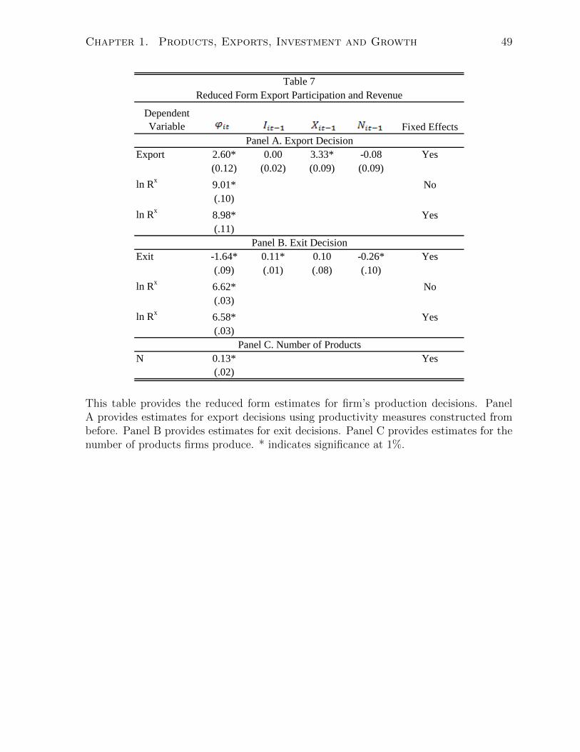
Chapter 1. Products, Exports, Investment and Growth 49
Dependent Variable Fixed Effects
Export 2.60* 0.00 3.33* -0.08 Yes(0.12) (0.02) (0.09) (0.09)
ln Rx 9.01* No(.10)
ln Rx 8.98* Yes(.11)
Exit -1.64* 0.11* 0.10 -0.26* Yes(.09) (.01) (.08) (.10)
ln Rx 6.62* No(.03)
ln Rx 6.58* Yes(.03)
N 0.13* Yes(.02)
Table 7Reduced Form Export Participation and Revenue
Panel A. Export Decision
Panel B. Exit Decision
Panel C. Number of Products
This table provides the reduced form estimates for firm’s production decisions. PanelA provides estimates for export decisions using productivity measures constructed frombefore. Panel B provides estimates for exit decisions. Panel C provides estimates for thenumber of products firms produce. * indicates significance at 1%.

Chapter 1. Products, Exports, Investment and Growth 50
Parameter Mean St. Dev. In EurosEntry sunk cost 19.7 2.25 359 millionDomestic fixed cost 12 0.41 .16 millionProduct fixed cost 11 0.36 59 thousandExport fixed cost 13.5 0.45 .73 millionInvestment Fixed Cost 10.4 0.32 32 thousandd (investment cost) 1 0.01avg sell-off value 16 0.92 8.9 million
Table 8Dynamic Parameter Estimates
This table provides the estimated coefficients for the dynamic parameters in the modeland the correponding dollar values for these estimates.
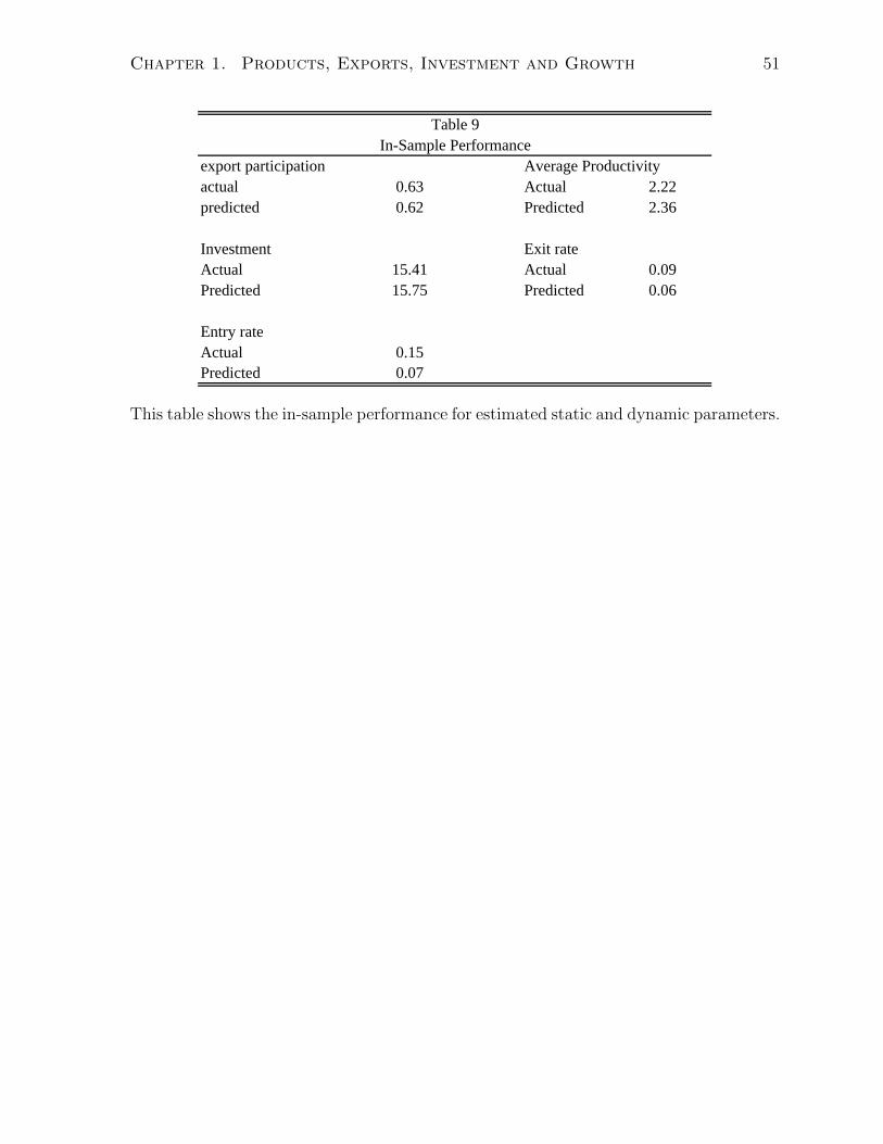
Chapter 1. Products, Exports, Investment and Growth 51
export participation Average Productivityactual 0.63 Actual 2.22predicted 0.62 Predicted 2.36
Investment Exit rateActual 15.41 Actual 0.09Predicted 15.75 Predicted 0.06
Entry rateActual 0.15Predicted 0.07
Table 9In-Sample Performance
This table shows the in-sample performance for estimated static and dynamic parameters.

Chapter 1. Products, Exports, Investment and Growth 52
Tab
le10
Inve
stm
ent
and
Exp
ort
Com
ple
men
tari
ty
prod
ucti
vity
V(X
,I,N
)V
(X,I
=0,
N)
V(X
=0,
I,N
)V
(X=
0,I=
0,N
)M
BE
MB
E
(I=
0)M
BE
-M
BE
(I=
0)1.
916
.44
16.4
416
.44
16.4
40.
000.
000.
002
16.7
316
.48
16.6
616
.48
0.08
0.00
0.08
2.1
16.9
616
.53
16.8
016
.53
0.16
0.00
0.16
2.2
17.2
716
.57
16.9
816
.57
0.29
0.00
0.29
2.3
17.6
516
.66
17.2
116
.66
0.43
0.00
0.43
2.4
18.0
816
.84
17.4
916
.80
0.59
0.04
0.55
2.5
18.5
317
.14
17.7
917
.02
0.74
0.11
0.62
2.6
18.9
817
.55
18.1
117
.32
0.87
0.23
0.64
2.7
19.4
318
.13
18.4
917
.76
0.94
0.37
0.57
2.8
19.7
718
.81
19.0
018
.29
0.77
0.51
0.26
2.9
20.4
019
.53
19.5
718
.87
0.84
0.66
0.18
321
.10
20.3
020
.16
19.5
00.
940.
800.
14
Tab
le 1
2 I
nves
tmen
t and
Exp
ort C
ompl
emen
tari
ty
This
table
show
sth
ein
vest
men
tan
dex
por
tco
mple
men
tari
ty.
All
valu
esar
ein
logs
.M
BE
ism
argi
nal
ben
efit
ofex
por
ting
and
isdefi
ned
asV
(X,I
,N)-
V(X
=0,
I,N
),w
her
eV
(X,I
,N)
isth
eva
lue
funct
ion
when
all
thre
ech
oice
s,X
,I,
and
Nar
ech
osen
opti
mal
lyan
dth
edynam
icpar
amet
ers
are
com
pute
dusi
ng
max
imum
like
lihood
esti
mat
or.
V(X
=0,
I,N
)is
the
valu
efu
nct
ion
when
exp
ort
isre
stri
cted
to0
and
Ian
dN
are
chos
enop
tim
ally
wit
hen
try
and
exit
rate
fixed
asin
V(X
,I,N
).M
BE
(I=
0)is
the
mar
ginal
ben
efit
ofex
por
ting
when
inve
stm
ent
isre
stri
cted
to0
and
isdefi
ned
asV
(X,I
=0,
N)-
V(X
=0,
I=0,
N).
The
cros
spar
tial
bet
wee
nI
and
Xis
defi
ned
asM
BE
-M
BE
(I=
0).
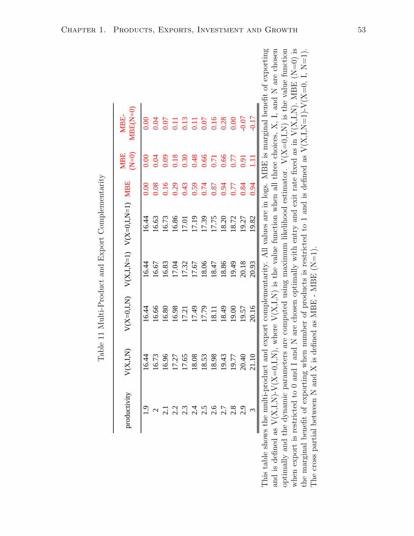
Chapter 1. Products, Exports, Investment and Growth 53
Tab
le11
Mult
i-P
roduct
and
Exp
ort
Com
ple
men
tari
ty
prod
ucti
vity
V(X
,I,N
)V
(X=
0,I,
N)
V(X
,I,N
=1)
V(X
=0,
I,N
=1)
MB
EM
BE
(N
=0)
MB
E-
MB
E(N
=0)
1.9
16.4
416
.44
16.4
416
.44
0.00
0.00
0.00
216
.73
16.6
616
.67
16.6
30.
080.
040.
042.
116
.96
16.8
016
.83
16.7
30.
160.
090.
072.
217
.27
16.9
817
.04
16.8
60.
290.
180.
112.
317
.65
17.2
117
.32
17.0
10.
430.
300.
132.
418
.08
17.4
917
.67
17.1
90.
590.
480.
112.
518
.53
17.7
918
.06
17.3
90.
740.
660.
072.
618
.98
18.1
118
.47
17.7
50.
870.
710.
162.
719
.43
18.4
918
.86
18.2
00.
940.
660.
282.
819
.77
19.0
019
.49
18.7
20.
770.
770.
002.
920
.40
19.5
720
.18
19.2
70.
840.
91-0
.07
321
.10
20.1
620
.93
19.8
20.
941.
11-0
.17
Tab
le 1
3 M
ulti
prod
uct a
nd E
xpor
t Com
plem
enta
rity
This
table
show
sth
em
ult
i-pro
duct
and
exp
ort
com
ple
men
tari
ty.
All
valu
esar
ein
logs
.M
BE
ism
argi
nal
ben
efit
ofex
por
ting
and
isdefi
ned
asV
(X,I
,N)-
V(X
=0,
I,N
),w
her
eV
(X,I
,N)
isth
eva
lue
funct
ion
when
all
thre
ech
oice
s,X
,I,
and
Nar
ech
osen
opti
mal
lyan
dth
edynam
icpar
amet
ers
are
com
pute
dusi
ng
max
imum
like
lihood
esti
mat
or.
V(X
=0,
I,N
)is
the
valu
efu
nct
ion
when
exp
ort
isre
stri
cted
to0
and
Ian
dN
are
chos
enop
tim
ally
wit
hen
try
and
exit
rate
fixed
asin
V(X
,I,N
).M
BE
(N=
0)is
the
mar
ginal
ben
efit
ofex
por
ting
when
num
ber
ofpro
duct
sis
rest
rict
edto
1an
dis
defi
ned
asV
(X,I
,N=
1)-V
(X=
0,I,
N=
1).
The
cros
spar
tial
bet
wee
nN
and
Xis
defi
ned
asM
BE
-M
BE
(N=
1).

Chapter 1. Products, Exports, Investment and Growth 54
Tab
le12
Inve
stm
ent
and
Mult
i-P
roduct
Com
ple
men
tari
ty
prod
ucti
vity
V(X
,I,N
)V
(X,I
=0,
N)
V(X
,I,N
=1)
V(X
,I=
0,N
=1)
MB
IM
BI
(N=
1)M
BI
- M
BI(
N=
1)
1.9
16.4
416
.44
16.4
416
.44
0.00
0.00
0.00
2.0
16.7
316
.48
16.6
716
.48
0.25
0.19
0.06
2.1
16.9
616
.53
16.8
316
.52
0.43
0.30
0.13
2.2
17.2
716
.57
17.0
416
.56
0.70
0.48
0.22
2.3
17.6
516
.66
17.3
216
.64
0.99
0.67
0.31
2.4
18.0
816
.84
17.6
716
.81
1.24
0.86
0.38
2.5
18.5
317
.14
18.0
617
.07
1.39
0.99
0.40
2.6
18.9
817
.55
18.4
717
.48
1.43
0.99
0.44
2.7
19.4
318
.13
18.8
618
.04
1.30
0.82
0.48
2.8
19.7
718
.81
19.4
918
.71
0.97
0.78
0.19
2.9
20.4
019
.53
20.1
819
.44
0.87
0.74
0.13
3.0
21.1
020
.30
20.9
320
.22
0.80
0.72
0.08
Tab
le 1
4 I
nves
tmen
t and
Mul
tipr
oduc
t Com
plem
enta
rity
This
table
show
sth
ein
vest
men
tan
dm
ult
i-pro
duct
com
ple
men
tari
ty.
All
valu
esar
ein
logs
.M
BI
ism
argi
nal
ben
efit
ofin
vest
men
tan
dis
defi
ned
asV
(X,I
,N)-
V(X
,I=
0,N
),w
her
eV
(X,I
,N)
isth
eva
lue
funct
ion
when
all
thre
ech
oice
s,X
,I,
and
Nar
ech
osen
opti
mal
lyan
dth
edynam
icpar
amet
ers
are
com
pute
dusi
ng
max
imum
like
lihood
esti
mat
or.
V(X
,I=
0,N
)is
the
valu
efu
nct
ion
when
inve
stm
ent
isre
stri
cted
to0
and
Xan
dN
are
chos
enop
tim
ally
wit
hen
try
and
exit
rate
fixed
asin
V(X
,I,N
).M
BI
(N=
1)is
the
mar
ginal
ben
efit
ofin
vest
men
tw
hen
num
ber
ofpro
duct
sis
rest
rict
edto
1an
dis
defi
ned
asV
(X,I
,N=
1)-
V(X
,I=
0,N
=1)
.T
he
cros
spar
tial
bet
wee
nI
and
Nis
defi
ned
asM
BI
-M
BI
(N=
1).
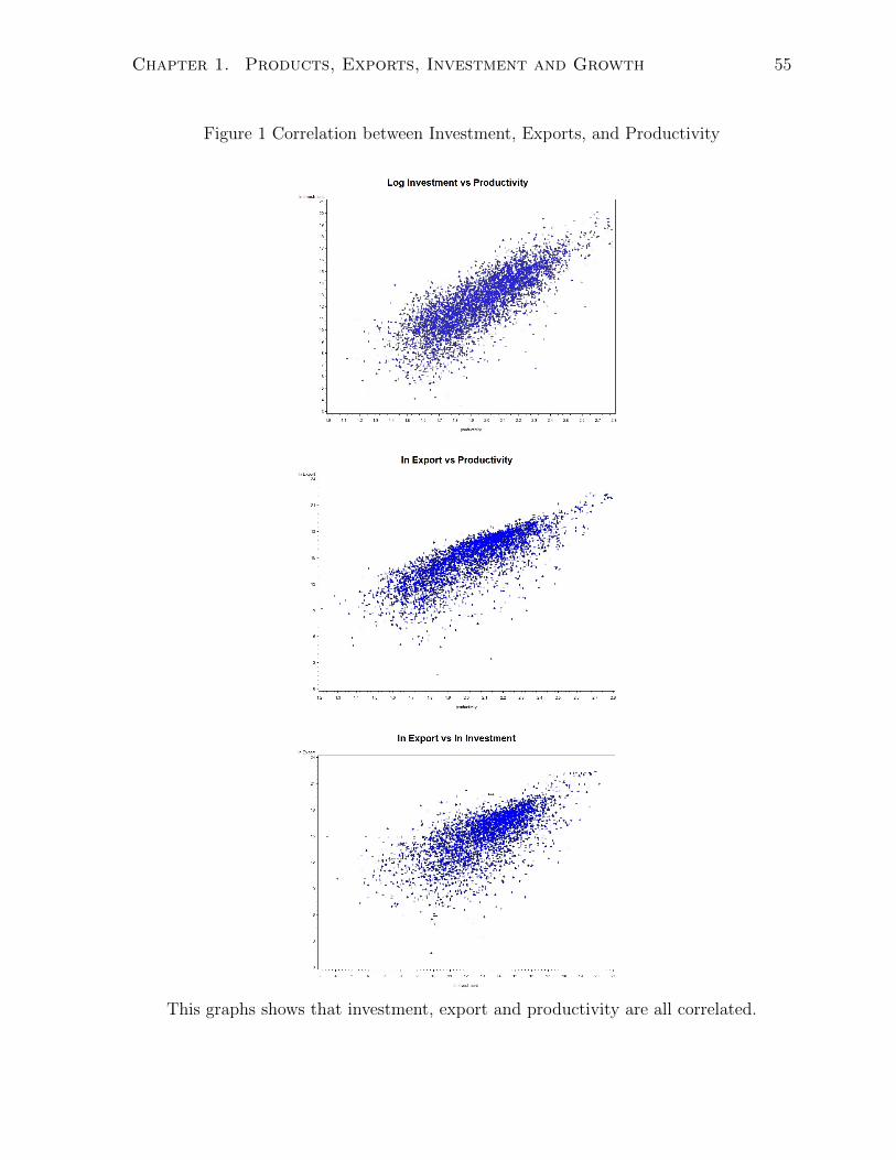
Chapter 1. Products, Exports, Investment and Growth 55
Figure 1 Correlation between Investment, Exports, and Productivity
This graphs shows that investment, export and productivity are all correlated.
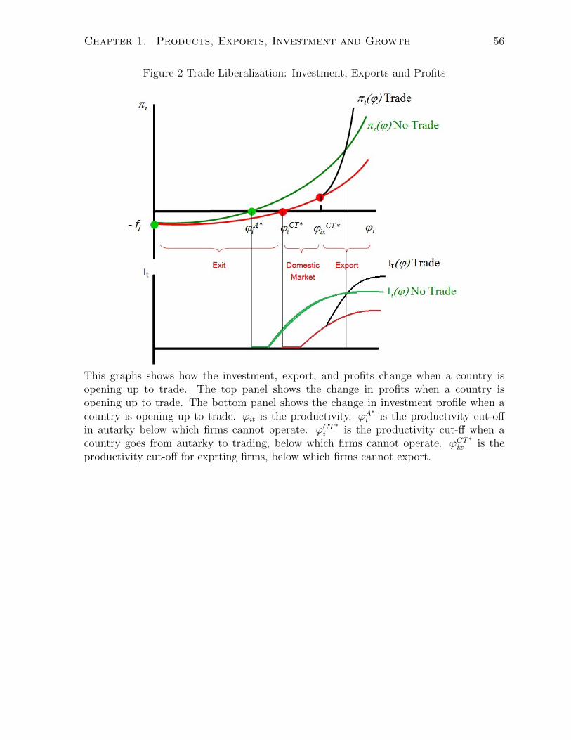
Chapter 1. Products, Exports, Investment and Growth 56
Figure 2 Trade Liberalization: Investment, Exports and Profits
This graphs shows how the investment, export, and profits change when a country isopening up to trade. The top panel shows the change in profits when a country isopening up to trade. The bottom panel shows the change in investment profile when acountry is opening up to trade. ϕit is the productivity. ϕA
∗i is the productivity cut-off
in autarky below which firms cannot operate. ϕCT∗
i is the productivity cut-ff when acountry goes from autarky to trading, below which firms cannot operate. ϕCT
∗ix is the
productivity cut-off for exprting firms, below which firms cannot export.
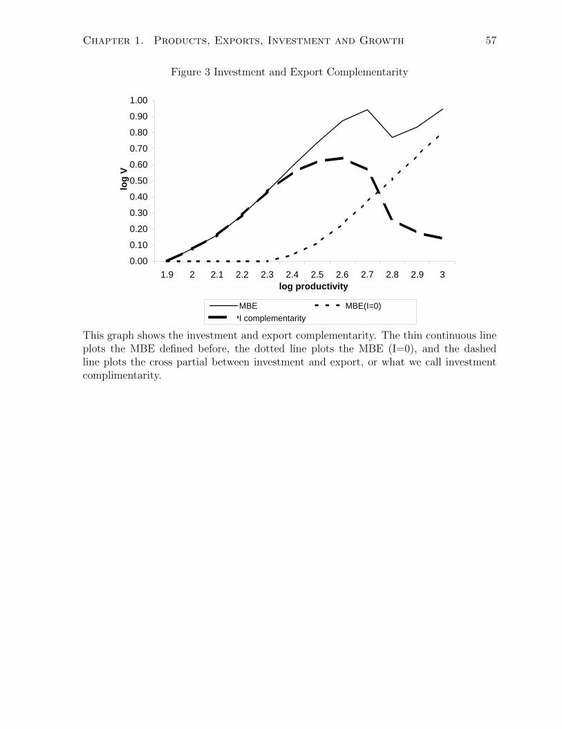
Chapter 1. Products, Exports, Investment and Growth 57
Figure 3 Investment and Export ComplementarityInvestment Complementarity
0.00
0.10
0.20
0.30
0.40
0.50
0.60
0.70
0.80
0.90
1.00
1.9 2 2.1 2.2 2.3 2.4 2.5 2.6 2.7 2.8 2.9 3log productivity
log
V
MBE MBE(I=0)
I complementarity
This graph shows the investment and export complementarity. The thin continuous lineplots the MBE defined before, the dotted line plots the MBE (I=0), and the dashedline plots the cross partial between investment and export, or what we call investmentcomplimentarity.
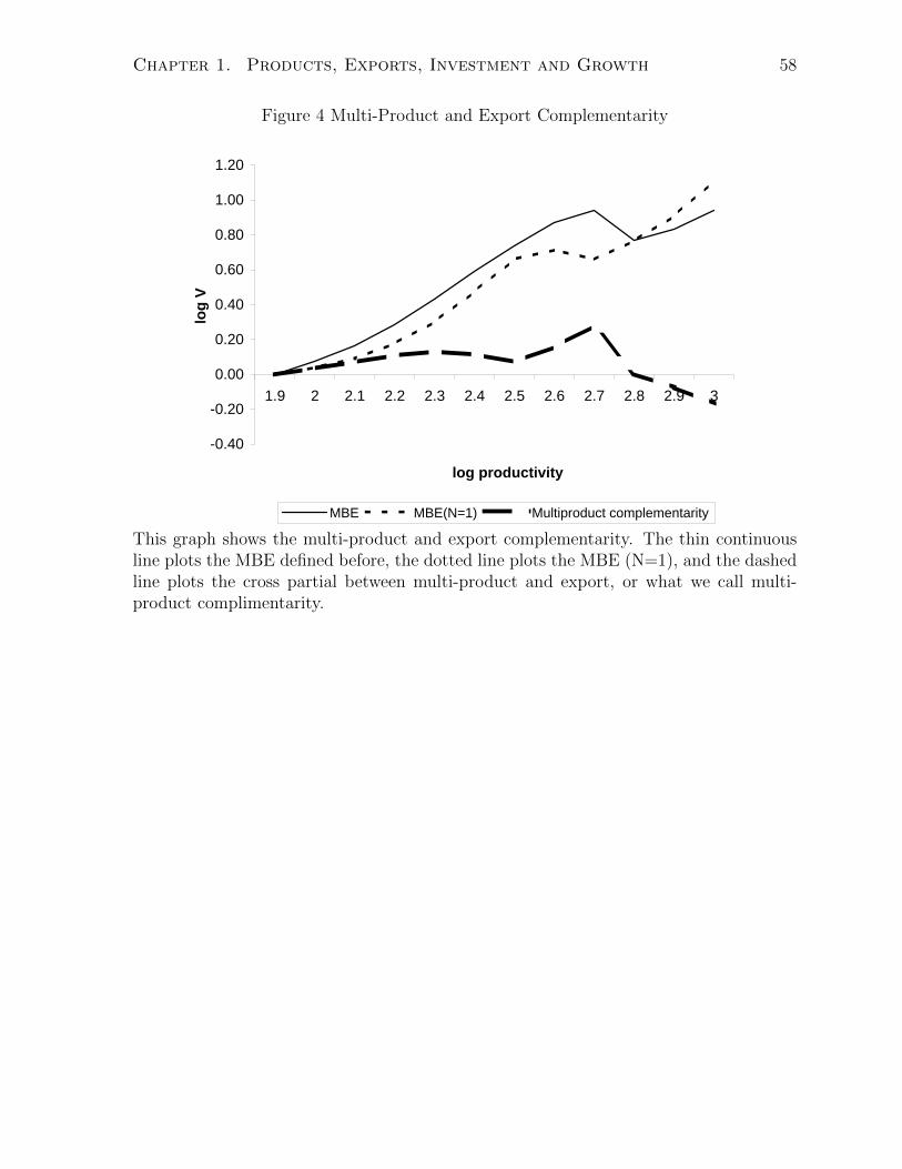
Chapter 1. Products, Exports, Investment and Growth 58
Figure 4 Multi-Product and Export ComplementarityMultiproduct Complementarity
-0.40
-0.20
0.00
0.20
0.40
0.60
0.80
1.00
1.20
1.9 2 2.1 2.2 2.3 2.4 2.5 2.6 2.7 2.8 2.9 3
log productivity
log
V
MBE MBE(N=1) Multiproduct complementarity
This graph shows the multi-product and export complementarity. The thin continuousline plots the MBE defined before, the dotted line plots the MBE (N=1), and the dashedline plots the cross partial between multi-product and export, or what we call multi-product complimentarity.

Chapter 1. Products, Exports, Investment and Growth 59
Figure 5 Investment and Multi-Product ComplementarityMultiproduct and I
0.00
0.20
0.40
0.60
0.80
1.00
1.20
1.40
1.60
1.9 2 2.1 2.2 2.3 2.4 2.5 2.6 2.7 2.8 2.9 3log productivity
log
V
MBI MBI(N=1) Multiproduct complementarity
This graph shows the investment and multi-prodcut complementarity. The thin contin-uous line plots the MBI defined before, the dotted line plots the MBI (N=1), and thedashed line plots the cross partial between investment and multi-product, or what wecall investment-multi-product complimentarity.

Chapter 1. Products, Exports, Investment and Growth 60
Appendix
Capital Size
Capital in the Spanish survey is defined as the value of the technical facilities, machinery,
tools, other facilities, furniture, information processing equipment, rolling stock and other
tangible fixed assets (land and buildings excluded). Capital and Investment have a
correlation coefficient of 0.63.
I break the Spanish data into two subgroups based on capital size in the year 2002. For
simplicity, I’m assuming firms cannot move from the low capital group to the high capital
group within the sample period. For the high capital group, the export participation
rate is 88% and the investment participation rate is 91%. For the low capital group,
the export participation rate is 40% and the investment participation rate is 68%. The
average export and investment volumes for the high capital group are 58 million and 49
million euros, respectively. For the low capital group, they are 350 thousand and 640
thousand, respectively.
I estimate the dynamic parameters for the two subgroups and find that the investment
and export complementarity effect is smaller for the high capital group and the investment
and export complementarity effect is bigger for the low capital group than if I estimate
the whole sample without accounting for capital size. This is because in the high capital
group, most firms already export, the marginal benefit of exporting with zero investment
is higher for these firms with high capital which are also of high productivity. As a result,
the cross partial between investment and export is reduced. Similarly, for the low capital
group, most firms do not export, the marginal benefit of exporting with zero investment
is very low for these firms with low capital which are also of low productivity. As a
result, the difference between the marginal benefit of exporting with optimal investment
and zero investment becomes bigger.
Chapter 1. Products, Exports, Investment and Growth 61
Sample Coverage and Data Collection
The ESEE’s population of reference is made up by the firms with 10 or more employees
and which belong to what is usually known as the manufacturing industry. The geo-
graphical scope of reference is all the Spanish territory, and the variables have a yearly
temporal dimension.
One of the most relevant characteristics of the ESEE is its representativeness. The
initial selection was carried out combining exhaustiveness and random sampling criteria.
In the first category were included those firms which have over 200 employees, and whose
participation was required. The second category was composed by the firms which em-
ploy between 10 and 200 workers, which were selected through a stratified, proportional,
restricted and systematic sampling, with a random start. Each year, all the newly in-
corporated firms which employ over 200 workers, as well as a randomly selected sample
which represents around 5% of the newly incorporated firms which have between 10 and
200 employees enter into the sample.

Chapter 1. Products, Exports, Investment and Growth 62
Computation of the Firm’s Dynamic Problem
Algorithm: MPE solver
1. $ = 0 and $ =1
θEN
(supϕ,s π(ϕ, s)
1− β+ φ
)2. µ(ϕ) = 0 for all ϕ
3. n = 0
4. Loop
5. $ = ($ + $) /2
6. Loop
7. Choose µ∗ to maximize V (ϕ, s|µ,$) for all ϕ
8 ∆ = ||µ∗ − µ||∞ n = n+ 1
9. µ = µ+ (µ∗ − µ)/(nγ +N)
10. until ∆ ≤ ε1
11. if βEµ [V (ϕ, st+1|µ,$)|st = s]− θEN ≥ 0 then
12. $ = $
13. else
14. $ = $
15.until |βEµ [V (ϕ, st+1|µ,$)|st = s]− θEN | ≤ ε2

Chapter 1. Products, Exports, Investment and Growth 63
Table
Su
mm
ary
of
the s
am
ple
’s e
volu
tion
in
th
e y
ears
19
90
-20
08
1
99
1
19
92
1
99
3
19
94
1
99
5
19
96
1
99
7
19
98
1
99
9
20
00
2
00
1
20
02
2
00
3
20
04
2
00
5
20
06
2
00
7
20
08
1. C
urr
en
t sa
mp
le
2188
2059
1977
1869
1876
1703
*
1716
1920
1776
1754
1870
1724
1708
1380
1374
1911
2023
2013
1
.1 F
irm
s w
hic
h
an
swer
1888
1898
1768
1721
1693
1584
1596
1764
1631
1634
1693
1635
1380
1374
1277
1716
1892
1853
1
.2 D
isap
pear1
62
52
72
53
51
28
35
18
45
38
20
18
51
4
17
35
30
57
1
.3 D
o n
ot
collab
ora
te
187
62
124
45
55
33
54
22
35
24
0
12
88
0
12
14
18
10
1
.4 N
o a
ccess
2
51
47
13
50
77
58
31
116
65
58
157
59
189
2
68
146
83
93
2. R
eco
vere
d3
129
99
73
46
0
3
2
3. En
trie
s in
th
e c
urr
en
t year
42
79
101
56
9
132
324
12
123
236
31
0
0
0
588
307
118
154
Nu
mb
er
of
reco
rd o
n f
ile
2359
2438
2539
2595
2604
2736
3060
3072
3195
3431
3462
3462
3462
3462
4050
4357
4475
4629
Not
as:
1.
Clo
sure
s, f
irm
s in
liq
uid
ation,
chan
ge
to a
non-m
anufa
cturing a
ctiv
ity,
dis
appea
rance
thro
ugh m
erger
or
acquis
itio
n.
2.
Can
not
be
found,
pro
visi
onal
clo
se-u
p.
3.
In 1
991 t
hey
are
lar
ge-
size
d f
irm
s to
whic
h t
he
ques
tion
nai
re w
as a
lrea
dy
subm
itte
d in 1
990,
but
whic
h d
id n
ot a
nsw
er it.
In 1
994 it
is m
ade
up o
f la
rge-
size
d firm
s w
hic
h h
ad fill
ed t
he
ques
tion
nai
re b
efor
e but
whic
h a
t so
me
tim
e th
ey s
topped
doi
ng it.
*
Incl
udes
a c
om
pan
y w
hic
h d
id n
ot
colla
bora
ted in 1
995 b
ut
whic
h c
olla
bora
ted in 1
996.
The table shows the evolution of the sampled firms during the period 1990-2007

Chapter 1. Products, Exports, Investment and Growth 64
1
SAMPLE COVERAGE ESEE 2005*
Less than
20 21 to 50 51 to 100 101 to 200 More than
200 Meat-processing industry 1.54% 3.03% 2.04% 14.29% 32.00%Foodstuffs and tobacco 2.42% 3.10% 3.97% 5.32% 38.75%Drinks 3.32% 3.40% 7.41% 23.81% 41.03%Textiles 3.06% 3.75% 6.98% 16.04% 42.62%Leather and footware 3.03% 4.67% 5.63% 14.81% 14.29%Wood industry 1.37% 3.25% 7.69% 16.67% 50.00%Paper 3.53% 3.38% 6.82% 14.29% 60.53%Editing and printing 1.98% 2.96% 6.67% 7.08% 40.32%Chemical industry 2.25% 4.28% 6.61% 11.03% 39.16%Rubber and plastics 3.09% 2.95% 5.79% 12.90% 46.43%Non-metallic minerals products 2.35% 3.34% 2.60% 10.18% 43.40%Iron and steel 2.12% 3.02% 5.65% 14.29% 48.57%Metallic products 2.01% 2.88% 5.31% 7.45% 41.67%Machinery and mechanical goods 2.41% 3.27% 5.42% 12.84% 51.95%Office machinery, computers, processing, optical and similar 1.54% 5.63% 13.64% 4.55% 45.45%Electrical and electronic machinery and material 3.06% 3.95% 4.81% 11.70% 45.83%Motor vehicles 2.74% 3.85% 6.19% 12.66% 44.85%Other transport material 1.57% 6.15% 13.04% 44.00% 31.58%Furniture 2.45% 3.31% 4.86% 12.00% 50.00%Other manufacturing 3.06% 2.73% 2.70% 9.38% 40.00%Total 2.36% 3.37% 5.44% 11.40% 42.95% * Sample coverage, calculated with respect to the Spanish Social Security Census
The table shows the sample coverage.
Chapter 2
Global Sourcing and Credit
Constraints
65

Chapter 2. Global Sourcing and Credit Constraints 66
2.1 Introduction
A growing literature in international economics has emphasized the importance of finan-
cial development in facilitating trade. This literature has addressed questions including
but not limited to how financial development promotes increased exports of finance in-
tensive industries (e.g. Manova (2008) and Manova and Chor (2012)) and the importance
of financial development in providing trade financing (e.g. Amiti and Weinstein (2009)).
Within global supply chains, one of the implications of this literature is that international
supply chain operations necessitate confidence in global suppliers to deliver their share
of valued-added and to have the necessary financial means to produce and export it in a
timely manner.1 This paper examines in detail how differences in financial depth across
countries and credit constraints across industries affect the organization of global supply
chains.
To do so, this paper extends the work of Antras and Helpman (2004) to explain how
the disruption in the ability of the financial sector to provide working capital leads to
a shift in the global supply chain from arm’s length transactions to vertical integration
and contraction in trade. It also shows how the magnitude of this relationship depends
crucially on credit constraints in an industry due to how well industry assets can serve
as collateral. In addition, firms of varying productivity levels within an industry chose
different organizational structures. Finally, the model generates predictions that can be
easily verified in the data. First, it generates classic comparative advantage predictions
regarding country-industry level patterns of specialization depending on country-level
financial depth and industry-level credit constraints. Second, it incorporates firm hetero-
geneity and can therefore analyze how firms of varying productivity levels in an industry
1To meet liquidity needs, firms often obtain trade finance from banks and other financial institutions.These financial arrangements are backed by collateral in the form of tangible assets. Therefore, there is avery active market that operates for the financing and insurance of international transactions, reportedlyworth 10−12 trillion – that is roughly 80% of 2008 trade flows valued at $15 trillion. Up to 90% of worldtrade has been estimated to rely on some form of finance (Auboin (2009)).

Chapter 2. Global Sourcing and Credit Constraints 67
choose different organizational structures and how this sorting depends on financial depth
and credit constraints. Third, it takes patterns of industrial specialization and can ana-
lyze what proportion of trade occurs within the boundary of the firm. While most prior
studies focus on export volumes, I explore the patterns of multinational firm activity.
This allows me to study how credit constraints explain not only export volumes but also
how firms choose to produce intermediate inputs.
More precisely, I develop a multi-sector model of credit-constrained heterogeneous
firms financing their fixed organizational costs, countries at different levels of financial
development, and sectors of varying financial dependence. Production of a final good
requires two inputs, headquarter services, and intermediate inputs. Headquarter ser-
vices are only provided in the North. As in AH, a fixed organizational cost depends
on whether the supplier of intermediate inputs resides in the North or the South and
whether exchange occurs at arm’s length or within the boundary of the firm. I assume
that under vertical integration, the final good producer provides financing for these fixed
costs. While under outsourcing, the intermediate supplier is responsible. Intuitively, in
the case of establishing subsidiaries, parent firms often must incur the upfront fixed costs
that cannot be financed out of retained earnings or internal cash flows from operations.
With independent intermediate input suppliers, the burden lies on the independent in-
termediate input suppliers to finance such costs. Finally, the firm that is responsible for
financing the costs faces the credit constraint of the country in which it is located and
parties choose the organizational structure that maximizes ex-post surplus.
As shown in Rajan and Zingales (1998), financial dependence and credit constraints
vary dramaticaly across both countries and industries. For example, sectors differ in
their endowment of tangible assets that can serve as collateral (Braun (2003)). Final-
good producers in some sectors find it easier to operate because they can more easily
raise outside finance because they possess more tangible assets that can serve as collateral.
Credit constraints vary across countries because financial contracts between firms and

Chapter 2. Global Sourcing and Credit Constraints 68
investors are more likely to be enforced at higher levels of financial development. If
the financial contract is enforced, the financing firm makes a payment to the investor;
otherwise the financing firm defaults and the investor claims the collateral. Financing
firms then find it easier to raise external finance in countries with high levels of financial
contractibility. The need to rely on external finance is common across firms. Firms
often rely on external capital to finance upfront fixed costs, such as investment in fixed
capital equipment, expenditures on R&D and product development, marketing research
and advertising. When production requires the use of intermediate inputs, the final good
producers can choose to open their own subsidiaries or find independent suppliers to
produce them.
In the absence of credit constraints, all final-good producers above a certain cut-off
level operate and sort to different type and location of organizational forms according to
their productivity level. With credit constraints in the South, more Northern firms choose
to integrate with Southern firms relative to arm’s length transactions. This is because the
Northern firms can cover the fixed costs of production using the well developed Northern
financial system more easily than if fixed costs were covered using the Southern financial
system. For similar reasons, integration with other Northern input suppliers (using the
Northern financial system) becomes more attractive relative to arm’s length transactions
with Southern input suppliers.
The empirical section of the paper examines two of the core predictions of the theo-
retical model. First, improvements in financial contractibility in the South increases the
proportion of arm’s length trade between the North and the South. Second, this effect
is most pronounced in the sectors that depend more on external finance and have less
tangible assets. I find strong support for the model’s predictions in a sample of intra-firm
U.S. imports from 90 exporting countries and 429 4-digit SIC manufacturing sectors in
1996-2005. I show how the interaction of country level financial development and in-
dustry level external dependence on finance and asset tangibility predict the choice of

Chapter 2. Global Sourcing and Credit Constraints 69
organizational forms. I use credit extended to the private sector as a share of GDP as my
measure of financial development, and show consistent results with indices of accounting
standards, risk appropriation, contract repudiation, and stock capitalization. I measure
sector-level financial dependence in two ways. First, a sector relies more on external
finance if it possesses a high share of investment not financed from internal cash flows.
Second, asset tangibility for collateral purposes is constructed as the share of structures
and equipment in total assets.
The rest of the paper is organized as follows. Section 2 describes the relation to
the literature. Section 3 provides an overview of trade patterns in the data. Section
4 develops the model. Section 5 shows how firms with different productivity sort into
different organizational forms and the role credit constraint plays on the firms’ sourcing
decisions. Section 6 provides the empirical specification to test. Section 7 discusses the
data. Section 8 provides the regression results. Section 9 concludes.
2.2 Relation to the literature
Prior theoretical and empirical work has focused on the effect of financial development
on industry-level outcomes and on factors that determine the boundary of the firm, but
rarely the two together. A number of studies have proposed that financial development
becomes a source of comparative advantage and affects aggregate growth and volatil-
ity (Rajan and Zingales (1998), Braun (2003),Aghion et al. (2010)). There has been
robust empirical evidence that financially developed countries export relatively more
in financially dependent sectors.2 In addition, there has also been evidence that host
country financial development has implications for patterns of multinational firm activ-
ity and foreign direct investment flows (Antras, Desai, and Foley (2009)). Using Chinese
transaction-level data, Manova, Wei, and Zhang (2011) show that foreign-owned affiliates
2Beck (2002), Beck (2003), Becker and Greenberg (2005), Hur, Raj, and Riyanto (2006), Svalerydand Vlachos (2005), Manova (2006), Manova (2008), Chaney (2005).
Chapter 2. Global Sourcing and Credit Constraints 70
and joint ventures have better export performance than private domestic firms, and that
this advantage is systematically greater in sectors that require more external finance.
Manova (2008) show that financial liberalizations increase exports disproportionately
more in financially dependent sectors that require more outside finance or employ fewer
assets that can be collateralized.
More generally, this paper contributes to a line of research that examines institutional
frictions as a source of comparative advantage in international trade. For example, Nunn
(2007) develops an incomplete-contracts model of relationship specific investments and
finds that countries with better contract enforcement have a comparative advantage in
industries intensive in such investments. Claessens and Laeven (2003) and Levchenko
(2007) also show that property rights protection and the rule of law affect international
trade. Antras and Foley (2011) show that transactions are more likely to occur on cash
in advance or letter of credit terms when the importer is located in a country with weak
contractual enforcement and in a country that is further from the exporter. Whereas these
prior studies on institutions and trade focus on export volume, I explore the impact of
financial institutions on the patterns of multinational firm activity.
2.3 First glance at the data
This section presents basic summary statistics and highlights simple correlations in the
data that motivate the theoretical model and empirical analysis. The data set is assem-
bled by the U.S. Census Bureau captures all U.S. international trade between 1996-2005.
This dataset records the product classification, the value and quantity, the destination
(or source) country, the transport mode, and whether the transaction takes place at
arms length or between related parties. Related-party, or intra-firm, trade are shipments
between U.S. companies and their foreign subsidiaries as well as trade between U.S. sub-

Chapter 2. Global Sourcing and Credit Constraints 71
sidiaries of foreign companies and their affiliates abroad.3 Following Antras (2003), I
take the share of intra-firm U.S. imports to be an indicator for prevalence of vertical
integration.
Table 1 demonstrates substantial variation in the organizational behavior of 90 ex-
porting countries in 429 4-digit SIC manufacturing sectors. In panel A, the average
share of related-party trade across countries and sectors is 22% with standard devia-
tion of .31%, and conditional on positive party-related trade, the mean rises to 36% and
standard deviation is .32%. Across all industries, the U.S. imports from an average of
60 countries with a standard deviation of 30. With party-related trade, this number
drops to 35 countries with a standard deviation of 19. The large number of countries
the U.S. firms are trading with allows us to explore the cross country variation in their
financial development on the organizational structures of multinational firms. Panel B
shows the difference in capital-labor ratio and trade volumes for industries that have zero
related-party trade and positive related-party trade. In Antras (2003) and Antras and
Helpman (2004), those sectors with zero related-party trade are componenent intensive
and those with positive related-party trade are headquarter intensive. Conditional on
positive trade volume, 37% of the exporter-sector cells show no intra-firm trade.4 The
average and trade weighted capital-labor ratios for exporter-sector cells show no signifi-
cant difference between industries with zero and strictly positive intra-firm trade. From
panel C, the average trade volume is higher conditional on strictly positive intra-firm
trade. This is consistent with Antras and Helpman (2004)’s model in which the firms
with positive related-party trade tend to have higher revenues.
The first measure of financial development I use is the ratio of credit from banks and
3For imports, firms are related if they either own, control or hold voting power equivalent to 6 percentof the outstanding voting stock or shares of the other organization (see Section 402(e) of the Tariff Actof 1930).
4The capital-labor ratio for each sector is defined as log of the U.S. capital stock in over the numberof production workers in 1994.

Chapter 2. Global Sourcing and Credit Constraints 72
other financial intermediaries to the private sector as a share of GDP.5 In the panel of
90 countries, private credit over GDP ratio varies significantly across countries and over
time.Table 2 summarizes the cross sectional variation for private credit over GDP ratio.
The countries listed are listed in descending order of the average private credit over GDP
ratio over the years. Excluding the U.S., Switzerland, Hong Kong, and Great Britain are
the top three countries that extend most private credit as a share of GDP. Vietnam and
Denmark experienced greatest change in this measure of financial development over the
years.
Sector-level measures of external dependence on finance and asset tangibility are
constructed based on data for all publicly traded U.S. based companies from Compustat.
A firm’s external dependence on finance is defined as capital expenditures minus cash flow
from operations divided by capital expenditures. A sector’s level’s measure of external
dependence on finance is the median firm’s external dependance on finance in a sector,
as proposed by Rajan and Zingales (1998). Asset tangibility is similarly defined as the
share of net property, plant and equipment in total book-value assets for the median
firm in a given sector. Both measures are constructed as averages for the 1996-2005
period. For comparison reasons, after aggregating these measures to 3-digit SIC industry
classification, they appear very similar to those constructed by Braun (2003). In Table
3 panel B, the mean and standard deviation of external dependence on finance across
all sectors are -1.25 and 2.04, respectively. The mean and standard deviation of asset
tangibility are .74 and .73.6 7
5I obtain this measure from Beck et al. (2000).6The sectors in greatest need for outside capital tend to be intensive in up-front investments, such
as professional and scientific equipment and electrical machinery. Apparel and beverages are the sectorsthat require the least amount of outside capital. Sectors with highest level of asset tangibility arepetroleum refineries, paper and products, iron and steel, and industrial chemicals. Sectors with lowestlevel of asset tangibility are toys, electric machinery, and professional equipments.
7As in Rajan and Zingales (1998), using the U.S. as the reference country is convenient due tothe limited data for many other countries. It’s also reasonable to assume the U.S. measures reflectfirms true demand for external finance and tangible assets because U.S. has the most sophisticated andadvanced financial systems. Using U.S. measure also eliminates the potential bias for an industry’sexternal dependence on finance to endogenously respond to a country’s financial development.

Chapter 2. Global Sourcing and Credit Constraints 73
In addition, sectors in greatest need for outside capital tend to have more affiliated
trade with the U.S; and the opposite is true for sectors with greatest assets. Figure 1
shows shares of related-party (intra-firm) trade is computed by aggregating the data to
3-digit SIC classification. It is clear that industries that are more dependent on external
finance are associated with a greater share of U.S. intra-firm trade. Figure 2 illustrates
the opposite relationship for asset tangibility and share of U.S. intra-firm trade. This
relationship persists for all years.
The Asian financial crisis of 1997-1999 provides additional motivation. During an
episode of diminished financial depth, I expect an increase in the share of intra-firm
trade and that this effect is more pronounced in sectors with the most binding credit
constraints. Financial frictions rose during this period as international investors were
reluctant to lend to developing countries. In Figure 3, for each country c and year t,
I calculate the average external finance dependence and asset tangibility for the share
of intra-firm trade as∑
i(FinDepi ∗ Rict/Tict) and∑
i(Tangi ∗ Rict/Tict) respectively,
where Rict/Tict is the share of intra-firm trade in sector i in country c in year t. I plot
both measures for the 12 countries with the largest growth in the credit extended to
private sector as a share of GDP between 1996 and 2004. I expect the average external
finance dependence measure to be higher during financial crunches because the share
of intra-firm trade will be higher, and this is especially true in the sectors that require
greater outside finance. I expect the average asset tangbility measure to be lower during
financial crunches because for sectors that have the greatest tangible assets for collateral,
the share of intra-firm trade will be small. From Figure 3, I see that the average external
finance dependence weighted by the share of intra-firm trade increased in 1997 for most
countries. After year 1999, these values decreased. The opposite is true using the average
asset tangibility weighted by the share of intra-firm trade, because the more tangible
assets firms have, the less financially dependent they are. I also see another spike in
2001, this is likely due to the events of 9-11 and the bursting of the technology bubble,

Chapter 2. Global Sourcing and Credit Constraints 74
where credit tightened around the world and firms became more financially dependent.
The 12 graphs are ordered by the standard deviation of the change in private credit to
GDP ratio over this period as indicated in the graph headings.
The variation in the share of intra-firm trade in the data across countries, sectors
and time are not random. I proceed with the following model to better understand the
mechanisms behind these features.
2.4 The Model
Consider a world consisting of two countries: North (N) and South (S). There are J + 1
sectors consisting of J CES aggregates described below and a single homogenous goods
sector. As described below, firms decide whether to produce, from where to source
intermediate inputs, and the boundaries of the firm.
This section starts by describing consumer preferences and the production technology
of firms. It then describes the incomplete contracting setting and credit constraints that
are at the core of the model. I then derive the profit functions under arm’s length and
integrated sourcing with both Northern and Southern suppliers of intermediate inputs.
Finally, I derive the equilibrium choice of firm boundaries and location of intermediate
input suppliers as a function of credit constraints, financial depth, and firm productivity.
2.4.1 Demand
The utility function of a representative consumer is given by:
U = x0 +1
µ
J∑j=1
Xµj , 0 < µ < 1 (2.1)
Xj =
[∫xj(i)
αdi
]1/α
, 0 < α < 1 (2.2)

Chapter 2. Global Sourcing and Credit Constraints 75
where x0 is the consumption of a homogeneous good, and Xj is the CES aggregate
consumption index in sector j. Each firm produces an imperfectly substitutable variety
xj(i) such that i indexes both firms and varieties. The constant elasticity of substitution
in a sector is given by ε = 1/(1−α) > 1. Assume α > µ, so that varieties within a sector
are more substitutable within than across. Inverse demand for variety i in sector j is:
pj(i) = Xµ−αj xj(i)
α−1 (2.3)
and the revenue function for a given firm is
Rj(i) = Xµ−αj xj(i)
α. (2.4)
2.4.2 Production
The only factor of production is labor. Producers face a perfectly elastic supply of labor
in each country. I assume that the wage rate is fixed in the North and the South and
wN > wS.8 As in Antras and Helpman (2004), only the North produces the final-good
variety. The production of the final good requires two inputs, headquarter services hj(i),
and intermediate inputs, mj(i) using a Cobb-Douglas production function,
xj(i) = θ
[hj(i)
ηj
]ηj [mj(i)
1− ηj
]1−ηj, 0 < ηj < 1 (2.5)
where θ is the productivity of final good producer H of variety i in sector j. θ is drawn
from a known distribution G(θ) after H pays a fixed cost of entry wNfE. ηj is sector
specific, with higher ηj indicating greater intensity of headquarter services. Headquarter
services must be produced in the North, whereas intermediate inputs can be produced in
8The assumption of a higher wage in the North can be justified by assuming that labor supply islarge enough in each country so that both countries produce x0 and that x0 is produced with constantreturns to scale, but with higher productivity in the North.

Chapter 2. Global Sourcing and Credit Constraints 76
either the North or the South. H makes two decisions: whether to source intermediate
inputs in the North or in the South, and whether to vertically integrate the supplier (V )
or to outsource (O). The first is the location decision (l ∈ N,S) and the second is the
organizational-structure decision (k ∈ V,O). Following Antras and Helpman (2004),
the fixed organizational costs are assumed to be ranked in the following order:
fSV > fSO > fNV > fNO . (2.6)
That is, in either location, the costs of vertical integration are higher than the costs of
outsourcing and, for either ownership structure, costs are higher in the South than in the
North.
2.4.3 Credit Constraints
Final good producers and intermediate suppliers face credit constraints in the financing of
fixed costs associated with organizational choice depending on both reliance on external
finance and the tangibility of assets that can serve as collateral. Following Manova (2006),
I begin by assuming all firms can finance their variable costs internally, but they need
to raise outside capital to finance for a fraction dj of the fixed organizational costs.9
Consequently, production requires that H or the M borrow djwNf lk. Firms experience
liquidity constraints because of up-front costs which they can cover after revenues are
realized but not internally in advance. As argues by Rajan and Zingales (1998) I assume
that the reliance on external finance dj varies across industries.10
To obtain external finance, firms must use tangible assets as collateral.11 If the firm
fails to pay back its loan, the creditor receives ownership of the collateral. tj corresponds
90 < dj < 1.10BRIEFLY SUMMARIZE THIS ARGUMENT.11Examples of tangible assets include structures and equipment whereas an example of an intangible
asset is human capital.

Chapter 2. Global Sourcing and Credit Constraints 77
to the measure of asset tangibility in my empirical analysis and is also innate to each
industry, as in Braun (2003). A fraction tj of the sunk costs must be provided as collateral
to obtain external finance such that the total collateral that must be posted is tjwNfE.12
The North and the South varies in their level of financial contractibility. Investors
can be expected to be repaid with probability λl.13 I assume that λN > λS. A final
goods producer located in the North defaults with probability (1−λN), and intermediate
supplier who is located in the North or South defaults with probability (1− λl), and the
investors claim tjwNfE. λ
l is exogenous in the model and corresponds to the strength of
country l’s financial institutions in my empirical analysis.
2.4.4 Incomplete Contracts
As in Antras (2003), final good producers and intermediate input suppliers cannot sign
ex ante enforceable contracts specifying the purchase of specialized intermediate inputs
for a certain price nor a contract contingent on the amount of labor hired or the volume
of sales after the final good is sold.14 Therefore, surplus is split between the final goods
producer and intermediate supplier in generalized Nash bargaining such that the final
good sproducer obtains a fraction β ∈ (0, 1) of the ex post gains from the relationship.
Ex post bargaining takes place both under vertical integration and outsourcing. Under
outsourcing, the outside option of both parties is assumed to be zero because the inputs
are relationship specific and have no outside value. Under vertical integration, failure
to reach an agreement on the distribution of surplus leaves M with no outside value;
however, H can appropriate a fraction δl of the intermediate inputs produced because H
cannot use the intermediate inputs as effectively in an outside relationship as it can with
M .15 I assume δN ≥ δS, as in Antras and Helpman (2004), because a contractual breach
120 < tj < 1130 < λl < 1.14This can be justified as in Hart and Moore (1999) where the precise nature of the intermediate
input is revealed ex post only and is not verifiable by a third party.150 < δl < 1 and δl 6= 1 because if H were able to appropriate all intermediate inputs, H would

Chapter 2. Global Sourcing and Credit Constraints 78
is more costly to H when M is located in the South. This also reflects more corruption
and lack legal protection in the South.
There is infinitely elastic supply of M in each country. Because of this M ’s profits
from the relationship are equal to its outside option, which is assumed to be 0 here.
Consequently, to ensure the relationship is at minimum costs to H, M pays a fee T for
that makes its participation constraint binding.
2.4.5 Equilibrium
Ex-Post Revenue Shares
Looking at a particular sector j and dropping the industry subscript, if H and M agree
in the bargaining, revenue from the sale of the final good is:
R(i) = Xµ−αθα[h(i)
η
]αη [m(i)
1− η
]α(1−η)
. (2.7)
If they fail to agree, the outside option for M is always zero. The outside option for H
varies with ownership structure and the location of M .
When H outsources the intermediate inputs, its outside option is zero. Consequently,
each party obtains a share of ex-post gains from trade R(i) corresponding to their Nash
bargaining weight. Therefore, H obtains βR(i) and M receives (1− β)R(i).
With vertical integration, if Nash bargaining breaks down, H can sell δlx(i) of out-
put when M is in country l, which yields revenue (δl)αR(i). In the bargaining, H
receives its outside option plus a fraction β of the ex post gains from the relation-
ship. Consequently,H receives[(δl)α + β(1− (δl)α)
]R(i) and M receives (1− β) (1 −
(δl)α)R(i).
Using this information, I can order the shares of revenue that accrue to H under the
always have an incentive to seize all inputs, and this would lead M to choose mj(i) = 0 which leavesxj(i) = 0.

Chapter 2. Global Sourcing and Credit Constraints 79
four organizational forms. Let βlkR(i) denotes the payoff of H under ownership structure
k and the location of M in country l, then:
βNV = (δN)α + β(1− (δN)α) ≥ βSV = (δS)α + β(1− (δS)α) > βNO = βSO = β (2.8)
As in Grossman and Hart (1986), integration gives H the right to ex post use the inputs
produced by M , which in turn enhances H’s bargaining position (βlV > βlO).
Ex-Ante Investments and Financing
Since final good producers and intermediate input suppliers cannot sign ex ante enforce-
able contracts, the parties choose their quantities non-cooperatively. In absence of credit
constraint, H provides an amount of headquarter services that maximizes βlkR(i)−wNh(i)
subject and M provides the intermediate input that maximizes (1 − βlk)R(i) − wlm(i)
each subject to (7). Combining the two first-order conditions, the total operating profit
is
πlk(θ,X, η) = X(µ−a)/(1−α)θa/(1−α)ψlk(η)− wNf lk (2.9)
where ψlk(η) =1−α[βlkη+(1−βlk)(1−η)]
(1/α)(wN/βlk)η[wl/(1−βlk)]
1−ηα/(1−α) .Under credit constraints, two additional conditions must be satisfied.
Vertical Integration
If H chooses vertical integration, no matter where the supplier is located, H faces the
financial friction in the North and chooses an amount of headquarter services that max-
imizes
maxh,F (a)
βlVR(i)− wNh(i)− (1− d)wNf lV − λNF (i)− (1− λN)twNfE + T (2.10)

Chapter 2. Global Sourcing and Credit Constraints 80
subject to (1) R(i) = Xµ−αθα[h(i)η
]αη [m(i)1−η
]α(1−η)
(2) A(i) ≡ βlVR(i)− wNh(i)− (1− d)wNf lV + T ≥ F (i)
(3) B(i) ≡ −dwNf lV + λNF (i) + (1− λN)twNfE ≥ 0.
I describe each expression in turn. H maximizes its profits by financing all its variable
costs and a fraction (1− d) of its fixed costs internally. With probability λl the contract
is enforced and the investor receives F (i). With probability 1 − λl there is default and
the investor receives the collateral twNfE. T is the ex-ante transfer payment M has to
pay to H that makes M ’s participation constraint binding such that
T = (1− βlV )R(i)− wlm(i). (2.11)
Consider next the financial constraint (2). When financial contract is enforced, H can
offer at most A(i), its net revenue, to the investor. Thus the firm cannot borrow more than
A(i) such that A(i) ≥ F (i). Finally, consider the participation constraint (3). Investors
only lend to H if they expect to at least break even. B(i) represents the expected return to
the investor taking into account the possibility default. With competitive credit markets,
investors break even, H adjusts F (i) to bring investors’ net return to 0, and B(i) = 0.
Therefore, F (i) =dwNf lV −(1−λN )twNfE
λN.
Using equation (11) and the expression for F (i), profits for H under vertical integra-
tion are
maxm
πlHV = R(i)−wNh(i)−wlm(i)− (1− d+d
λN)wNf lV +
(1− λN)
λNtwNfE (2.12)
subject to R(i) = Xµ−αθα[h(i)η
]αη [m(i)1−η
]α(1−η)
.
The profit function for H then becomes
πlHV = X(µ−a)/(1−α)θa/(1−α)ψlV (η)− (1− d+d
λN)wNf lV +
(1− λN)
λNtwNfE.
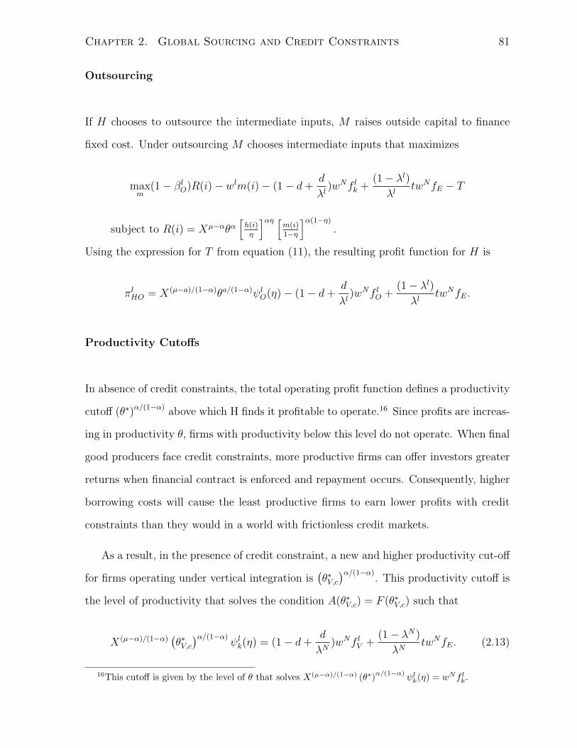
Chapter 2. Global Sourcing and Credit Constraints 81
Outsourcing
If H chooses to outsource the intermediate inputs, M raises outside capital to finance
fixed cost. Under outsourcing M chooses intermediate inputs that maximizes
maxm
(1− βlO)R(i)− wlm(i)− (1− d+d
λl)wNf lk +
(1− λl)λl
twNfE − T
subject to R(i) = Xµ−αθα[h(i)η
]αη [m(i)1−η
]α(1−η)
.
Using the expression for T from equation (11), the resulting profit function for H is
πlHO = X(µ−a)/(1−α)θa/(1−α)ψlO(η)− (1− d+d
λl)wNf lO +
(1− λl)λl
twNfE.
Productivity Cutoffs
In absence of credit constraints, the total operating profit function defines a productivity
cutoff (θ∗)α/(1−α) above which H finds it profitable to operate.16 Since profits are increas-
ing in productivity θ, firms with productivity below this level do not operate. When final
good producers face credit constraints, more productive firms can offer investors greater
returns when financial contract is enforced and repayment occurs. Consequently, higher
borrowing costs will cause the least productive firms to earn lower profits with credit
constraints than they would in a world with frictionless credit markets.
As a result, in the presence of credit constraint, a new and higher productivity cut-off
for firms operating under vertical integration is(θ∗V,c)α/(1−α)
. This productivity cutoff is
the level of productivity that solves the condition A(θ∗V,c) = F (θ∗V,c) such that
X(µ−α)/(1−α)(θ∗V,c)α/(1−α)
ψlk(η) = (1− d+d
λN)wNf lV +
(1− λN)
λNtwNfE. (2.13)
16This cutoff is given by the level of θ that solves X(µ−α)/(1−α) (θ∗)α/(1−α)
ψlk(η) = wNf lk.

Chapter 2. Global Sourcing and Credit Constraints 82
The productivity cut-off for firms operating under outsourcing is
X(µ−α)/(1−α)(θ∗O,c)α/(1−α)
ψlk(η) = (1− d+d
λl)wNf lO +
(1− λl)λl
twNfE. (2.14)
Regardless of organizational structure, there is a higher productivity cut-off under credit
constraint than without. This can be seen by noting that the right hand side of each of
the expressions is increasing as λ falls. Consequently, with lower financial development,
there are higher productivity cutoffs. Without financial frictions (λl = 1), the model
reduces to original Antras and Helpman (2004) formulation. In addition, note that
reliance on external funding (dj) only has an impact when financial contracts are not
perfectly enforced.
Also, note that the payment to investors F (i) is decreasing in financial development.
As financial development falls (λ ↓), intermediate suppliers in the South face a higher
interest rates on loans. This then reduces the transfer payment T ) they can make to
H, and thus H that choose to outsource in the South in essence need to pay a higher
repayment on loans.
Regardless of ownership, Final good producers cannot operate with productivity lower
than min(θ∗V,c, θ∗O,c) when they face credit constraints. min(θ∗V,c, θ
∗O,c) > θ∗ whenever
df lk > tfE, which means credit constraints bind when firms need to borrow more than they
can offer in collateral.17. Consequently, I make the following assumption on the magnitude
of fixed costs to ensure that all four organizational forms can exist in equilibrium:
Assumption 1 dfSO > tfE. Since dfSO is the smallest, df lk > tfE.
I assume this condition holds for the rest of the analysis. In addition, notice that
θ∗V,c > θ∗O,c because f lV > f lO. Figure 4 illustrates the productivity cut-offs between credit
constrained and unconstrained final good producers.
17(Manova (2006), Greenaway et al. (2005), Becker and Greenberg (2005), Beck (2002), and Beck(2003)

Chapter 2. Global Sourcing and Credit Constraints 83
To summarize, after observing its productivity level θ, a final good producerH chooses
the ownership structure and the location of M that maximizes πlHk, or exits the industry
and forfeits the fixed cost of entry wNfE. πlHk(θ,X, η) is decreasing in wlk and f lk. Looking
at variable costs, producing intermediate inputs in the South is preferred to producing
intermediates in the North regardless of ownership structure because wS < wN . Looking
at fixed costs, fSV > fSO > fNV > fNO , ranking of profits is the reverse order of the fixed
costs.
As shown in Antras and Helpman (2004), if final good producer H could freely choose
β,∂βlk∂η
> 0. This means the more intensive a sector is in headquarter services, the higher
βlk H would prefer. Following Grossman and Hart (1986), β cannot be chosen freely, so
the choice of βlk is constrained to the set βNV , βSV , βNO , βSO.
2.5 Organizational Forms
2.5.1 Headquarter Intensive Sector
First consider a sector with high headquarter intensity η, such that profits are increasing
in βlk. In a headquarter intensive sector, the marginal product of headquarter services is
high, making underinvestment in headquarter services more costly and integration more
attractive. Because ψlV > ψlO, πlV is steeper than πlO such that the slope of the profit
function for vertical integration is greater than the slope for outsourcing within a coun-
try. However, the slope of πSO can be steeper than the slope of πNV when the variable
costs in the South are very low, or flatter than the slope of πNV because integration gives
higher the final good producer a larger fraction of the revenue. Figure 5 reflects the
benchmark case when slope of πSO is steeper than the slope of πNV . Unlike the case of the
component intensive sector, all four forms of organization are now possible. The produc-
tivity cut-offs with credit constraints (θ∗c , θNV,c, θ
SO,c, θ
SV,c) and without credit constraints

Chapter 2. Global Sourcing and Credit Constraints 84
(θ∗, θNV , θSO, θ
SV ) are provided in the Appendix.18 Proposition 1 describes how changes in
financial development affect productivity cut-offs under credit constraints.
Proposition 1 For headquarter intensive sectors, firms tend to choose outsourcing in
more financially developed country (∂θSV,c∂λS
> 0,∂θSO,c∂λS
< 0 and∂θSV,c∂λN
< 0,∂θSO,c∂λN
> 0). This
effect is more pronounced in financially dependent sectors (∂θSV,c∂d∂λS
> 0,∂θSO,c∂d∂λS
< 0,∂θSV,c∂t∂λS
<
0,∂θSO,c∂t∂λS
> 0 and∂θSV,c∂d∂λN
< 0,∂θSO,c∂d∂λN
> 0,∂θSV,c∂t∂λN
> 0,∂θSO,c∂t∂λN
< 0). In sectors with higher
headquarter intensity, integration is favored relative to outsourcing ( ∂∂η
ψlV (η)
ψlO(η)> 0 for
l = N,S).
For an improvement in the financial development in the South (λS ↑), the most
productive firms that were vertically integrated in the North now outsource in the South.
The least productive firms firms that integrated in the South now switch to arm’s length
transactions with suppliers in the South. Overall, the proportion of firms conducting
sourcing with suppliers in the South relative to the North increases and revenue of firms
that were both initially and currently sourcing from the South increase. In addition, the
share of vertically integrated firms in the South relative to total firms firms sourcing from
the south will decrease, as depicted in Figure 6. This effect is strongest in sectors that
require more outside capital or possess fewer tangible assets.
For an increase in financial development in the North (λN ↑), the most productive
firms that initially chose to exit now outsource in the North. The most productive firms
that previously outsourced in the North will now vertically integrate and realize higher
revenues. Firms that previously operated in the North continue to operate in the North
and realize higher revenue. Increased financial development in the North lead to fewer
firms conducting sourcing with suppliers in the South through two channels. First, the
least productive firms that were outousrcing in the South now vertically integrate in
the North. Second, the most productive firms that were outsourcing in the South now
18Figure 5 plots the productivity cut-offs without credit constraints. With credit constraints, pro-ductivity cut-offs are increased.

Chapter 2. Global Sourcing and Credit Constraints 85
vertically integrate in the South to take advantage of the improved financial depth in the
North. Overall, increase in financial development in the North leads to higher share of
vertically integrated firms in the South relative to total firms sourcing from the South.
The share of firms and trade that occur via vertical integration relative to at arm’s
length (regardless of location), is increasing in the headquarters intensity of the industry
(ηj). This result is also found in Antras (2003). Notice that any of the first three
organizational forms (outsourcing in North, vertical integration in North, and outsourcing
in South) may not exist in equilibrium but vertical integration with Southern suppliers
always exists due to the absence of an upper bound on support of G(θ). See Figure 6 for
illustration. Organizational forms that survive in equilibrium have firms sorted according
to the order in Figure 6 depending on their productivities.
2.5.2 Component Intensive Sector
Next, consider a sector with sufficiently low headquarter intensity η that H prefers out-
sourcing to integration in every country l. This is because outsourcing has lower fixed
costs and H prefers βlk to be as low as possible, or βlk = βlO = β. H trades off between lower
variable cost in the South against the lower organizational costs in the North. If wage
differential is small relative to the fixed cost differential, wN/wS < (fSO/fNO )(1−α)/α(1−η),
The top panel in Figure 7 depicts the choice of location of M depending on produc-
tivity level θ without credit constraints. As in Antras and Helpman (2004), the cutoffs
θ∗ and θSO are given by:
θ∗ = X(α−κ)/α
[wNfNOψNO (η)
](1−α)/α
,
θSO = X(α−κ)/α
[wN(fNO − fNO )
ψSO(η)− ψNO (η)
](1−α)/α
.
As is clear from Figure 7, firms do not operate with productivity lower than θ∗ and can
only outsource in the South if their productivity level is above θSO. The bottom panel in

Chapter 2. Global Sourcing and Credit Constraints 86
Figure 7 provides analogous cutoffs when there are credit constraints
θ∗c = X(α−κ)/α
[(1− d+ d/λN)wNfNO − 1−λN
λNtwNfE
ψNO (η)
](1−α)/α
,
θSO,c = X(α−κ)/α
(1− d+ d/λS)wNfSO − 1−λSλS
twNfE −[(1− d+ d/λN)wNfNO − 1−λN
λNtwNfE
]ψSO(η)− ψNO (η)
(1−α)/α
.
H firms with productivity lower θ∗c do operate. H outsources in the North when its
productivity is between θ∗c and θSO,c, and outsource in the South when its productivity is
above θSO,c. Proposition 2 provides comparative statics on these cut-offs.
Proposition 2 In component intensive sectors, firms do not integrate. An increase in
financial development in the South leads to more outsourcing in the South (∂θSO,c∂λS
< 0 and
∂θ∗c∂λS
= 0). An increase in financial development in the North leads to less outsourcing
in the South (∂θSO,c∂λN
> 0 and ∂θ∗c∂λN
< 0). This effect is stronger in the sectors that require
more outside capital (∂θSO,c∂d∂λS
< 0 and ∂θ∗c∂d∂λS
= 0 for the South,∂θSO,c∂d∂λN
> 0 and ∂θ∗c∂d∂λN
< 0
for the North ) and less tangible assets (∂θSO,c∂t∂λS
> 0 and ∂θ∗c∂d∂λS
= 0 for the South,∂θSO,c∂t∂λN
< 0
and ∂θ∗c∂t∂λN
> 0 for the North).
An increase in financial development in the South (λS ↑) leads to a lower cut-off
productivity θSO,c for outsourcing firms in the South as depicted in figure 8. The most
productive firms initially outsourcing in the North now switch to outsourcing in the
South to take the advantage of better financial institutions in the South. The profits
of the firms already outsourcing in the South also increase. This is because with less
financial frictions, a smaller repayment is required when the financial contract is enforced.
This effect is stronger for sectors that require more outside capital (d higher) or possess
fewer tangible assets (t lower) as firms in those sectors find it cheaper to outsource from
suppliers located in the South with a more developed financial system.
An increase in the financial development in the North (λN ↑) leads to a lower cut-off
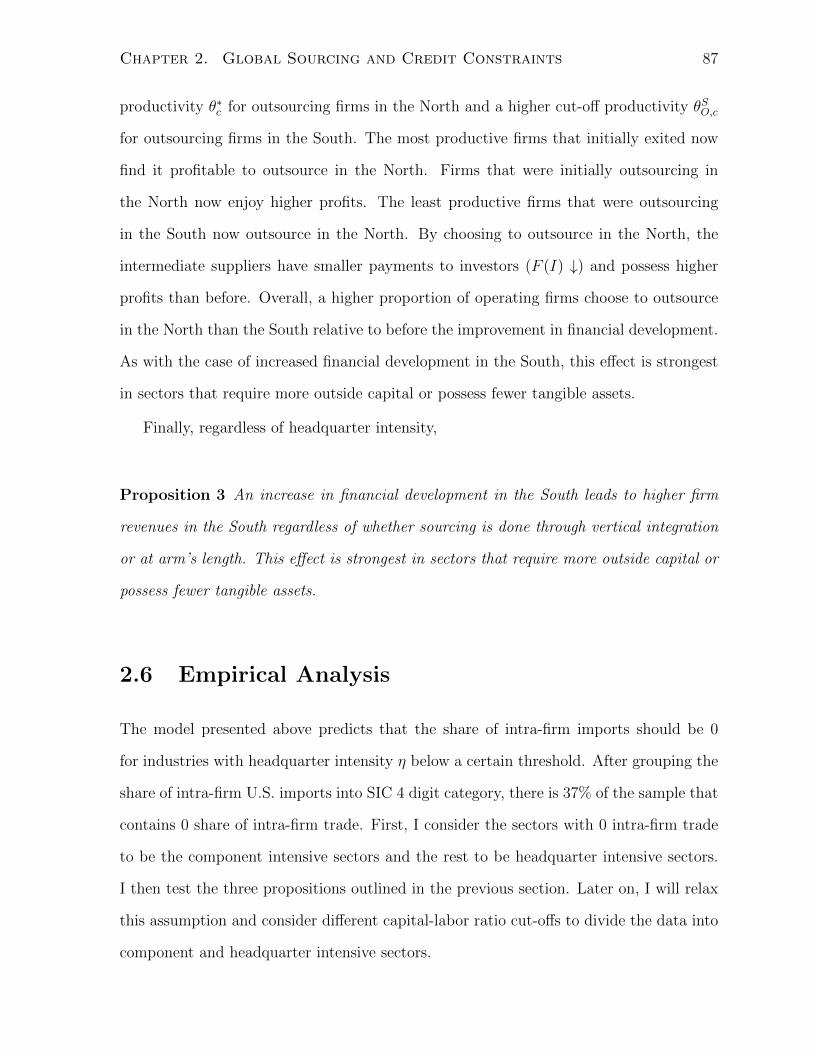
Chapter 2. Global Sourcing and Credit Constraints 87
productivity θ∗c for outsourcing firms in the North and a higher cut-off productivity θSO,c
for outsourcing firms in the South. The most productive firms that initially exited now
find it profitable to outsource in the North. Firms that were initially outsourcing in
the North now enjoy higher profits. The least productive firms that were outsourcing
in the South now outsource in the North. By choosing to outsource in the North, the
intermediate suppliers have smaller payments to investors (F (I) ↓) and possess higher
profits than before. Overall, a higher proportion of operating firms choose to outsource
in the North than the South relative to before the improvement in financial development.
As with the case of increased financial development in the South, this effect is strongest
in sectors that require more outside capital or possess fewer tangible assets.
Finally, regardless of headquarter intensity,
Proposition 3 An increase in financial development in the South leads to higher firm
revenues in the South regardless of whether sourcing is done through vertical integration
or at arm’s length. This effect is strongest in sectors that require more outside capital or
possess fewer tangible assets.
2.6 Empirical Analysis
The model presented above predicts that the share of intra-firm imports should be 0
for industries with headquarter intensity η below a certain threshold. After grouping the
share of intra-firm U.S. imports into SIC 4 digit category, there is 37% of the sample that
contains 0 share of intra-firm trade. First, I consider the sectors with 0 intra-firm trade
to be the component intensive sectors and the rest to be headquarter intensive sectors.
I then test the three propositions outlined in the previous section. Later on, I will relax
this assumption and consider different capital-labor ratio cut-offs to divide the data into
component and headquarter intensive sectors.
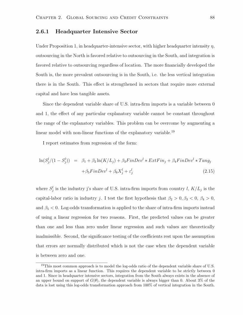
Chapter 2. Global Sourcing and Credit Constraints 88
2.6.1 Headquarter Intensive Sector
Under Proposition 1, in headquarter-intensive sector, with higher headquarter intensity η,
outsourcing in the North is favored relative to outsourcing in the South, and integration is
favored relative to outsourcing regardless of location. The more financially developed the
South is, the more prevalent outsourcing is in the South, i.e. the less vertical integration
there is in the South. This effect is strengthened in sectors that require more external
capital and have less tangible assets.
Since the dependent variable share of U.S. intra-firm imports is a variable between 0
and 1, the effect of any particular explanatory variable cannot be constant throughout
the range of the explanatory variables. This problem can be overcome by augmenting a
linear model with non-linear functions of the explanatory variable.19
I report estimates from regression of the form:
ln(Slj/(1− Slj)) = β1 + β2 ln(K/Lj) + β3FinDevl ∗ ExtF inj + β4FinDev
l ∗ Tangj
+β5FinDevl + β6X
lj + εlj (2.15)
where Slj is the industry j’s share of U.S. intra-firm imports from country l, K/Lj is the
capital-labor ratio in industry j. I test the first hypothesis that β2 > 0, β3 < 0, β4 > 0,
and β5 < 0. Log-odds transformation is applied to the share of intra-firm imports instead
of using a linear regression for two reasons. First, the predicted values can be greater
than one and less than zero under linear regression and such values are theoretically
inadmissible. Second, the significance testing of the coefficients rest upon the assumption
that errors are normally distributed which is not the case when the dependent variable
is between zero and one.
19This most common approach is to model the log-odds ratio of the dependent variable share of U.S.intra-firm imports as a linear function. This requires the dependent variable to be strictly between 0and 1. Since in headquarter intensive sectors, integration from the South always exists in the absence ofan upper bound on support of G(θ), the dependent variable is always bigger than 0. About 3% of thedata is lost using this log-odds transformation approach from 100% of vertical integration in the South.
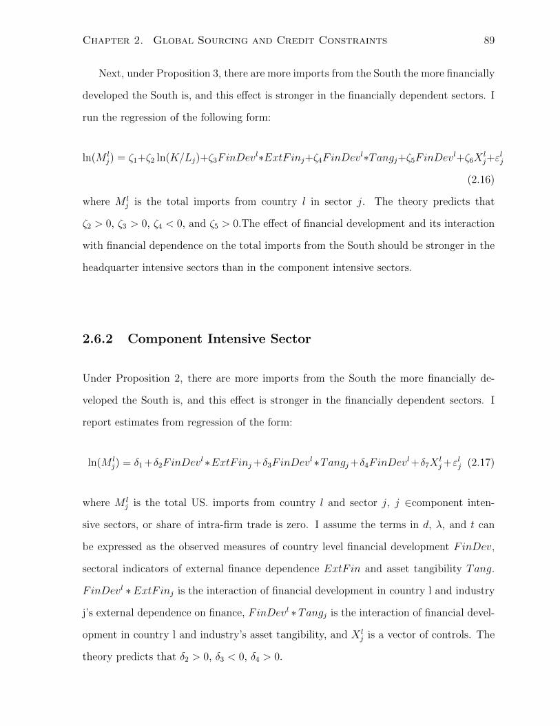
Chapter 2. Global Sourcing and Credit Constraints 89
Next, under Proposition 3, there are more imports from the South the more financially
developed the South is, and this effect is stronger in the financially dependent sectors. I
run the regression of the following form:
ln(M lj) = ζ1+ζ2 ln(K/Lj)+ζ3FinDev
l∗ExtF inj+ζ4FinDevl∗Tangj+ζ5FinDev
l+ζ6Xlj+ε
lj
(2.16)
where M lj is the total imports from country l in sector j. The theory predicts that
ζ2 > 0, ζ3 > 0, ζ4 < 0, and ζ5 > 0.The effect of financial development and its interaction
with financial dependence on the total imports from the South should be stronger in the
headquarter intensive sectors than in the component intensive sectors.
2.6.2 Component Intensive Sector
Under Proposition 2, there are more imports from the South the more financially de-
veloped the South is, and this effect is stronger in the financially dependent sectors. I
report estimates from regression of the form:
ln(M lj) = δ1 +δ2FinDev
l∗ExtF inj+δ3FinDevl∗Tangj+δ4FinDev
l+δ7Xlj+εlj (2.17)
where M lj is the total US. imports from country l and sector j, j ∈component inten-
sive sectors, or share of intra-firm trade is zero. I assume the terms in d, λ, and t can
be expressed as the observed measures of country level financial development FinDev,
sectoral indicators of external finance dependence ExtF in and asset tangibility Tang.
FinDevl ∗ExtF inj is the interaction of financial development in country l and industry
j’s external dependence on finance, FinDevl ∗Tangj is the interaction of financial devel-
opment in country l and industry’s asset tangibility, and X lj is a vector of controls. The
theory predicts that δ2 > 0, δ3 < 0, δ4 > 0.
Chapter 2. Global Sourcing and Credit Constraints 90
2.7 Data
In this section I use data on intra-firm and total U.S. imports from 90 countries and 429
sectors over the 1996-2005 period. I have also confirmed my results in a cross section
for each year. I evaluate the impact of credit constraints on the choice of organizational
form and location of supplier by regressing intra-firm trade variables on the interaction of
country level measure of financial development and industry level measure of dependence
on external finance and asset tangibility.20
2.7.1 Intra-firm and total U.S. imports data
A sector is defined as a 4-digit SIC industry. The share of intra-firm U.S. imports
Slj =RelatedljTotallj
, where Relatedlj is the U.S. reported import value from country l in sector j
that is from a related party, and Totallj is the total U.S. import from country l in sector
j.
2.7.2 Financial development data
The first measure of financial development I use is the ratio of credit banks and other
financial intermediaries to the private sector as a share of GDP, which I obtain from
Beck et al. (2000). Domestic credit has been used extensively in the finance and growth
literature (Rajan and Zingales, 1998; Braun 2003; Aghion et al. 2004). Stock market
capitalization and stock traded are also used for robustness checks, which I obtain from
the IMF.
In additional robustness checks, I use measures of the accounting standards, the risk
of expropriation, and the repudiation of contracts from Porta et al. (1998). Even though
these indices are not direct measures of the probability that financial contracts will be
20Firm-level data are not available. As a result, I cannot estimate firm productivities and interactthem with external finance dependence and financial development.
Chapter 2. Global Sourcing and Credit Constraints 91
enforced, they are good measures for the contracting environment in a country, which
allies to financial contracting as well. These indices are available for a subset of countries
and do not vary over time. Table 3, panel A summaries the cross sectional variation in
these measures.
2.7.3 External dependence on finance data
Industry-level measures of external dependence on finance and asset tangibility are con-
structed based on data for all publicly traded U.S. based companies from Compustat’s
annual industrial files based on usSIC 1987 classification. It is then converted to the SIC
4-digit industry classification system based on the concordance table provided by Jon
Haveman. A firm’s external dependence on finance is defined as capital expenditures
minus cash flow from operations divided by capital expenditures. An industry level’s
measure of external dependence on finance is the median firm’s external dependance on
finance in an industry, as proposed by Rajan and Zingales (1998). Asset tangibility is
similarly defined as the share of net property, plant and equipment in total book-value
assets for the median firm in a given industry. Both measures are constructed as aver-
ages for the 1996-2005 period, and appear very stable over time compared to indices for
1986-1995, 1980-1989, or 1966-1975 period.
2.8 Regression Results
2.8.1 Headquarter Intensive Sector
The Effect of Credit Constraints on the Multinationals’ Sourcing Decisions
The capital to labor ratio is used to measure the headquarter intensity of a sector.
Earlier papers on the role of capital labor ratios on the choice of organizational forms
also have documented that the share of intra-firm imports is significantly higher, the
Chapter 2. Global Sourcing and Credit Constraints 92
higher the capital intensity of the exporting industry j in country i (Antras (2003)).
Table 4 column 1 re-establishes this basic pattern between 90 countries and 375 sectors
in the period 1996-2005. Since capital labor ratio, external dependence on finance, and
asset tangibility do not have a time dimension, sector dummies are not included for all
subsequent analysis. Industry dummies at 3-digit classification level are included. The
results for the interaction terms are similar if sector dummies are used instead of the
measures on external finance and asset tangibility.
Column 2 is the regression results of equation (15) using the ratio of private credit to
GDP for each country as a measure of financial development. The interaction of finan-
cial development and external finance dependence enters negatively into the equation and
the interaction of financial development and asset tangibility enters positively into the
equation as predicted by the theory. This implies that North chooses more outsourcing
than integration in financially developed countries when the sectors are in need of more
external finance and have less tangible assets. Column 3-7 are the same regression results
but using different measures of financial development for robustness checks. Those in-
clude the ratio of stock capitalization to GDP, ratio of stock traded to GDP, accounting
standards, risk of expropriation, and contract repudiation. One might argue that degree
of a country’s financial development is an endogenous outcome of a country’s history,
origin of law, or some other endowment factors. Column 8 provides the IV estimation
result using the colonial origin of a country’s legal system as reported in Porta et al.
(1998) to instrument for the private credit to GDP ratio.
Table 9 Column 2 examines the economic significance of the effects of credit con-
straints on the share of intra-firm trade in the headquarter intensive sectors. Each cell
reports on the odds-ratio of the share of intra-firm trade to the share of outsourcing for
one standard deviation increase in the measure of financial development of the exporting
country in the sector at the 75th percentile of the distribution by external finance de-
pendence and asset tangibility, respectively, relative to the sector at the 25th percentile.

Chapter 2. Global Sourcing and Credit Constraints 93
The odds-ratio for the share of intra-firm trade to the share of outsourcing is 44% for one
standard-deviation increase in the private credit to GDP ratio in the more financially
dependent sectors (3rd quartile) than in the sectors are less financially dependent (1st
quartile). With the odds-ratio less than 100%, this implies the share of intra-firm trade
has decreased. More firms choose to outsource rather than vertically integrate when the
foreign country is more financially developed in sectors that are more dependent on fi-
nance. The opposite is true for the interaction between financial development and asset
tangibility. The odds-ratio is above 100% the interaction with asset tangibility. This
indicates that more firms choose integration over outsourcing when the foreign country
is more financially developed in sectors that have more tangible assets, and thus less
dependent on finance. These results confirm the first part of Proposition 1: the North
tends to choose more outsourcing instead of vertical integration when the South is more
financially developed and the sector is more financially dependent.
Table 5 provides additional robustness checks by including additional measures of
headquarter intensity and the interaction of headquarter intensity with financial devel-
opment of a country to isolate the effect of financial development and its interaction
with the financial dependence of a sector. Those include the U.S. industry research and
development at 3 digit NAICS from NS R&D in industry in 2004, the Rauch Index21,
and Lall Index22. By including additional measures of headquarter intensity and their
interaction with a country’s financial development measure, the results provided are in
Table 5 are not changed.
21Rauch (1999) classified products traded on an organized exchange as homogeneous goods. Productsnot sold on exchanges but whose benchmark prices exist were classified as reference priced; all otherproducts were deemed differentiated.
22Lall (2000) classified products by technology at the 3-digit SITC level. Low technology productstend to have stable and slow-changing technologies. High technology products tend to have advancedand fast-changing technologies, normally associated with high R&D investments. Middle technologyproducts lie somewhere in between.
Chapter 2. Global Sourcing and Credit Constraints 94
The Effect of Credit Constraints on Total U.S. Imports
Column 1 in Table 6 re-establishes the positive relationship between the capital labor
ratio and total U.S. imports as shown in Antras(2003). Under Proposition 3, there are
more imports from the South the more financially developed the South is, and this effect
is stronger in the financially dependent sectors. I test Proposition 3 by looking at the
OLS regression results of equation (16). Column 2-8 in Table 6 provide the results using
different measures of financial development. Those measures include private credit to
GDP ratio, ratio of stock capitalization to GDP, ratio of stock traded to GDP, accounting
standards, risk of expropriation, and contract repudiation. The last three measures are
time invariant and therefore are not included by themselves in the regression due to
multicollinearity with country dummies in the regression. Table 9 Column 3 examines
the economic significance of the effects of credit constraints on the total U.S. imports
in the headquarter intensive sectors. Each cell reports on how much bigger the effect of
one standard deviation increase in the measure of financial development of the exporting
country on the total U.S. imports in the sector at the 75th percentile of the distribution
by external finance dependence and asset tangibility, respectively, relative to the sector
at the 25th percentile. All results confirm the statement in Proposition 3 that the North
imports more from the South when the South becomes more financially developed, and
especially so in the financially dependent sector.
2.8.2 Component Intensive Sector
Next, I consider the sectors with zero intra-firm trade to be the component intensive
sectors. I test proposition 2 by estimating equation (17) for the effect of financial devel-
opment and its interaction with financial dependence in the component intensive sectors
using OLS specification. Later on, I will relax this assumption and consider different
K/L cut-offs to divide the data into component and headquarter intensive sectors. Table
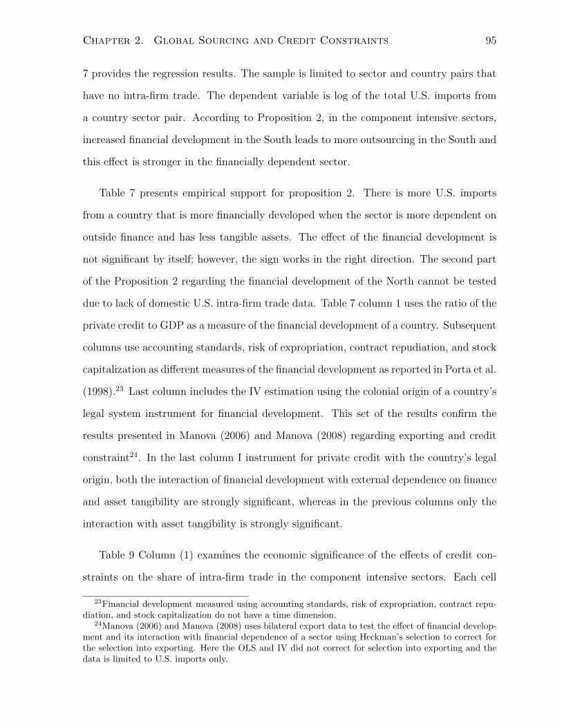
Chapter 2. Global Sourcing and Credit Constraints 95
7 provides the regression results. The sample is limited to sector and country pairs that
have no intra-firm trade. The dependent variable is log of the total U.S. imports from
a country sector pair. According to Proposition 2, in the component intensive sectors,
increased financial development in the South leads to more outsourcing in the South and
this effect is stronger in the financially dependent sector.
Table 7 presents empirical support for proposition 2. There is more U.S. imports
from a country that is more financially developed when the sector is more dependent on
outside finance and has less tangible assets. The effect of the financial development is
not significant by itself; however, the sign works in the right direction. The second part
of the Proposition 2 regarding the financial development of the North cannot be tested
due to lack of domestic U.S. intra-firm trade data. Table 7 column 1 uses the ratio of the
private credit to GDP as a measure of the financial development of a country. Subsequent
columns use accounting standards, risk of expropriation, contract repudiation, and stock
capitalization as different measures of the financial development as reported in Porta et al.
(1998).23 Last column includes the IV estimation using the colonial origin of a country’s
legal system instrument for financial development. This set of the results confirm the
results presented in Manova (2006) and Manova (2008) regarding exporting and credit
constraint24. In the last column I instrument for private credit with the country’s legal
origin, both the interaction of financial development with external dependence on finance
and asset tangibility are strongly significant, whereas in the previous columns only the
interaction with asset tangibility is strongly significant.
Table 9 Column (1) examines the economic significance of the effects of credit con-
straints on the share of intra-firm trade in the component intensive sectors. Each cell
23Financial development measured using accounting standards, risk of expropriation, contract repu-diation, and stock capitalization do not have a time dimension.
24Manova (2006) and Manova (2008) uses bilateral export data to test the effect of financial develop-ment and its interaction with financial dependence of a sector using Heckman’s selection to correct forthe selection into exporting. Here the OLS and IV did not correct for selection into exporting and thedata is limited to U.S. imports only.
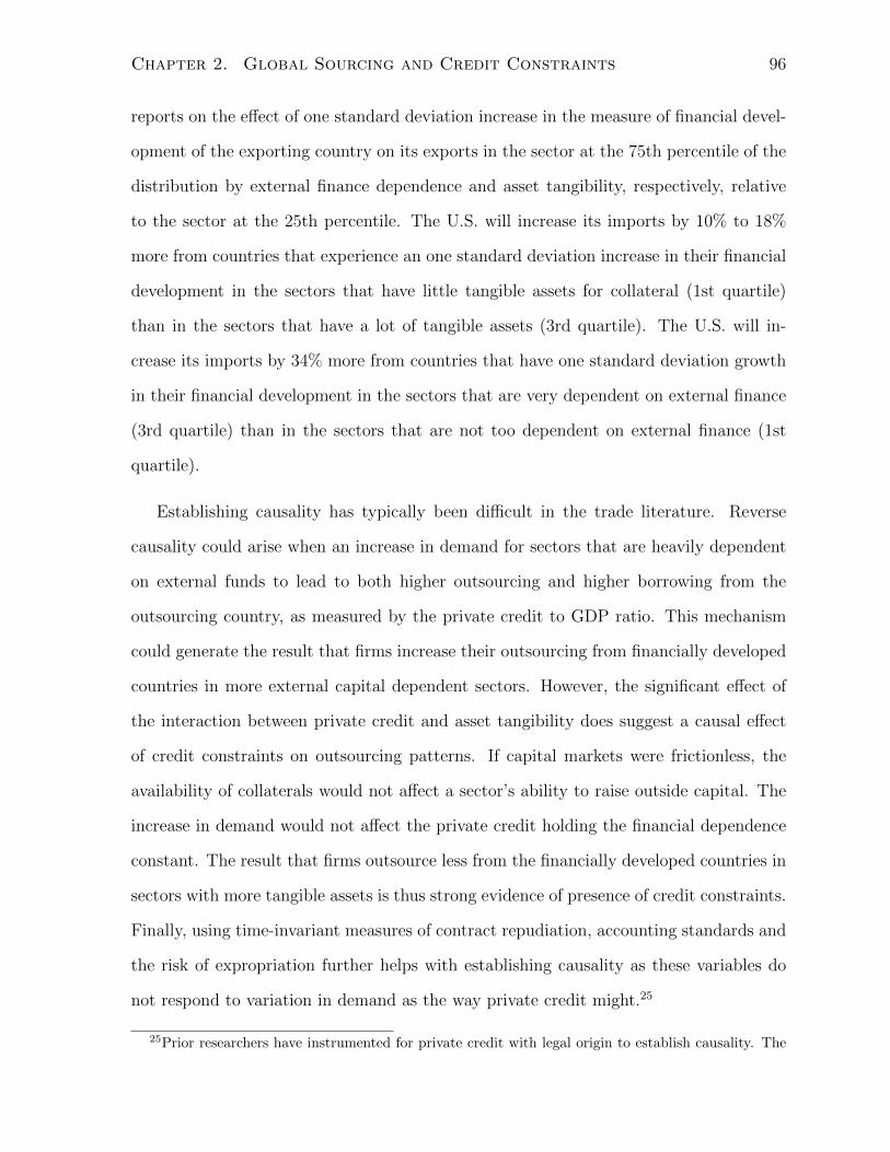
Chapter 2. Global Sourcing and Credit Constraints 96
reports on the effect of one standard deviation increase in the measure of financial devel-
opment of the exporting country on its exports in the sector at the 75th percentile of the
distribution by external finance dependence and asset tangibility, respectively, relative
to the sector at the 25th percentile. The U.S. will increase its imports by 10% to 18%
more from countries that experience an one standard deviation increase in their financial
development in the sectors that have little tangible assets for collateral (1st quartile)
than in the sectors that have a lot of tangible assets (3rd quartile). The U.S. will in-
crease its imports by 34% more from countries that have one standard deviation growth
in their financial development in the sectors that are very dependent on external finance
(3rd quartile) than in the sectors that are not too dependent on external finance (1st
quartile).
Establishing causality has typically been difficult in the trade literature. Reverse
causality could arise when an increase in demand for sectors that are heavily dependent
on external funds to lead to both higher outsourcing and higher borrowing from the
outsourcing country, as measured by the private credit to GDP ratio. This mechanism
could generate the result that firms increase their outsourcing from financially developed
countries in more external capital dependent sectors. However, the significant effect of
the interaction between private credit and asset tangibility does suggest a causal effect
of credit constraints on outsourcing patterns. If capital markets were frictionless, the
availability of collaterals would not affect a sector’s ability to raise outside capital. The
increase in demand would not affect the private credit holding the financial dependence
constant. The result that firms outsource less from the financially developed countries in
sectors with more tangible assets is thus strong evidence of presence of credit constraints.
Finally, using time-invariant measures of contract repudiation, accounting standards and
the risk of expropriation further helps with establishing causality as these variables do
not respond to variation in demand as the way private credit might.25
25Prior researchers have instrumented for private credit with legal origin to establish causality. The

Chapter 2. Global Sourcing and Credit Constraints 97
Difference in Difference Method
One of the biggest concerns of estimating the effect of financial development is deter-
mining causality. Countries that have higher export volumes have higher GDP levels,
which in turn could affect the financial institutions in those countries. In addition to
implementing the IV estimator using the colonial origin of a country’s legal system, here
I take the advantage of an exogenous event taking place that directly affects a coun-
try’s financial development. In the year 1997, the Asian financial crisis was a period
of financial crisis that gripped much of Asia and raised fears of a worldwide economic
meltdown due to financial contagion, where small shocks which initially affect only a
particular region of an economy, spread to the rest of financial sectors and other coun-
tries whose economies were previously healthy. The crisis started in Thailand with the
financial collapse of the Thai baht caused by the decision of the Thai government to
float the exchange rate for baht. Thailand became effectively bankrupt and as the crisis
spread, most of Southeast Asia and Japan saw a devalued stock market. International
investors were reluctant to lend to developing countries, leading to economic slowdowns
in developing countries in many parts of the world. By 1999, the economies of Asia were
beginning to recover. I implement the difference in difference methods before and after
the Asian financial crisis to avoid reverse causality. During the Asian financial crisis,
the financial development measures for each country falls. Table 8 shows the estimates
for the interaction between financial development and external finance dependence using
the 3 years before the Asian financial crisis and the 3 years after (the dependent vari-
able is (Sj1999 − Sj1997) − (Sj1996 − Sj1994)). Here, I took the difference between share
of intra-firm trade instead of the difference between the logs because it is easier to in-
interaction between external finance dependence and asset tangibility are strongly significant. However, ithas been argued that legal origin may impact institution formation and the economy more broadly, whichin turn are likely to affect trade through channels other than its effect on the financial development. Forrobustness checks, I use difference in difference methods around the Asian financial crisis as an exogenoussource of variation in financial development.

Chapter 2. Global Sourcing and Credit Constraints 98
terpret the difference in shares instead of the difference in logs. Using the difference in
difference method, financial contractibility in that country decreases the market share of
vertically integrated firms in that country and this effect is again more pronounced in
the financially dependent sectors.
The bottom panel in Table 9 shows the effect of countries’ financial development and
sectors’ financial dependence on firms’ sourcing decisions. During the Asian financial
crisis, the share of intra-firm trade increased by 29% in sectors that are heavily dependent
on external finance (3rd quartile) than in sectors that are less dependent on external
finance (1st quartile).
Component vs. Headquarter Intensive Sectors
As an additional robustness check, I consider different K/L cut-offs to divide the data
into component and headquarter intensive sectors. Column 1 in Table 10 provides the
regression results for equation (17) under different K/L cut-offs. Column 2 and 3 provide
the regression results for equation (15) and (16), respectively, under those K/L cut-offs.
Table 10 confirms my previous results. In addition, the magnitude of the interaction
effect between a country’s financial development and the sector’s financial dependence
are increasing as I increase the K/L cut-offs for the headquarter intensive sectors. Propo-
sition 1 states that integration is favored relative to outsourcing in sectors with higher
headquarter intensity. If K/L ratio is an accurate measure of headquarter intensity, the
reduction in the share of integration in the financially dependent sectors should be greater
when the country improved its financial development, as Column 2 in Table 10 suggests.
2.9 Conclusion
In this paper I have extended the global sourcing model ofAntras and Helpman (2004)
to incorporate the role of credit constraints. In the model, a continuum of firms with

Chapter 2. Global Sourcing and Credit Constraints 99
heterogeneous productivities decide whether to integrate or outsource the intermediate
inputs and in which countries to source the inputs. By choosing an organizational struc-
ture, the firm (final good producer or intermediate supplier depending on the choice of
organizational structure) faces a fixed cost, part of which cannot be financed internally
and needs to raise outside capital to finance it. When the financial contract is enforced,
the firms needs to make a payment to the investor; when the financial contract is not
enforced, the investors claim the collaterals of the firms. By competing for investors’
capital, some firms that could operate without credit constraint are now forced to exit
the market with credit constraint because they cannot make enough repayment to the
investors when the financial contract is enforced. The productivity cut-off level is raised
for all forms of organization under credit constraint.
This model generates equilibria in which firms with different productivity levels choose
different ownership structure and suppliers location. In the model, credit constraints af-
fect firms in different countries and sectors differently. Final-good producers in some
sectors find it easier to operate because they need to raise less outside finance and have
more tangible assets. Credit constraints vary across countries because contracts between
firms and investors are more likely to be enforced at higher levels of financial devel-
opment.In particular, I study the effect of improvements in financial contractibility on
relative prevalence of these organizational forms. I have shown that an improvement in
financial contractibility in the South decreases the market share of vertically integrated
final-good producers, this effect is more pronounced in the financially dependent sector,
i.e. the interaction of financial development and external dependence on finance has a
negative effect on the market share of vertically integrated firms, and the interaction of
financial development and asset tangibility has a positive effect on the market share of
vertically integrate firms.

Chapter 2. Global Sourcing and Credit Constraints 100
Figure 1. U.S. Intra-Firm Imports and External Financial Dependence
This graph shows the relationship betweeen the share of U.S. intra-firm imports insector j and the sector’s external dependence on finance. The share of U.S. intra-firm imports in sector j is defined as sum of all party-related U.S. imports in sectorj divided by the sum of all U.S. imports in sector j. A firm’s external dependence onfinance is defined as capital expenditures minus cash flow from operations dividedby capital expenditures. A sector’s external dependence on finance is defined asthe median firm’s external dependence on finance in that sector. All data is foryear 2000.
0.2
.4.6
.81
Sha
re o
f Int
ra-f
irm T
rade
-2 -1.5 -1Log External Finance Dependence
share Fitted values
Share of Intra-firm Trade vs External Finance Dependence
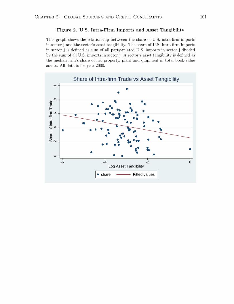
Chapter 2. Global Sourcing and Credit Constraints 101
Figure 2. U.S. Intra-Firm Imports and Asset Tangibility
This graph shows the relationship betweeen the share of U.S. intra-firm importsin sector j and the sector’s asset tangibility. The share of U.S. intra-firm importsin sector j is defined as sum of all party-related U.S. imports in sector j dividedby the sum of all U.S. imports in sector j. A sector’s asset tangibility is defined asthe median firm’s share of net property, plant and quipment in total book-valueassets. All data is for year 2000.
0.2
.4.6
.81
Sha
re o
f Int
ra-f
irm T
rade
-6 -4 -2 0Log Asset Tangibility
share Fitted values
Share of Intra-firm Trade vs Asset Tangibility

Chapter 2. Global Sourcing and Credit Constraints 102
Figure 3. Average Financial Vulnerability of Intra-firm Trade
This figure shows the average financial vulnerability of share of intra-firm trade overtime for12 countries that have improved their financial development by the measurement of privatecredit to GDP ratio by at least 20% of their 1996 level. For each year the average intensity ofintra-firm trade with respect to external finance dependence (Avg Fin Dep of S) is calculatedas∑
j FinDepj ∗ Intralj,t, where Intralj,t is the share of U.S. intra-firm imports in sector j fromcountry l in time t. The average intensity of intra-firm trade with respect to asset tangibility(Avg Tang of S) is similarly constructed. Each country graph plots Avg Fin Dep of S (Avg Tangof S) on the left (right) vertical axis. Each graph’s title indicates the difference between the logprivate credit in 1996 and 2004. The graphs are sorted by the degree of change in the financialdevelopment of a country.
.04
.06
.08
.1.1
2A
vera
ge T
ang
of S
-.20
.2.4
Ave
rage
Fin
Dep
of S
1996 1998 2000 2002 2004year
Average FinDep of S Average Tang of S
VNM, 2.01
.15
.2.2
5.3
Ave
rage
Tan
g of
S
-.2-.1
5-.1
-.05
0A
vera
ge F
inD
ep o
f S
1996 1998 2000 2002 2004year
Average FinDep of S Average Tang of S
DNK, 1.65
0.0
5.1
.15
.2.2
5A
vera
ge T
ang
of S
-.4-.2
0.2
.4.6
Ave
rage
Fin
Dep
of S
1996 1998 2000 2002 2004year
Average FinDep of S Average Tang of S
ALB, 1.35
0.1
.2.3
.4A
vera
ge T
ang
of S
-.3-.2
-.10
Ave
rage
Fin
Dep
of S
1996 1998 2000 2002 2004year
Average FinDep of S Average Tang of S
DZA, .91
.08
.1.1
2.1
4.1
6.1
8A
vera
ge T
ang
of S
-.4-.2
0.2
.4A
vera
ge F
inD
ep o
f S
1996 1998 2000 2002 2004year
Average FinDep of S Average Tang of S
MAR, .69
.2.2
2.2
4.2
6.2
8.3
Ave
rage
Tan
g of
S
-.3-.2
5-.2
-.15
-.1-.0
5A
vera
ge F
inD
ep o
f S
1996 1998 2000 2002 2004year
Average FinDep of S Average Tang of S
IRL, .58
.05
.1.1
5.2
Ave
rage
Tan
g of
S
-.3-.2
5-.2
-.15
-.1A
vera
ge F
inD
ep o
f S
1996 1998 2000 2002 2004year
Average FinDep of S Average Tang of S
POL, .52
.06
.08
.1.1
2A
vera
ge T
ang
of S
-.25
-.2-.1
5-.1
Ave
rage
Fin
Dep
of S
1996 1998 2000 2002 2004year
Average FinDep of S Average Tang of S
ESP, .43
.06
.08
.1.1
2A
vera
ge T
ang
of S
-.25
-.2-.1
5-.1
Ave
rage
Fin
Dep
of S
1996 1998 2000 2002 2004year
Average FinDep of S Average Tang of S
IND, .43
0.0
5.1
.15
.2.2
5A
vera
ge T
ang
of S
-.2-.1
5-.1
Ave
rage
Fin
Dep
of S
1996 1998 2000 2002 2004year
Average FinDep of S Average Tang of S
EGY, .39
.1.1
2.1
4.1
6A
vera
ge T
ang
of S
-.25
-.2-.1
5-.1
-.05
Ave
rage
Fin
Dep
of S
1996 1998 2000 2002 2004year
Average FinDep of S Average Tang of S
VEN, .31
0.0
5.1
.15
Ave
rage
Tan
g of
S
-.25
-.2-.1
5-.1
-.05
0A
vera
ge F
inD
ep o
f S
1996 1998 2000 2002 2004year
Average FinDep of S Average Tang of S
NIC, .26
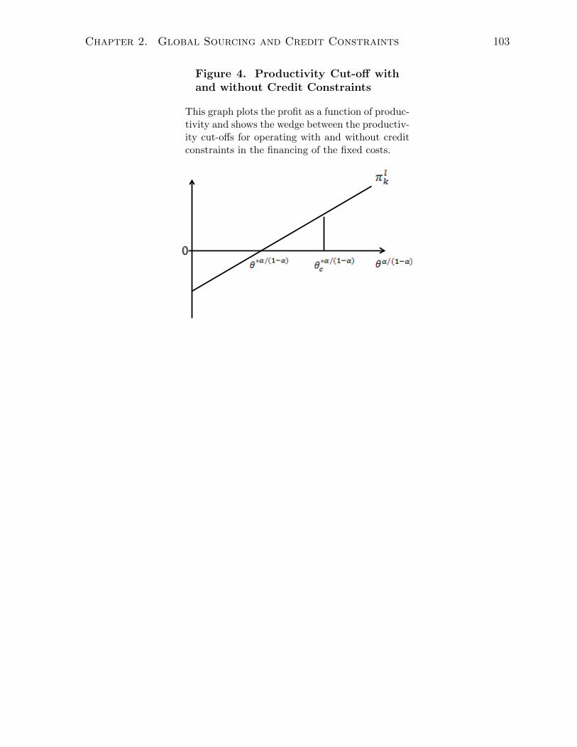
Chapter 2. Global Sourcing and Credit Constraints 103
Figure 4. Productivity Cut-off withand without Credit Constraints
This graph plots the profit as a function of produc-tivity and shows the wedge between the productiv-ity cut-offs for operating with and without creditconstraints in the financing of the fixed costs.

Chapter 2. Global Sourcing and Credit Constraints 104
Figure 5. Productivity Cut-offs inHeadquarter Intensive Sector with-out Credit Constraints
This graph plots the profit as a function of produc-tivity in the Headquarter Intensive Sector and showsthe productivity cut-offs for outsourcing in the North,vertical integration in the North, outsourcing in theSouth, and vertical integration in the South withoutcredit constraints in the financing of the fixed costs.

Chapter 2. Global Sourcing and Credit Constraints 105
Figure 6. Existence of Multinational Firms andFinancial Improvement in the South
This graph shows that different subsets of firm organizational firms may existin the equilibrium; however, vertical integration in the South will alwaysexist due to lack of the upper bound on the productivity. The arrows showhow the productivity cut-offs will change for a financial improvement in theSouth.
Exit Outsourcing in N
Outsourcing in S
Integration in N
Integration in S (FDI)
Exit Outsourcing in N
Outsourcing in S
Integration in S (FDI)
Exit Outsourcing in N
Integration in N
Integration in S (FDI)
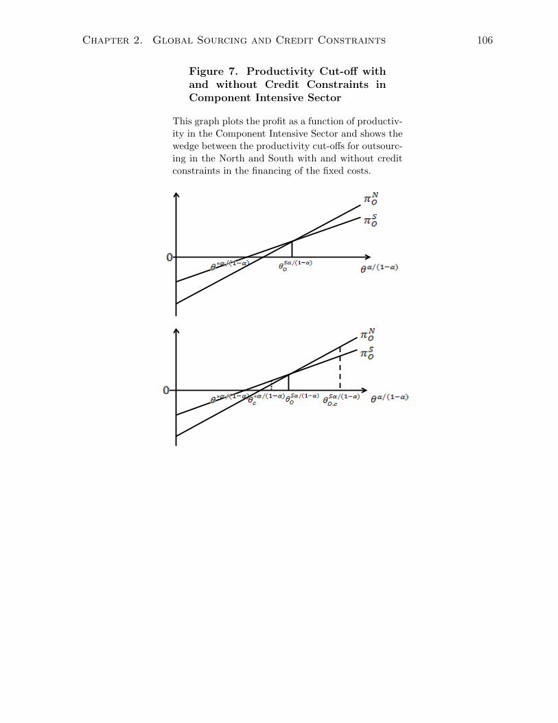
Chapter 2. Global Sourcing and Credit Constraints 106
Figure 7. Productivity Cut-off withand without Credit Constraints inComponent Intensive Sector
This graph plots the profit as a function of productiv-ity in the Component Intensive Sector and shows thewedge between the productivity cut-offs for outsourc-ing in the North and South with and without creditconstraints in the financing of the fixed costs.
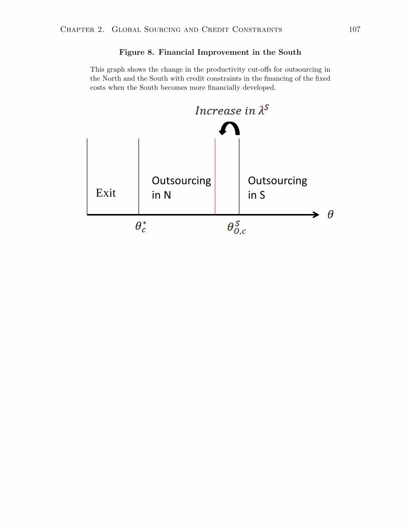
Chapter 2. Global Sourcing and Credit Constraints 107
Figure 8. Financial Improvement in the South
This graph shows the change in the productivity cut-offs for outsourcing inthe North and the South with credit constraints in the financing of the fixedcosts when the South becomes more financially developed.
Exit Outsourcing in N
Outsourcing in S
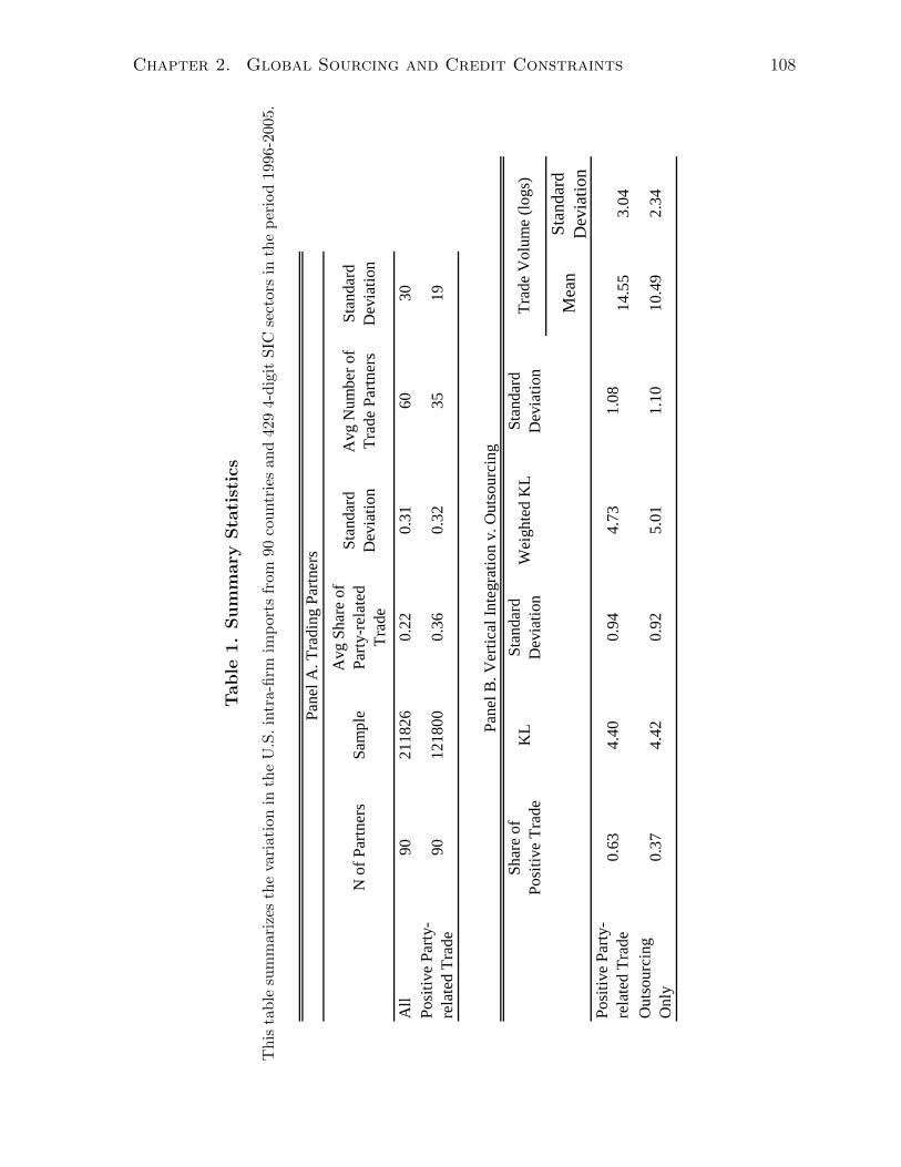
Chapter 2. Global Sourcing and Credit Constraints 108
Table
1.
Sum
mary
Sta
tist
ics
Th
ista
ble
sum
mar
izes
the
vari
atio
nin
the
U.S
.in
tra-
firm
imp
orts
from
90co
untr
ies
and
429
4-d
igit
SIC
sect
ors
inth
ep
erio
d19
96-2
005.
N o
f Par
tner
sSa
mpl
eA
vg S
hare
of
Party
-rela
ted
Trad
e
Stan
dard
D
evia
tion
Avg
Num
ber o
f Tr
ade
Partn
ers
Stan
dard
D
evia
tion
All
9021
1826
0.22
0.31
6030
Posi
tive
Party
-re
late
d Tr
ade
9012
1800
0.36
0.32
3519
Shar
e of
Po
sitiv
e Tr
ade
KL
Stan
dard
D
evia
tion
Wei
ghte
d K
LSt
anda
rd
Dev
iatio
n
Mea
nSt
anda
rd
Dev
iatio
nPo
sitiv
e Pa
rty-
rela
ted
Trad
e0.
634.
400.
944.
731.
0814
.55
3.04
Out
sour
cing
O
nly
0.37
4.42
0.92
5.01
1.10
10.4
92.
34
Pane
l A. T
radi
ng P
artn
ers
Trad
e V
olum
e (lo
gs)
Pane
l B. V
ertic
al In
tegr
atio
n v.
Out
sour
cing

Chapter 2. Global Sourcing and Credit Constraints 109
Table 2. Measurements of Financial Development
This table summarizes the variation a country’s financial development variation over thetimer period 1996–2005. The financial development is defined as the ratio of private creditto GDP.
ISO Mean St Dev ISO Mean St Dev ISO Mean St Dev
CHE 1.60 0.04 BOL 0.45 0.07 GTM 0.17 0.01HKG 1.58 0.10 SVK 0.43 0.08 TUR 0.17 0.02GBR 1.27 0.12 URY 0.42 0.13 TGO 0.15 0.01PRT 1.17 0.30 HRV 0.40 0.08 MLI 0.15 0.03DEU 1.13 0.05 SLV 0.40 0.02 HTI 0.14 0.01JPN 1.11 0.05 PHL 0.38 0.07 PNG 0.14 0.02NZL 1.07 0.07 IDN 0.31 0.17 MNG 0.13 0.08SGP 1.04 0.08 HND 0.31 0.06 RUS 0.13 0.04IRL 0.95 0.18 HUN 0.29 0.08 LTU 0.13 0.04MYS 0.95 0.06 LKA 0.28 0.01 NGA 0.13 0.03THA 0.93 0.18 BRA 0.28 0.01 MDA 0.13 0.04CHN 0.92 0.03 VNM 0.27 0.16 KAZ 0.11 0.07ESP 0.91 0.14 KEN 0.27 0.03 BFA 0.11 0.02DNK 0.89 0.57 ECU 0.27 0.06 GHA 0.10 0.02AUS 0.85 0.10 IND 0.27 0.04 VEN 0.09 0.02PAN 0.82 0.11 SAU 0.25 0.03 MOZ 0.09 0.06ISR 0.80 0.12 POL 0.24 0.04 MDG 0.09 0.01KOR 0.72 0.15 PAK 0.23 0.02 ARM 0.07 0.01ITA 0.70 0.12 PER 0.23 0.03 DZA 0.07 0.03JOR 0.68 0.02 DOM 0.23 0.04 ZMB 0.07 0.01ZAF 0.67 0.07 NIC 0.22 0.04 KHM 0.06 0.01NOR 0.67 0.08 CRI 0.21 0.07 GEO 0.06 0.02CAN 0.66 0.03 PRY 0.21 0.04 UGA 0.05 0.00SWE 0.63 0.31 JAM 0.20 0.05 ALB 0.05 0.02FIN 0.57 0.05 COL 0.19 0.02 CAF 0.05 0.01CHL 0.56 0.04 ARG 0.19 0.05 KGZ 0.05 0.02TUN 0.53 0.05 BGR 0.19 0.09 TZA 0.05 0.01GRC 0.50 0.15 LVA 0.18 0.10 NER 0.05 0.01CZE 0.49 0.15 MEX 0.18 0.03 AGO 0.03 0.01EGY 0.46 0.07 SEN 0.17 0.02 SLE 0.02 0.01

Chapter 2. Global Sourcing and Credit Constraints 110
Table 3. Measurements of Financial Developmentand Financial Vulnerability
Panel A provides the summary statistics for other financial de-velopment measures: risk of expropriation, risk of contract re-pudiation, accounting standard, and whether a country is of En-glish origin. On a scale from 1 to 10, a higher score implies lessrisk of expropriation and contract repudiation. A higher scoreon accounting standard also implies better financial development.Panel B provides the summary statistics for a sector’s externaldependence on finance and asset tangibility.
Sample Mean Standard Deviation
Risk of Expropriation 41 7.83 1.53Risk of Contract Repudiation 41 7.34 1.74Accounting Standards 34 60 14Eglish Origin 41 0.39 0.49
Sample Mean Standard Deviation
External Finance 172225 -1.25 2.04Asset Tangibility 172225 0.74 0.73
Panel A. Measures of Financial Development
Panel B. Measures of Financial Vulnerabiltiy
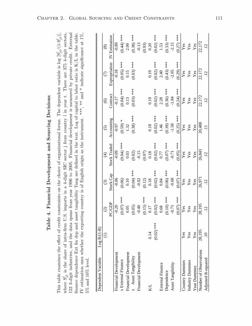
Chapter 2. Global Sourcing and Credit Constraints 111
Tab
le4.
Fin
anci
al
Develo
pm
ent
and
Sourc
ing
Deci
sions
Th
ista
ble
exam
ines
the
effec
tof
cred
itco
nst
rain
tson
the
choi
ceof
orga
niz
atio
nal
form
s.T
he
dep
end
ent
vari
able
islo
g[Sl jt
/(1-
Sl jt
)],
wh
ere
Sl jt
isth
esh
are
of
intr
a-fi
rmU
.S.
imp
orts
ina
4-d
igit
SIC
sect
orj
from
cou
ntr
yl
inye
art.
Th
ere
are
375
4-d
igit
sect
ors,
122
3-d
igit
ind
ust
ries
,an
dth
ed
ata
span
sfr
omye
ar19
96to
2005
.F
inan
cial
dev
elop
men
tis
mea
sure
dby
pri
vate
cred
it.
Exte
rnal
fin
ance
dep
end
ence
Ext
fin
dep
and
ass
etta
ngi
bil
ity
Tan
gar
ed
efin
edin
the
text.
Log
ofca
pit
alto
lab
orra
tio
isK
/Lin
the
tab
le.
IVes
tim
atio
nu
ses
wh
eth
erth
eex
port
ing
cou
ntr
yis
ofE
ngl
ish
orig
inas
the
inst
rum
ent.
***,
**an
d*
ind
icat
esi
gnifi
can
ceat
1%,
5%an
d10
%le
vel.
Dep
ende
nt V
aria
ble
Log
R/(1
-R)
(0.0
7)**
*(0
.06)
(0.0
4)**
*(0
.59)
*(0
.04)
***
(0.0
5)**
*(0
.44)
***
(0.0
5)(0
.04)
***
(0.0
2)(0
.38)
***
(0.0
3)**
*(0
.03)
***
(0.3
8)**
*Fi
nanc
ial D
evel
opm
ent
(0.1
5)**
*(0
.12)
(0.0
7)(0
.93)
K/L
(0.0
2)**
*(0
.02)
***
(0.0
2)**
*(0
.02)
***
(0.0
2)**
*(0
.02)
***
(0.0
2)**
*(0
.02)
***
(0.1
0)**
*(0
.06)
***
(0.0
7)**
*(0
.39)
***
(0.3
6)**
*(0
.43)
***
(0.3
3)**
*A
sset
Tan
gibi
lity
(0.0
7)**
*(0
.07)
***
(0.0
5)**
*(0
.25)
***
(0.2
4)**
*(0
.29)
***
(0.2
7)**
*C
ount
ry D
umm
ies
Indu
stry
Dum
mie
sY
ear D
umm
ies
Num
ber o
f Obs
erva
tions
Adj
uste
d R
-squ
ared
(7)
(8)
(1)
(2)
(3)
(4)
(5)
(6)
Fina
ncia
l Dev
elop
men
t x
Exte
rnal
Fin
ance
Fi
nanc
ial D
evel
opm
ent
x
Ass
et T
angi
bilit
y
0.14
-0.2
0
-0.7
1
0.68
0.17
-0.4
0
0.05
Exte
rnal
Fin
ance
D
epen
denc
e
26,9
71.1
226
,843
.12
20,4
88.1
1
Yes
Yes
Yes
Yes
Yes
Yes
Yes
Yes
Yes
Yes
Yes
Yes
Yes
Yes
Yes
Yes
Yes
Yes
Yes
Yes
Yes
28,1
95.1
028
,195
.12
Yes
Yes
Yes
-0.0
6
0.10
-0.0
2
0.18
0.84
-0.6
8
22,1
72.1
222
,172
.12
22,1
72.1
2
-0.0
9
0.03
-0.1
5
0.18
0.77
-0.7
1
-0.9
7
1.32
0.18
1.46
-1.5
8
-0.1
7
0.13
0.19
2.28
-1.8
4
-0.1
8
0.15
0.19
2.40
-2.0
5
-0.8
9
2.00
-0.1
3
0.20
1.53
-2.1
5
IV E
stim
atio
nPC
/GD
PSt
ock
Cap
Stoc
k Tr
aded
Acc
ount
ing
Con
tract
Ex
prop
riatio
n

Chapter 2. Global Sourcing and Credit Constraints 112T
ab
le5.
Fin
an
cial
Develo
pm
ent
and
Sourc
ing
Deci
sions:
Robust
ness
Check
s
Th
ista
ble
exam
ines
the
rob
ust
nes
sof
the
effec
tof
cred
itco
nst
rain
tson
the
choi
ceof
orga
niz
atio
nal
form
s.T
he
dep
end
ent
vari
ab
leis
log
[Sl jt
/(1-Sl jt
)],
wh
ere
Sjt
isth
esh
are
ofin
tra-
firm
U.S
.im
por
tsin
a4-
dig
itS
ICse
ctor
jfr
omco
untr
yl
inye
art.
Th
ere
are
375
4-d
igit
sect
ors
,12
23-
dig
itin
du
stri
es,
and
the
dat
asp
ans
from
yea
r19
96to
2005
.F
inan
cial
dev
elop
men
tis
mea
sure
dby
pri
vate
cred
it.
Exte
rnal
fin
ance
dep
end
ence
Ext
fin
dep
and
asse
tta
ngi
bil
ity
Tan
gar
ed
efin
edin
the
text.
Log
ofca
pit
alto
lab
orra
tio
isK
/Lin
the
tab
le.
R&
Dis
log
R&
Dfr
omU
.S.;
Lal
lin
dex
iseq
ual
toon
efo
rh
igh
-an
dm
ediu
m-t
ech
pro
du
cts,
zero
for
low
-tec
hp
rod
uct
s(L
all,
2000
);an
dR
auch
Ind
exis
equ
alto
one
ifit
’str
aded
onin
tegr
ated
mar
ket
orre
fere
nce
dp
rice
d(R
au
ch,
1999
),se
ed
etai
ld
iscu
ssio
nin
text.
***,
**an
d*
ind
icat
esi
gnifi
can
ceat
1%,
5%an
d10%
level
.
Dep
ende
nt V
aria
ble
(0.0
8)**
*(0
.03)
***
(0.0
8)(0
.03)
***
(0.0
8)**
*(0
.02)
***
(0.0
7)*
(0.0
6)
(0.0
5)(0
.04)
***
(0.0
5)(0
.04)
***
(0.0
5)(0
.04)
**(0
.05)
**(0
.05)
***
(0.0
0)(0
.00)
(0.0
0)(0
.00)
**
(0.0
4)(0
.03)
(0.0
4)(0
.03)
(0.0
6)(0
.05)
(0.0
6)(0
.05)
***
Fina
ncia
l Dev
elop
men
t(0
.15)
**(0
.13)
(0.1
5)(0
.12)
(0.1
5)**
*(0
.12)
(0.1
5)(0
.13)
R &
D(0
.01)
***
(0.0
0)**
*(0
.01)
(0.0
0)La
ll In
dex
(0.0
5)**
*(0
.04)
***
(0.0
6)**
*(0
.04)
***
Rau
ch In
dex
(0.0
9)**
*(0
.06)
***
(0.0
9)**
*(0
.06)
***
K/L
(0.0
2)**
*(0
.02)
***
(0.0
2)**
*(0
.02)
***
(0.0
2)**
*(0
.02)
***
(0.0
2)**
*(0
.02)
***
(0.1
0)**
*(0
.05)
***
(0.1
0)**
*(0
.05)
***
(0.1
0)**
*(0
.05)
***
(0.1
0)**
*(0
.06)
***
Ass
et T
angi
blity
(0.0
8)**
*(0
.05)
***
(0.0
8)(0
.06)
(0.0
8)**
*(0
.06)
***
(0.0
9)(0
.06)
Cou
ntry
Dum
mie
sIn
dust
ry D
umm
ies
Yea
r Dum
mie
sN
umbe
r of O
bser
vatio
nsA
djus
ted
R-s
quar
ed
(7)
(8)
(1)
(2)
(3)
(4)
(5)
(6)
Log
R/(1
-R)
Fina
ncia
l Dev
elop
men
t x
Exte
rnal
Fin
ance
Fi
nanc
ial D
evel
opm
ent
x
Ass
et T
ang
Fina
ncia
l Dev
elop
men
t x
R &
DFi
nanc
ial D
evel
opm
ent
x La
ll In
dex
Yes
-0.1
8
0.05
0.00
0.16
Fina
ncia
l Dev
elop
men
t x
Rau
ch In
dex
Exte
rnal
Fin
ance
D
epep
endc
e
Yes
Yes
Yes
Yes
Yes
Yes
-0.3
6
0.06
Yes
Yes
Yes
Yes
Yes
Yes
Yes
Yes
Yes
Yes
Yes
Yes
Yes
Yes
Yes
Yes
Yes
28,1
83.1
3.1
3.1
5.1
5.1
3.1
3.1
5.1
526
,964
28,1
8326
,964
28,1
8326
,964
28,1
8326
,964
0.65
-0.4
6
-0.0
7
0.12
0.00
-0.0
4
0.06
0.17
0.78
-0.4
1
-0.1
1
0.11
-0.2
1
0.05
0.48
-0.0
6
0.92
-0.0
6
0.15
-0.0
9
0.92
0.06
0.56
-0.0
6
-0.0
10.
00
-0.2
1
0.07
0.03
-0.4
2
-0.7
8
0.29
0.60
-0.4
4
0.05
0.10
0.08
-0.0
2
-0.7
4
0.28
0.78
-0.4
3
-0.1
2
0.11
0.00
-0.0
3
0.07
-0.2
0
0.00
0.86
-0.4
0
0.13
0.45
0.04
-0.0
1
0.15
0.01
-0.0
3
0.13
-0.1
5
0.00
0.86
-0.3
8
0.13
0.57
0.03
Priv
ate
Cre
dit
Stoc
k C
apPr
ivat
e C
redi
tSt
ock
Cap
Priv
ate
Cre
dit
Stoc
k C
apPr
ivat
e C
redi
tSt
ock
Cap
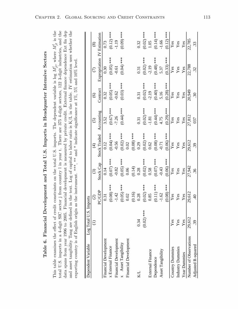
Chapter 2. Global Sourcing and Credit Constraints 113
Tab
le6.
Fin
an
cial
Develo
pm
ent
and
Tota
lU
.S.
Imp
ort
sin
Headquart
er
Inte
nsi
ve
Sect
ors
Th
ista
ble
exam
ines
the
effec
tof
cred
itco
nst
rain
tson
the
tota
lU
.S.
imp
orts
.T
he
dep
end
ent
vari
able
islo
gM
l jt,
wh
ereM
l jtis
the
tota
lU
.S.
imp
ort
sin
a4-
dig
itS
ICse
ctor
jfr
omco
untr
yl
inye
art.
Th
ere
are
375
4-d
igit
sect
ors,
122
3-d
igit
ind
ust
ries
,an
dth
ed
ata
span
sfr
omye
ar199
6to
2005
.F
inan
cial
dev
elop
men
tis
mea
sure
dby
pri
vate
cred
it.
Exte
rnal
fin
ance
dep
end
ence
Ext
fin
dep
and
ass
etta
ngi
bil
ity
Tan
gar
ed
efin
edin
the
text.
Log
ofca
pit
alto
lab
orra
tio
isK
/Lin
the
tab
le.
IVes
tim
atio
nu
ses
wh
eth
erth
eex
port
ing
cou
ntr
yis
of
En
glis
hori
gin
as
the
inst
rum
ent.
***,
**an
d*
ind
icat
esi
gnifi
can
ceat
1%,
5%an
d10
%le
vel.
Dep
ende
nt V
aria
ble
Log
Tota
l U.S
. Im
ports (0.0
8)**
*(0
.07)
***
(0.0
4)**
*(0
.67)
***
(0.0
5)**
*(0
.05)
***
(0.1
2)**
*
(0.0
5)**
*(0
.05)
***
(0.0
2)**
*(0
.44)
***
(0.0
3)**
*(0
.04)
***
(0.0
9)**
*Fi
nanc
ial D
evel
opm
ent
(0.1
6)(0
.14)
(0.0
8)**
*K
/L(0
.02)
***
(0.0
2)**
*(0
.02)
***
(0.0
2)**
*(0
.02)
***
(0.0
2)**
*(0
.02)
***
(0.0
2)**
*
(0.1
1)**
*(0
.07)
***
(0.0
8)**
*(0
.44)
***
(0.4
0)**
*(0
.48)
***
(0.1
4)**
*A
sset
Tan
gibi
lity
(0.0
8)**
*(0
.06)
***
(0.0
6)**
*(0
.29)
***
(0.2
8)**
*(0
.33)
***
(0.1
2)**
*C
ount
ry D
umm
ies
Indu
stry
Dum
mie
sY
ear D
umm
ies
Num
ber o
f Obs
erva
tions
Adj
uste
d R
-squ
ared
(7)
(8)
(1)
(2)
(3)
(4)
(5)
(6)
PC/G
DP
Stoc
k C
apSt
ock
Trad
edA
ccou
ntin
g C
ontra
ct
Expr
opria
tion
IV E
stim
atio
nFi
nanc
ial D
evel
opm
ent
x Ex
tern
al F
inan
ce
Fina
ncia
l Dev
elop
men
t x
A
sset
Tan
gibi
lity
Exte
rnal
Fin
ance
D
epen
denc
e
Yes
Yes
Yes
Yes
Yes
Yes
Yes
Yes
Yes
Yes
Yes
Yes
Yes
Yes
Yes
Yes
Yes
Yes
Yes
Yes
Yes
Yes
Yes
Yes
29,6
12.3
929
,612
.40
27,9
42.3
629
,612
.39
27,8
1203
720
,949
.30
22,7
88.3
222
,785
.33
0.34
0.31
-1.4
2
0.02
0.28
0.85
-1.6
2
0.14
-0.8
2
0.06
0.28
0.58
-0.4
3
0.12
-0.5
6
0.02
0.29
0.62
-0.7
1
3.52
-7.2
6
0.31
-1.8
1
4.75
0.32
-0.6
2
0.31
-2.1
9
5.16
0.30
-0.6
1
0.31
-2.1
9
5.37
0.73
-1.1
9
0.32
1.05
-1.6
6

Chapter 2. Global Sourcing and Credit Constraints 114
Table
7.
Fin
an
cial
Develo
pm
ent
and
Tota
lU
.S.
Imp
ort
sin
Com
ponent
Inte
nsi
ve
Sect
ors
Th
ista
ble
exam
ines
the
effec
tof
cred
itco
nst
rain
tson
the
tota
lU
.S.
imp
orts
.T
he
dep
end
ent
vari
able
islo
gM
l jt,
wh
ereM
l jtis
the
tota
lU
.S.
imp
orts
ina
4-d
igit
SIC
sect
orj
from
cou
ntr
yl
inye
art.
Th
ere
are
544-
dig
itse
ctors
,7
3-d
igit
ind
ust
ries
,an
dth
ed
ata
span
sfr
omye
ar19
96to
2005
.F
inan
cial
dev
elop
men
tis
mea
sure
dby
pri
vate
cred
it.
Exte
rnal
fin
ance
dep
end
ence
Ext
fin
dep
and
asse
tta
ngi
bil
ity
Tan
gar
ed
efin
edin
the
text.
Log
ofca
pit
alto
lab
orra
tio
isK
/Lin
the
tab
le.
IVes
tim
atio
nu
ses
wh
eth
erth
eex
por
tin
gco
untr
yis
of
En
glis
hori
gin
asth
ein
stru
men
t.**
*,**
and
*in
dic
ate
sign
ifica
nce
at1%
,5%
and
10%
leve
l.
Dep
ende
nt V
aria
ble
Log
U.S
. Im
ports
(0.0
6)(0
.71)
(0.0
6)(0
.05)
(0.0
2)(0
.45)
***
(0.0
4)**
*(0
.51)
***
(0.0
4)**
*(0
.03)
***
(0.0
4)**
*(0
.34)
***
Fina
ncia
l Dev
elop
men
t(0
.13)
(2.3
0)C
ount
ry D
umm
ies
Prod
uct D
umm
ies
Yea
r Dum
mie
sN
umbe
r of O
bser
vatio
nsA
djus
ted
R-s
quar
ed
Fina
ncia
l Dev
elop
men
t x
Exte
rnal
Fin
ance
Fi
nanc
ial D
evel
opm
ent
x
Ass
et T
angi
bilit
y
Priv
ate
Cre
dit/G
DP
Acc
ount
ing
Stan
dard
sR
isk
of
Expr
opria
tion
Con
tract
R
epud
iatio
n0.
06
-0.2
7
0.02
-0.1
6
Stoc
k C
apita
lizat
ion
IV E
stim
atio
n
Yes
Yes
Yes
Yes
Yes
Yes
Yes
Yes
Yes
Yes
Yes
Yes
Yes
Yes
Yes
Yes
Yes
.28
16,0
996,
630
.26
8,16
3.2
6
Yes
8,16
3.2
612
,849
.27
8,16
3.2
6
0.12
-0.1
7
-1.8
2
0.07
-0.2
0
1.35
-1.2
6
1.13
0.03
-0.1
1
(1)
(2)
(3)
(4)
(5)
(6)

Chapter 2. Global Sourcing and Credit Constraints 115
Table 8. Difference in Difference for Financial Develop-ment and Sourcing Decisions
This table examines the effect of credit constraints on the total U.S. imports using differ-ence in difference method. The dependent variable is (Sj1999 - Sj1997) - (Sj1996- Sj1994),where Rjt is the share of intra-firm U.S. imports in a 4-digit SIC sector j from countryl in year t. There are 375 4-digit sectors, 122 3-digit industries. Because the data forthe year 1995 are not available, the data used in all previous tables only begin from 1996.However, the data are available for 1994. Difference in difference method is applied here tolook at the effec tof an exogenous event on multinational firms’ export behaviors, namelythe Asian financial crisis in the year 1997. Financial development is measured by privatecredit. External finance dependence Ext fin dep and asset tangibility Tang are defined inthe text. Log of capital to labor ratio is K/L in the table. IV estimation uses whether theexporting country is of English origin as the instrument. ***, ** and * indicate significanceat 1%, 5% and 10% level.
Dependent Variable Difference in Difference of Share of Intra-firm Trade
(0.03) *** (0.03) ** (0.01) *** (0.01) ***
(0.04) (0.04) (0.01) (0.01) ***Financial Development
(0.10) ** (0.03) *K/L
(0.02) *** 0.02 *** (0.02) *** 0.02 ***
(0.00) (0.00) **Asset Tangibility
(0.00) (0.00)Industry DummiesNumber of ObservationsR-squaredAdjusted R-squared
No Yes No Yes
-0.05
0.07
0.01
0.00
-0.02
0.00
0.08
-0.02
0.00
.0041 .0338 .0050 .0324
-0.07
0.06
-0.24
0.07
0.00)
0.00
(2)Stock Cap
5,087.0053
5,087.0792
4,657.0063
4,657.0708
Financial Development x External Finance Financial Development x Asset Tangibility
External Finance Dependence
(1)PC/GDP
-0.07
0.05
0.08

Chapter 2. Global Sourcing and Credit Constraints 116
Table 9. Economic Significance
This table examines the economic significance of the effects of credit constraints on theshare of intra-firm trade in the component intensive sectors. Each column reports theeffect of one standard deviation increase in the measure of financial development of theexporting country in the sector at the 75th percentile of the distribution by externalfinance dependence and asset tangibility, respectively, relative to the sector at the 25thpercentile. Insignificant results are not reported.
Component Intensive Sectors
One Standard Deviation Increase in the Financial Development
Total U.S. Imports
Share of Intra-firm Trade (odds ratio)
Total U.S. Imports
(1) (2) (3)External Finance Dependence 44% 22%
Asset Tangibility -11% -57%External Finance Dependence 58% 33%
Asset Tangibility -10% 205% -39%External Finance Dependence 33% 32%
Asset Tangibility -12% 250% -37%External Finance Dependence 30% 38%
Asset Tangibility -11% 247% -43%External Finance Dependence 13%
Asset Tangibility -14% 170% -44%External Finance Dependence 34% 27% 18%
Asset Tangibility -18% 360% -17%
Share of Intra-firm Trade
External Finance Dependence
- 29% -
Asset Tangibility - -
Private Credit
Accounting Standards
Headquarter Intensive Sectors
Difference in Difference
Differential Effect between sectors at 75th percentile and 25th percentile
Risk of Expropriation
Contract Repudiation
Stock Capitalization
IV

Chapter 2. Global Sourcing and Credit Constraints 117
Table 10. K/L Cut-offs for Component and Head-qurater Intensive Sectors
This table provides the regressions results for equation (5.1) (5.2) and(5.3) using prive credit to GDP ratio as the financial development measureunder different K/L cut-offs for Component and Headquarter IntensiveSectors. Column (1) reports the the results in Table 4 (1) using differentK/L cut-offs. Column (2) reports Table 5 (2) using differentK/L cut-offs.Column (3) reports Table 7 (2) using different K/L cut-offs.
(0.04) (0.02) *** (0.01) ***
(0.06) (0.03) *** (0.02) ***Financial Development
(0.24) (0.08) *** (0.07)
(0.03) *** (0.02) *** (0.01) ***
(0.05) *** (0.03) *** (0.02) ***Financial Development
(0.15) (.08)
(0.02) *** (.02) *** (0.02) ***
(.02) *** (.05) *** (0.04) ***Financial Development
(0.10) ** (0.11) *** (.10) ***0.19 -0.28 .46
Private Credit x External Finance
0.04 -0.20 0.34
Private Credit x Asset Tangibility
-0.20 0.25 -1.75
K/L top 75%Private Credit x External Finance Private Credit x Asset Tangibility
K/L top 50%
K/L bottom 25%
K/L bottom 50%
0.22
0.03 0.08
-0.64
0.12
-0.20
-0.15
0.20
(1) (2) (3)
Headquarter Intensive Sectors
K/L top 90%
Component Intensive Sectors
K/L bottom 10%-0.05
0.20
-0.19
0.20
-0.53
0.07
Private Credit x External Finance Private Credit x Asset Tangibility
0.07
-.07
.01

Chapter 2. Global Sourcing and Credit Constraints 118
Appendix
Cut-off Productivies for Headquarter Intensive Sectors
As in Antras and Helpman (2004), the cutoffs without credit contraint are given by:
θ∗ = X(α−κ)/α
[wNfNOψNO (η)
](1−α)/α
,
θNV = X(α−κ)/α
[wN(fNV − fNO )
ψNV (η)− ψNO (η)
](1−α)/α
,
θSO = X(α−κ)/α
[wN(fSO − fNV )
ψSO(η)− ψNV (η)
](1−α)/α
,
θSV = X(α−κ)/α
[wN(fSV − fSO)
ψSV (η)− ψSO(η)
](1−α)/α
,
With credit constraints, the new cutoffs are given by equation (3.13):
θ∗c = X(α−κ)/α
[(1− d+ d/λN)wNfNO − 1−λN
λNtwNfE
ψNO (η)
](1−α)/α
θNV,c = X(α−κ)/α
[(1− d+ d/λN)wN(fNV − fNO )
ψNV (η)− ψNO (η)
](1−α)/α
θSO,c = X(α−κ)/α
(1− d+ d/λS)wNfSO − 1−λSλS
twNfE −[(1− d+ d/λN)wNfNV − 1−λN
λNtwNfE
]ψSO(η)− ψNV (η)
(1−α)/α
θSV,c = X(α−κ)/α
(1− d+ d/λN)wNfSV − 1−λNλN
twNfE −[(1− d+ d/λS)wNfSO − 1−λS
λStwNfE
]ψSV (η)− ψSO(η)
(1−α)/α

Chapter 2. Global Sourcing and Credit Constraints 119
Proof of Proposition 1
In component intensive sectors, firms do not integrate. An increase in financial devel-
opment in the South leads to more outsourcing in the South (∂θSO,c∂λS
< 0 and ∂θ∗c∂λS
= 0).
An increase in financial development in the North leads to less outsourcing in the South
(∂θSO,c∂λN
> 0 and ∂θ∗c∂λN
< 0). This effect is stronger in the sectors that require more outside
capital (∂θSO,c∂d∂λS
< 0 and ∂θ∗c∂d∂λS
= 0 for the South,∂θSO,c∂d∂λN
> 0 and ∂θ∗c∂d∂λN
< 0 for the North )
and less tangible assets (∂θSO,c∂t∂λS
> 0 and ∂θ∗c∂d∂λS
= 0 for the South,∂θSO,c∂t∂λN
< 0 and ∂θ∗c∂t∂λN
> 0
for the North).
Since X and ψlk(η) is not a function of λ, d, and t, the productivity cut-off increases
if the partial derivative sign is positive, and decreases if it is negative:
∂θ∗c∂λN
∝ (tfE − dfNO
λN2)wN/ψNO < 0,
∂θ∗c∂λS
= 0
∂θSO,c∂λN
∝ − ∂θ∗c∂λN
> 0,∂θSO,c∂λS
∝ (tfE − dfSO
λS2)wN/(ψSO(η)− ψNO (η)) < 0.
∂θ∗c∂d∂λN
∝ − 1
λN2wNfNO /ψ
NO < 0,
∂θ∗c∂d∂λS
= 0
∂θSO,c∂d∂λN
> 0,∂θSO,c∂d∂λS
∝ − 1
λS2wNfSO/ψ
SO < 0,
and the opposite for tangible assets:
∂θ∗c∂t∂λN
∝1
λN2wNfNO /ψ
NO > 0,
∂θ∗c∂d∂λS
= 0
∂θSO,c∂t∂λN
< 0,∂θSO,c∂t∂λS
∝1
λS2wNfSO/ψ
SO > 0.

Chapter 2. Global Sourcing and Credit Constraints 120
Proof of Proposition 2
For headquarter intensive sectors, firms tend to choose outsourcing in more financially
developed country (∂θSV,c∂λS
> 0,∂θSO,c∂λS
< 0 and∂θSV,c∂λN
< 0,∂θSO,c∂λN
> 0). This effect is more
pronounced in financially vulnerable sectors (∂θSV,c∂d∂λS
> 0,∂θSO,c∂d∂λS
< 0,∂θSV,c∂t∂λS
< 0,∂θSO,c∂t∂λS
> 0
and∂θSV,c∂d∂λN
< 0,∂θSO,c∂d∂λN
> 0,∂θSV,c∂t∂λN
> 0,∂θSO,c∂t∂λN
< 0). In sectors with higher headquarter
intensity, integration is favored relative to outsourcing ( ∂∂η
ψlV (η)
ψlO(η)> 0 for l = N,S).
Productivity cut-offs without credit constraints in headquarter intensive sectors are
the following:
θ∗ = X(α−κ)/α
[wNfNOψNO (η)
](1−α)/α
,
θNV = X(α−κ)/α
[wN(fNV − fNO )
ψNV (η)− ψNO (η)
](1−α)/α
,
θSO = X(α−κ)/α
[wN(fSO − fNV )
ψSO(η)− ψNV (η)
](1−α)/α
,
θSV = X(α−κ)/α
[wN(fSV − fSO)
ψSV (η)− ψSO(η)
](1−α)/α
.
With credit constraints, the new cutoffs are given by:
θ∗c = X(α−κ)/α
[(1− d+ d/λN)wNfNO − 1−λN
λNtwNfE
ψNO (η)
](1−α)/α
θNV,c = X(α−κ)/α
[(1− d+ d/λN)wN(fNV − fNO )
ψNV (η)− ψNO (η)
](1−α)/α
θSO,c = X(α−κ)/α
(1− d+ d/λS)wNfSO − 1−λSλS
twNfE −[(1− d+ d/λN)wNfNV − 1−λN
λNtwNfE
]ψSO(η)− ψNV (η)
(1−α)/α
θSV,c = X(α−κ)/α
(1− d+ d/λN)wNfSV − 1−λNλN
twNfE −[(1− d+ d/λS)wNfSO − 1−λS
λStwNfE
]ψSV (η)− ψSO(η)
(1−α)/α
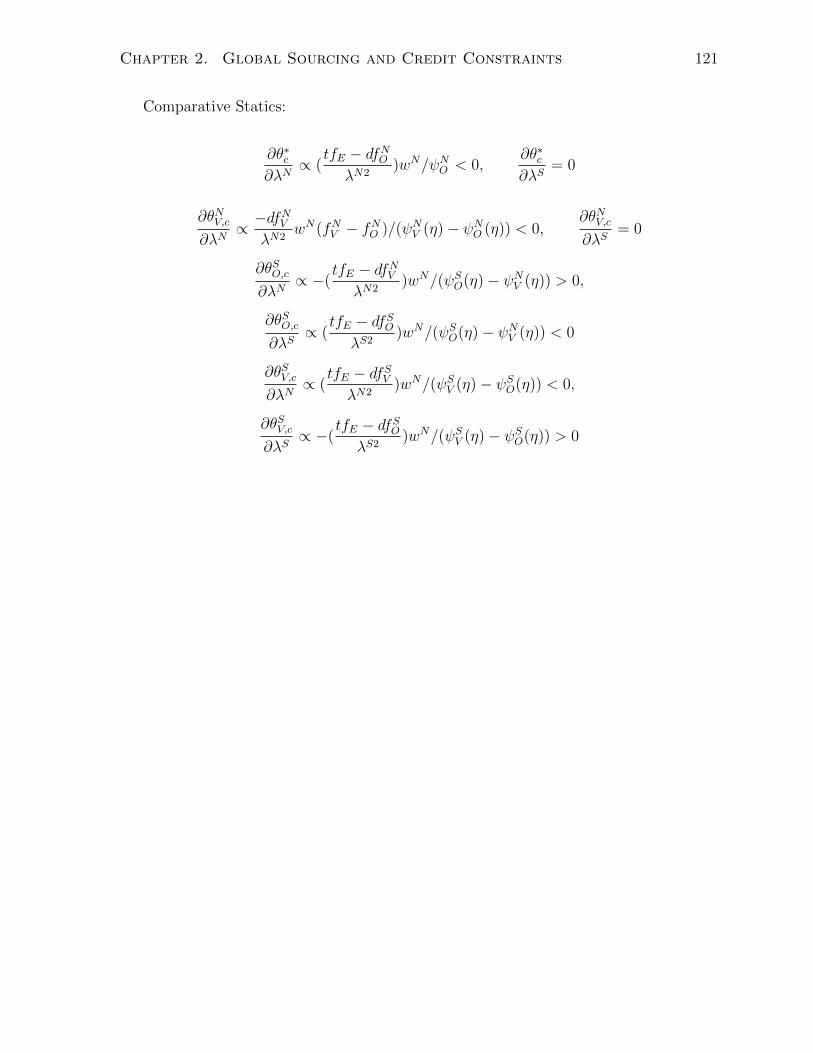
Chapter 2. Global Sourcing and Credit Constraints 121
Comparative Statics:
∂θ∗c∂λN
∝ (tfE − dfNO
λN2)wN/ψNO < 0,
∂θ∗c∂λS
= 0
∂θNV,c∂λN
∝ −dfNV
λN2wN(fNV − fNO )/(ψNV (η)− ψNO (η)) < 0,
∂θNV,c∂λS
= 0
∂θSO,c∂λN
∝ −(tfE − dfNV
λN2)wN/(ψSO(η)− ψNV (η)) > 0,
∂θSO,c∂λS
∝ (tfE − dfSO
λS2)wN/(ψSO(η)− ψNV (η)) < 0
∂θSV,c∂λN
∝ (tfE − dfSVλN2
)wN/(ψSV (η)− ψSO(η)) < 0,
∂θSV,c∂λS
∝ −(tfE − dfSO
λS2)wN/(ψSV (η)− ψSO(η)) > 0

Chapter 3
Financial Dependence and Growth
122

Chapter 3. Financial Dependence and Growth 123
3.1 Introduction
There has been a growing literature on financial institutions and growth. Dating as
far back as Schumpeter (1911), development of a country’s financial institutions has a
positive influence on the rate of growth of its per capita income. In addition, Rajan and
Zingales (1998) show that this effect is more pronounced in the financially dependent
industries.
The basic specification in this paper is a semiparametric growth rate function where
the interaction between external financial dependence of an industry and financial devel-
opment of a country enters non-parametrically and the remaining variables are paramet-
ric. This paper provides evidence that the effect of financial development and external
dependence on finance is non-linear and increasing at decreasing rate. In other words,
parametric estimation of this interaction effect significantly underestimates the effect
of financial improvement for countries starting out with low financial development and
industries that depend on less external finance, and overestimates the effect of finan-
cial improvement for countries that are already financially developed and industries that
depend on more external finance.
This non-linear effect of financial development and external finance dependence on
industry growth rates is evident in the case of China. China’s measures of financial devel-
opment, such as private credit to GDP ratio and market capitalization ratio, have grown
over the years but initially started from a low point. The fastest expanding industries in
China are the apparel and footwear industries, which are less dependent on external fi-
nance. China’s story confirms the result that financially underdeveloped countries should
focus on producing products that are less dependent on external finance while they are
improving their financial institutions. Countries that are financially underdeveloped tend
to be low and middle income countries. Sutton and Trefler (2011) also find that low and
middle income countries can achieve higher GDP growth by improving on what they are
already producing (i.e. low-tech products like footwear and textiles that tend to be not

Chapter 3. Financial Dependence and Growth 124
dependent on external finance) instead of copying what the rich countries are producing
(high-tech products).
This paper also shows that welfare effects of positive shocks to the economy are
substantially different if one estimates this financial development and external finance
dependence effect non-parametrically rather than parametrically.
Finally, this paper considers the possibility that measures of financial development
for a country are endogenous. Countries that have higher growth rates are more likely to
have better financial institutions in place. One might therefore expect the measures of
financial development to be positively correlated with the residual in an equation where
the dependent variable is growth rates or value added. In the concluding section this
paper conducts a simple test of the endogeneity hypothesis.
In summary, I have two main objectives: to estimate a semiparametric model of
growth rate in value added using the Industrial Statistics Yearbook database put together
by the United Nations Statistical Division (1993); and to test whether our measure
of financial development is endogenous. Section 2 describes the model and provides
additional details about the data. Section 3 uses single-equation differencing techniques
(Yatchew (1997), Yatchew (1998), and Yatchew (1999)) to analyze the effect of external
financial dependence and financial development on growth rates. Section 4 reports results.
Section 5 utilizes the panel data and reports semiparametric results using time changing
measurements of financial development and external finance, and the concluding Section
5 compares the results in this paper to those of previous studies.
3.2 Model and Data
This paper uses the dataset provided by Rajan and Zingales (1998). Growth in value
added for an industry is defined as the change in the log of real value added in that
industry between 1980 and 1990. External financial dependence of an industry is mea-

Chapter 3. Financial Dependence and Growth 125
sured as the median firms capital expenditures minus cash flow from operations divided
by capital expenditures in that industry. There are several measures available for finan-
cial development of a country. The first measure this paper uses is fairly traditionalthe
ratio of domestic credit plus stock market capitalization to GDP. The second proxy for
financial development used in this paper is the accounting standards in a country. A
higher score in the accounting standards indicates more disclosure.
The main empirical objective of this paper is to estimate the effect of external finan-
cial dependence on financial development on the growth rates. A priori, the relationship
between growth rates and external financial dependence interacted with financial devel-
opment maybe flat, increasing, decreasing or U-shaped; it may be concave or it may have
multiple inflection points. I propose therefore to estimate the effect using a semipara-
metric model.
In addition to an industrys external financial dependence and a countrys financial
development, a number of variables may influence growth rates and therefore need to
be incorporated into the model. These covariates include the conventional arguments of
growth rate functionan industrys share of manufacturing in a country, country indicators
and industry indicators.
The basic econometric specification is given by:
Growthjk = f(ExtF inDepj ∗ FinDevk)
+β1ShareofManufacturingjk
+β2CountryIndicators+ β3IndustryIndicators+ constant+ εjk.(3.1)
I assume little about the function beyond smoothness, thus equation (1) is a growth
rate function with the interaction between external financial dependence and financial
development entering both non-parametrically (through ) and parametrically (through
the country and industry indicators). The model has a partial linear structure y =
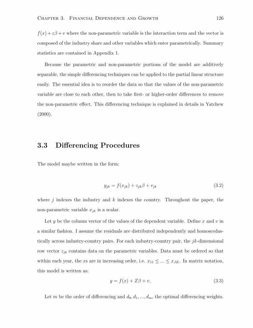
Chapter 3. Financial Dependence and Growth 126
f(x) + zβ+ v where the non-parametric variable is the interaction term and the vector is
composed of the industry share and other variables which enter parametrically. Summary
statistics are contained in Appendix 1.
Because the parametric and non-parametric portions of the model are additively
separable, the simple differencing techniques can be applied to the partial linear structure
easily. The essential idea is to reorder the data so that the values of the non-parametric
variable are close to each other, then to take first- or higher-order differences to remove
the non-parametric effect. This differencing technique is explained in details in Yatchew
(2000).
3.3 Differencing Procedures
The model maybe written in the form:
yjk = f(xjk) + zjkβ + vjk (3.2)
where j indexes the industry and k indexes the country. Throughout the paper, the
non-parametric variable xjk is a scalar.
Let y be the column vector of the values of the dependent variable. Define x and v in
a similar fashion. I assume the residuals are distributed independently and homoscedas-
tically across industry-country pairs. For each industry-country pair, the jk-dimensional
row vector zjk contains data on the parametric variables. Data must be ordered so that
within each year, the xs are in increasing order, i.e. x11 ≤ ... ≤ xJK . In matrix notation,
this model is written as:
y = f(x) + Zβ + v. (3.3)
Let m be the order of differencing and d0, d1, ..., dm, the optimal differencing weights.

Chapter 3. Financial Dependence and Growth 127
The weights satisfy the conditions:
m∑j=0
dj = 0,m∑j=0
d2j = 1 (3.4)
To estimate the parametric effects using differencing, I reorder the data so that the
values of the nonparametric variable are close. I then difference the data to remove the
effect of the nonparametric variable and run ordinary least squares regressions of the
differenced dependent variable on the differenced parametric explanatory variables. For
details on these techniques see Yatchew (1997) and Yatchew (1999).
3.4 Emprical Results
Differencing estimates of the parametric component of equation (1) are presented in Table
1 (throughout the paper I use third-order differencing (m = 3). Results for other orders
of differencing were similar.) Since I use U.S. data to identify the external dependence,
I drop the United States in all regressions. I start with private credit to GDP ratio as
the proxy for financial development. The estimated industry share effect is negative and
significant. The rest of the columns of the table include different measures of financial
development.
For comparison purposes I provide estimates of the parametric analogues of the mod-
els in Table 2. These are the different measures of financial development where the
interaction term external finance dependence and financial development is modeled us-
ing a quadratic. Estimates for different specifications of financial development do not
differ substantially between parametric and semiparametric versions. The R2, which is
defined as R2 = 1 − s2v/s
2y is higher in the semiparametric specifications relative to the
pure parametric ones.
Returning to the semiparametric specification, I remove the estimated parametric
effect from the dependent variable and analyze the non-parametric effect. I use the

Chapter 3. Financial Dependence and Growth 128
estimates from the private credit to GDP ratio to remove the parametric effect. Figure
1 displays the ordered pairs (yjk − zjkβ, xjk) as well as kernel estimates of f bordered
by 95% uniform hypotheses may be tested against non-parametric alternatives using the
static:
(mN)1/2 s2res − s2
v
s2v
→ N(0, 1) (3.5)
under H0, where s2res is the estimate of the residual variance from the parametric regres-
sion. When I insert a constant function for f equation (5) constitutes a test of significance
of the scale variable against a non-parametric alternative. The resulting test statistic is
10.89 indicating a strong scale effect of external finance dependence and financial devel-
opment on growth. Next I test a quadratic model for the interaction term. The resulting
statistics is 5.80, suggesting that the quadratic model is still inadequate.
For robustness I repeated my estimation and inference procedures using various or-
ders of differencing. Parameter estimates changed little and tests of significance and
specification were consistent with the conclusions above.
It is possible that measures of financial development for a country are endogenous.
Countries that have higher growth rates are more likely to have better financial insti-
tutions in place. One might therefore expect the measures of financial development to
be positively correlated with the residual in an equation where the dependent variable
is growth rates or value added. This in turn would lead to underestimation of the effect
of external financial dependence and financial development. Porta et al. (1998) suggests
that the origin of a countrys legal system has an effect on the development of a domestic
capital market and on the nature of the accounting system. Countries colonized by the
British tend to have sophisticated accounting system while countries colonized by the
French tend to have poor standards. This suggests using colonial origin of a countrys
legal system as one instrument. The second instrument I use is rule of law, an index of
efficiency and integrity of legal system produced by Business International Corporation,
a country-risk rating agency. I modify the specification in equation (1) to allow for a

Chapter 3. Financial Dependence and Growth 129
simple form of endogeneity as follows:
y = f(ExtF inDep ∗ FinDev) + ηγ + zβ + v (3.6)
where η is defined by the instrumental variable equation FinDev = Instrument∗π+η
and E(v|ExtF inDep ∗ FinDev, η, z) = 0 (See Blundell and Duncan (1998) and Newey,
Powell, and Vella (1999)). After estimating η from an OLS regression, equation (6) is
estimated using differencing. The coefficient of η is 0.0893 with a standard error of 0.1151,
which would not result in the rejection of the null hypothesis that financial development is
exogenous. Using instrumental variable in the pure parametric estimation resulted little
change in the coefficient for the interaction between the external finance dependence
and financial development and the Hausman (1978) test statistic (χ21 = 0.66) was also
insignificant.
3.5 Panel Data Analysis
3.5.1 Panel Data Setup
The availability of several years of data permits me to assess the stability of parametric
effects over time as well as the stability of non-parametric scale effect. The testing of
these hypotheses will be the two main objectives of the panel data analysis. The basic
model is given by yjkt = ft(xjkt) + zjktβt + vjkt. Now the residual is:
vjkt = ujk + εjkt (3.7)
where, conditional on x’s, E(ujk) = 0, V ar(ujk) = σ2u, E(εjkt) = 0, V ar(εjkt) = σ2
ε ,
Cov(εjkt, εjks) = 0 for all t.
The presence of country-industry specific effects requires keeping track of how data

Chapter 3. Financial Dependence and Growth 130
have been reordered. Data are ordered so that the xs are in increasing order in period
1. Data in all subsequent periods are initially in the same order as the data in the
first period. This only ensures that the corresponding country-specific effects are in the
same position in each year, but its not longer the case that the corresponding xs are
close. Permutation matrices are used to reorder data and quadratic forms to estimate
variances, see details in Yatchew (2000). The permutation matrix reorders the data
stacked across all periods so that corresponding xs are close within each period. The
OLS estimator applied to the stacked, reordered and differenced data is identical to the
estimator applied year by year. However, its asymptotic covariance matrix must account
for correlations between residuals over time arising out of the individual specific effect.
This requires consistent estimation of σ2u and σ2
ε . Estimates of σ2u and σ2
ε will be used to
test the stability of the non-parametric effect.
3.5.2 Empirical Results
Figure 2 shows the estimation of the non-parametric component using the pooled data
where the estimated parametric effects have been removed using private credit to GDP ra-
tio as the measurement of financial development. After getting an estimate of β from the
stacked, reordered and differenced data, I obtain s2v = 0.21, s2
u = 0.18 and by subtraction
s2ε = 0.11. Thus, about 86% of the variance of the residual is attributable to the country-
industry specific effect. To test constancy of parametric effects over time, the estimated
covariance matrix is used in the conventional asymptotic chi-square statistics for testing
linear restrictions. The test statistic is 14.76, indicating rejection. Casual comparison of
year by year estimation would suggest that they are not too different. However, since
the residuals are dominated by a country-specific effect and the explanatory variables
are highly correlated over time, coefficient estimates are also highly correlated over time.
Therefore, even small differences are statistically significant. I also test the equality of
non-parametric regression functions. The standardized statistic has a standard normal

Chapter 3. Financial Dependence and Growth 131
distribution under the null hypothesis. The test statistic is 0.48, indicating that the null
cannot be rejected.
3.6 Conclusions
The central objective of this paper is to estimate the effect of external finance dependence
and financial development under relatively weak functional form assumptions. Formal
testing rejects the parametric function in favor of its semiparametric counterpart. The
results indicate that the interaction between external finance dependence and financial
development has a non-linear effect on growth rates, and exhibits decreasing returns to
scale.
It may be useful to compare this papers findings to those of other studies. Rajan
and Zingales (1998) uses the same data averaged over ten year period. Looking at the
industry at the 75th percentile of external finance dependence, Machinery, and the 25th
percentile, Beverages, and the country at the 75th percentile of financial dependence,
Italy, and the 25th percentile, Philippines, Rajan and Zingales (1998, p. 574) state that
Machinery should grow 1.3 percent faster than Beverages annually, in real terms, in Italy
as compared to the Philippinesthe annual growth rate is, on average, 3.4 percent per
year. So a differential of 1.3 percent is a large number. Using semiparametric estimation
approach, this paper finds that Machinery should grow 2.5 percent faster than Bever-
ages annually in Italy as compared to the Philippines. The difference between the two
numbers is significant. The parametric estimation of financial development significantly
underestimates the returns to financial development when the interaction between finan-
cial development and external finance is low and overestimates the returns to financial
development when the interaction term is high.
Apart from using the new semiparametric methodology, this papers findings suggest
that the change in financial institutions that leads to better financial development has

Chapter 3. Financial Dependence and Growth 132
the greatest influence on the rate of economic growth for countries starting with low
financial development, by reducing the cost of external finance to financially dependent
firms, or put simply, the cost of external finance to financially dependent firms is greatest
for countries with more financial frictions. However, further financial development for
already financially developed countries will only lead to smaller increases on the rate of
economic growth for the financially dependent firms. The interaction effect of external
finance dependence and financial development on growth rates exhibits a decreasing
return to scale relationship.
Finally, the findings in this paper suggest a fresh explanation for the pattern of
industry specialization and growth across countries. For a country starting out with a lot
of financial frictions, it is easier to increase its growth rates in the industries that are not
financially dependent when it chooses to improve its financial development. Therefore,
for the financially underdeveloped countries, it is in their best interest to improve their
financial institutions and focus on producing products that are least dependent external
finance in order to speed up the process of catching up to the developed countries.
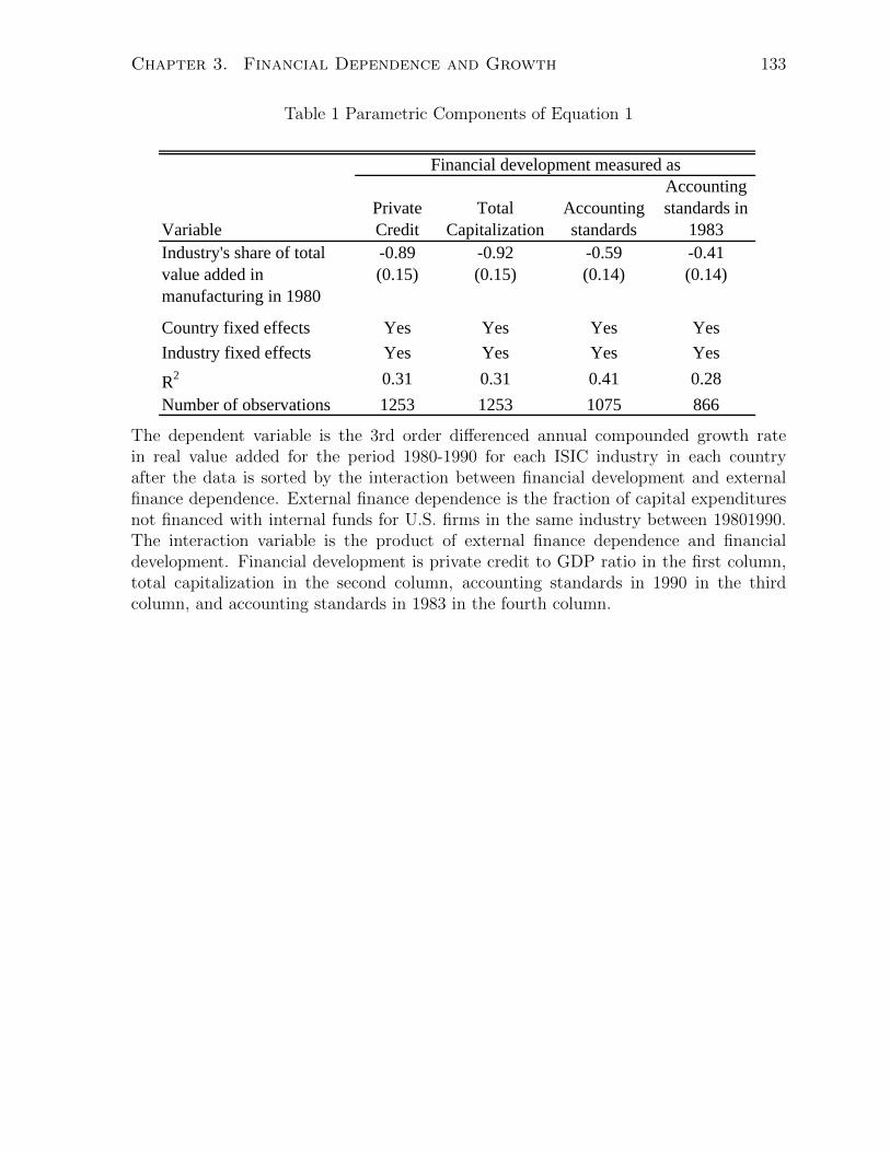
Chapter 3. Financial Dependence and Growth 133
Table 1 Parametric Components of Equation 1
VariablePrivate Credit
Total Capitalization
Accounting standards
Accounting standards in
1983Industry's share of total value added in manufacturing in 1980
-0.89(0.15)
-0.92(0.15)
-0.59(0.14)
-0.41(0.14)
Country fixed effects Yes Yes Yes Yes
Industry fixed effects Yes Yes Yes Yes
R2 0.31 0.31 0.41 0.28
Number of observations 1253 1253 1075 866
Financial development measured as
The dependent variable is the 3rd order differenced annual compounded growth ratein real value added for the period 1980-1990 for each ISIC industry in each countryafter the data is sorted by the interaction between financial development and externalfinance dependence. External finance dependence is the fraction of capital expendituresnot financed with internal funds for U.S. firms in the same industry between 19801990.The interaction variable is the product of external finance dependence and financialdevelopment. Financial development is private credit to GDP ratio in the first column,total capitalization in the second column, accounting standards in 1990 in the thirdcolumn, and accounting standards in 1983 in the fourth column.

Chapter 3. Financial Dependence and Growth 134
Tab
le2
Par
amet
ric
Anal
ogues
ofE
quat
ion
1
Var
iabl
ePr
ivat
e C
redi
tPr
ivat
e C
redi
tTo
tal
Cap
italiz
atio
nTo
tal
Cap
italiz
atio
nA
ccou
ntin
g st
anda
rds
Acc
ount
ing
stan
dard
s
Acc
ount
ing
stan
dard
s in
1983
Acc
ount
ing
stan
dard
s in
1983
Indu
stry
's sh
are
of to
tal
valu
e ad
ded
in
man
ufac
turin
g in
198
0
-0.9
0(0
.14)
-0.9
0(0
.14)
-0.8
7(0
.14)
-0.8
6(0
.14)
-0.4
1(0
.13)
-0.4
4(0
.13)
-0.3
0(.1
3)-0
.31
(0.1
3)
Inte
ract
ion
(ext
erna
l de
pend
ence
x fi
nanc
ial
depe
nden
ce)
0.07
(0.0
2)0.
10(0
.03)
0.06
(.02)
0.10
(0..0
3)0.
14(0
.03)
0.24
(0.0
7)0.
08(.0
4)0.
10(.0
8)
Inte
ract
ion
(ext
erna
l de
pend
ence
x fi
nanc
ial
depe
nden
ce)2
-0.0
2(0
.01)
-0.0
3(0
.02)
-0.0
8(0
.05)
-0.0
2(0
.05)
Cou
ntry
fixe
d ef
fect
sY
esY
esY
esY
esY
esY
esY
esY
esIn
dust
ry fi
xed
effe
cts
Yes
Yes
Yes
Yes
Yes
Yes
Yes
Yes
R2
0.29
0.29
0.28
0.28
0.42
0.42
0.30
0.30
Num
ber o
f obs
erva
tions
1253
1253
1253
1253
1075
1075
866
866
Fina
ncia
l dev
elop
men
t mea
sure
d as
The
dep
enden
tva
riab
leis
the
diff
eren
ced
annual
com
pou
nded
grow
thra
tein
real
valu
ead
ded
for
the
per
iod
1980
-199
0fo
rea
chIS
ICin
dust
ryin
each
countr
y.E
xte
rnal
finan
cedep
enden
ceis
the
frac
tion
ofca
pit
alex
pen
dit
ure
snot
finan
ced
wit
hin
tern
alfu
nds
for
U.S
.firm
sin
the
sam
ein
dust
ryb
etw
een
1980
1990
.T
he
inte
ract
ion
vari
able
isth
epro
duct
ofex
tern
alfinan
cedep
enden
cean
dfinan
cial
dev
elop
men
t.F
inan
cial
dev
elop
men
tis
pri
vate
cred
itto
GD
Pra
tio
inth
efirs
ttw
oco
lum
ns,
tota
lca
pit
aliz
atio
nin
the
thir
dan
dfo
urt
hco
lum
n,
acco
unti
ng
stan
dar
ds
in19
90in
the
fift
han
dsi
xth
colu
mn,
and
acco
unti
ng
stan
dar
ds
in19
83in
the
seve
nth
and
eigh
thco
lum
n.
The
inte
ract
ion
vari
able
isth
epro
duct
ofex
tern
aldep
enden
cean
dfinan
cial
dev
elop
men
t.In
tera
ctio
nte
rmal
one
isth
elinea
rpar
amet
ric
anal
ogue
ofeq
uat
ion
1.In
tera
ctio
nan
din
tera
ctio
nte
rmsq
uar
edar
eth
equad
rati
cpar
amet
ric
anal
ogue
ofeq
uat
ion
1.

Chapter 3. Financial Dependence and Growth 135
Figure 1 Single-equation analysis of averaged growth rates over ten years non-parametriccomponent
Notes: The y-axis is the average annual compounded growth rate in real value added for the period 1980-1990 for
each ISIC industry in each country after differencing with order m=3. External finance dependence is the fraction of
capital expenditures not financed with internal funds by firms in the same industry during the 1980’s. This ratio is set
to 0 if it is negative. Financial development is private credit to GDP ratio. This ratio is positive for all countries. The
negative external finance dependence is set to zero for ease of interpretation. The following picture becomes V-
shaped if negative external finance dependence is not set to zero, with the bottom part of V pointing around 0 and
linear fitted line does not change much. A V-shaped curve still implies that for financially underdeveloped countries,
an improvement in their financial institutions will lead to higher increases in growth rates in industries that are least
dependent on finance. It is also possible to make the fraction of capital expenditures not financed with internal funds
positive by adding the absolute value of the minimum to all values.
ooooooooooooooooooooooooooooooooooooooooooooooooooooooooooooooooooooooooooooooooooooooooooooooooooooooooooooooooooooooooooooooooooooooooooooooooooooooooooooooooooooooooooooooo
o
o
o
oo
ooooo
oooooooooo
ooooooooo
o
ooooo
oooo
o
oo
o
o
ooo
o
o
ooo
oo
o
o
o
o
oooooo
oooo
o
o
ooooooooooooooo
o
oo
ooooooooooooooooooo
ooooooooooo
ooooooo
ooo
o
oooooooooooooooo
o
oooooooooooooooooooooooooooooo
oooooooo
ooooooo
oo
ooo
oooooo
ooooooo
o
ooooooooooooooooooooooo
oooooooooooooooooooo
oooooooo
o
ooo
o
ooooo
o
oooo
o
ooooooooo
o
ooooooooooo
o
o
ooooooooooo
o
ooooo
oo
ooo
o
ooooooooooo
oooo
o
oooooooo
o
ooooooooooooooo
o
o
oooo
o
oooooooooooooooooooooooooooooooooooooo
oo
oooooooooo
oo
o
oo
o
oooooooo
ooo
oooo
o
ooooooooooooo
o
ooooooooooooooooooooo
o
oooooooo
o
ooooooooooooooooooo
o
ooooooooooooooooooooooooooooooo
o
ooooooo
o
oooooooooooooo
o
oooooooooooo
o
ooooo
ooooooooooooooooo
o
o
o
oooooooooo
ooooooooooooooooooooooooooo
o
oo
oo
oooooooooooooooooooooooooooooooooo
o
oooooo
o
oo
o
oooooooo
o
oooooooooooooooooooooooooooooooooooooooooooooo
ooooo
o
ooooo
o
o
o
oooooooooooooooooooooooooooooooooooooo
oo
o
oooooooo
ooooooooo
ooooooooo
o
oo
oooooooooooooo
o
ooooo
ooooooooo
oooooooooooooooooo
ooooooooo
oooo
o
oooooooooooooooooooooooooooooo
o
o
o
o
o
ooo
o
ooooooooooooooooooooooooooooo
o
ooooooo
ooooooooooo
ooo
oooooooooooo
o
ooooooooooo
o
oooooooooooooo
oo
o
ooooooooooooo
oooooo
o
ooooooo
oooo
ooooo
oo
o
ooooo o
ooo
ooo o o
oo o
o o o
Fin Dev*Ext Fin
ind
ustr
y g
row
th
0.0 0.5 1.0 1.5 2.0
-0.5
0.0
0.5
1.0
KernelLinear
The y-axis is the average annual compounded growth rate in real value added for theperiod 1980-1990 for each ISIC industry in each country after differencing with orderm=3. External finance dependence is the fraction of capital expenditures not financedwith internal funds by firms in the same industry during the 1980s. This ratio is setto 0 if it is negative. Financial development is private credit to GDP ratio. This ratiois positive for all countries. The negative external finance dependence is set to zerofor ease of interpretation. The following picture becomes V-shaped if negative externalfinance dependence is not set to zero, with the bottom part of V pointing around 0and linear fitted line does not change much. A V-shaped curve still implies that forfinancially underdeveloped countries, an improvement in their financial institutions willlead to higher increases in growth rates in industries that are least dependent on finance.It is also possible to make the fraction of capital expenditures not financed with internalfunds positive by adding the absolute value of the minimum to all values.

Chapter 3. Financial Dependence and Growth 136
Figure 2 Panel data analysis growth rates 1980-1991 non-parametric component
The y-axis is the average annual compounded growth rate in value added for every fouryears during 1980-1991 for each ISIC industry in each country after differencing withorder m=3. The annual growth rate itself exhibits too much noise and therefore I lookat the panel data in the averages of every four years. The results are similar if I usedthree or five years. External finance dependence is the fraction of capital expendituresnot financed with internal funds by firms in the same industry during the 1980s. Thisratio is set to 0 if it is negative. Financial development is private credit to GDP ratio.This ratio is positive for all countries. The negative external finance dependence is setto zero for ease of interpretation.

Bibliography
Aghion, Philippe, George-Marios Angeletos, Abhijit V. Banerjee, and Kalina Manova.
2010. “Volatility and Growth: Credit Constraints and the Composition of Investment.”
Journal of Monetary Economics 57:246–265.
Aguirregabiria, Victor and Pedro Mira. 2007. “Sequential Estimation of Dynamic Dis-
crete Games.” Econometrica 75 (1):1–54.
Amiti, Mary and David E. Weinstein. 2009. “Exports and Financial Shocks.” Quarterly
Journal of Economics 126 (4):1841–1877.
Antras, Pol. 2003. “Firms, Contracts, and Trade Structure.” Quarterly Journal of
Economics 118 (4):1375–1418.
Antras, Pol, Mihir Desai, and Fritz Foley. 2009. “Multinational Firms, FDI Flows and
Imperfect Capital Markets.” Quarterly Journal of Economics 124 (3):1171–1219.
Antras, Pol and C. Fritz Foley. 2011. “Poultry in Motion: A Study of International Trade
Finance Practices.” NBER Working Paper.
Antras, Pol and Elhanan Helpman. 2004. “Global Sourcing.” Journal of Political Econ-
omy 112 (3):552–580.
Atkeson, Andrew and Ariel Burstein. 2010. “Innovation, Firm Dynamics, and Interna-
tional Trade.” Journal of Political Economy 118 (3):433–484.
137

BIBLIOGRAPHY 138
Auboin, M. 2009. “Boosting the Availability of Trade Finance in the Current Crisis:
Background Analysis for a Substantial G20 Package.” CEPR Working Paper 35.
Aw, Bee Yan, Sukkyun Chung, and Mark J. Roberts. 2000. “Productivity and Turnover
in the Export Market: Micro Evidence from Taiwan (China) and the Republic of
Korea.” World Bank Economic Review 14 (1):65–90.
Aw, Bee Yan, Mark Roberts, and Daniel Xu. 2008. “R&D Investment, Export, and the
Evolution of Firm Productivity.” American Ecnomic Review, Papers and Proceedings
98 (2):451–456.
———. 2011. “R&D Investment,Exporting, and Productivity Dynamics.” American
Ecnomic Review 101 (4):1312–1344.
Aw, Bee Yan, Mark J. Roberts, and Tor Winston. 2007. “Export Market Participation,
Investments in R&D and Worker Training, and the Evolution of Firm Productivity.”
World Economy 14 (1):83–104.
Baldwin, John R. and Wulong Gu. 2003. “Participation in Export Markets and Pro-
ductivity Performance in Canadian Manufacturing.” Canadian Journal of Economics
36 (3):634–657.
Beck, Thorsten. 2002. “Financial Development and International Trade. Is There a
Link?” Journal of International Economics 57 (1):107–131.
———. 2003. “Financial Dependence and International Trade.” Review of International
Economics 11 (2):296–316.
Becker, B. and D. Greenberg. 2005. “Financial Development and International Trade.”
Mimeo, University of Illinois at Urbana-Champain.
Benkard, C. Lanier, Benjamin Van Roy, and Gabriel Y. Weintroub. 2007. “Computational

BIBLIOGRAPHY 139
Methods for Oblivious Equilibrium.” Working Paper No. 9726, National Bureau of
Economic Research,.
———. 2008. “Markov Perfect Industry Dynamics with Many Firms.” Econometrica
76 (6):1375–1411.
Bernard, Andrew B., Jonathan Eaton, Bradford Jensen, and Samuel Kortum. 2003.
“Plants and Productivity in International Trade.” American Economic Review
93 (4):1268–1290.
Bernard, Andrew B. and J. Bradford Jensen. 1999. “Exceptional Exporter Performance:
Cause, Effect, or Both?” Journal of International Economics 47 (1):1–25.
———. 2004. “Exporting and Productivity in the U.S.” Oxford Review of Economic
Policy 20 (3):343–357.
———. 2008. “Reallocation, Firm Turnover and Efficiency: Selection on Productivity or
Profitability?” American Economic Review 98 (1):394–425.
Bernard, Andrew B., Stepehn J. Redding, and Peter K. Schott. forthcoming. “Multi-
product Firms and Trade Liberalization.” American Economic Review .
Bernard, Andrew B. and Joachim Wagner. 1997. “Exports and Success in German
Manufacturing.” Weltwirtschaftliches Archiv 133 (1):134–157.
Blundell, R. and A. Duncan. 1998. “Kernel Regression in Empirical Microeconomics.”
Journal of Human Resources 33:62–87.
Braun, Matias. 2003. “Financial Contractibility and Asset Hardness.” Mimeo, University
of California Los Angeles.
Bustos, Paula. 2011. “Trade Liberalization, Exports, and Technology Upgrading: Ev-
idence on the Impact of MERCOSUR on Argentinian Firms.” American Economic
Review 101 (1):304–340.

BIBLIOGRAPHY 140
Chaney, Thomas. 2005. “Liquidity Constrained Exporters.” Mimeo, University of
Chicago.
Claessens, Stijn and Luc Laeven. 2003. “Financial Development, Property Rights, and
Growth.” Journal of Finance 58 (6):2401–2437.
Clerides, Sofronis, Saul Lach, and James R. Tybout. 1998. “Is Learning by Exporting Im-
portant? Micro-dynamic Evidence from Colombia, Mexico, and Morocco.” Quarterly
Journal of Economics 113 (3):903–947.
Constantini, James A. and Marc J. Melitz. 2008. “The Dynamics of Firm-Level Ad-
justment to Trade.” In The Organization of Firms in a Global Economy, edited by
Elhanan Helpman, Dalia Marin, and Thierry Verdier. Cambridge, MA: Harvard Uni-
versity Press, 107–141.
Das, Sanghamitra, Mark Roberts, and James R. Tybout. 2007. “Market Entry Costs,
Producer Heterogeneity, and Export Dynamics.” Econometrica 75 (3):837–873.
De Loecker, Jan. 2011. “Product Differentiation, Multi-Product firms and Estimating
the Impact of Trade Liberalization on Productivity.” Econometrica 79 (5):1407–1451.
Delgado, Miguel A., Jose C. Farinas, and Sonia Ruano. 2002. “Firm Productivity and
Export Markets: A Non-parametric Approach.” Journal of International Economics
57 (2):397–422.
Dixit, Avinash K. and Joseph E. Stiglitz. 1977. “Monopolistic Competition and Optimum
Product Diversity.” American Economic Review 67 (3):297–308.
Doraszelski, U. and M. Satterhwaite. 2007. “Computable Markov-Perfect Industry Dy-
namics: Existence, Purification, and Multiplicity.” Working Paper, Harvard University.
Ericson, Richard and Ariel Pakes. 1995. “Markov-Perfect Industry Dynamics: A Frame-
work for Empirical Work.” Review of Economic Studies 62:53–82.
BIBLIOGRAPHY 141
Fernandes, Ana M. and Alberto E. Isgut. 2006. “Learning-by-Exporting Effects: Are
They for Real?” Mimeo, The World Bank and Institute for Competitiveness & Pros-
perity.
Hallward-Driemeier, Mary, Giuseppe Iarossi, and Kenneth L. Sokoloff. 2005. “Exports
and Manufacturing Productivity in East Asia: A Comparative Analysis with Firm-
Level Data.” Mimeo, The World Bank and UCLA.
Hart, Oliver D. and John Moore. 1999. “Foundations of Incomplete Contracts.” Review
of Economic Studies 66 (1):115–138.
Hausman, J. 1978. “Specification Tests in Econometrics.” Econometrica 46:1251–1271.
Hopenhayn, Hugo A. 1992. “Entry, Exit and Firm Dynamics in Long Run Equilibrium.”
Econometrica 60 (5):1127–1150.
Hur, Jung, Manoj Raj, and Yohanes Riyanto. 2006. “Finance and Trade: A Cross-
Country Empirical analysis on the Impact of Financial Development and Asset Tan-
gibility on International Trade.” World Development 34 (10):1728–1741.
Lall, Sanjaya. 2000. “The Technological Structure and Performance of Developing Coun-
try Manufactured Exports, 1985-98.” Oxford Development Studies 28 (3):337–369.
Levchenko, Andrei. 2007. “Institutional Quality and International Trade.” Review of
Economic Studies 74 (3):791–819.
Levinsohn, James and Amil Petrin. 2003. “Estimating Production Functions Using Inputs
to Control for Unobservables.” Review of Economic Studies 70 (2):317–342.
Lileeva, Alla. 2004. “Import Competition and Selection.” Working paper, York Univer-
sity,.
BIBLIOGRAPHY 142
Lileeva, Alla and Daniel Trefler. 2010. “Improved Access to Foreign Markets Raises Plant-
Level Productivity... for Some Plants.” Quarterly Journal of Economics 125 (3):1051–
1099.
Manova, Kalina. 2006. “Credit Constraints, Heterogeneous Firms, and International
Trade.” Mimeo, Harvard University.
———. 2008. “Credit Constraints, Equity Market Liberalizations and International
Trade.” Journal of International Economics 76:34–47.
Manova, Kalina and Davin Chor. 2012. “Off the Cliff and Back: Credit Conditions
and International Trade during the Global Financial Crisis.” Journal of International
Economics 87:117–133.
Manova, Kalina, Shang-Jin Wei, and Zhiwei Zhang. 2011. “Firm Exports and Multina-
tional Activity Under Credit Constraints.” NBER.
Maskin, Eric S. and Jean Tirole. 1988. “A Theory of Dynamic Oligopoly, I: Overview
and Quantity Competition with Large Fixed Costs.” Econometrica 56 (3):549–569.
Melitz, Marc J. 2003. “The Impact of Trade on Intra-Industry Reallocations and Aggre-
gate Industry Productivity.” Econometrica 71 (6):1695–1725.
Newey, W., J. Powell, and F. Vella. 1999. “Nonparametric Estimation of Triangular
Simultaneous Equations Models.” Econometrica 67:565–603.
Nunn, Nathan. 2007. “Relationship-Specificity, Incomplete Contracts, and the Pattern
of Trade.” Quarterly Journal of Economics 122 (2):569–600.
Olley, Steven G. and Ariel Pakes. 1996. “The Dynamics of Productivity inthe Telecom-
munications Equipment Industry.” Econometrica 64 (6):1263–1297.
BIBLIOGRAPHY 143
Pakes, Ariel and Paul McGuire. 1995. “Computing Markov-Perfect Nash Equilibria:
Numerical Implications of a Dynamic Differentiated Product Model.” RAND Journal
of Economics 25 (4):555–589.
Park, Albert, Dean Yang, Xinzheng Shi, and Yuan Jiang. 2006. “Exporting and Firm
Performance: Chinese Exporters and the Asian Financial Crisis.” Mimeo, University
of Michigan.
Pavcnik, Nina. 2002. “Trade Liberalization, Exit and Productivity Improvements: Evi-
dence from Chilean Plants.” The Review of Economic Studies 69 (1):245–276.
Porta, Rafael La, Florencio Lopez de Silanes, Andrei Shleifer, and Robert W. Vishny.
1998. “Law and Finance.” Journal of Political Economy 106 (6):1113–1155.
Rajan, Raghuram and Luigi Zingales. 1998. “Financial Dependence and Growth.” Amer-
ican Economic Review 88 (3):559–586.
Rauch, James. 1999. “Networks versus Markets in International Trade.” Journal of
International Economics 48 (1):7–35.
Schmmeiser, Katherine. 2012. “Learning to Export: Export Growth and the Destination
Decision of Firms.” Journal of International Economics 87 (1):89–97.
Schumpeter, J. A. 1911. A Theory of Economic Development. Cambridge, MA: Harvard
University Press.
Sutton, John and Daniel Trefler. 2011. “Deductions from the Export Basket: Capabilities,
Wealth and Trade.” NBER Working Paper 16834.
Svaleryd, Helena and Jonas Vlachos. 2005. “Financial Markets, the Pattern of Indus-
trial Specialization and Comparative Advantage: Evidence from OECD Countries.”
European Economic Review 49:113–144.
BIBLIOGRAPHY 144
Van Biesebroeck, Johannes. 2004. “Exporting Raises Productivity in Sub-Saharan
African Manufacturing Firms.” Journal of International Economics 67 (2):373–391.
Yatchew, Adonis. 1997. “An Elementary Estimator of the Partial Linear Model.” Eco-
nomics Letters 57:1135–1143.
———. 1998. “Nonparametric Regression Techniques in Economics.” Journal of Eco-
nomic Literature 36:669–721.
———. 1999. “Differencing Methods in Nonparametric Regression: Simple Techniques
for the Applied Econometrician.” Manuscript, University of Toronto.
———. 2000. “Scale Economies in Electricity Distribution: A Semiparametric Analysis.”
Journal of Applied Econometrics 15:187–210.