Vertical Integration and Firm Productivity

Hongyi LI∗ Yi LU† Zhigang TAO‡

This version: November 2015

Abstract

This paper uses three cross-industry datasets from China and other

developing countries to study the effect of vertical integration on firm

productivity. Our findings suggest that vertical integration has a neg-

ative impact on productivity, in contrast to recent studies based on

U.S. firms. We argue that in settings with poor corporate governance,

vertical integration reduces firm productivity because it enables inef-

ficient rent-seeking by insiders.

Keywords: Vertical Integration; Firm Productivity; Instrumental

Variable Estimation; Panel Estimation; Rent-Seeking; Corporate Gov-

ernance

JEL Codes: L22, D23, L25

∗UNSW Australia, hongyi@unsw.edu.au†National University of Singapore, ecsluyi@nus.edu.sg‡The University of Hong Kong, ztao@hku.hk

1

1 Introduction

This paper examines the impact of vertical integration on firm productiv-

ity. To do so, we analyze two different cross-industry datasets of Chinese

manufacturing firms and another dataset of firms in developing countries.

We find that firm productivity, as measured by labour productivity, is

negatively correlated with vertical integration in each of our datasets. Taken

together, our results are in contrast to recent empirical findings, largely based

on U.S. data (e.g., Hortacsu and Syverson, 2007; Forbes and Lederman, 2010)

that vertical integration improves firm efficiency. Later in the paper, we pro-

pose a simple explanation for the negative relationship that we observe in

our data: in developing-country settings characterized by poor legal protec-

tions for firms’ investors, vertical integration serves as an inefficient means

for parties in control to extract private benefits.

A number of issues arise when estimating the causal impact of vertical

integration. One concern is a mismeasurement problem: the extent of verti-

cal integration may be mismeasured in conventional (indirect) measures for

vertical integration such as the value-added ratio. A second concern is an

endogeneity problem:1 simple correlations may not capture the true impact

of vertical integration because the vertical integration decision is endogenous

to unobserved factors such as task difficulty. For each of our three datasets,

we take a distinct approach to address these issues.

Our first dataset is based on a 2003 World Bank survey of Chinese manu-

facturing firms. One key feature of this dataset is a direct measure of vertical

integration: the percentage of parts that are produced in-house. This mea-

sure allows us to avoid the mismeasurement problem associated with indirect

measures of vertical integration. Further, we use the degree of local purchase

(a proxy for the extent of site-specificity) as an instrument for vertical in-

tegration. Both OLS and IV estimates indicate that the degree of vertical

integration is negatively correlated with firm productivity.

Our second dataset is based on comprehensive annual surveys of Chinese

industrial firms between 1998 and 2005. Here, we rely on the value-added

ratio as a measure of vertical integration. To control for the fact that the

value-added ratio may potentially vary with the nature of production, we

perform our analysis with a detailed set of 4-digit industry dummies, and then

with firm dummies. To further control for unobserved firm heterogeneity, we

1Gibbons (2005) aptly labels this the ‘Coase-meets-Heckman’ problem.

2

exploit the panel structure of the dataset to study how within-firm variation

in vertical integration over time correlates with firm productivity. We find,

as above, that the degree of vertical integration is negatively correlated with

firm productivity.

Our third dataset draws upon a series of World Bank Enterprise Surveys

in six developing countries (i.e., Brazil, Ecuador, Oman, the Philippines,

South Africa and Zambia) from 2002 to 2006. It contains firm-level sur-

vey information about changes from outsourcing to in-house production of

major production activities. First-difference estimation shows that bringing

major production activities in-house leads to a decrease in firm productivity,

consistent with our findings from the other two datasets.

Our results do not constitute a “smoking gun” for causality. However, our

finding of a negative relationship between vertical integration and firm pro-

ductivity is consistent across datasets and econometric specifications. In par-

ticular, two of our datasets allow for tight empirical identification of within-

firm variation in vertical integration, which is relatively rare in such cross-

industry studies. Taken as a whole, our results provide suggestive evidence of

a general negative relationship from vertical integration to firm productivity

in the developing-country context.

In light of our empirical results, we develop a simple, stylized model

where vertical integration increases firm insiders’ ability to extract private

benefits, and thus strengthens their incentives to engage in expropriatory

activities. Consequently, in poor legal environments where insiders can easily

expropriate, vertical integration has a negative effect on firm productivity.

The model thus provides a potential causal mechanism to explain why vertical

integration may be associated with lower productivity.

On the other hand, when corporate governance is strong and expropria-

tion is difficult, our model predicts that vertical integration improves insiders’

incentives to make productive investments, and thus has a positive effect on

productivity. This model allows us to reconcile existing findings of a positive

relationship between vertical integration and firm productivity in the U.S.

(where investors’ legal protections are strong) and our findings of a nega-

tive relationship in China and other developing economics (where investors’

protections are relatively weak).

This paper is part of a developing literature that studies the relationship

between vertical integration and organizational outcomes.2 In particular, and

2A number of other papers study the impact of vertical integration on market outcomes.

3

in contrast to our results, a number of papers find a positive relationship be-

tween vertical integration and organizational productivity. We discuss these

papers briefly, but first we note a key distinction between these papers and

our analysis: these papers mostly study U.S. firms (and other developed-

country settings), whereas we study China and other developing countries.

We argue in Section 4 that differences in corporate governance between de-

veloping and developed countries may explain the differences between their

results and ours.

Gil (2009) exploits a natural experiment in the Spanish movie industry

to show that vertically integrated distributers make more efficient decisions

about movie run length. Forbes and Lederman (2010), studying U.S. air-

lines, find that vertical integration increases operational efficiency. David,

Rawley, and Polsky (2013), studying U.S. health organizations, show that

integrated organizations exhibit less task misallocation and produce better

health outcomes relative to unintegrated entities. Besides the distinction be-

tween developed- and developing-country settings, these papers focus on a

single industry, whereas our data allow us to draw broader conclusions about

the integration-productivity relationship across manufacturing firms.3

Atalay, Hortacsu, and Syverson (2014) systematically document differ-

ences between integrated and non-integrated U.S. manufacturing plants.4

Perhaps most interestingly, they find that vertical integration is associated

with higher firm productivity, but argue that this relationship is due to a

selection effect (more productive firms happen to be larger, and larger firms

tend to be more vertically integrated), rather than a causal effect of vertical

integration.5 Atalay, Hortacsu, and Syverson (2014) also find that verti-

Chipty (2001) argues that vertical integration results in market foreclosure in the cable

television industry, and that such foreclosure actually improves consumer welfare. Gil

(2015) shows empirically that vertical disintegration results in higher prices for movie

tickets, and attributes this change to a double marginalization effect.3More broadly, limited by data availability, existing studies of the integration-

productivity relationship are generally industry-specific (e.g., Levin, 1981; Mullainathan

and Scharfstein, 2001).4See Hortacsu and Syverson (2007) for a related analysis of cement manufacturing

plants in the U.S.5They write, “ these disparities [between vertically integrated plants and non-integrated

ones] ... primarily reflect persistent differences in plants that are started by or brought

into firms with vertical structures. In other words, while there are some modest changes

in plants’ type measures upon integration, most of the cross sectional differences reflect

selection on pre-existing heterogeneity.”

4

cal ownership structures do not imply substantial production linkages (i.e.

in-house shipments) from upstream divisions to downstream divisions, thus

challenging conventional notions about vertical integration. We skirt this

issue by instead using the proportion of in-house production as a measure of

vertical integration.

The paper proceeds as follows. Data, variables and estimation strategies

are described in Section 2, and empirical findings are presented in Section

3. Section 4 analyzes a simple model of the relationship between vertical

integration and firm productivity. Section 5 concludes.

2 Data Sources and Variables

In this study, we conduct three separate analyses, using three different cross-

industry datasets (i.e., two within-country datasets and one cross-country

dataset). We tailor a distinct econometric strategy for each dataset, based

on the associated data limitations.

The dependent variable in this study is a measure of firm productivity.

Across our three datasets, we focus on labour productivity as a simple, stan-

dard measure of firm performance. Following Hortacsu and Syverson (2007),

we measure labour productivity as the logarithm of output per worker (de-

noted by Labour Productivity). Table 1 presents summary statistics. The

mean and standard deviation of Labour Productivity are 4.322 and 1.562,

respectively, for the first dataset (the SCE), and are 4.917 and 1.193, respec-

tively, for the second dataset (the ASIF).6 The mean and standard deviation

of Change in Labour Productivity for the third dataset (the PESPIC) are

0.154 and 0.799, respectively.

There are two key challenges in investigating the causal impact of vertical

integration. First: in datasets where the vertical integration decision is not

directly observed, conventional proxies may mismeasure the extent of vertical

integration. For example, the value-added ratio is used extensively in the

literature as a measure of vertical integration, but may be sensitive to the

stage of the production process in which a given firm specializes.7

6While both the first and second datasets are about Chinese manufacturing firms, mean

productivity in the ASIF is higher than that in the SCE, presumably because the ASIF

covers non-state-owned enterprises above a certain sales threshold.7Specifically, the value added ratio is generally lower for firms specializing in later stages

of the production process (Holmes, 1999).

5

Second: the degree of vertical integration is endogenous to transaction

difficulty. In particular, Gibbons (2005) argues that integration is compara-

tively advantageous at high-difficulty transactions (which are likely to pro-

duce inefficient outcomes relative to the first-best), and thus that simple

correlations should naively produce a negative relationship between vertical

integration and firm productivity.

The rest of this section describes of each of our three datasets and briefly

summarizes the associated econometric strategy.

Survey of Chinese Enterprises

The Survey of Chinese Enterprises (SCE) was conducted by the World Bank

in cooperation with the Enterprise Survey Organization of China in early

2003. The SCE consists of two questionaires. The first is directed at senior

management, and focuses on enterprise-level information such as market con-

ditions, innovation, marketing, supplier and labour relations, international

trade, finances and taxes, and top management. The second is directed at

the senior accountant and personnel manager, and focuses on ownership, var-

ious financial measures, and labour and training. A total of 18 Chinese cities

were chosen, and 100 or 150 firms from each city were randomly sampled from

the 9 manufacturing industries and 5 service industries.8 In total, 2,400 firms

were surveyed. We focus on the sub-sample of 1,566 manufacturing firms, for

which our instrumental variable for vertical integration can be calculated.

The SCE dataset contains a survey question explicitly designed to mea-

sure the degree of vertical integration: “what is the percentage of parts used

by the firm that are produced in-house (measured by the value of parts)?”

Our measure of vertical integration, Self-Made Input Percentage, is based on

the response to this question. As a direct measure of vertical integration, Self-

Made Input Percentage avoids many of the mismeasurement issues associated

8The 18 cities are: 1) Benxi, Changchun, Dalian and Haerbin in the Northeast; 2)

Hangzhou, Jiangmen, Shenzhen and Wenzhou in the Coastal area; 3) Changsha, Nan-

chang, Wuhan and Zhengzhou in Central China; 4) Chongqing, Guiyang, Kunming and

Nanning in the Southwest; 5) Lanzhou and Xi’an in the Northwest. The 14 industries are:

1) manufacturing: garment and leather products, electronic equipment, electronic parts

making, household electronics, auto and auto parts, food processing, chemical products

and medicine, biotech products and Chinese medicine, and metallurgical products; and

2) services: transportation services, information technology, accounting and non-banking

financial services, advertising and marketing, and business services.

6

with the conventional alternatives.9 However, this measure is self-reported

and subjective: managers at different companies may have a different under-

standing of what constitutes an input, or how to enumerate parts. In fact,

Self-Made Input Percentage is reported to be 100% for some firms and zero

for others, resulting in substantial amounts of noise: the variable has a mean

value of 0.339 and a standard deviation of 0.401. Consequently, industry

dummies are included in the regression analysis; this mitigates the subjec-

tivity problem because amongst firms in the same industry, managers have a

more or less common understanding of what constitutes parts used in their

production activities.10

Because our variation in Self-Made Input Percentage is cross-sectional,

endogeneity problems may arise from unobserved permanent firm-level het-

erogeneity. In response, we instrument for Self-Made Input Percentage using

Local Purchase: the ratio of inputs purchased from the province where the

firm is located to all purchased inputs. The argument underlying this choice

is that firms with higher site-specificity (as measured by Local Purchase)

vis-a-vis their suppliers are more vulnerable to hold-up,11 which leads to a

9We consulted with the designer of the SCE, who explained that the rationale for

including a survey question on the degree of vertical integration was precisely because of

the well-known problems associated with the conventional measure of vertical integration.10The actual survey was carried out by the Enterprise Survey Organization of China’s

National Bureau of Statistics – an authoritative and experienced survey organization.

Further, as far as we are aware, the survey participants did not raise any issues about

potential ambiguity of the question on vertical integration.11Site specificity could go hand in hand with asset specificity. For example, an electricity-

generating plant located next to a coal mine may adjust its production technology to suit

the quality of locally-obtained coal, which may lead to severe holdup problems ex-post.

Nonetheless, we control for input specificity in one of our robustness checks and find similar

results.

Moreover, even in the absence of asset specificity, monopolistic suppliers may hold up

their nearby customers by demanding higher prices because such customers would have

to pay higher transport costs if purchasing from alternative and more distant suppliers.

Indeed, BHP and Rio Tinto of Australia demanded extra price increases for iron ore pur-

chased by Chinese steel makers in 2005 and 2008 respectively, simply because they are

geographically closer to China than is CVRD of Brazil, despite the same free-on-board

prices of iron ore applying (Png, Ramon-Berjano, and Tao, 2006, 2009). Subsequently,

many Chinese steel makers have been trying to acquire iron ore mines in Australia. Mean-

while, within China, due to high transport costs and local protectionism, both of which

inhibit cross-regional trade, firms have limited options other than purchasing locally, which

further exacerbates the holdup problems associated with local purchases.

7

higher degree of vertical integration; see, e.g., Williamson (1983, 1985).12

Annual Survey of Industrial Firms

The Annual Survey of Industrial Firms (ASIF) was conducted by the Na-

tional Bureau of Statistics of China during the 1998–2005 period. This is

the most comprehensive firm-level dataset in China; it covers all state-owned

and non-state-owned industrial enterprises with annual sales of at least five

million Renminbi.13 The number of firms varies from over 140,000 in the

late 1990s to over 243,000 in 2005. This panel dataset allows us to exploit

within-firm time-series variation in the degree of vertical integration, thus

eliminating any potential endogeneity problems due to permanent firm het-

erogeneity.

The ASIF consists of standard accounting information on firms’ opera-

tions and performance. Our analysis of the ASIF dataset thus relies on the

conventional, albeit objective, measure of vertical integration: Value-Added

Ratio. This variable has a mean value of 0.244 and a standard deviation of

0.164. To mitigate mismeasurement issues, we control for a full set of 4-digit

industry dummies.

Private Enterprise Survey of Productivity and the In-

vestment Climate

The Private Enterprise Survey of Productivity and the Investment Climate

(PESPIC) is a standardized cross-sectional firm-level dataset based on World

Bank Enterprise Surveys (WBESs) conducted by the World Bank’s Enter-

prise Analysis Unit in 68 developing economies during the 2002–2006 pe-

riod.14 The PESPIC’s structure is similar to that of the SCE. The first part

is a general questionaire directed at senior management, focusing on firm

structure and performance, sales and suppliers, investment and infrastruc-

ture, government relations, innovation, and labour relations. The second

part is directed at the senior accountant, and focuses on various financial

measures.

12This theoretical prediction has been supported empirically, e.g., by Masten (1984),

Joskow (1985), Spiller (1985), and Gonzalez-Daz, Arrunada, and Fernandez (2000).13As of July 2015, the exchange rate was approximately 1 Renminbi to 0.15 U.S. dollars.14More information about the dataset can be found at

http://www.enterprisesurveys.org/

8

Although the PESPIC is cross-sectional, it also has some time-series as-

pects. Importantly, this dataset contains a survey question designed to di-

rectly measure changes in the degree of vertical integration: “Has your com-

pany brought in-house major production activities in the last three years?”

The reply to this survey question is used to construct a dummy variable,

Change in Vertical Integration, which equals 1 if the firm answers yes and

0 otherwise. The PESPIC thus allows us to exploit within-firm variation in

the degree of vertical integration and avoid endogeneity problems that might

arise from firm-level heterogeneity. As with the SCE, the PESPIC’s measure

of vertical integration is direct and less prone to potential mismeasurement

problems. Further, by focusing only on “major production activities”, the

PESPIC measure is arguably less prone to subjective interpretation by man-

agers than the corresponding SCE measure.

As the PESPIC was compiled from a series of WBESs employing differ-

ent questionnaire designs and survey methodologies in different countries,

information about the change in the sourcing strategy adopted for major

production activities is available in only 6 countries (i.e., Brazil, Ecuador,

Oman, the Philippines, South Africa and Zambia). After deleting observa-

tions missing valid information about vertical integration choices, we have a

final sample of 3,958 firms in these 6 developing countries. The mean value of

Change in Vertical Integration is 0.097 and the standard deviation is 0.296.

3 Empirical Analysis

This section presents details of our econometric specifications and results.

We devote one subsection to each of the three datasets.

3.1 Survey of Chinese Enterprises: Results

Benchmark Results: OLS To investigate the relationship between ver-

tical integration and firm productivity in the cross-sectional SCE dataset, we

estimate the following equation:

Yf = α + β · V If +X ′ficγ + εf (1)

where f , i, c denote firm, industry and city, respectively; Yf is firm f ’s

productivity; V If is firm f ’s degree of vertical integration (specifically, Self-

Made Input Percentage, constructed on the basis of firm f ’s reply to the

9

survey question “what is the percentage of parts used by the firm that are

produced in-house (measured by the value of parts)?”); X ′fic is a vector of

control variables including firm characteristics,15 CEO characteristics,16 city

dummies and industry dummies; and εf is the error term. Standard errors are

clustered at the industry-city level to correct for potential heteroskadasticity.

The OLS regression results for various specifications of equation (1) are

reported in Table 2. For all specifications, the estimated coefficients of Self-

Made Input Percentage are consistently negative and statistically significant:

a higher degree of vertical integration is associated with lower firm produc-

tivity. Taking the most conservative estimate, a one-standard-deviation in-

crease in the degree of vertical integration leads to a 2.2% decrease in firm

productivity at the mean level.

Note that the regressions produce reasonable estimates for the effects of

control variables. For example, younger firms and those with higher capital

intensity have higher productivity, consistent with findings in the literature.

Firms with a higher percentage of private ownership also have higher produc-

tivity. This is consistent with the observation that state-owned enterprises

in China are charged with multiple mandates: they are required to focus

not only on profit maximization, but also on maintaining social stability, the

latter of which involves excessive hiring and consequently lower productivity

(Bai, Li, Tao, and Wang, 2000). The coefficient on Firm Size is positive and

significant in all specifications, suggesting the presence of economies of scale.

This is consistent with evidence of local protectionism within China (Young,

2000; Bai, Du, Tao, and Tong, 2004), which results in production at a sub-

optimal scale. Finally, government appointments have a negative impact on

firm productivity. This result is consistent with the view that government

15Variables related to firm characteristics include: Firm Size (measured as the logarithm

of firm employment), Firm Age (measured as the logarithm of years of establishment),

Percentage of Private Ownership (measured as the percentage of equity owned by parties

other than government agencies) and Capital Intensity (measured as the logarithm of

assets per worker).16The CEO characteristics include measures of human capital – Education (years of

schooling), Years of Being CEO (years as CEO) and Deputy CEO Previously (an indi-

cator of whether the CEO had been the deputy CEO of the same firm before becoming

CEO); and measures of political capital – Government Cadre Previously (an indicator of

whether the CEO had previously been a government official), Communist Party Mem-

ber (an indicator of whether the CEO is a member of the Chinese Communist Party)

and Government Appointment (an indicator of whether the CEO was appointed by the

government).

10

appointments of CEOs in China are based on political considerations rather

than managerial talent.

IV Estimates Because our variation in Self-Made Input Percentage is

cross-sectional, endogeneity problems may arise from unobserved permanent

firm-level heterogeneity. We thus instrument for Self-Made Input Percent-

age using Local Purchase. The IV estimation results are presented in Table

3. Only the industry dummy is included in Column 1, whereas all control

variables are included in Column 2. The IV estimate of Self-Made Input

Percentage remains negative and statistically significant. In fact, the IV es-

timates are substantially larger than the OLS estimates. One possibility is

that the self-reported degree of vertical integration involves some measure-

ment errors, which biases the OLS estimates downward (towards zero).

As shown in Panel B, Local Purchase is found to be positive and sta-

tistically significant. The Anderson canonical correlation LR statistic and

the Cragg-Donald Wald statistic (reported in Panel C) further confirm that

our instrument is relevant. The F-test of excluded instrument is statistically

significant at the 5% level, but has a value of around 5, which is below the

critical value of 10 – a value suggested by Staiger and Stock (1997) as the

“safety zone” for a strong instrument. This raises possible concerns of a weak

instrument for our analysis. In response, we conduct two additional tests:

the Anderson-Rubin Wald test and the Stock-Wright LM S-statistic, which

offer reliable statistical inferences under a weak instrument setting (Anderson

and Rubin, 1949; Stock and Wright, 2000). Both tests produce statistically

significant results, implying that our main results are robust to the presence

of a weak instrument.

Instrument Validity Our instrumental variable estimation should satisfy

the exclusion restriction: the instrument Local Purchase should not affect

firm productivity through channels other than the degree of vertical inte-

gration. Note that our instrumental variable estimation includes industry

dummies to control for omitted-variable bias due to technological differences

across industries, as well as city dummies to control for any locational ad-

vantages that may simultaneously affect local purchases, vertical integration

and firm productivity. In addition to these controls, we conduct two sets of

robustness checks on the exclusion restriction.

First, we identify four possible channels other than vertical integration

11

through which the instrument may affect firm productivity and then explic-

itly control for these channels in the IV estimation. First, when a firm sources

more of its parts and components locally, it may incur lower transportation

costs, which subsequently leads to higher firm productivity. Second, the

shorter distance to suppliers under local sourcing implies lower inventory re-

quirements, leading to higher productivity. Third, locally purchased inputs

may be made to firms’ unique specifications, which adds more value to their

final products. Fourth, local purchases could reduce delays in delivery and

consequently minimize lost sales.

From the SCE dataset, we construct four variables corresponding to each

of these four possible alternative channels: Transportation Cost (measured

by transportation costs divided by sales), Inventory (measured by inventory

stocks of final goods over sales), Input Specificity (measured by the percent-

age of a firm’s inputs made to the firm’s unique specifications) and Delivery

Loss (measured by the percentage of sales lost due to delivery delays in the

previous year). We include linear and quadratic terms for each of these chan-

nel variables in the IV estimation. As shown in Columns 1 – 5 of Table 4, our

main results regarding the impact of vertical integration on firm productivity

remain robust to these additional controls for potential alternative channels.

Further Robustness Checks Our results could potentially be driven by

a few outlying observations. To address this concern, we exclude the top

and bottom 1% of observations by firm productivity and repeat the analysis

using both OLS and IV regression methods. As shown in columns 1 and 2

of Table 5, our main results regarding the impact of vertical integration on

firm productivity remain robust to these exercises.

We then carry out the analysis using two sub-samples. First: for firms

with many businesses, the degree of vertical integration could vary from one

business to another. Thus, our measure of vertical integration may reflect the

average degree of vertical integration across various businesses, which may

bias our estimations of the impact of vertical integration on firm productivity.

To address this concern, we restrict attention to the sub-sample of firms with

focused business (defined as firms whose main business accounts for more

than 50% of total sales); these results are reported in Columns 3 and 4 of

Table 5. Second: China’s state-owned enterprises, as legacies of its central

planning system, are burdened with social responsibility mandates, and thus

tend to be vertically integrated and inefficient. To check that our results are

12

not driven by these state-owned enterprises, we focus on the sub-sample of

private firms; these results are reported in Columns 5 and 6 of Table 5. Our

finding that vertical integration and firm productivity are negatively related

continues to hold in both sub-samples.

3.2 Annual Survey of Industrial Firms: Results

Panel Analysis We now turn to the Annual Survey of Industrial Firms

(ASIF). As the ASIF is a panel dataset, we use the following regression

specification:

Yf,t = αf + β · V If,t + γt + εf,t, (2)

where Yf,t is the productivity of firm f in year t; V If,t is the value added ratio

of firm f in year t, measuring the degree of vertical integration; αf is the firm

dummy, capturing all time-invariant firm characteristics; and γt is the year

dummy, capturing all the effects affecting firms in year t. Standard errors

are clustered at the firm-level to deal with the potential heteroskadasticity

problem.

As an initial benchmark, pooled OLS estimation results are reported in

Column 1 of Table 6. There, we replace the firm dummy αf in Equation 2

with a full set of 4-digit industry and province dummies. We find that Value

Added Ratio has a negative and statistically significant estimated coefficient,

consistent with our findings obtained using the SCE dataset.

Returning to Equation 2, panel fixed effect estimation results are reported

in Column 2 of Table 6. The estimated coefficient of Value Added Ratio is

still negative and statistically significant: a within-firm increase in vertical

integration is associated with a decrease in firm productivity. Note, how-

ever, that the magnitude of the estimated coefficient falls from -1.274 to

-0.627 when we move from pooled OLS to panel fixed-effects. This drop in

magnitude could be attributed to the control for time-invariant firm-level

unobserved characteristics (e.g., the level of transaction difficulty) correlated

with both the degree of vertical integration and firm productivity. It is also

possible that some variations in the degree of vertical integration occur at

the inter-firm rather than the intra-firm level, as a result of which intra-firm

variations have a muted impact on firm productivity in the panel fixed effect

estimation.

While we have controlled for all time-invariant firm-level unobservables

through the panel fixed-effect estimation, time-varying omitted variable bias

13

remains a concern. Proxying for time-varying omitted variables using the

lagged dependent variable (Wooldridge, 2002), we estimate the following

equation:

Yf,t = αf + β · V If,t + δ · Yf,t−1 + γt + εf,t. (3)

The estimation results are reported in Column 3 of Table 6. After controlling

for time-varying unobservables, the impact of vertical integration on firm

productivity remains negative and statistically significant.

Further, with the inclusion of the lagged dependent variable in the panel

estimation, dynamic estimation bias – whereby the lagged dependent variable

is correlated with the error term – may arise, leading to biased estimates. To

address this concern, we conduct a panel instrumental-variable estimation a

la Anderson and Hsiao (1982). More specifically, in the First-Difference trans-

formation of equation (3), we instrument ∆V If,t and ∆Yf,t−1 with V If,t−1and Yf,t−2, respectively. The Anderson-Hsiao IV estimation results are re-

ported in Column 4 of Table 6. Our main finding that vertical integration

has a negative impact on firm productivity continues to hold here.

Robustness Checks First, to address the concern that firm entry and exit

during the sample period may drive our findings, we restrict our analysis to

a balanced panel, comprising firms present for the whole sample period. The

panel fixed-effect and Anderson-Hsiao IV estimation results are reported in

Columns 1-2 of Table 7. Our main finding continues to hold in this balanced

sub-sample.

Second, we exclude the top and bottom 1% of observations for firm pro-

ductivity to check whether our results are mainly driven by outlying obser-

vations. The panel fixed-effect and Anderson-Hsiao IV estimation results are

reported in Columns 3-4 of Table 7. Our main finding continues to hold after

excluding outliers.

Third, in the context of China, one may be concerned that our results

are driven by state-owned enterprises, which are usually less productive but

highly integrated. To address this concern, we restrict our analysis to the

sub-sample of private firms. The panel fixed-effect and Anderson-Hsiao IV

estimation results are reported in Columns 5-6 of Table 7. Our main finding

continues to hold in the sub-sample of private firms.

Fourth, to account for the within-industry firm heterogeneity in techno-

logical capability (which could in turn affect firm productivity and ownership

structure), we include Capital Intensity (measured as the logarithm of assets

14

per worker) as an additional control. The panel fixed-effect and Anderson-

Hsiao IV estimation results are reported in Columns 7-8 of Table 7. Our

main finding is robust to this additional control.

3.3 PESPIC: Results

First-Difference Estimation The key independent variable in our anal-

ysis of the cross-country PESPIC dataset is Change in Vertical Integration,

which provides a source of within-firm variation in vertical integration. We

estimate the following First-Difference equation:

∆Yf,t = α + β ·∆V If,t +X′

f,t−3γ + ∆εf,t, (4)

in which ∆Yf,t is the change in firm productivity, ∆V If,t is the change in the

degree of vertical integration for major production activities, and X′

f,t−3 is

a vector of firm-level variables (Initial Firm Size and Initial Sales Change,

reflecting firm size and year-on-year sales growth at time t − 3). Standard

errors are clustered at the firm-level.

First-Difference estimation results of equation (4) are reported in Column

1 of Table 8. The coefficient of the Change in Vertical Integration is nega-

tive and statistically significant, suggesting that bringing major production

activities in-house leads to a decrease in firm productivity.

While First-Difference estimation allows us to effectively control for all

time-invariant characteristics, there could still be some time-varying charac-

teristics correlated with the change in vertical integration, which would then

lead to biased estimates. To address this concern, we include several mea-

sures of important operational changes in the past three years as robustness

checks.

The PESPIC dataset contains the following questions: (1) “Has your

company introduced any new technology that has substantially changed the

way that the main product is produced in the last three years?”; (2) “Has

your company agreed any new joint venture with a foreign partner in the last

three years?”; (3) “Has your company obtained any new licensing agreement

in the last three years?”; and (4) “Has your company developed any major

new product line in the last three years?”. Accordingly, we construct four

control variables – Introduction of New Technology, Introduction of New Joint

Venture, Introduction of New Licensing Agreement, and Introduction of New

Major Product Line – each of which takes the value of 1 if the firm replies

15

affirmatively to the respective question and 0 otherwise. In addition, we

construct a variable related to the change in capital intensity (i.e., measured

as the change in logarithm of assets per worker) to control for possible within-

industry heterogeneity in technologies.

We include these five additional control variables in the model in a step-

wise manner in Columns 2-6 of Table 8. Our regressor of interest, Change in

Vertical Integration, continues to produce a negative and statistically signif-

icant impact on firm productivity, implying the robustness of our findings in

Column 1 to possible time-varying characteristics.

Robustness Checks We conduct two further robustness checks on our

PESPIC analysis. First, to address the possibility that our results could be

driven by outliers, we exclude the top and bottom 1% of observations for

firm productivity and repeat the analysis. As shown in Column 1 of Table

9, our main finding remains robust to this exercise.

Second, casual observations suggest that state-owned enterprises in de-

veloping countries tend to be inefficient, yet they shoulder their social re-

sponsibilities by becoming more vertically integrated, which may explain the

negative impact of vertical integration on firm productivity. To ensure that

our results are not driven by the presence of state-owned enterprises, we fo-

cus on a sub-sample of private firms. As shown in Column 2 of Table 9, our

main finding continues to hold in this sub-sample.

3.4 Discussion

There are tradeoffs involved in each of our datasets. The SCE dataset in-

cludes a direct measure of vertical integration (the independent variable), but

cross-sectional regressions may suffer from endogeneity problems due to un-

observed firm-level heterogeneity. Our analysis utilizes a plausible instrument

for vertical integration; controls for a large set of variables including industry

dummies, city dummies and CEO and firm characteristics; and conducts a

number of robustness checks. Nonetheless, we cannot exclude the possibility

that the exclusion restriction is violated to some degree by our instrument.

The ASIF and PESPIC datasets allow us to conduct panel analyses that

exploit within-firm variation in vertical integration over time. This allows

us to control for any endogeneity problems arising from permanent firm het-

erogeneity. That said, we cannot completely eliminate potential firm-specific

16

time-varying shocks that drive both vertical integration decisions and firm

productivity, although we do include a host of relevant controls for the PE-

SPIC dataset. That ASIF dataset also relies on Value Added as a measure of

vertical integration, which may be susceptible to mismeasurement problems;

this issue is partially alleviated by our inclusion of a detailed set of 4-digit

industry dummies (and, in some specifications, firm dummies). On the other

hand, the PESPIC analysis utilizes a direct (albeit potentially subjective)

measure of vertical integration.

Despite the limitations of each dataset, our overall analysis paints a pic-

ture of a significant negative relationship between vertical integration and

firm productivity that is robust to various specifications and measures of ver-

tical integration, and holds in a variety of cross-industry developing-country

contexts. This suggests that there might be robust economic mechanisms

leading to such a negative relationship; we discuss one potential mechanism

in Section 4.

4 A Simple Model: Vertical Integration, Rent-

Seeking, and Firm Performance

This section presents a simple and very stylised model of vertical integration.

In the model, integration corresponds to firm insiders (e.g. firm manage-

ment) retaining key decision-rights that determine the outcome of produc-

tion, whereas outsourcing corresponds to the (partial) transfer of decision

rights to outside suppliers.

As a quick preview: the key source of inefficiency in the model is that inte-

gration gives insiders more control over the production process, and thus en-

ables their rent-seeking activities. Outsourcing, by reducing insider control,

reduces incentives for such rent-seeking because the returns to rent-seeking

have to be shared between insider and supplier. The dark side of outsourcing

is that it also suppresses insiders’ incentives for productive investments.

There is a single insider (who we may think of as an entrenched man-

ager, or the firm’s majority shareholder), and a unit mass of infinitesimally-

weighted tasks to be performed. Mass m ∈ (0, 1) of tasks are integrated (i.e.

the insider performs the task), and the remaining 1−m tasks are outsourced

(an outside supplier performs the task). Outside suppliers are specialized,

so each supplier can perform a maximum of one (infinitesimal) task for the

17

firm. Each task θ produces revenue πθ. Firm revenue is simply the integral

of revenue across all tasks:

π =

∫ 1

0

πθdθ. (5)

For each task θ, the player performing the task chooses two investments:

a productive investment iθ ≥ 0 and a rent-seeking activity jθ ≥ 0, incurring

private cost cθ = 12i2θ + 1

2αj2θ . Parameter α represents the ease of expropri-

ation: higher α represents weaker legal protections which allow the player

performing the task to expropriate from the firm more easily.

The investments iθ and jθ have to be implemented, which requires the

cooperation of the manager; the underlying premise is that insourcing of task

θ corresponds to the insider having “sole control” over θ, whereas outsourcing

corresponds to “joint control” by insider and supplier.17

If implemented, the productive investment increases firm revenue, whereas

the rent-seeking investment increases the player’s private benefit vθ at the

expense of revenue:

πθ = iθ − jθ, (6)

vθ = jθ. (7)

For each task θ, revenue πθ and private benefits vθ are not contractible,

so formal incentive contracts cannot be offered to outside suppliers.18 The

insider receives fraction b ∈ (0, 1) of total revenue π; note that she is not a

residual claimant.19

The overall timing of the model is as follows:

1. For each task θ being outsourced, the insider makes the outside supplier

a participation offer κθ. If the supplier accepts, then he receives κθ

17We may alternatively assume that if activity θ is outsourced, then the supplier has

sole control and appropriates all surplus from his investments. This assumption would

produce similar results.18We may allow for a verifiable, noisy signal of firm revenue y = π + ε to be available.

However, because each task is infinitesimal, firm revenue would be uncorrelated with

revenue from each task, and thus incentive contracts for suppliers based on firm revenue

would be ineffective. The premise is that because there are many suppliers who each

make only a small contribution to firm revenue, incentive provision based on firm revenue

becomes prohibitively costly, especially in the presence of contracting frictions such as

supplier risk-aversion.19Think of the remaining share of revenue as going to passive shareholders who have no

say in firm decision-making.

18

from the insider; otherwise the task is not performed, and the supplier

receives zero utility.

2a. For each task θ being performed, the player performing the task chooses

iθ and jθ.

2b. For each task θ being outsourced (and performed), the insider and sup-

plier bargain over whether to implement the investment. If bargaining

fails, then the outcome is zero value-added and zero private benefits:

πθ = 0 and vθ = 0. We impose efficient Nash bargaining, so insider and

supplier split the bargaining surplus equally. (Under integration, the

manager appropriates all the bargaining surplus.)

Total surplus, computed over all tasks, is total revenue plus total private

benefits, less private costs:

surplus =

∫ 1

0

(πθ + vθ − cθ) dθ.

4.1 Integration versus Outsourcing

Lemma 1. Suppose task θ is integrated. Then the manager chooses i∗θ = b

and j∗θ = (1− b)α. Revenue from the task is i− j = b− (1− b)α.

Proof. Under insourcing, the insider chooses iθ and jθ to maximize his payoff

b(iθ− jθ) + jθ− 12i2θ − 1

2αj2θ , i.e. i∗θ = b and j∗θ = (1− b)α. Net revenue for the

task is then i− j = b− (1− b)α.

Under integration, as the fraction b of revenue that the insider receives

increases, he decreases his rent-seeking investment (which increases private

benefits but at the expense of revenue). Also, the insider’s rent-seeking

investments are increasing in the ease of expropriation α. On the other

hand, as b increases, the insider increases his productive investment.

Lemma 2. Suppose task θ is outsourced. Then the supplier for that task

chooses i∗θ = b/2 and j∗θ = (1−b)α2

. Revenue from the task is i− j = b2− 1−b

2α.

Proof. The supplier’s disagreement payoff is κθ− 12i2θ− 1

2αj2θ , while the insider’s

disagreement payoff is −κθ. On the other hand, the total payoff (insider

plus supplier) following implementation is b(iθ − jθ) + jθ − 12i2θ − 1

2αj2θ . The

19

bargaining surplus is thus b iθ + (1 − b)jθ, and the supplier’s net payoff is

κθ + b2iθ + 1−b

2jθ − 1

2i2θ − 1

2αj2θ . To maximize his payoff, the supplier chooses

i∗θ = b2

and j∗θ = (1−b)α2

. Revenue from task θ is thus i− j = b2− 1−b

2α.

Compared to the insider’s choices under integration, the (supplier’s) pro-

ductive investment and rent-seeking investments under outsourcing are each

halved. Under outsourcing, the supplier has to share the returns from his

productive and rent-seeking investments with the insider; thus his incentives

for both investments are suppressed relative to the insider’s incentives under

integration, where the insider keeps the “full” returns from his investments.

The tradeoff between integration and outsourcing is thus as follows: in-

tegration increases productive investments, but also results in more costly

rent-seeking. Importantly, an increase in the ease of expropriation α in-

creases the extent of rent-seeking, and consequently makes outsourcing more

profitable relative to integration.

Proposition 1. Firm revenue is

π =1− b

2

(b

1− b− α

)(1 +m) ,

which is decreasing in the extent of integration m if α > b1−b , and increasing

in m otherwise.

Proof. From Lemmas 1 and 2, integrated tasks contribute b − (1 − b)α of

revenue per unit mass, whereas outsourced tasks contribute b2− 1−b

2α of

revenue per unit mass. Mass m of tasks are integrated and mass 1 −m are

outsourced, so firm revenue is

π = m (b− (1− b)α) + (1−m) (b/2− (1− b)α/2)

= (1− b) (b/(1− b)− α) (1 +m) /2.

Thus integration is more profitable than outsourcing if and only if the

ease of expropriation α is large.20

20Similarly, we may show that total surplus (revenue plus managerial and supplier

payoffs) is increasing in the degree of integration if and only if α is small, i.e., ex-

propriation is difficult. Each task θ produces surplus iθ − i2θ/2 − j2θ/(2α). In particu-

lar, integrated tasks produce b − b2

2 −(1−b)2α

2 of surplus per unit mass, and outsourced

tasks produce b2 −

b2

8 −(1−b)2α

8 of surplus per unit mass. Consequently, total surplus is

m(b− b2

2 −(1−b)2α

2

)+ (1 −m)

(b2 −

b2

8 −(1−b)2α

8

), which is increasing in m if and only

if α < 43b(1−3b/4)(1−b)2 .

20

In other words: the effect of an increase in the degree of firm integration

on revenue depends on the quality of the legal environment. In good (bad)

legal environments where expropriation is difficult (easy), an increase in firm

integration results in an increase (decrease) in firm revenue. In particular, the

case of high α matches our setting of China and other developing countries,

where legal protections are relatively weak and expropriation is easy. In that

case, Proposition 1 predicts that firm productivity (as measured by revenue)

is decreasing in the degree of vertical integration. This matches the empirical

findings from Section 3.

4.2 Discussion

Our model exogenously specifies the degree m of firm integration. We do

not take a stand on the source of variation in the integration decision across

firms. One potential source of variation is managerial capability: more capa-

ble insiders can handle more integrated tasks without relying on suppliers,

and thus choose a greater degree of integration for the firms they manage.21

Under this interpretation, our model suggests that in poor legal environ-

ments, competent managers actually decrease welfare, because they apply

their capabilities towards rent-seeking rather than productive activities.

5 Conclusion

This paper investigates the impact of vertical integration on firm productiv-

ity. This line of research is fraught with mismeasurement and endogeneity

problems; our approach is to analyze, separately, three different datasets that

address the mismeasurement and endogeneity problems in different ways.

Throughout our analysis, we consistently find that the degree of vertical in-

tegration has a negative and statistically significant impact on firm produc-

tivity. This consistency, as well as the cross-industry nature of our samples,

suggests that our findings may be quite broadly applicable, with the following

21Similarly, we take the share b of insider’s revenue as exogenous; this could represent

the shareholdings of a controlling shareholder, or the incentive scheme offered to the CEO.

Under the premise that insiders’ capability varies across firms, our implicit assumption

is that the insider’s managerial capability is private information, and that sophisticated

mechanisms to elicit this private information are unavailable / infeasible; consequently, m

and b cannot be conditioned on managerial capability.

21

caveat.

Our results (based on Chinese and other developing-country firms) con-

trast with recent empirical findings (largely based on U.S. firms) that vertical

integration is positively correlated with firm productivity. We propose that

the differences between their results and ours are driven by differences in the

ease of rent-seeking in developed versus developing countries. In particular,

weak legal environments complement integrated firm structures in enabling

rent-seeking by firm insiders, so the costs of integration are exacerbated in

developing countries where legal protections are weak.

22

References

Anderson, T. W., and C. Hsiao (1982): “Formulation and estimation of

dynamic models using panel data,” Journal of Econometrics, 18(1), 47–82.

Anderson, T. W., and H. Rubin (1949): “Estimation of the Parameters

of a Single Equation in a Complete System of Stochastic Equations,” The

Annals of Mathematical Statistics, 20(1), 46–63.

Atalay, E., A. Hortacsu, and C. Syverson (2014): “Vertical Integra-

tion and Input Flows,” The American Economic Review, 104(4), 1120–

1148.

Bai, C.-E., Y. Du, Z. Tao, and S. Y. Tong (2004): “Local protectionism

and regional specialization: evidence from China’s industries,” Journal of

International Economics, 63(2), 397–417.

Bai, C.-E., D. D. Li, Z. Tao, and Y. Wang (2000): “A Multitask

Theory of State Enterprise Reform,” Journal of Comparative Economics,

28(4), 716–738.

Chipty, T. (2001): “Vertical Integration, Market Foreclosure, and Con-

sumer Welfare in the Cable Television Industry,” The American Economic

Review, 91(3), 428–453.

David, G., E. Rawley, and D. Polsky (2013): “Integration and Task

Allocation: Evidence from Patient Care,” Journal of Economics & Man-

agement Strategy, 22(3), 617–639.

Forbes, S. J., and M. Lederman (2010): “Does vertical integration af-

fect firm performance? Evidence from the airline industry,” The RAND

Journal of Economics, 41(4), 765–790.

Gibbons, R. (2005): “Four formal(izable) theories of the firm?,” Journal of

Economic Behavior & Organization, 58(2), 200–245.

Gil, R. (2009): “Revenue Sharing Distortions and Vertical Integration in

the Movie Industry,” Journal of Law, Economics, and Organization, 25(2),

579–610.

23

(2015): “Does Vertical Integration Decrease Prices? Evidence from

the Paramount Antitrust Case of 1948,” American Economic Journal:

Economic Policy, 7(2), 162–191.

Gonzalez-Daz, M., B. Arrunada, and A. Fernandez (2000): “Causes

of subcontracting: evidence from panel data on construction firms,” Jour-

nal of Economic Behavior & Organization, 42(2), 167–187.

Holmes, T. J. (1999): “Localization of Industry and Vertical Disintegra-

tion,” The Review of Economics and Statistics, 81(2), 314–325.

Hortacsu, A., and C. Syverson (2007): “Cementing Relationships: Ver-

tical Integration, Foreclosure, Productivity, and Prices,” Journal of Polit-

ical Economy, 115(2), 250–301.

Joskow, P. L. (1985): “Vertical Integration and Long-Term Contracts:

The Case of Coal-Burning Electric Generating Plants,” Journal of Law,

Economics, and Organization, 1(1), 33–80.

Levin, R. C. (1981): “Vertical integration and profitability in the oil indus-

try,” Journal of Economic Behavior & Organization, 2(3), 215–235.

Masten, S. E. (1984): “The Organization of Production: Evidence from

the Aerospace Industry,” The Journal of Law and Economics, 27(2), 403.

Mullainathan, S., and D. Scharfstein (2001): “Do Firm Boundaries

Matter?,” The American Economic Review, 91(2), 195–199.

Png, I., C. Ramon-Berjano, and Z. Tao (2006): “BHP: Negotiating

Iron Ore Prices With China,” Asia Case Research Centre, The University

of Hong Kong, 06(315C).

(2009): “Rio Tinto: Takeover Fears and Price Negotiations

with China,” Asia Case Research Centre, The University of Hong Kong,

09(415C).

Spiller, P. T. (1985): “On Vertical Mergers,” Journal of Law, Economics,

and Organization, 1(2), 285–312.

Staiger, D., and J. H. Stock (1997): “Instrumental Variables Regression

with Weak Instruments,” Econometrica, 65(3), 557.

24

Stock, J. H., and J. H. Wright (2000): “GMM with Weak Identifica-

tion,” Econometrica, 68(5), 1055–1096.

Williamson, O. E. (1983): “Credible Commitments: Using Hostages to

Support Exchange,” The American Economic Review, 73(4), 519–540.

(1985): The Economic Institutions of Capitalism. New York : Free

Press ; London : Collier Macmillan Publishers.

Wooldridge, J. M. (2002): Econometric analysis of cross section and

panel data. Cambridge, Mass. : MIT Press.

Young, A. (2000): “The Razor’s Edge: Distortions and Incremental Reform

in the People’s Republic of China,” The Quarterly Journal of Economics,

115(4), 1091–1135.

25

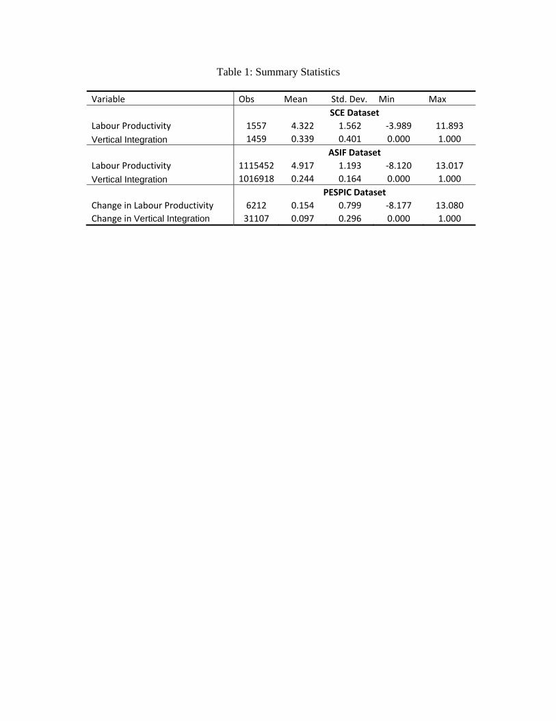
Table 1: Summary Statistics Variable  Obs Mean Std. Dev. Min  Max    SCE Dataset

Labour Productivity  1557 4.322 1.562 ‐3.989  11.893

Vertical Integration 1459 0.339 0.401 0.000  1.000

   ASIF Dataset

Labour Productivity  1115452 4.917 1.193 ‐8.120  13.017

Vertical Integration 1016918 0.244 0.164 0.000  1.000

   PESPIC Dataset

Change in Labour Productivity  6212 0.154 0.799 ‐8.177  13.080

Change in Vertical Integration  31107 0.097 0.296 0.000  1.000

Table 2: Analysis of the SCE Dataset, OLS Benchmark

1 2 3 4 Dependent Variable Labour Productivity Self-Made Input Percentage -0.307*** -0.278*** -0.298*** -0.237*** [0.100] [0.079] [0.079] [0.086] Firm Characteristics Firm Size 0.200*** 0.181*** 0.110*** [0.037] [0.038] [0.036] Firm Age -0.526*** -0.458*** -0.413*** [0.062] [0.069] [0.066] Percentage of Private Ownership 0.442*** 0.253* 0.268**

[0.130] [0.132] [0.122]

Capital Intensity 0.383*** 0.384*** 0.347***

[0.037] [0.034] [0.036]

CEO Characteristics Human Capital Education 0.041*** 0.040**

[0.016] [0.016]

Years of Being CEO 0.018** 0.007

[0.007] [0.007]

Deputy CEO Previously -0.004 -0.008

[0.070] [0.068]

Political Capital Government Cadre Previously 0.019 0.090

[0.222] [0.231]

Communist Party Member -0.192** -0.096

[0.082] [0.077]

Government Appointment -0.348*** -0.317***

[0.088] [0.092]

Industry Dummy Yes Yes Yes Yes City Dummy Yes No. of Observation 1,451 1,431 1,410 1,410

Robust standard errors, clustered at industry-city level, are reported in the bracket. *, **, and *** represent significance at 10%, 5%, and 1% level, respectively.

Table 3: Analysis of the SCE Dataset, IV Estimates

1 2

Panel A, Second Stage: Dependent Variable is Labour Productivity Self-Made Input Percentage -13.290** -5.182* [6.360] [2.803] Firm Characteristics Firm Size 0.180*** [0.063] Firm Age -0.291** [0.127] Percentage of Private Ownership 0.371 [0.234] Capital Intensity 0.323*** [0.054] CEO Characteristics Human Capital Education 0.061** [0.030] Years of Being CEO 0.033* [0.020] Deputy CEO Previously 0.096 [0.146] Political Capital Government Cadre Previously -0.451 [0.448] Communist Party Membership -0.24 [0.180] Government Appointment -0.408** [0.173] Industry Dummy Yes Yes City Dummy Yes

Panel B, First Stage: Dependent Variable is Self-Made Input Percentage Local Purchase 0.066** 0.067** [0.030] [0.029] Firm Characteristics Firm Size 0.016* [0.009] Firm Age 0.021 [0.018] Percentage of Private Ownership 0.019 [0.033] Capital Intensity -0.003 [0.008] CEO Characteristics Human Capital Education 0.005 [0.005] Years of Being CEO 0.005** [0.003]

Deputy CEO Previously 0.025 [0.025] Political Capital Government Cadre Previously -0.105* [0.059] Communist Party Membership -0.029 [0.030] Government Appointment -0.022 [0.025] Industry Dummy Yes Yes City Dummy Yes

Panel C, Various First-Stage Statistical Tests Relevance Test Anderson Canonical Correlation LR Statistic [4.96]** [4.57]** Cragg-Donald Wald Statistic [4.83]** [4.48]** Weak Instrument Test F Test of Excluded Instrument [4.95]** [5.25]** Anderson-Rubin Wald Test [43.67]*** [9.13]***

Stock-Wright LM S Statistic [23.07]*** [8.05]***

Number of Observations 1,445 1,404 Note: Robust standard errors, clustered at industry-city level, are presented in the bracket. *, **, *** represent significance at 10%, 5%, 1% level respectively.

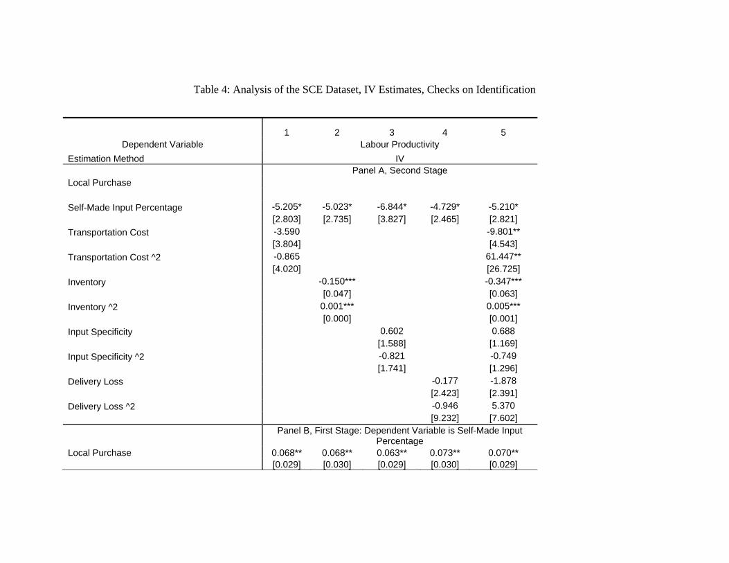
Table 4: Analysis of the SCE Dataset, IV Estimates, Checks on Identification

1 2 3 4 5 Dependent Variable Labour Productivity

Estimation Method IV Panel A, Second Stage Local Purchase

Self-Made Input Percentage -5.205* -5.023* -6.844* -4.729* -5.210*

[2.803] [2.735] [3.827] [2.465] [2.821]

Transportation Cost -3.590 -9.801**

[3.804] [4.543]

Transportation Cost ^2 -0.865 61.447**

[4.020] [26.725]

Inventory -0.150*** -0.347***

[0.047] [0.063]

Inventory ^2 0.001*** 0.005***

[0.000] [0.001]

Input Specificity 0.602 0.688

[1.588] [1.169]

Input Specificity ^2 -0.821 -0.749

[1.741] [1.296]

Delivery Loss -0.177 -1.878

[2.423] [2.391]

Delivery Loss ^2 -0.946 5.370

[9.232] [7.602]

Panel B, First Stage: Dependent Variable is Self-Made Input

Percentage Local Purchase 0.068** 0.068** 0.063** 0.073** 0.070** [0.029] [0.030] [0.029] [0.030] [0.029]

Note: Robust standard errors, clustered at industry-city level, are presented in the bracket. *, **, *** represent significance at 10%, 5%, 1% level respectively. The first Stage of the two-step GMM estimation contains same controls as the second stage but results of these control variables are not reported to save space (available upon request).

Panel C, Various First Stage Statistical Tests

Relevance Test Anderson Canonical Correlation LR Statistic [4.66]** [4.65]** [3.83]** [5.35]** [4.73]** Cragg-Donald Wald Statistic [4.58]** [4.55]** [3.80]** [5.25]** [4.72]** Weak Instrument Test F Test of Excluded Instrument [5.34]** [5.27]** [4.69]** [6.19]** [5.81]** Anderson-Rubin Wald test [9.88]*** [9.05]*** [12.99]*** [8.81]*** [11.54]*** Stock-Wright LM S statistic [8.70]*** [8.22]*** [10.69]*** [7.80]** [10.04]***

Included Control Variables Firm Characteristics Yes Yes Yes Yes Yes CEO Characteristics Yes Yes Yes Yes Yes Industry Dummy Yes Yes Yes Yes Yes City Dummy Yes Yes Yes Yes Yes

Number of Observations 1,401 1,403 1,307 1,391 1,281

Table 5: Analysis of the SCE Dataset, Robustness Checks

1 2 3 4 5 6 Dependent Variable Labour Productivity Sample Exclusion of Outliers Focused Businesses Private Firms Estimation Method OLS IV OLS IV OLS IV Self-Made Input Percentage -0.200** -5.897* -0.302*** -4.051* -0.210** -7.246 [0.085] [3.174] [0.087] [2.225] [0.099] [7.301]

Included Control Variables Firm Characteristics Yes Yes Yes Yes Yes Yes CEO Characteristics Yes Yes Yes Yes Yes Yes Industry Dummy Yes Yes Yes Yes Yes Yes City Dummy Yes Yes Yes Yes Yes Yes

Number of Observations 1,380 1,374 1,298 1,292 1,151 1,148 Note: Robust standard errors, clustered at industry-city level, are presented in the bracket. *, **, *** represent significance at 10%, 5%, 1% level respectively.

Table 6: Analysis of the ASIF Dataset, Main Results

1 2 3 4

Dependent Variable Labour Productivity

Estimation Pooled OLS Panel Fixed-Effect Panel Fixed-Effect Anderson-Hsiao IV

Value Added Ratio -1.274*** -0.627*** -0.552*** -0.470***

[0.011] [0.008] [0.009] [0.015]

Lagged Labour Productivity 0.176*** 0.286***

[0.003] [0.007] Year Dummy Yes Yes Yes Yes Industry Dummy Yes

Province Dummy Yes

Firm Dummy Yes Yes Yes

Number of Observations 943,257 943,257 634,141 398,380 Note: Robust standard errors, clustered at firm level, are presented in the bracket. *, **, *** represent significance at 10%, 5%, 1% level respectively.

Table 7: Analysis of the ASIF Dataset, Robustness Checks

1 2 3 4 5 6 7 8

Dependent Variable Labour Productivity

Sample Balanced Exclusion of Outliers Private Firms Whole

Estimation Panel Fixed-

Effect Anderson-Hsiao IV

Panel Fixed-Effect

Anderson-Hsiao IV

Panel Fixed-Effect

Anderson-Hsiao IV

Panel Fixed-Effect

Anderson-Hsiao IV

Value Added Ratio -0.460*** -0.467*** -0.397*** -0.679*** -0.479*** -0.485*** -0.558*** -0.502***

[0.014] [0.023] [0.007] [0.016] [0.011] [0.017] [0.009] [0.016]

Lagged Labour Productivity 0.347*** 0.374*** 0.164*** 0.529*** 0.126*** 0.334*** 0.175*** 0.381***

[0.005] [0.013] [0.002] [0.007] [0.003] [0.008] [0.003] [0.007]

Capital Intensity 0.193*** 0.026***

[0.002] [0.001] Year Dummy Yes Yes Yes Yes Yes Yes Yes Yes Firm Dummy Yes Yes Yes Yes Yes Yes Yes Yes

Number of Observations 187,992 148,344 575,174 362,682 395,902 253,080 630,027 396,066 Note: Robust standard errors, clustered at firm level, are presented in the bracket. *, **, *** represent significance at 10%, 5%, 1% level respectively.

Table 8: Analysis of the PESPIC Dataset, Main Results

1 2 3 4 5 6

Dependent Variable Change in Labour Productivity

Change in Vertical Integration -0.091** -0.095** -0.095** -0.095** -0.092** -0.076**

[0.036] [0.037] [0.037] [0.037] [0.036] [0.037]

Initial Firm Size 0.085*** 0.084*** 0.084*** 0.085*** 0.085*** 0.076***

[0.026] [0.026] [0.026] [0.026] [0.026] [0.025]

Initial Sales Change 0.027*** 0.026*** 0.027*** 0.027*** 0.027*** 0.017**

[0.008] [0.008] [0.009] [0.009] [0.009] [0.008]

Introduction of New Technology 0.018 0.019 0.018 0.022 0.005

[0.028] [0.028] [0.028] [0.029] [0.029]

Introduction of New Joint Venture -0.024 -0.029 -0.027 0.014

[0.058] [0.064] [0.064] [0.056]

Introduction of New Licensing Agreement 0.016 0.018 -0.003

[0.054] [0.054] [0.052]

Introduction of New Major Product Line -0.018 -0.002

[0.027] [0.026]

Change in Capital Intensity 0.258***

[0.045]

Number of Observations 2,672 2,671 2,670 2,670 2,670 2,583 Note: Robust standard errors, clustered at firm level, are presented in the bracket. *, **, *** represent significance at 10%, 5%, 1% level respectively.

Table 9: Analysis of the PESPIC Dataset, Robustness Checks

1 2

Dependent Variable Change in Labour Productivity

Sample Exclusion of Outlying Observations Private Firms

Change in Vertical Integration -0.057*** -0.090**

[0.021] [0.036]

Initial Firm Size 0.084*** 0.085***

[0.022] [0.026]

Initial Sales Change 0.035*** 0.026***

[0.006] [0.008]

Number of Observations 2,637 2,658 Note: Robust standard errors, clustered at firm level, are presented in the bracket. *, **, *** represent significance at 10%, 5%, 1% level respectively.