Winter Quarter 2008Christopher T. Russell

Raymond J. Walker

Date

Topic1/7 Organization and Introduction

to Space Physics I1/9 Introduction to Space Physics II1/14 Introduction to Space Physics III1/16 The Sun I1/23 The Sun II1/25

The Solar Wind I1/28 The Solar Wind II2/ 1 First Exam2/4 Bow Shock and Magnetosheath2/6 The Magnetosphere I

ESS 200C -

Space Plasma Physics

Date

Topic2/11 The Magnetosphere II2/16 The Magnetosphere III2/20 Planetary Magnetospheres2/22 The Earth’s Ionosphere2/25 Substorms2/27 Aurorae3/3 Planetary Ionospheres3/5 Pulsations and waves3./10 Storms and Review3/12 Second Exam

Schedule of Classes

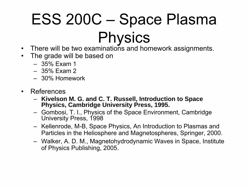
ESS 200C –

Space Plasma Physics

•

There will be two examinations and homework assignments.•

The grade will be based on–

35% Exam 1–

35% Exam 2–

30% Homework

•

References–

Kivelson M. G. and C. T. Russell, Introduction to Space Physics, Cambridge University Press, 1995.

–

Gombosi, T. I., Physics of the Space Environment, Cambridge University Press, 1998

–

Kellenrode, M-B, Space Physics, An Introduction to Plasmas and Particles in the Heliosphere

and Magnetospheres, Springer, 2000.–

Walker, A. D. M., Magnetohydrodynamic Waves in Space, Institute of Physics Publishing, 2005.

Space Plasma Physics

•

Space physics is concerned with the interaction of charged particles with electric and magnetic fields in space.

•

Space physics involves the interaction between the Sun, the solar wind, the magnetosphere and the ionosphere.

•

Space physics started with observations of the aurorae.–

Old Testament references to auroras.

–

Greek literature speaks of “moving accumulations of burning clouds”

–

Chinese literature has references to auroras prior to 2000BC

•

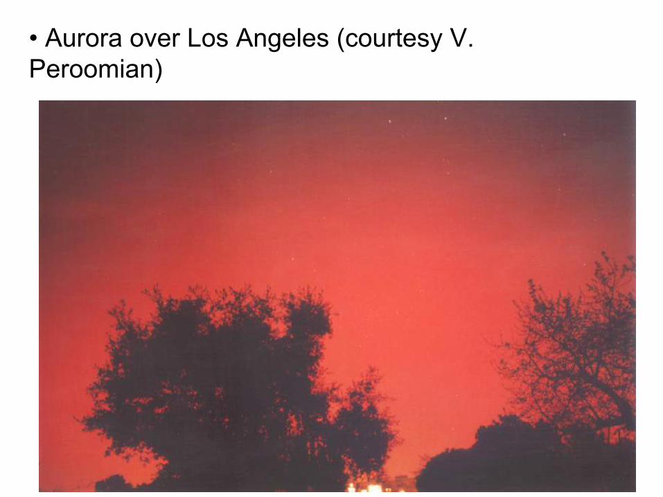
Aurora over Los Angeles (courtesy V. Peroomian)

–

Galileo theorized that aurora is caused by air rising out of the Earth’s shadow to where it could be illuminated by sunlight. (Note he also coined the name aurora borealis meaning “northern dawn”.)

–

Descartes thought they are reflections from ice crystals.–

Halley suggested that auroral phenomena are ordered by the Earth’s magnetic field.

–

In 1731 the French philosopher de Mairan

suggested they are connected to the solar atmosphere.

•

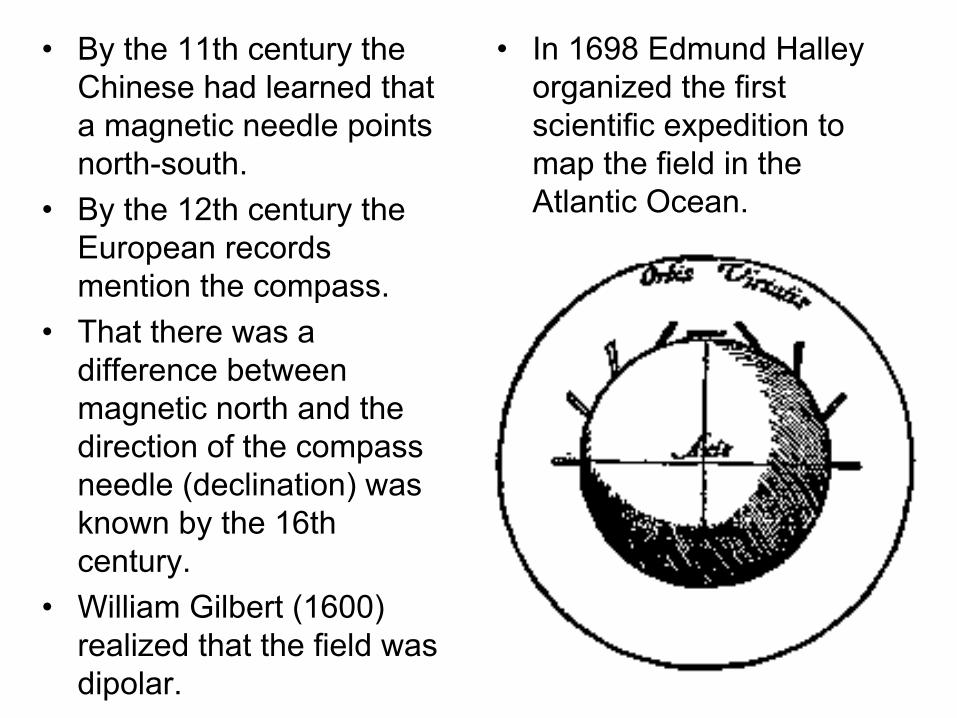
By the 11th century the Chinese had learned that a magnetic needle points north-south.

•

By the 12th century the European records mention the compass.

•

That there was a difference between magnetic north and the direction of the compass needle (declination) was known by the 16th century.

•

William Gilbert (1600) realized that the field was dipolar.

•

In 1698 Edmund Halley organized the first scientific expedition to map the field in the Atlantic Ocean.

The Plasma State

•

A plasma is an electrically neutral ionized gas.–

The Sun is a plasma

–

The space between the Sun and the Earth is “filled” with a plasma.

–

The Earth is surrounded by a plasma.–

A stroke of lightning forms a plasma

–

Over 99% of the Universe is a plasma.•

Although neutral a plasma is composed of charged particles-

electric and magnetic

forces are critical for understanding plasmas.

The Motion of Charged Particles

•

Equation of motion

•

SI Units–

mass (m) -

kg–

length (l) -

m–

time (t) -

s–

electric field (E) -

V/m–

magnetic field (B) -

T–

velocity (v) -

m/s–

Fg

stands for non-electromagnetic forces (e.g. gravity) -

usually ignorable.

gFBvqEqdtvdm

rrrrr

+×+=

•

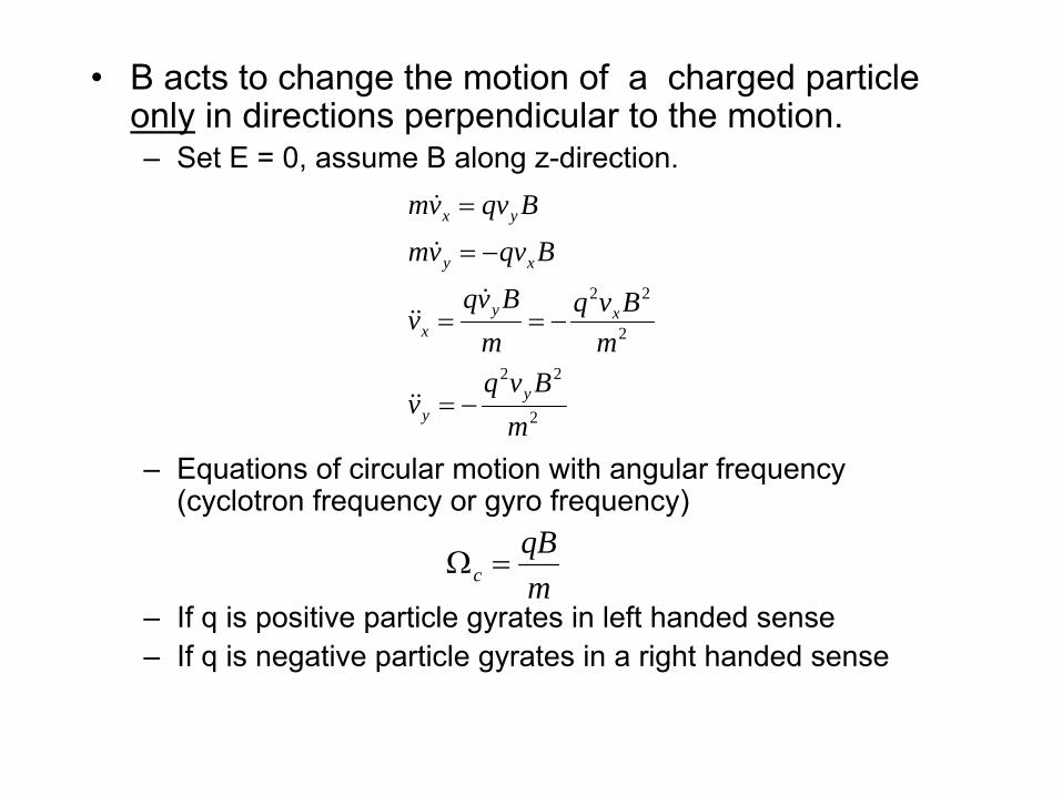
B acts to change the motion of a charged particle only

in directions perpendicular to the motion.

–

Set E = 0, assume B along z-direction.

–

Equations of circular motion with angular frequency (cyclotron frequency or gyro frequency)

–

If q is positive particle gyrates in left handed sense–

If q is negative particle gyrates in a right handed sense

2

22

2

22

mBvq

v

mBvq

mBvq

v

Bqvvm

Bqvvm

yy

xyx

xy

yx

−=

−==

−=

=

&&

&&&

&

&

mqB

c =Ω

•

Radius of circle ( rc

) -

cyclotron radius or Larmor radius or gyro radius.

–

The gyro radius is a function of energy.–

Energy of charged particles is usually given in electron volts (eV)

–

Energy that a particle with the charge of an electron gets in falling through a potential drop of 1 Volt-

1 eV

= 1.6X10-19

Joules (J).•

Energies in space plasmas go from electron Volts to kiloelectron

Volts (1 keV

= 103 eV) to millions of electron Volts (1 meV

= 106

eV)•

Cosmic ray energies go to gigaelectron

Volts ( 1 geV

= 109 eV).

•

The circular motion does no work on a particle

qBmv

v

c

cc

⊥

⊥

=

Ω=

ρ

ρ

0)()( 221

=×⋅==⋅=⋅ Bvvqdtmvdv

dtvdmvF

rrrrr

rr

Only the electric field can energize particles!

•

The electric field can modify the particles motion.–

Assume but still uniform and Fg

=0.–

Frequently in space physics it is ok to set•

Only can accelerate particles along•

Positive particles go along and negative particles go along

•

Eventually charge separation wipes out–

has a major effect on motion. •

As a particle gyrates it moves along and gains energy •

Later in the circle it losses energy.•

This causes different parts of the “circle” to have different radii -

it doesn’t close on itself.

•

Drift velocity is perpendicular to and•

No charge dependence, therefore no currents

0≠Er

0=⋅ BErr

Er

Br

EE−

E

⊥EEr

2BBEuE

rrr ×

=

Er

Br

Br

•

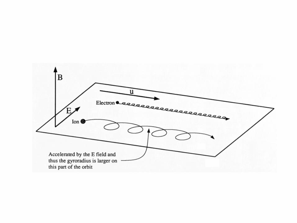
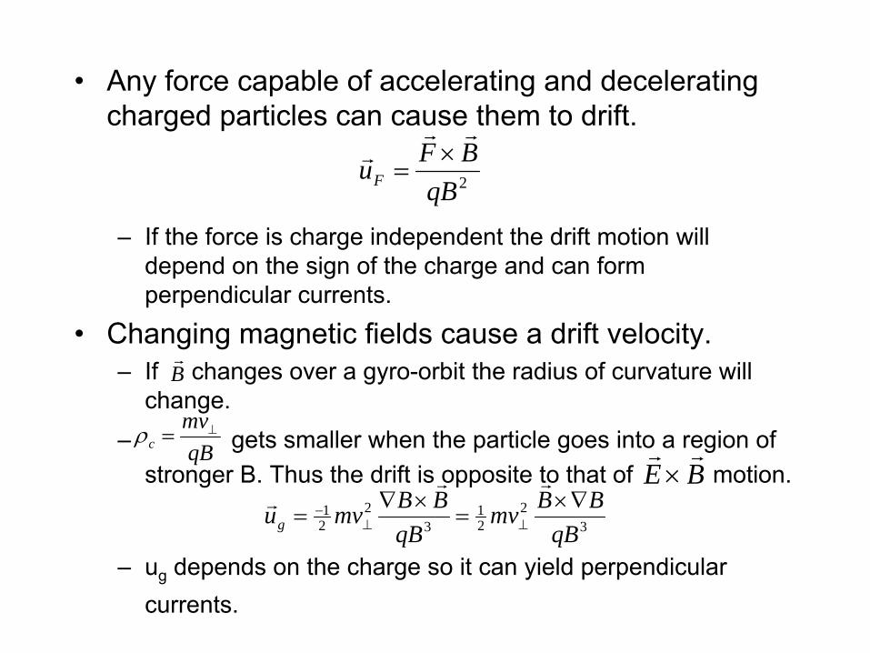
Any force capable of accelerating and decelerating charged particles can cause them to drift.

–

If the force is charge independent the drift motion will depend on the sign of the charge and can form perpendicular currents.

•

Changing magnetic fields cause a drift velocity.–

If changes over a gyro-orbit the radius of curvature will change.

–

gets smaller when the particle goes into a region of stronger B. Thus the drift is opposite to that of motion.

–

ug

depends on the charge so it can yield perpendicular currents.

2qBBFuF

rrr ×

=

Br

qBmv

c⊥=ρ

BErr

×

32

21

32

21

qBBBmv

qBBBmvug

∇×=

×∇= ⊥⊥

−

rrr

•

The change in the direction of the magnetic field along a field line can cause motion.–

The curvature of the magnetic field line introduces a drift motion.

•

As particles move along the field they undergo centrifugal acceleration.

•

Rc

is the radius of curvature of a field line ( ) where

, is perpendicular to and points away from the center of curvature, is the component of velocity along

•

Curvature drift can cause currents.

cc

RR

mvF ˆ

2

=r

bbRn

c

ˆ)ˆ(ˆ

∇⋅−=

BBbr

=ˆ n̂ Br

v Br

2

2

2

2 ˆˆ)ˆ(

qBR

nBmv

qB

bbBmvu

cc

×−=

∇⋅×=

rrr

•

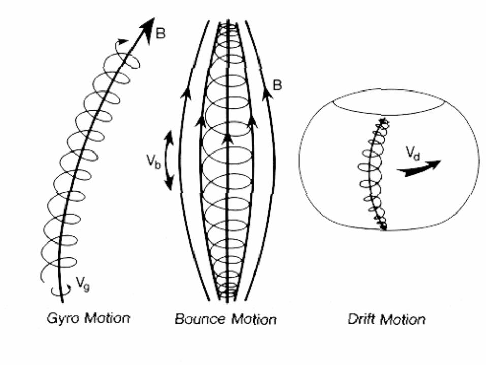
The Concept of the Guiding Center–

Separates the motion ( ) of a particle into motion perpendicular ( ) and parallel ( ) to the magnetic field.

–

To a good approximation the perpendicular motion can consist of a drift ( ) and the gyro-motion ( )

–

Over long times the gyro-motion is averaged out and the particle motion can be described by the guiding center motion consisting of the parallel motion and drift. This is very

useful for distances l such that and time scales τ such that

vr

⊥v v

Dvc

vΩ

ccvvvvvvvv gcD ΩΩ⊥ +=++=+=rrrrrrrr

1<<lcρ( ) 11 <<Ω −τ

•

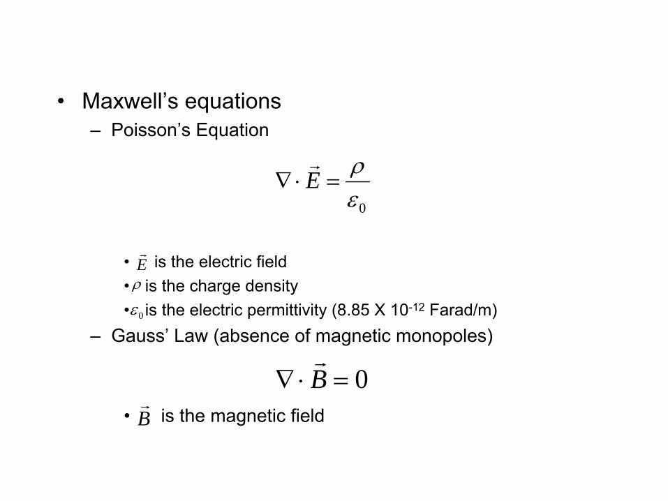
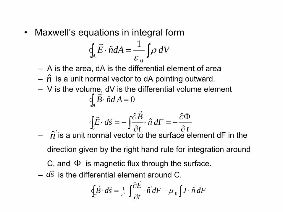
Maxwell’s equations–

Poisson’s Equation

•

is the electric field•

is the charge density•

is the electric permittivity (8.85 X 10-12

Farad/m)–

Gauss’ Law (absence of magnetic monopoles)

•

is the magnetic field

0ερ

=⋅∇ Er

Er

0=⋅∇ Br

Br

ρ

0ε

–

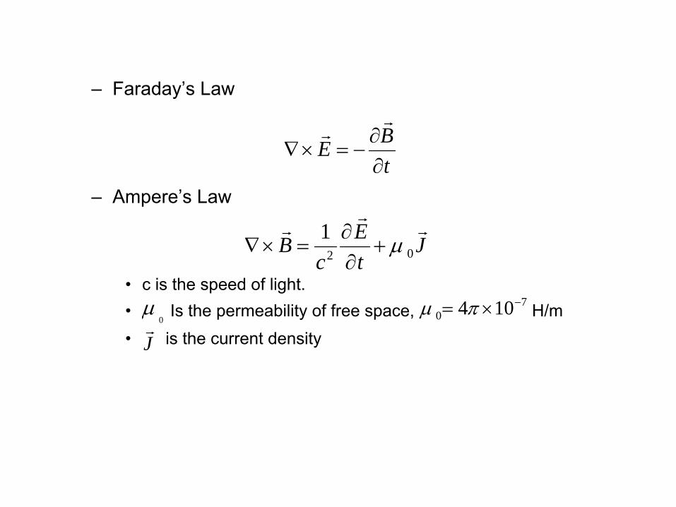
Faraday’s Law

–

Ampere’s Law

•

c is the speed of light.•

Is the permeability of free space, H/m•

is the current density

tBE

∂∂

−=×∇r

r

JtE

cB

rr

r02

1 μ+∂∂

=×∇

0μ 7

0 104 −×= πμ

Jr

•

Maxwell’s equations in integral form

–

A is the area, dA

is the differential element of area–

is a unit normal vector to dA

pointing outward.–

V is the volume, dV

is the differential volume element

–

is a unit normal vector to the surface element dF

in the

direction given by the right hand rule for integration around

C, and is magnetic flux through the surface. –

is the differential element around C.

∫∫ =⋅ dVdAnEA

ρε 0

1ˆr

n̂

tdFn

tBsdE

AdnB

C

A

∂Φ∂

−=⋅∂∂

−=⋅

=⋅

∫∫

∫'ˆ

0ˆr

rv

r

'n̂

sdr

dFnJdFntEsdB

cC ∫∫∫ ⋅+⋅∂∂

=⋅ '0

'1 ˆˆ2 μr

rr

Φ

•

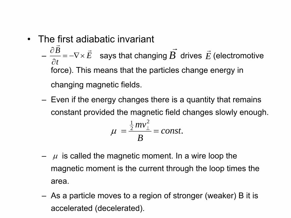
The first adiabatic invariant–

says that changing drives (electromotive

force). This means that the particles change energy in

changing magnetic fields.

–

Even if the energy changes there is a quantity that remains constant provided the magnetic field changes slowly enough.

–

is called the magnetic moment. In a wire loop the magnetic moment is the current through the loop times the area.

–

As a particle moves to a region of stronger (weaker) B it is accelerated (decelerated).

EtB rr

×−∇=∂∂

Er

.2

21

constBmv

== ⊥μ

μ

Br

•

For a coordinate in which the motion is periodic the action integral

is conserved. Here pi is the canonical momentum ( where A is the vector potential).

•

First term –•

Second term -

•

For a gyrating particle

•

The action integrals are conserved when the properties of the system change slowly compared to the period of the coordinate.

constant == ∫ iii dqpJ

μπqmsdpJ 2

1 =⋅= ∫ ⊥rr

Aqvmprrr

+=

qmmvdsmv μππρ 42 == ⊥⊥∫qm

qBvmSdBqSdAqsdAq μππ 22 22

−=−=⋅=⋅×∇=⋅ ∫∫ ∫∫∫ ⊥rrrrrr

•

The magnetic mirror–

As a particle gyrates the current will be

where

–

The force on a dipole magnetic moment is

where

cTqI =

ccT

Ω=

π2

μ

ππ

π

π ===

Ω==

⊥Ω

Ω

⊥

⊥

BmvIA

vrA

c

cqv

cc

2

2

2

2

22

2

2

dzdBBF μμ −=∇⋅−=

rr

b̂μμ =r

•

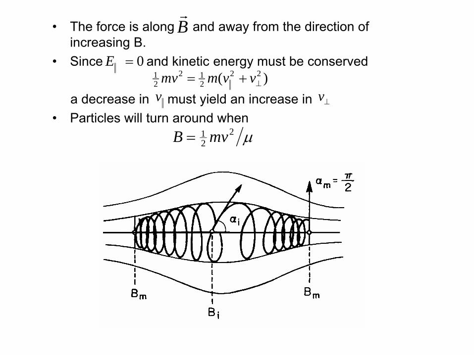
The force is along and away from the direction of increasing B.

•

Since and kinetic energy must be conserved

a decrease in must yield an increase in •

Particles will turn around when

Br

0=E

v ⊥v

μ221 mvB =

)( 22212

21

⊥+= vvmmv

•

The second adiabatic invariant–

The integral of the parallel momentum over one complete bounce between mirrors is constant (as long as B doesn’t change much in a bounce).

–

Using conservation of energy and the first adiabatic invariant

here Bm

is the magnetic field at the mirror point.

.22

1

constdsmvJs

s== ∫

.)1(2 212

1

constdsBBmvJ

s

sm

=−= ∫

–

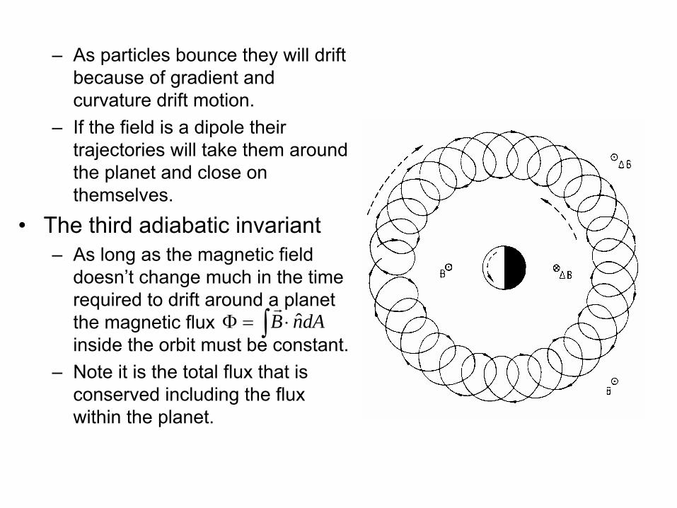
As particles bounce they will drift because of gradient and curvature drift motion.

–

If the field is a dipole their trajectories will take them around the planet and close on themselves.

•

The third adiabatic invariant–

As long as the magnetic field doesn’t change much in the time required to drift around a planet the magnetic flux inside the orbit must be constant.

–

Note it is the total flux that is conserved including the flux within the planet.

∫ ⋅=Φ dAnB ˆr

•

Limitations on the invariants–

is constant when there is little change in the field’s strength over a cyclotron path.

–

All invariants require that the magnetic field not change much in the time required for one cycle of motion

where is the orbit period.

τ11

<<∂∂

tB

B

ms

s

J

~1~

1010~ 36

Φ

−− −

ττ

τ μ

τ

μ

cBB

ρ1

<<∇

•

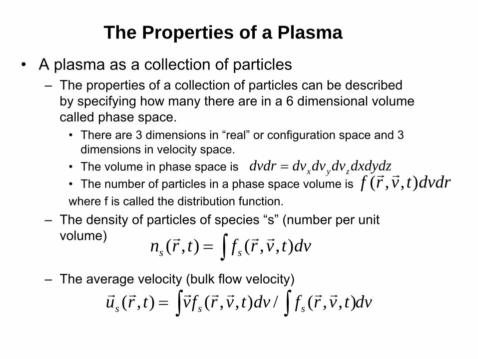
A plasma as a collection of particles–

The properties of a collection of particles can be described by specifying how many there are in a 6 dimensional volume called phase space.

•

There are 3 dimensions in “real” or configuration space and 3 dimensions in velocity space.

•

The volume in phase space is•

The number of particles in a phase space volume iswhere f is called the distribution function.

–

The density of particles of species “s” (number per unit volume)

–

The average velocity (bulk flow velocity)

dxdydzdvdvdvdvdr zyx=dvdrtvrf ),,( rr

dvtvrftrn ss ),,(),( rrr∫=

dvtvrfdvtvrfvtru sss ∫∫= ),,(/),,(),( rrrrrrr

The Properties of a Plasma

–

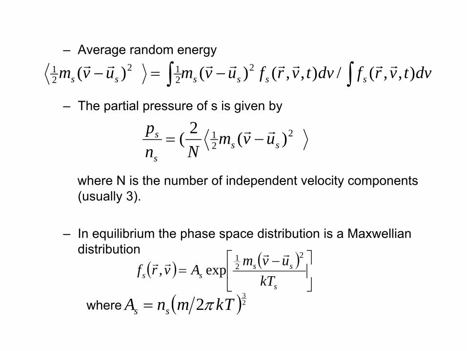
Average random energy

–

The partial pressure of s is given by

where N is the number of independent velocity components (usually 3).

–

In equilibrium the phase space distribution is a Maxwellian

distribution

where

( ) ( )⎥⎦

⎤⎢⎣

⎡ −=

s

ssss kT

uvmAvrf2

21

exp,rr

rr

∫∫ −=− dvtvrfdvtvrfuvmuvm ssssss ),,(/),,()()( 2212

21 rrrrrrrr

221 )(2( ss

s

s uvmNn

p rr−=

( )23

2 TkmnA ss π=

•

For monatomic particles in equilibrium

where k is the Boltzman

constant (k=1.38x10-23 JK-1)•

For monatomic particles in equilibrium

•

This is true even for magnetized particles.•

The ideal gas law becomes

( )( ) 2221

sss NkTuvm =−rr

2/)( 221 NkTuvm ss =−

rr

sss kTnp =

sss kTnp =

–

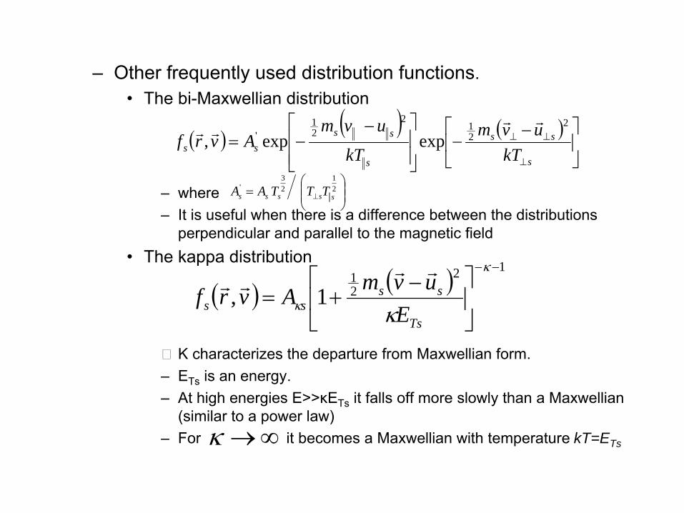
Other frequently used distribution functions.•

The bi-Maxwellian

distribution

–

where –

It is useful when there is a difference between the distributions perpendicular and parallel to the magnetic field

•

The kappa distribution

Κ characterizes the departure from Maxwellian form.–

ETs

is an energy.–

At high energies E>>κETs

it falls off more slowly than a Maxwellian

(similar to a power law)

–

For it becomes a Maxwellian

with temperature kT=ETs

( )( ) ( )

⎥⎦

⎤⎢⎣

⎡ −−

⎥⎥⎦

⎤

⎢⎢⎣

⎡ −−=

⊥

⊥⊥

s

ss

s

ssss kT

uvmkT

uvmAvrf

221

221

' expexp,rr

rr

( ) ( ) 1221

1,−−

⎥⎦

⎤⎢⎣

⎡ −+=

κ

κ κ Ts

ssss E

uvmAvrfrr

rr

∞→κ

⎟⎟⎠

⎞⎜⎜⎝

⎛= ⊥

21

23

'sssss TTTAA

•

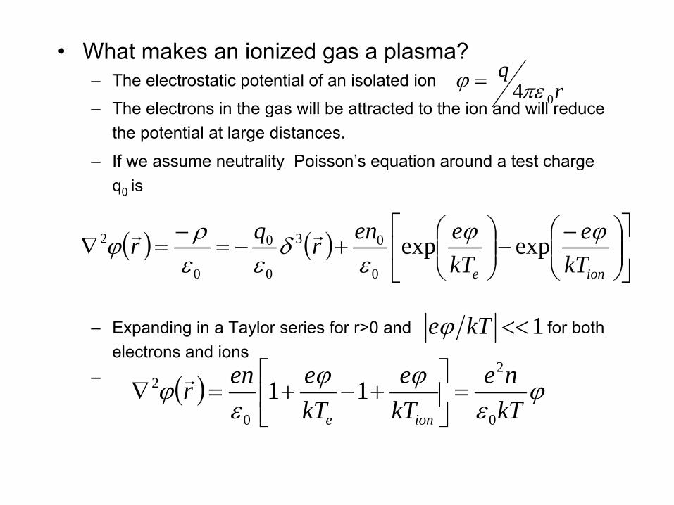
What makes an ionized gas a plasma?–

The electrostatic potential of an isolated ion–

The electrons in the gas will be attracted to the ion and will reduce the potential at large distances.

–

If we assume neutrality Poisson’s equation around a test charge

q0 is

–

Expanding in a Taylor series for r>0 and for both electrons and ions

–

( ) ( ) ⎥⎦

⎤⎢⎣

⎡⎟⎟⎠

⎞⎜⎜⎝

⎛ −−⎟⎟

⎠

⎞⎜⎜⎝

⎛+−=

−=∇

ione kTe

kTeenrqr ϕϕ

εδ

εερϕ expexp

0

03

0

0

0

2 rr

rq

04πεϕ =

1<<kTeϕ

( ) ϕε

ϕϕε

ϕkTne

kTe

kTeenr

ione 0

2

0

2 11 =⎥⎦

⎤⎢⎣

⎡+−+=∇

r

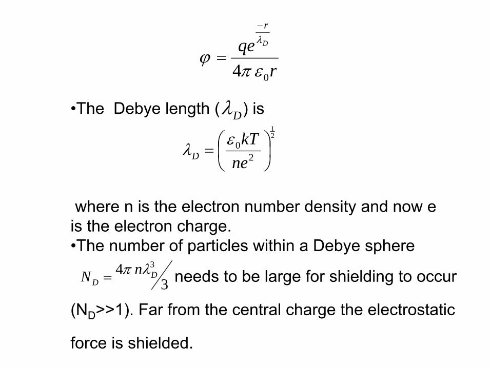
•The Debye

length ( ) is

where n is the electron number density and now e is the electron charge.•The number of particles within a Debye

sphere

needs to be large for shielding to occur

(ND

>>1). Far from the central charge the electrostatic

force is shielded.

rqe D

r

04 επϕ

λ−

=

34 3

DD

nN λπ=

Dλ21

20 ⎟

⎠⎞

⎜⎝⎛=

nekT

Dελ

•

The plasma frequency–

Consider a slab of plasma of thickness L.–

At t=0 displace the electron part of the slab by <<L and the ion part of the slab by <<L in the opposite direction.

–

Poisson’s equation gives

–

The equations of motion for the electron and ion slabs are

ie δδδ −=

δε0

0enE =

δεε

δδδ

δ

δ

)(0

02

0

02

2

2

2

2

2

2

2

2

2

2

ione

ie

iion

ee

mne

mne

dtd

dtd

dtd

eEdtdm

eEdt

dm

+−=−=

=

−=

eδiδ

–

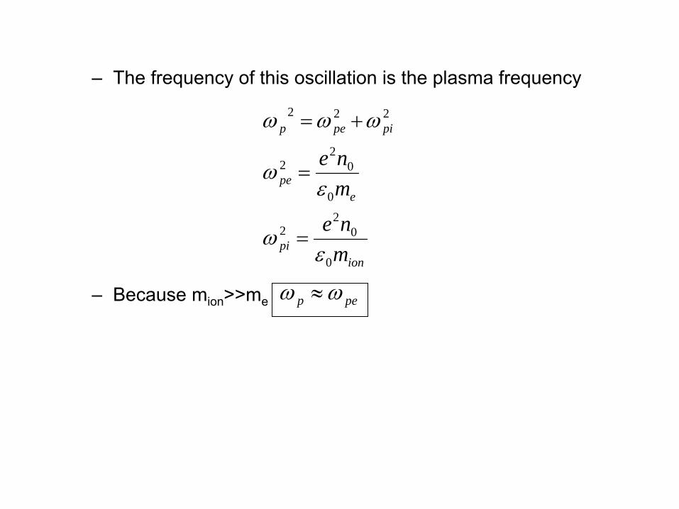
The frequency of this oscillation is the plasma frequency

–

Because mion

>>me

ionpi

epe

pipep

mne

mne

0

02

2

0

02

2

222

εω

εω

ωωω

=

=

+=

pep ωω ≈

•

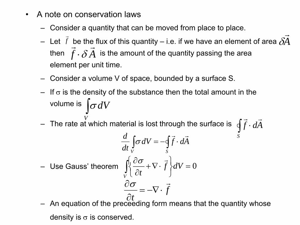
A note on conservation laws–

Consider a quantity that can be moved from place to place.

–

Let be the flux of this quantity –

i.e. if we have an element of area then is the amount of the quantity passing the area element per unit time.

–

Consider a volume V of space, bounded by a surface S.

–

If σ is the density of the substance then the total amount in the volume is

–

The rate at which material is lost through the surface is

–

Use Gauss’ theorem

–

An equation of the preceeding

form means that the quantity whose

density is σ

is conserved.

fr

Ar

δAfrr

δ⋅

∫V

dVσ

∫ ⋅S

Adfrr

∫ ∫ ⋅−=V S

AdfdVdtd rr

σ

0=⎭⎬⎫

⎩⎨⎧ ⋅∇+

∂∂

∫ dVftV

rσ

ft

r⋅−∇=

∂∂σ

•

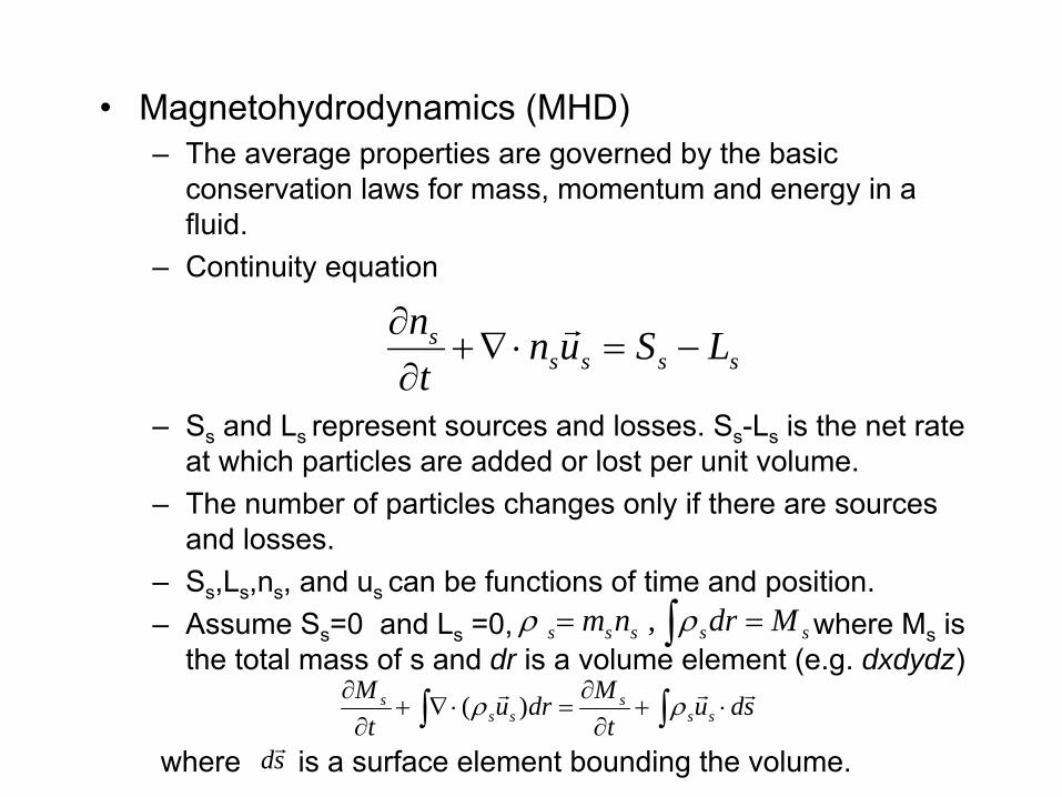
Magnetohydrodynamics (MHD)–

The average properties are governed by the basic conservation laws for mass, momentum and energy in a fluid.

–

Continuity equation

–

Ss

and Ls represent sources and losses. Ss

-Ls

is the net rate at which particles are added or lost per unit volume.

–

The number of particles changes only if there are sources and losses.

–

Ss

,Ls

,ns

, and us can be functions of time and position.–

Assume Ss

=0 and Ls

=0, where Ms

is the total mass of s and dr is a volume element (e.g. dxdydz)

where is a surface element bounding the volume.

sssss LSuntn

−=⋅∇+∂

∂ r

sssss Mdrnm == ∫ ρρ ,

sdut

Mdrut

Mss

sss

s rrr⋅+

∂∂

=⋅∇+∂

∂∫∫ ρρ )(

sdr

–

Momentum equation

where is the charge density, is the current density, and the last term is the density of non-

electromagnetic forces.–

The operator is called the convective derivative and gives the total time derivative resulting from intrinsic time changes and spatial motion.

–

If the fluid is not moving (us =0) the left side gives the net change in the momentum density of the fluid element.

–

The right side is the density of forces•

If there is a pressure gradient then the fluid moves toward lower pressure.

•

The second and third terms are the electric and magnetic forces.

sgssqsssssssss

s mFBJEpLSumuut

u ρρρ +×++−∇=−+∇⋅+∂

∂ rrrrrrr

)()(

ssqs nq=ρ ssss unqJ rr=

)( ∇⋅+∂∂

sut

r

( )( ) sgssqssssstu mFBJEpuuss

rrrrrrr

ρρρρ +×++−∇=⋅∇+∂∂

–

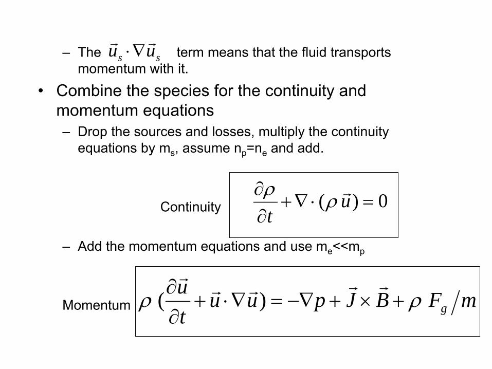
The term means that the fluid transports momentum with it.

•

Combine the species for the continuity and momentum equations–

Drop the sources and losses, multiply the continuity equations by ms

, assume np

=ne

and add.

Continuity

–

Add the momentum equations and use me

<<mp

Momentum

ss uu rr∇⋅

0)( =⋅∇+∂∂ u

trρρ

mFBJpuutu

gρρ +×+−∇=∇⋅+∂∂ rrrrr

)(

•

Energy equation

where is the heat flux, U is the internal energy density of the monatomic plasma and N is the number of degrees of freedom–

adds three unknowns to our set of equations. It is usually treated by making approximations so it can be handled by the other variables.

–

Many treatments make the adiabatic assumption (no change in the entropy of the fluid element) instead of using the energy equation

or

where cs

is the speed of sound and cp

and cv

are the specific heats at constant pressure and constant volume. It is called the polytropic

index. In thermodynamic equilibrium

mFuEJqupuUuUut g

rrrrrrr⋅+⋅=+++⋅∇++

∂∂ ρρρ ])[()( 2

212

21

)2/( nNkTU =qr

qr

.constp =−γρ)(2 ρρ

∇⋅+∂∂

=∇⋅+∂∂ u

tcpu

tp

srr

ργ pcs =2vp cc=γ

3/5)2( =+= NNγ

•

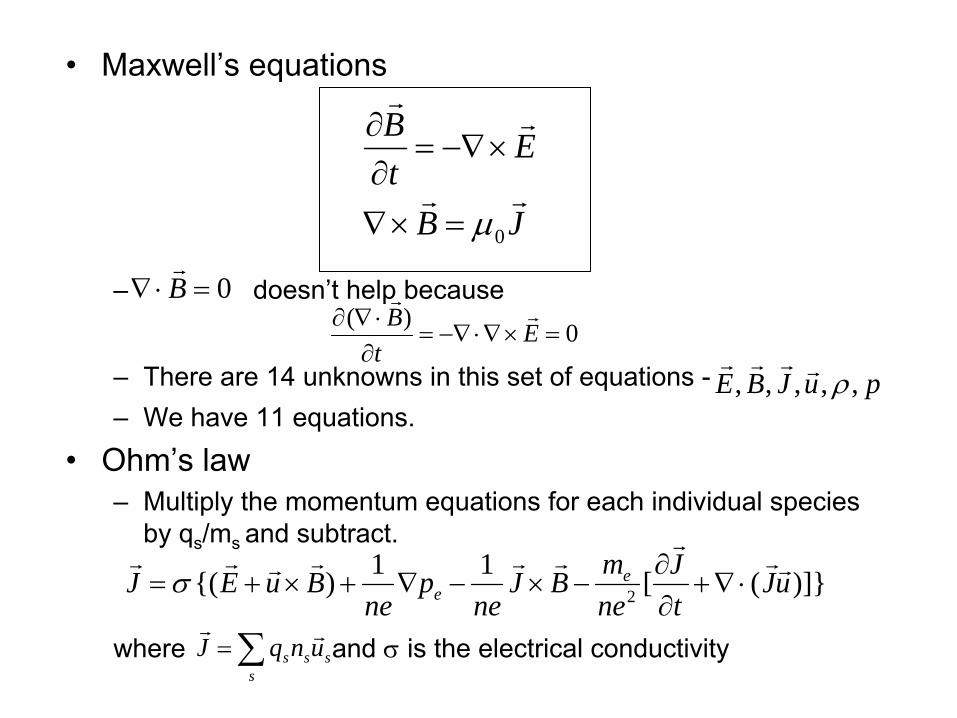
Maxwell’s equations

–

doesn’t help because

–

There are 14 unknowns in this set of equations -–

We have 11 equations.

•

Ohm’s law–

Multiply the momentum equations for each individual species by qs

/ms and subtract.

where and σ

is the electrical conductivity

JB

EtB

rr

rr

0μ=×∇

×−∇=∂∂

0=⋅∇ Br

0)(=×∇⋅−∇=

∂⋅∇∂ EtB rr

puJBE ,,,,, ρrrrr

)]}([11){( 2 uJtJ

nemBJ

nep

neBuEJ e

err

rrrrrrr

⋅∇+∂∂

−×−∇+×+= σ

sss

s unqJ rr∑=

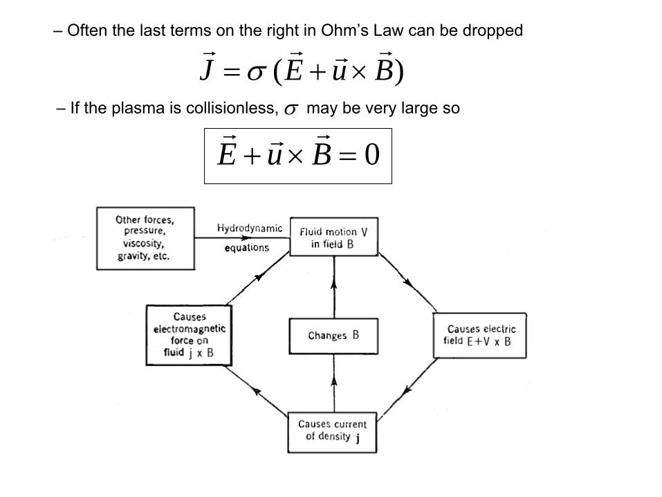
– Often the last terms on the right in Ohm’s Law can be dropped

– If the plasma is collisionless, may be very large soσ)( BuEJrrrr

×+= σ

0=×+ BuErrr

•

Frozen in flux–

Combining Faraday’s law ( ), and

Ampere’ law ( ) with

where is the magnetic viscosity–

If the fluid is at rest this becomes a “diffusion” equation

–

The magnetic field will exponentially decay (or diffuse) from a

conducting medium in a time where LB is the system size.

tBE

∂∂

−=×∇r

r

JBrr

0μ=×∇

BButB

m

rrrr

2)( ∇+××∇=∂∂ η

01 μση =m

BtB

m

rr

2∇=∂∂ η

mBD L ητ 2=

)( BuEJrrrr

×+= σ

–

On time scales much shorter than

–

The electric field vanishes in the frame moving with the fluid.–

Consider the rate of change of magnetic flux

–

The first term on the right is caused by the temporal changes in B

–

The second term is caused by motion of the boundary–

The term is the area swept out per unit time–

Use the identity and Stoke’s

theorem

–

If the fluid is initially on surface s as it moves through the system the flux through the surface will remain constant even though the location and shape of the surface change.

)( ButB rrr

××∇=∂∂

∫∫ ∫ ×⋅+⋅∂∂

=⋅=Φ

CA AlduBdAn

tBdAnB

dtd

dtd )(ˆˆ

rrrr

r

ldurr

×

0ˆ)( =⋅⎟⎟⎠

⎞⎜⎜⎝

⎛××∇−

∂∂

=Φ

∫ dAnButB

dtd

A

rrr

Dτ

BACCBArrrrrr

×⋅=×⋅

•

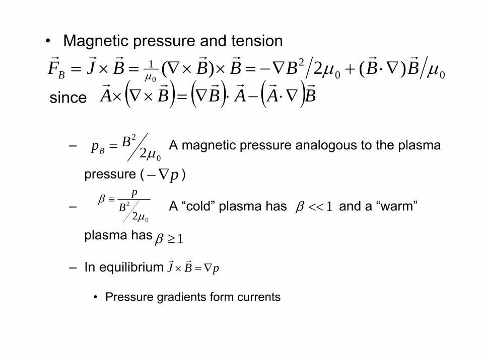
Magnetic pressure and tension

since

–

A magnetic pressure analogous to the plasma

pressure ( )

–

A “cold” plasma has and a “warm”

plasma has

–

In equilibrium

•

Pressure gradients form currents

0021 )(2)(

0μμμ BBBBBBJFB

rrrrrrr∇⋅+∇−=××∇=×=

0

2

2μBpB =

p∇−

0

2

2μβ

Bp

≡ 1<<β

1≥β

pBJ ∇=×rr

( ) ( ) ( )BAABBArrrrrr

∇⋅−⋅∇=×∇×

– cancels the parallel component

of the term. Thus only the perpendicular component of the magnetic pressure exerts a force on the plasma.

–

is the magnetic tension and is

directed antiparallel

to the radius of curvature (RC

) of the

field line. Note that is directed outward.

0

2

0 2ˆˆˆ

μμBbbBBb ∇=∇⋅

r

0

2

2μB∇−

)ˆ

(ˆˆ)(0

2

0

2

CRBnbbB

μμ −=∇⋅

n̂

– The second term in can be written as a sum of two terms

bbBBBbBB ˆˆ)(ˆ])[(0

2

00∇⋅+∇⋅=∇⋅

μμμrrrBJrr

×

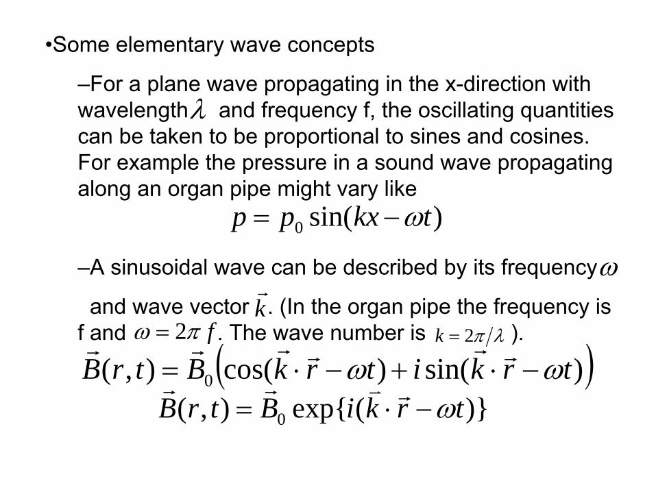
•Some elementary wave concepts

–For a plane wave propagating in the x-direction with wavelength and frequency f, the oscillating quantities can be taken to be proportional to sines

and cosines.

For example the pressure in a sound wave propagating along an organ pipe might vary like

–A sinusoidal wave can be described by its frequency

and wave vector . (In the organ pipe the frequency is f and . The wave number is ).

ωkr

)}(exp{),( 0 trkiBtrB ω−⋅=rvrr ( ))sin()cos(),( 0 trkitrkBtrB ωω −⋅+−⋅=

rrrrrr

λ

)sin(0 tkxpp ω−=

fπω 2= λπ2=k

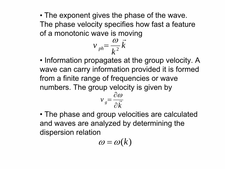
• The exponent gives the phase of the wave. The phase velocity specifies how fast a feature of a monotonic wave is moving

•

Information propagates at the group velocity. A wave can carry information provided it is formed from a finite range of frequencies or wave numbers. The group velocity is given by

•

The phase and group velocities are calculated and waves are analyzed by determining the dispersion relation

kk

v ph

r2

ω=

kv g r

∂∂

=ω

)(kωω =

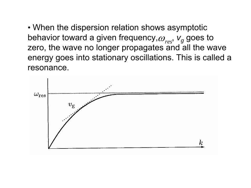
• When the dispersion relation shows asymptotic behavior toward a given frequency, , vg goes to zero, the wave no longer propagates and all the wave energy goes into stationary oscillations. This is called a resonance.

resω

•

MHD waves -

natural wave modes of a

magnetized fluid

–

Sound waves in a fluid

•

Longitudinal compressional oscillations which propagate

at

•

and is comparable to the thermal speed.

21

21

⎟⎟⎠

⎞⎜⎜⎝

⎛=⎟⎟

⎠

⎞⎜⎜⎝

⎛∂∂

=ρ

γρ

ppcs

21

⎥⎦

⎤⎢⎣

⎡⎟⎠⎞

⎜⎝⎛=

mkTcs γ

–

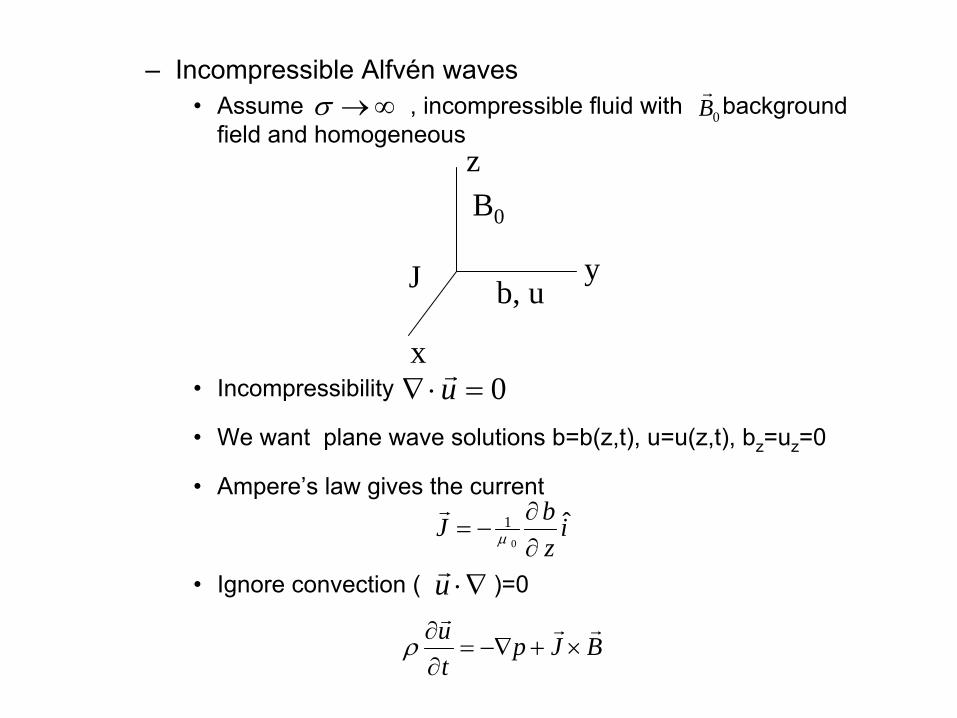
Incompressible Alfvén waves•

Assume , incompressible fluid with background field and homogeneous

•

Incompressibility

•

We want plane wave solutions b=b(z,t), u=u(z,t), bz

=uz

=0

•

Ampere’s law gives the current

•

Ignore convection ( )=0

∞→σ 0Br

z

y

x

B0

J b, u

0=⋅∇ ur

izbJ ˆ

0

1

∂∂

−= μ

r

∇⋅ur

BJptu rrr

×+−∇=∂∂ρ

•

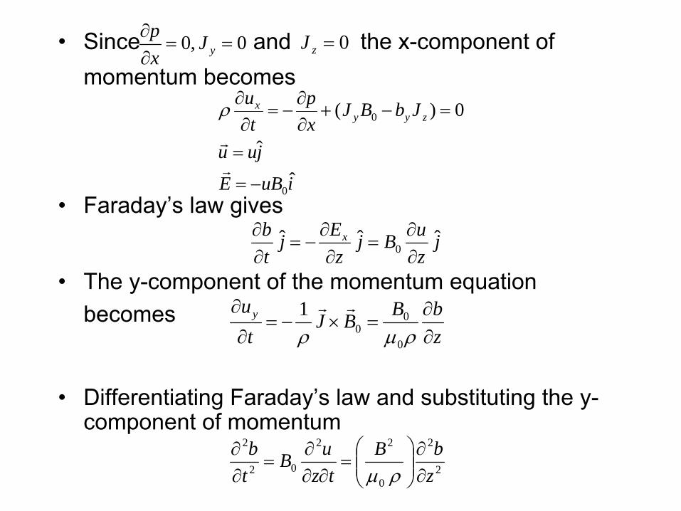
Since and the x-component of momentum becomes

•

Faraday’s law gives

•

The y-component of the momentum equation becomes

•

Differentiating Faraday’s law and substituting the y- component of momentum

0,0 ==∂∂

yJxp 0=zJ

iuBE

juu

JbBJxp

tu

zyyx

ˆ

ˆ

0)(

0

0

−=

=

=−+∂∂

−=∂

∂

r

r

ρ

jzuBj

zEj

tb x ˆˆˆ

0 ∂∂

=∂

∂−=

∂∂

zbBBJ

tuy

∂∂

=×−=∂

∂

ρμρ 0

00

1 rr

2

2

0

22

02

2

zbB

tzuB

tb

∂∂

⎟⎟⎠

⎞⎜⎜⎝

⎛=

∂∂∂

=∂∂

ρμ

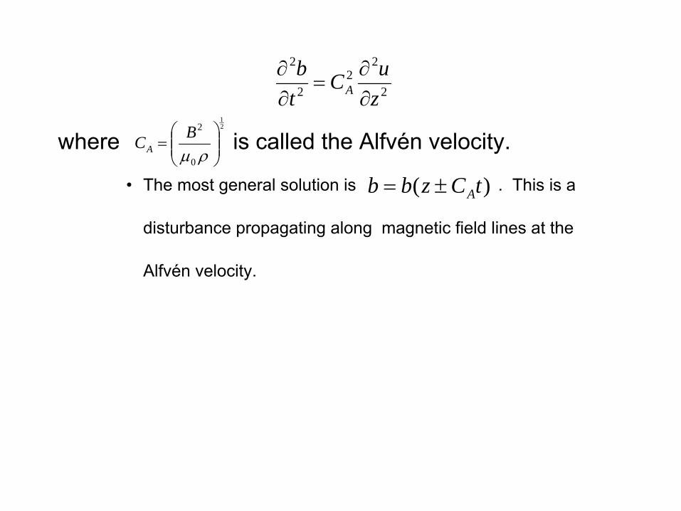
where is called the Alfvén velocity.

•

The most general solution is . This is a

disturbance propagating along magnetic field lines at the

Alfvén velocity.

2

22

2

2

zuC

tb

A ∂∂

=∂∂

21

0

2

⎟⎟⎠

⎞⎜⎜⎝

⎛=

ρμBCA

)( tCzbb A±=

•

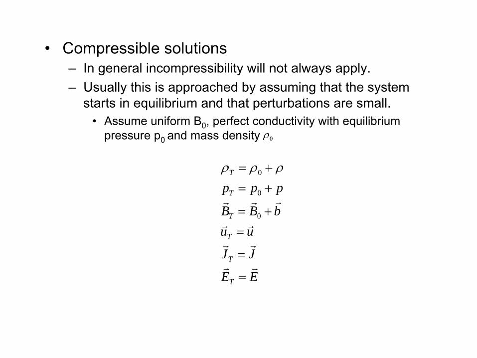
Compressible solutions–

In general incompressibility will not always apply.–

Usually this is approached by assuming that the system starts in equilibrium and that perturbations are small.

•

Assume uniform B0

, perfect conductivity with equilibrium pressure p0 and mass density 0ρ

EE

JJ

uubBB

ppp

T

T

T

T

T

T

rr

rr

rr

rrr

=

=

=+=

+=+=

0

0

0 ρρρ

–

Continuity

–

Momentum

–

Equation of state

–

Differentiate the momentum equation in time, use Faraday’s law and the ideal MHD condition

where

)(0 ut

r⋅∇−=

∂∂ ρρ

))((10

00 bBp

tu rrr

×∇×−−∇=∂∂

μρ

ρρρ

∇=∇∂∂

=∇ 20)( sCpp

0)))((()(

)()(

22

2

0

=××∇×∇×+⋅∇∇−∂∂

××∇=×∇−=∂∂

AAs CuCuCtu

BuEtb

rrrrr

rrrr

21

0 )( ρμ

BAC

rr=

0BuErrr

×−=

–

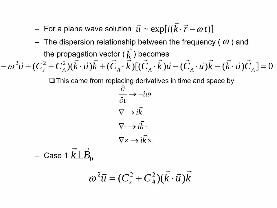
For a plane wave solution

–

The dispersion relationship between the frequency ( ) and the propagation vector ( ) becomes

This came from replacing derivatives in time and space by

–

Case 1

)](exp[~ trkiu ω−⋅rrr

ωkr

0])()())[(())(( 222 =⋅−⋅−⋅⋅+⋅++− AAAAAs CukkuCukCkCkukCCurrrrrrrrrrrrrrrω

×→∇×

⋅→∇⋅

→∇

−→∂∂

ki

ki

ki

it

r

r

r

ω

0Bkrr

⊥

kukCCu As

rrrr ))(( 222 ⋅+=ω

•

The fluid velocity must be along and perpendicular to

•

These are magnetosonic

waves–

Case 2

•

A longitudinal mode with with dispersion relationship(sound waves)

•

A transverse mode with and (Alfvén waves)

kr

0Br

kr

ur0Br

21

)()( 22Asph CCkkv +±== ωr

0Bkrr

0)()1)(()( 222222 =⋅−+− AAAsA CuCkCCuCkrrrrω

kurr

sCk ±=ω

0=⋅uk rrAC

k±=

ω

• Alfven

waves propagate parallel to the magnetic field.

•The tension force acts as the restoring force.

•The fluctuating quantities are the electromagnetic field and the current density.

–

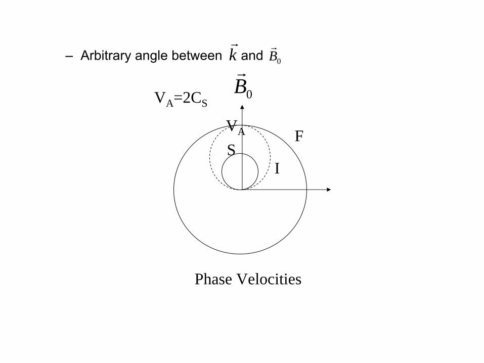
Arbitrary angle between and kr

0Br

0Br

F

ISVA

Phase Velocities

VA =2CS