instrumental effects as seen by a data analyst -...

Instrumental Effects as seen by a Data Analyst

Gabi Laske

IGPP, Seismometry Seminar, Feb. 19, 2002;DRAFT

Disclaimer

For this talk, I represent the ordinary data analyst who sends requests to a ”data management center” (DMC). Irepresent the data analyst (or end-user) who, often blindly, uses what is conveniently provided, often not knowingjust how much it takes to get a ground motion from out there in the field all the way onto my computer screen.I will show the bad things in a seismogram, not the good things. Naturally, I will point fingers and highlightbloopers that are happening to my fellow colleagues at ”network operations” (NO) and the DMCs. Nobody isperfect and bloopers happen but it is impolite to point at other peoples’ bloopers in public. So,to whom it mayconcern: I apologize! Writing this summary of my talk, I also realize that some issues need a few additionalremarks that I omitted in the talk by either forgetting to mention them, running out of time or being distracted bythe recording camera. I will therefore include these remarks as footnotes.1

Data Availability and Selection

”The good must be put in the dish, the bad you may eat if you wish”

In this section, I discuss issues of data return. I would like to get an idea of how many data actually make it fromthe field into my publications. A network never runs at 100%, e.g. some stations fail to return continuous data.2

Even though a station may produce nearly continuous data which are shipped by NO to the DMC, these datamay not be suitable for a particular study. Probably the most restrictive demands on high–quality seismogramscome from free–oscillation studies. Such studies typically require, among other things, 1) recordings fromobservatory–quality instruments, 2) continuous data over several days and 3) a high signal-to-noise ratio overthis entire period. To assess data availability, I have gone through my database which includes records for 37large earthquakes between 1986 and 2001. This database includes all records that are (or were) available atvarious DMCs (these include the IRIS-DMC, GEOSCOPE, sometimes in–house IDA, and lately GEOFON andthe Northern California Earthquake Data Center). Prior to an analysis, we go through all records interactivelyand edit them (e.g. remove ”easy” spikes; flag short, gravely noisy sections in otherwise high-SNR records). Wealso decide whether a record is to bedeleted(e.g. because of lack of data or lack of seismic signal) or shouldbeunloaded, i.e. put on hold because it cannot be used in a free oscillation study but in some other study. Forexample, a typical free oscillation study requires record lengths of more than 50h (more than 80h when high–Qinner–core sensitive modes are examined). A moment tensor (MT) determination on the other hand, which Iusually do for all great earthquakes, requires only 10h-long records.

1 I should mention that I myself have been in the field many times to deployment temporary seismic sites, mainlyin my former life as a travel–hungry student. So it is entirely possible that similar bloopers that created otherpeople’s nightmares have been caused by me.

2 Possibilities of failure range from a failing sensor, failing electronic equipment, to failing data recording, and/orNO processing, or even a faulty ”transmission” between NO and DMC.

1

Figure 1 shows histograms of ”data fitness” for some of the 37 events (some are omitted because of spacelimitations).

0

30

60

90

120

150analyzeunloaddelete

010000999898979696969695959494949493929190898786

Individual Datasets Fit for Normal Mode Studies

Figure 1 (data-columns.eps)

The total number of records has increased steadily until the mid-late 1990’s. Of course, the number of availabledigitial recordings was much less for times before 1985 (typically 25 suitable records per event). I should addthat our database includes old IDA (ID) as well as all global seismic networks (AS, SR, DW, HG, GT, IU, II,G, GE) and some regional networks (CD/IC, TS, MN, and lately BK and GE). The year 1993 approximatelymarks the time when the old networks were slowly phased out (e.g. ID, SR) or modernized and new GSN sitesstarted to become available. A slight decline in Figure 1 at the end of the 1990ies is due to the fact that somenetworks (e.g. MN, GE) were not available at the time of my requests and I have not yet gone back to re-requestthe missing data. In the last few years, the total number of records (as well as the ”unloads”) increased. This isbecause my requests include TS (and now BK) who had been operating STS-1 and STS-2 in the past. Recently,TS joined TRINET and requests to the DMC are responded to by automatically providing all of the CI records(mostly STS-2 and CMG-3T), a lot of which are weeded out3.

The fraction of discarded records depends somewhat on the earthquake. For example smaller ones are likely toproduce less useful records. Overall, the fraction of discarded records is quite stable though. Of the 37 eventsI have looked at, 28 events happened between July 1993 (the ”upgrade year”) and June 2001. I calculate the”typical data return rate” by averaging the histograms for these 28 events. The corresponding pie chart is shownin Figure 2. The fraction of data fit for a mode analysis can vary between 60 and 85% and is 73% on average.Considering that the ”up-time” of a network may typically be 80%, this implies that only 58% of the groundmotion that is supposed to be recorded in the field make it into my papers. This is, perhaps, a suprisingly lownumber.

Just to provide a quick idea of what category ”delete” and ”unload” seismograms look like, here are someexamples. I start with records from the great Arequipa earthquake on June 23, 2001, which is said to be thelargest earthquake recorded within the last 30 years. Figure 3 shows a category ”delete” seismogram4.

3 There are some nice records though, e.g. PLM, even though this has an STS-24 I start with II seismograms because these were the first available to me, thanks to Pete, and not because only II

has bad examples!

2

analyze

unload

delete

Average Dataset Fit for Normal Mode Studies

73%

12%

15%

Figure 2 (data-pie.eps)

Arequipa Event (Jun 23, 2001) at COCO

Time after Event [h]

Figure 3 (seis.coco.eps) A category ”delete” seismogram.

Obviously, this seismogram has sections of missing data that are too large to make the record useful for anystudy. This kind of data sparseness can be found in any network, not just II! Other examples for category ”delete”seismograms are those with no obvious seismic signal (e.g. records of ”bit noise”) and when ”spikes” of any kindare larger than the seismic signal and occur too often to be ”edited out”.

Figure 4 shows an example for a category ”unload” seismogram. The first 4 hours of this seismogram have agood SNR (so this part could be used for a MT study), but then big spiky signals make the following 5 h uselessfor an analysis. As I said before, the June 23, 2001 Arequipa Earthquake in Southern Peru is the largest recentearthquake so the spikes shown here are huge! We also have to remind ourselves that gaps in the data alter thestructure of a spectrum. Usually, small gaps in the data can be modelled in single record analyses. For example,to measure mode frequencies we can compare the spectrum of such a record with that of a synthetic one whosegap structure is identical to that in the data. Data gaps of the size shown here however, are very difficult to dealwith, especially if they occur near the front end of the record. Due to their different gap structure, such records cannot be used in stacking procedures, such as our techniques to calculate singlet and receiver strips. The particular

3

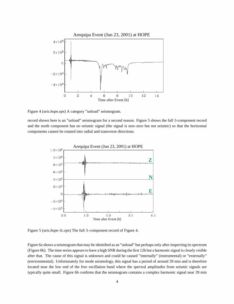
Arequipa Event (Jun 23, 2001) at HOPE


Figure 4 (seis.hope.eps) A category ”unload” seismogram.

record shown here is an ”unload” seismogram for a second reason. Figure 5 shows the full 3-component recordand the north component has no seismic signal (the signal is non–zero but not seismic) so that the horizontalcomponents cannot be rotated into radial and transverse directions.


Arequipa Event (Jun 23, 2001) at HOPE

Z

N

E

Figure 5 (seis.hope-3c.eps) The full 3–component record of Figure 4.

Figure 6a shows a seismogram that may be identified as an ”unload” but perhaps only after inspecting its spectrum(Figure 6b). The time series appears to have a high SNR during the first 12h but a harmonic signal is clearly visibleafter that. The cause of this signal is unknown and could be caused ”internally” (instrumental) or ”externally”(environmental). Unfortunately for mode seismology, this signal has a period of around 39 min and is thereforelocated near the low end of the free oscillation band where the spectral amplitudes from seismic signals aretypically quite small. Figure 6b confirms that the seismogram contains a complex harmonic signal near 39 min

4

~39min

Arequipa Event (Jun 23, 2001) at SNAA


Figure 6a (seis.snaa-all.eps) A potential category ”unload” seismogram...

Arequipa Event (Jun 23, 2001) at SNAA

Frequency [mHz]

fundamental

higher harmonic

Figure 6b (spec.snaa.eps)... and its spectrum.

plus its first harmonic. This signal dwarfs the fundamental mode spectrum of the great Arequipa earthquake andwe unload this time series (note though that the spectrum may be ok beyond about 2 mHz).

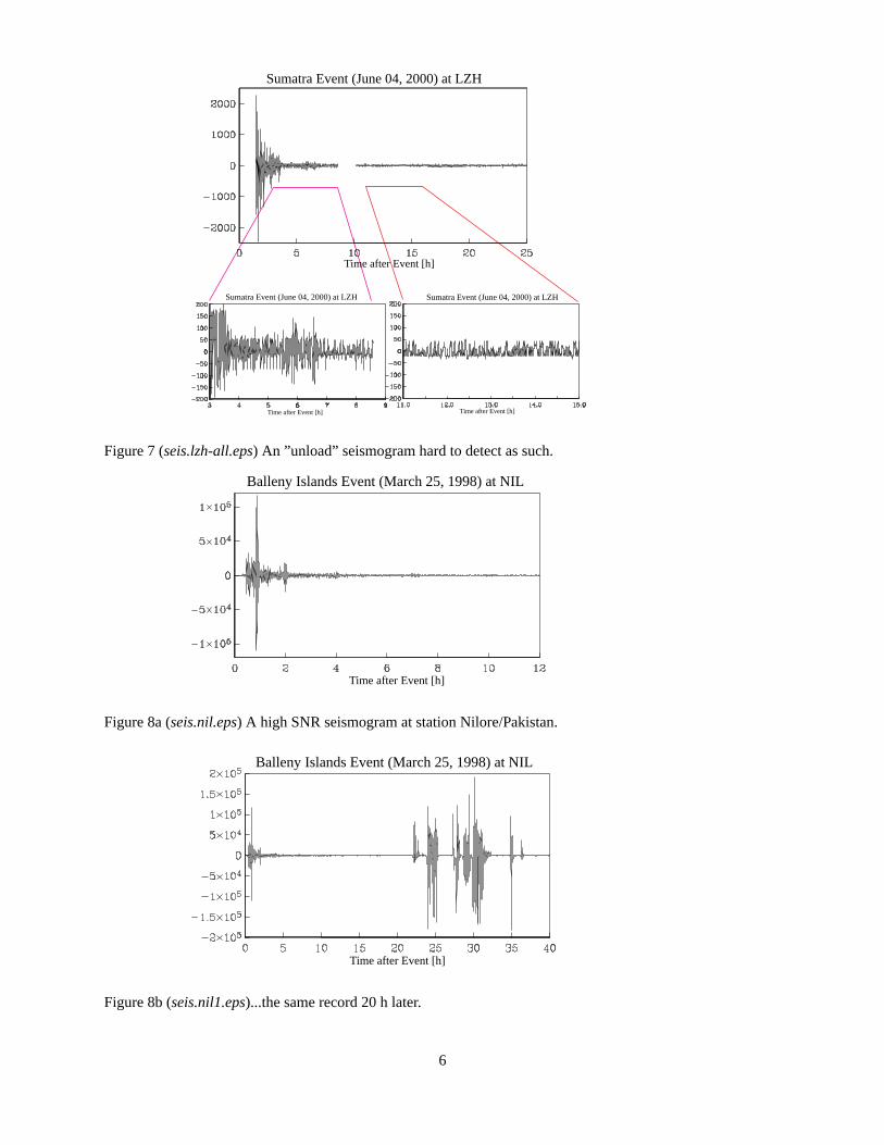
A tricky record that may pass as a ”to be analyzed” if not visually inspected is the one in Figure 7. The recordlooks noisy but ”normal” after automatic filtering. Of course, we do not have to be trained extraordinarily wellto find that the negative values in the later parts of the time series are set to ”zero”. I am sure that NO expertscan tell you immediately what instrumental defects can cause this type of phenomenon as well as the two-sided”comb-like” structure in the first part of the time series. I as the end-user can only say: ”unload”.

Jeanne next door has to endure quite a few screams of disappointment from me. The next example shows why thishappens. When you do this business for a while, you develop a ”personal relationship” with some of these sites.For one reason or another, they seem notorious for producing faulty records. So every time when an earthquakehappens, you anxiously sift through the new files and you want so badly that this one site has a really nice record,just this one time! Such a station is NIL (Nilore/Pakistan)5. And for the Balleny Islands Event in 1998, thisstation produced a beautiful record (Figure 8a).

... for about 20h. What then happened ... nobody really knows (Figure 8b). The Balleny Islands event also

5 NEVER name a station NIL!

5

Sumatra Event (June 04, 2000) at LZH



Time after Event [h] Time after Event [h]


Figure 7 (seis.lzh-all.eps) An ”unload” seismogram hard to detect as such.

Balleny Islands Event (March 25, 1998) at NIL


Figure 8a (seis.nil.eps) A high SNR seismogram at station Nilore/Pakistan.

Balleny Islands Event (March 25, 1998) at NIL


Figure 8b (seis.nil1.eps)...the same record 20 h later.

6

was a huge earthquake, but the spikes beginning about 23h after the earthquake, which get only worse as timegoes on (not shown here), dwarf the seismic signal6. I should mention that this particular record is a borderline”unload”. For some mode studies (e.g. high–frequency modes), 23h is close to Q-cycles of a mode which is theideal record-length for this mode to be analyzed. For cases like NIL we typically keep the record in the databasebut flag everything after 23h. Our analysis algorithms then check for the amount of available data and decide ifthis is enough for a particular mode or not. I should also add that NIL has produced fine records in the past thatare suitable for an MT study (only 10 h needed).

Figure 9 shows a quite annoying feature in a seismogram that is operator induced and needs to be edited beforethe filtering and removal of the instrument response (we need time series of ground acceleration).

Bolivia Event (June 09, 1994) at BOSA


Figure 9 (seis.boli-bosa-all.eps) Calibration pulses at GTSN stations.

The little pulses that, to my knowledge, may or may not show up on a regular basis, are calibration pulses thatare now pretty much unique to the GTSN network (GTSN, or GT, is run by AFTAC). The greatness of the 1994Bolivia Earthquake emphasizes just how huge these calibration pulses can be. These pulses are a nighmare todeal with because no matter how you filter the time series before you remove the instrument response, thesepulses always seem to be larger after this process. We usually end up flaging such pulses but we have to remindourselves once again that this procedure alters the character of the spectrum. Luckily, the pulse shown here ispretty much the largest I have found during my quick search for an example before my talk. However, the dangerof these pulses lies in the possibility that I don’t detect them during the editing process of my database when theyoccur early in the time series. In such cases they are likely hidden in the seismic signal but significantly alter thespectrum.7

6 We do not know exactly what causes these spikes but we know that the problem is the sensor. Only the verticalcomponent of the KS54000 seems to be doing these funny things and the problem is almost impossible to trackdown. You go through all the effort to take the sensor out; no spikes. You put the sensor back in; spikes.... Thesensor will finally be replaced in the near future. In the meantime, only the data of the horizontal components areshipped to the DMC; Pete Davis, personal communication.

7 Guy and Bob Woodward actually wrote a paper on how to model these calibration pulses for the old SRO stations(AS, SR). SRO used to have these pulses irregularly, then once a day and then once every 5th day after Guycomplained to NO. I have not gone through ”my” calibration pulses systematically so I have no feel for these

7

Kuril Islands Event (Oct 04, 1994) at ENH


Figure 10 (seis.nonlin-enh.eps) A non–linear instrument response to a large R1 wave train.

The next figure (Figure 10) shows another instrument–induced problem in a time series. This is a relatively oldrecording on an instrument of the CDSN network that has recently been upgraded with the help of IRIS. Thepicture shows the instrument’s non-linear response (with its typical long-period relaxation) to a very large R1surface wave train. The Kuril Islands earthquake was only about 20 degrees away and was actually greater thanthe great Bolivia earthquake that happened earlier in the same year. Back in 1994, ENH had a 16-bit dataloggerand its dynamic range was obviously not large enough to allow for the linear recording of strong seismic. signals7a

In saying this, I simply assume that the sensor itself can handle such motion. I should add that this non-linearityin the seismogram does not affect my mode studies, since I typically start at least 1h after the event time.8

Time after Event [min]5 7 9 1131

Kashmir Event (Nov 19, 1996) at AAK.KN

Time after Event [min]5 7 9 1131

Kashmir Event (Nov 19, 1996) at ULHL.KN

Figure 11 (seis.kashmir-kn.eps) Telemetry dropouts at a regional array.

The last example of records that cause my occasional screams leads us away from free–oscillation studies into thedomain of surface wave studies. In these, I often use records from temporary or semi–temporary networks. Being

things and ”edit them out”.7a Actually, Guy remarks that the feedback loop is the problem and not the 16-bit datalogger and I assume that he’s

right.8 ENH has an STS-1 and was an excellent producer of high-quality free-oscillation spectra. This site was ”upgraded”

in September 1997, presumably with a ”better” datalogger (the sensor remained) and has sadly produced second-rate spectra ever since.

8

at IGPP, of course my first choice of such networks are Frank’s. Figure 11 shows the 1996 Kashmir earthquake(Ms=7.1,∆=800 km) at two KNET stations. The intermediate–period Rayleigh wave is clearly coming in. Thisis the waveform immediately after the hole for AAK but the long periods are probably spread out across the hole.I cannot use these records for a dispersion analysis, for obvious reasons. The holes in the time series are causedby telemetry dropouts that happened during the earlier days of Frank’s networks.9

STS-1 or STS-2”... that is the question!”

This seminar was arranged for several reasons. We all know that we are running out of observatory-qualityseismometers. The STS-1 are no longer built and the KS54000 probably not either10. The question arises of whatshould we do in case there is no ’next generation’ observatory–quality sensor within the near future. Could wedo with the next best thing (STS-2/CMG-3T)? This question is difficult to address but does need to be discussed.If we want to records ultra–low frequency free oscillation, we likely cannot replace the STS-1 with STS-2s andthe fear is that the retirement of our last STS-1 will coincide with the ultimate great earthquake that we have beenwaiting for for 40 years (unlikely but possible).

In Figure 12, I show you what a collection of spectra should look like. The spectra on the left hand side are 11 ofthe 14 spectra of the GEOSCOPE global seismic network that were available to me immediately after the greatArequipa Earthquake last June. This earthquake was big enough to excite the gravest free oscillations and mode

0S3 should easily be visible on the spectra. This is indeed the case for quite a few spectra but the majority of allspectra I have so far is too noisy for0S3 to have a high SNR. The GEOSCOPE spectra are actually exceptionallygood – though II also has exceptionally good spectra which I don’t show here (e.g. BFO, PFO and SUR). On someindividual spectra, we can even see the elusive0S2 (e.g. SSB, and also BFO.II) which has been seen for perhapsa handful earthquakes in the last 30 years. These are indeed observatory–quality spectra which I would like tosee much more often (and we should, given the magnitude of this earthquake and the quality of the instruments).We all know too well that the quality of a seismogram does not depend on the quality of an instrument alone,and that perhaps the environment plays the dominant role. The panel on the right hand side of Figure 12 is acollection of spectra that I received after a data request to the German GEOFON DMC. With the exception ofKMBO (a global GEOFON station near Nairobi) and ISP (a Mednet/GEOFON station in Turkey), the quality ofthese spectra is quite a bit poorer than that of the GEOSCOPE network. I’d like to draw your attention however tothe spectra with a red circle. Some of these have an excellent SNR down to about 0.5 mHz (e.g. IBBN, RGN, butalso WLF, and even PSZ). All these sites have STS-2 sensors and, in fact, should not have a spectrum like this.Figure 13 shows the velocity responses for SSB (the GEOSCOPE site having a STS-1) and RGN (the GRSN sitehaving a STS-2). The response for RGN rolls off much faster at low frequencies than that for SSB. Below 3mHz,the response of the STS-2 is less than that of the STS-1 by almost a factor 10 (compare RGN adjusted, which isshifted downward for better comparison).

I should say that none of the STS-2 sites are part of the global GEOFON network (e.g. RGN is a station ofthe German Regional Seismic Network) but are provided in response to a generic request to the DMC. These

9 I am not exactly sure I understand how these networks are run. Presumably, there is no recording medium involved,so nobody has to go and change tapes at each site. The signals are instead sent by radio to some recording center.Radio has hick–ups ... Gabi loses Rayleigh waves.

10 And, of course, Erhard is spending his sabbatical here, so what better time could we possibly have this seminar?

9

inu

atd

can

rer

scz

ssb

spb

ech

ppt

nouc

kip

0.20 0.40 0.60 0.80 1.00 1.20frequency [mHz]

0

0

0

0

0

0

0

0

0

0

0

0S2

0S3

0S4

1S2

0S0

0S5

1S3/

3

0S6

3S2

1S4

Arequipa Event (06/23/01) at G_(VHZ)

isp

malt

psz

rgn

kmbo

rue

eil

sfuc

trte

ibbn

wlf

kbs

0.20 0.40 0.60 0.80 1.00 1.20frequency [mHz]

0

0

0

0

0

0

0

0

0

0

0

0

0S2

0S3

0S4

1S2

0S0

0S5

1S3/

3

0S6

3S2

1S4

Arequipa Event (06/23/01) at GE(VHZ)

Figure 12 (specs.peru.eps) Observatory–quality ultra–low frequency free oscillation spectra

Velocity Instrument Response for SSB (STS-1) and RGN (STS-2)

SSBRGN

Am

plitu

de

Frequency [Hz]

RGN (adjusted)

Figure 13 (resps.ssb-rgn.eps)

spectra are truely spectacular and we know that, at some sites, they are consistently so. For example, RuediWidmer-Schnidrig used the spectra at RGN (among other GRSN spectra) to study the continuous free oscillationsof the Earth.11 The question arises of what makes these sites so special. Have the NOs done anything unusualto the installation to achieve such a high SNR? RGN (R¨ugen, Germany) is an island in the Baltic Sea and to my

11 Note however, that none of the STS-2 sites has a0S3 which is probably truely burried in the instrument noise.

10

knowledge, it is just a pile of sediments, as is the larger part of Northern Germany. Erhard Wielandt, who ispresent at this seminar, comments that this is a miracle that ”we do not understand”. There is nothing specialabout the installation, no special vault but just a ”hole in the ground”, with no special shielding12. To get to mypoint, it seems that though this is not the rule (plenty of experience with IU and CI/TS sites) in some cases, theSTS-2 produces spectacular free–oscillation spectra. We have numerous GSN sites, with either an STS-1 or aKS54000, that perform only poorly in the very-long period band. Some are identified as consistently bad, i.e. Ihave never seen a high-quality spectrum and there is no prospect of improvement13. These are often importantistallations for other purposes (e.g. CTBT sites or excellent body wave sites) and perhaps we should discusswhether the installation of an observatory quality sensor makes a lot of sense or whether a STS-2 would do andthe replaced STS-1 could be used at a ”better” site.

The Effects of Calibration ...

”... on Arrival Angles; Shear Wave Splitting ... and and and...”

I am probably expected to talk about sensor orientations and the like, so I’ll briefly recall how I ”detected” someof the horizontal component misalignment at GSN sites.

Figure 14 (seis.3-comp.eps) A typical 3–component surface wave seismogram.

Figure 14 shows a typical 3-component seismogram of the first two Rayleigh (R1, R2) and Love (G1, G2) wavetrains. On a laterally homogeneous Earth, Rayleigh waves are visible only on the Z and R components, whileLove waves are visible only on the T component. We see quite clearly a wave packet on the T component arrivingat the R1 arrival time. The fact that R2 and G2 do not show up on the ”wrong” component is strong evidence thata faulty component calibration cannot be the cause for the anomalous R1 signal (the signal of G1 on the Z andR components could be G1 but could also be Rayleigh wave overtones that arrive prior to R1). These waveformanomalies are due to lateral refraction of surface waves in a heterogeneous Earth, away from the source–receiver

12 My own conversation with Winfried Hanka, the executive director at GEOFON, revealed that RGN made use ofthe ”Wielandt-shielding”, though I do not know what this means. Winfried wrote a report on this for IRIS andthe online version is found at http://www.gfz-potsdam.de/geofon/manual

13 I will not mention these sites but I am happy to discuss these in private. Some of these sites are known to haveenvironmental noise problems for about 99% of the time that will likely remain.

11

4.9

4.854.85

4.8

4.75

4.7

4.65

4.6

4.55

Figure 15 (ray-map.eps. A true ray on a laterally heterogeneous Earth. The top panel shows the structure alongthe source–receiver great circle which has been rotated to be along the equator; the asterisk is the source, the dotis the receiver.

great circle. The wave packets then arrive at the recording station at an angle (see Figure 15 for the concept) whichcan be measured on the three-component seismogram, as function of wave type and frequency. Using a lineartheoretical framework, these data can be interpreted in terms of laterally heterogeneous structure, as function offrequency (i.e. a global phase velocity map). Before talking about problems, let’s first have a look at the data.For each station, I typically plot arrival angles in rose diagrams (see Figure 16 for the concept).

N

EW

Off-Great Circle Arrival Angles

S

0

30

-30

Rose Diagram

Figure 16 (pol.example.eps). Concept figure for the rose diagrams, in which I present my measured arrival angles.The left panel shows the coordinate system of a seismometer and back azimuths of three earthquakes (stars). Thedashed lines mark the ”measured” arrival direction for each of these earthquakes (the black lines mark the greatcircle direction). The right panel shows a rose diagram in which each arrival angle is plotted with respect to itsgreat circle direction (which is always the 0◦-line). In this presentation and scale, arrival angles range from -30to 30◦.

Figure 17 shows arrival angles for 6.4 mHz Love waves I measured at 4 GSN stations (PPT, NNA, AAK and PFO).The angles in a typical dataset vary between±10◦ and cluster around 0◦. Sometimes, the data cluster aroundother angles (e.g. around -5◦ at PPT). In principle, if the data coverage is azimuthally highly uneven, this ”shift inthe mean value” can be caused by structure. For well-sampling data, this is somewhat unlikely and more so if this

12

0

30

-30

PPT

0

30

-30

AAK 0

30

-30

PFO

0

30

-30

NNA

Love Waves at 6.4mHz

-5.78±0.61º 0.56±0.53º

-6.53±0.67º 0.08±0.37º

Figure 17 (pol.gsn.eps). Rose diagrams and ”Apparent North” for 4 GSN stations.

shift is seen at different frequencies and for both wave types that sample 3D structure very differently. There aretwo important issues I need to point out: 1) the signal in the arrival angle dataset is relatively small. Predictionsusing published phase velocity maps can be as high as 15◦ but are usually smaller than 5◦. 2) Arrival anglemeasurements depend strongly on instrument calibration and component misorientation. As far as instrumentaleffects are concerned, the most straight forward effect to account for is a component misorientation. We assumethat the calibration of both horizontal components is given accurately in the DATALESS SEED volumes at theDMC (the files we extract the instrument responses from). We further assume that both horizontal componentsare orthogonal. A misorientation at each station can then be included as additional unknown in a non-linear jointinversion for structure, where 2-3 iterations typically lead to convergence. To obtain the component misalignment,I perform such inversions for typically 3 frequencies for both wave types and then average the results. I elaborateon this because I think that my technique (perhaps in contrast to others) is probably the most reliable to distinguishbetween structural and instrumental effects. The numbers for my 4 example stations are given beneath the rosediagrams as ”Apparent North”. A negative value implies that the system is rotated clockwise with respect to true(geographic) North. Figure 17 implies that the components at stations PPT and AAK are significantly misoriented.This figure is somewhat historical as I, being a fresh postdoc at Scripps, showed it at the EGS 1994 meeting inGrenoble, France. This talk probably got the most feedback of all my talks ever, and I was instantly (in)famous,because I asserted that an observatory–quality station (PPT) was in error. Only now do I understand how bold Iwas back then. Amazingly enough, only a few months later, the NOs at GEOSCOPE confirmed that PPT was offby 5◦(pretty close to what I had predicted). An error was also confirmed at AAK though the misrotation therewas more complicated. The NOs checked the station and found that only the North component was misaligned(by 6◦) but not the East component. The fact that I predicted 6◦ is probably a coincidence (as I had assumedorthogonal components) but the point is that I was still able to detect orientation problems at this site.14

14 A question from Mark Zumberge prompts the discussion of whether my determinations of ”Apparent North” areaffected by calibration uncertainties, or in other words, how well does the calibration have to be known? Thisquestion is actually non-trivial to address. Calibration problems of individual horizontal components are probablynot easy to detect by my analysis. Back-of-the-envelope calculations show that if one of the two components isoff by a factor of two, individual arrival angles can be affected by as much as 20◦. This, of course, is much biggerthan the signal due to Earth structure. But the average around which the values cluster (and hence suggest amisrotation of the sensor package) may actually stay the same, depending on the azimuthal data coverage. So the

13

Figure 18 (sw-splitting.eps) A shear wave splitting study for the SAUDI data.

So how does a component misorientation affect science? Well, it does affect arrival angles but I think that I canaccount for this in my inversions. Other studies that are more sensitive to bias caused by such effects, because thereare typically only few measurements, are shear–wave splitting studies. These studies typically do not account forcomponent misalignment before interpreting shear–wave splitting in terms of seismic anisotropy (and ultimatelymantle flow within the Earth). Figure 18 shows an example for Saudi Arabia. This is a shear–wave splitting studydone for the Saudi Seismic Broadband Network that was operational from late 95 through early 97. The directionof fast shear–wave velocity is usually coherent across the array and approximately follows absolute plate motion.Two outliers are AFIF and SODA. I am not recalling the details of this publication but the temptation is great toiterate on why these two sites have different directions.

0

30

-30

AFIF 0

30

-30

SODA

0

30

-30

AFIF 0

30

-30

SODA

Love Waves at 15mHz

Rayleigh Waves at 15mHz

Figure 19 (pol.saudi.eps). Arrival angle data at two sites of the temporary Saudi Arabian Seismic BroadbandNetwork. Of the 8 sites, at least two have small but significant component misalignment: apparent North at AFIFis−4.22± 0.66◦ and at SODA is−2.72± 0.54◦.

This study was done about two years before I had the time to check the orientation of the sensors. Figure 19

trade–off may actually be quite small. If one of the two components is off by 10%, then the effects on individualarrival angles can still be as high as 3◦ (bad news for me) but probably won’t affect the mean (so my misrotationvalues are probably reliable estimates).

14

shows my data for both stations for Rayleigh and Love waves at 15 mHz. For the Saudi Array, I did my analysisat slightly higher frequencies because that array has STS-2 sensors and may be noisy at longer periods. Thedata seem to cluster at a small negative angle and my inversions confirm this. The misrotation is quite small andcan by no means account for all the anomalous signal in the shear–wave splitting study but the coincidence iscurious and speaks for itself. My friend Rob Mellors who installed the instruments confirmed that the magneticdeclination was about 2◦ and so a correction in the wrong direction might be embarrassing but conceivable15.

0

30-3

0

BLA

0

30

-30

BW06

0

30

-30

ISCO 0

30

-30

LBNH

0

30

-30

ELK

Love Waves at 10mHz

Figure 20a (pol.usnsn.eps) Arrival angle data at 5 USNSN stations.

My last example serves as a case study for the proposed USArray which will have a permanent component as wellas a large flexible array component (”Bigfoot”) both datasets of which I would be very interested in. A few yearsago, the IRIS DMC made the data of the USNSN easily available and these data are now part of our database.At the time when I analyzed these data, about 18 months worth of data were available, which is the expected lifetime of a USArray ”Bigfoot” site.

0

30

-30

0

30-3

0

10mHz Love Waves at ELK

Prior to 97.254 After 97.300

Figure 20b (pol.elk.eps) Time dependence of arrival angle data at station ELK.

15 I have yet to check if this goes in the right direction!

15

The USNSN has 28 sites for which I measured arrival angles (Figure 20 shows some examples) and my resultsare quite depressing. While some sites display the typical rose diagram (e.g. ISCO, LBNH), other sites clearlyhave orientation problems (BLA, BW06, ELK). The arrival angles at station BW06 are so extreme that I had tochange my computer code to be able to analyze this station. A particularly interesting, and difficult, site is ELKfor which the data seem to cluster around at least two different means. It turns out that the data prior to julianday 254 in 1997 cluster around a large positive value, while they cluster around a slightly negative value after day300. So, I have it black and white that somebody must have visited ELK in the fall of 1997 and done somethingto the installation. Actions like these are particularly devastating for an ”end user” since none of this is reportedby NO.

BLA 9.45 ± 0.82

BW06 -26.41 ± 0.62

CEH 9.72 ± 1.34

ELK 31.80 ± 0.71 before 97.254

GOGA 7.67 ± 0.97

MCWV 5.90 ± 1.20

MIAR 5.74 ± 1.19

WMOK -17.69 ± 1.03

WVOR -18.38 ± 0.90

Apparent North

-3.93 ± 0.56 after 97.300

9 of 28 more than 5 degrees4 of 28 more than 10 degrees

Figure 21 (pol.table.eps) Gross deviations of ”Apparent North” from true North at USNSN.

A summary of the orientation status of the USNSN is given in Figure 21. Nine out of 28 stations have anorientation error of more than 5◦. This is a third of the network! And four out of 28 station have an orientationerror of more that 10◦. This isunacceptablefor the proposed USArray16.

Dataloggers

or ”The Subleties in a Seismogram”

I had prepared this section for the talk but then cut it out because I ran out of time. This is about a subtle signal wehad detected in the data some time ago but didn’t know what its cause might be. It later turned out to be relatedto round-off problems in the filtering process of the II network’s Mark7 datalogger. The problem has recentlybeen detected conclusively when the Mark8 datalogger had a test run at PFO and the Harvard group noticed thatthe noise level of the Mark7 datastream was higher than that of the Mark8 datastream.

Figure 22a shows the great Balleny Islands earthquake in 1998 recorded that the Black Forest Observatory, BFO.This is a beautiful record for free oscillation studies for which the very small event about 100h after the BallenyIsland event is neglected (or edited out) (this is a Ms=5.6 earthquake on Mar29 north of Ascension Islands,53◦ away from BFO). Ruedi Widmer-Schnidrig noticed for this event, as for others, that wave forms of suchsmall events sometimes look ”peculiar” on the VH data stream, with a long–period signal at the back–end of the

16 Duncan Agnew remarks that the numbers that occur suspiciously often are close to 15 and 30◦. 15◦ is close tothe declination within the U.S., so one has to wonder ....

16

Balleny Islands Event (March 25, 1998) at BFO




Figure 22a (mark7.eps) The Balleny Islands Earthquake recorded at BFO with a high SNR.



Figure 22b (seis.ball2-bfo.eps). The first Rayleigh wave train of the Balleny Islands earthquake on the VH datastream of BFO. The signal is ”on scale” and shows no non-linearities.

Rayleigh wave train. This looks suspiciously like a non-linear instrument effect. Of course, this doesn’t makesense, if we remind ourselves that the much larger Balleny event did not show such a signal (Figure 22b).

Pete and I discussed what the cause for such a long–period signal might be and to me this waveform lookedactually quite normal. Depending on the size of the earthquake, on how the seismogram is filtered and on theEarth structure the wave is travelling through, the long-period Rayleigh wave may very well arrive at the backend of the wave train. I tested this with synthetic seismograms and a comparison was inconclusive (i.e. I wasbasically right).

A disturbing fact however was that the waveforms of the VH channel and the LH channel looked different (Figure22c). It looked like the VH channel was missing some of the high–frequency content at the back-end of thewave trains. This was very disturbing and pointed toward a problem with the datalogger, after we had ruled outany problems with filtering on our computers17. The great difficulty of this problem to pin down was that such

17 Though this should not be the case, it is remotely possible that my filtering of the LH channel did not removeenough of the short-period signal to compare it to the VH data. The purpose of my figure is to illustrate what wesaw in the data, and not to quantify the effects.

17



LHZVHZ

Figure 22c (seis.ball4-bfo.eps).

waveforms were sort of transient. They did not occur on ALL Mark7 recordings but they did seem to occurprimarily on II records. Perhaps this only occurred at particular stations and consistantly so, which I do not recall.It turned out that indeed only small signals were affected and occurred primarily when the original data streamhad a significant DC offset. The problem was a round–off error in the filtering from the original 100 Hz data downto BH, LH and VH channels. The VH channel was the worst affected since it underwent the most (imprecise)filtering. The NOs have succeeded in reconstructing the signals as they should have looked like and are currentlyreplacing the faulty records at the DMC. It is not really clear just how much of my research is affected by this. Ipersonally do not look at such small events on the VH channels and it is not clear to me how much a dispersionmeasurement is affected by this filtering error (though amplitude/attenuation research might be another story, asare noise studies).

Timing Problems

”a thing of the past?”

During this seminar series, we have been discussing the issue of timing several times and we repeatedly agreedthat timing ”is not a problem anymore” in the era of GPS. We also agreed, however, that there are still rare,isolated cases, e.g. when the GPS receiver loses the signal and the internal clock starts to run freely. A questionthat needs to be discussed in our ”What’s next” session is what should we do in these cases. Should we let theclock run freely and record the time with a second clock so that data analysts have a chance to take care of it orshould the NOs resynchronize the time (I vote for the latter)? The questions I will address today: Are there anytiming problems nowadays? Can we detect them? How severe are these timing problems? And what effects dothese have on our research?

How do we know that a station has timing problems? We all know that this is a tough question to address. If wepick a travel time and compare it to a prediction using a model, then measured time differences can have manycauses. Foremost among these are 3D structure (what we want to know), source location errors, errors in thedata analysis (e.g. picking inaccuracies), interference effects from other seismic (or whatever) signals, and lastlyinstrumental effects (the one we are talking about here). Instrumental timing errors of only a few seconds cannotbe detected in a raw dataset. A reliable way to detect timing errors is to compare co–located instruments. Thereis no such case that two independent observatory quality instruments occupy the same site18 but there are two

18 though an increasing amount of GSN sites have secondary sensors, presumably with their own datalogger

18

PFO (Pinon Flat, CA); LHZ channel; residuals II-TS

Time

Res

idua

l [s]

PFO (Pinon Flat, CA); LHZ channel; residuals II-TS

Time

Res

idua

l [s]

Figure 23 (timing.pfo.eps). The relative timing between the II and TS dataloggers at PFO.

GSN sites that have two dataloggers connected to the same sensor, PFO and KIP. After removing instrumentaleffects, the times picked from the two data streams at each site should be identical.

G

IU

KIP (Kipapa, Hawaii); LHZ channel; residuals G-IU

Time

Res

idua

l [s]

KIP (Kipapa, Hawaii); LHZ channel; residuals G-IU

Res

idua

l [s]

Time

Figure 24 (timing.kip.eps). The relative timing between the G and IU dataloggers at KIP.

The figures I will show you come from Guy’s body wave travel time work. Figure 23 shows the differences ofP travel times picked at the two LHZ data streams at station PFO (one is from the II data logger, the other onefrom TS). There was a temporary problem with the TS response in the DATALESS SEED volume at the DMCthe data for which are omitted here. A significant difference of about 13 s occurred in the middle of 1993 for ashort time (successive days are consistent). I can’t tell you right now which of the two dataloggers is at fault herebut it would be obvious if we checked Guy’s list. Apart from this we notice an almost constant offset betweenthe two data streams of about 0.4 s where the TS stream is delayed. The travel time picking accuracy is 0.1-0.2 sso this difference is just resolvable. We do not know the cause of this but we can say that the two dataloggershave a time difference of about 0.4 s.

At station KIP (Kipapa, Hawaii), a similar setup exists with a GEOSCOPE datalogger and a IU datalogger hookedup to a STS-1 (Figure 24). There the difference between the timing of the two dataloggers is much larger. For

19

some time in 1992, the GEOSCOPE timing was advanced by 1 min, and later by about 20 sec19. Apart fromother gross excursions (and I don’t recall which data stream has the timing error), there is also a constant offsetbetween G and IU for the years 1990 through 1994. We find that, in this case, the IU data stream is late by 1 s.The cause of 1 s timing errors are manifold. I know from experience in field experiments, that some systemssynchronize to the next higher second, so can be off by a second. I don’t know if observatory quality systemshave the same problem but I guess it is conceivable. Another timing problem of the order of 1 s is thehandlingof leap seconds. I am told that they occur quite often and that different NOs handle these in different ways.

ANMO (Albuquerque, NM); LHZ channel; IU

P R

esid

ual [

s]

Time

Figure 25 (timing.anmo.eps). Absolute timing errors at station ANMO.

Unfortunately (or fortunately!), PFO and KIP are the only sites where two data loggers are hooked up to thesame sensor so we cannot perform similar comparisons for other sites20. On the other hand, we are indeed ableto get an idea of the timing from the absolute body wave picks. Figure 25 shows the absolute time residuals atstation ANMO. For this figure, travel times have been calculated for a 3D earth and subtracted from the measuredtime21. The residuals shown in this figure are due to timing errors at the station, if the trends in Figure 25 areidentical to the trends found for correspondingS picks (not shown). Anything not identical cannot be due totiming, unless there is a differential timing between the 3 components of the instrument (theP picks come from avertical components, while theS picks come from a transverse component). Figure 25 suggests 1 s timing errorsat ANMO for a short while in 1982, 1987 and 1993 and about 2 s timing errors in 1990 and 1997. As mentionedbefore timing problems in mutliples of 1 s are, unfortunately, probably very common.

How relevant is a timing error of 1 s? Figure 26 shows typical histograms forP andS travel time residuals relativeto PREM. Any deviation from 0 s is regarded as due to 3D structure (in our inversions, we actually do allow forsome of this signal to come from earthquake location errors). The signal in theP dataset is much smaller than intheS dataset. The variance in theP dataset is about 1 s (marked by the purple bar), i.e. much of the signal of the3D Earth is only of the order of 1 s (or smaller)! The table on the right hand side summarizes this. The signal inS from 3D structure is larger than that from earthquake mislocation and noise (picking errors, timing errors etc)

19 I can confirm this with my independent mode study. I analyzed a Fiji Islands earthquake occurring on July 11(julian day 193). I had the GEOSCOPE and IU VHZ components and, in addition, the old IDA gravimeter(ID.VGZ). Since I am using data sampled at 40 s, my determinations are much less precise than Guy’s butI obtained a difference between VGZ and IU.VHZ of -4 s and between G.VHZ and IU.VHZ of -61 s whichconfirms Guy’s value.

20 Though Frank Vernon points out that we could compare GSN data streams to his own, e.g. PFO and AAK.21 the actual procedure is a little more elaborate but the details are irrelevant for this talk

20

Typical Body Wave Residuals

Data Location 3D Structure Noise (LP)

Set σx σ3D σN

P 0.9 1.0 0.9S 2.0 3.0 1.3

* (mis) location effect important for P!

Contributions to the Standard Deviation of a TypicalSummary Ray in the Body Wave Datasets

(in seconds)

Figure 26 (timing.body.eps). Typical body wave travel time anomalies and their causes.

but all these signals are of the same size forP ! Hence, 1 s timing errors are really not acceptable and we need tostrive to do better than this.

shifted by 38 samples: 25min 20 s

Sumatra Event (June 04, 2000) at KONO


Sumatra Event (June 04, 2000) at KONO


Figure 28 (timing.kono.eps). Data (black) and synthetic seismograms (red) for the great 2000 Sumatra Earthquake,before and after shifting the synthetic.

In one of his recent papers, Guy listed gross timing errors (5 s or more) in a table (Figure 27). Note that the timingerrors at stations ATD, ENH, GNI, PAS and SBA occur in 1994 and are therefore to be regarded ”recent”. You maywonder if such gross timing errors were common 8 years ago but not today. Figure 28 shows a recent timing error

21

Station Time interval

ANMO 1985/150–1985/157ANTO 1992/90–1994/187ATD 1994/243–1994/298BNG 1992/311–1993/122CCM* 1993/99–1993/110CHTO 1978/184–1978/217COL* 1993/20–1993/264COR 1990/55–1990/74CRZF 1989/232–1989/256ENH 1994/205–1994/289GDH 1992/195–1992/237GNI 1994/46–1994/51; 1994/100–1994/366GRFO 1989/162–1990/347HIA 1987/118–1987/129; 1987/145–1987/158HRV 1988/53–1988/70HYB 1989/203–1989/302INU 1990/203–1990/222; 1992/2–1992/73KEV 1982/246–1982/249; 1986/120–1986/143KIPb 1992/161–1992/272KMI 1987/118–1987/129MBO 1991/292–1993/79MAJO 1985/282–1985/296PAS* 1988/103–1988/143; 1988/282–1988/293;

1992/13–1992/20; 1994/281RER 1991/361–1992/58SBA 1994/266–1994/366SCP 1984/264–1985/83; 1987/327–1988/69;

1988/258–1988/297; 1988/359–1989/26SNZO 1983/277–1983/304; 1992/181–1992/242;

1992/326–1993/74TAU 1988/183–1988/209; 1992/274–1992/344;

1993/265–1993/289TUC* 1992/166–1992/252ZOBO 1985/110–1985/135; 1993/252–1993/264

Table 1. Intervals of erratic timing deduced from the analysis of the temporal behaviorof S and P residuals through the end of 1994. The dates are inclusive, e.g. for ZOBO allpicks from 1985/110 up to and including 1985/135 have been deleted. Entries markedby an asterisk are assumed to be exact 1 minute timing errors (or multiples thereof) andhave been corrected. The entry for KIP refers to the GEOSCOPE data stream. Notethat start and end days correspond to days when we have measurements and so may notexactly reflect the duration of the timing problem.

Figure 27 (table1.eps).

that Guy would have never found because it wouldn’t have fit on his screen. I calculated synthetic seismogramsfor the great Sumatra earthquake on June04, 2000. The synthetic record at station KONO is significantly delayed(the data record has the first Rayleigh wave train missing). The two time series need a relative shift of 25 min20 s to be aligned so it is clear that KONO has a truely spectacular timing error of 25 min (give or take 20 s–as Isaid earlier, I cannot pin down timing errors that accurately)!!

One concluding remark of this section is in order. We need to talk about the ”time dependence of timing errors”.”We” (actually Guy) had realized quite some time ago, that G and IU had, at certain times, a timing differenceof pretty much exactly 0.5 s (which was corrected before making Figure 24). Contacting both NOs, we receivedtwo ascertainments that the ”other” datalogger was at fault. It later turned out that it was the GEOSCOPE loggerand if you request data of this period nowadays, you may find that both streams are actually in phase. What

22

happened in this case is that GEOSCOPE corrected their timing a posteriori. This post–processing phenomenonis not network dependent and could happen to any station. This does not appear to be such a big deal but theimplication of this is absolutelyhuge! For example, let say I requested a data stream of the June 1994 Boliviaearthquake at station ANMO in July 1994 and found a timing error of 120 s (just an assumption!). I then warn mycolleague G¨oran Ekstr¨om at Harvard who has requested the same data in 2000. He may ask me if my computercodes are working right, because he finds no timing error at ANMO for June 9, 1994. You know why: the timingerror has been fixed at the DMC in the meantime. This brings us back to Guy’s table. He invested tremendouseffort and time to detect and report these timing errors but only 3 years down from now, his table may not matchwith the data then stored at the DMC. Depressing, isn’t it? So what should we do abut this problem? There isthe suggestion that we should not touch the data but provide accurate ”station histories” at the DMCs (I thinkI would endorse this idea). This leaves the really blind data analysts who have never heard of station histories(unfortunately probably the majority of us) in the dark. Some say that the data should be corrected. This wouldcause the ”expert” data analysts (such as Guy) who typically store large databasesmajor headaches. I cannotcount how often we refurbished our database with updated requests to the DMC and initially unknowingly mixedun-corrected and corrected data. The rectification of this mix-up costs us a huge amount of valuable time.

Our Friends at the Data Managment Centers

This section I had also prepared for the talk but omitted due to time constraints. I do find it important however topoint out that a data enduser does not only have to worry about ”instrumental effects” created on the way betweenthe seismic site and NO. A data enduser also has to deal with ”instrumental effects” that are created after the dataleft NO. The latter may only learn about this when the DMC sends (seemingly unjustified) complaint about astation or time period to NO.

Let me briefly review the usual path of ground motion from the field onto my computer screen, from the enduser’spoint of view:

- ground motion is recorded by instrument in some format

- record is shipped to NO

- NO checks record and decides whether it’s worthy of distributing

- NO puts this record into a SEED file and sends it to the DMC

- Gabi sends breqfast request to DMC

- DMC assembles ”Gabi’s” SEED file from data stored on jukebox

- Gabi ftps her SEED file from DMC disk onto her own

- Gabi uses RDSEED (provided by DMC) to read the SEED file and converts record into own format(from SEED to SAC to GFS format)

- Gabi edits raw time series on screen

- Gabi extracts instrument response from SEED or DATALESS SEED volume using EVALRESP(provided by DMC) and corrects time series

- Gabi plots time series on screen and analyzes it

And here trouble usually starts for the data analyst. I’ve been looking at global seismic data provided by the DMCfor about 10 years now (I looked at BFO and GEOSCOPE data for much longer than that). During this time I’vesurvived about a ga-zillion software upgrades at the DMC, each single one of which caused some disturbancein my data processing. Some of the changes are really minor and easy to fix but can cost the data analyst an

23

Z,1

N,2

E,3

left-handed coordinate system

right-handed coordinate system

Z,1

N,2

E,1

motion positive motion negative

Figure 29 (dip.definition.eps). The definition of the dip in different coordinate systems.

disproportional amount of time.

For example, one of the early ”upgrades” of RDSEED was to provide the option of automatic polarity checksand of flipping records as they are read out. Some instruments have true polarity-flips (e.g. ERM.II) which needto be corrected. A major headache, however, was to combine data from different networks. A fundamental issueto agree upon is the coordinate system in which a seismic motion is recorded (Figure 29). We all know thatthe coordinate system is ZNE but there is, amazingly enough, a disagreement over what Z actually is, i.e. whatis positive. The coordinate system in seismology has positive Z going up (in this case ZNE is a left–handedcoordinate system). Unfortunately, it is conventional to use a right–handed coordinate system and in this case, Zis going down. Choose NOs out of each of these two groups and the confusion about the sign of the dip of Z isperfect. Of course, the actual motion recorded by the instrument is always the same but the definition of the dipnow becomes NO-dependent. I don’t remember exactly who was using what but, just for the record, GEOSCOPEused touse a different convention (the same as old IDA/ID) than everybody else. Having the polarity check inRDSEED switched on, this routine would then flip all GEOSCOPE data during the reading process, which wasexactly the wrong thing to do because now all vertical motion in the GEOSCOPE records had the wrong sign. Soin the busy days when Guy, Junho, Harold and I myself had their fingers (and their own heads) involved in thereading process, our database was a huge mess. I think, in the meantime, ID ”died out” and GEOSCOPE waspersuaded to change their convention so we all seem to be consistent now.22

Another ”problem” is that the folks at the DMC (have to) strive to make RDSEED become more universal. Forexample, recent versions are supposed to be used for GSN and PASSCAL data alike. A consequence of theseupgrades is that the input parameter list constantly changes. I never use RDSEED in interactive screen mode butin c-shell script files (batch mode) and I don’t have to say more. The lifetime of my c-shell script files is far lessthan various versions of Microsoft Windows.

A very sad and actually quite grave issue is ”data aging”. This should not happen but great seismograms thatwere available at the DMC only a few years ago get lost. I started free oscillation studies relatively late, after myfellow postdoc Junho Um had left. This was several years after the 1994 Bolivia earthquake the data collectionfor which I was not involved in. When I joined in, the raw data were no longer on disk available and it was onlyapproximately known what was done to the data that are stored in the database. Trying to be consistent with

22 ... and the red blobs in our models really are red and not blue!

24

Bolivia Event (Jun 09, 1994) at NOU

Time [h]

Frequency [mHz]

Figure 30 (seis.boli-nou.eps) A historical record: the seismogram at NOU is no longer available at the DMC.

BOCO LHE 1996.006

read with RDSEED 4.15read with RDSEED 4.17

Figure 31 (rdseed.boco.eps). A SEED file read with different versions of RDSEED.

the data processing, I started from scratch and re-requesting the data from the DMCs. This exercise was quitesobering. Some records (I do not recall which ones these were) now had huge holes while the old ”processed”data on Guy’s disk were continuous. This implies that parts of seismograms were lost between 1994 and 1999,within only 5 years! Figure 30 shows a record (and its spectrum) that is historical, meaning that it is no longeravailable. My requests to the DMC does not return any data for station NOU. This spectrum is one of the 10 bestwe have for the Bolivia earthquake!

25

Another sad and grave story is that SEED files and various versions of RDSEED become incompatible and datapractically unrecoverable. Figure 31 shows an example of this. At some point during the past few years, wedecided to refurbish our database. We requested several years worth of data at the DMC read them with theSEED reader and put them on a big disk. The data could (and still can) then be used by whoever needs them.In summer of 2000, I decided to look at data recorded in North America and had a look at our LH database. Inoticed that, in a certain time interval, seismograms at BOCO didn’t look right (red trace). This also happenedfor other stations, at other times. Sometimes it happens that a SEED file gets corrupted due to a disk error on ourdisk or an undetected error during ftp from the DMC to us. So in order to track this problem down, I re-orderedthe data from the DMC. The new SEED file however had the same problem, so we knew that the original SEEDfile did not ”age” on our disks. During the reading process, I got an error message:

Steim 2 Decompression Sample Count Error. Expected 1808, counted 1600. Lost values will bePadded with Zeroes.

I then realized accidentally that the DMC was providing an updated version of RDSEED. Reading the SEED filewith the new update (version 4.17 instead of 4.15) gave the blue trace in Figure 31. Obviously the ”new” SEEDfiles were not down–ward compatible and this change was made without our knowledge. We are supposedly ona user-email list at the DMC but we never receive emails about software upgrades and the DMC web site alsodoes not announce updates (perhaps somewhere 20,000 levels down but I could not find it). I don’t have to tellyou that it cost us major time to debug our database, a problem we had repeatedly pointed out to the DMC.

Figure 32 (usnsn.timing.eps) A timing error introduced by RDSEED.

The non–communication between the DMC and endusers is a really big problem. I seem to be one of the fewwho actually does provide feedback to the DMC and with an odd smirk in their face they now refer to me as ”nother again”. My colleague G¨oran Ekstr¨om also is one of the bugging kind. About two days before the last FallAGU meeting, he asked me whether I found any timing problems with the USNSN data....two days before AGU!

26

Since I had only looked at long period surface wave data, I was not in the position to say anything conclusive.He sent me a figure (Figure 32) that contained enough material to panic. Using his own SEED reader, G¨orangot a different time series for USNSN data than when using the latest version of RDSEED (4.18) (distributedby the DMC). The DMC reader seemed to have put in extra samples, delaying the following data stream by 1 s.The source of the error was identified during a lengthy search and discussion process. Data are stored in datablocks, and a request to the DMC usually spans several of these data blocks. NO at USNSN write the data blocksin a slightly non–standard way. Successive data blocks begin with the sample that the last data block ends withand RDSEED interprets this as being two separate data points, duplicating the one datum when data blocks arestrung together. We do not know how often this occurs in our database but this incidence prompts yet anothermajor refurbishing process. If these duplications occur more often than once per event I can redo about 10,000hand–picked dispersion measurements.

shifted by 4 samples: 160 s

Arequipa Event (June 23, 2001) at BFO



Arequipa Event (June 23, 2001) at BFO

Figure 33 (evalresp.eps). A timing error introduced by EVALRESP.

RDSEED is not the only software that potentially alters data. I spent a good part of my last summer to helpthe DMC debugging EVALRESP. The cause of all trouble was the great Arequipa earthquake in June. For”interesting” earthquakes I routinely gather all VH data I can get a hold of to determine a source mechanism.There are some interesting cases when the USGS publishes a mechanism that is very different from the Harvardquick CMT. More than once, I also got a different MT that was very close to a later revision of the HarvardCMT. We usually update instrument responses from the DATALESS SEED volumes only once a year so forthese ”special events” I read the responses from the new SEED files. The Arequipa event quickly turned into amajor headache when many of my synthetic seismograms were shifted relative to the data by large amounts. Anexample is shown in Figure 33 where the synthetic has to be shifted by almost 3 minutes (!) to match the data.We initially assumed that complicated source processes (e.g. a long source duration) could be the cause of this.The fact that not all records were shifted led to wild speculations about never before seen directivity effects, untilI noticed that this time shift was network dependent. IU stations had no shift, GEOSCOPE stations were 120 soff, II stations 160 s and BK stations even more. The mistake I made here was that I made certain that I used

27

the latest versions of RDSEED and EVALRESP. Had I used an old version of EVALRESP, I would have had noproblems. The communication with the DMC was lengthy and frustrating but we finally identified several bugsin EVALRESP (v.3.2.18). Just to give you a flavor of the types of things that happened, a beta version duringthe debugging process would run fine on a PC at the DMC and under CDE on my Sun Ultra 5 but not underOpenWindows. Such incidences usually prompt my correspondents to conclude that the fault is to be sought onmy end and not theirs, which of course is not the case. The debugging process at the DMC ended with the releaseof version 3.2.19 and the conclusion that this can only be a preliminary fix. The ultimate culprits, according toour friends at the DMC, were the NOs. The problem is that different NOs use a header parameter called ”groupdelay” in different ways, or not at all, and older versions simply ignored this (which was correct in most cases forGSN). Version 3.2.18 reads this group delay23 and puts it into the responses. I cannot stress often enough thatthe DMCs (especially the IRIS DMC) needs to work on improving the communication with all NOs (not just IU)and endusers.

Surface Waves and the Ocean Bottom

”... to boldly go ...”

With this section, I want to give you an outlook of where I would like to go with my research on regional scale.One of the reasons why we have this seminar is to discuss global seismometry which faces an uncertain future,because the STS-1 are no longer built. But regional seismology also harbors issues that are yet to be resolved.

17s28s37s

50s

70s

Sensitivity to SV

Dep

th [

km]

20

60

40

80

100

140

160

180

120

Figure 34 (swell.kernels.eps). Sensitivity of Rayleigh wavaes to structure at depth.

One of many things I would like to know before I retire is how the Hawaiian hotspot works. To find this out, weneed a nice tomographic image of the lithosphere–asthenosphere system of the Hawaiian Swell which can onlybe achieved by using OBSs. The standard body wave tomography provides a fairly good picture of the deeperupper mantle (i.e. between 200 and 600 km, depending on the aperture of the recording array). For example,the ICEMELT experiment illuminated the deeper Iceland Plume. To image the upper 200 km however, we need

23 that it shouldn’t read, because all NO except IU do not seem to be knowing about this ... Some NOalso don’t know about the software upgrades and use the same version of EVALRESP as we do or evenolder...COMMUNICATION!

28

either regional seismicity or surface waves. Figure 34 shows how Rayleigh waves sample shear velocity withdepth, as function of period. Only 70 s Rayleigh waves have significant sensitivity to structure below 140 km andare necessary to reliably resolve structure below 80 km. It is therefore essential to measure dispersion at theseperiods and longer. Here exactly lies the problem for an ”OBS” experiment.

10-4

10-3

10-2

10-1

100

101

10-20

10-18

10-16

10-14

10-12

10-10

10-8

ASL Upper Bound

ASL Lower Bound

Buried BBOBS

Surface BBOBS

MELT - Webb

KIP

Standard OBS

Episensor Instrument Noise

Borehole

Figure 35 (swell.all-resp.eps) Ambient noise curves at OSN-1 (by Vernon and Orcutt).

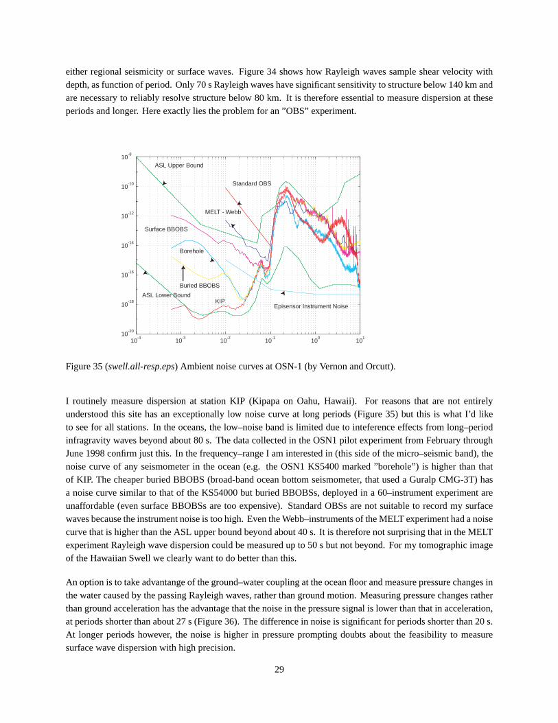
I routinely measure dispersion at station KIP (Kipapa on Oahu, Hawaii). For reasons that are not entirelyunderstood this site has an exceptionally low noise curve at long periods (Figure 35) but this is what I’d liketo see for all stations. In the oceans, the low–noise band is limited due to inteference effects from long–periodinfragravity waves beyond about 80 s. The data collected in the OSN1 pilot experiment from February throughJune 1998 confirm just this. In the frequency–range I am interested in (this side of the micro–seismic band), thenoise curve of any seismometer in the ocean (e.g. the OSN1 KS5400 marked ”borehole”) is higher than thatof KIP. The cheaper buried BBOBS (broad-band ocean bottom seismometer, that used a Guralp CMG-3T) hasa noise curve similar to that of the KS54000 but buried BBOBSs, deployed in a 60–instrument experiment areunaffordable (even surface BBOBSs are too expensive). Standard OBSs are not suitable to record my surfacewaves because the instrument noise is too high. Even the Webb–instruments of the MELT experiment had a noisecurve that is higher than the ASL upper bound beyond about 40 s. It is therefore not surprising that in the MELTexperiment Rayleigh wave dispersion could be measured up to 50 s but not beyond. For my tomographic imageof the Hawaiian Swell we clearly want to do better than this.

An option is to take advantange of the ground–water coupling at the ocean floor and measure pressure changes inthe water caused by the passing Rayleigh waves, rather than ground motion. Measuring pressure changes ratherthan ground acceleration has the advantage that the noise in the pressure signal is lower than that in acceleration,at periods shorter than about 27 s (Figure 36). The difference in noise is significant for periods shorter than 20 s.At longer periods however, the noise is higher in pressure prompting doubts about the feasibility to measuresurface wave dispersion with high precision.

29

Figure 36 (swell.acc-press.eps) Acceleration and pressure noise in 1 km depth, off CA coast (by Webb, 1998).

Figure 37 (swell.dp-resp.eps) Impulse response of the SWELL L–CHEAPO instruments (using a DPG sensor).

In our SWELL pilot exeriment near Hawaii in 1997/1998 we therefore wanted to investigate just this. The impulseresponses of our L–CHEAPOs had not been measured before but had instead been taken from spec sheets as formost OBS studies the instrument response is a minor issue. I initially didn’t make friends in our OBS team withmy persistent inquiries about the responses but they made our engineer Paul Zimmer sufficiently nervous. Hesat down with our student Harm van Avendonk and performed a calibration test. This exercise probably savedmy experiment because it turned out that the responses were nowhere near what we expected them to be. Paulchanged a few resistors (this is magic to me) and managed to expand the response to the period range I wasinterested in (and we had initially thought we had) (Figure 37).

So thanks to Paul Zimmer, Cris Hollinshead, Dave Willoughby and numerous cruise helpers, we collected textbookwaveforms (Figures 38 and 39) and I could measure dispersion in an unprecedented period range (sometimesbetween 17 and 90 s!). A closer look at the record section however reveals one trace as being rather noisy (trace7). In fact, it is so noisy that the S arrival cannot be made out. This brings us to the implied title of my talk,”instrumental effects which inhibit my analyses”. Trace 7 suffers from harmonic noise that we observed quiteoften at the SWELL instruments but that was previously unknown to us because these instruments never beforerecorded long–period seismic signals. The noise was confined to a very narrow frequency band (Figure 40) andwe could usually also see the first 2 harmonics.

30

Figure 38 (swell.lcheapo.eps) An L–CHEAPO during deployment in the SWELL experiment.

Rat Islands Dec17 (351), 97; 04:38:53.0h0=33km; Ms=6.5

bp:0.015-0.05Hz

Epi

cent

ral D

ista

nce

[deg

]

aligned on 50s Rayleigh Waves

Figure 39 (swell.seismogram.eps) An earthquake recorded at the SWELL pilot array. For comparison, the traceat nearby GSN station KIP is also shown.

The properties of this noise were quite interesting. It was different at each site and extremely intermittent andappeared to be very rare at the deep sites. Figure 41 shows the time–dependence at site 2 for the first few daysof operation. The instrument was in the water for about two hours or so and recorded a small earthquake (theblue horizontal streak at time 106, 20:00 – the other blue streaks every 6h are put in by me to mark the timeand are not in the time series!).After the earthquake, this station was very quiet for about a day and 6 h, thenthe harmonic noise started and lasted for about 6 h before it stopped and picked up after another 14 h (day 108),

31

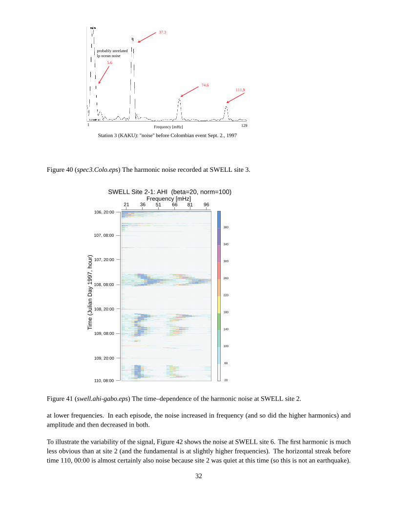
Station 3 (KAKU): ''noise'' before Colombian event Sept. 2., 1997

Frequency [mHz]1 129

37.3

74.6111.9

5.6

probably unrelatedlp ocean noise

Figure 40 (spec3.Colo.eps) The harmonic noise recorded at SWELL site 3.

SWELL Site 2-1: AHI (beta=20, norm=100)

20

60

100

140

180

220

260

300

340

380

Frequency [mHz]21 51 8136 66 96

Tim

e (J

ulia

n D

ay 1

997,

hou

r)

106, 20:00

107, 08:00

107, 20:00

108, 08:00

108, 20:00

109, 08:00

109, 20:00

110, 08:00

Figure 41 (swell.ahi-gabo.eps) The time–dependence of the harmonic noise at SWELL site 2.

at lower frequencies. In each episode, the noise increased in frequency (and so did the higher harmonics) andamplitude and then decreased in both.

To illustrate the variability of the signal, Figure 42 shows the noise at SWELL site 6. The first harmonic is muchless obvious than at site 2 (and the fundamental is at slightly higher frequencies). The horizontal streak beforetime 110, 00:00 is almost certainly also noise because site 2 was quiet at this time (so this is not an earthquake).

32

20

60

100

140

180

220

260

300

340

380

SWELL Site 6-1: ONAGA (beta=20, norm=100)Frequency [mHz]

21 51 8136 66 96

Tim

e (J

ulia

n D

ay 1

997,

hou

r)110, 00:00

110, 12:00

111, 00:00

111, 12:00

112, 00:00

112, 12:00

113, 00:00

Figure 42 (swell.onag-gabo.eps) The time–dependence of the harmonic noise at SWELL site 6.

N&F 4-20Myr

N&F 52-110Myr

N&F >110 Myr

N&F 20-52Myr

leg 34

leg 18

Measured and Predicted Phase Velocities for Two Legs

x xx

x

xx x

xx

x x

x Priestley andTilmann, 1999

Figure 43 (swell.disps.eps) Two interstation dispersion curves measured at the SWELL pilot array. Leg 18 wasclose to Big Island on the Swell, while leg 34 was in the deep ocean off the Swell.

The horizontal streak at time 111, 12:00 is a large earthquake in the Santa Cruz Islands region to the southwest.

That this noise could potentially affect my dispersion measurements is evident in Figure 43 which shows inter–station dispersion curves. The little bump in the leg–18 dispersion curve near 45 s is unphysical and could have

33

been caused by the contamination from harmonic noise (though other causes are possible). I have not gone backto verify this for every dispersion curve and I also don’t really know what would be the best way to correct forthis. Since this is a pilot experiment, I decided to let the results be as ”raw” as possible.

Possible Scenarios

1) 2)

3) 4)

Loihi

T REMO RS

TID

ES

RE

HT

AE

W

cu rrents currents

damped forced oscillator

phase lock loop

125Hz

2KHz

CHOPPER

1mHz

misalignment

beating

giant squid... still a possibilityunhappy electronics

Figure 44 (swell.scenarios.eps) Possible Scenarios for the harmonic noise at the SWELL pilot array.

The search for the possible origin of the harmonic noise was quite an entertaining exercise. Of course, the firstguess was seismic signals. Unfortunately, the widely favored cause by tremors from the Hawaiian volcanoes hadto be ruled out quickly because the signal was so different between stations. It was curious however, that thedeepest site off the Swell seemed to have been the quietest. Since the instrument package was more than 3 mlong, it was conceivable that deep–ocean currents could force oscillations on the package. But only very fewpeople warmed up to this theory. Spahr Webb suggested internal problems in the instrument package, i.e. that theclock driving the sensor could beat with the clock driving the electronics if they were not synchronized. This wasidentified by John Orcutt as a grave mistake (”never put two clocks into one instrument”) and the new generationLC2000 now has only one clock. Well, if we go out again with the new instruments, and we still record the noise,then we have to search for other reasons.

Food for Thoughts

I would like to conclude this talk with one last issue that we may want to discuss in our final ”what’s next” sessionin March. The SWELL pilot experiment was regarded in the community as only partially successful, which Itake personal but cannot do much about. The reason for this is, oddly enough, that we recorded the waveformson pressure sensors and not on existing seismometers. I already discussed the reasons why we did not go outwith the currently available OBSs. Had we done so, I would not have the high–quality dispersion curves I havetoday. Going out with pressure sensors however, so my proposal reviewers say, has the disadvantage that werecord only Rayleigh waves and these with only one component. With pressure sensors, we cannot record theparticle motion of surface waves, which also carries useful constraints on the structure along the source–receiverray path. Neither can we record Love waves which provide complementary resolution of structure at depth. To

34

my knowledge, only two Love waves have ever been recorded with current OBSs. One was a large regional eventduring the MELT experiment (less than 20◦ away). The other one was the 1999 Hector Mine earthquake recordedon Leroy Dorman’s OBSs off Costa Rica, also only about 20◦ away. I would say that these are the most expensiveLove wave records we have and we have to remind ourselves that surface wave dispersion of relatively largeearthquakes recorded at a distance less than 20◦ are very difficult to analyse. The trade-offs of this (increasinglypolitical) issue are obvious. We proved with our pilot study that we are able to obtain Rayleigh wave dispersioncurves with our L-CHEAPOs in an unprecedented period range. The full period range is essential to resolvestructure reliably at depths below 80 km. Proposal reviewers are reluctant to recommend funding of DPG seismicexperiments because of the highly specialized approach of using Rayleigh waves in passive seismic experimentson the ocean floor (no matter how successful SWELL pilot was). Using only DPGs, we cannot measure shear–wave splitting and receiver functions, the standard observables which are much more widely (over)interpretedthan surface waves. Neither can we measure particle motion or Love waves. Current OBSs are probably goodenough to measure shear–wave splitting but the sensors that record both Rayleigh and Love waves in a usefulperiod range probably have yet to be built. As a surface wave seismologist interested to obtain a tomographicimage of the Hawaiian Swell, I would rather have an excellent collection of wide–band Rayleigh waves than amediocre (short–period) one and one additional Love wave, but my proposals would not get funded if I expressedthis. In return, I cannot really regard a proposal that promises to resolve structure at 150 km with 50 s Rayleighwaves as fundable, so we are sort of stuck in the review process. The OBS community needs a seismic sensorthat is capable of giving us both excellent Rayleigh and Love waves though I am personally a little sceptical aboutrecording Love waves in the oceans with a high SNR. In the meantime, while we are waiting for the ultimatesensor to appear on the horizon, I will not go out to sea without a DPG and the equipment being fine–tuned torecord long periods.

Acknowledgments.This talk was a contribution to our ”Seismometry” seminar which was held during ErhardWielandt’s sabbatical visit to IGPP.

35

instrumental effects as seen by a data analyst -...

Documents