introduction to computing at sio: notes for fall class, 2018shearer/comp233/main.pdf · 2.nedit...
TRANSCRIPT

Introduction to Computing at SIO:
Notes for Fall class, 2018
Peter ShearerScripps Institution of OceanographyUniversity of California, San Diego
September 24, 2018

ii

Contents
1 Introduction 11.1 Scientific Computing at SIO . . . . . . . . . . . . . . . . . . . . . . . 2
1.1.1 Hardware . . . . . . . . . . . . . . . . . . . . . . . . . . . . . 21.1.2 Software . . . . . . . . . . . . . . . . . . . . . . . . . . . . . . 2
1.2 Why you should learn a “real” language . . . . . . . . . . . . . . . . 31.3 Learning to program . . . . . . . . . . . . . . . . . . . . . . . . . . . 41.4 FORTRAN vs. C . . . . . . . . . . . . . . . . . . . . . . . . . . . . . 51.5 Python . . . . . . . . . . . . . . . . . . . . . . . . . . . . . . . . . . 6
2 UNIX introduction 72.1 Getting started . . . . . . . . . . . . . . . . . . . . . . . . . . . . . . 72.2 Basic commands . . . . . . . . . . . . . . . . . . . . . . . . . . . . . 92.3 Files and editing . . . . . . . . . . . . . . . . . . . . . . . . . . . . . 122.4 Basic commands, continued . . . . . . . . . . . . . . . . . . . . . . . 14
2.4.1 Wildcards . . . . . . . . . . . . . . . . . . . . . . . . . . . . . 152.4.2 The .bashrc and .bash profile files . . . . . . . . . . . . . . . 16
2.5 Scripts . . . . . . . . . . . . . . . . . . . . . . . . . . . . . . . . . . . 182.6 File transfer and compression . . . . . . . . . . . . . . . . . . . . . . 21
2.6.1 FTP command . . . . . . . . . . . . . . . . . . . . . . . . . . 212.6.2 File compression . . . . . . . . . . . . . . . . . . . . . . . . . 222.6.3 Using the tar command . . . . . . . . . . . . . . . . . . . . . 232.6.4 Remote logins and job control . . . . . . . . . . . . . . . . . . 24
2.7 Miscellaneous commands . . . . . . . . . . . . . . . . . . . . . . . . . 262.7.1 Common sense . . . . . . . . . . . . . . . . . . . . . . . . . . 28
2.8 Advanced UNIX . . . . . . . . . . . . . . . . . . . . . . . . . . . . . 282.8.1 Some sed and awk examples . . . . . . . . . . . . . . . . . . . 30
2.9 Example of UNIX script to process data . . . . . . . . . . . . . . . . 312.10 Common UNIX command summary . . . . . . . . . . . . . . . . . . 35
3 A GMT Tutorial 373.0.1 Setting default values . . . . . . . . . . . . . . . . . . . . . . 52
4 LaTeX 534.1 A simple example . . . . . . . . . . . . . . . . . . . . . . . . . . . . . 544.2 Example with equations . . . . . . . . . . . . . . . . . . . . . . . . . 554.3 Changing the default parameters . . . . . . . . . . . . . . . . . . . . 57
4.3.1 Font size . . . . . . . . . . . . . . . . . . . . . . . . . . . . . . 574.3.2 Font attributes . . . . . . . . . . . . . . . . . . . . . . . . . . 574.3.3 Line spacing . . . . . . . . . . . . . . . . . . . . . . . . . . . 58
iii

iv CONTENTS
4.4 Including graphics . . . . . . . . . . . . . . . . . . . . . . . . . . . . 594.5 Want to know more? . . . . . . . . . . . . . . . . . . . . . . . . . . . 61
5 Fortran 635.1 Fortran history . . . . . . . . . . . . . . . . . . . . . . . . . . . . . . 645.2 Texts and manuals . . . . . . . . . . . . . . . . . . . . . . . . . . . . 645.3 Compiling and running F90 programs . . . . . . . . . . . . . . . . . 65
5.3.1 The first program explained . . . . . . . . . . . . . . . . . . . 665.3.2 How to multiply two integers . . . . . . . . . . . . . . . . . . 67
5.4 Why you should always use ‘implicit none’ . . . . . . . . . . . . . . 695.4.1 Alternate coding options . . . . . . . . . . . . . . . . . . . . . 70
5.5 Making a formatted trig table using a do loop . . . . . . . . . . . . . 715.5.1 Fortran mathematical functions . . . . . . . . . . . . . . . . . 745.5.2 Possible integer vs. real problems . . . . . . . . . . . . . . . . 745.5.3 More about formats . . . . . . . . . . . . . . . . . . . . . . . 75
5.6 Input using the keyboard . . . . . . . . . . . . . . . . . . . . . . . . 765.7 If statements . . . . . . . . . . . . . . . . . . . . . . . . . . . . . . . 77
5.7.1 If, then, else constructs . . . . . . . . . . . . . . . . . . . . . 795.8 Greatest common factor example . . . . . . . . . . . . . . . . . . . . 805.9 User defined functions and subroutines . . . . . . . . . . . . . . . . . 81
5.9.1 Subroutines . . . . . . . . . . . . . . . . . . . . . . . . . . . . 835.9.2 Linking to subroutines during compilation . . . . . . . . . . . 85
5.10 Internal procedures . . . . . . . . . . . . . . . . . . . . . . . . . . . . 875.11 Extended precision . . . . . . . . . . . . . . . . . . . . . . . . . . . . 89
5.11.1 Integer sizes . . . . . . . . . . . . . . . . . . . . . . . . . . . . 935.12 Arrays . . . . . . . . . . . . . . . . . . . . . . . . . . . . . . . . . . . 94
5.12.1 Program to check user input for day of month . . . . . . . . . 955.12.2 Program to compute prime numbers . . . . . . . . . . . . . . 965.12.3 Checking for problems with the -fcheck=bounds option . . . 1005.12.4 More about random numbers . . . . . . . . . . . . . . . . . . 1025.12.5 Arrays as subroutine arguments . . . . . . . . . . . . . . . . . 103
5.13 Character strings . . . . . . . . . . . . . . . . . . . . . . . . . . . . . 1035.14 I/O with files . . . . . . . . . . . . . . . . . . . . . . . . . . . . . . . 1075.15 More about multi-dimensional arrays . . . . . . . . . . . . . . . . . . 111
5.15.1 Arrays of strings . . . . . . . . . . . . . . . . . . . . . . . . . 1145.16 A more complex example of data processing . . . . . . . . . . . . . . 1145.17 Example sorting routine from Numerical Recipes . . . . . . . . . . . 1195.18 Example of saving values in a subroutine . . . . . . . . . . . . . . . . 1215.19 Complex numbers . . . . . . . . . . . . . . . . . . . . . . . . . . . . 1255.20 Array operations in F90 . . . . . . . . . . . . . . . . . . . . . . . . . 127
5.20.1 ANY and ALL . . . . . . . . . . . . . . . . . . . . . . . . . . 1305.21 Allocatable arrays . . . . . . . . . . . . . . . . . . . . . . . . . . . . 1315.22 Structures in F90 . . . . . . . . . . . . . . . . . . . . . . . . . . . . . 1325.23 Writing fast programs . . . . . . . . . . . . . . . . . . . . . . . . . . 134
5.23.1 The -O option . . . . . . . . . . . . . . . . . . . . . . . . . . 1365.24 Fast I/O in Fortran . . . . . . . . . . . . . . . . . . . . . . . . . . . . 137
5.24.1 Ascii versus binary files . . . . . . . . . . . . . . . . . . . . . 139

CONTENTS v
6 Fun programs 1416.1 Tic-tac-toe . . . . . . . . . . . . . . . . . . . . . . . . . . . . . . . . 1416.2 Fractals . . . . . . . . . . . . . . . . . . . . . . . . . . . . . . . . . . 147
6.2.1 Plotting using MatLab . . . . . . . . . . . . . . . . . . . . . . 1516.2.2 Plotting using Python . . . . . . . . . . . . . . . . . . . . . . 1526.2.3 Good targets and more about fractals . . . . . . . . . . . . . 154
6.3 Fun with spectra . . . . . . . . . . . . . . . . . . . . . . . . . . . . . 1556.3.1 Guitar string example . . . . . . . . . . . . . . . . . . . . . . 1616.3.2 ASSIGNMENT FFT1 . . . . . . . . . . . . . . . . . . . . . . 164

vi CONTENTS

Chapter 1
Introduction
This course is intended to help incoming students get up to speed on the various
computing tools that will help them with their research and some of the homework
assignments for other classes. The perspective is largely that of the Geophysics
program at SIO, but we hope that the course is general enough to be useful for
other students as well.
All students should have access to a Mac and an account on the IGPP Mac
network. Please let me know if you do not already have an account. If you are using
your own Mac, you will need to install the following:
1. gfortran
2. nedit (see Macports IGPP Public Help wiki)
3. GMT (see Macports IGPP Public Help wiki)
4. XCode tools and XQuartz/X11 (see IGPP Public Help wiki)
5. ghostscript and gv (see Macports IGPP Public Help wiki)
6. TexShop
There are download instructions on the class website.
We will spend a few classes on UNIX, GMT and other topics, but the bulk of
the class will be an introduction to the Fortran90 programming language. If you
are already experienced in C or Fortran, you probably don’t need to take this class
(although you may find some of the other material and the geoscience examples of
interest).
1
2 CHAPTER 1. INTRODUCTION
1.1 Scientific Computing at SIO
1.1.1 Hardware
Before 2004 or so, computer hardware used at SIO was of two main types:
1. UNIX Workstations (e.g., Sun, HP, Silicon Graphics, etc.)
(a) Scientific programming
(b) Data storage
(c) General research
(d) (some word processing, graphics)
2. PCs (Windows machines, Macs)
(a) Word Processing
(b) Graphics
(c) Presentations (talks and posters)
(d) (some programming)
However, these boundaries are now gone because many PCs run Linex1 (an open
source form of UNIX) and Apple has adopted UNIX for their operating system
(starting with OS X). This permits these machines to be used for both serious
scientific computations and word processing and more traditional PC activities.
Twenty years ago, most geophysics departments had networks of Sun worksta-
tions. Today these have largely been replaced with networks of cheap PCs running
Linux or with Apple machines. At IGPP we now use Macs for everything except
for certain specialized or high-performance computers maintained by individual PIs.
For example, David Sandwell’s group maintains some Suns because some of their
processing software runs only on that platform.
1.1.2 Software
Here is a list of some of the programming languages and software used at IGPP
(Items with * will be discussed in this class).
1. Programming
(a) *FORTRAN (most IGPP faculty use this, large library of existing code)
(b) C (more widely taught and used by computer scientists)
(c) C++ (extended version of C)
1Linex is pronounced similar to “linen” (see http://www.paul.sladen.org/pronunciation/)

1.2. WHY YOU SHOULD LEARN A “REAL” LANGUAGE 3
(d) Java (used a lot for web programming, has portability advantages, butoften not fast enough for serious computing)
(e) Python (lots of buzz, has graphical capabilities, but slower than C andFortran)
(f) R (often used for statistics and graphics)
(g) MatLab (widely used but commercial product, expensive when you areno longer student, IGPP has site license)
(h) HTML for web sites (most people now don’t program in raw html, butuse web designer software, such as DreamWeaver)
2. Community Programs
(a) Bob Parker programs (plotxy, color, contour; now used mainly by olderIGPP faculty)
(b) *GMT for mapping (UNIX based)
(c) SAC for seismic analysis
(d) etc.
3. Commercial Programs
(a) MS Word for word processing
(b) MS Powerpoint or Apple Keynote for talks, sometimes for posters
(c) *TeX/LaTex (no single vendor, different implementations available, filesare compatible, best option for papers & thesis)
(d) Adobe Illustrator (for graphics, preparing posters)
(e) PhotoShop
(f) Mathematica
(g) etc.
1.2 Why you should learn a “real” language
Many students arrive at SIO without much experience in FORTRAN or C, the
two main scientific programming languages in use today. While it is possible to
get by for most class assignments by using Matlab, you will likely be handicapped
in your research at some point if you don’t learn FORTRAN or C. Matlab is very
convenient for quick results but has limited flexibility. Often this means that a simple
FORTRAN or C program can be written that will perform a task far more cleanly
and efficiently than Matlab, even if a complicated Matlab script can be kludged
together to do the same thing. In addition, Matlab is a commercial product that
does not have the long-term stability of other languages, including large libraries of
existing code that are freely shared among researchers.

4 CHAPTER 1. INTRODUCTION
Your research may involve processing data using a FORTRAN or C program. If
you do not understand the program, you will not be able to modify it to do anything
other than what it can already do. This will make it difficult to do anything original
in your research. You may resort to elaborate kludges to get the program to do what
you want, when a simple modification to the code would be much easier. Worse, you
may drive your colleagues crazy by continually requesting that the original authors
of the program make changes to accommodate your wishes.
Finally, you will be in a more competitive position to get a job after you graduate
if you have real programming experience.
1.3 Learning to program
Learning to program can be intimidating, particularly if you have not previous
experience. The worst thing to do is to buy a book on the language and try to read
it. There is simply too much material and it seems overwhelming. DO NOT DO
THIS! Instead, begin by writing the simplest possible program and get it to work.
Then read just enough to add a single additional feature to your program and get
that to work. You only really learn when you get your own programs to work, so
the idea is to write lots of little programs that do various things and only gradually
add in new concepts. There is no need to learn everything that the language will
do all at once.
Part of learning to write more complicated programs is to figure out ways to
logically divide the problem into smaller pieces. This will come with experience.
The final project in this class will be to write a program that plays tic-tac-toe. This
is a daunting task if one tries to write it all at once. But we will divide it into
smaller parts for separate assignments over the weeks, and only put all the pieces
together for the final program at the end.
Also, be aware the most languages have far more features than you actually need.
Few of us except professional programmers learn them all. But we do not need to
write professional programs—we only need to learn to write practical programs that
serve our own needs. For example, I probably only know about 20 UNIX commands.
A real computer nerd would laugh at many of the ways that I do things. But it’s
been enough for me to get by and to do the science that I want to do. (Having
said that, it wouldn’t hurt for me to learn more and I’m going to look over some of
Duncan Agnew’s notes from previous classes to find some new tricks)

1.4. FORTRAN VS. C 5
1.4 FORTRAN vs. C
Some years ago when I (Peter) first started teaching programming in this class, I had
to decide whether to teach C or Fortran. Like most SIO faculty of my generation or
older, I was experienced in FORTRAN but had little exposure to C. After talking to
some people who know both FORTRAN and C, however, I decided to bite the bullet
and learn enough C to teach this class. This was motivated in part by the fact that
C is now one of the standard languages taught in computer science departments;
many of our incoming students have C experience but few have Fortran experience.
Here is my summary of the advantages and disadvantages of either choice:
• FORTRAN
– Advantages
∗ Large amount of existing code
∗ Preferred language of most (?) IGPP faculty (most faculty are old)
∗ Complex numbers are built in
∗ Choice of single or double precision math functions
– Disadvantages
∗ Column sensitive format in older versions
∗ Dead language in computer science departments
• C
– Advantages
∗ Large amount of existing code
∗ Preferred language of incoming students, some younger faculty
∗ Free format, not column sensitive
∗ More efficient I/O
∗ Easier to use pointers
– Disadvantages
∗ Less user-friendly than FORTRAN (I think so, but others may debatethis)
∗ Fewer built in math functions (but easy to fix)
∗ No standard complex numbers (but easy to fix)
∗ Easier to use pointers
With reasonable compilers, both languages are equally fast. Ultimately, there
are fixes for both languages that permit them to assume the advantages of the other
language. For example, you can use pointers in FORTRAN90 and you can define
an add-on set of functions to do complex arithmetic in C. However, after learning

6 CHAPTER 1. INTRODUCTION
enough C to teach the class, I concluded that C is not a very user friendly language
for those without programming experience. So I switched to Fortran90, an improved
version of Fortran77, that combines the advantages of Fortran and C into a more
user-friendly package.
1.5 Python
In several previous years, this class taught Python, sometimes combining it with
Fortran90 (too much material for a single class!), This fall, Python is being offered
at SIO in a separate class, allowing us to concentrate on F90.
Python is an up-and-coming programming language that is gaining popularity.
It is very flexible and combines many of the advantages of traditional programming
languages (e.g., C and Fortran) with object-oriented languages (e.g., Java) and with
scripting languages (e.g., UNIX shell scripts). It also has more integrated graphics
options in its standard library than C or Fortran (which require use of non-standard
plotting packages). Indeed it has so many features that it can be daunting for
beginning programmers.
Python is free and runs on almost all computers. An interesting feature is that
indentation is required in the block delimiters used in if statements and do/for loops.
The idea is to enforce good programming style. Python was started in 1989 by Guido
van Rossum from the Netherlands, who has been been given the name Benevolent
Dictator for Life (BDFL) by the Python community. The name Python comes
from the old Monty Python TV series and Monty Python references are common in
example code.
Python is a dynamic programming language, which is not compiled before it is
run (C and Fortran programs are first compiled). Other examples of dynamic lan-
guages include BASIC and Matlab. Dynamic languages generally run much slower
than compiled languages, which can be a disadvantage for serious data processing
and number crunching. However, it is possible to call C or Fortran subroutines
from within Python. This provides a way to combine the speed of Fortran with the
graphical capabilities of Python.

Chapter 2
UNIX introduction
You will very likely do your scientific computing in a UNIX environment. UNIX
is by far the most common operating system for the workstations that dominate
today’s scientific computing. There are many different versions of UNIX. In this
class we will be using OS X on the Macs, which is an Apple version of UNIX. There
is also a free version of UNIX, called LINUX (pronounced lynn′ exs), that will run
on most PCs.
2.1 Getting started
To use UNIX on the Macs, you will need to bring up a regular text-based window
rather than the standard Mac windows. This can be done by running the “Terminal”
program, which in normally in Applications/Utilities. We will assume in these notes
that you are entering UNIX commands within such a window.
UNIX comes in different flavors, called shells. We are going to assume that
you are running the “bash” C-shell, which since OS X 10.3 has been the default
shell for Macs. Before that, Macs used “tcsh” as the default shell, which is another
very common shell and is used by many scientists here at SIO. Unfortunately, many
commands that work under tcsh will not work under bash, and vice versa.
To find out what UNIX shell you are running, just look at the top of the Terminal
window and it will say. Alternatively, type
printenv
or simply
env
7

8 CHAPTER 2. UNIX INTRODUCTION
within your UNIX shell and it will tell you lots of interesting things, including what
your SHELL is. Or type
echo $SHELL
if you want to just see your shell type.
To make bash your default shell (if it is not already), in the Terminal program go
to Preferences/General and make sure you have set that shells open with the default
login or with the command “/bin/bash” and then close the Terminal preferences box
and restart Terminal.
Within a Terminal window, you can change to bash by typing:
/bin/bash
or change to tcsh by typing:
/bin/tcsh
Later we will learn about UNIX scripts, which are wonderful tools to automate
operations and procedures on your computer. But typically these scripts will work
only under one type of UNIX. So suppose your advisor sends you a complicated script
to process some data that she wrote using tcsh commands. You try running it under
bash and it crashes. What can you do? You could figure out how to translate the
script to bash but that would be a lot of work. You also could temporarily change
your terminal to tcsh (see above). But the easiest option is probably to simply add
“#!/bin/tcsh” as the very first line of the script (more about this later). This will
cause the script to run locally under tcsh and it should work just fine, even though
the Terminal is using bash.
To learn more about UNIX shells on the Macs, check out:
http://www.macdevcenter.com/pub/a/mac/2004/02/24/bash.html
I am by no means an expert on UNIX; probably there are several of you here
who know much more than I do. I have learned only enough to get by and could
benefit from learning more. So I’m just going to outline the basics here for the
benefit of those students who have not been exposed much to UNIX.
The UNIX operating system was originally designed to run on mainframe com-
puters where security was a big issue. You don’t want users to be able to delete
other user’s files or do other nasty things. So there are a lot of security features.
The first of these is the login and the password. You will be assigned a login name
2.2. BASIC COMMANDS 9
and password. The first thing that you should do after you login is change your
password so that only you know what it is. This normally happens automatically
upon your first login. If not, or if you later want to change your password, on the
Macs, go to System Preferences and click on Accounts. To change your password
on more traditional UNIX machines, use the command:
passwd
You should choose a password with numbers or special characters as well as letters.
Do not choose a common word that can easily be guessed by outside hackers. The
NetOps people here are very concerned about security issues and IGPP computers
have been attacked many times. Do not write your password down (like on a note
next to your computer!) where it can be found. Do not tell other students your
password. You can easily give them access to read your files without giving them
the password.
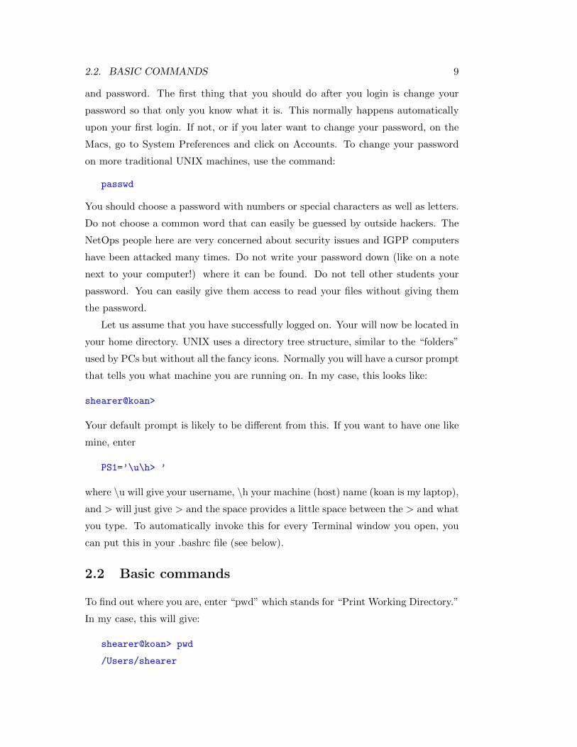
Let us assume that you have successfully logged on. Your will now be located in
your home directory. UNIX uses a directory tree structure, similar to the “folders”
used by PCs but without all the fancy icons. Normally you will have a cursor prompt
that tells you what machine you are running on. In my case, this looks like:
shearer@koan>
Your default prompt is likely to be different from this. If you want to have one like
mine, enter
PS1=’\u\h> ’
where \u will give your username, \h your machine (host) name (koan is my laptop),
and > will just give > and the space provides a little space between the > and what
you type. To automatically invoke this for every Terminal window you open, you
can put this in your .bashrc file (see below).
2.2 Basic commands
To find out where you are, enter “pwd” which stands for “Print Working Directory.”
In my case, this will give:
shearer@koan> pwd
/Users/shearer

10 CHAPTER 2. UNIX INTRODUCTION
This shows that I am located in my home directory (named shearer) in the Users
directory on my laptop.
You can list the contents of your current directory with the “ls” command:
shearer@koan> ls
(I’m not showing you the output because it’s too messy in my case!)
UNIX has an online set of manuals that may be accessed with the “man” com-
mand. For example, suppose you forgot what “ls” does. You could type “man ls”
and you would get a description of the ls command and its many options. One
annoying aspect of standard UNIX is that the man command output uses a form
of the VI editor rather than the normal window output, which permits scrolling up
and down in the window. When you enter “man ls” you will get a page of output on
the screen with a colon (:) at the bottom. If you enter the space bar, you will then
get the next page of output, etc. But you can’t scroll backwards using the window
scroll arrows. To go backwards, enter “b” at the colon prompt. When you get to
the final page, you will see END at the bottom. To leave the man pages and return
to the normal terminal, hit the ‘q’ key (for quit) at any point.
If you find this too annoying to deal with, you can always save the man pages
to another file. To do this, enter:
man ls > man.ls
The output will now be directed into a file named “man.ls” rather than to the screen.
To look at man.ls, use the ‘cat’ command:
cat man.ls
The ‘cat’ command prints a text file to the screen. The advantage in this case is that
you can use the scroll bar. Note that if you try to look at man.ls using a text editor,
you will likely see all kinds of weird control characters that are used to format the
screen output.
Of course, you risk cluttering up your directory with lots of files named “man.whatever”
if you do this a lot. If you don’t want to worry about deleting them, one solution is
to use the name “junk” as a temporary place to store output. If you already have a
file named junk, it will just overwrite the old file. This way, you only ever have one
“scratch” file in your directory at one time.
2.2. BASIC COMMANDS 11
Another approach, if you have access to the web, is to simply Google ‘unix man
ls’ to bring up the man pages, nicely formatted!
There usually are options to UNIX commands that can make them more useful
for what you want. For example, “ls” simply lists the file names in your directory.
If you want to find out how big they are or when they were last modified, then use
“ls -l” where the “l” stands for the long output option. In your home directory, you
will have a very important file called “.bashrc” (see below). This file will not appear
if you just enter “ls”. To make it appear, enter “ls -a” where the “a” stands for the
“all file” option.
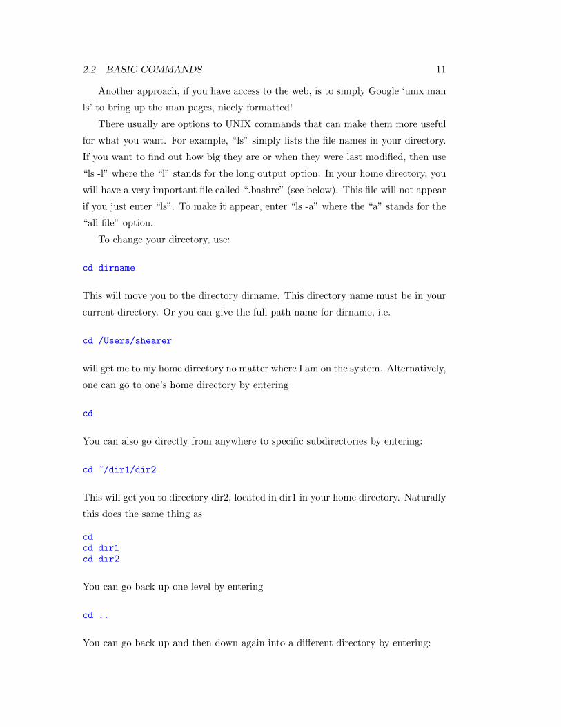
To change your directory, use:
cd dirname
This will move you to the directory dirname. This directory name must be in your
current directory. Or you can give the full path name for dirname, i.e.
cd /Users/shearer
will get me to my home directory no matter where I am on the system. Alternatively,
one can go to one’s home directory by entering
cd
You can also go directly from anywhere to specific subdirectories by entering:
cd ~/dir1/dir2
This will get you to directory dir2, located in dir1 in your home directory. Naturally
this does the same thing as
cdcd dir1cd dir2
You can go back up one level by entering
cd ..
You can go back up and then down again into a different directory by entering:

12 CHAPTER 2. UNIX INTRODUCTION
cd ../dir2
To create a new directory, use the “make directory” command:
mkdir dir1
It is often convenient to use a different naming convention for your directories in
order to distinguish them from your files. Some people put .dir after their directories.
For awhile I put d. in front of the directory names, which has the advantage of
grouping them together when “ls” is entered, since UNIX lists things in alphabetical
order. Most recently, I have been using all capital letters for the directory names.
This makes them more visible, but has the disadvantage of slowing down typing
their names (yes, UNIX is case sensitive!).
If you don’t want to use special names for directories or if you find yourself
in somebody else’s directory where they don’t do this, you can use the “ls -F”
command:
ls -F
This will add a / suffix to directory names and a * prefix to executable file names.
I like this so much that I have set this up as my default “ls” command by putting
an alias into my .bashrc file (more about this later).
2.3 Files and editing
Files can be simple ascii (text) files or they can be binary files, often the executable
versions of computer programs. One standard UNIX editor is called vi and is still
used by some of the old time programmers at IGPP who will insist that it is remains
the best editor. If you know all of its tricks it can be an extremely powerful editor.
You can do things, like cut and paste columns of numbers, that most editors can’t
do. It also has the advantage of running on any terminal so if you log in from home
you can still edit files.
If you know vi or decide that you want to learn it—more power to you. You will
not lose any points around here. However, vi is not mouse or window friendly and
is not favored by most students today. I have forgotten most of the vi that I once
knew (I used it to do my thesis back in the late Cretaceous).
Editors on the Mac include:

2.3. FILES AND EDITING 13
• TextEdit – You can find this in the applications folder. Be sure to set the
format (under Preferences) to Plain text and not Rich text, which will put in
control characters that will screw things up. You also will want to turn off
”smart quotes” and ”smart dashes” to avoid entering non-standard characters
not recognized by UNIX.
• nedit – This is supposed to run on all platforms and has more features than
textedit.
• emacs – this is a very powerful editor that is used by computing professionals.
It can do just about anything but may be somewhat harder to learn at first
than simpler editors.
• Xcode – special Mac editor designed for editing programming code
You can use any of these editors to create a new file or edit an existing file. Unix
file names are case sensitive. By convention, the type of file is often indicated by
.type, for example:
testprog.f for Fortran77 program source code
testprog.f90 for Fortran90 source code
testprog.c for C program source code
testprog.m for a MatLab script
testprog.o for an object file
figure1.ps for a Postscript file
figure1.gif for a GIF file
Be aware that the Mac Finder will hide many of these suffixes when you look at
file names within a Mac folder, but they will appear when you type “ls” in a Unix
Terminal window.
You may wish to create your own naming convention to keep track of your files.
When used with wildcards (see below) this will make it easy to list all files of a
particular type.
WARNING: Do not use a slash (/) or the dash character (-) in file names; this
may cause all kinds of problems for you. Use . or to separate the words. NEVER
USE BLANKS IN FILE OR DIRECTORY NAMES USED IN PROGRAMMING!!!
(I know this is common on Macs and PCs for document files but you will eventually
have big problems reading with your programs any file names with blanks)

14 CHAPTER 2. UNIX INTRODUCTION
2.4 Basic commands, continued
If you want to remove a file use the ‘rm’ command:
rm filename
If you want to change the name of a file, use the ‘mv’ (move) command:
mv filename1 filename2
If filename2 already exists, this will have the possibly undesired consequent of delet-
ing the original filename2. To guard against this, use the “-i” option:
mv -i filename1 filename2
Now if filename2 already exists, the computer will ask you first if you want to
overwrite this file.
mv can also be used to move files between directories:
mv filename dirname
will move filename into directory dirname (assuming dirname already exists!) where
it will have the same name. Note that this does the same thing as
mv filename dirname/filename
For convenience, you can leave off the /filename if the file is to keep the same
name. A note of caution: In this shortened version, if dirname does not exist as a
directory, then the name of filename will be changed to dirname.
The copy command works in a similar way:
cp filename1 filename2
makes a copy of filename1 called filename2.
cp -i filename1 filename2

2.4. BASIC COMMANDS, CONTINUED 15
will first ask if you really want to do this if filename2 already exists. You can copy
files to different directories in the same way as the mv command works.
Many people so prefer the -i option for mv and cp that they make it the default
option by defining an alias in their .bashrc file (see below) so that mv and cp become
“mv -i” and “cp -i”. I recommend that you do this—it is likely to save you some
grief in the future. If you are super cautious, you can also add the -i option for the
“rm” command, but I find this annoying because I normally intend to remove the
specified file when I use the “rm” command. Note that there is no “undo” command
in UNIX. Once a file is gone, it’s gone (unless you have a backup somewhere).
To remove a directory, use the “rmdir” command:
rmdir dirname
The directory must first be empty for this to work. To recursively remove a directory
and its contents use:
rm -r dirname
Use this with extreme caution to avoid accidentally deleting more than you intended!
2.4.1 Wildcards
UNIX commands become much more powerful when they are used with the wildcard
character * which can take on any ascii string1.
For example, suppose you wanted to list all files ending with .f the suffix used
to identify Fortran source code. Simply enter:
ls *.f
You could move all of these programs in a subdirectory called source.dir by
entering:
mv *.f source.dir
You might have a bunch of plot files called mypost1, mypost2, etc. You could
delete all of these at once by entering:
1The question mark (?) can also be used as a wildcard and in most cases will work the sameas *. However, * is preferred because it will avoid files with an initial . and thus you will notaccidentally delete your .bashrc file by entering something like “rm *rc”.

16 CHAPTER 2. UNIX INTRODUCTION
rm mypost*
For obvious reasons, be very careful when using * with the rm command. For
example, suppose you wanted to delete all files in your current directory that end
in %, which some text editors use to store the original version of edited files. To do
this, enter:
rm *%
Suppose, however, that you are careless when you type this and enter instead:
rm * %
This will delete everything in your current directory! So always look carefully at
what you have typed before hitting the return key when you are deleting files using
wildcards.
2.4.2 The .bashrc and .bash profile files
In your home directory, you can have files that are executed automatically under
certain conditions. These files begin with a ‘.’ and do not appear with the ‘ls’
command without the ‘-a’ option. They also do not appear in the Mac Finder, as
they are considered for advanced users only.
These files are useful for defining and customizing your environment. Typically
you will want them executed whenever you open a new Terminal window. Under
bash, this file is normally the .bashrc file. You may already have a default .bashrc
file set up by NetOps for your account, but you can modify this file to do what you
want.
For example, you can put aliases in your .bashrc file for the mv and cp commands
so that you don’t accidentally overwrite files:
alias cp=’cp -i’alias mv=’mv -i’
I also recommend that you make “ls -F” your default to make it easier to tell
the difference between directories and files:
alias ls=’ls -F’
If your want, you can also define a custom prompt:
2.4. BASIC COMMANDS, CONTINUED 17
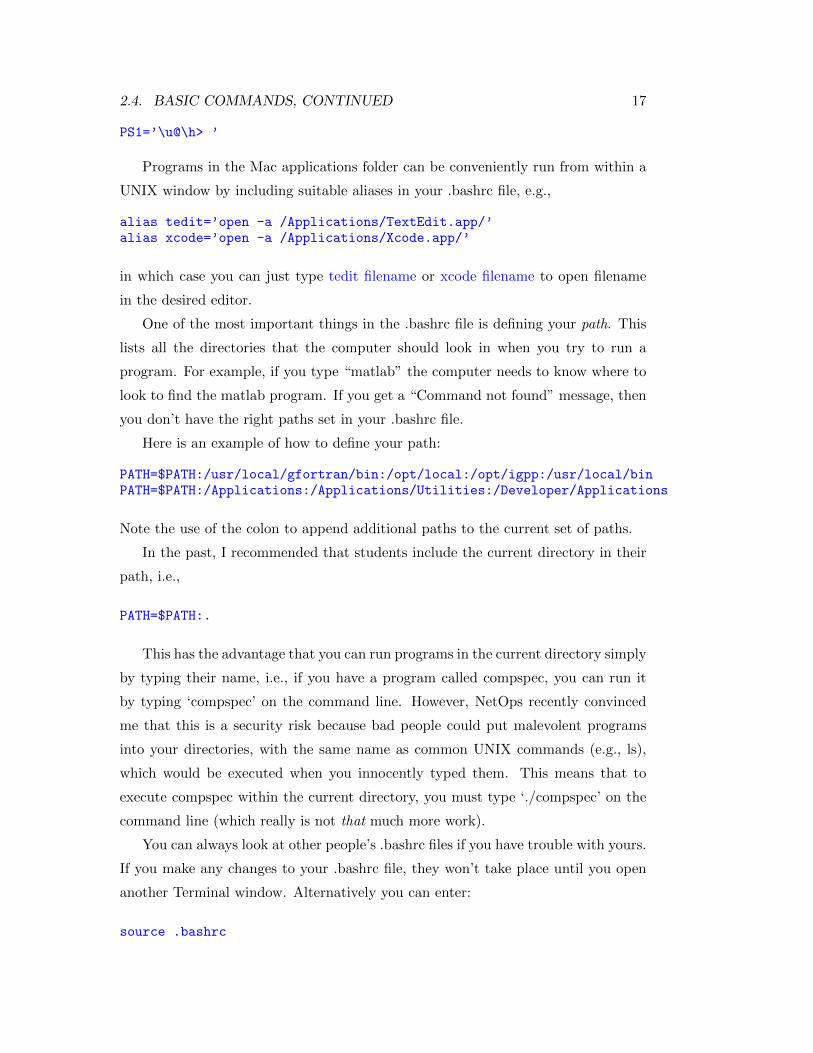
PS1=’\u@\h> ’
Programs in the Mac applications folder can be conveniently run from within a
UNIX window by including suitable aliases in your .bashrc file, e.g.,
alias tedit=’open -a /Applications/TextEdit.app/’alias xcode=’open -a /Applications/Xcode.app/’
in which case you can just type tedit filename or xcode filename to open filename
in the desired editor.
One of the most important things in the .bashrc file is defining your path. This
lists all the directories that the computer should look in when you try to run a
program. For example, if you type “matlab” the computer needs to know where to
look to find the matlab program. If you get a “Command not found” message, then
you don’t have the right paths set in your .bashrc file.
Here is an example of how to define your path:
PATH=$PATH:/usr/local/gfortran/bin:/opt/local:/opt/igpp:/usr/local/binPATH=$PATH:/Applications:/Applications/Utilities:/Developer/Applications
Note the use of the colon to append additional paths to the current set of paths.
In the past, I recommended that students include the current directory in their
path, i.e.,
PATH=$PATH:.
This has the advantage that you can run programs in the current directory simply
by typing their name, i.e., if you have a program called compspec, you can run it
by typing ‘compspec’ on the command line. However, NetOps recently convinced
me that this is a security risk because bad people could put malevolent programs
into your directories, with the same name as common UNIX commands (e.g., ls),
which would be executed when you innocently typed them. This means that to
execute compspec within the current directory, you must type ‘./compspec’ on the
command line (which really is not that much more work).
You can always look at other people’s .bashrc files if you have trouble with yours.
If you make any changes to your .bashrc file, they won’t take place until you open
another Terminal window. Alternatively you can enter:
source .bashrc

18 CHAPTER 2. UNIX INTRODUCTION
to make the changes immediately. But you will have to do this separately for each
window that you have open.
For reasons that I don’t completely understand, sometimes when you open a new
Terminal, your computer will execute a file called .bash profile instead of .bashrc.
Thus to make sure that your .bashrc file is always executed, you should have a
.bash profile file in your home directory that contains the following:
if [ -f ~/.bashrc ]; thensource ~/.bashrc
fi
which ensures that .bashrc is sourced, assuming it exists.
2.5 Scripts
One of the most powerful ways to use UNIX is to write scripts to run your programs.
This is an easy way to keep track of the input and output parameters and to make
changes without having to enter everything in again. For example, suppose you
have a program called mapfocal that asks you a bunch of questions like this:
shearer@koan> ./mapfocalreading cmt file...nev = 24584Enter output file nameglobalcmtmap.psEnter fill level, line thickness for conts0.93 1Enter line thickness for plate boundaries5Enter line thickness for beachballs1Enter minimum magnitude0Enter circle radius for beach balls (neg. for M0 scale)0.08(1) complete plot or (2) outline for test1Creating psplot postscript file : globalcmtmap.psnplot = 415shearer@koan 17>
After running this program, you decide that you would like to change the con-
tinent line thickness to 2. This is tedious if you have to type in everything again.
Instead you can write a script to run the program called ‘do.mapfocal’ that looks
like this:

2.5. SCRIPTS 19
./mapfocal << !globalcmtmap.ps0.93 1 !fill level, line thickness for continents5 !line thickness for plate boundaries1 !line thickness for beach balls0 !mininum magnitude0.08 !circle radius for beach balls (neg for mom scale, 0.08 looks nice)1 !1=complete plot or 2=outline for test!
This is just an ascii file that you write with your favorite text editor. The
comments following the numbered input (e.g., !min,max quake magnitude) are con-
venient if the program that you are running is robust enough to ignore additional
characters on lines that follow the numbers that are actually input into the program.
To run the script, simply enter:
./do.mapfocal
You may get a message which says:
do.mapfocal: Permission denied
This means that you don’t have execute permission on this file. To see what the
permissions are, use the ‘ls -l’ command:
shearer@koan> ls -l do.mapfocal-rw-r-xr-x 1 shearer 669 419 Oct 3 2012 do.mapfocal*
The ‘-rw-r–r–’ shows what the permissions are for the file. Columns 2-4 (rw-) are
your permissions as owner of the file. Columns 5-7 and 8-10 give the permissions for
your group and all others, respectively. The r means read permission, the w means
write permission and x means execute permission. In this case our problem is that
we have ‘rw-’ instead of ‘rwx’ To fix this, use the ‘chmod’ command:
chmod 755 do.mapfocal
This will give you rwx permission of file do.mapquake and will give everyone
else rx permission but not w permission. This is probably the most common set of
permissions you will want to set, assuming you are OK with others looking at your
code and running your programs, as long as they are not allowed to make changes.
Because the default permission for files created by most text editors does not give

20 CHAPTER 2. UNIX INTRODUCTION
execute permission for newly created scripts, I commonly have to use chmod before
I can run the scripts. To save time, I have created an alias in my .bashrc file called
fix:
alias fix=’chmod 755’
so that I can just enter ‘fix filename’ to correct the permissions for filename.
If you don’t want anyone else to be able to see your file, set
chmod 700 do.mapfocal
The three digits following chmod define the permissions for you, your group, and
everyone else respectively. As shown by the above examples, the most common to
assign are:
7 = read, write, and execute permission
5 = read and execute permission, but no write permission
0 = no permission
For more details see the chmod manual. You can also check and/or change per-
missions within the Mac Finder environment by clicking on a file or directory name
and then entering Command-i for information. This will show the sharing and
permission status.
The do.mapfocal script will run the mapfocal program and enter all of the re-
quired inputs. Notice that in this case I have added helpful comments to the numer-
ical input lines. You can do this with most programs and it will not affect the input
(at least for FORTRAN, I’m not so sure about C). You usually cannot, however, add
comments to the character inputs (e.g., globalcmtmap.ps in this example) because
it will consider them part of the name.
Now it’s easy to keep track of the inputs and to make changes without having
to re-enter everything. You can also put scripts together to run the program many
times:
./mapfocal << !globalcmtmap1.ps0.93 1 !fill level, line thickness for continents5 !line thickness for plate boundaries1 !line thickness for beach balls0 !mininum magnitude0.08 !circle radius for beach balls (neg for mom scale, 0.08 looks nice)1 !1=complete plot or 2=outline for test

2.6. FILE TRANSFER AND COMPRESSION 21
!
./mapfocal << !globalcmtmap2.ps0.93 2 !fill level, line thickness for continents5 !line thickness for plate boundaries1 !line thickness for beach balls0 !mininum magnitude1.1 !circle radius for beach balls (neg for mom scale, 0.08 looks nice)1 !1=complete plot or 2=outline for test!
In this case, you can make two different plots from the same script.
2.6 File transfer and compression
You often will want to get files from another computer. There are various ways to
do this. Today often files can simply be accessed via the web through a web browser,
or by directly mounting the disk of the other computer. An old fashioned method
of file transfer is the ftp (file transfer protocol) command, which is still used quite
a bit.
2.6.1 FTP command
One classic method of UNIX file transfer is the ftp command. For many public sites
and data centers this is done with anonymous ftp. You simply enter:
ftp othercomputer
where ‘othercomputer’ is the name (or IP address) of the other computer. When
you are asked to login, just enter ‘anonymous’ and then your e-mail address as a
password. Of course, if you have login permission on the other computer then you
can ftp to the machine even if it is not set up for anonymous ftp.
Once within ftp, you will get a ftp prompt. You then can use the ‘cd’ command
to get to the directory that you want and ‘ls’ to see the file names on the remote
computer. Finally use ‘get’ to bring the desired file to your own computer and
then ‘quit’ to exit ftp. If you want to get all of the files in the directory, use the
command ‘mget *’ and you will be prompted for each file name. If you don’t want
to be prompted, you can turn off the interactive mode by entering
ftp -i othercomputer

22 CHAPTER 2. UNIX INTRODUCTION
when you first invoke ftp. If you are getting binary files (rather than simple text
files), you should enter
type binary
at the FTP prompt before getting the files. Because ‘type binary’ will work with all
types of files, including ascii, it is a good practice to always enter ‘type binary’ as
soon as you enter ftp. The default for the Suns is ‘type ascii’ which does not work
with binary files.
If the remote computer objects to regular ftp for security reasons, you might try
‘sftp’ which is the secure ftp command.
If you have just a few files to transfer, you may want to use the secure copy
command:
scp filename *.ps [email protected]:./TRANSFER
will copy filename and all files ending with .ps from the current directory to the
TRANSFER directory in shearer’s account on rock.ucsd.edu (after first prompting
for the password). If you want to copy a directory, you need to use the -r (recursive)
option, i.e.,
scp -r dirname [email protected]:./TRANSFER
Note that one can also copy files from the remote computer to the current di-
rectory, i.e.
scp -r [email protected]:/net/moray2/scratch/dirname dirname_local
In this case the remote directory was on the /net/moray2 disk; notice how we
specified the complete path name.
2.6.2 File compression
Often the files that you retrieve will be compressed. Files can be compressed using
the UNIX ‘compress’ command:
compress filename

2.6. FILE TRANSFER AND COMPRESSION 23
This will change the name to filename.Z which tells you that it is compressed.
This is useful to save disk space when you will not be using the file for awhile. To
get back to the original file, use uncompress:
uncompress filename
You can compress a whole bunch of files by using wildcards:
compress *.ps
will compress all of your Postscript files, assuming you use the .ps suffix convention
for these files. These can be uncompressed with ‘uncompress *.ps’ as you would
expect.
An alternative compression method (not standard UNIX but usually available)
is invoked with the gzip command:
gzip filename
This changes the name to filename.gz with the reverse operation:
gunzip filename
The gunzip command will also decompress .Z files (but the uncompress command
will not decompress .gz files).
Note: On Macs, most compressed file formats can be uncompressed by simply
double-clicking on them.
You may find it useful to use compression yourself by compressing files that you
do not use very often in order to save space. I often do this when I want to get
some disk space but am too nervous to delete the files and too lazy to write them
to long-term backup.
2.6.3 Using the tar command
Often you may want to save or retrieve an entire directory of files. This is most
easily done using the ‘tar’ command. If you are within the directory containing the
files that you wish to save, then enter:
tar -cvf ../archive.tar .

24 CHAPTER 2. UNIX INTRODUCTION
The arguments are as follows:
-c create tar archive-v verify by printing file names to screen-f output file name will follow../archive.tar name for tar file (../ to put in next level up). tar every file in current directory
Alternatively you can save the entire directory and its contents from the level
above the directory:
tar -cvf programs.tar programs.dir
The tar file can then be FTPed to another machine. For even more efficiency
you may wish to compress the tar file first. The files can be retrieved as follows:
tar -xvf archive.tar
which will put all of the files in the archive into the current directory.
The tar command was originally written largely to write and retrieve backups,
etc., onto tape, in which case the file name (e.g, ../archive, programs.tar, etc.) in
the above examples is replaced with the name for the tape device. Today hardly
anyone uses tape drives because large capacity hard drives have gotten so cheap.
The Exabyte and DAT tape drives we used to have in the IGPP Barnyard have been
retired. If your advisor hands you an old data tape, you might check with NetOps
to see if they can read it, as they still have a few old tape readers.
2.6.4 Remote logins and job control
Often you will want to run on a different machine than the one that you are sitting
at. The other machine may be faster, have more memory, be connected to a large
hard drive with data, etc. To do this enter:
ssh machinename
and you can login and run remotely on this machine. Of course this will slow the
machine down for anyone else using it, so exercise some courtesy in doing this. One
option is to start your job with the ‘nice’ command:
nice do.bigjob
2.6. FILE TRANSFER AND COMPRESSION 25
where do.bigjob is the script that runs your program. The “nice” command lowers
the priority of your job so that it will not interfere with others using the machine.
You still may be unpopular, however, it you use a lot of memory on the machine.
Niceness levels range from 1 (highest) to 19 (lowest). The default for the nice
command is niceness 4 or 10 (depending upon which UNIX shell you are running).
To set the niceness to a specific value, you can specify a number, e.g.,
nice +15 do.bigjob
will run do.bigjob at niceness 15.
As a word of caution, most people don’t like to have other people run jobs on
their ‘personal’ machines (the ones in their offices) without permission, even if the
jobs are set to run at large niceness values.
To find out what jobs are running on your machine, you can use the ‘top’ com-
mand to list the most active jobs:
top
This will take over your window and update the results continuously until you
enter q for quit. The Process ID (PID) is listed, together with the username, the
niceness, the fraction of the CPU being used and other useful information. top is
interactive and you can input various commands (? for help, u to see only one user,
etc.). You can stop (kill) jobs from within the top program, or at the command line
using the “kill” command (see below).
If you did not originally use nice when you started a job you can ‘renice’ the job
from within top by entering ‘r’ Alternatively, if you know the job number you can
change the niceness at the command level, e.g.,
rock> renice +15 1132
where 1132 is the PID number (get from top program). You can renice more than
once, but only to raise the niceness level— you can never lower the niceless level
once it is set.
On the Macs, the “Activity Monitor” program (in Applications/Utilities) pro-
vides a convenient alternative to the UNIX top command.

26 CHAPTER 2. UNIX INTRODUCTION
2.7 Miscellaneous commands
Unix keeps track of your previous commands. To see them, enter
history
for history and it will list your last 30 commands. To repeat a past command, enter
! followed by line number in the ‘h’ list or simply the first few letters of the
command. To repeat the very last command, enter !!
Want to see what just the beginning or end of a big file looks like? Use the head
or tail command:
head filename ---lists the first 10 lines of the file
tail filename ---lists the last 10 lines of the file
To see a file one page at a time, use the ‘more’ command:
more filename
and then hit the space bar to advance one page at a time.
Want to see how many lines and words are in a text file? Use the word count
(‘wc’) command:
wc filename
This will list the number of lines, words, and bytes in the file. Often I just want to
know the number of lines, in which case it will run faster to use the -l option for
line:
wc -l filename
Lose track of where a file is? You can use the ‘find’ command:
find . -name filename -print
This will look in the current directory (that’s what the . is for) and below for
the file named ‘filename’ and then print where it is. What if you only know some
of the characters of the file? You can use a wildcard:
find . -name ’map*’ -print
2.7. MISCELLANEOUS COMMANDS 27
This will find all files that begin with ‘map’ and print them on your screen. Note
that you MUST enclose ’map*’ in apostrophes for this to work. Of course, most
computers now have built in search programs (e.g., Mac Spotlight) to locate files,
which may be more useful in many cases.
Unix has many powerful utility programs. One of these is the ‘sort’ command
to sort files in alphabetical or numerical order. Example:
sort +4 -n -b -r file1 -o file2
This sorts file1 and outputs the results to file2. The following options are used
in this example:
+4 skip first 4 fields (leave out to use beginning of line)-n numerical order (default is alphabetical order)-b ignore leading blanks-r reverse order (leave out for standard order)
NOTE: The +4 option no longer seems to work in Mac UNIX. Instead you set
the field number (normally the column number) using the -k option, i.e.
sort -k 5 -n -b -r file1 -o file2
should do the same thing as +4, i.e., skip 4 columns and sort on the 5th column.
To find out how much disk space is available use df (disk free):
df
This will not list all the disks on the system unless they have been mounted. Just
go to the disk that you are interested in and retry ‘df’ if it does not appear the first
time.
To see how much space you are using, the best command is
du -ks *
This will list the disk usage of each of your subdirectories. It is a good idea to
go through your directories once a month or so to delete unnecessary files and/or
compress large files that you don’t use very often.
To check for misspelled words in a file, use:
spell filename

28 CHAPTER 2. UNIX INTRODUCTION
This will list all words not found in a dictionary (which one?). Use the -b
option for the British spelling if you are submitting a paper to Nature. (NOTE:
unfortunately spell does not seem to work in Mac UNIX)
To reformat a text file to a uniform maximum line length of 72 characters, use:
fmt file1 > file2
This assumes that blank lines separate paragraphs. Line feeds within a paragraph
are removed and added as necessary to make the lines of approximately equal length.
This command is a useful feature if you use regular unix mail and create your
outgoing messages with a text editor. It is helpful when you want to change a line
in the middle of a paragraph because you don’t have to redo all the following lines
in order to make things look nice.
To preview a postscript file on the screen use:
gv filename.ps
which is an abbreviation for the old ghostview program.
2.7.1 Common sense
This should go without saying, but you never know. Do not download pornography,
hate literature, etc., on UCSD computers. You may get into BIG trouble (worse,
you could get your advisor into trouble!). You also should not illegally download
copyrighted material (musics, movies, etc.).
You should not consider UCSD e-mail to be completely private. Even deleted
e-mail is usually still on the computer system somewhere, often on daily and weekly
backup tapes. Be very careful when you reply to messages sent to a group of people
that you do not send your message to everyone on the list (unless that is your
intention).
Attempts at sarcasm and irony usually misfire in e-mails. It’s best to err on the
side of professionalism in your communications with your colleagues.
2.8 Advanced UNIX
This writeup so far contains most of what I have ever done with UNIX. You can go
pretty far with only 20 commands or so. However there are much more powerful
2.8. ADVANCED UNIX 29
things you can do. If you really want to be a UNIX guru, try reading up on pipes,
grep, awk, sed, etc. Then you will be able to write custom scripts to do all kinds of
neat things. Here are some examples:
grep dziewonski filename
This will print every line from file filename that contains the string Dziewonski.
grep -v dziewonski filename
This will print every line from file filename that does NOT contain the string
Dziewonski.
grep dziewonski filename > dz.lines
This works as above except the lines containing dziewonski are written to the file
dz.lines rather than printed to the screen.
grep dziewonski *
This lists lines containing dziewonski from ALL files within your current directory.
However, you may really want just the file names of the files that contain the string
dziewonski, in which case the following command will work better:
grep -l dziewonski *
This lists the file names of the files that contain the string dziewonski
grep ezxplot $(find . -name Makefile -print)
This is one that recently saved me when I could not find a program that I knew
I had written, but I did not know its name or which directory it was in. I knew,
however, that the program was compiled with a Makefile that would contain ezxplot
because this is necessary to make the program work. The grep command searches
for ezxplot in a list of file names returned by the find command. Note that the find
command must be enclosed with $(....).
ps -eaf
This lists all processes that are running on your machine

30 CHAPTER 2. UNIX INTRODUCTION
ps -eaf | grep shearer
This lists all of the processes that contain the string shearer in the output lines
of ps. In this case, the vertical line is a ‘pipe’ that directs the output of the first
command, ps, into the input of the second command, grep.
ps -eaf | grep shearer > junk
As above, but writes the output into file junk rather than to the screen.
kill PID
This kills a job with process ID number PID (obtained from the tops or ps com-
mand). This is useful for runaway jobs. For stubborn jobs, use the -9 option:
kill -9 PID
You can compare two files using the diff command:
diff file1 file2
This lists all differences between file1 and file2. This is useful if you have made some
changes to a file but cannot remember exactly what they are.
2.8.1 Some sed and awk examples
cat file1 | sed -n ’1,1p’ > file2Copy first line only of file1 to file2. Note that -nindicates that a line number range will follow, the pis to print the lines.
cat file1 | sed -n ’5,10p’ > file2Copy lines five to ten of file1 to file2.
cat file1 | sed -n ’2,$p’ > file2Copy all but the first line of file1 to file2. Note that$ indicates the last line.
cat file1 | sed ’s/Peter/Paul/’ > file2Copy file1 to file2, substituting "Paul" for the first "Peter"on each line.
cat file1 | sed ’s/Peter/Paul/g’ > file2Copy file1 to file2, substituting "Paul" for the every "Peter"on each line (note the "g" flag for global substitution).

2.9. EXAMPLE OF UNIX SCRIPT TO PROCESS DATA 31
cat file1 | sed ’s/^/Paul says /’ > file2Insert the prefix "Paul says " at the beginning of each line.Note that "^" means start of line
cat file1 | awk ’{print $5,$3,$1}’ > file2Assuming file1 has 5 columns of figures, this copies columns5, 3, and 1 to file2, in that order, omitting the 2nd and4th columns.
cat file1 | awk ’{print $2, $1*(-10)}’ > file2Switch columns 1 and 2 and multiply original 1st columnnumbers by -10.
cat file1 | awk ’{print substr($0,1,10) substr($0,31,10) substr($0,21,10)substr($0,11,10) substr($0,41,length($0)-40)}’ > file2
This copies file1 to file2, swapping the contents of columns 11-20and columns 31-40. $0 is the line, substr takes a chunk of it, thelast part prints the remainder of the line.
cat file1 | awk ’{print "Columns 11 to 20 are " substr($0,11,20)}’ > file2Start the beginning of each line with "Columns 11 to 20 are " and thenlist the contents of those columns in the input file.
Variations on the last few examples can be used to reformat ascii data files,
including those that do not have spaces between fields.
To learn more about sed and awk, please see Duncan Agnew’s notes on the class
website.
2.9 Example of UNIX script to process data
By combining UNIX commands into a script, it is possible to create very powerful
tools for processing data. Consider a simple example where we have a number of
data files contained in a data directory:
rock> cd data.dirrock> lsdata1 data2 data3
We have written a program to process the data in these files and write new data
files which we might want to call data1.proc, etc. The program is called procdata
and prompts the user for an input file name and an output file name, and, in this
simple example, a multiplier factor to scale the data. If the program is one level up
from the data directory, then:

32 CHAPTER 2. UNIX INTRODUCTION
rock> ../procdataEnter input file namedata1Enter output file namedata1.procEnter multiplier factor3rock>
To process all of the files in the directory, we could run the program for each
file, manually entering the file names. However, clearly this would get very tedious
if we had lots of files to process. We could modify the program to accept a list of
file names, but perhaps it is a complicated program that someone else wrote that
we don’t want to mess with. Another approach is to write a UNIX script to run the
program for all of the files in the directory. Here is one way to do this, using the
command file do.proc, which looks like this:
#!/bin/bash
\rm data.dir/*.proc
ls data.dir > filelistcd data.dir
# loop over data file namesfor filename in $(cat ../filelist)do
echo "processing file:" $filename
../procdata << !$filename$filename.proc200!
done
cd ..\rm filelist
Note that we start with
#!/bin/bash
to make sure we are in the bash environment. In general, scripts written for tcsh
will not work under bash, and vice versa.

2.9. EXAMPLE OF UNIX SCRIPT TO PROCESS DATA 33
This script is designed to be located in the same directory as the program, one
level up from the data directory. Note that within the script, we use ‘backslash rm’
instead of ‘rm’ so that any aliases that might require interactive verification of the
deletions are not performed. Otherwise the computer might prompt us to see if we
really want to delete the files and the script would not be prepared to handle this.
Next, we remove any existing processed files in the data.dir directory, using a
wildcard and assuming that the file names end in .proc
Next, we write a list of the data file names within data.dir into the file filelist.
Then we go into data.dir where we loop over the filenames contained in filelist,
using the lines
for filename in $(cat ../filelist)do
which assigns the variable filename sequentially to each line in filelist, each time
executing the lines in the script between ’do’ and ’done’ which terminates the loop.
$(....) is bash for “execute the UNIX command inside the parentheses.” In a simple
case in which the file names are always data1, data2, and data3, this line could have
been written as
for filename in data1 data2 data3
but this is not a very versatile way to write the script.
Note that comment lines start with #, i.e.,
# loop over data file names
is just to make the script easier to understand.
We use the echo command to output to the screen each file name that is being
processed. Note that we must include $ in front of the variable filename when it is
referred to after its definition.
We then run the procdata program (one level up, so we need the ../). The
procdata program is terminated within the script with the ! symbol.
Following the ‘done’ statement that completes the loop over the files, we go back
to the directory containing the program and delete filelist, as it is no longer needed.
The power of this script is that it can be run on a directory containing thousands
of files, just as easily as for a smaller number of files.

34 CHAPTER 2. UNIX INTRODUCTION
Now let’s explore some possible changes to this script. Perhaps we don’t want
all the program i/o lines to print on our screen. To write these to an external file,
we could write the following:
#!/bin/bash
\rm procdata.log\rm data.dir/*.proc
ls data.dir > filelistcd data.dir
# loop over data file namesfor filename in $(cat ../filelist)do
echo "processing file:" $filename
../procdata >> ../procdata.log << !$filename$filename.proc200!
done
cd ..\rm filelist
Now, the screen output from the program (all of the ‘Enter input file name’, etc.,
lines) are directed to a file called procdata.log, so the first thing we do is remove
any old versions of this file, if it exists.
In this example, we really did not need to generate the file filelist because we
eventually deleted it. Thus, we could have written the script as:
#!/bin/bash
\rm procdata.log\rm data.dir/*.proc
cd data.dir
# loop over data file namesfor filename in $(ls)do
echo "processing file:" $filename

2.10. COMMON UNIX COMMAND SUMMARY 35
../procdata >> ../procdata.log << !$filename$filename.proc200!
done
cd ..
We won’t have time in this class to go into the details of all of the different
things one can do in scripts like this. There are lots of books and websites on UNIX
that one can consult for this purpose, but most of us just pick up stuff as we need
it. The main point that I want to get across is that if you are spending lots of time
running programs manually, then you are wasting your time. Spend some of that
time learning how to write a UNIX script and you will be far better off in the long
run. Your work will be better documented and it will be much easier for you (and
others) to reproduce your work.
For example, geophysics students often write elaborate scripts to request data
from a data center, convert it to a more desirable format, perform quality control,
and then execute a series of processing steps that may involve a mixture of different
programs.
2.10 Common UNIX command summary
cat filename print filename on your screen
cd dirname change directory to dirnamecd .. go back up one levelcd go to home directorycd ~/dirname go to directory dirname in home directorycd ~otheruser go to home directory of otheruser
cp file1 file2 copy file1 to file2cp -i f1 f2 copy f1 to f2 but ask before overwriting f2
df list disk space on the different disksdu -ks * list disk usage for files/dirs in current directory
lpr -P silo filename send filename to printer silo
ls list files in directoryls -l listls -a list all files including those starting with .

36 CHAPTER 2. UNIX INTRODUCTION
ls -F flag directories by adding slash to their namels *.f list all files with ending with ".f"
mkdir dirname make directory dirname
mv file1 file2 change name of file1 to file2mv -i f1 f2 change name of f1 to f2 but ask before overwriting existing f2mv *.f src move all files ending in ’.f’ into existing directory src
pwd print working directory
rm filename remove filenamermdir dirname remove directory dirname (directory must be empty)
wc filename count words in filewc -l filename count lines in file

Chapter 3
A GMT Tutorial
Generic Mapping Tools, almost always called simply GMT, is a set of UNIX tools
for making map and plots written by Paul Wessel and Walter Smith. This software
is in the public domain and is still maintained by Wessel and Smith.
If you have an IGPP laptop, GMT should already be installed. If you need to in-
stall it on your own Mac, I recommend that you follow the NetOps Macports instruc-
tions at: https://igppwiki.ucsd.edu/wiki/pages/A0i460e/Installing Macports.html
To learn about GMT, there is a website at http://gmt.soest.hawaii.edu/ that
contains links to documentation, a GMT tutorial, and a number of examples. Often
the best strategy for figuring things out is to look through the examples and find
something close to what you want and use that as a starting point. If you Google
“GMT tutorial” you will find a number of useful sites.
Once you have learned a little bit about how to use GMT, it’s helpful to use the
online help documents as your primary reference. You can access these at the UNIX
command level by simply entering: man gmt pscoast or even just gmt pscoast,
although the latter option does not produce text as nicely formatted as the former.
But be warned, GMT is not very “user friendly”. If you are unfamiliar with some of
the features of the UNIX environment like piping output, etc., you may find it fairly
intimidating at first. However, it is extremely powerful in the number of things that
it can do and the time spent learning how it works will not be wasted as you will
become familiar with many useful UNIX tools. GMT is capable of producing very
nice maps and plots and is pretty much the industry standard for Earth Science
map making.
We begin with an example using the tool pscoast. You will ALWAYS want to
run GMT as a UNIX script (see Chapter 2). Here is one called do.gmt1:
37

38 CHAPTER 3. A GMT TUTORIAL
#!/bin/csh
gmt pscoast -R0/360/-90/90 -JQ180/6i -B60g30 -P -Dc -G150 >! map.ps
gv map.ps
The first line, #!/bin/csh, invokes the C-shell environment. The script will run
without this, but it is probably safest to always go into the C-shell because most
example GMT scripts do this. Presumably in some cases it may make a difference.
Next we encounter gmt pscoast which invokes the GMT program that draws
coastlines. Note that older versions of GMT than GMT5 will leave out the “gmt”
and start the command with “pscoast” alone. Older GMT scripts will not work
under GMT5 unless you modify them by adding “gmt” in front of all the commands
(there are other changes as well, but this is the biggest one).
GMT programs have a lot of options that, in UNIX style, are invoked with a
dash and a letter on the same line (e.g. -P, -Dc, etc.). The output of the program
is directed to the Postscript file map.ps. Note that we use >! instead of > to avoid
getting an error message if map.ps already exists; but beware, you will overwrite
any existing map.ps file.
To get a full list of options, simply type man gmt pscoast. But for now, let us
examine the arguments in our example:
-R0/360/-90/90
This sets the map limits of longitude (lon1=0, lon2=360), and latitude (lat1 =
−90, lat2 = 90). Note that we could have written this with a space between the
“R” and the zero (”0”) immediately following. Most people leave this space out to
more easily separate the different commands.
-JQ180/6i
This specifies the map projection to be cylindrical equidistant (a simple linear
scaling of lat/lon). The center meridian is set to 180 degrees; the plot width is set
to 6 inches (the “i” means inches). A very large number of different map projections
are available!
-B60g30
39
This sets the labeled lat/lon lines to 60 degree intervals and the unlabeled lines
to 30 degree intervals
-P
Specifies “portrait” mode so that the plot is not rotated by 90 degrees as in
“landscape” mode (default).
-Dc
Sets the resolution of the coastline to “c” for crude. This is all that is required
for a small map of the whole globe. For larger maps or closeups, higher resolution
will be required. The available options are: (f)ull, (h)igh, (i)ntermediate, (l)ow and
(c)rude. Note that the full resolution files require over 55Mb of data and provide
great detail, which would be wasted in this case. For efficiency in generating and
storing the plots, you should only use as much resolution as you need and thus -Df
should be reserved for extreme closeups. The default is (l)ow resolution.
-G150
Specifies the grayshade level for the continent shading from 0 (black) to 255
(white). These nonintuitive units are a Postscript convention!
The GMT part of the script is entirely the “gmt pscoast” command and we
could stop there. Running the script would creates the map.ps file, which could
examine after the script is finished. However, it’s convenient to display the result
immediately, so we add a line to preview the Postscript file:
gv map.ps
After running the script do.gmt1, you should get a Postscript plot that looks
like this:

40 CHAPTER 3. A GMT TUTORIAL
If you open the file in gv, you will notice that there is a lot of white space
around the plot and it is not centered on the page. The white space is not a big
problem, as you can remove the space if you want by opening the .ps file in Preview
and then saving it as a .eps or pdf file. You can also import .ps files directly into
Adobe Illustrator for resizing, adding labels, etc. However, if you generate a plot
larger than the page size, GMT will truncate it. To give yourself more room, set the
media type to ArchE, which is poster size, using gmtset PAPER MEDIA ArchE.
The plot is not centered on the page because the default position for the lower
left corner is at x=1inch, y=1inch. We can change this by specifying the x and y
positions directly:
-X1.2i -Y4i
This sets the lower left corner to 1.2 inches from the left edge and 4 inches from
the bottom.
You may also decide that you don’t want grid lines drawn on the plot so we
remove the “g30” from the -B command:
-B60
This puts a label on the latitudes and longitudes every 60◦, but doesn’t draw the
grid.
You may prefer a smaller font. This can be set with GMTSET before calling
pscoast:

41
gmt gmtset FONT_ANNOT_PRIMARY 10
The resulting script (do.gmt2) is:
#!/bin/csh
gmt gmtset FONT_ANNOT_PRIMARY 10
gmt pscoast -R0/360/-90/90 -JQ180/6i -B60 -P -Dc -G150 \
-X1.2i -Y4i >! map.ps
gv map.ps
Note that we used a backslash to indicate that the line continues to the next
line. In this way we can avoid making our lines too long.
This script produces:
After running the do.gmt2 script, if we run the do.gmt1 script again, we will be
surprised to see that the font size is the same as we just got using the do.gmt2 script.
In other words, do.gmt1 is not working exactly the same as it did before. What is
going on? The answer is contained in a file called gmt.conf that GMT creates (or
updates) in your current directory. It contains all of your “custom” settings, like
font size, that you specify when running gmt. If you look at this file, you will see
that the font size is what you specified in do.gmt2. When you run GMT, it looks
to see if you have a gmt.conf file and will take parameter values from this file if it
exists. This is a way to customize GMT to your own preferences. These might vary
from project to project, in which case you can maintain different gmt.conf files in
different directories for each project. If you don’t want to read from a gmt.conf file

42 CHAPTER 3. A GMT TUTORIAL
when you run your script, just rename the gmt.conf file to something else before
running the script.
Next, suppose you have a file containing the coordinates of some seismic stations
which we wish to plot on this map. The file is called station.list and its first five
lines are:
9.02920 38.76560 2442 AAE
42.63900 74.49400 1645 AAK
37.93040 58.11890 678 ABKT
51.88370 -176.68440 116 ADK
-13.90930 -171.77730 706 AFI
Here is a script (do.gmt3) that will plot these points on our map:
#!/bin/csh
gmt gmtset FONT_ANNOT_PRIMARY 10
gmt pscoast -R0/360/-90/90 -JQ180/6i -B60 -P -Dc -G150 \
-X1.2i -Y4i -K >! map.ps
gmt psxy -O -R -JQ180/6i -St0.06i -G0 -: station.list >> map.ps
gv map.ps
The first part of the script is the same as before, except that the -K is necessary
to tell GMT to keep the Postscript file open (i.e., don’t put a “showpage” at the
end of the file) so that more can be added to the file.
Next, we use gmt psxy to read and plot the x-y points from file station.list. We
use >> to append the output onto the end of the map.ps file. Note that > or >!
would not work here because it would overwrite the file instead of adding to it.
WARNING: It appears that psxy sometimes will not work if the numbers start
in the first column of the input file. If you are having trouble getting psxy to work,
try adding a blank character to the start of each line.
The arguments of psxy are as follows:
-O
Indicates that this is an overlay onto an existing Postscript file to avoid the initial-
izations at the beginning of the file. VERY IMPORTANT: Every GMT command
but the first should have -O, every GMT command but the last should have -K.

43
-R
Sets the plot boundaries (defaults to those set by pscoast)
-JQ180/6i
Sets the map projection (according to the manual, just saying -JQ should automat-
ically match the previous projection (i.e., you don’t need the 180/6i) but I have not
always found this to be true. Try it and see what happens with your version of
GMT!).
-St0.06i
Plots xy points as (t)riangles of 0.06 inch width. Other options are (c)ircle, (d)iamond,
(s)quare, (i)nverted triangle, (x)cross, and (v)ector. In the case of the vector, the
direction and length are also read from the file (see manual).
-G0
Set fill parameter to 0 (black). This will fill in the triangles.
-:
This tells the program that the data are to be read as y-x pairs. The default is x-y, or
(lon, lat) in our case. For seismology this option is very useful because coordinates
are usually given as lat, lon rather than the other way around.
Note that the program automatically converts the longitude convention of the data
points (-180 to 180) to the longitude convention of the map (0 to 360). This is a
nice feature of GMT.

44 CHAPTER 3. A GMT TUTORIAL
0˚
0˚
60˚
60˚
120˚
120˚
180˚
180˚
240˚
240˚
300˚
300˚
0˚
0˚
−60˚ −60˚
0˚ 0˚
60˚ 60˚
Now let’s try a different map projection, plot the points in red, and add a title
in a script called do.gmt4:
#!/bin/csh
gmt gmtset FONT_ANNOT_PRIMARY 10
gmt pscoast -R-180/180/-90/90 -JH0/6i -Bg0:."IRIS FARM stations": \
-P -Dc -G150 -X1.2i -Y4i -K >! map.ps
gmt psxy -O -R -JH -St0.06i -G255/0/0 -: station.list >> map.ps
gv map.ps
The changed commands are as follows:
-JH0/6i
Invokes the equal-area Hammer projection with 6 inch width
-Bg0:."IRIS FARM stations":
The 0 results in no grid lines or labels The title is set off with :.” and “: (weird!)
-G255/0/0
Define the fill for the xy plot as red=255, green=0, blue=0
The result is:
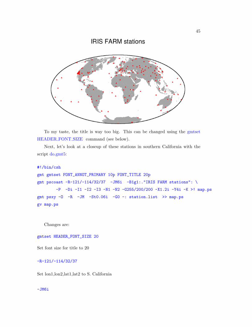
45
To my taste, the title is way too big. This can be changed using the gmtset
HEADER FONT SIZE command (see below).
Next, let’s look at a closeup of these stations in southern California with the
script do.gmt5:
#!/bin/csh
gmt gmtset FONT_ANNOT_PRIMARY 10p FONT_TITLE 20p
gmt pscoast -R-121/-114/32/37 -JM6i -B1g1:."IRIS FARM stations": \
-P -Di -I1 -I2 -I3 -N1 -N2 -G255/200/200 -X1.2i -Y4i -K >! map.ps
gmt psxy -O -R -JM -St0.06i -G0 -: station.list >> map.ps
gv map.ps
Changes are:
gmtset HEADER_FONT_SIZE 20
Set font size for title to 20
-R-121/-114/32/37
Set lon1,lon2,lat1,lat2 to S. California
-JM6i

46 CHAPTER 3. A GMT TUTORIAL
Use Mercator projection, width = 6 inches
-B1g1:."IRIS FARM stations":
Label and draw grid lines every 1 degree and use same title
-I1 -I2 -I3
Plot permanent major rivers, additional major rivers, and additional rivers, respec-
tively
-N1 -N2
Plot nation boundaries and state boundaries, respectively
-G255/200/200
Fill land areas with red=255, green=200, blue=200 — an unsightly shade of pink:
IRIS FARM stations
239˚
239˚
240˚
240˚
241˚
241˚
242˚
242˚
243˚
243˚
244˚
244˚
245˚
245˚
246˚
246˚
32˚ 32˚
33˚ 33˚
34˚ 34˚
35˚ 35˚
36˚ 36˚
37˚ 37˚

47
Next, let’s add lines that show the traces of mapped faults in southern California.
For this, we use a file called calif.flts that has the following format:
370.0000 99.0000-115.5496 32.9312-115.5419 32.9142-115.5358 32.9029-115.5276 32.8890370.0000 99.0000-115.9218 32.9916-115.9096 32.9849-115.8936 32.9745-115.8729 32.9655-115.8398 32.9498-115.8216 32.9410-115.7983 32.9295-115.7796 32.9228370.0000 99.0000-115.8391 33.0127-115.8205 33.0069-115.8017 33.0015-115.7892 32.9973etc.
The faults are defined as (lon, lat) pairs. The creator of this file used a value of
(370, 99) to separate the different faults because 370 is off the map (longitude only
goes to 360). However, as we will describe below, GMT allows us to explicitly define
any string we want to separate the line segments that GMT draws on the map.
To plot these faults on our map of the southern California stations, we can use
the psxy command a second time in the script do.gmt6:
#!/bin/csh
gmt gmtset FONT_ANNOT_PRIMARY 10p FONT_TITLE 20p
gmt gmtset IO_SEGMENT_MARKER ’370’
gmt pscoast -R-121/-114/32/37 -JM6i -B1:."IRIS FARM stations": \
-P -Di -I1 -I2 -I3 -N1 -N2 -G255/200/200 -X1.2i -Y4i -K >! map.ps
gmt psxy -O -R -JM -W1p,255/0/0 calif.flts -K >> map.ps
gmt psxy -O -R -JM -St0.15i -G0/0/255 -: station.list >> map.ps
gv map.ps
Changes are:
-B1:."IRIS FARM stations":

48 CHAPTER 3. A GMT TUTORIAL
We removed the g0 so we don’t plot grid lines which might get confused with the
faults.
We plot the faults using:
psxy -O -R -JM -W1p,255/0/0 calif.flts -K >> map.ps
In the fault file, lines that start with ‘370’ mark the segment boundaries, i.e.,
they separate the series of points that defines each individual fault. Without these
separators, the program would draw lines between the end of one fault and the
beginning of the next fault and the plot would look like a mess. In GMT, the
default separator is the character ‘>’ but we define our own separator using
gmt gmtset IO_SEGMENT_MARKER ’370’
In GMT4, this could have been done using:
psxy -O -R -JM -M’370’ calif.flts -K >> map.ps ****DON’T USE IN GMT5
but the ‘-M ’ option has been removed (deprecated) from psxy in GMT5 in favor of
IO SEGMENT MARKER.
WARNING: The quotes around 370 (or whatever string you want to use as a
separator) MUST be the apostrophe character and not any kind of “smart quotes”
that your text editor may want to use. If you are using the Mac TextEdit program,
go to Preferences and turn off the Smart Quotes.
We control the width and color of the fault lines using
-W1p,255/0/0
This draws the line with linewidth=1p (one point) and color red=255, green=0,
blue=0
Note that we do not need the -: option because the points are already given as
(lon, lat).
We plot the stations last so that they will go on top of the faults. We change
the symbol size and the color:
-St0.15i
plot triangles 0.15 inches high
-G0/0/255

49
plot with red=0, green=0, blue=255
Note that -K is needed on every command except the last; -O is needed on ev-
ery command except the first. (***THIS IS KEY TO GETTING GMT SCRIPTS
TO WORK PROPERLY!!! CHECK THIS FIRST WHEN YOU HAVE PROB-
LEMS.***)
The script do.gmt6 results in the plot:
(Are there really no faults in eastern southern California?)
We often will want to include labels on our plot. The following script do.gmt7
adds four labels to our map using the pstext command:
#!/bin/csh
gmt gmtset FONT_ANNOT_PRIMARY 10p FONT_TITLE 20p
gmt gmtset IO_SEGMENT_MARKER ’370’
gmt pscoast -R-121/-114/32/37 -JM6i -B1:."IRIS FARM stations": \
-P -Di -I1 -I2 -I3 -N1 -N2 -G255/200/200 -X1.2i -Y4i -K >! map.ps

50 CHAPTER 3. A GMT TUTORIAL
gmt psxy -O -R -JM -W1p,255/0/0 calif.flts -K >> map.ps
gmt psxy -O -R -JM -St0.15i -G0/0/255 -: station.list -K >> map.ps
echo "-120 32.5 18 0 2 BL Pacific" | gmt pstext -O -R -JM -K >> map.ps
echo "-116.5 32.2 18 0 2 BL Mexico" | gmt pstext -O -R -JM -K >> map.ps
echo "-116.5 36.2 15 -45 2 BL California" | gmt pstext -O -R -JM -K >> map.ps
echo "-116.5 36.55 15 -45 2 BL Nevada" | gmt pstext -O -R -JM >> map.ps
gv map.ps
The pstext command expects to read from a file containing a list of labels in
a certain format. However, in this case we avoid the need for a separate input file
with the labels by using the UNIX echo command to pipe the required inputs into
pstext one line at a time. For example,
echo "-120 32.5 18 0 2 BL Pacific" | pstext -O -R -JM -K >> map.ps
adds the label “Pacific” to the plot at the (lon, lat) position (-120, 32.5) using
font size 18, at an angle of 0 degrees (measured CCW from horizontal), using font
number 2 (try different numbers and see what you get!), and positioned so that the
reference lon/lat is at the BottomLeft of the label (L, C, R = left, center, right; T,
M, B = top, middle, bottom).
The resulting plot is:
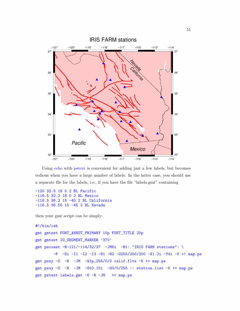
51
Using echo with pstext is convenient for adding just a few labels, but becomes
tedious when you have a large number of labels. In the latter case, you should use
a separate file for the labels, i.e., if you have the file “labels.gmt” containing
-120 32.5 18 0 2 BL Pacific-116.5 32.2 18 0 2 BL Mexico-116.5 36.2 15 -45 2 BL California-116.5 36.55 15 -45 2 BL Nevada
then your gmt script can be simply:
#!/bin/csh
gmt gmtset FONT_ANNOT_PRIMARY 10p FONT_TITLE 20p
gmt gmtset IO_SEGMENT_MARKER ’370’
gmt pscoast -R-121/-114/32/37 -JM6i -B1:."IRIS FARM stations": \
-P -Di -I1 -I2 -I3 -N1 -N2 -G255/200/200 -X1.2i -Y4i -K >! map.ps
gmt psxy -O -R -JM -W1p,255/0/0 calif.flts -K >> map.ps
gmt psxy -O -R -JM -St0.15i -G0/0/255 -: station.list -K >> map.ps
gmt pstext labels.gmt -O -R -JM >> map.ps

52 CHAPTER 3. A GMT TUTORIAL
gv map.ps
To my taste, the California and Nevada labels should be moved a bit down
the CA/NV border to the lower right. However, there are limits to how much “fine
tuning” of plots should be done using GMT because getting everything exactly right
for a publication quality plot can be tedious. Precise adjustment of labels and other
plots details can be done far more easily using interactive WYSIWYG programs like
Adobe Illustrator. Thus, despite what I said in the class introduction about how
you should use scripts to ensure the reproducibility of your results, I generally make
an exception when preparing plots for publication. The distinction is between what
you need to do to see the science results and what you do at the very end when you
are preparing plots for talks, papers, posters, etc. The important thing is to wait to
use Illustrator until you are certain that you have the final version of a plot. Before
that point, script-generated working versions of your plots should be adequate.
3.0.1 Setting default values
After you have used GMT for awhile, you may find that all your scripts have many
of the same lines, i.e., you always want to be in Portrait mode, or change the
header font size, etc. For convenience, GMT provides a way to customize your
GMT environment, i.e., to change the default parameter values. To do this, all you
have to do is edit your gmt.conf file, which should be in the same directory as your
scripts. If the file does not already exist, GMT automatically generates this file
when you first run GMT. It will have the standard default values, except for any
values that you explicitly change when you run GMT.
There are a large number of parameter choices in this file. As you gain experience
with GMT, you will likely want to set many of these to reflect your own preferences
for how things should look. Once they are in your gmt.conf file, then you don’t need
to set them each time in your GMT scripts.
Chapter 4
LaTeX
Someday you will want to publish the results of your research. IGPP scientists
typically use either Word or Latex for this purpose. Most of you probably already
know how to use Word. It is very easy to use (WYSIWYG) and is the “standard”
word processor of choice in many institutions. It is not, however, ideal for writing
scientific articles. It has particular difficulty handling equations and specialized
typesetting requirements. A far better choice is LaTeX. Guess what these notes are
written in!
Advantages of LaTeX:
1. It is in the public domain so you are not supporting the Evil Empire.
2. You can run it on Macs, PCs or UNIX machines.
3. By using macros, it is a far more powerful and versatile system than all the
pull down menu stuff you find in most commercial word processors.
4. AGU uses LaTeX for its electronic submission of articles and abstracts. They
provide macros to match the style of their journals so that preparing camera-
ready copy is trivial.
5. You can produce beautiful looking equations much more easily than with pro-
grams like Word.
LaTeX takes a little while to learn at first, but you will find it well worth your
effort. I will describe running LaTeX from the UNIX command line although I
am actually most familiar with using it on my Mac using a fancy implementation
(TexShop), which you can download from:
53

54 CHAPTER 4. LATEX
http://pages.uoregon.edu/koch/texshop/
4.1 A simple example
Use your favorite text editor to create the file samp1.tex (an example from the Latex
book, Kopka and Daly, A Guide to Latex2e):
\documentclass{article}\begin{document}Today (\today) the rate of exchange between the British poundand the American dollar is \pounds 1 = \$1.63, an increase of1\% over yesterday.\end{document}
which will produce:
Today (September 24, 2018) the rate of exchange between the British pound and
the American dollar is £1 = $1.63, an increase of 1% over yesterday.
The document must first define a document class. Options are book, report, arti-
cle, or letter. The guts of the document are then enclosed between the \begin{document}and \end{document} commands.
This example highlights some of the special characters and macros in Latex. The
following characters are normally interpreted as Latex commands:
$ & % # _ { }
To print these out in your text, you must precede them with a backslash, i.e.,
\$ \& \% \# \_ \{ \}
In this example, ‘\today’ invokes a macro to print today’s date and ‘\pound’
will print the British pound symbol. From this example you can see that Latex is
not WYSIWYG! To typeset this document, enter:
latex samp1
Assuming you have no errors in the input file, this will generate the file samp1.dvi.
To preview this file, enter:
xdvi samp1

4.2. EXAMPLE WITH EQUATIONS 55
To convert the file to a Postscript file, enter:
dvips samp1 -o samp1.ps
Notice that Latex automatically indented the first line of the paragraph. To
avoid this, use the command for the target paragraph:
\documentclass{article}\begin{document}\noindentToday (\today) the rate of exchange between the British poundand the American dollar is \pounds 1 = \$1.63, an increase of1\% over yesterday.\end{document}
To globally change the paragraph indenting, you can change the default for this
directly:
\documentclass{article}\begin{document}\setlength{\parindent}{0.5in}Today (\today) the rate of exchange between the British poundand the American dollar is \pounds 1 = \$1.63, an increase of1\% over yesterday.\end{document}
This will now indent all paragraphs by 0.5 inches. To remove paragraph indent-
ing, just set this parameter to zero. Latex ignores the carriage returns at the ends
of each line in the input file. It also ignores extra blanks; it only considers the first
blank. New paragraphs are defined by adding a blank line between blocks of text.
4.2 Example with equations
\documentclass{article}\begin{document}\setlength{\parindent}{0.0in}
The function $X(p)$ is more nicely behaved than $T(X)$ since it does notcross itself (there is a single value of $X$ for each value of $p$), butthe inverse function $p(x)$ is multi valued. An even nicer function isthe combination\begin{equation}

56 CHAPTER 4. LATEX
\tau(p) = T(p) - pX(p),\end{equation}where $\tau$ is called the {\it delay time}. It can be calculated verysimply:\begin{equation}\tau(p) = 2 \int_0^{z_p} \left[ {u^2 \over {(u^2-p^2)^{1/2}}} -{p^2 \over {(u^2-p^2)^{1/2}}} \right] \, dz
\end{equation}or\begin{eqnarray}\tau(p) &=& 2 \int_0^{z_p} (u^2-p^2)^{1/2} \, dz \\
&=& 2 \int_0^{z_p} \eta(z) \, dz\end{eqnarray}where $\eta$ is the vertical slowness.
\end{document}
which typesets as:
The function X(p) is more nicely behaved than T (X) since it does not cross itself(there is a single value of X for each value of p), but the inverse function p(x) ismulti valued. An even nicer function is the combination
τ(p) = T (p)− pX(p), (4.1)
where τ is called the delay time. It can be calculated very simply:
τ(p) = 2
∫ zp
0
[u2
(u2 − p2)1/2− p2
(u2 − p2)1/2
]dz (4.2)
or
τ(p) = 2
∫ zp
0(u2 − p2)1/2 dz (4.3)
= 2
∫ zp
0η(z) dz (4.4)
where η is the vertical slowness.
Note that equations within the text are enclosed with $ signs. \begin{equation}and \end{equation} are used to put the equation on a separate line. Variables
within the equations are automatically put into italics. Greek letters are defined
as \tau, \eta, etc. Equations are automatically numbered (this can be changed if
desired). Subscripts are defined with the underscore ( ), superscripts with the carat.
Fractions are written as, for example, {x \over y}. \int is for the integral symbol;
note how the limits are written. Curly brackets are used to separate things—they
do not appear in the typeset version.

4.3. CHANGING THE DEFAULT PARAMETERS 57
The \begin{eqnarray} section is used to align the = signs in the two lines of
equations. Note that &=& is used to define what it is that is being aligned. Every
line except the last line has a carriage return (\\). Although TeX generally does
an excellent job of spacing equations, sometimes some fine tuning will help. In this
case \, is used to place a tiny amount of space before the dz.
4.3 Changing the default parameters
4.3.1 Font size
There is a standard font size declared for each document class. In most cases this
is Roman 10 pt. One easy way to change the size is with the following commands,
arranged in increasing order of size:
\tiny\scriptsize\footnotesize\small\normalsize\large\Large\LARGE\huge\Huge
4.3.2 Font attributes
\itshape = switch to italics\slshape = switch to slanted font\upshape = switch to upright (normal) font
\bfseries = switch to bold\mdseries = switch (back) to regular weight
These commands can be invoked in several different ways to put “in situ” in italics
and then return to normal font:
\itshape in situ \upshape
OR
{\itshape in situ}

58 CHAPTER 4. LATEX
OR
\begin{itshape}in situ\end{itshape}
These different options also apply to the font sizes listed above. Here is an
example of how these options can be used:
\documentclass{article}\begin{document}
Let’s test different ways to say \itshape in situ \upshapein italics. There are several different ways to say{\itshape in situ} in italics; indeed\begin{itshape}in situ\end{itshape}can be written in italics in at least three different ways.
Next let’s experiment with {\large large}, {\Large Large},and {\LARGE LARGE} type, as well as {\small small},{\footnotesize footnotesize}, and {\scriptsize scriptsize}type.
\end{document}
which produces:
Let’s test different ways to say in situ in italics. There are several different waysto say in situ in italics; indeed in situ can be written in italics in at least threedifferent ways.
Next let’s experiment with large, Large, andLARGE type, as well as small,
footnotesize, and scriptsize type.
4.3.3 Line spacing
There is a default line spacing created whenever a new font is selected. Here are
examples of two different ways that this can be changed:
\setlength{\baselineskip}{10pt} Change line spacing to 10 point(single spacing for 10pt font).
\renewcommand{\baselinestretch}{2} Change normal (single) line spacingby a factor of 2. This will resultin double spacing. This must becalled before \begindocument or beforea new font declaration.

4.4. INCLUDING GRAPHICS 59
Here is an example:
\documentclass{article}\begin{document}\setlength{\baselineskip}{20pt}Today (\today) the rate of exchange between the British poundand the American dollar is \pounds 1 = \$1.63, an increase of1\% over yesterday. Let’s write one more line here so that weget up to three lines and can see the spacing better.\end{document}
which produces:
Today (September 24, 2018) the rate of exchange between the British pound and
the American dollar is £1 = $1.63, an increase of 1% over yesterday. Let’s write
one more line here so that we get up to three lines and can see the spacing better.
4.4 Including graphics
Postscript, EPS, and PDF files can easily be embedded as figures in a Latex docu-
ment by including Latex extension packages such as graphics or graphicx. Here is
an example that uses graphicx:
\documentclass{article}\usepackage{graphicx}\begin{document}\setlength{\baselineskip}{20pt}We are now going to show how to embed a Postscript file intoa LaTex document using the includegraphics command.
\begin{figure}[h]\begin{center}\includegraphics[scale=0.7]{figures/plot_1.pdf}\end{center}\caption{Here is the caption for this plot. This will be automaticallypositioned below the plot.}\end{figure}
And then here is some more text to show where the next block of textwill appear. Blah, blah, blah...\end{document}
which will produce:
We are now going to show how to embed a Postscript file into a LaTex document
using the includegraphics command.

60 CHAPTER 4. LATEX
Figure 4.1: Here is the caption for this plot. This will be automatically positionedbelow the plot.
And then here is some more text to show where the next block of text will
appear. Blah, blah, blah...
Note that the graphicx package is loaded with the \usepackage{graphicx} com-
mand at the start of the file. The \begin{figure} macro has various options for
where the figure will be positioned, including at the present location in the text [h],
or at the top [t] or bottom of the page [b]. These options can be combined, i.e., [tb]
will position the figure at either then top or bottom of the page. In this example,
the figure is scaled to 70% of its original size. Depending upon how the figure is
positioned in the PDF file, you also may need to apply a “bounding box” to remove
the surrounding white space using the bb= option, e.g.,
\includegraphics[bb=2in 4in 7in 9in, scale=0.7]{figues/plot_1.pdf}
which specifies exactly what part of the page will be windowed and displayed. This
is necessary for PDF figures that appear in only part of an entire page and it can be
tedious to find the right bounding box. In my experience, an easier option is to use
the Mac Preview program to open Postscript or EPS files (from Adobe Illustrator

4.5. WANT TO KNOW MORE? 61
or other graphics programs) and then save them within Preview as PDF files. In
this case, they are tightly windowed and the bb option is not needed.
Figures are automatically numbered; users have control over the starting figure
number.
LATEX ASSIGNMENT
Reproduce the following using Latex (don’t worry about the equation number-
ing):
The standard technique is to linearize the problem by considering small pertur-
bations to a target location
m = m0 + ∆m, (4.5)
where m0 is the current guess as to the best location and m is a new location a small
distance away from m0. The predicted times at m may be approximated using the
first term in the Taylor series expansion
tpi (m) = tpi (m0) +∂tpi∂mj
∆mj . (4.6)
The residuals at the new location m are given by
ri(m) = ti − tpi (m)
= ti − tpi (m0)−∂tpi∂mj
∆mj
= ri(m0)−∂tpi∂mj
∆mj . (4.7)
4.5 Want to know more?
There is a huge amount of material about Latex on the web. Check out former
IGPP student David McMillan’s great Latex example file, ex.tex, which you can find
in ∼shearer/CLASS/COMP/LATEX. The accompanying files psfig.tex, hobbes.ps,
and gnufig.tex are also included.
A good Latex reference book is:
Kopka, H., and P.W. Daly, A Guide to Latex 2e, Addison-Wesley, New York,
1995.

62 CHAPTER 4. LATEX

Chapter 5
Fortran
Why learn Fortran? The answer for geophysics students at SIO is obvious—most
IGPP faculty program in Fortran. However, let me make a broader pitch for its
usefulness. Through the 1970s, Fortran was the language of choice for scientific
programming. However C then emerged as a competitor and is much more widely
taught to students, perhaps because it is favored by computer science departments
(who worry more about writing compilers than how to handle complex numbers).
The result is that a visit to the UCSD bookstore will reveal many shelves of books
on C and C++, but the few Fortran books, if they can be found at all, will likely
be found in the “Miscellaneous Language” section. Of course there are many other
popular languages, such as Java and Python, but these are not fast enough to be
used for serious number crunching.
Why learn Fortran if you already know C? Several reasons come to mind:
1. You will communicate and exchange software more readily with most IGPP
faculty, who are generally proficient in Fortran but rather challenged in C.
2. There is a huge library of existing Fortran subroutines to perform various
algorithms, both at IGPP and in the wider scientific community.
3. Complex numbers and double precision are included.
4. It’s fun!
Finally, some cranky advice: It is important to become familiar with at least
one major programming language. Fortran and C are such languages; Matlab and
other application programs are not. In the long run, you will handicap your ability
63

64 CHAPTER 5. FORTRAN
to do science if you do not take the time to gain experience with a real programming
language. In the worst case, you will be one of those annoying people that is forever
asking others to write or modify programs for you.
5.1 Fortran history
The name Fortran is derived from IBS Mathematical FORmula TRANslation Sys-
tem. Originally it was spelled in all caps as FORTRAN, but the more modern usage
is to only capitalize the first letter. Fortran is one of the oldest computer program-
ming languages and was begun in 1954 by IBM programmers led by John Backus
(no relation to George at IGPP). It is updated and ”improved” by some committee
of computer sciences every ten years or so. Important versions include:
Fortran IV (released in 1972)
Fortran 77 (released in 1980), major revision
Fortran 90 (released in 1991), major revision
Fortran 95 (released in ?), minor revision
Wikipedia also lists Fortran 2003 and 2008, which I don’t know anything about. I
would not recommend using these at this point in time. Most versions are designed to
be fully backward compatible with previous versions. However, Fortran90 departed
from the column sensitive format of older Fortran, resulting in a more modern
approach that necessitated some slight incompatibilities with older Fortran. I will
try to teach this class entirely in Fortran90, but will describe the differences with
Fortran77 when they are important because you are likely to need to work with
existing Fortran77 code at some point.
5.2 Texts and manuals
This class will be a tutorial on Fortran90 and will not be comprehensive. Thus, I
recommend that you buy a textbook that will be serve as a more complete reference.
I just checked on Amazon and there are 4 or 5 books out there. One that I have
used and recommend is: Modern Fortran Explained (Metcalf et al., Oxford Univ.
Press, 2011) You may want to check around to see which book you like best.
In class, we will use gfortran, which can be downloaded free for the Macs. To
make sure you have it in your path, enter: ‘which gfortran’ and you should get
something like /usr/local/bin/gfortran

5.3. COMPILING AND RUNNING F90 PROGRAMS 65
I recommend that you add the following to your .bashrc file:
alias f90=’gfortran’
This will allow you to just type f90 instead of gfortran when you want to compile
programs. The examples that follow assume that you have done this.
5.3 Compiling and running F90 programs
Fortran90 programs are written as ascii files that end in ‘.f90’. This is called the
source code. Programs in older versions of Fortran end in simply ‘.f’. Because of the
slight incompatibilities between the versions, be sure to use the appropriate suffix
so that both you and the compiler know which version to use. It is in fact possible
to set things up so that your F90 programs end in .f rather than .f90. I do not
recommend this because there is so much existing code around in Fortran77 that
confusion is likely to result if you do not explicitly identify your code as F90.
Before the program can be run, it must be compiled using the Fortran90 com-
piler on your computer, creating the executable file that you use to actually run
the program. For example, suppose you have a program called printmess.f90 with
contents:
! simple Fortran90 test program (printmess.f90)program printmess
print *, "test message"end program printmess
To compile this program from my computer (rock when I first wrote these notes),
I enter ‘f90 printmess.f90 -o printmess’ and get the following response:
rock% f90 printmess.f90 -o printmessrock%
No news is good news! If there was a syntax or other error detected during the
compilation, we would get an error message at this point. This creates an executable
version of the program called ‘printmess’ (you should ALWAYS use name of the
program without the ”.f90” for the executable) which can then be run simply by
entering ./printmess:
rock% ./printmesstest messagerock%

66 CHAPTER 5. FORTRAN
Note the because . is not in our path, we need to type ./printmess and not just
printmess.
If you are like me, you will quickly tire of typing in the line ‘f90 printmess.f90 -o
printmess’ Thus, I recommend that you create a Makefile (yes, the first character
MUST be capitalized) in the same directory as the program. Include in the Makefile
the following lines:
%: %.f90gfortran $< -o $*
Very important: The tricky part of this is that the wide space before the gfortran
MUST be entered as a tab, not as a series of spaces.
Once you have set up this Makefile, then you can just enter:
make printmess
in order to compile the program. Makefiles are very useful to keep track of compiler
options and to bind with subroutines. (more about this later).
The difference between source code and excutables is fundamental to languages
like FORTRAN and C. It is why they generally run much faster than uncompiled
languages like BASIC or Matlab or Python scripts.
5.3.1 The first program explained
OK, now let’s examine our simple F90 test program again:
! simple Fortran90 test program (printmess.f90)program printmess
print *, "test message"end program printmess
The first line is a comment line. Anything following an exclamation mark (!) is
a comment. The end of the line terminates the comment. There is no need (as in
many languages) to terminate the comment with another flag. We can also use ! to
add an inline comment following a statement, e.g.,
print *, "test message" !print message on screen
would be a valid line. The next line is blank. You can put in as many blank lines as
you want and they will be ignored by the compiler. Blank lines provide a good way

5.3. COMPILING AND RUNNING F90 PROGRAMS 67
to improve the readability of longer programs by breaking them up into coherent
blocks of code.
The next line is used to name the program. The name printmess is not used by
the program at all. This line is optional but is considered good programming style.
Good style also suggests that lines in the body of the program are indented, in this
case by three spaces:
print *, "test message"
print * will output to the screen. The desired output is enclosed in quotes (apos-
trophes would also work). Finally, all F90 programs must terminate with an ‘end’
statement. The ‘program printmess’ is optional, but is considered good program-
ming practice. These style points don’t matter much for a short program like this,
which would work just as well if were written as:
print *, "test message"end
but are helpful for longer programs (hundreds to thousands of lines of code) where
the label following the ‘end’ would remind a reader of which program is actually
ending.
ASSIGNMENT F1
Write a F90 program to print your favorite pithy phrase.
5.3.2 How to multiply two integers
Here is a simple F90 program to multiply 2 and 3:
program multintinteger :: a, b, c !declare variablesa = 2b = 3c = a * bprint *, "Product = ", c
end program multint
The program uses three variables, the letters a, b and c. Variable names can
be from 1 to 31 characters long. The first character must be a letter. The remain-
ing characters can be any combination of letters, numbers, and underscores ( ).
Variables in Fortran can be of many types, including real (floating point), integer,

68 CHAPTER 5. FORTRAN
complex, double precision, character and logical. In our case, we want them to be
integers so we define them using a ‘type statement’
integer :: a, b, c !declare variables
Older Fortran programs do not include the :: in these statements; this convention
still works under F90 but is discouraged. For the Sun F90 compiler, these are 4-
byte integers that can range from -2,147,483,648 to 2,147,483,647. Alternatively,
they could have been defined as real numbers:
real :: a, b, c
in which case they would be floating point (real) variables. For the Sun compiler,
real numbers range from 1.175494e-38 to 3.402823e+38)
The lines that follow are pretty self explanatory:
a = 2b = 3c = a * bprint *, "Product = ", c
Note that * is used to indicate multiplication as is true in almost all programming
languages. Addition is +, subtraction is -, and division is /. In Fortran, a to the
power of b is written as a**b where a and b can both be real, another Fortran
advantage over standard C.
IMPORTANT: You must declare all your variables BEFORE any other state-
ments in your program. That is,
integer :: a, b, c !declare variables
must come before any of the lines in
a = 2b = 3c = a * bprint *, "Product = ", c
When writing long Fortran programs you may find it useful to use an editor
with a split screen, so that you can see and/or change the variable declarations at
the start of your program at the same time that you work with the variables in the
body of the code.

5.4. WHY YOU SHOULD ALWAYS USE ‘IMPLICIT NONE’ 69
5.4 Why you should always use ‘implicit none’
It is not required that variables be declared in Fortran. If they are not declared,
then the compiler assigns them as integer or real, depending upon their first letter.
Variable names beginning with i through n (INteger, get it?) are assumed to be
integers; all others are assumed to be real. Many, if not most, older Fortran programs
adopt this convention. Often they only declare variables when the rule is broken,
for example when it is desired that the variable ‘year’ be an integer. A prominent
example of this type of Fortran programming may be found in the first edition (1986)
of Numerical Recipes (but by the time of the second edition in 1992, the authors
had been shamed into declaring all variables).
Such undeclared variables are said to be declared implicitly based upon their
first letter. An ‘implicit’ statement can be used to modify the default rules, for
example
implicit real (a-z)
will make all undeclared variables real. However, modifications such as this will only
lead to more confusing code. Modern programming practice is to explicitly declare
ALL variables and to have the compiler warn us when variables are not declared.
This can be done by including the statement
implicit none
at the beginning of every Fortran program. I will admit that, as a long time Fortran
programmer, I do not always follow this practice. I must concede, however, that it is
a good idea and is likely to save more time in the long run (by eliminating program
bugs that are often caused by undeclared variables) than is lost while writing the
program.
Example 1: Suppose you should have the following line in your program:
x2 = a1 + a2*sin(theta)*scale1/scale2
but you accidentally type:
x2 = a1 + a2*sin(theta)*scalc1/scale2
70 CHAPTER 5. FORTRAN
If you don’t follow the practice of declaring all of your variables, then the error
will not be detected during compilation. The program will run and assign zero (or
whatever happens to be sitting in the computer memory) to the otherwise unused
variable scalc1 and you will get wrong answers. On the other hand, if you use ‘im-
plicit none’ and declare your variables, the compiler will flag scalc1 as an undeclared
variable and you can fix it before it causes any more trouble.
Example 2: Suppose you have the following lines in your code:
kmdeg = 111.19dist = (delta2 - delta1)*kmdeg
but you have not declared kmdeg explicitly. Because the letter k is between i and n,
the program will declare kmdeg as an integer. The value 111.19 will be truncated
to 111 and you will get values for dist that are slightly, but not obviously, wrong
(the worst kind of program bug to have).
To save you from these embarrassments and to encourage good programming
habits, we will declare all variables for the programs in this class and I will dock
you points if you fail to do so in assignments.
ASSIGNMENT F2
Copy the program multint but leave out the integer :: a, b, c statement. What
happens when you run the program? Why?
ASSIGNMENT F3
Cut and paste the following defective program onto your computer:
program longjumpbeamon_long = 8.90 !distance in meterspowell_long = 8.95dif_inch = (powell_long - beamon_1ong) * 39.37print *,"Powell jumped ",dif_inch," inches more than Beamon"
end program longjump
Compile and run the program. Then explain why it gives the wrong answer.
5.4.1 Alternate coding options
There are always lots of ways to write the same program. Here is another way to
write the multint.f90 code:

5.5. MAKING A FORMATTED TRIG TABLE USING A DO LOOP 71
program multint2implicit noneinteger :: a=2, b=3, c !declare variablesc = a * b; print *, "Product = ", c
end program multint2
First, notice that variables can be assigned values when they are declared (OK
in F90, don’t try this in F77). Second, notice that more than one command can be
included on a line if the commands are separated by a semicolon (again, only OK in
F90). Both of these changes make the code more similar to C. The variable assigning
option is a reasonable convenience, but the multiple command option is certainly
misused in this case because it makes the code much harder to read. Unless you
have a really good reason to put more than one command on a line (saving space is
NOT a good reason!), I suggest that you never use semicolons in this way.
5.5 Making a formatted trig table using a do loop
Any reasonable programming language must provide a way to loop over a series
of values for a variable. In C, this is most naturally implemented with the ‘for’
statement. In FORTRAN this is done with the ‘do loop’.
Here is an example program that generates a table of trig functions:
program trigtableimplicit noneinteger :: ithetareal :: theta, stheta, ctheta, ttheta, degraddegrad = 180./3.1415927do itheta = 0, 89, 1
theta = real(itheta)ctheta = cos(theta/degrad)stheta = sin(theta/degrad)ttheta = tan(theta/degrad)print "(f5.1,1x,f6.4,1x,f6.4,1x,f7.4)", theta, ctheta, stheta, ttheta
enddoend program trigtable
Fortran (like C and Matlab) uses radians (not degrees) as the arguments of the
trig functions. Thus, following the definitions of the variables as real, we assign
degrad to 180/pi so that we can easily make this conversion.
do itheta = 0, 89, 1

72 CHAPTER 5. FORTRAN
This begins the do loop which must eventually be closed with the enddo state-
ment. For clarity, we indent the inside of the loop. This is a loop over values of theta
from a starting value of 0, incremented by 1 each time, until theta is greater than
89. The 1 is actually optional as it is the default increment. Thus theta will assume
the values (0, 1, 2, ...., 88, 89) inside the loop. Notice that we use an integer for the
do loop. Older versions of Fortran (e.g., F77) permitted the use of real variables
in do loops. This is not recommended and roundoff peculiarities mean that the do
loop would need to be written in the form:
do theta = 0.0, 89.1, 1.0 !****WON’T WORK IN F95!
Note that we use 89.1 rather than 89.0 as the ending value to avoid the possibility
that roundoff error might cause the desired ending value (computed by successively
adding 1.0 to theta) to slightly exceed 89 and thus be excluded from the loop. I
have a lot of old code of this form, but I’m going to slowly try to get rid of it.
Inside the do loop we first convert from the integer theta to the real theta using:
theta = real(itheta)
We then compute the cosine, sine and tangent of theta, after converting from
degrees to radians by dividing by degrad (anybody see how we could make the
program slightly more efficient?). To make the output look nice, we do not use
print *, theta, ctheta, stheta, ttheta
which would space the numbers irregularly among the columns. Instead, we explic-
itly specify the output format using a format specification:
print "(f5.1,1x,f6.4,1x,f6.4,1x,f7.4)", theta, ctheta, stheta, ttheta
where f5.1 specifies that theta will be output as a real number into 5 total spaces,
with 1 digit to the right of the decimal place. Similarly, f6.4 specifies that ctheta is
output into spaces with 4 digits to the right of the decimal place. The numbers will
be right justified, with leading blanks used as necessary. The 1x specifies that one
blank character will be output between each of the numbers.
An alternative way to write this:
print "( f5.1, f7.4, f7.4, f8.4)", &theta, ctheta, stheta, ttheta

5.5. MAKING A FORMATTED TRIG TABLE USING A DO LOOP 73
Here we have used the continuation character & to split the statement into two
lines. Blanks are ignored so we can space things out neatly to line up the variables
with their formats. Notice that we have removed the need for the 1x between formats
by adding an additional column to the appropriate formats (i.e., writing f7.4 rather
than f6.4). Because the numbers are right justified, this will add an additional space
to the left of each number. Aligning things this neatly is probably more trouble than
it’s worth, but it certainly makes the code easier to understand.
Notice that in this case the f7.4 appears twice in a row. Often programmers will
write this more compactly as:
print "(f5.1, 2f7.4, f8.4)", theta, ctheta, stheta, ttheta
since Fortran allows this syntax.
Older Fortran programs usually put the format specifier into a separate num-
bered line, i.e.
print 117, theta, ctheta, stheta, ttheta117 format (f5.1, 2f7.4, f8.4)
This convention is still allowed in F90 but should not be used unless you want to
use the format statement more than once, e.g.,
print 117, theta1, ctheta1, stheta1, ttheta1print 117, theta2, ctheta2, stheta2, ttheta2
117 format (f5.1, 2f7.4, f8.4)
117 is termed a line label and must consist of digits. It is best not to refer to it as
a line number (the old usage) because it normally has nothing to do with the line
numbers and the labels need not be sequential (more about this later). Note that
the format line need not immediately follow the print line(s); it can come before.
Many older programs put all of the format statements at the end of the code.
An alternative way in F90 to use the same format specification more than once
is to define it as a character variable, i.e.,
character (len = 30) :: fmt
fmt = "(f5.1, 2f7.4, f8.4)"print fmt, theta1, ctheta1, stheta1, ttheta1print fmt, theta2, ctheta2, stheta2, ttheta2
but we are getting ahead of ourselves because we have not yet shown how to use
character variables.

74 CHAPTER 5. FORTRAN
5.5.1 Fortran mathematical functions
We used the Fortran sine, cosine and tangent function in the trigtable program.
Here is a complete list of math functions:
acos(x) arccosineasin(x) arcsineatan(x) arctangentatan2(y,x) arctangent of y/x in correct quadrant (***very useful!)cos(x) cosinecosh(x) hyperbolic cosineexp(x) exponentiallog(x) natural logarithmlog10(x) base 10 logsin(x) sinesinh(x) hyperbolic sinesqrt(x) square roottan(x) tangenttanh(x) hyperbolic tangent
5.5.2 Possible integer vs. real problems
As an aside, note that the trigtable program uses:
degrad = 180./3.1415927
rather than simply
degrad = 180/3.1415927
The reason is to make completely sure that the program will compute a real
quotient and not an integer quotient. In fact, this caution is not needed in this case,
as the following program demonstrates:
program testfracimplicit nonereal cc = 2/3print *,’2/3 = ’, cc = 2/3.print *,’2/3. = ’, cc = 2./3print *,’2./3 = ’, cc = 2./3.print *,’2./3. = ’, c
end program testfrac
5.5. MAKING A FORMATTED TRIG TABLE USING A DO LOOP 75
Running the program yields:
2/3 = 0.0E+02/3. = 0.66666672./3 = 0.66666672./3. = 0.6666667
As long as one part of the fraction is real, the program will compute a real
quotient. It is only when both numbers are written as integers that the result is
truncated. However, I have gotten into the habit of always including the decimal
point in real expressions to avoid someday accidentally writing something like:
a = sin(phi/degrad) + (2/3) * cos(theta/degrad)**2
which will definitely produce the wrong answer!
5.5.3 More about formats
There are many different formats that can specified. Here are some common exam-
ples:
i5 = integer, 5 spaces, right justifiedi5.4 = as above but pad with zeros to 4 spaces (88 becomes 0088)f8.3 = real, 8 spaces, 3 to right of decimal placee12.4 = real output with exponent, 4 places to right of decimal
e.g., b-0.2342E+02 where "b" is blank(useful for big or small numbers or when you are notsure what size they will be and want to be sure youhave enough room to output them)(cranky aside: why always start with "0." which wastesa space? -2.342E+01 would be more compact)
’product is ’ = print the string "product is " (ONLY ALLOWED FOR OUTPUT)note that any string can be output in this way
If a number does not fit into the allocated spaces, it will appear as a series of
asterisks (*****)
a8 = character output, 8 spaces, right justified(if the length of the string is greater than 8,then the leftmost 8 characters will appear)
2x = output two blankstn = tab to position ntln = tab left n spacestrn = tab right n spaces (tr2 is the same as 2x)/ = start a new line

76 CHAPTER 5. FORTRAN
ASSIGNMENT F4
Write a F90 program to print a table of x, sinh(x), and cosh(x) (the hyperbolic
sine and cosine, these are built-in functions in Fortran) for values of x ranging from
0.0 to 6.0 at increments of 0.5 (use these x values directly in sinh(x) and cosh(x), do
not convert them to radians). Use a suitable format to make nicely aligned columns
of numbers.
5.6 Input using the keyboard
So far all of our example programs have run without prompting the user for any in-
formation. To expand our abilities, let’s learn how to input data from the keyboard.
In most programs, we will want to first prompt the user to input the data, so here
is an example of how to input two numbers:
print *, "Enter two integers"read *, a, b
Pretty easy, isn’t it? (Compare this section with the corresponding input section
in my C or Python notes and you will see why I think Fortran is more user friendly
than C or Python)
Here is an example of a complete program that multiplies two numbers:
program usermultimplicit noneinteger :: a, b, cprint *, "Enter two integers"read *, a, bc = a * bprint *, "Product = ", c
end program usermult
Running this program, we have:
rock% usermultEnter two integers2 5Product = 10
The program will also accept the input on two lines:
rock% usermultEnter two integers25Product = 10

5.7. IF STATEMENTS 77
Often in cases like this I will forget that I’m supposed to input more than one
number. When the program just sits there, I then realize that I need to input more
numbers (or I wonder why it’s taking so long to finish!).
What happens if we make a mistake and try entering a real number? Let’s check:
rock% usermultEnter two integers3.1 15
****** FORTRAN RUN-TIME SYSTEM ******Error 1083: unexpected character in integer valueLocation: the READ statement at line 4 of "usermult.f90"Unit: *File: standard inputInput: 3.1
^Abortrock%
This is what happens on my old Sun computer, but most Fortran compilers will
produce a similar message. The error message in this case is quite informative and
tells us exactly what the problem is. This is better than performing the computation
and returning the wrong answer (the default in C for this example unless you are
quite careful).
5.7 If statements
Next, let’s modify this program so that it will allow the user to continue entering
numbers until she/he wants to stop:
program usermult2implicit noneinteger :: a, b, cdo
print *, "Enter two integers (zeros to stop)"read *, a, bif (a == 0 .and. b == 0) exitc = a * bprint *, "Product = ", c
enddoend program usermult2
Here the do loop has no arguments and the block of code inside the do loop will
be repeatedly executed until an ‘exit’ command is executed. ‘Exit’ (a new feature

78 CHAPTER 5. FORTRAN
in F90) means to leave the do loop entirely and go to the next line after the ‘enddo’
statement. As in our previous example, we indent the block inside the do loop to
make the code easier to read.
The program will allow the user to continuing entering numbers to be multiplied.
When the user wishes to stop the program (in a more elegant way than hitting
CNTRL-C), he/she enters zeros for both arguments. The if statement checks for
this and exits the do loop in this case:
if (a == 0 .and. b == 0) exit
A list of the relational (comparison) operators in different languages is as follows:
FORTRAN77 90 C PYTHON MATLAB meaning
.eq. == == == == equals
.ne. /= != != ~= does not equal
.lt. < < < < less than
.le. <= <= <= <= less than or equal to
.gt. > > > > greater than
.ge. >= >= >= >= greater than or equal to
.and. .and. && and & and
.or. .or. || or | or
.not. .not. ! not ~ not
The F77 syntax will still work under F90 and you are likely to see this in many
of the older programs, e.g.,
if (a .eq. 0 .and. b .eq. 0) exit
will also work. These operators can be combined to make complex tests, e.g.,
if ( (a > b .and. c <= 0) .or. d == 0) z = a
There is, of course, an order of operations for these things which I can’t remember
very well. Look it up in a book if you are unsure or, better, just put in enough
parenthesis to make it completely clear to anyone reading your code.
One nice aspect of Fortran compared to C is that if you make a mistake and
type, for example,
if (a = 0) exit
you will get an error message during compilation. In C this is a valid statement
with a completely different meaning than is intended!
5.7. IF STATEMENTS 79
5.7.1 If, then, else constructs
In the above example, a single statement is executed when the if condition is true.
A more versatile form is as follows:
if (logical expression) then(block of code)
else if (logical expression) then(block of code)
else if (logical expression) then(block of code)
.
.else
(block of code)end if
The blocks of code can contain many lines if desired. As many ‘else if’ statements
as required can be used. At most, one block of code will be executed (once one of the
‘if’ tests is satisfied, it does not check the others). The final ‘else’ will be executed
if none of the preceding if statements is true. The final ‘else’ is optional.
Here is a demonstration program that repeatedly prompt the user for a positive
real number. If it is negative, ask the user to try again. If it is positive, it computes
and displays the square root using the sqrt() function. If the user enters zero, the
program stops.
program usersqrtimplicit nonereal :: a, bdo
print *, ’Enter positive real number (0 to stop)’read *, aif (a < 0) then
print *,’This number is negative!’cycle
else if (a == 0) thenexit
elseb = sqrt(a)print *, ’sqrt = ’, b
end ifend do
end program usersqrt
Notice the use of the ‘cycle’ command (also new in F90), which directs the
program to the next iteration of the do loop. In contrast, the ‘exit’ command exits

80 CHAPTER 5. FORTRAN
the do loop entirely. The ‘cycle’ and ‘exit’ commands permit code to be written that
is free of the ‘go to’ statements that would likely have been present in a F77 version
of this program (‘go to’ statements are considered mortal sins by the programming
style police).
ASSIGNMENT F5
Write a program to repeatedly ask the user for the constants a, b, and c in the
quadratic equation ax2 + bx+ c = 0. Using the quadratic formula
x =−b±
√b2 − 4ac
2a
have the program identify and compute any real roots. Output the number of real
roots and their values. Stop the program if the user enters zeros for all three values.
HINT: You will need to check if b2−4ac is negative, zero, or positive, and do different
things in each case. Test your program for some simple examples to make sure it is
working correctly (a = 1, b = 2, c = −3 should return −3 and 1; a = 1, b = 2, c = 3
should state there are no real roots; a = 1, b = −4, c = 4 should return a single root
of 2).
5.8 Greatest common factor example
Here is an example program that uses some of the concepts that we have just learned:
! compute the greatest common factor of two integersprogram gcf
implicit noneinteger :: a, b, i, imaxdo
print *, ’Enter two integers (zeros to stop)’read *, a, bif (a == 0 .and. b == 0) then
exitelse
do i = 1, min(a, b)if (mod(a, i) == 0 .and. mod(b, i) == 0) imax=i
end doprint *, "Greatest common factor = ", imax
end ifenddo
end program gcf
This is not a particularly efficient algorithm, but it runs plenty fast for small
numbers. There are some new things here:

5.9. USER DEFINED FUNCTIONS AND SUBROUTINES 81
1. min(a,b) computes the minimum of a and b using the intrinsic Fortran ‘min’
function. Naturally there is also a ‘max’ function. min and max can have
more than 2 arguments if desired.
2. mod(a,i) computes the remainder of a divided by i (this is called the modulus).
If mod(a,i) is zero, then a is evenly divisible by i. If non-zero, then mod(a,i)
has the sign of a.
Here are some more useful Fortran functions:
abs(a) absolute valuesign(a, b) abs(a) with sign of b
real(a) conversion to real (F77 float(a) still works)int(a) conversion to integernint(a) nearest integerceiling(a) least integer greater than or equal to numberfloor(a) greatest integer less than or equal to number
ASSIGNMENT F6
Modify gfc.f90 to compute the least common multiple of two integers.
5.9 User defined functions and subroutines
As the length and complexity of a computer program grows, it is a good strategy
to break the problem down into smaller pieces by defining functions or subroutines
to perform smaller tasks. This provides several advantages:
1. You can test these pieces individually to see if they work before trying to get
the complete program to work.
2. Your code is more modular and easier to understand.
3. It is easier to use parts of the program in a different program.
To illustrate how to define your own function, here again is the greatest common
factor program:
program gcf2implicit noneinteger :: a, b, gcfinteger, external :: getgcf

82 CHAPTER 5. FORTRAN
doprint *, ’Enter two integers (zeros to stop)’read *, a, bif (a == 0 .and. b == 0) then
exitelse
gcf = getgcf(a,b)print *, "Greatest common factor = ", gcf
end ifenddo
end program gcf2
integer function getgcf(x, y)implicit noneinteger :: x, y, i, zdo i = 1, min(x,y)
if (mod(x,i) == 0 .and. mod(y,i) == 0) getgcf = iend do
end function getgcf
We now perform the gcf calculation in the function getgcf. The variables a and
b in the main program are the function arguments. They are passed to the function
in the statement:
gcf = getgcf(a, b)
The function getgcf definition begins with:
integer function getgcf(x, y)
The variables x and y in the function will assume the values passed to the
function by the main program. These arguments must match in number and type
(real vs. integer, etc.) with the variables in the main program. Note, however, that
they do not need to have the same names.
Notice that we must declare getgcf in the calling program:
integer, external :: getgcf
This is the preferred F90 syntax, although the following will also work:
integer :: getgcf

5.9. USER DEFINED FUNCTIONS AND SUBROUTINES 83
The name of the function is by default the value that will be passed back to
the main program. In some cases involving recursive functions (a more complicated
topic that we may cover later), it may desirable to have the value returned to the
main program be specified by a different variable name. To do this, we can use the
optional ‘result’ specifier in the subroutine name:
function getgcf(x, y) result(z)implicit noneinteger :: x, y, i, zdo i = 1, min(x, y)
if (mod(x, i) == 0 .and. mod(y, i) == 0) z = iend do
end function getgcf
The result(z) indicates that the result will be passed back to the calling program as
the variable z. Thus, gcf in the calling program will assume the value of z in the
function.
ASSIGNMENT F7
Modify your program from F6 to compute the least-common multiple as a user-
defined function.
5.9.1 Subroutines
Functions are limited in their usefulness because they are designed to pass only
one value back to the calling program. A more general construct is the Fortran
subroutine, which allows unlimited numbers of values to be passed to and from the
calling program.
Here is our first geophysically useful example, a subroutine to compute the dis-
tance and azimuth between any two points on the Earth’s surface:
program userdistimplicit nonereal lat1, lon1, lat2, lon2, del, azido
print *, ’Enter 1st point lat, lon’read *, lat1, lon1print *, ’Enter 2nd point lat, lon’read *, lat2, lon2call SPH_AZI(lat1, lon1, lat2, lon2, del, azi)print *,’del, azi = ’, del, azi
end doend program userdist
84 CHAPTER 5. FORTRAN
! SPH_AZI computes distance and azimuth between two points on sphere!! Inputs: flat1 = latitude of first point (degrees)! flon2 = longitude of first point (degrees)! flat2 = latitude of second point (degrees)! flon2 = longitude of second point (degrees)! Returns: del = angular separation between points (degrees)! azi = azimuth at 1st point to 2nd point, from N (deg.)!! Notes:!! (1) applies to geocentric not geographic lat,lon on Earth!! (2) This routine is inaccurate for del less than about 0.5 degrees.! For greater accuracy, use double precision or perform a separate! calculation for close ranges using Cartesian geometry.!subroutine SPH_AZI(flat1, flon1, flat2, flon2, del, azi)
implicit nonereal :: flat1,flon1,flat2,flon2,del,azi,pi,raddeg,theta1,theta2, &
phi1,phi2,stheta1,stheta2,ctheta1,ctheta2, &sang,cang,ang,caz,saz,az
if ( (flat1 == flat2 .and. flon1 == flon2) .or. &(flat1 == 90. .and. flat2 == 90.) .or. &(flat1 == -90. .and. flat2 == -90.) ) then
del=0.azi=0.return
end ifpi=3.141592654raddeg=pi/180.theta1=(90.-flat1)*raddegtheta2=(90.-flat2)*raddegphi1=flon1*raddegphi2=flon2*raddegstheta1=sin(theta1)stheta2=sin(theta2)ctheta1=cos(theta1)ctheta2=cos(theta2)cang=stheta1*stheta2*cos(phi2-phi1)+ctheta1*ctheta2ang=acos(cang)del=ang/raddegsang=sqrt(1.-cang*cang)caz=(ctheta2-ctheta1*cang)/(sang*stheta1)saz=-stheta2*sin(phi1-phi2)/sangaz=atan2(saz,caz)azi=az/raddegif (azi.lt.0.) azi=azi+360.
end subroutine SPH_AZI

5.9. USER DEFINED FUNCTIONS AND SUBROUTINES 85
The subroutine is called with the statement:
call SPH_AZI(lat1, lon1, lat2, lon2, del, azi)
In this case, the lat/lon values are passed to the subroutine while del and azi are
passed back to the main program. However, note that if flat1, etc., were changed in
the subroutine, then the corresponding variable would also be changed in the main
program as well. lat1 in the main program and flat1 in the subroutine point to the
same memory location. If one is changed, the other automatically changes as well.
Fortran is not case-sensitive so sph azi and SPH AZI have the same meaning. I
like to put subroutine names in all caps so they are more visible. Note that sph azi
does not have to be declared in the main program.
The subroutine is well-documented in this case, explaining exactly what is going
into the subroutine and what is going out, as well as some of the limitations of
the routine. This may seem like overkill, but documenting your subroutines as
completely as possible is likely to save you considerable time later if you ever want
to use the routine again. It is good to document the routine well enough that you,
or someone else, can use it correctly without having to study the code itself. Clarity
is important—I have seen versions of this routine that do not make clear whether
the azimuth is measured at the first point to the second point, or vice versa. Listing
the limits of the subroutine may help prevent future misuse of the routine, in this
example it may prevent the naive user from assuming that the distance returned
is accurate when used with geographic latitude and longitude on the Earth. The
routine is also designed to be robust with respect to pathological inputs, such as
when the two points have the same coordinates.
ASSIGNMENT F8
Write a single subroutine that computes the volume, surface area, and circumfer-
ence of a sphere, given its radius, together with a main program that inputs different
values for the radius from the keyboard and prints the results. Allow the user to
terminate the program by entering zero for the radius. E-mail me the source code
in a single file containing both the main program and the subroutine.
5.9.2 Linking to subroutines during compilation
A powerful aspect of subroutines is that one can link to compiled versions of existing
subroutines without having to recompile them. This means that you only have to
86 CHAPTER 5. FORTRAN
maintain one version of a subroutine; it need not be listed along with the source
code of the main program. For example, the SPH AZI subroutine is also part of a
F77 package of spherical geometry subroutines contained in:
~shearer/PROG/SUBS/sphere_subs.f
Our main program could simply consist of:
program userdist2implicit nonereal flat1,flon1,flat2,flon2,del,azido
print *,’Enter 1st point lat,lon’read *,flat1,flon1print *,’Enter 2nd point lat,lon’read *,flat2,flon2call SPH_AZI(flat1,flon1,flat2,flon2,del,azi)print *,’del, azi = ’, del, azi
end doend program userdist2
When we compile this program, we need to indicate where the SPH AZI sub-
routine can be found. We want to link with what is called an ‘object file’ for the
subroutines. Object files end in .o and there is a sphere subs f90.o file in the same
directory ( shearer/PROG/SUBS) as the source file sphere subs.f.
You must link with object files that have been compiled using the same Fortran
compiler as you use for the main program. When I switched to using gfortran from
g77 a year or two ago, I had to recompile my subroutines in order for them to link
properly with gfortran compiled code. I still occasionally run into this problem when
I link to a subroutine I have not used in awhile.
To create a F90 object file, enter, for example:
gfortran -c someprogram.f90 -o someprogram.o
You can also create a F90 object file from F77 source code:
gfortran -c anotherprogram.f -o anotherprogram.o
This will work on native F77 code that includes non-F90 compatible features
(e.g., comment lines starting with C), because the F90 compiler sees that the source
file ends in .f rather than .f90.
To compile userdist2 and link to sphere subs.o, we enter:

5.10. INTERNAL PROCEDURES 87
gfortran userdist2.f90 /home/shearer/PROG/SUBS/sphere_subs.o -o userdist2
This quickly becomes cumbersome to write so you will find it convenient to set
up a Makefile to keep track of all this for you. Here is part of a Makefile that does
this for this program:
OBJS1= /home/shearer/PROG/SUBS/sphere_subs_f90.o
userdist2: Makefile userdist2.f90 $(OBJS1)gfortran userdist2.f90 $(OBJS1) -o userdist2
Note that you MUST use a tab to generate the spaces before ’gfortran’ for the
Makefile to work correctly! This is a leading source of confusion for novice Makefile
users.
You can list the full path names for any number of subroutine object files in this
way. To compile the program, simply enter:
make userdist2
ASSIGNMENT F9
Study the SPH MID subroutine contained in sphere subs.f (in∼shearer/PROG/SUBS).
Write a program that uses this subroutine to compute the midpoint between two
(lat,lon) points input by the user. Print out the latitude and longitude of this point.
Do not attempt to copy the SPH MID source code, just link to the sphere subs f90.o
object file. Make sure that the argument list for SPH MID in your program matches
the subroutine arguments. E-mail me the source code and also tell me where the
working executable version of the program is located. Be sure to give me execute
permission so that I can try running your program. (Remember: ‘ls -l’ shows the
current permissions, ‘chmod’ is how you change the permissions, ‘man chmod’ will
explain this.) If you are at sea (!), then you may have to copy the sphere subs.f rou-
tines to your local machine. You can make an object file from them using gfortran
-c sphere subs.f -o sphere subs.o
5.10 Internal procedures
The functions and subroutines that we discussed above are called ‘external’ because
are located outside of the main program. With external procedures all of the values

88 CHAPTER 5. FORTRAN
that are to passed into and out of the procedure must be part of the argument list.
All other variables are local to the procedure or to the main program, even if they
have the same name as a variable in a different procedure. External procedures are
the only kind of procedure allowed in F77 and are what you will find in books like
Numerical Recipes or in the subroutine libraries maintained by various scientists at
SIO. Their great advantage is their portability—everything you need to know about
what they do is contained in their argument list.
However, in some cases it may be more convenient to use an ‘internal’ subroutine
or function, a method that is new to F90. Internal procedures are listed immediately
BEFORE the end statement in the main program. All variable names are shared
within internal procedures; thus argument lists are not necessarily required for them
to work.
Here is an example adapted from the Brainard text that illustrates how internal
subroutines work:
program sort3implicit nonereal :: a1, a2, a3call read_numberscall sort_numberscall print_numbers
contains
subroutine read_numbersprint *,’Enter three numbers’read *, a1, a2, a3
end subroutine read_numbers
subroutine sort_numbersif (a1 > a2) call swap(a1,a2)if (a1 > a3) call swap(a1,a3)if (a2 > a3) call swap(a2,a3)
end subroutine sort_numbers
subroutine print_numbersprint *,’The sorted numbers are: ’print *, a1, a2, a3
end subroutine print_numbers
subroutine swap(x,y)real :: x, y, temptemp = xx = yy = temp

5.11. EXTENDED PRECISION 89
end subroutine swap
end program sort3
Internal procedures are listed following a ‘contains’ statement and before the end
statement for the main program. Variables already declared in the main program
need not be declared in the internal procedure. Arguments are optional; they are
used here in the swap routine to permit it to be used for different pairs from a1, a2
and a3. Note that the procedures are not nested (e.g., one might have tried to put
swap internal to sort numbers); internal procedures may not contain other internal
procedures. Note also that variables declared within a subroutine are purely local
to the subroutine. For example, the value for temp (in swap) is not available in the
main program. Even if temp were declared in the main program, its value will not
correspond to the value of temp in the swap subroutine (try it!).
The use of internal subroutines is rather pointless in this case because the code
would probably be clearer without them. However, for longer programs they may
well be useful for making the code more structured. If you write a program and
notice that you are using the same block of code over and over again, this would a
situation where using a subroutine would make sense. The advantage of an internal
subroutine is that you don’t have to match the argument lists and declare all of the
variables. External subroutines can become cumbersome when they involve a large
number of variables. Often common blocks are used to avoid long argument lists in
this case (more about this later). In many case, internal subroutines may provide a
neater way to handle this situation.
5.11 Extended precision
By default, Fortran stores real variables using 4 bytes, providing a precision of
about 6 to 7 significant figures over a range from (on the Suns) 1.175494e-38 to
3.402823e+38. If this is insufficient precision, then variables can be defined in double
precision. In F77, this was done by declaring them as ‘double precision’ or ‘real*8’
variables. This syntax will still work, although F90 has introduced a new concept—
the ‘kind’ specifier for variables. All of these methods are demonstrated in this
program:
program testdoubleimplicit none

90 CHAPTER 5. FORTRAN
character (len = 30) :: fmt = "(a5,f44.40)"real a4real*8 a8double precision aareal (kind=4) :: k4real (kind=8) :: k8real (kind=16) :: k16 !only include if using 64-bit machine + compiler
a4 = 8.9print fmt, ’a4 = ’, a4
a8 = 8.9d0print fmt, ’a8 = ’, a8
aa = 8.9d0print fmt, ’aa = ’, aa
k4 = 8.9print fmt, ’k4 = ’, k4
k8 = 8.9_8print fmt, ’k8 = ’, k8
k16 = 8.9_16 !only include if using 64-bit machine + compilerprint fmt, ’k16= ’, k16 !only include if using 64-bit machine + compiler
end program testdouble
which produced the following output on my old Sun computer:
a4 = 8.8999996185302734375000000000000000000000a8 = 8.9000000000000003552713678800500929355621aa = 8.9000000000000003552713678800500929355621k4 = 8.8999996185302734375000000000000000000000k8 = 8.9000000000000003552713678800500929355621k16= 8.900000000000000000000000000000000308148
and which produces the following output on my Mac running 32-bit gfortran:
a4 = 8.8999996185302734375000000000000000000000a8 = 8.9000000000000003552714000000000000000000aa = 8.9000000000000003552714000000000000000000k4 = 8.8999996185302734375000000000000000000000k8 = 8.9000000000000003552714000000000000000000
after I comment out the k16 lines.
Note that a4 and k4 are regular real*4 variables and approximate 8.9 as 8.999996.
Much greater precision is obtained with a8, aa, and k8, which are all real*8 (double
precision) variables. k16 is a real*16 variable (quadruple precision). k16 is not

5.11. EXTENDED PRECISION 91
supported on all computers. Newer Macs are 64-bit machines and should accept
k16 when you compile using fortran.
On most computers, kind=4 is for single precision (4-byte real), kind=8 is for
double precision (real*8), and kind=16 is for 16-byte real. Note that the precision
of numbers may be specified by appending them with an underscore and the kind
value. Thus we write 8.9 8 to indicate that 8.9 is to represented as an 8-byte real
number.
The use of ‘kind’ is intended to give you greater control over the degree of preci-
sion in your programs and ultimately make codes that are less platform dependent
in their behavior. I’m not sure if this has been achieved! It appears that F90 also al-
lows complex variables to be declared as double precision, something not allowed in
F77. We will check if this is actually true later when we consider complex variables.
IMPORTANT NOTE: You must define the extra-precision variables using num-
bers with the appropriate precision. If you write:
a8 = 8.9 !***Not correct if a8 is real*8
you will get single precision accuracy. Even the ‘dble’ operator (which works in F77,
at least on the Suns) will not work in F90 in assigning variables:
a8 = dble(8.9) !***Not correct if a8 is real*8
will assign a8 only at single precision accuracy. The key is to write:
a8 = 8.9d0 !correct way to set double precision variables
or
k8 = 8.9_8
Note that the 0 following the d is the power of 10, thus 1.23d3 is 1230, 0.84d-2 is
0.0084, etc.
To get the full 16-byte precision (only on the Suns or 64-bit Macs), you must
say
k16 = 8.9_16

92 CHAPTER 5. FORTRAN
rather than k16=8.9d0 or k16=8.9 8, which will assign k16 only to double precision
accuracy.
Many of my existing F77 routines use dble( ) to define double precision numbers.
These will not work correctly if they are changed to F90, unless all of the dble( )
commands are rewritten. They are fine, however, if they continue to be compiled
using F77. I don’t know if this is a bug in some F90 compilers, or if the use of
dble( ) in this way is non-standard Fortran.
ASSIGNMENT F10
Examine the datetime.f source code in ∼shearer/PROG/SUBS (also see class
website) and write a F90 program to compute the number of seconds that have
elapsed since noon on your birth date (or the exact time if you know it) until a
user-specified date and time. Have the program print out this number of seconds.
You will want to use the DT TIMEDIF subroutine. Make sure that all of the
variables match and are of the same type (integer, real, and real*8 for timdif, the
final argument). You should also be aware that & in column 6 of F77 code is how
lines are continued, that is:
subroutine DT_TIMEDIF(iyr1,imon1,idy1,ihr1,imn1,sc1,
& iyr2,imon2,idy2,ihr2,imn2,sc2,timdif)
is actually all one line.
Because the datetime subroutines are written in older Fortran (hence the .f
rather than .f90), do not try to paste these routines into the source code for your
.f90 program. Instead, you should compile the routines into object code (with a .o
suffix) and then link to the routines when you compile your program, i.e.,
gfortran -c datetime.f -o datetime.ogfortran compsec.f90 datetime.o -o compsec
E-mail me the source code of your program. You don’t need to include any of the
datetime subroutines, as those should be kept separate.
Extra credit: Determine the date and time when you will be (or were) exactly one
billion seconds old. This will require using one of the other subroutines in datetime.f
Mark your calendar for a party!

5.11. EXTENDED PRECISION 93
5.11.1 Integer sizes
Just as you can set aside fixed numbers of bytes for real numbers, you can do
the same to store integers of varying sizes. The standard is 4-byte integers, which
have 32 bits and thus will go (approximately) from −231 to 231. However, 2-byte
and 8-byte integers are also allowed. These are sometimes called short and long
integers, respectively. The following example program shows how this works, using
two different ways to define the integers:
program testintegerimplicit noneinteger*2 i2integer i4integer*8 i8integer (kind=2) :: k2integer (kind=4) :: k4integer (kind=8) :: k8
i8 = 32000i4 = i8i2 = i8print *, i2, i4, i8
i8 = 32000**2i4 = i8i2 = i8print *, i2, i4, i8
i8 = 32000i8 = i8**4i4 = i8i2 = i8print *, i2, i4, i8
end program testinteger
This will produce the output:
32000 32000 320000 1024000000 10240000000 0 1048576000000000000
The zero fields in the output are incorrect and indicate that the number was too
large to be stored in the given variable type. Note that k2, k4 and k8 (defined using
the kind statement) will give the same results, even though they are not explicitly
tested in the program.

94 CHAPTER 5. FORTRAN
Regular integers suffice for most purposes. Short integers are useful to save space
for data sets that don’t require bigger numbers (i.e., beyond about ±32000).
5.12 Arrays
Arrays are defined in F90 as in this example
real, dimension(100) :: a, binteger, dimension(50,2) :: index
which defines a and b as 100 element arrays (a(1) to a(100)) and index as a 50x2
element array (index(1,1) to index(50,2)). Note that the default starting array num-
ber is 1 (not 0 as in C). Also note that array elements are written using parentheses,
not brackets as in C.
Older Fortran programs would define the same arrays as follows:
real a(100), b(100)integer index(50,2)
This syntax will still work and is easier to read for short programs. The new standard
has the advantage, however, of being able to easily define many arrays with identical
dimensions.
A nice feature of Fortran is that we can specify the lower and upper array
boundaries explicitly in the declaration, e.g.,
real, dimension(-100:100) :: a, binteger, dimension(0:50, 2) :: index
In this case there are 201 values for a and b (from a(-100) to a(100)) and 102
values for index (from index(0,1) to index(50,2)).
Array values can be assigned one element at a time, or can be assigned in single
statements as in this F90 example:
program testarrayimplicit noneinteger, dimension(3) :: x = (/ 1, 2, 3 /), y = 1print *, xx = (/ 15, 30, 40 /)print *, xprint *, yy = 2print *, y
end program testarray

5.12. ARRAYS 95
and its output:
1 2 315 30 401 1 12 2 2
Note that when an array is set to a scalar, every array element is set to the
value of the scalar, i.e., y =2 sets all y values to 2. The individual elements can be
specified if they are listed between ‘(/’ and ‘/)’ (Warning: Don’t put a space between
the / and the parenthesis!!). The number of values must match the dimension of the
vector. We will discuss this more later when we consider two-dimensional arrays in
detail.
5.12.1 Program to check user input for day of month
Here is a short example program that uses an array to store the number of days
in each month, which it then uses to test whether the user has correctly entered a
date:
program readdateimplicit noneinteger :: year, month, dayinteger, dimension(12) :: ndaymon
ndaymon = (/31, 28, 31, 30, 31, 30, 31, 31, 30, 31, 30, 31/)
doprint *, ’Enter year, month, day’read *, year, month, dayif (month < 1 .or. month > 12) then
print *, ’Month is out of bounds. Please try again.’cycle
endifif (day > ndaymon(month)) then
print *, ’Too many days for that month! Please try again.’cycle
elseprint *, ’Nice input!’
endifenddo
Note that the code is only completely correct for non-leap years, as it assumes
February has 28 days. The code checks for a valid month before testing for the
number of days to avoid run-time errors associated with out-of-bounds indices for

96 CHAPTER 5. FORTRAN
the array ndaymon. Providing out-of-bounds indices to an array is one of the most
common ways for programs to “crash” (more about this later).
This program provides no graceful way to exit and will run forever until manually
terminated (usually by entering Control-C).
5.12.2 Program to compute prime numbers
Here is a more complicated program that uses an array to compute prime numbers
less than 100:
program primeimplicit noneinteger, parameter :: maxnum=100integer :: i, j, max_i, max_j, nprime=0integer, dimension(maxnum) :: prod
do i = 1, maxnumprod(i) = 0
enddo
max_i = floor(sqrt(real(maxnum)))do i = 2, max_i
if (prod(i) == 0) thenmax_j = maxnum/ido j = 2, max_j
prod(i*j) = 1enddo
end ifend do
do i = 2, maxnumif (prod(i) == 0) then
nprime = nprime + 1print "(i4)", i
end ifenddo
print *, ’Number of primes found = ’,nprimeend program prime
The method is sometimes called the sieve of Eratosthenes, named after a Greek
mathematician from the 3rd century BC. We start with a list of numbers from 2
to 100 and consider them all possible primes. In the program, this list is the array
prod. We initialize the array by setting its values to zero. The strategy is to then
flag numbers that are not prime by setting the corresponding array values to one.

5.12. ARRAYS 97
We then start with the number 2 and eliminate all multiples of 2 up to the
maximum value of 1000. We then move to 3 and eliminate (i.e., set prod to 1) all
multiples of 3. We can skip 4 because 4 and all its multiples were already eliminated.
We need check numbers, i, only up to sqrt(100) because larger factors would already
have been eliminated.
When we are finished, we simply print out all numbers that were not eliminated.
In our case, this is all i such that prod(i) = 0. We count the number of primes using
the counter variable nprime.
A new aspect of this program is the defining of maxnum as a parameter:
integer, parameter :: maxnum=100
This tells the program to set maxnum to 100 and that this value will never be
changed during the program. It also allows the array dimension for prod (in the
next line) to be set by maxnum. This makes it easy for us to change the size of our
prime search by changing the value of maxnum without having to change anything
else in the program.
Note that in the statement
max_i = floor(sqrt(real(maxnum)))
it is necessary to convert maxnum to a real number before taking the square root.
This is because the argument to the Fortran sqrt function must be real; if we had
written sqrt(maxnum) we would have gotten an error during compilation.
This program lists the prime numbers with one number per output line and thus
will become cumbersome for larger values of maxnum. Let’s modify the program to
list 10 primes per line. To to this, we save the prime numbers in a separate array
called pnum. Here is the code:
program prime2implicit noneinteger, parameter :: maxnum=1000integer, dimension(maxnum) :: prod=0, pnuminteger :: i, j, max_i, max_j, nprime=0
max_i = floor(sqrt(real(maxnum)))do i = 2, max_i
if (prod(i) == 0) thenmax_j = maxnum/ido j = 2, max_j

98 CHAPTER 5. FORTRAN
prod(i*j) = 1enddo
end ifend do
do i = 2, maxnumif (prod(i) == 0) then
nprime = nprime + 1pnum(nprime) = i
end ifenddoprint *, ’Number of primes found = ’, nprime
print "(10i5)", (pnum(i), i = 1, nprime)
end program prime2
Note that we have shortened the beginning of the code by taking advantage of
the fact that we can set array values when they are declared, i.e., we write
integer, dimension(maxnum) :: prod=0, pnum
rather than wasting the three lines we used in the earlier version of the the code to
set all elements in prod to zero.
The program is pretty self-explanatory, but we do introduce a new concept in
the output line:
print "(10i5)", (pnum(i), i = 1, nprime)
This is termed an implicit do loop and is very useful in input/output (I/O)
statements. Note that the format specifier 10i5 applies to the first 10 numbers and
then is reused for the next 10, etc. The parentheses around (pnum, i=1,nprime) are
required. More complicated expressions are also possible, e.g.,
print "(5(i4,i4,2x))", (i, pnum(i), i = 1, nprime)
will print the primes to the right of their count.
There are some cases when we would prefer not to advance to the next line
following a print statement. Instead, we would like to have output continue on the
same line. Here is an example of how this can be used to print 10 prime numbers
per line without having to store the prime numbers in a separate array:

5.12. ARRAYS 99
program prime3implicit noneinteger, parameter :: maxnum=1000integer :: i, j, prod(maxnum)=0, max_i, max_j, nprime=0
max_i = floor(sqrt(real(maxnum)))do i = 2, max_i
if (prod(i) == 0) thenmax_j = maxnum/ido j = 2, max_j
prod(i*j) = 1enddo
end ifend do
do i = 2, maxnumif (prod(i) == 0) then
nprime = nprime + 1if (mod(nprime,10) /= 0) then
write (*,"(i4)", advance=’no’) ielse
write (*,"(i4)") iend if
end ifenddoprint *
print *, ’Number of primes found = ’,nprimeend program prime3
The statement
write (*, "(i4)") i
works exactly the same as the print statement we used previously. (‘print’ only goes
to the screen, ‘write’ can go to the screen or to a file. The * in the above write
statement means standard output, not free format).
The statement
write (*, "(i4)",advance=’no’) i
does the same thing, except that it does not advance to the next line. The program
checks to see if the prime count (nprime) is divisible by 10; if not then the output
does not advance. Following the enddo, a print * statement is needed to be sure
that the final output (Number of primes found) is on a separate line.

100 CHAPTER 5. FORTRAN
NOTE: With most Fortran compilers, the carriage return (advancement to next
line) can also be suppressed simply by adding a $ to the format statement. Thus
the above line could be replaced with
print "(i4,$)", i
and the result would be the same. However, I’m not sure this is standard Fortran
so you may get into trouble at some point with this convention.
5.12.3 Checking for problems with the -fcheck=bounds option
Suppose when writing the prime number program, we made the mistake of writing:
max_j = maxnum
rather than
max_j = maxnum/i
When the program is run, at some point the product i*j in the line
prod(i*j) = 1
will exceed the array dimensions of prod (maxnum). The program will then start
overwriting adjacent memory locations and disaster will result. Most commonly the
program will crash with the following kind of message:
Bus error
or
Segmentation Fault
These types of errors result from exceeding array boundaries or mismatched
subroutine arguments. These are not very helpful error messages because they do
not tell you where in the program the problem occurred. However, there is usually a
compiler option you can set that will provide more useful diagnostics. For gfortran,
it is the -fcheck=bounds option and can be invoked either by compiling prime4 with:
gfortran -fcheck=bounds prime4.f90 -o prime4

5.12. ARRAYS 101
or changing the Makefile to:
%: %.f90gfortran -fcheck=bounds $< -o $*
(remember the tab before gfortran!) If you have compiled your program with this
option, then the computer will check to see if your array indices exceed their bound-
aries and tell you where the problem occurs:
shearer@katmai 324> ./prime4At line 11 of file prime4.f90Fortran runtime error: Array reference out of bounds for array ’prod’,
upper bound of dimension 1 exceeded (1002 > 1000)
This is so helpful, and will save you so much time in debugging your programs,
that I recommend that you ALWAYS use this option when you are first getting your
programs to work. It does slow the code somewhat, so for programs where run time
is a factor, you should then recompile without -fcheck=bounds for the final working
version. (in these cases, you may also want to experiment with the -O compiler to
make your code run faster, see below).
ASSIGNMENT F11
Fortran 90 includes a built in random number subroutine (called ‘random number’).
Here is an example program that prints out 20 random values from between 0 and
1.
program listrandinteger :: ireal :: xrando i = 1, 20
call random_number(xran)print *, xran
enddoend program listrand
Write a simple F90 program to generate 10000 random numbers between 0 and
1. Test the randomness by counting the number of these that fall in each of 10
evenly spaced bins between 0 and 1 (i.e., 0 to 0.1, 0.1 to 0.2, etc.). Print these
counts to the screen. Here is an example of what your output might look like:
0 10091 10482 1001

102 CHAPTER 5. FORTRAN
3 10384 10085 9596 9937 9258 10179 1002
HINT: Set up an integer array with 10 elements and initialize all the values to
zero. For each random number generated, then add one to the appropriate array
element to keep track of how many of the numbers are in that bin.
5.12.4 More about random numbers
To learn more about random number generators, please consult the book Numerical
Recipes, which has a discussion about good algorithms and bad algorithms. I have
not tested the built-in F90 random number generator to see how well it measures
up, but it seems pretty good for most purposes.
You may notice that if you use random number in a program that you will get the
same numbers every time you run the program. This is desirable in many cases. For
example, if you are debugging a program, you want any problems to be completely
reproducible. But in other cases, you will want to get different results each time.
One simple way to achieve this would be to ask the user to input an integer and
then compute that many random numbers before continuing to the main program.
But this requires the user to think of different input numbers. To avoid this, we can
randomize the start of the random number generator itself by using some number
that will always be different, for example from the system clock on the computer.
This turns out to be annoyingly hard to do in F90. Here is an example program:
program listrandseedimplicit noneinteger :: i, count, count_rate, count_max, narginteger, dimension(8) :: idateinteger, dimension(12) :: seedreal :: xran
! randomize start of random numberscall date_and_time(VALUES=idate)print *, ’idate = ’, idatecall system_clock(count, count_rate, count_max)seed(1) = countseed(2:9) = idate(8:1:-1)seed(10:12) = idate(6:8)

5.13. CHARACTER STRINGS 103
print *, ’seed = ’, seedcall random_seed(SIZE=narg)print *, ’narg = ’, nargcall random_seed(PUT=seed)
do i = 1, 20call random_number(xran)print *, xran
enddo
end program listrandseed
Once you have this working, you may want to remove the print statements in
the random seed part. But before doing so, make sure that seed is dimensioned to
narg. When I recently changed computers, narg changed from 8 to 12 and I had to
rewrite this little program.
5.12.5 Arrays as subroutine arguments
Suppose we have defined an array x as:
integer :: x(100)
If we use x in the argument list for a subroutine, e.g.,
call SUMTOT(x,n,y)
we include x without any parentheses. The subroutine argument list must also
include a matching array of the same size. All array values are passed to and from
the subroutine. We will discuss later how to write subroutines that will work for
arrays of differing size in the calling program.
5.13 Character strings
A character string may be declared in F90 as follows:
character (len = 20) :: name
declares the variable “name” to be a character string of length 20. One can also
define an array of character strings:
character (len = 20), dimension(100) :: name_array

104 CHAPTER 5. FORTRAN
The old F77 ways to define these strings will still work in F90:
character name*20, name_array(100)*20
or
character*20 name, name_array(100)
A string variable can be assigned as, e.g.,
name = "Bill Clinton"
The quotes (apostrophes will also work) are required. If name in this case was
declared as 20 characters long, then trailing blanks are added so name actually is
“Bill Clinton ” If, on the other hand, name was declared as 10 characters long,
then name would contain “Bill Clint” as the extra letters would be cut off (no error
results).
The length of a character string may be obtained with the len function:
len("Bill") will give 4len(" ") will give 2len(name) will give 20 if name was declared as 20 characters
long, regardless of any trailing blanks
Substrings may be obtained as follows for name = “Bill Clinton”:
name(1:4) is "Bill"name(6:12) is "Clinton"name(6:6) is "C"
Thus, we could change the last name as follows:
name = "Bill Clinton"name(6:12) = "Jones "
Note that the trailing blanks are necessary to overwrite the “on”
The following moves the string one character to the right:
name(2:13) = name(1:12)
5.13. CHARACTER STRINGS 105
This was not allowed in F77 (because of the overlap) but is OK in F90.
Often one wants to know the length of a string without any trailing blanks. This
can be done with the built in function len trim. Another built in function is called
trim which gives the string without any trailing blanks.
To find the position of a substring within a string, the built in funtion index can
be used:
index("Clinton", "in") returns 3index("Clinton", "on") returns 6index("Clinton", "no") returns 0 (indicates string not found)
To append one string onto the end of another (concatenation), the // operator
can be used:
text1 = "Bill Clinton" // " was elected in 1992."
sets text1 to the complete sentence (text1 must have been already declared of suf-
ficient length). Note the blank before “was” is necessary for there to be a space
between the word.
When trailing blanks are present, the trim function is very useful. For example,
if name is declared as 20 characters long, then
name = "Bill Clinton"text1 = name // " was elected in 1992"
sets text1 to:
Bill Clinton was elected in 1992
while
text1 = trim(name) // " was elected in 1992"
will produce the correct result.
When leading blanks are present, the ADJUSTL function will remove them. For
example, if stname and stname2 are declared as 4 characters long, then
stname = " PAS"stname2 = ADJUSTL(stname)
will left-justify PAS within stname2.
Here is an example program that illustrates how to input a string:
106 CHAPTER 5. FORTRAN
program voteimplicit nonecharacter (len = 80) :: nameprint *, ’Who did you vote for in 1992?’read "(a)", nameif (index(name,’ill’) /= 0 .or.index(name,’lin’) /= 0) then
print *, "Then you are likely a Democrat."else if (index(name,’eor’) /= 0 .or.index(name,’ush’) /= 0) then
print *,"Then you are likely a Republican."else
print *,"Then you are likely an independent voter."end if
end program vote
Note the format for the read statement:
read "(a)", name
does not need to use a80, although that would also work. The free format read
statement:
read *, name
is not recommended in this case because it will only read until the first blank. Thus
Bill Clinton would be read in as “Bill” (unless the full name were enclosed in quotes,
but who wants to make the user do that?).
ASSIGNMENT F12
Write a simple version of the famous 1960s program, Eliza, that simulates a
psychologist talking to a patient. A humorous fictional account of such a program
is contained in “Small World,” the David Lodge satire of academia. There is an
online version of the original program at: http://chayden.net/eliza/Eliza.html
Programs of this type are now called “bots” and examples can be found at
alicebot.org.
Begin your program by asking the patient:
"How are you?"
Then use the index function to input a line from the user/patient. Search this
line for various key words that you can then use to guide the computer’s response.
Design the program so that it will continue this “conversation” between doctor and
patient.
Some suggestions:

5.14. I/O WITH FILES 107
If the input string contains a "?", then respond:"Let me ask the questions. Why is it important to you?"
If the string contains "!", then respond:"You seem pretty upset. What is really bothering you?"
If the string contains "mother" then respond:"Tell me more about your mother."
If the string contains any swear words, respond:"There is no need for that kind of language."
If you identify no key words on your list, then respondwith something generic like:"Go on." or "Tell me more about it."
Be creative but don’t spend an infinite amount of time on this assignment. Your
program will be more realistic if you use random numbers (see above) to randomly
select from a series of possible responses so that the computer does not keep saying
the same thing.
5.14 I/O with files
So far, all off our examples have involved input from the keyboard and output to
the screen. Now let us see how to open files, read from them, and write data to
them. Here is a program that reads pairs of numbers from an input file, computes
their product, and outputs the original numbers and their product to an output file.
program fileinoutimplicit nonecharacter (len=100) :: infile, outfileinteger :: i, iosreal :: x, y, z
print *, ’Enter input file name’read "(a)", infileopen (11, file=infile, status=’old’)
print *, ’Enter output file name’read "(a)", outfileopen (12, file=outfile)
do i = 1, 999999999 !more lines than any likely input fileread (11,*, iostat = ios) x, yif (ios < 0) then
exit
108 CHAPTER 5. FORTRAN
else if (ios > 0) thenprint *, ’***Warning, read error on line: ’, icycle
endifz = x * ywrite (12,*) x, y, z
enddo
close (11)close (12)
end program fileinout
We open the input file with the statement:
open (11, file=infile, status=’old’)
Files must be assigned “unit numbers” for I/O. This statement opens the file with
unit 11. On most systems, unit 5 is defined as the default standard (keyboard) input
and unit 6 is defined as the default standard (monitor) output, so these numbers
should always be avoided as unit numbers. I have gotten into the habit of using
units 11, 12 and 13 for most of my I/O.
file=infile is what provides the filename. Note that we could “hardwire” a file
name here by writing:
open (11, file="file1", status=’old’)
The status=’old’ is optional, but I recommend always using it for opening files which
should already exist. When you say status=’old’ and the file does not exist, then the
program will terminate and print an error condition. If you have not set status=’old’
then the program will create a new file and when you try to read from it, you will
reach the end of the file immediately and the program will terminate without any
obvious errors (except that you will now have zero length files in your directory!).
Another value for status is:
status=’new’ file must not already exist (useful to avoidoverwriting existing files)
However, in this example we choose to simply write:
open (12,file=outfile)

5.14. I/O WITH FILES 109
so that we can overwrite existing file names. This assigns unit 12 to the output file
(the input and output file unit numbers must be different!).
We read data from the input file with the statement:
read (11, *, iostat = ios) x, y
This does a free-format read from unit 11 (for a fixed format, the * is replaced
with a format specifier such as “(i2, 2f6.2)” etc.). Because we do not know, a priori,
how long the input file is, we need some way to recognize when we have reached the
end of the file (EOF). The “iostat = ios” specifier does this by assigning the local
variable ios (which we must declare as an integer) that is zero for a normal read,
positive if there is an error during the read, and negative if the end of the file is
reached. Note that we are free to choose any name for ios that we want as long as
it is declared as an integer.
Once ios has been set, we check its values to see if there is an EOF or error
condition:
if (ios < 0) thenexit
else if (ios > 0) thenprint *, ’***Warning, read error on line: ’, icycle
endif
For ios < 0, we exit the do loop because there are no more lines to read. For ios >
0, we print a warning message and specify the line number. Being able to print the
line number is useful because otherwise we would not know where to look for the
problem in a big input file. This is why we use “i” in the do loop. Following the
warning message, we use “cycle” to skip this line and read the next line. Without
the “cycle”, the program would write an output line using the same values of x
and y used for the previous line, the result being an erroneous duplicate line in the
output file.
We should note at this point that older Fortran programs do not use this method
of testing for the end of the file. Rather, they will say something like:
read (11, *, end = 123) x, y
where 123 is a statement label that the program will branch to when the end of file
is reached. This method still works in F90 but you lose style points for having to use

110 CHAPTER 5. FORTRAN
a statement label. However, despite this there is one aspect in which the old way of
doing things is better than the new way. Suppose there is an error in the input file,
for example a stray character in one of the input lines instead of two numbers. In
the old way of doing things, the program will crash on the faulty input. In the new
approach, using the iostat= convention, any read errors are ignored. You never
want to ignore errors without at least being aware of them. So if you use
iostat= then you always should explicitly look for errors. In other words, you should
never write code like this:
! example of what NOT to do!do
read (11,*, iostat = ios) x, yif (ios < 0) exitz = x * ywrite (12,*) x, y, z
enddo
In this case, any input error would be flagged by assigning a positive number to ios.
But this code does not check for this and will therefore continue running, retaining
the previous values for x and y. The result will be that the output file will repeat
the results from the previous line. This is not good, because we have introduced
an error into the output that might not be immediately obvious. In the old way of
doing things, however, the program crashes on the faulty input.
Continuing to examine the program fileinout.f90, we write the original numbers
and their product using a free format write to unit 12:
write (12,*) x, y, z
Note that x and y will probably not be in the same format as in the input file.
Finally, after the EOF but before we end the program it is good practice to close
the files:
close (11)close (12)
although the files will be closed automatically anyway when the program ends.
ASSIGNMENT F13
Write a program that reads from a text file containing 5 numbers per line.
Compute the mean of the 5 numbers and then subtract the mean from each of the 5

5.15. MORE ABOUT MULTI-DIMENSIONAL ARRAYS 111
original numbers. Output the 5 “demeaned” numbers to an output file. Allow the
user to specify the input and output file names.
For example, if the input file contains:
10 20 30 40 501 2 3 4 52 4 6 8 105 5 5 5 5
your program should write to the output file:
-20.000 -10.000 0.000 10.000 20.000-2.000 -1.000 0.000 1.000 2.000-4.000 -2.000 0.000 2.000 4.0000.000 0.000 0.000 0.000 0.000
Hint: Use the “fileinout.f90” program listed above as a template for the file
handling part of your code.
5.15 More about multi-dimensional arrays
Two-dimensional arrays in Fortran may be defined as follows:
integer a(2,3) !F77 conventioninteger, dimension(2,3) :: a !F90 convention
This defines a matrix in which the first indices will vary from 1 to 2, and the second
from 1 to 3 (recall that the default starting array index is 1 in Fortran).
Here is a test program that illustrates how the numbers in a can be specified
and how they are stored in memory:
program testmatriximplicit noneinteger, dimension(2,3) :: aa(1, 1:3) = (/ 1, 2, 3 /)a(2, 1:3) = (/ 4, 5, 6 /)print *, a
end program testmatrix
The output of this program is:
1 4 2 5 3 6

112 CHAPTER 5. FORTRAN
First, note how the array values are specified. (/ 1, 2, 3 /) is an example of what
is called an “array constructor” and is a sequence of scalar values along one array
dimension only. We equate this to the desired part of the a matrix by writing, for
example:
a(1, 1:3) = (/ 1, 2, 3 /)
thus setting a(1,1)=1, a(1,2)=2, and a(1,3)=3.
Finally note how the array is printed. The ‘print *, a’ statement will dump the
values of a in the same order that they are stored in memory. In doing this, Fortran
varies the first array element first, then the second, etc. In this case, the result is:
a(1,1), a(2,1), a(1,2), a(2,2), a(1,3), a(2,3)
Similarly a three-order array b(2,2,2) would be stored as:
b(1,1,1)b(2,1,1)b(1,2,1)b(2,2,1)b(1,1,2)b(2,1,2)b(1,2,2)b(2,2,2)
This is important to remember when passing arrays to and from subroutines
for cases when the array in the main program has more dimensions than the array
in the subroutine. For example, suppose we wished to store 100 seismograms of
1000 points each in the main program. We have a filtering subroutine that will act
on a single time series vector. If we dimension the array in the main program as
b(1000,100) then we can call the subroutine using a statement like:
call FILTER(b(1,i),npts)
where i is the seismogram number. The filter can then act on b(1:npts, i) and would
be of the form:
subroutine FILTER(c, n)real, dimension(n) :: c..
5.15. MORE ABOUT MULTI-DIMENSIONAL ARRAYS 113
This is a very common type of construction. Note that this would not work if
the array was dimensioned as b(100,1000) because then each 1000-point time series
would not be continuous in memory.
Here is an example program to multiply two matrices:
program matmultimplicit nonereal, dimension(3,3) :: a, b, cinteger :: i, j, k
a(1,1:3) = (/ -5.1, 3.8, 4.2 /)a(2,1:3) = (/ 9.7, 1.3, -1.3 /)a(3,1:3) = (/ -8.0, -7.3, 2.2 /)
b(1,1:3) = (/ 9.4, -6.2, 0.5 /)b(2,1:3) = (/ -5.1, 3.3, -2.2 /)b(3,1:3) = (/ -1.1, -1.8, 3.0 /)
do i = 1, 3do j = 1, 3
c(i,j) = 0.0do k = 1, 3
c(i,j) = c(i,j) + a(i,k) * b(k,j)enddo
enddoenddo
print *, "Matrix a follows"call PRINTMAT(a)print *, "Matrix b follows"call PRINTMAT(b)print *, "Matrix c = a*b follows"call PRINTMAT(c)
contains
subroutine PRINTMAT(x)real, dimension(3,3) :: xdo i = 1, 3
print "(3f8.3)", (x(i,j), j=1,3)enddo
end subroutine PRINTMAT
end program matmult
Note the use of the internal subroutine PRINTMAT to display the results.
This example performs the matrix multiplication exactly as one would in F77; it
does not take advantage of some of the new array capabilities of F90. In fact, there

114 CHAPTER 5. FORTRAN
is a built in function, MATMUL, in F90 that performs matrix multiplication. My
plan is to have more to say about these special F90 capabilities later in the class.
ASSIGNMENT F14
Modify the matmult program so that the matrix multiplication is done in a
subroutine. Add another subroutine that computes the transpose of a square matrix.
Compute the transpose of c and add this to the output listing.
5.15.1 Arrays of strings
As we have discussed, a string is just an array of characters. Thus, a 1-D array of
strings will be a 2-D character array. Here is an example of this:
program stringarrayimplicit nonecharacter (len = 80), dimension(10) :: namename(1) = "Bill Clinton"name(2) = "George Bush"print *, "Our last president was ", trim(name(1))print *, "Our current president is ", trim(name(2))
end program stringarray
The program can store up to 10 name of 80 characters each. Note the use of the
‘trim’ function when printing the names. This is very handle to cut off the trailing
blanks and limit unnecessary extra spaces (and sometimes lines) in the output.
5.16 A more complex example of data processing
Suppose we have a data file (e.g., datafile1) that contains a series of measurements
that has the following form:
980204 22:03:34.4210.810.29.8
11.6980205 08:45:22.20
5.57.26.6
980205 20:13:42.8815.013.812.914.2

5.16. A MORE COMPLEX EXAMPLE OF DATA PROCESSING 115
etc.
The structure is that there are date/time identifiers and then a series of measure-
ments made at that time. The problem in reading this file is that we don’t know how
many measurement lines will follow each date/time line so we can’t simply perform
a formatted read on each line from the file.
Let us assume that we want to compute the mean of these measurements and
write a new file which stores this information on the same line as the date/time. In
this case, our desired output file (e.g., datafile2) will look like:
980204 22:03:34.42 10.60 4980205 08:45:22.20 6.43 3980205 20:13:42.88 13.97 4
where the final column gives the number of measurements.
Here is how such a program could be written:
program procfileimplicit nonecharacter (len=100) :: infile, outfilecharacter (len=20) :: linebuf, eventinteger :: ios, nevent=0, ndata=0real :: x, sum=0.0, xavg
print *, ’Enter input file name’read "(a)", infileopen (11, file=infile, status=’old’)
print *, ’Enter output file name’read "(a)", outfileopen (12, file=outfile)
doread (11,’(a)’, iostat = ios) linebufif (ios < 0) exitif (linebuf(1:1) /= ’ ’) then ! no init blank, must be event
nevent = nevent + 1if (nevent /= 1) then !need to output previous event info
call WRITE_EVENTndata = 0sum = 0
end ifevent = linebuf
else ! has starting blank, must be measurementread (linebuf,*) xsum = sum + xndata = ndata + 1

116 CHAPTER 5. FORTRAN
end ifenddocall WRITE_EVENTclose (11)close (12)
contains
subroutine WRITE_EVENTif (ndata /= 0) then
xavg = sum/real(ndata)else
xavg = 0.end ifwrite (12,"(a20, f7.2, i5)") event, xavg, ndata
end subroutine WRITE_EVENT
end program procfile
The beginning of the program where the files are opened is the same as in
fileinout.f90 (our earlier example of file I/O).
Using an infinite do loop, we read lines from the input file using:
read (11,’(a)’, iostat = ios) linebuf
Because we don’t know the format of each line before we read it, we read into a
character string (linebuf) that will serve to temporary store the contents of the line
(a line “buffer” as they say in the computer world).
We use iostat=ios to set ios to a flag that can be used to identify when the
end of the file occurs so that we can exit the do loop. As discussed previously, we
really should also check for an error condition (i.e., ios > 0), but we don’t bother
here because errors are unlikely when reading in a string (yes, we are being a bit
sloppy!).
Next, we check the contents of the first character in linebuf. If is not a blank,
then we know we have an event line. In this case we increment the nevent counter
variable by one. If we have not just read the first event, then we have read a new
event, thus terminating the data input from the previous event. In this case we
need to write the processed event info to the output file (we can’t do this until this
point because we don’t know how many data points there will be) and reset sum
and ndata to zero. Finally we set event = linebuf to store the event line until we
need to output it.

5.16. A MORE COMPLEX EXAMPLE OF DATA PROCESSING 117
If, on the other hand, the first character in linebuf is blank, then we have a data
line. We then read the value of x out of linebuf:
read (linebuf,*) x
This is called an “internal read” and is the first time that we have shown this.
It allows the program to do a formatted read from a string, rather than from an
external file. We do a free format read (*), but one could also use a format specifier.
After reading the measurement value into x, we suitably increment a running sum
of x and the number of measurements.
When we reach the end of the input file, we have to output the results of the final
set of measurements. To avoid repeating a block of code for this operation, we use
an F90 internal subroutine (WRITE EVENT). This is used twice, inside the loop
as we output information from the last event before going on to the next one, and
outside the loop where we output the information from the last event. Note that we
must check to see if there are no measurements for an event line, in which case we
do not divide by zero but simply set xavg to zero. There should be no possibility
of mistaking this for a real measurement in the output file because the number of
measurements in this case will also be zero.
ASSIGNMENT F15
Obtain the data file, scsn.phase.dat, from the class web site. This is a list of
earthquakes and arrival time data from the Southern California Seismic Network
(SCSN) for the first two days of August 2000. (Files like this are readily obtainable
from the SCEC Data Center at http://www.scecdc.scec.org if you ever want to
obtain more of these data. The format is called the SCEC DC phase format.)
Here is what part of the file looks like:
2000/08/01 14:44:12.6 L 1.1 c 35.962 -117.693 5.2 A 9159024 8 51 0 0WRC VHZ 911 P IU1 4.41 1.26WCS VHZ 885 P E 3 9.98 1.85WVP VHZ 925 P IU1 11.54 2.25TOW VHZ 813 P E 2 18.28 3.78CLC VHZ 202 P E 2 18.49 3.37WMF VHZ 906 P E 3 22.86 3.94WMF VHZ 906 S E 2 22.86 7.08WNM VHZ 908 P E 3 23.74 4.232000/08/01 14:45:36.8 L 1.3 h 34.806 -116.271 7.3 A 9159025 7 79 0 0CDY VHZ 184 P IU0 6.66 1.73RAG VHZ 1034 P IU1 17.58 3.19

118 CHAPTER 5. FORTRAN
RAG VHZ 1034 S E 2 17.58 5.77RMM VHZ 647 P ID1 37.23 6.33TPM VHZ 1033 P IU1 52.29 8.88GRP VHZ 355 P IU1 61.21 10.140299 C 65535 P IU1 11395.79 7.392000/08/01 15:04:17.9 L 1.4 h 34.810 -116.268 7.1 A 9159030 19 83 0 0CDY VHZ 184 P IU0 6.76 1.73RAG VHZ 1034 P IU1 17.76 3.16etc.
There is a line for each earthquake with the date and time (UT not local time).
For the first line in the above example, the additional bits include:
L = local event1.1 = magnitudec = how magnitude was computed (coda in this case)35.962 = lat-117.693 = lon5.2 = depth (km)A = SCSN assigned quality (A=best)9159024 = cusp id number8 = number of lines of phase arrival time info
The station info lines include:WRC = station nameVHZ = station channel911 = ?P = phase name (normally P or S)IU1 = phase pick info4.41 = station-event distance (km) (=X for assignment)1.26 = travel time (s from event origin time) (=T for assignment)
Your task is to write a F90 program to read this file and write to an output
file a series of (X,T) points with (one X-T pair per line) for all P arrivals for all
events between 3 and 8 km depth. Then make an X-Y plot of the T-X points using
whatever plotting method you are most familiar with. That is, plot time on the
y-axis and distance on the x-axis and plot the coordinates of each point. E-mail me
a copy of the F90 program source code and a PDF file of the X-Y plot.
The good news about this data format is that it does include a number in the
event line that lists the number of phase lines that will follow. The bad news is
that sometimes the last 1 or 2 phase lines are “garbage” in that they have numbers
instead of station names and are some kind of calibration info. You will have to figure
out how to recognize and discard these lines in your program. Also the phase lines
begin with a tab character rather than a long series of blanks; this may complicate
things somewhat.

5.17. EXAMPLE SORTING ROUTINE FROM NUMERICAL RECIPES 119
Hint: Don’t try to write your entire program all at once. First, get a version
working that simply reads the input file and prints out the parts of each line that
you will need (i.e., the depth and number of phase lines for the event line, the phase
name and the X and P values for the phase lines). Once you have this working
correctly, then go on to add the part to output the (X,T) points.
5.17 Example sorting routine from Numerical Recipes
The book Numerical Recipes contains a large number of useful subroutines (there
are both Fortran and C versions) that are fully explained in the text. You can find
F77 source code (1st edition of NR) for these routines in:
~shearer/PROG/SUBS/NUMRECIP
To illustrate the use of the Numerical Recipes routines, here is an example
program that generates a list of random numbers, sorts them using the NR function
piksrt, and then prints out the sorted list.
program sortrandimplicit noneinteger, parameter :: NPTS=100integer :: ireal, dimension(npts) :: xran
do i = 1, NPTScall random_number(xran(i))
enddo
call PIKSRT(NPTS,xran)
print "(10f7.4)", (xran(i), i=1,npts)end program sortrand
The program sets the xran array to random numbers. It then calls the NR
subroutine PIKSRT to sort the numbers before printing them out. We must either
include the PIKSRT source code or link with a PIKSRT object code when we compile
this program. Here is the PIKSRT source code:
SUBROUTINE PIKSRT(N,ARR)DIMENSION ARR(N)DO 12 J=2,NA=ARR(J)DO 11 I=J-1,1,-1
120 CHAPTER 5. FORTRAN
IF(ARR(I).LE.A)GO TO 10ARR(I+1)=ARR(I)
11 CONTINUEI=0
10 ARR(I+1)=A12 CONTINUE
RETURNEND
This ugly code is typical of old Fortran programs. It has all capital letters and
has line numbers, ‘go to’ statements, and uses ‘continue’ statements in the do loops.
Actually, it’s better than many examples, because the do loops are indented. The
important thing for us is that the code works—we don’t want to bother rewriting it
and possibly breaking it.
In general, F77 and older code will not compile under F90 because of old-style
comment lines (‘C’ in column 1) and old-style line continuation flags (non-& char-
acter in column 6). This example, however, does not have these problems and is
fully F90 compatible. Thus, we could just append the source code onto the end of
our program. Alternatively, we could compile the subroutine under F90 as follows:
f90 -c piksrt.f -o piksrt_f90.o
which will create a piksrt f90.o file (replace f90 with gfortran if you are using gfor-
tran). The f90 is my own convention to label f77 source code that has been compiled
under f90 so that I don’t try to link piksrt f90.o with a f77 program. Unfortunately,
f77 and f90 object files are not always compatible (they are in this case, but it is
dangerous to assume that they always will be, so it is safest to separately compile
the source code in each case).
f90 sortrand.f90 piksrt_f90.o -o sortrand
or by using a Makefile as discussed earlier. This would be our best choice if the
subroutine source code is lengthy and/or is non-F90 compatible.
ASSIGNMENT F16
Modify the sortrand program to return the median of a user-specified number
of random numbers. Do the median computation in the form of a subroutine that
returns the median value, but does NOT resort the input array in the process.
The random number generation should be in your main program, not within the

5.18. EXAMPLE OF SAVING VALUES IN A SUBROUTINE 121
MEDIAN subroutine which should be a general purpose routine that simply inputs
an array of numbers and returns the median value. Then whenever you need to
compute a median of some numbers within a program, you can simply call the same
subroutine, e.g.,
call MEDIAN(x, n, xmed) !x=array, n=# of points, xmed=median
Hint: Within your median-computing subroutine, copy the input array to another
array before calling PIKSRT. Make sure that your program gives the correct result
for both even and odd numbers of points.
5.18 Example of saving values in a subroutine
A common convention in geophysics is to name an instrument site with a short
ascii string. In seismology, for example, station names are usually designated with
3 to 4 character names. Southern California GPS sites are usually identified with 4
character names.
Often data products are labeled by the station name, without including infor-
mation about the station, such as its location. Data processing programs will often
require this information. Thus, there is frequently a need for a computer routine
that will retrieve information about a station, given the station name. One could
hardwire this information into the program with a series of if statements, but this
would become very cumbersome for large numbers of stations and would limit the
flexibility and portability of the code. A better approach is to save the station infor-
mation in a file and have the computer read from the file to access the information
when necessary. However, file I/O is relatively slow so we won’t want to open, read,
and close the file every time we need to determine a station location. It would be
much faster to read the station information file once and then save the information
during the time that the program is running. For portability, ideally all of this
overhead would be performed in a function that we could use in many programs
without having to worry about the format of the station file or the size of the array
that are required to store it.
In order to do this, we need to retain the values of certain variables within the
function for subsequent calls.
Here is an example that will return station coordinates for some of the GSN
(Global Seismic Network) stations.

122 CHAPTER 5. FORTRAN
program testgetstatimplicit nonecharacter (len = 4) :: stnamereal :: slat, slon, selevdo
print *, ’Enter station name (stop to stop)’read (*,’(a)’) stnameif (stname == ’stop’) exitcall GET_STAT(stname,slat,slon,selev)print *, ’slat,slon,selev = ’,slat,slon,selev
enddoend program testgetstat
! subroutine GET_STAT gets the lat/lon/elev of a station! with a given name from the GSN station list!! Inputs: snam = station name (a4)! Returns: flat = station latitude! flon = station longitude! felev = station elevation (m)! NOTES: Station list must be alphabetized! If station name is not found, then returned! variables are set to -999.! Program reads and saves station info on first call!subroutine GET_STAT(snam,flat,flon,felev)
implicit noneinteger, parameter :: NMAX=5000character (len = 4) :: snamcharacter (len = 4), dimension(NMAX) :: stnamereal, dimension(NMAX) :: slat, slon, selevreal :: flat, flon, felevinteger :: i, i1, i2, nsta, itlogical :: firstcall = .true.save firstcall, stname, slat, slon, selev, nsta
if (firstcall) thenfirstcall = .false.open (11, file=’stlist.gsn’, status=’old’)print *, ’Reading station file: stlist.gsn’do i=1,NMAXread (11,7,end=12) stname(i), slat(i), slon(i), selev(i)
7 format (a4, f10.5, f11.5, f5.0)enddoprint *,’***Warning: number of stations in file may exceed ’,NMAXi = NMAX + 1
12 nsta = i-1close (11)print *,’Number of stations read = ’,nsta
end if

5.18. EXAMPLE OF SAVING VALUES IN A SUBROUTINE 123
i1 = 1i2 = nstado it = 1, 15
i = (i1+i2)/2if (snam == stname(i)) then
flat = slat(i)flon = slon(i)felev = selev(i)return
else if (snam < stname(i)) theni2 = i-1
elsei1 = i+1
end ifenddoprint *, ’***station not found ’, snamflat = -999.flon = -999.felev = -999.
end subroutine GET_STAT
The main program is a short driver program that enables us to test that the
GET STAT subroutine is working properly. It is always a good idea to use little
programs like this to test functions that are being developed, BEFORE using the
functions in larger programs.
For efficiency, the subroutine reads the station file only the first time the sub-
routine is called. It then saves the information in memory to use for subsequent
calls. Normally, the values of variables in a subroutine are not retained between
calls. The “save” command is used to specify those variables that are to be saved
between calls.
This is our first example of a logical variable:
logical :: firstcall = .true.
firstcall can have two possible values: .true. or .false. Here we set it to .true. the
first time (and only the first time) that the subroutine is called.
The save statement specifies which variable values are to be saved between sub-
routine calls:
save firstcall, stname, slat, slon, selev, nsta
To read the station file upon the first call to the subroutine, we write

124 CHAPTER 5. FORTRAN
if (firstcall) then
Notice that a logical variable can be the sole argument for an if test. We then set
firstcall = .false. so that this block of code will not be excuting upon subsequent
calls to the subroutine.
The station file has the form:
AAE 9.02920 38.76560 2442AAK 42.63900 74.49400 1645ABKT 37.93040 58.11890 678ADK 51.88370 -176.68440 116AFI -13.90930 -171.77730 706ALE 82.50330 -62.35000 60ALQ 34.94620 -106.45670 1840ANMO 34.94620 -106.45670 1840ANTO 39.86890 32.79359 883AQU 42.35389 13.40500 720..
In routines like this, I like to print out information about the file that is being
read during the first call. This reminds the user of the program about what is being
done and it helpful in case there is a problem or error later in the program. For
example, perhaps we have a faulty station file that has only 1 station. Or perhaps
the firstcall flag is not working properly, in which case these output lines will result
each time we call the routine, not just the first time.
For speed, the subroutine does not simply loop through the station list until it
finds a match. Instead, it exploits that fact that the stations are in alphabetical
order. i1 and i2 are indices that are designed to bracket the target station in the list.
Initially, they are set to 1 and nsta, the first and last station indices. Next, i is set
to a point halfway between i1 and i2. The station in the station list at i is compared
to the target station. If they are the same, then we can set the return variables. If
the stlist station is greater than the target station (later in the alphabet), then i2
is set to i-1. If the stlist station is less than the target station, then i1 is set to i+1.
We iterate using this procedure 15 times to narrow in on the station name. (2e15
must be greater than NMAX to make sure we do enough iterations)
Note that
else if (snam < stname(i)) then

5.19. COMPLEX NUMBERS 125
is a valid check to see if string variables are in alphabetical order.
If we don’t find the target stname in the station list, then we print out a warning
message. We also set the station coordinates to numbers that are unlikely to be
confused with real station locations in case the user of the function does not notice
the warning message (or chooses to ignore it!).
ASSIGNMENT F17
Modify GET STAT to find the nearest station to a given (lat, lon) point and
return the station name and its coordinates. You can get the stlist.gsn file from
http://igppweb.ucsd.edu/ shearer/SIO233/. Name your new function NEAR STAT
and also include a testnearstat driver program to test the operation of the function.
To find the nearest station, you will need to be able to compute the distance be-
tween two points on a sphere. Use the SPH AZI from the notes or the SPH DIST
subroutine from ∼shearer/SUBS/sphere subs.o
Don’t bother to do the separate calculation for small values of del.
The NEAR STAT suboutine should be of the form:
subroutine NEAR_STAT(plat, plon, stname, slat, slon, sdep)
where plat and plon are the coordinates going into the subroutine and stname, slat,
slon and sdep are passed back from the function to the main program.
5.19 Complex numbers
A nice aspect of Fortran is that complex numbers are a standard feature. Here is a
program to show how they can be declared and used:
program testcompleximplicit nonecomplex :: a, b, cprint *, ’Enter first complex number’read *, aprint *, ’Enter second complex number’read *, bc = a*bprint *, ’Product = ’, cprint *, ’abs of product = ’, abs(c)print *, ’sqrt of product = ’, sqrt(c)
end program testcomplex
Here is an example of running the program:

126 CHAPTER 5. FORTRAN
rock% testcomplexEnter first complex number(1, 1)Enter second complex number(-.5, .1)Product = (-0.6,-0.4)abs of product = 0.7211103sqrt of product = (0.2460795,-0.81274545)
Complex numbers are represented as a pair of numbers in parenthesis separated
by a comma (first number is the real part, second number is the imaginary part).
This is the only format that will work for the free format read. If you try to enter
1, 1or 1 1or even (1 1)
you will get an error.
Notice that in F90 you don’t need to use special forms for the functions abs and
sqrt (e.g., cabs and csqrt as you will see sometimes in older code).
There are conversion functions to build complex numbers from two real numbers
and vice versa, as shown in this example code:
program testcomplex2implicit nonecomplex :: areal :: ar, aiprint *, ’Enter real part’read *, arprint *, ’Enter imaginary part’read *, aia = cmplx(ar, ai)print *, ’a = ’,aa = exp(a)print *, ’Exp(a) = ’, aar = real(a)ai = aimag(a)print *, ’Real part = ’, arprint *, ’Imag part = ’, ai
end program testcomplex2
and its output
rock% testcomplex2Enter real part1Enter imaginary part

5.20. ARRAY OPERATIONS IN F90 127
2a = (1.0,2.0)Exp(a) = (-1.1312044,2.4717266)Real part = -1.1312044Imag part = 2.4717266
ASSIGNMENT F18
Write a program to test the built in complex exponential function against the
formula
e^z = e^(x+iy) = e^x e^(iy) = (e^x cos y) + i (e^x sin y)
which you will have to adapt for your program. Include a driver program to test
your function for selected input values. Make sure that your code gets the correct
answer for these examples:
exp( 1.1 + 2.3i) = -2.002 + 2.240iexp( 0.0 + 1.2i) = 0.362 + 0.932iexp(-0.5 + 0.0i) = 0.607 + 0.000i
Can you find any differences between the built in exp function are the results
obtained with the formula?
5.20 Array operations in F90
F90 allows many operations on vectors and matrices to be performed in single
statements without the necessity of writing do loops over the array indices (as was
necessary in F77). Here is an example program that demonstrates some of these
operations on vectors.
program vectormathimplicit nonereal, dimension(5) :: a = (/ 1.0, 2.0, 3.0, 4.0, 5.0 /), b = 2.0, creal :: x
print *, ’a = ’, ac = a + 1print *, ’a + 1 = ’, cc = 2 * aprint *, ’2 * a = ’, cc = a * aprint *, ’a * a = ’, cc = sqrt(a)

128 CHAPTER 5. FORTRAN
print *, ’sqrt(a) = ’, cc = sin(a)print *, ’sin(a) = ’, cc = exp(a)print *, ’exp(a) = ’, cprint *, ’b = ’, bc = a + bprint *, ’a + b = ’, cc = a * bprint *, ’a * b = ’, cx = sum(a)print *, ’sum(a) = ’, xc = ac(4:5) = 0.0print *, ’a with two zeros on end = ’, cx = dot_product(a, b)print *, ’a dot b = ’, xx = sum( (a - sum(a)/5. )**2)print *, ’sum of squares of difference from mean = ’, x
end program vectormath
Note that even fairly complicated expressions are possible provided the program-
mer keeps track of what is a vector and what is a scalar.
Operations are also possible on matrices. Here are some examples:
program matrixmathimplicit nonereal, dimension(2, 3) :: a23, b23, c23real, dimension(3, 2) :: a32, b32, c32real, dimension(2,2) :: a22, b22, c22integer, dimension(2) :: loc2integer :: i, j, k
a23(1,1:3) = (/ -5.1, 3.8, 4.2 /)a23(2,1:3) = (/ 9.7, 1.3, -1.3 /)print *, ’Matrix a23 follows’call PRINTMAT(a23, 2, 3)
b32(1:3, 1) = (/ 9.4, -6.2, 0.5 /)b32(1:3, 2) = (/ -5.1, 3.3, -2.2 /)print *, ’Matrix b32 follows’call PRINTMAT(b32, 3, 2)
c22 = matmul(a23, b32) !this works but matmul(b32, a23) does not
print *, "Matrix c22 = matmul(a,b) follows"call PRINTMAT(c22, 2, 2)
print *, ’maxval(a23) = ’, maxval(a23)

5.20. ARRAY OPERATIONS IN F90 129
print *, ’maxloc(a23) = ’, maxloc(a23)loc2 = maxloc(a23)print *, ’loc2 = ’, loc2print *, ’a23(loc2(1), loc2(2)) = ’, a23(loc2(1), loc2(2))
b23 = a23 + transpose(b32)print *, ’Matrix b23 = a32 + transpose(b32) follows’call PRINTMAT(b23, 2, 3)
print *, ’size(a23) = ’, size(a23)print *, ’size(a23(1,:)) = ’, size(a23(1,:))
contains
subroutine PRINTMAT(x, m, n)real, dimension(m, n) :: xinteger :: m, ndo i = 1, m
print "(10f8.3)", (x(i,j), j=1,n)enddo
end subroutine PRINTMAT
end program matrixmath
This demonstrates the intrinsic functions matmul, maxval, maxloc, transpose,
and size. Note that matmul(a,b) is true matrix multiplication, not the multiplication
of the individual array elements as occurs from writing simply a*b.
The maxloc function returns the location of the maximum value in the array.
Note that the statement
loc2 = maxloc(a23)
works only if loc2 is defined as an integer array with dimension(2).
NOTE: If maxloc is applied to a one-dimensional array, for example to find the
index of the maximum value of a vector bvec:
loc = maxloc(a)
Note that loc must be defined as an integer array with dimension(1). You will get
an error message during compilation if loc is defined simply as an integer.
There are corresponding functions, minval and minloc, that determine the min-
imum value and location within an array.
It would be interesting to test whether programs using the intrinsic array func-
tions in F90 run any faster than those written using do loops.

130 CHAPTER 5. FORTRAN
5.20.1 ANY and ALL
Sometimes you may want to check whether something is true for any or all elements
of an array. This could be done using a few lines of code in which the appropriate
if statement is contained inside a do loop over all of the array indices. However, the
test can often be done more compactly using ANY or ALL. For example,
program anyallimplicit noneinteger :: iinteger, dimension(3) :: x, y, z
x = (/ 1, 2, 3 /)y = 1z = x
if (ANY(x == y)) print *, ’x(i) = y(i) for some i’if (ALL(x == z)) print *, ’x(i) = z(i) for all i’
print *, ANY(x == y), ALL(x == y)print *, ANY(x == z), ALL(x == z)
end program anyall
will result in
./anyallx(i) = y(i) for some ix(i) = z(i) for all iT FT T
Notice that .true. and .false. are output as T and F, respectively. Interestingly, you
can use this form to print out the true/false part of if statements without the ANY
and ALL, i.e.,
print *, (1 == 2)
results in
F
Although the anyall.f90 code above uses 1D arrays (vectors), ANY and ALL can
also be applied to check corresponding values of matrices and other multidimensional
arrays.

5.21. ALLOCATABLE ARRAYS 131
5.21 Allocatable arrays
An awkward aspect of older Fortran programs is the need to declare arrays to the
maximum possible size that could ever be needed when running the program. This
memory must be set aside even when it is not needed—a wasteful practice. F90
avoids this by allowing memory to be allocated and deallocated on the fly. Here is
an example program:
program setarrayimplicit nonereal, dimension(:), allocatable :: xreal, dimension(:, :), allocatable :: y, yyreal :: xsuminteger :: n, i, j, m
print *, ’Enter number of points’read *, n
allocate (x(n))do i = 1, n
call random_number(x(i))enddoxsum = sum(x)print *, ’sum = ’, xsumdeallocate(x) !this frees up memory
print *, ’Enter m, n (# rows, # columns)’read *, m, nallocate (y(m,n))allocate (yy(n,n))do i = 1, m
print *, ’Enter row # ’, iread *, (y(i, j), j = 1, n)
enddoyy = matmul(y, transpose(y))print *, ’y * yt = ’call PRINTMAT(yy, m, m)deallocate(y)deallocate(yy)
contains
subroutine PRINTMAT(x, m, n)real, dimension(m, n) :: xinteger :: m, ndo i = 1, m
print "(10f8.3)", (x(i,j), j=1,n)enddo
end subroutine PRINTMAT

132 CHAPTER 5. FORTRAN
end program setarray
5.22 Structures in F90
It is often convenient to have a user-defined array of data elements that may, or may
not, be of the same data type. This is called a “Structure” in C and a “Derived
Data Type” in F90. This is a new feature that was not included in F77. Suppose,
for example, we wanted to set up a data base containing information (name, age,
height, weight) about 3 different people. Here is a program that uses a structure to
read in this information and print the name of the lightest person:
program namebaseimplicit noneinteger, parameter :: nmax=3type person
character (len=20) :: nameinteger :: agereal :: height, weight
end type persontype(person), dimension(nmax) :: studentinteger :: ireal :: weightmin
do i = 1, nmaxprint *, ’Enter first name, age, height, weight (e.g., Bob 27 69 183)’read *, student(i)%name, &
student(i)%age, &student(i)%height, &student(i)%weight
enddo
print *, ’Lightest student = ’, student(minloc(student%weight))%nameprint *, ’Oldest student = ’, student(maxloc(student%age))%name
end program namebase
The statements:
type personcharacter (len=20) :: nameinteger :: agereal :: height, weight
end type person

5.22. STRUCTURES IN F90 133
create a defined type that can be used to name a variable later in the program.
The contents are a character string (of length 20), an integer for the age, and real
number for the height and weight. These contents are termed the “members” or
“components” of the structure.
In this example, the defined type is given the name “person” which is NOT a
variable name. Rather it is a name that can later to used to define the actual variable
name(s) that will have this structure. The next line creates the array student that
has this structure:
type(person), dimension(nmax) :: student
In this line, type(person) acts just like the integer and real statements that we
are used to. It can be used to define more than one variable name and these variables
do not need to be arrays. Here is another example of this:
type(person), dimension(nmax) :: grads, undergradstype(person) :: teacher
which sets up structure arrays for grads and undergrads and a single structure for
teacher.
The members of the structure are referenced by appending %member to the
name, where member refers to the specific member defined in the structure. So, for
example, student(1)%age is the age of student(1). Note that the array index goes
BEFORE the %member, not after. The % operator is also sometimes called the
“component selector.”
Note the nifty use of the minloc and maxloc functions, avoiding the need to write
do loops.
This example does not really make obvious the advantages of a structure because
we could easily have maintained separate arrays for name, age, height and weight.
A clearer advantage of the structure approach is that we can reassign all of the
members with a single statement, i.e., we can say:
student(3) = student(2)
rather than having to say:
student(3)%name = student(2)%namestudent(3)%age = student(2)%ageetc.
134 CHAPTER 5. FORTRAN
However, we cannot compare structures as in the statement:
if (student(3) == student(2) ) then ! ILLEGAL!!
ANY or ALL also do not work for structures, i.e.,
if (ALL(student(3) == student(2)) ) then ! ILLEGAL!!
5.23 Writing fast programs
Modern computers are amazingly fast compared to those from 10 to 20 years ago
and thus even inefficient code will often run fast enough. But any code that takes
more than a few seconds to run is potentially more useful if it could run faster. So
it’s always good to think about ways to make code more efficient.
In most cases, there is one key part of the program that takes most of the time.
The first step is to identify that part. If it’s not obvious by inspection, then one can
add print statements that keep track of how long the different parts take to run. In
F90, this can be done using the builtin function system clock, as illustrated in this
example program that tests how long different types of math take:
program testspeedimplicit noneinteger :: n, i, count1, count2, count_rate, k=2, k2real :: dt, x=1.2, x2
print *, ’Enter number of operations’read *, n
! test integer mathcall system_clock(count1, count_rate)k2 = 5do i = 1, n
k = k + k2k = k - k2
enddocall system_clock(count2, count_rate)dt = real(count2-count1)/real(count_rate)print *, ’ integer +-, dt = ’, dtcall system_clock(count1, count_rate)k2 = 5do i = 1, n
k = k*k2k = k/k2
5.23. WRITING FAST PROGRAMS 135
enddocall system_clock(count2, count_rate)dt = real(count2-count1)/real(count_rate)print *, ’ integer */, dt = ’, dt
! test real mathcall system_clock(count1, count_rate)x2 = 3.14159do i = 1, n
x = x + x2x = x - x2
enddocall system_clock(count2, count_rate)dt = real(count2-count1)/real(count_rate)print *, ’ real +-, dt = ’, dtcall system_clock(count1, count_rate)x2 = 3.14159do i = 1, n
x = x*x2x = x/x2
enddocall system_clock(count2, count_rate)dt = real(count2-count1)/real(count_rate)print *, ’ real */, dt = ’, dt
! test trig functionscall system_clock(count1, count_rate)x2 = 5.14159do i = 1, n
x = sin(x2)x = cos(x2)
enddocall system_clock(count2, count_rate)dt = real(count2-count1)/real(count_rate)print *, ’ sin/cos, dt = ’, dt
! test if statementcall system_clock(count1, count_rate)k2 = 5do i = 1, n
k = k + k2k = k - k2if (k > 2) k = k - k2
enddocall system_clock(count2, count_rate)dt = real(count2-count1)/real(count_rate)print *, ’ integer +- with if statement, dt = ’, dt
end program testspeed
On my Macbook Air (2 GHz Intel Core i7), this produces:

136 CHAPTER 5. FORTRAN
shearer@khan 84> ./testspeedEnter number of operations99999999integer +-, dt = 0.44499999integer */, dt = 1.1700000real +-, dt = 0.57099998real */, dt = 0.95999998sin/cos, dt = 1.7980000integer +- with if statement, dt = 0.44499999
Before we continue, we should stop for a minute to be amazed. My little laptop
is doing 200 million operations in about a second or less!
Somewhat surprisingly, real arithmetic is comparable to integer arithmetic and
sometimes even faster. Even more surprisingly, the trig functions only take about a
factor of two longer. And it appears that if statements take hardly any time at all!
Thus much of the advice that I was prepared to give you (try to use integers instead
of reals, avoid computing trig functions and using if statements inside do loops) is
not accurate. Some really smart people must be optimizing computer chips and the
F90 compiler. But it’s still worth knowing how to identify the slow part of your
code, so that you can devise ways to make it run faster.
5.23.1 The -O option
But there is another way to make your code run faster and it’s always surprising
to me how many students don’t know about it. Most modern computer compilers
have an option to “optimize” code to make it run faster. In gfortran, this is done
using the “-O” option, i.e.,
gfortran -O testspeed.f90 -o testspeed
Here is what I get for this program after optimization:
shearer@khan 86> ./testspeedEnter number of operations99999999integer +-, dt = 3.50000001E-02integer */, dt = 0.22499999real +-, dt = 0.19100000real */, dt = 0.63099998sin/cos, dt = 3.20000015E-02integer +- with if statement, dt = 0.12400000

5.24. FAST I/O IN FORTRAN 137
The integer add/subtract is 13 times faster, the integer mult/divide is 5 times
faster, the real add/subtract is 3 times faster, the real mult/divide is 1.5 times faster,
and the sin/cos is an astonishing 560 times faster1.
Since -O makes code run faster, why not use it all the time? It takes longer to
compile programs using -O and the executables are not as stable, i.e., your program
is more likely to crash or give the wrong answer (!). Thus, I recommend that you
debug your programs without using -O, but then once they are stable and working,
use -O to improve their speed (if necessary).
ASSIGNMENT F19
Compile and run the program testspeed.f90, compiled both with and without
the -O option. Send me the output results for 99,999,999 operations, along with the
details of your computer (i.e., name, type, chip, clock speed). For example, on Macs
go to ’About This Mac’ under the Apple menu and send me the processor details.
5.24 Fast I/O in Fortran
Unless you are a serious “number cruncher” you are likely to find that input/output
operations (reading and writing to file) take more time than any arithmetic oper-
ations. FORTRAN has generally not been considered to be as flexible as C in the
way that it handles i/o operations. However, with a little deviousness, it is possible
to write FORTRAN programs that are capable of extremely fast i/o. The key to
making FORTRAN do fast i/o is to use unformatted binary read/write operations.
Suppose we have a 100000 × 10 real array that we wish to store on disk. We
could output this simply as an ascii file:
program testio1implicit nonereal, dimension(100000,10) :: a = 1.1integer :: i, j, count1, count2, count_ratereal :: dt
open (12, file=’out.testio1’)
call system_clock(count1, count_rate)
do i = 1, 100000write (12, ’(10e12.4)’) (a(i,j), j=1,10)
enddo
1Does it recognize that we are computing the same thing? I suspect so!

138 CHAPTER 5. FORTRAN
call system_clock(count2, count_rate)dt = real(count2-count1)/real(count_rate)print *, ’dt = ’,dt
close (12)end program testio1
Notice the use of the intrinsic function, system clock, to monitor how long the output
takes. On my laptop (Macbook Air, 2 GHz Intel Core i7), this takes about 0.7 s
and creates a 12.1 Mb file.
Next, we could output this as a binary file using similar loops over the indices:
open (12, file=’out.testio2’, form=’unformatted’)do i = 1, 100000
write (12) (a(i,j), j=1,10)enddoclose (12)
On my laptop, this takes about 0.067 s (10 times faster) and generates a 4.8 Mb
file. A further improvement occurs when we store the entire array directly:
open (12,file=’out.testio3’,form=’unformatted’)write (12) aclose (12)
On my laptop, this generates a 4.1 Mb file in about 0.006 s. The total speed
improvement compared to ASCII is about a factor of 120.
Similar speed improvements can be noted upon reading these files. The message
is that for speedy i/o of large data sets in FORTRAN, we should read/write large
arrays in blocks. This is how Guy’s GFS programs work and my routines to store
travel time data.
Of course, it is not always convenient to refer to data within a big array. To
make it easier to keep track of things, it is often a good idea to define a data type
(structure). For example, suppose our array actually consists of 10000 “lines” of
data with 10 values for each line, consisting, for example, of a 4 character station
name, coordinates for the station, and date/time information. In this case, we can
define a suitable data type and then create an array of these data types.
type station_infocharacter (len=4) :: stnamereal :: slat, slon, selev, sec

5.24. FAST I/O IN FORTRAN 139
integer :: iyr, imon,iday, ihr, imnend type station_infotype(station_info), dimension(10000) :: stlist
We can now perform i/o very simply using the stlist array, while preserving
the ability to access its individual parts. For example, stlist(5633)%stname is the
station name of the 5633th line of data, stlist(232)%slat is the latitude of the 232th
line, etc.
F77 does not allow for structures, but a kludge is possible using the equivalence
statement. For example, we could we define a small array aa with 10 elements and
set these elements to be equal to the individual variable names that we want:
real aa(10)common/com1/stname,slat,slon,selev,iyr,& imon,iday,ihr,imn,secequivalence (aa(1),stname)
The equivalence statement sets the values of aa to the same place in memory
as the 10 variable names defined in the common block. The beauty of this is that
these variables can be of mixed data types. In order to examine the record 523, we
just set aa to the appropriate part of a:
i=523do 50 j=1,10
aa(j)=a(i,j)50 continue
The stname, slat, etc., are now set. This trick is used in Guy’s GFS routines and in
many of my older I/O routines.
5.24.1 Ascii versus binary files
There is a tradeoff between speed and convenience for ascii versus binary files. ascii
is easier to work with and to understand and is often the preferred format when file
size or speed is not a problem. However, for large data sets and data processing,
binary is often better because it permits much faster I/O and the files will generally
be smaller than their ascii counterparts. You are also assured of retaining the full
machine precision for numerical values (you don’t risk deciding later that you really
should have stored 4 places to the right of the decimal, not 3). However, binary
formats are somewhat less portable then ascii and require more user knowledge
about their format.

140 CHAPTER 5. FORTRAN
ASSIGNMENT F20
Compile and run the program testio.f90 on your computer and send me the
timing results for the three different ways to perform the I/O, along with the details
of your computer (name, type, chip, clock speed). Then try it again after compiling
with the -O option. Does -O help with I/O speed?

Chapter 6
Fun programs
Let’s be honest—the examples in most programming books are pretty boring. De-
vising efficient sorting algorithms may be of academic interest, but these programs
are pretty far from the science that most of us do. But the only way to get good
at programming is to write lots of programs. It doesn’t really matter what they do,
as long as they do something. So to help us stay motivated, this chapter contains
examples of programs that are fun to write and fun to run.
6.1 Tic-tac-toe
...nearly all the people I take down there have precisely the same response
to the prospect of playing ticktacktoe with a chicken. After looking the
situation over, they say, ‘The chicken gets to go first!’
‘But she’s a chicken,’ I say. ‘You’re a human being. Surely there should
be some advantage in that.’
Some of my guests, I always report with some embarrassment, don’t stop
there. Some of them say, ‘The chicken plays every day. I haven’t played
in years.’
Calvin Trillin, The New Yorker, Feb. 8, 1999
As a goal for some of our F90 programming exercises, we are going to write a
program to play tic-tac-toe. Although tic-tac-toe is a fully solved game in the sense
that it is well known that a draw always results if both players play optimally (indeed
even chickens have been trained to play the game), it is of sufficient complexity that
writing a working program may seem a daunting task to the beginning programmer.
141

142 CHAPTER 6. FUN PROGRAMS
As is usually the case, however, the problem can be made more tractable by splitting
the task up into smaller pieces.
Let us consider how we are going to approach this problem. Clearly we will need
a way to store the current state of the board (who has moved where), some kind of
flag for who is x and who is oh, some kind of flag for who goes first, etc. We will
also need a way to display the board and to input moves from the human player.
There are obviously many, many different ways to write this program. However,
to make sure that our programs will readily be able to play each other, it will be
good to agree on some standardization of the different components.
First, let us assume that the spaces on the board are defined by the numbers
1-9, e.g.,
1 | 2 | 3---+---+---4 | 5 | 6---+---+---7 | 8 | 9
Thus, when the program asks the human for a move, the human will enter a
number from 1 to 9. For convenience, let’s use the same convention for storing the
moves within the program. Define an array called board that will store the moves
that have been made:
integer, dimension(9) :: board
Now, let us specify that board will have the value 0 if the space is still open, 1 if
the human has moved in the space, and 2 if the computer has moved in the space.
Obviously there are other choices that we could have made for this (1 for x, 2 for oh;
1 for 1st player, 2 for 2nd player), but this makes the most sense to me because the
human vs. computer difference is fundamental to the program. x vs. oh is simply
a naming convention; 1st vs. 2nd will simply determine where the program starts.
Let us begin by writing an external subroutine that will print to the screen
the current state of the board. We will need to input to the subroutine the board
variable and a variable to define which player is x in the game. In other words, this
subroutine might have the form:
subroutine printboard(board, playerx)
6.1. TIC-TAC-TOE 143
We assume that playerx = 1 if the human is x, playerx = 2 if the computer is x.
ASSIGNMENT TTT1
Write the external subroutine printboard, together with a test main program to
check if it is working properly. Here are some examples:
board = (/ 1, 2, 1, &0, 2, 0, &0, 0, 0 /)
playerx = 1
printboard should produce something like:
x | o | x---+---+---
| o |---+---+---
| |
board = (/ 0, 0, 0, &0, 2, 1, &0, 0, 2 /)
playerx = 2
printboard should produce something like:
| |---+---+---
| x | o---+---+---
| | x
Note that in these examples board is a 1-D array with nine elements. The ’&’ line
continuation characters are used only to make the mapping to the 3x3 board more
obvious. Make sure that you do not change any of the values in the board array or
that of playerx. You only want to print out the current state of the board.
Note: Print out the state of the board within the printboard subroutine, not
the main program. You only need to pass the board array and the integer variable
playerx to the subroutine. Do not pass any values back to the main program.
Hint: Define a character array cboard(9) within your subroutine, the elements
of which you set to ‘ ’, ‘x’, or ‘o’, depending upon the contents of board and playerx.
Then write a series of print statments to do the actual output.
144 CHAPTER 6. FUN PROGRAMS
Next, our program will need some way to determine if a proposed move is a valid
move, i.e., if there is currently a blank space in the move location. To implement
this, let us write a function of the form:
integer function checkmove(board, move)
which will return 1 if the move is valid, 0 otherwise. Note that board is the array
defined above and move is the proposed move.
ASSIGNMENT TTT2
Write the function checkmove, together with a test main program to check if it
is working properly. To make the function robust, return zero if move is outside of
the range 1 to 9. Make sure you do not change any of the values in the board array
or of the move variable. Also, do NOT print out anything within this function to
warn of an invalid move. We may want to use this function for multiple purposes
in the program and we don’t necssarily want it to print anything out. If a warning
is necessary, the calling program can print out the message.
Next, we need a function that will prompt the human for a move. It should
check to see if the move is valid and prompt the human again in the cases of invalid
moves. Let’s call this function readmove:
integer function readmove(board)
which will return a valid move as entered by the keyboard.
ASSIGNMENT TTT3
Write the external function readmove, together with a test main program to
check if it is working properly. The function should ask the user to enter a move,
then use the checkmove function to check whether it is valid. If it is valid, return the
move to the main program. If it is invalid, then alert the user and prompt again for
a valid move. Repeat until a valid move is entered. IMPORTANT: Do not change
the board array within the readmove function. That should be done later in the
main program.
Next, we need a function to determine if there is a current winner (3 in a row)

6.1. TIC-TAC-TOE 145
or if the game is drawn (all spaces filled, no winner). This function will have the
form:
integer function checkwinner(board)
and will return 1 if player 1 has won, 2 if player 2 has won, 3 if the game is drawn,
and 0 otherwise.
ASSIGNMENT TTT4
Write the external function checkwinner, together with a test program to check
if it is working properly. Make sure you do not change the board array.
Hint: Define an 2-D integer array that stores the locations of the eight possible
ways to win, e.g.,
integer, dimension(8,3) :: winwin(1,1:3) = (/ 1, 2, 3 /)win(2,1:3) = (/ 4, 5, 6 /)win(3,1:3) = (/ 7, 8, 9 /)win(4,1:3) = (/ 1, 4, 7 /)..etc.
Then loop over these 8 possibilities and check to see if the 3 board values are all
ones or all twos. If there is no winner, then check to see if all board locations are
full (the draw criteria).
The most challenging part of your TTT program will be determining the best
move for the computer to make. We will implement this as a function:
integer function findmove(board)
which will return the “best” move for the computer (player 2) to make. Testing
this function will be easiest once the complete program is finished. To complete
the program, however, one needs a working version of findmove. To get around this
problem, let’s write findmove in two stages. First, let’s write a very stupid version
that will simply return a valid move. Then, after we have the complete program
working, we can make improvements to findmove.
ASSIGNMENT TTT5

146 CHAPTER 6. FUN PROGRAMS
Write a working version of findmove, together with a test main program to check
if it is working properly. Important: Do NOT change the board array within the
function; that should be done only within the main program. Your function should
not use any arguments other than board, that is playerx is not needed and should
not be used, nor should your findmove function need to know who is going first.
Of course, you can figure out if you are making the first move within find move
simply by checking to see if the board is empty. Hint: Just loop through the moves
1 to 9 until you find an empty space (board(i) = 0). For a slightly more interesting
“stupid” program, pick a random valid move.
Now we are ready to put these pieces together into a main program that will
actually play the game. This program should ask the user if he/she wants to go
first and if he/she wants x or oh (the latter is the playerx flag in the printboard
function). The board array should be initialized to zero. For each move, the program
will have to determine whose move it is (a function of the move number and who
went first) and then either prompt the user or use the findmove function to pick a
move. Following the move, the program should check for a win or draw. If there is
a win or draw, a suitable message should be printed and the program stopped. If
there is not a winner/draw, then the program should continue with the next move.
ASSIGNMENT TTT6
Construct a working version of the complete tic-tac-toe program.
Finally, we will want to improve on our initial findmove function to make the
program smarter. An obvious strategy for this is to first check to see if any winning
moves are possible. If not, then next check to see if there is a winning move for the
human that should be blocked. Beyond this, you’re on your own!
Hint: Use your checkwinner function to implement these strategies. Make a copy
of the board array within findmove (e.g., board2 = board, where board2 is also a
9 vector). Loop over i values from 1 to 9 and for each blank square (i.e., board(i)
= 0), try setting board2(i) = 2 and then use your checkwinner function to see if
the computer has won (or in the later test, to see if the human can win by setting
board2(i) = 1). Be sure to always reset board2 back to board before trying each
new move.

6.2. FRACTALS 147
ASSIGNMENT TTT7
Refine your program to incorporate a smart findmove function. Send me the
complete program, including all functions in an e-mail. I will check the operation of
your program and also attempt to have the programs play each other. To facilitate
the latter goal, please give your findmove function the name:
function findmove_lastname(board)
where lastname is your last name. This will make it easier for me to test your
routines all at once. Please only include ‘board’ in the argument list to findmove—
this function should not need to know who is ‘X’ or who went first. Please also
make sure that you do not modify the board array within findmove. If you use
the checkwinner function (recommended), make sure that it is the standard version
discussed in the notes. Also, please be aware that I will use your findmove functions
for more than one game within the same main program run, so make sure that there
are not move counters or other parameters that are not reset appropriately for new
games.
6.2 Fractals
Generating beautiful images of fractals, such as the Mandelbrot set, is surprisingly
easy on the computer and provides good practice in using complex numbers. The
basic idea behind most fractal calculations is that there are certain complex functions
that, when computed over and over again, will either diverge or remain bounded.
Whether or not they diverge turns out to be extremely sensitive to small changes
in the initial complex value that starts the calculation, at least in certain regions of
the complex plane.
The most famous of all fractal images is the Mandelbrot set. To generate the
Mandelbrot set, we begin by considering a complex number, c. We then apply the
following algorithm:
set z = 0 to start
then repeatedly compute z = z*z + c
until |z| > 2 OR the number of iterations exceeds some threshold
then output the number of iterations
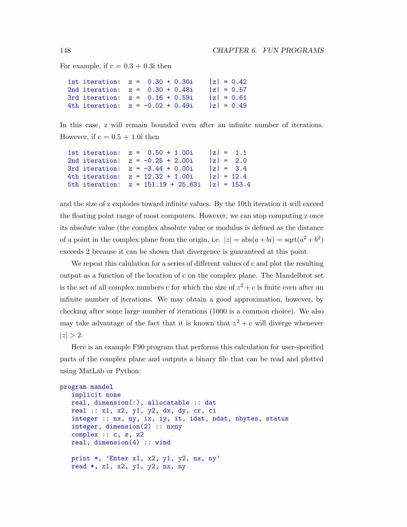
148 CHAPTER 6. FUN PROGRAMS
For example, if c = 0.3 + 0.3i then
1st iteration: z = 0.30 + 0.30i |z| = 0.422nd iteration: z = 0.30 + 0.48i |z| = 0.573rd iteration: z = 0.16 + 0.59i |z| = 0.614th iteration: z = -0.02 + 0.49i |z| = 0.49
In this case, z will remain bounded even after an infinite number of iterations.
However, if c = 0.5 + 1.0i then
1st iteration: z = 0.50 + 1.00i |z| = 1.12nd iteration: z = -0.25 + 2.00i |z| = 2.03rd iteration: z = -3.44 + 0.00i |z| = 3.44th iteration: z = 12.32 + 1.00i |z| = 12.45th iteration: z = 151.19 + 25.63i |z| = 153.4
and the size of z explodes toward infinite values. By the 10th iteration it will exceed
the floating point range of most computers. However, we can stop computing z once
its absolute value (the complex absolute value or modulus is defined as the distance
of a point in the complex plane from the origin, i.e. |z| = abs(a+ bi) = sqrt(a2 + b2)
exceeds 2 because it can be shown that divergence is guaranteed at this point.
We repeat this calulation for a series of different values of c and plot the resulting
output as a function of the location of c on the complex plane. The Mandelbrot set
is the set of all complex numbers c for which the size of z2 + c is finite even after an
infinite number of iterations. We may obtain a good approximation, however, by
checking after some large number of iterations (1000 is a common choice). We also
may take advantage of the fact that it is known that z2 + c will diverge whenever
|z| > 2.
Here is an example F90 program that performs this calculation for user-specified
parts of the complex plane and outputs a binary file that can be read and plotted
using MatLab or Python:
program mandelimplicit nonereal, dimension(:), allocatable :: datreal :: x1, x2, y1, y2, dx, dy, cr, ciinteger :: nx, ny, ix, iy, it, idat, ndat, nbytes, statusinteger, dimension(2) :: nxnycomplex :: c, z, z2real, dimension(4) :: wind
print *, ’Enter x1, x2, y1, y2, nx, ny’read *, x1, x2, y1, y2, nx, ny

6.2. FRACTALS 149
dx = (x2 - x1) / real(nx)dy = (y2 - y1) / real(ny)
allocate(dat(nx*ny))
idat=0do ix = 1, nx
do iy = 1, nycr = x1 + dx/2. + dx*real(ix-1)ci = y1 + dy/2. + dy*real(iy-1)c = cmplx(cr, ci)z = cmplx(0.0, 0.0)do it = 1, 1000
z = c + z*zif (cabs(z) > 2) exit
enddoidat = idat + 1dat(idat) = it
enddoenddoprint *, ’Finished calculation’ndat = idatprint *, ’ndat = ’,ndat
open (12, file=’fractal.bin’, form=’unformatted’)nxny(1) = nxnxny(2) = nywrite (12) nxnywind(1) = x1wind(2) = x2wind(3) = y1wind(4) = y2write (12) windwrite (12) datclose (12)
end program mandel
The program computes the result for a grid of points in the complex plane,
defined by the user-defined limits x1 and x2 for the real part and y1 and y2 for the
complex part. The number of points computed in x and y are input as nx and ny.
This will determine the resolution of the plot. For example, nx=50 and ny=50 will
result in an image 50 pixels wide by 50 pixels tall. Although the image is really
two-dimensional, I store the results in the 1-D array, dat, because this simplies the
output of the results. Notice how allocate is used to set dat to dimension(nx*ny)
on the fly.

150 CHAPTER 6. FUN PROGRAMS
The spacing in x and y are defined by:
dx = (x2 - x1) / real(nx)dy = (y2 - y1) / real(ny)
Note the conversion of the integer variables nx and ny to floats prior to performing
the division.
Here are the main loops that actually do the calculation:
idat=0do ix = 1, nx
do iy = 1, nycr = x1 + dx/2. + dx*real(ix-1)ci = y1 + dy/2. + dy*real(iy-1)c = cmplx(cr, ci)z = cmplx(0.0, 0.0)do it = 1, 1000
z = c + z*zif (cabs(z) > 2) exit
enddoidat = idat + 1dat(idat) = it
enddoenddo
The real and imaginary parts of c are set to the center of the “pixel” with sides dx
and dy. The calculation is done for a maximum of 1000 iterations. The calculation
is halted if |z| > 2 by exiting the for loop. The iteration number is saved in the dat
array, using idat as a counter.
The next step is to save this information to a file. For speed in the case of a
large dat array, we use a binary file. We create and open the file with
open (12, file=’fractal.bin’, form=’unformatted’)
We use form=’unformatted’ to specify that this is a binary file, not an ascii file.
Before writing the dat array to the file, we write some header information that
will help MatLab or Python to know the size of the array and the values of x1, x2,
y1, and y2. Writing to a binary file in Fortran is done using the write statement
without a format. We set up the 2-element int array, nxny, to handle the output of
nx and ny:
nxny(1) = nxnxny(2) = nywrite (12) nxny

6.2. FRACTALS 151
and we set up a 4-element float array, wind, to handle the output of x1, etc.
wind(1) = x1wind(2) = x2wind(3) = y1wind(4) = y2write (12) wind
Finally, we write the output array to the file
write (2) dat
For this program, it is a good idea to compile with the -O compiler option to
make it run faster:
gfortran -O mandel.f90 -o mandel
The Mandelbrot set is approximated in our program by places on the complex
plane where the output value (contained in the dat array) is 1000, i.e., the z function
has not diverged even after 1000 iterations. Output values less than 1000 provide a
message of how quickly the function diverges (small values indicate rapid divergence,
larger values indicate slower divergence). Plots of the output usually use colors to
indicate the different output values.
6.2.1 Plotting using MatLab
Here is how to plot our output using Matlab:
clf resetclear[fid, message] = fopen(’fractal.bin’)
% Fortran I/O has extra four bytes at beginning and end of writes[dum, count] = fread(fid, [1], ’int’);[size, count] = fread(fid, [2], ’int’);[dum, count] = fread(fid, [1], ’int’);
nx = size(1)ny = size(2)
[dum, count] = fread(fid, [1], ’int’);[wind, count] = fread(fid, [4], ’float’)[dum, count] = fread(fid, [1], ’int’);
x1 = wind(1)

152 CHAPTER 6. FUN PROGRAMS
x2 = wind(2)y1 = wind(3)y2 = wind(4)
[dum, count] = fread(fid, [1], ’int’);[z, count] = fread(fid, [nx,ny], ’float’);fclose(fid);
z2 = log10(z);axis( [x1, x2, y1, y2] ); axis(’square’); hold on;imagesc( [x1, x2], [y1, y2], z2 );colorbar;
One important detail is that Fortran (unlike C) writes an extra 4 bytes before
and after each of the binary writes. So we need to read these extra btyes with our
Matlab script into a dummy variable or we will not be properly aligned with the
data fields.
We set the output array to z and use imagesc to plot the result using the default
color scheme. We plot log(z) rather than z because it shows some of the details a
little better.
6.2.2 Plotting using Python
Here is one way to plot our output using Python, a script called plotfractal.py
#! /usr/bin/env pythonimport numpy as npfrom scipy.io import FortranFileimport matplotlibmatplotlib.use("TkAgg")import pylab
# Open the Fortran unformatted binaryf = FortranFile(’fractal.bin’, ’r’)
# Read the contents from fractal.bin in the order that they were written# Read nx, ny[nx, ny] = f.read_ints(np.int32)print ’nx, ny = ’, nx, ny# Read windwind = f.read_record(’float32’)x1 = wind[0]x2 = wind[1]y1 = wind[2]y2 = wind[3]print ’x1,x2,y1,y2 =’, x1, x2, y1, y2# Read dat, then reshape into a 2D array Z for plotting (need to do transpose)

6.2. FRACTALS 153
dat = f.read_record(’float32’)Z = np.transpose(dat.reshape(nx,ny))
# Construct the x and y vectors for plottingdx = (x2 - x1)/nxdy = (y2 - y1)/nyx = np.arange(x1 + dx/2., x2, dx)y = np.arange(y1 + dy/2., y2, dy)
# plotpylab.pcolormesh(x,y,np.log10(Z),cmap=’jet’)pylab.xlabel(’x’, fontsize=16)pylab.ylabel(’y’, fontsize=16)pylab.colorbar()pylab.show()
I got this script from Robin Matoza at UCSB and it works more cleanly than an
older Python script I had kludged together. It takes advantage of the scipy.io.FortranFile
method for reading Fortran unformatted binary files (see https://docs.scipy.org/doc/scipy-
0.16.0/reference/generated/scipy.io.FortranFile.html) This has the advantage that
it knows about the extra 4 bytes that Fortran puts before and after every binary-
write, so we do not need to explicitly read these, as we did in the Matlab script
above.
Most of the script should be self-explanatory. Note how we read in the wind
array and then assign the plot limits:
wind = f.read_record(’float32’)x1 = wind[0]x2 = wind[1]y1 = wind[2]y2 = wind[3]
We read in the big vector containing the data for the image and then reshape it intothe correct matrix form for plotting:
dat = f.read_record(’float32’)Z = np.transpose(dat.reshape(nx,ny))
Next, we compute dx and dy and set up the x and y vectors for plotting:
dx = (x2 - x1)/nxdy = (y2 - y1)/nyx = np.arange(x1 + dx/2., x2, dx)y = np.arange(y1 + dy/2., y2, dy)
Note that the last value of x will be x2 - dx/2.
The plot looks nicer if we take the log before plotting. The ’jet’ color scheme is
a good choice.

154 CHAPTER 6. FUN PROGRAMS
pylab.pcolormesh(x,y,np.log10(Z),cmap=’jet’)
It’s fun to explore the effect of different color maps in Python. Here is a site that
shows lots of them: http://www.scipy.org/Cookbook/Matplotlib/Show colormaps
6.2.3 Good targets and more about fractals
The entire Mandelbrot set may be imaged in the window
real -2 to 0.5, imag -1.25 to 1.25 (i.e., -2, 0.5, -1.25, 1.25)
It is also fun to zoom in on details of the image. Here are some suggestions for
places to look:
-0.95 -0.90 0.25 0.30-0.75 -0.65 0.25 0.35-0.73 -0.72 0.282 0.292-0.703 -0.693 0.26 0.27
Further details about generating fractals may be found in a series of articles by
A.K. Dewdney in the Computer Recreations section that used to appear in Scientific
American. The August 1985 article describes the Mandelbrot set, the November
1987 article talks about the related Julia sets, and the July 1989 article is about
fractals called “biomorphs” that look like little creatures. There are also lots of
books on fractals that have many beautiful images.
The study of fractals is related to chaos theory and the fact that in physical
systems (weather is one example) are inherently unpredictable on large time scales
because small perturbations to the starting conditions will cause large changes over
time.
ASSIGNMENT FRAC1
Rewrite the mandel.c and plotfractal.m (or plotfractal.py) programs to plot ex-
amples of the Julia sets and the biomorphs. You will want to first read the appro-
priate Scientific American articles.
1. Produce PDF files of 3 especially nice images of Julia sets.
2. Reproduce and make images of as many of the biomorphs as you can that are
shown on p. 110 of the biomorph article.

6.3. FUN WITH SPECTRA 155
Part (2) is harder because you will have to generate more complicated complex
functions than those that are used for the Mandelbrot and Julia sets. You may have
to consult a book on complex numbers to find suitable formulae to compute sin(z),
zz, etc.
Please e-mail me the PDF files and copies of your F90 and Matlab or Python
source code.
Have fun!
6.3 Fun with spectra
Computing Fourier transforms using the Fast Fourier Transform (FFT) algorithm
is a standard tool in geophysical analysis. There are many books and articles on
Fourier theory and how the FFT works. I am distributing the part of Numerical
Recipes that discusses this, which seems as good a treatment as any. You will
certainly learn much more about this if you take our Data Analysis class.
For brevity in this class I am simply going to focus on what you need to know
to use an FFT program and leave the theory for you to pick up elsewhere.
We start with a “time series,” which is a series of measurements that are made
at some regular interval. These measurements are normally stored on the computer
in an array. We also need to know the sample interval (the time between sample
points, the reciprocal of the digitization rate) and the number of points in the time
series. In most cases the time series consists of real (i.e., not complex) numbers and
we will assume this is true for the examples shown.
The purpose of the FFT is to examine the different frequency waves that may be
present in the data. The FFT is a linear transformation that allows us to look at the
data in the “frequency domain” rather than the “time domain” of the original data.
In fact, the original time series can be expressed exactly as a sum of harmonic waves
of different frequency content and phase. The FFT allows us to readily compute
what the frequencies and phases of these waves are.
The simplest FFT algorithms require that the number of points in the original
time series be a power of two. We will assume that this is true here, but you should
be aware that alternative FFT methods exist for non-powers of two.
Thus, the input to a typical FFT algorithm will consist of an array of data values,
the number of time points (n), and the sample interval (dt). For a real time series,
the FFT algorithm will then return a complex spectra that will give the amplitude

156 CHAPTER 6. FUN PROGRAMS
and phase at a series of equally spaced frequency points. There will be n/2 + 1
frequency points and the frequency spacing will be df = 1/(n ∗ dt).
The first frequency point is at f = 0.0
The last frequency point is at f = 1/(2∗dt) and is called the Nyquist frequency.
The Nyquist frequency is the highest frequency that one can resolve in the time
series. At the Nyquist frequency, there are two data points in the time series per
wavelength. If higher frequencies are present in the data, they will be “aliased” so
that they are seen at lower frequencies. From the time series alone, there is no way
to discriminate between correctly resolved frequencies and aliased data from higher
frequencies. Thus, sometimes filters (anti-aliasing filters) are applied to the data
prior to digitization to remove the frequencies above the Nyquist so that this will
not be a problem.
The FFT algorithm provides the spectra at n/2 + 1 frequency points which may
be represented as n/2 + 1 complex numbers. (complex numbers are necessary to
represent both the amplitude and phase of each harmonic component).
“Wait a minute,” the alert reader might cry. We started with n real points in
the time domain and now we have n+ 2 real points in the frequency domain, if we
count each complex number as two reals. Have we gained information compared
to the original time series? The resolution to this apparent problem comes from
the fact that the first and last frequency points always have zero imaginary parts.
Thus the total number of independent data points is the same in both the time and
frequency domains. In fact, most FFT algorithms return only n/2 frequency points
by packing the real part of the Nyquist point into the imaginary part of the zero
frequency point.
Once we have the frequency domain points we can make an amplitude spectra
plot by plotting the absolute values (Cabs function) of the points versus frequency.
If we want a power spectrum, then we square the amplitudes. Getting the correct
units on the y-axis can be a tricky business (let’s save that discussion until your
time series analysis class); in many cases, however, we are only interested in the
position of the peaks or the shape of the spectrum so we don’t need to worry about
this.
We can also transform back to the time domain by computing an inverse FFT.
If your code is working correctly, you should get back exactly the same time series
as you started with.
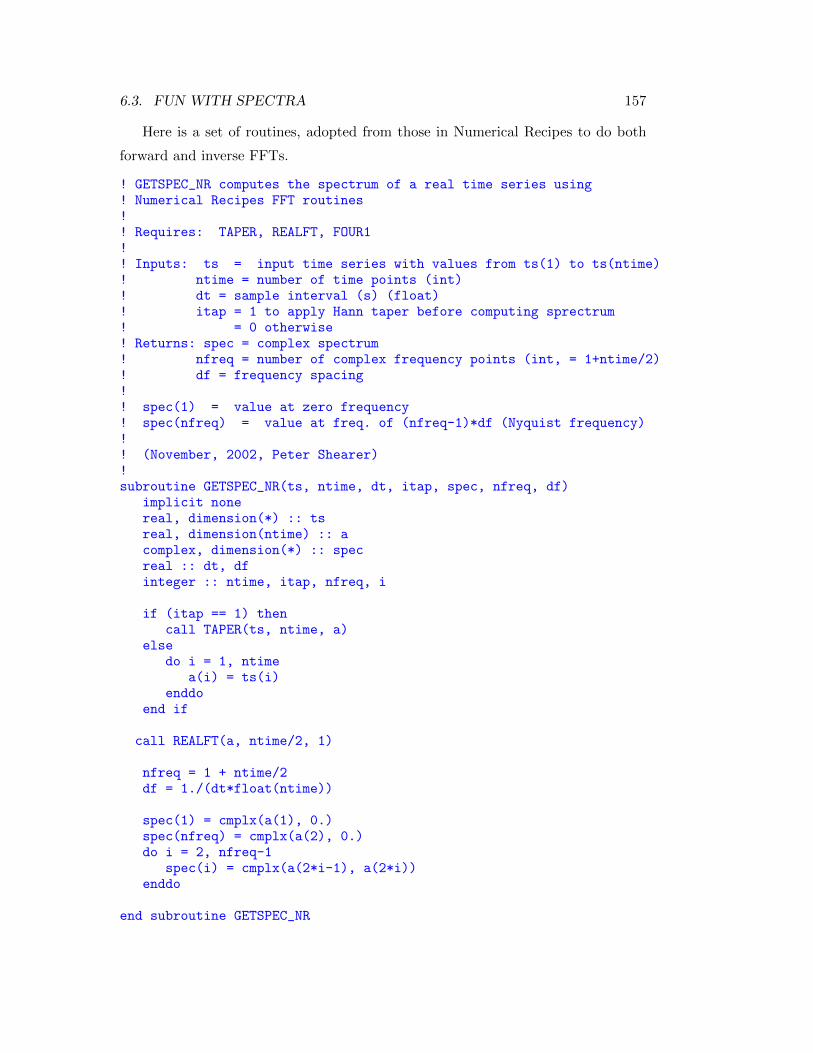
6.3. FUN WITH SPECTRA 157
Here is a set of routines, adopted from those in Numerical Recipes to do both
forward and inverse FFTs.
! GETSPEC_NR computes the spectrum of a real time series using! Numerical Recipes FFT routines!! Requires: TAPER, REALFT, FOUR1!! Inputs: ts = input time series with values from ts(1) to ts(ntime)! ntime = number of time points (int)! dt = sample interval (s) (float)! itap = 1 to apply Hann taper before computing sprectrum! = 0 otherwise! Returns: spec = complex spectrum! nfreq = number of complex frequency points (int, = 1+ntime/2)! df = frequency spacing!! spec(1) = value at zero frequency! spec(nfreq) = value at freq. of (nfreq-1)*df (Nyquist frequency)!! (November, 2002, Peter Shearer)!subroutine GETSPEC_NR(ts, ntime, dt, itap, spec, nfreq, df)
implicit nonereal, dimension(*) :: tsreal, dimension(ntime) :: acomplex, dimension(*) :: specreal :: dt, dfinteger :: ntime, itap, nfreq, i
if (itap == 1) thencall TAPER(ts, ntime, a)
elsedo i = 1, ntime
a(i) = ts(i)enddo
end if
call REALFT(a, ntime/2, 1)
nfreq = 1 + ntime/2df = 1./(dt*float(ntime))
spec(1) = cmplx(a(1), 0.)spec(nfreq) = cmplx(a(2), 0.)do i = 2, nfreq-1
spec(i) = cmplx(a(2*i-1), a(2*i))enddo
end subroutine GETSPEC_NR

158 CHAPTER 6. FUN PROGRAMS
! GETTS_NR computes a real time series from a complex spectrum! (stored as in GETSPEC_NR) using Numerical Recipes FFT routines!! Requires: REALFT, FOUR1!! Inputs: spec = complex spectrum stored as floats! nfreq = number of complex frequency points (int, = 1+ntime/2)! df = frequency spacing!! Returns: ts = input time series with values from ts(1) to ts(ntime)! ntime = number of time points (int)! dt = sample interval (s) (float)!! spec(1) = value at zero frequency! spec(nfreq) = value at freq. of (nfreq-1)*df (Nyquist frequency)!! (November, 2002, Peter Shearer)!subroutine GETTS_NR(spec, nfreq, df, ts, ntime, dt)
real, dimension(*) :: tsreal, dimension(ntime+2) :: acomplex, dimension(*) :: specreal :: df, dt, scaleinteger :: nfreq, ntime, n, isign, i
ntime = (nfreq-1)*2dt = 1./(df*float(ntime))scale = 2.0/float(ntime)
a(1) = real(spec(1))*scalea(2) = real(spec(nfreq))*scale
do i = 2, nfreq-1a(2*i-1) = real(spec(i))*scalea(2*i) = aimag(spec(i))*scale
enddo
call REALFT(a, ntime/2, -1)
do i = 1, ntimets(i) = a(i)
enddo
end subroutine GETTS_NR
! TAPER multiplies ts1 for Hann taper and puts result in ts2!subroutine TAPER(ts1, n, ts2)

6.3. FUN WITH SPECTRA 159
implicit nonereal, dimension(n) :: ts1, ts2real :: pihalf, tsmid, frac, angle, tapinteger :: n, i, i2pihalf = 3.1415927/2.i2 = n/2 +1tsmid = float(n)/2. + 0.5do i = 1, i2
frac = float(i)/tsmidangle = pihalf*fractap = sin(angle)**2ts2(i) = ts1(i)*tapts2(n+1-i) = ts1(n+1-i)*tap
enddoend subroutine TAPER
SUBROUTINE REALFT(DATA,N,ISIGN)REAL*8 WR,WI,WPR,WPI,WTEMP,THETADIMENSION DATA(*)THETA=6.28318530717959D0/2.0D0/DBLE(N)C1=0.5IF (ISIGN.EQ.1) THEN
C2=-0.5CALL FOUR1(DATA,N,+1)
ELSEC2=0.5THETA=-THETA
ENDIFWPR=-2.0D0*DSIN(0.5D0*THETA)**2WPI=DSIN(THETA)WR=1.0D0+WPRWI=WPIN2P3=2*N+3DO 11 I=2,N/2+1
I1=2*I-1I2=I1+1I3=N2P3-I2I4=I3+1WRS=SNGL(WR)WIS=SNGL(WI)H1R=C1*(DATA(I1)+DATA(I3))H1I=C1*(DATA(I2)-DATA(I4))H2R=-C2*(DATA(I2)+DATA(I4))H2I=C2*(DATA(I1)-DATA(I3))DATA(I1)=H1R+WRS*H2R-WIS*H2IDATA(I2)=H1I+WRS*H2I+WIS*H2RDATA(I3)=H1R-WRS*H2R+WIS*H2IDATA(I4)=-H1I+WRS*H2I+WIS*H2RWTEMP=WRWR=WR*WPR-WI*WPI+WR

160 CHAPTER 6. FUN PROGRAMS
WI=WI*WPR+WTEMP*WPI+WI11 CONTINUE
IF (ISIGN.EQ.1) THENH1R=DATA(1)DATA(1)=H1R+DATA(2)DATA(2)=H1R-DATA(2)
ELSEH1R=DATA(1)DATA(1)=C1*(H1R+DATA(2))DATA(2)=C1*(H1R-DATA(2))CALL FOUR1(DATA,N,-1)
ENDIFRETURNEND
SUBROUTINE FOUR1(DATA,NN,ISIGN)REAL*8 WR,WI,WPR,WPI,WTEMP,THETADIMENSION DATA(*)N=2*NNJ=1DO 11 I=1,N,2
IF(J.GT.I)THENTEMPR=DATA(J)TEMPI=DATA(J+1)DATA(J)=DATA(I)DATA(J+1)=DATA(I+1)DATA(I)=TEMPRDATA(I+1)=TEMPI
ENDIFM=N/2
1 IF ((M.GE.2).AND.(J.GT.M)) THENJ=J-MM=M/2
GO TO 1ENDIFJ=J+M
11 CONTINUEMMAX=2
2 IF (N.GT.MMAX) THENISTEP=2*MMAXTHETA=6.28318530717959D0/(ISIGN*MMAX)WPR=-2.D0*DSIN(0.5D0*THETA)**2WPI=DSIN(THETA)WR=1.D0WI=0.D0DO 13 M=1,MMAX,2DO 12 I=M,N,ISTEP
J=I+MMAXTEMPR=SNGL(WR)*DATA(J)-SNGL(WI)*DATA(J+1)TEMPI=SNGL(WR)*DATA(J+1)+SNGL(WI)*DATA(J)

6.3. FUN WITH SPECTRA 161
DATA(J)=DATA(I)-TEMPRDATA(J+1)=DATA(I+1)-TEMPIDATA(I)=DATA(I)+TEMPRDATA(I+1)=DATA(I+1)+TEMPI
12 CONTINUEWTEMP=WRWR=WR*WPR-WI*WPI+WRWI=WI*WPR+WTEMP*WPI+WI
13 CONTINUEMMAX=ISTEP
GO TO 2ENDIFRETURNEND
GETSPEC NR, GETTS NR and TAPER are my own inventions; REALFT
and FOUR1 are from Numerical Recipes. Hopefully the documentation for GET-
SPEC NR and GETTS NR is self-explanatory.
The GETSPEC NR function includes an option to multiply the time series by
a cos**2 function (i.e., Hanning taper) before computing the FFT. This generally
improves the appearence of the spectrum and avoids artifacts that may result from
the abrupt truncation of the time series at the end of the data window.
A typical call to GETSPECNR would have the form:
call GETSPEC_NR(a, n, dt, itap, b, nfreq, df)
where a is the data array. You should define the sizes of a and b in the calling
program as, for example:
integer, parameter :: maxpts = 8192real, dimension(maxpts) :: acomplex, dimension(maxpts/2+1) :: b
WARNING: The routines do not check if n is a power of two. This would be a
useful improvement to make the routines more robust with respect to user errors in
the calling program.
6.3.1 Guitar string example
A properly tuned guitar will have strings with fundamental mode frequencies as
follows: E = 82 Hz, A = 110 Hz, D = 147 Hz, G = 196 Hz, B = 247 Hz, E = 330
Hz.

162 CHAPTER 6. FUN PROGRAMS
There will be overtones (harmonics) at frequencies of n*f0 where f0 is the
fundamental (lowest) frequency. Thus, for the A string, we should expect to see
peaks at 110 Hz, 220 Hz, 330 Hz, 440 Hz, etc. The relative power between the
different harmonics is what determines the tone of the guitar.
Unfortunately, the MacCRO program mentioned in the next paragraph does not
seem to work/exist for modern Macs. Until I find a suitable replacement program,
I will just have to use some files that I previously digitized.
The shareware program MacCRO (http://pderrin.cjb.net/ maccro.html) uses
the audio input on the Mac to simulate an oscilloscope. For our purposes, its most
useful feature is the ability to download digitized sounds to a file. For a class demo,
my plan is to use the program to digitize the sound of the A string, save the result
to a file, and then bring the file over to the Sun where it can be FFTed and the
resulting spectrum plotted.
If we have time, it will be interesting to compare:
(1) string plucked near center vs. near one end
(2) sound sampled just after pluck vs. a few seconds later
(3) cheap vs. expensive guitar ———————————————————-
Assuming we have a digitized ascii time series file (one point per line) with a
header line for the sample rate, here is a program to read the data, compute the
FFT, and output the spectrum:
! program to compute spectrum of MacCRO output fileprogram macfft
implicit noneinteger, parameter :: maxpts = 8192real, dimension(maxpts) :: a, a2complex, dimension(maxpts/2+1) :: breal :: x, y, dt, df, samrat, samcount, freq, ampinteger :: ios, i, j, idir, itap=0, n, nfreq, nn, menucharacter (len=100) :: infile, linebuf, outfilecharacter (len=20) :: word1, word2
print *, ’Enter input file name from MacCRO program’read *, infileopen (11, file=infile, status=’old’)
read (11, ’(a)’) linebufprint *, ’First line of file = ’, linebufread (11, *) word1, word2, samratdt = 1.0/samratprint *, ’samrat, dt = ’, samrat, dtread (11, *) word1, word2, samcount

6.3. FUN WITH SPECTRA 163
print *, ’samcount = ’, samcountread (11, ’(a)’) linebuf
do i = 1, 10000read (11, *, iostat=ios) xif (ios < 0) exita(i) = x
enddon = i - 1print *, ’ n= ’,ndo i = 1, 5print *, i, a(i)
enddo
print *, ’Enter desired power of two’read *, nnn = nn
print *, ’Apply Hann taper? (0) no, (1) yes’read *, itap
call GETSPEC_NR(a, n, dt, itap, b, nfreq, df)print *, ’nfreq, df = ’, nfreq, df
print *, ’Output spectrum to: (1) screen or (2) file’read *, menuif (menu.eq.2) then
print *, ’Enter file name’read *, outfileopen (12, file=outfile)
end if
do i = 1, nfreqfreq = float(i-1)*dfamp = cabs(b(i))if (menu == 1) then
print ’(4f10.4)’, freq, amp, real(b(i)), aimag(b(i))else
write (12, ’(4f10.4)’) freq, amp, real(b(i)), aimag(b(i))end if
enddo
end program macfft
We can then plot the spectrum using plotxy or another plotting program. In
the case of the guitar string, the fundamental frequency will be the lowest frequency
peak in the spectrum and the harmonics will be evenly spaced peaks in frequency
going to higher frequencies. By plucking the string in different places, it is possible
to excite the harmonics more than the fundamental mode.

164 CHAPTER 6. FUN PROGRAMS
6.3.2 ASSIGNMENT FFT1
Get the file bfo1 from the class website. This is a time series of the 1994 deep Bolivian
earthquake as recorded at Black Forest Observatory, Germany (48.3319N,8.3311E).
The sample interval is 40 s and there are 24225 points in the file, representing over
11 days of data. The sensor is vertical in orientation so primarily spheroidal modes
are recorded.
(a) Plot the time series using whatever plotting program you want. Label the
x-axis in units of hours.
(b) Write a F90 program to read the data and compute the spectrum, both with
and without first applying a Hann taper.
(c) Make nice plots of the spectra that compare the results with and without
the Hann taper. Label the x-axis in units of mHz. Make plots that go from zero to
the Nyquist frequency and also some closeups from zero to 2 mHz.
(d) Using Table V from the PREM paper (Dziewonski and Anderson, PEPI 25,
297-356, 1981, see me if you want to make a copy), identify and label as many of
the peaks below 2 mHz as you can.
NOTE: 24225 is not a power of two. You have two choices. You can ei-
ther truncate the time series at 2**14=16384 or pad the time series with zeros
to 2**15=32768. In the latter case, make sure you apply the taper to the 24225-
point series and THEN pad with zeros (i.e., you can’t just use the taper option in
getspec).