2 basic statistics - igpp home page · 2007-02-11 · 2 basic statistics: 2.1 introduction 2.1.1...
TRANSCRIPT

Created by Robert L. McPherron Created on 10/16/2001 11:15 AM Printed: February 11, 2007
2 Basic Statistics:
2.1 Introduction
2.1.1 The role of this chapter Virtually every method discussed in this book utilizes basic statistical procedures in some way. This chapter reviews some of these concepts introducing their definitions and illustrating their application with simple examples. The chapter emphasizes properties of a univariate time series that do not depend on the temporal order of the data. Chapter 3 generalizes these ideas to multivariate time series. Most of our examples use long time series of magnetic indices and solar wind data. Later chapters extend the presentation to methods dependent on the order of data points. The statistical quantities and their graphical displays were produced using a widely available software package and its statistical toolbox. Our emphasis in this chapter is on some of the problems and pitfalls of applying these definitions to typical space physics data.
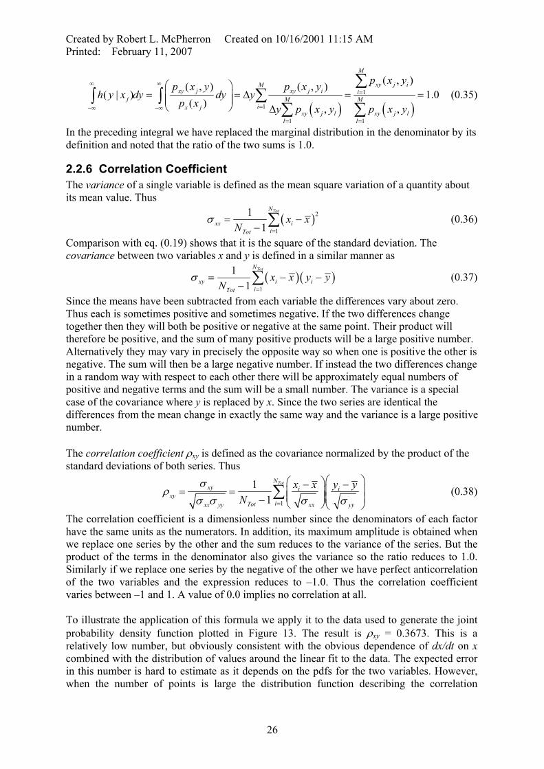
2.1.2 Organization of this Chapter We begin Chapter 2 with a description of the various data types used in our illustrations. We then present the concept of the probability density function (pdf) of a single variable. We next define a number of statistical measures derived from the pdf and show different ways of calculating and displaying this function graphically. The normal or Gaussian pdf is discussed and its importance in statistics emphasized. We then consider the problem of estimating errors in the pdf and quantities derived from it when the pdf is not Gaussian. The bootstrap method is described as an empirical technique for making such error estimates. We next consider the integral of the pdf, the cumulative distribution function (cdf). The Kolmogorov-Smirnov (K-S) test is introduced as a simple means for comparing two cdfs to decide whether they represent two different samples of the same parent population. We then turn to the joint probability distribution function between two variables and introduce the concepts of conditional probability distributions and marginal distributions. We close the chapter by defining the correlation coefficient between two variables and relating it to the problem of linear regression.
2.1.3 Relation of this Chapter to Part 2 The methods described in this chapter are used many times in the second half of this book. For example, ……?????
2.1.4 The Kp and Dst Indices The Kp index is a measure of the strength of geomagnetic variations with period shorter than 3 hours caused mainly by magnetospheric substorms. The index is roughly proportional to the logarithm of the range of deviation of the most disturbed horizontal component of the magnetic field from a quiet day in a 3-hr interval [Mayaud, 1980]. Kp is one of the most commonly used indices in space physics and it is important because of the many correlations established between it and other phenomena. Kp is available continuously from the beginning of 1932. It is dimensionless and quantized in multiples of 1/3. Its range is finite and limited to the interval [0, 9]. In the following section Kp is one of time series we use to illustrate some commonly used statistical techniques.
1

Created by Robert L. McPherron Created on 10/16/2001 11:15 AM Printed: February 11, 2007
10/17 10/24 10/31 11/070
3
6
Kp In
dex
3-HOUR Kp INDEX DURING OCTOBER 1999
10/17 10/24 10/31 11/07-250-200-150-100-50
050
Date in 1999
Dst
Inde
x (n
T)
1-HOUR Dst INDEX DURING OCTOBER 1999
Figure 1. The Kp and Dst indices of magnetic activity during a magnetic storm in October 1999. Kp has 3-hour resolution and primarily measures disturbances caused by ionospheric currents in the auroral zone. The Dst index has 1-hour resolution. It measures the strength of the current produced by particles drifting around the earth at radial distances of 3-8 Re.
The first step in the analysis of any time series is to plot and examine the data. Many of the characteristics and problems with the data are immediately obvious in such plots. For example, the time variations in Kp during a magnetic storm are presented in the top panel of Figure 1. The stair-step nature of the plot reveals that Kp is quantized both in amplitude and time. On October 19, 15-18 UT magnetic activity was at an extremely quiet level with Kp = 0. During the next four days it rose to an extremely disturbed level of Kp = 8, a value close to the maximum allowable. Following the peak disturbance activity gradually decreased throughout the following week. The Dst (disturbance storm time) index is a measure of the strength of the ring current created by the drifts of charged particles in the earth’s magnetic field. This index is the average of the hourly deviation of the H component of the magnetic field measured by several stations around the earth [Sugiura, 1964; Sugiura and Kamei, 1991]. A rapid decrease in Dst is an indication that the ring current is growing, and that a magnetic storm is in progress. Ideally Dst is linearly proportional to the total energy of the drifting particles. The standard Dst index calculated at hourly resolution from 4-5 stations, and quantized to 1 nT, is available continuously since 1957. A higher resolution version of the Dst index called Sym-H is calculated using a slightly different procedure with one-minute resolution [Araki et al., 1990]. Sym-H index is available since 1984. A plot of the standard 1-hour resolution Dst index is plotted in the bottom panel of Figure 1. At the time Kp = 0 the Dst index was also approaching zero. About a day later the beginning of the magnetic storm is evident from the sharp increase that occurred in hour 02 of October 21. The initial phase of the magnetic storm
2

Created by Robert L. McPherron Created on 10/16/2001 11:15 AM Printed: February 11, 2007
during which Dst is elevated relative to values prior to the storm persisted until hour 17. In hour 17 a rapid decrease in Dst indicates that the main phase of the storm was in progress. The storm reached its minimum value of –231 nT in hour 06 of October 22 and then began to recover. The recovery phase consisted of two stages - a rapid recovery for ~17 hours, and then a prolonged, slow recovery for many days. The correlation between the high Kp index and the rapid decrease is Dst is obvious.
2.1.5 Data Formats The Kp and Dst indices can be obtained via the Internet from various data centers as for example WDC-A at NOAA in Boulder, CO: http://www.ngdc.noaa.gov/stp/stp.htmlData downloaded from this or other data centers is usually organized in the World Data Center Exchange format. Any attempt to work with the variants of this format will quickly convince the user of the value of plain text flat files. For this book we have reformatted the original data files into two-column tables with decimal day number (where 1.00 corresponds to 1-Jan-0000) in column 1, and the index in column 2. To reduce storage the values in the WDC format for Kp are rounded to the nearest 1/10 unit and saved as integer tenth units, for example the values [1+1/3, 2-1/3, 3] become [13, 17, 30]. This rounding slightly affects the values of various statistical properties if not corrected. Worse, it radically affects the appearance of probability density functions unless special care is taken with the definition of bins. The Dst index is rounded to the nearest nanotesla, but its range is so large relative to this resolution that quantization does not normally affect the binning required for the creation of a pdf.
2.2 Statistical Properties of a Data Set Today almost all data are digital in form. Continuous time series such as the voltage output of a sensor are represented by a finite set of equally spaced values of finite precision. The process of converting the sensor output to this form is called sampling the signal. Sampling introduces a number of errors into the data that we briefly describe below. The output of this procedure is usually called a time series, although the independent variable may be any physical variable such as distance or temperature. In this chapter we consider only those properties of a time series that are independent of the order of the values. The mean value is an example of such a quantity. Our discussion applies equally well to any collection of values however produced, as for example the weights of students in a given classroom. Clearly the table of measured weights has a mean value, but the order in which students are weighted and listed in the table is unimportant.
2.2.1 Quantization, Dynamic Range, Discretization, Windowing Quantization is the process of converting an analog signal such as the voltage output from an amplifier to a number with finite precision. For example, suppose the voltage is limited to the range ±10 Volts and the signal is converted to an integer number of Volts. Then there are only 21 possible values for the voltage. If instead the conversion is in ½-Volt steps there will be 41 possible values. A plot of the quantized data will be a stair-step function as illustrated in Figure 2. The process of quantization introduces noise into the signal. Sometimes the nearest step is above the current value of the signal, and sometimes it is below. The maximum possible error is ±δA/2, where δA is the difference between successive quantized values. Later we show that the rms error due to quantization is 1/(12* δA). The upper and lower limits of a signal are usually imposed by the electronics that convert the physical variable to an electrical signal. Typically these limits represent the extreme voltages that can
3

Created by Robert L. McPherron Created on 10/16/2001 11:15 AM Printed: February 11, 2007
Upper
Lower
Quantization
SaturationOutlier
∆t
Time
Dyn
am
ic R
ang
e
Figure 2. A schematic illustration of the process of sampling data.
be provided by a power supply. These limits define the dynamic range of the instrument. If the physical quantity takes on a value beyond the dynamic range the measured voltage will saturate, i.e. become fixed at the power supply voltage. Saturation introduces errors into the resulting sequence of values whose effects depend on the nature of the signal and how often it occurs. The process of quantization is almost always associated with discretization. Discretization is the process of converting a continuous signal to a time sequence of instantaneous samples. Usually the successive samples are equally spaced with a time separation ∆t called the sample interval. Discretization introduces errors into the data when variations with period shorter than half the sampling period are present. These errors are usually called aliasing. For a discussion of these errors see Section ??? in Chapter ??? Together the two processes are called sampling the signal. A third step in sampling a signal is to limit the number of samples to a finite time interval starting and ending at fixed times. This step is usually referred to as windowing the data. This process is equivalent to multiplying an infinite sequence of samples by a function that has the value zero outside the window and one inside the window. Windowing also introduces distortion into the data that are discussed in Section ??? of Chapter ???? We emphasize that the basic statistical properties described in this chapter do not depend on the order in which the measurements are made. However, they do depend on the manner in which the sample values are distributed within the dynamic range of the measurement.
2.2.2 Invariance of Statistical Properties An important question to be asked about any statistical quantity is whether it is the same for different samples of the population. For example, suppose the parent population is all third grade students in the United States. One could measure the weight of all of these students and group the measurements by state. Then, for each state, determine the mean weight of students and sort the means into increasing order. The question is whether the differences in the mean values are larger than expected by chance, or whether they represent differences in diet between the states. Alternatively, we could randomly select groups of equal size from the
4
Created by Robert L. McPherron Created on 10/16/2001 11:15 AM Printed: February 11, 2007
entire US and determine the means of these groups. In this case it is unlikely that there would be any real differences. Then the mean value would be an invariant property of the groups. This concept of invariance of statistical properties becomes particularly important later when we consider time series. Most of our analysis techniques are based on the concept of stationarity that can be roughly defined as no change in the basic statistical properties with time. For a more formal definition see Section ???? of Chapter /??
2.2.3 The Probability Density Function (pdf) Long time series such as those provided by the Kp and Dst indices, or large tables such as the weights of third grade students, can be described by a number of statistical properties. One of the most basic properties is the probability density function or pdf. The pdf describes the probability that a single sample of a variable taken from a large sequence of observations will have a specific value. The pdf can be characterized by various moments. Moments are defined as weighted averages over the distribution of various powers of the variable. The first moment is the mean and the second moment the variance of the data. Higher order moments provide information about the asymmetry and shape of the distribution.
2.2.3.1 Formal Definition of the Probability Density Function Suppose we have a sample set of Ntot observations of some variable x. The probability density function (pdf) for this variable at the point xi is defined as
0
ˆ ( ) lim i ii x
tot
N[x ,x ∆x]p xN ∆x∆ →
⎛ ⎞+= ⎜
⎝ ⎠⎟ (0.1)
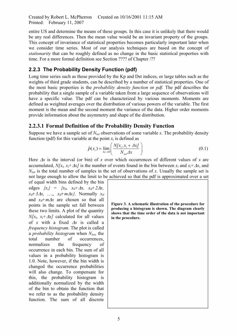
Here ∆x is the interval (or bin) of x over which occurrences of different values of x are accumulated, N[xi, xi+∆x] is the number of events found in the bin between xi and xi+∆x, and Ntot is the total number of samples in the set of observations of x. Usually the sample set is not large enough to allow the limit to be achieved so that the pdf is approximated over a set of equal width bins defined by the bin edges {xi} = {x0, x0+∆x, x0+2∆x, x0+3∆x, …,, x0+m∆x}. Normally x0 and x0+m∆x are chosen so that all points in the sample set fall between these two limits. A plot of the quantity N[xi, xi+∆x] calculated for all values of x with a fixed ∆x is called a frequency histogram. The plot is called a probability histogram when Ntot, the total number of occurrences, normalizes the frequency of occurrence in each bin. The sum of all values in a probability histogram is 1.0. Note, however, if the bin width is changed the occurrence probabilities will also change. To compensate for this, the probability histogram is additionally normalized by the width of the bin to obtain the function that we refer to as the probability density function. The sum of all discrete
Figure 3. A schematic illustration of the procedure for producing a histogram is shown. The diagram clearly shows that the time order of the data is not important in the procedure.
5
Created by Robert L. McPherron Created on 10/16/2001 11:15 AM Printed: February 11, 2007
values in the probability density distribution equals 1/∆x. The bin width ∆x is usually fixed, but in cases where some bins have very low occurrence probability it may be necessary to increase ∆x as a function of x. This procedure is summarized schematically in Figure 3. A portion of the Dst time series from Figure 1 has been rotated 90° so that the time axis is vertical and the amplitude axis is horizontal. Thin vertical lines parallel to the time axis denote wide bins in the value of the index. Discrete values of Dst are projected onto the amplitude axis and the total number falling into each bin is counted and represented by the histogram at the bottom. It is obvious that contributions to a bin can come from any time irrespective of the order of points in the time series. The pdf defined by eq. 1 satisfies the constraint that the total area under the integral of is 1.0, i.e.
ˆ ( )p x
1
ˆ1 ( ) (totN
ii
)p x dx x p x∞
−∞=
= ≅ ∆ ∑∫ (0.2)
Note that the integral may be evaluated by a simple sum provided one keeps track of the bin width used in approximating the pdf. Since the sum alone equals 1/∆x, its product with ∆x is 1.0.
0 3 6 90
0.1
0.20
0.30
Kp Index
Prob
Dis
t Fun
ctio
n
Kp PDF FOR 1932-1999
Kp=1/3Npts=198,696
0 3 6 9-3
-2
-1
0
Kp Index
Log
Prob
ablit
y
Kp PDF FOR 1932-1999
-150-100-500500
0.01
0.02
Dst Index
Dst PDF FOR 1957-1999
Dst= 10 nTNpts=376,128
-500-400-300-200-1000100-7
-6
-5
-4
-3
-2
-1
Dst Index
Log
Prob
ablit
y
∆
∆
Prob
Dis
t Fun
ctio
n
Dst PDF FOR 1957-1999
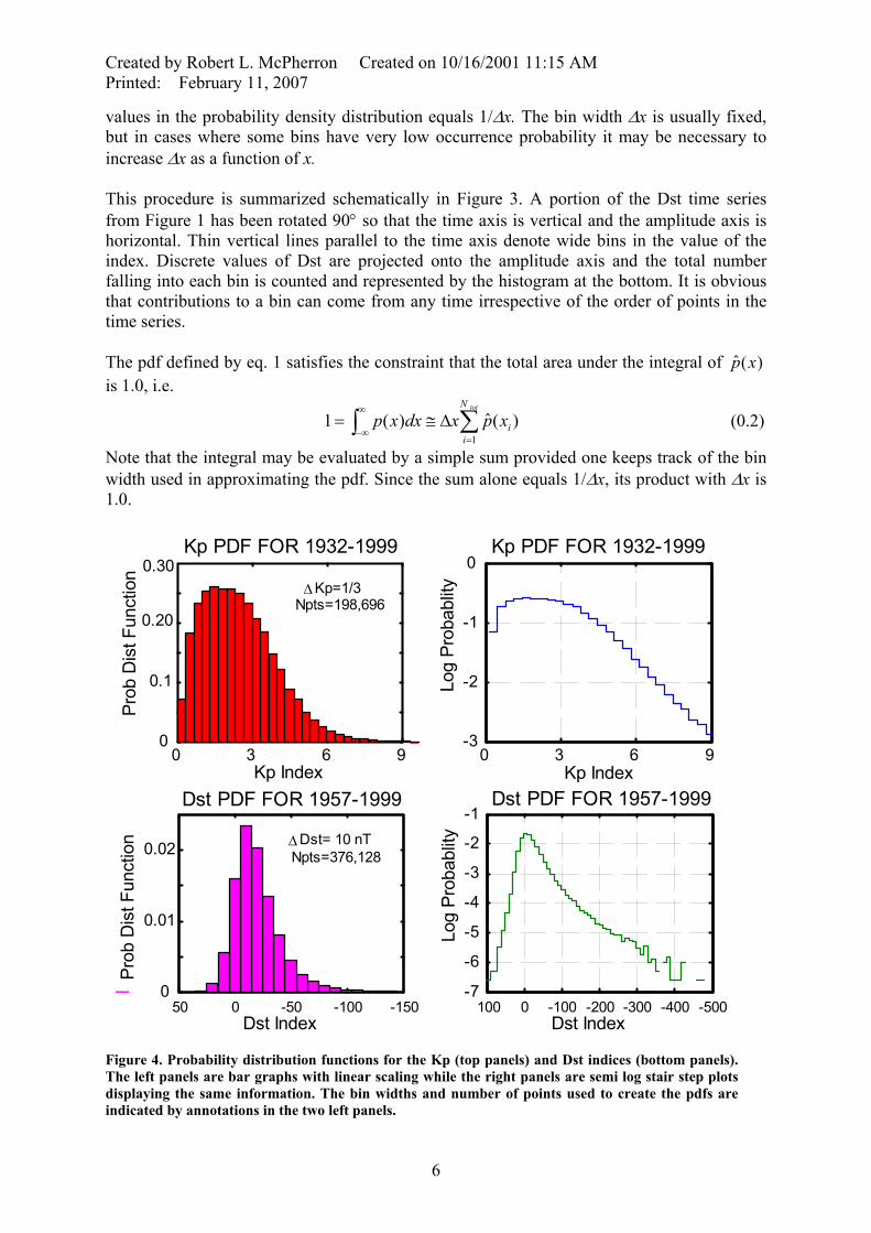
Figure 4. Probability distribution functions for the Kp (top panels) and Dst indices (bottom panels). The left panels are bar graphs with linear scaling while the right panels are semi log stair step plots displaying the same information. The bin widths and number of points used to create the pdfs are indicated by annotations in the two left panels.
6
Created by Robert L. McPherron Created on 10/16/2001 11:15 AM Printed: February 11, 2007
2.2.3.2 Estimation of the pdf Using Histograms A pdf can be created in a straightforward manner by sorting and counting. Sort all values in the set of observations into ascending order. Starting with the lowest bin edge, xi, count the number of values of x that are either equal to or greater than the left edge of the bin and less than the right edge, xi+1. This can also be done without sorting by calculating the bin number corresponding to the particular x and incrementing a count in the frequency distribution array at this location. The instruction indx = fix[(xi – x0)/∆x]+1 will calculate the proper location with x0 and ∆x defined as above. The pdfs for Kp and Dst indices are presented in Figure 4. The top left panel shows the pdf for Kp as a bar graph using a linear scale while the right panel shows the same information as a stair step semi log plot. Many geophysical parameters like Kp only rarely reach extreme values so that the probability of obtaining these values is very low. In such cases semi log plots more clearly reveal the range of variation in the pdf. The pdf for Kp was obtained by first dividing the archived values by 10 and then setting the edges of fixed width bins so that the quantized Kp values fall near the center of each bin, specifically x = [-1/6 : 1/3 : 9.1667]. (Note that the colon notation implies a series of values beginning at the leftmost number, increasing by the middle number, and ending at or before the rightmost number.) Because of their quantized nature the pdfs are plotted as bar graphs with the left edge of each bin corresponding to a possible value of the index. Kp is always positive and limited to 28 discrete values in the range [0, 9]. Dst can potentially have any value, however, the probability of both positive and negative extremes are so improbable that they have not yet occurred in the 43-year history of measurements of Dst. The bottom right panel shows a common problem encountered in estimating pdfs. Because extreme values of Dst are rare, the number of occurrences in a given bin is either zero or very small. Consequently estimates of extreme values of the pdf have large statistical errors corresponding to changes in the histogram by a single count. Missing bars in the graph correspond to bins with no occurrences. Not shown on the graph is one occurrence of a Dst = -589 nT. All intervening bins are empty. Other methods of estimating the pdf that compensate for this problem are discussed in Section 2.2.3.4. The graphs of the pdfs for both Kp and Dst demonstrate that these variables are not Gaussian, i.e. they do not have Gaussian shaped pdfs (see Section 2.2.3.4.4 below). By definition Kp has finite range and is skewed to positive values. Its pdf values is peaked around Kp ~ 2. Both high and low values of Kp have a low probability of occurrence. The pdf for Dst is skewed to extreme negative values (note that the x-axis for Dst has been reversed for comparison with the Kp distribution). Both large positive and negative values are rare. The most probable value of Dst is ~0. This property is a result of the definition of Dst that is designed to be approximately zero on the five quietest days of each month of the year.
2.2.3.3 Errors in the Simple Histogram To be completed….???????
2.2.3.4 Other Methods of Estimating the pdf In this section we use the Dst index to illustrate techniques for estimating probability distribution functions (pdf). These methods include the naive estimator, the nearest neighbor estimator, the kernel estimator, and the adaptive (variable) kernel method. We conclude with
7

Created by Robert L. McPherron Created on 10/16/2001 11:15 AM Printed: February 11, 2007
a comparison of pdf's determined by the different techniques. An extensive discussion of this topic is given by [Silverman, 1996 #2875].
2.2.3.4.1 The Naïve Estimator The standard histogram is not the best way to estimate a probability density function. At the extremes of the distribution some bins will be empty while others have only one or two occurrences. The calculated probability density will vary dramatically between adjacent bins due to fluctuations in the number of occurrences. This behavior was evident in the histogram for Dst discussed earlier. Increasing the bin width does not help because this tends to filter out important details in portions of the distribution where there is sufficient data for narrow bins. The histogram can also hide important details of the distribution through the particular choice of the locations of the bin edges. A better estimate of the pdf than the simple histogram is the naive estimator. Sorting the sequence of observations into ascending order, and then centering bins on every sample in the sorted distribution implements the simplest form of this estimator. The pdf is then estimated at any x by
[1ˆ ( ) ,2
p x Num x h x hh
]= − + (0.3)
Here the notation Num[] means the count of all values of xi that fall in the bin of width 2h centered at x. To avoid zeros the point x is chosen to be the locations of existing observations xi. This choice guarantees that every estimate will be finite and contain one or more samples. It also eliminates the problem of where to place the bin edges. The disadvantages of this scheme are that the bins are not equally spaced, and the bin widths are not optimized for either the tails, or the center of the distribution. The counting procedure may be represented mathematically by a weighted sum as follows. Define a weight function w(x) by
1 if abs(x) 12( )0 otherwise
w x⎧ <⎪= ⎨⎪⎩
(0.4)
Then the estimate at a fixed point x is given by
( )1
1 1ˆtotN
i
itot
x xp x wN h h=
−⎛= ⎜⎝ ⎠
∑ ⎞⎟ (0.5)
This formula is implemented by choosing a point x = xi and then counting all observations that lie in the interval ±h around this location, then dividing by the total number of observation Ntot, to obtain the probability, and finally dividing by the bin width 2h to obtain the probability density.
2.2.3.4.2 The Nearest Neighbor Estimator The difficulty with the naive pdf estimator discussed in Section 2.2.3.4.1 is the requirement that all bins are the same width regardless of the number of available observations. Clearly a better estimate could be obtained by requiring that the width of the bin be inversely proportional to the density of observations around a point. This estimate is called the nearest neighbor estimator. A way of accomplishing this is to define the bin so that it contains a fixed number of points, k. A typical choice is to use k = sqrt(Ntot). Then the bin edges are calculated in the following way. Let d(x,y) = |x-y| be the distance between any two points on the X axis. Let x be the point at which we are estimating the pdf. Then di(x) = |xi - x| is the distance between this point and the ith point on the line. Calculate all di(x) and sort them in
8
Created by Robert L. McPherron Created on 10/16/2001 11:15 AM Printed: February 11, 2007
ascending order. The first distance in this sequence is 0.0 corresponding to the point itself. Use all points in this sequence up to and including the kth point to estimate the pdf at point xi from the formula
( )ˆ2tot k
kp xN d
= (0.6)
This formula assumes the values used to calculate the estimate are symmetrically distributed about x for a distance dk on either side so that the bin width is 2dk. We may represent this estimate more formally by
( ) ( ) ( )1
1ˆtotN
i
itot k k
x xp x KN d x d x=
⎛ ⎞−= ⎜
⎝ ⎠∑ ⎟ (0.7)
The weight function (or kernel) K is again 1/2 for the symmetric range dk about the point x, and then zero beyond this distance. Note that the width of the kernel depends on the point x. The summation then gives the value k/2 reducing to the formula presented just above. The problem with the nearest neighbor estimate of the pdf near the extremes is the requirement that there be a fixed number of points in each estimate. Since there are no values of the variable beyond the extremes, the values used to make these estimates are not centered. For example, at the minimum of x all values contributing to the estimate come from points to the right of the extreme and hence are more probable. This elevates the estimate above its true value. In fact, it can be shown that the estimates at the left and right edges approach zero proportional to 1/x. The integral of such a distribution is infinite so clearly the nearest neighbor estimate is flawed at the extremes.
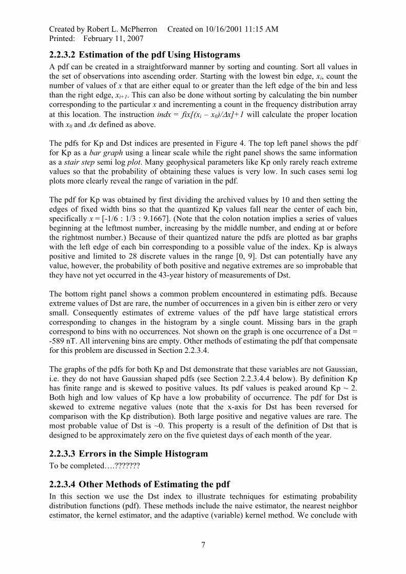
2.2.3.4.3 The Kernel Method The concept of making a weighted average of the samples of a distribution used in the naive estimator (see Section 2.2.3.4.1) can be generalized in the Kernel method [Silverman, 1996 #2875]. The basic idea is to center a symmetric probability distribution with unit area at each point in the distribution, then sum all the individual distributions, and divide by the total number of points. The idea is illustrated in Figure 5 taken from the book by Silverman. For this example the distribution consists of only seven points, and the kernel (or generalized weight function) is a Gaussian with unit area. The half width of the Gaussian is 0.2 units, a value narrow compared to the spread of the seven values shown by the symbol "X" along the x-axis. It is obvious that the width of the Gaussian is greater than the separation of the points so these elementary probability distributions overlap somewhat. Where they overlap they sum to a larger value than either distribution individually. The total pdf is shown by the sum of all of the elementary pdfs. For the choice of 0.2 as a smoothing parameter the final distribution is quite variable. The total pdf can be expressed mathematically as a discrete convolution of the Kernel with a distribution of delta functions centered at each point in the
Figure 5. An illustration of the use of fixed width kernels to estimate the pdf for a distribution of seven points on the x axis. Increasing the width of the kernel will smooth the pdf [Silverman, 1996 #2875].
9

Created by Robert L. McPherron Created on 10/16/2001 11:15 AM Printed: February 11, 2007
distribution. Let K(x) be a kernel function that satisfies the constraint that
(0.8) ( ) 1.0K x dx∞
−∞=∫
Then the estimate of the pdf is given by
( )1
1ˆtotN
i
itot
x xp x KN h h=
−⎛= ⎜⎝ ⎠
∑ ⎞⎟ (0.9)
This formula means that at any point x where we wish to estimate the total pdf, we must sum the contributions of all of the kernels centered on existing samples of the variable x. For quantized data the algorithm must be changed slightly centering the kernel only at each unique value in the distribution. But, the number of occurrences of this unique value then multiplies the kernel. Otherwise the calculation proceeds in the same way. The width to use for the smoothing kernel is difficult to determine. One approach is subjective. Simply try different values and choose one that corresponds to what you think is in the data. A more formal choice can be done mathematically, but unfortunately the result depends on the distribution being estimated. The basic idea is too minimize, over the entire distribution, the total mean square error of the estimate relative to the actual distribution. [Silverman, 1996 #2875] shows (page 40, equation 3.21) that the optimum half width h depends on the integral of the second derivative of the probability density. By considering a number of asymmetric distributions he shows that an optimum choice for h is given by
1 50.9
where min( , )opt Toth AN
A std iqr
−=
= (0.10)
Here std and iqr are statistical properties of the distribution of x calculated by the basic formulas given in Section 2.2.3.6. The primary advantage of the Kernel method using a fixed half width is that it can be easily implemented using the Fast Fourier Transform. Basically, one calculates the fft of both the sorted data and the kernel. These are multiplied and the product is inverse transformed to obtain the pdf. One important detail in this approach is to avoid errors due to circular convolution (See [Otnes, 1978 #927]). These occur because the fft function assumes that the underlying data are periodic with period equal to the length of the data sample, i.e. the total number of points. These errors can be eliminated by the use of zero padding. One simply loads the data into arrays that are twice as long as the original data array. These arrays are then handled as described above. Circular convolution occurs, but since the last half of each array is zero, no information is passed from the right edge of the arrays to the left in the transform process. After multiplying the transforms and inverse transforming one gets the correct result for the convolution.
2.2.3.4.4 The Variable Kernel Method A fixed-width kernel estimate of the pdf has the same problem as the naïve estimator; its width is a compromise that is neither optimum in the tails, nor the center of the distribution. A far better estimate can be obtained by adjusting the width of the kernel to the density of points as is done in the nearest neighbor method. However, instead of simply fixing the number of points used in an estimate as in the nearest neighbor method, the variable kernel method uses a pilot estimate of the pdf to define a scale for the kernel at each point. Also, it uses a kernel that is itself a probability density function with unit area. The sum of a finite number of such kernels, normalized by the total number, is therefore also a pdf with unit area. The formula used to calculate the pdf at any point x is then
10

Created by Robert L. McPherron Created on 10/16/2001 11:15 AM Printed: February 11, 2007
( )1
1 1ˆ TotNi
iTot i i
x xf x KN h hλ λ=
⎛ ⎞−= ⎜
⎝ ⎠∑ ⎟ (0.11)
Briefly the method works in the following way.
• Create a pilot pdf using one of the simpler methods described above • Create a pdf array on a grid of x spaced by ∆x between the extremes of x and initialize
all values to 0.0 • Start with the lowest unique value of xi and step sequentially through all unique
values • For each unique value xi calculate the number of occurrences of the value, N(xi). At
this point create a symmetric, non-negative, finite width kernel with area = 1.0, and a scale λ inversely proportional to the probability density at this point in the pilot pdf.
• Evaluate the kernel everywhere on the pdf grid • Multiply the kernel by N(xi) and add to the pdf array • Repeat for all unique values of the variable
The result obtained by applying this procedure to the Dst data is shown Figure 6. Vertical dashed lines show the extreme values of Dst found in the 43 years of available data. The heavy symmetric blue curves show the variable width kernels after multiplying by the number of occurrences of Dst at the center of each kernel. The black lines show the estimates of the pdf as the program loops through successively larger unique values of Dst. The red
-700 -600 -500 -400 -300 -200 -100 0 100 20010 -10
10 -9
10 -8
10 -7
10 -6
10 -5
10 -4
10 -3
10 -2
10 -1
10 0
Dst Inex (nT)
Pro
babi
lity
Den
sity
Fun
ctio
n
CREATION OF THE Dst PDF BY CONVOLUTION OF AN ADAPTIVE KERNEL
Min(Dst) Max(Dst)
AdaptiveKernel
Dst pdfSmoothed
∆Dst = 2h = 3
Figure 6. An example showing the creation of the probability density function for the Dst index using variable width kernels. The heavy blue lines are Epanechnikov kernels which are parabolas opening downward with finite normalized width of ±sqrt(5). Thin back lines show the cumulative sum of all kernels from the left side. The envelope shown by a heavy red line is the final sum and is the desired pdf.
11
Created by Robert L. McPherron Created on 10/16/2001 11:15 AM Printed: February 11, 2007
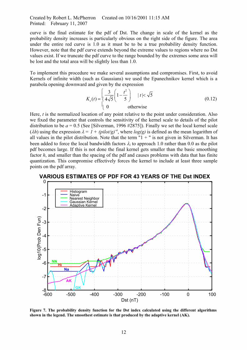
curve is the final estimate for the pdf of Dst. The change in scale of the kernel as the probability density increases is particularly obvious on the right side of the figure. The area under the entire red curve is 1.0 as it must be to be a true probability density function. However, note that the pdf curve extends beyond the extreme values to regions where no Dst values exist. If we truncate the pdf curve to the range bounded by the extremes some area will be lost and the total area will be slightly less than 1.0. To implement this procedure we make several assumptions and compromises. First, to avoid Kernels of infinite width (such as Gaussians) we used the Epanechnikov kernel which is a parabola opening downward and given by the expression
23 1 5( ) 54 5
0 otherwise e
t | t |K t
⎧ ⎛ ⎞− <⎪ ⎜ ⎟= ⎨ ⎝ ⎠
⎪⎩
(0.12)
Here, t is the normalized location of any point relative to the point under consideration. Also we fixed the parameter that controls the sensitivity of the kernel scale to details of the pilot distribution to be a = 0.5 (See [Silverman, 1996 #2875]). Finally we set the local kernel scale (λh) using the expression λ = 1 + (pilot/g)-a, where log(g) is defined as the mean logarithm of all values in the pilot distribution. Note that the term "1 + " is not given in Silverman. It has been added to force the local bandwidth factors λi to approach 1.0 rather than 0.0 as the pilot pdf becomes large. If this is not done the final kernel gets smaller than the basic smoothing factor h, and smaller than the spacing of the pdf and causes problems with data that has finite quantization. This compromise effectively forces the kernel to include at least three sample points on the pdf array.
-600 -500 -400 -300 -200 -100 0 100-8
-7
-6
-5
-4
-3
-2
-1
0
Dst (nT)
log1
0(P
rob
Den
Fun
)
VARIOUS ESTIMATES OF PDF FOR 43 YEARS OF THE Dst INDEX
HistogramNaiveNearest NeighborGaussian KernelAdaptive Kernel
HiNN
Na
GK
AK
Figure 7. The probability density function for the Dst index calculated using the different algorithms shown in the legend. The smoothest estimate is that produced by the adaptive kernel (AK).
12
Created by Robert L. McPherron Created on 10/16/2001 11:15 AM Printed: February 11, 2007
The probability density functions for the Dst index calculated by each of the various algorithms are compared in Figure 7. Only the adaptive techniques (nearest neighbors and variable kernel) create pdfs that are smooth in the tails of the distributions. The nearest neighbor estimate is clearly too large in the tails for the reasons discussed above. The adaptive (variable) kernel method produces a smooth curve that intuitively seems to agree well with the distribution of data points seen in the histogram.
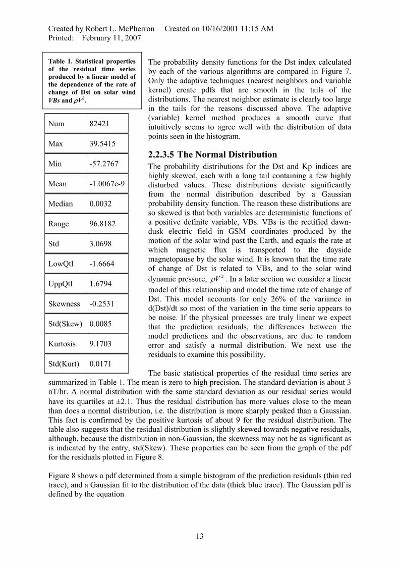
2.2.3.5 The Normal Distribution The probability distributions for the Dst and Kp indices are highly skewed, each with a long tail containing a few highly disturbed values. These distributions deviate significantly from the normal distribution described by a Gaussian probability density function. The reason these distributions are so skewed is that both variables are deterministic functions of a positive definite variable, VBs. VBs is the rectified dawn-dusk electric field in GSM coordinates produced by the motion of the solar wind past the Earth, and equals the rate at which magnetic flux is transported to the dayside magnetopause by the solar wind. It is known that the time rate of change of Dst is related to VBs, and to the solar wind dynamic pressure, 2Vρ . In a later section we consider a linear model of this relationship and model the time rate of change of Dst. This model accounts for only 26% of the variance in d(Dst)/dt so most of the variation in the time serie appears to be noise. If the physical processes are truly linear we expect that the prediction residuals, the differences between the model predictions and the observations, are due to random error and satisfy a normal distribution. We next use the residuals to examine this possibility. The basic statistical properties of the residual time series are
summarized in Table 1. The mean is zero to high precision. The standard deviation is about 3 nT/hr. A normal distribution with the same standard deviation as our residual series would have its quartiles at ±2.1. Thus the residual distribution has more values close to the mean than does a normal distribution, i.e. the distribution is more sharply peaked than a Gaussian. This fact is confirmed by the positive kurtosis of about 9 for the residual distribution. The table also suggests that the residual distribution is slightly skewed towards negative residuals, although, because the distribution in non-Gaussian, the skewness may not be as significant as is indicated by the entry, std(Skew). These properties can be seen from the graph of the pdf for the residuals plotted in Figure 8.
Table 1. Statistical properties of the residual time series produced by a linear model of the dependence of the rate of change of Dst on solar wind VBs and ρV2.
Num 82421
Max 39.5415
Min -57.2767
Mean -1.0067e-9
Median 0.0032
Range 96.8182
Std 3.0698
LowQtl -1.6664
UppQtl 1.6794
Skewness -0.2531
Std(Skew) 0.0085
Kurtosis 9.1703
Std(Kurt) 0.0171
Figure 8 shows a pdf determined from a simple histogram of the prediction residuals (thin red trace), and a Gaussian fit to the distribution of the data (thick blue trace). The Gaussian pdf is defined by the equation
13

Created by Robert L. McPherron Created on 10/16/2001 11:15 AM Printed: February 11, 2007
( )2
221( )2
x
f x eµ
σ
σ π
−−
= (0.13)
where x is the variable, µ is its mean value, and σ is its standard deviation. Note that the amplitude of this fit is constrained by the standard deviation so that the area underneath the pdf curve is 1.0.The fit is obtained by substituting the calculated mean and median for the residuals into this formula. If the histogram is examined in isolation the distribution appears to be Gaussian, However, when compared to the best-fit normal pdf it is obvious that the distribution is non-Gaussian. There are more values close to the mean than there are in the normal distribution. In compensation, there are too few values at intermediate values of the residual. Because of these differences, the amplitude of the fitted Gaussian pdf does not match the amplitude of the histogram. The semi log plot in the right panel reveals additional details of the residual pdf. Most obvious is the fact that there are too many values at large distances from the mean. Also, the left wing of the distribution is slightly higher than the right wing, confirming the negative skewness seen in Table 1. Since the residual distribution is non-Gaussian the confidence limits shown in the table for skewness and kurtosis are likely to be seriously in error since they are based on the assumption of a normal distribution.
2.2.3.6 Elementary Properties of the pdf
2.2.3.6.1 Extreme Values The extreme values of Kp are limited by definition to be 0.0 and 9.0. In the entire history of Kp used to create Figure 4 these extreme values were observed a number of times. However, because these values are quite rare, any small subset of the Kp values will not necessarily
-20 0 200
0.05
0.1
0.15
0.2
Residual (nT/hr)
Pro
babi
lity
Den
sity
PREDICTION RESIDUALS FOR HOURLY CHANGE IN Dst
-20 0 20
10 -4
10 -3
10 -2
10 -1
10 0
Residual (nT/hr)
Pro
babi
lity
Den
sity
Figure 8. A comparison of the pdf for model residuals (thin red line) with the best fit Gaussian pdf (thick blue line) to the same data. The pdf for the data clearly differs from the normal distribution by having too many values in the wings of the distribution.
14

Created by Robert L. McPherron Created on 10/16/2001 11:15 AM Printed: February 11, 2007
contain them. The number of points and extreme values in the Kp and Dst datasets are listed in the first three rows of Table 2.
2.2.3.6.2 Measures of Central Tendency Figure 4 shows that the Kp index tends to cluster around 2 and Dst clusters near zero. There are several common quantitative measures of this clustering tendency including the mean, median, and mode. The mean of a set of Ntot observations of a discrete variable xi is defined as
1
1 totN
iitot
x xN =
= ∑ (0.14)
The mean can also be calculated from the first moment of the pdf as follows
1 1
[ , ] 1( ) [ , ]tot totN N
i ii i
i itot tot
N x x xi ix xp x dx x x x N x x x
N x N
∞
= =−∞
+ ∆= ≅ ∆ = +
∆∑ ∑∫ ∆ (0.15)
If the width of successive bins is chosen such that no more than one x falls in each bin the formula reduces to the standard definition given above. For quantized data this is not possible as many observation have exactly the same value. In this case the sum may be broken into as many sub-sums as there are unique values of the variable. In each sub-sum xi is a constant for the sum and may be moved outside as a multiplier. The sub-sum then reduces to the count of the number of identical observations multiplied by the value. This is precisely the same result as obtained with the standard definition. The median of a probability distribution function p(x) is the value of xmed for which larger and smaller values are equally probable. Thus
1( ) ( )2
med
med
x
xp x dx p x dx
∞
−∞= =∫ ∫ (0.16)
For discrete values, sort the samples xi into ascending order and if Ntot is odd find the value of xi that has equal numbers of points above and below it. If it is even this is not possible so instead take the average of the two central values of the sorted distribution. If the samples have finite resolution and many samples are used to determine the median the two central values will often be the same and this makes no difference. The mode is defined as the value of xi corresponding to the maximum of the pdf. For a quantized variable like Kp this corresponds to the discrete value of Kp that occurs most frequently. More generally it is taken to be the value at the center of the bin containing the largest number of values. For continuous variables the definition depends on the width of bins used in determining the histogram. If the bins are too narrow there will be large fluctuations in the estimated pdf from bin to bin. If the bins are too large the location of the mode will be poorly resolved. It is not necessary to create a histogram to obtain the mode of a distribution [Press et al., 1986, page 462]. It can be calculated directly from the data in the following manner.
• Sort the data in ascending order. • Choose a window width of J samples (J >= 3). • For every i = 1, 2, …, Ntot–J estimate the pdf using the formula
[ ] ( )12 i i J
tot i J i
Jp x xN x x+
+
⎛ ⎞+ ≈⎜ ⎟ −⎝ ⎠ (0.17)
15

Created by Robert L. McPherron Created on 10/16/2001 11:15 AM Printed: February 11, 2007
• Take as the mode the value of [12 i i J ]x x ++ corresponding to the largest estimate of the
pdf. [Press et al., 1986] describes a complex procedure for choosing the most appropriate value of J.
These three measures of central tendency have been calculated for the Kp index using 68 years of data and for the Dst index using 43 years of data. The results are listed in rows 4-6 of Table 2. The total number of samples for both Kp (192,856) and Dst (376,128) is large so that the statistical properties have relatively small variance. For Kp the mode is smallest (1.333), the median is larger (2.000), while the mean is largest (2.323). Dst exhibits a similar pattern with mode (0 to –10), median (-12), and mean (-16.49). These values are closer to the minimum possible values of Kp and Dst than to the maximum indicating that geomagnetic activity is more often quiet than disturbed.
2.2.3.6.3 Measures of Dispersion It is obvious from the pdfs plotted in Figure 4 that the Kp and Dst values are spread around their central values. Three standard measures of this dispersion include the mean absolute deviation, the standard deviation, and the interquartile range. The average absolute deviation is defined by the formula mean(abs( ))imad x x= − (0.18) The standard deviation (root mean square) is given by
( )2
1
11
totN
iitot
std x xN =
=− ∑ −
1
(0.19)
The upper and lower quartiles are defined in the same way as the median (eq. 5) except that the values ¼ and ¾ are used instead of ½. The interquartile range (iqr) is the difference between the upper and lower quartiles (Q3 and Q1) 3iqr Q Q= − (0.20) For variables with a Gaussian pdf 67% of all data values will lie within ±1 std of the mean. Similary, by definition 50% of the data values fall within the interquartile range. Note that the standard deviation is more sensitive to values far from the mean than is the average absolute deviation. The values of these measures of dispersion for the Kp and Dst indices are also shown in Table 2. For both indices the separations of the upper and lower quartiles from the corresponding median are unequal. This property is a consequence of the asymmetric nature of their pdfs. A measure of this asymmetry is discussed next.
2.2.3.6.4 Measures of Asymmetry The standard measure of asymmetry of a pdf is called skewness. It is defined by the third moment of the probability distribution
( )3x xSkewness p x dx
σ
∞
−∞
−⎛ ⎞= ⎜ ⎟⎝ ⎠∫ (0.21)
Because of the standard deviation in the denominator, skewness is a dimensionless quantity. For sampled data this definition reduces to the formula
3
1
1 totN
itot
x xskewnessN σ=
−⎛= ⎜⎝ ⎠
∑ ⎞⎟ (0.22)
16
Created by Robert L. McPherron Created on 10/16/2001 11:15 AM Printed: February 11, 2007
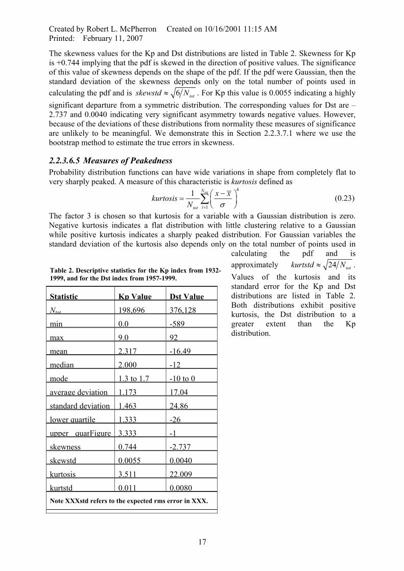
The skewness values for the Kp and Dst distributions are listed in Table 2. Skewness for Kp is +0.744 implying that the pdf is skewed in the direction of positive values. The significance of this value of skewness depends on the shape of the pdf. If the pdf were Gaussian, then the standard deviation of the skewness depends only on the total number of points used in calculating the pdf and is 6 totskewstd N≈ . For Kp this value is 0.0055 indicating a highly significant departure from a symmetric distribution. The corresponding values for Dst are –2.737 and 0.0040 indicating very significant asymmetry towards negative values. However, because of the deviations of these distributions from normality these measures of significance are unlikely to be meaningful. We demonstrate this in Section 2.2.3.7.1 where we use the bootstrap method to estimate the true errors in skewness.
2.2.3.6.5 Measures of Peakedness Probability distribution functions can have wide variations in shape from completely flat to very sharply peaked. A measure of this characteristic is kurtosis defined as
4
1
1 totN
itot
x xkurtosisN σ=
−⎛= ⎜⎝ ⎠
∑ ⎞⎟ (0.23)
The factor 3 is chosen so that kurtosis for a variable with a Gaussian distribution is zero. Negative kurtosis indicates a flat distribution with little clustering relative to a Gaussian while positive kurtosis indicates a sharply peaked distribution. For Gaussian variables the standard deviation of the kurtosis also depends only on the total number of points used in
calculating the pdf and is approximately 24kurtstd N≈ tot . Values of the kurtosis and its standard error for the Kp and Dst distributions are listed in Table 2. Both distributions exhibit positive kurtosis, the Dst distribution to a greater extent than the Kp distribution.
Table 2. Descriptive statistics for the Kp index from 1932-1999, and for the Dst index from 1957-1999.
Statistic Kp Value Dst Value
Ntot 198,696 376,128
min 0.0 -589
max 9.0 92
mean 2.317 -16.49
median 2.000 -12
mode 1.3 to 1.7 -10 to 0
average deviation 1.173 17.04
standard deviation 1.463 24.86
lower quartile 1.333 -26
upper quarFigure 3.333 -1
skewness 0.744 -2.737
skewstd 0.0055 0.0040
kurtosis 3.511 22.009
kurtstd 0.011 0.0080Note XXXstd refers to the expected rms error in XXX.
17
Created by Robert L. McPherron Created on 10/16/2001 11:15 AM Printed: February 11, 2007
2.2.3.7 Description of the Bootstrap Method For many of the statistical procedures used in this book it is difficult to determine the size of the errors in quantities calculated from data. In some cases this is because of the complexity of the underlying algorithms. Often, however, it is because the error calculations can only be done for data that are normally distributed. As we saw earlier, most physical variables do not satisfy such distributions. In such cases one can resort to more empirical methods to determine the errors. The simplest such method is to repeat the experiment a number of times producing an ensemble of datasets that are subjected to identical analysis. If this is done enough times one can determine a pdf for the calculated quantity and from this determine the rms deviation in its value. Unfortunately, much of the time we have only one dataset produced by nature and are unable to repeat the experiment to obtain multiple realizations of the signal. In such cases we can resort to simulation to calculate the errors. A sophisticated way of doing this is to produce many new time series with the same statistical properties as the dataset being studied. For example, if temporal order is unimportant then all one needs to do is to produce a sequence of random numbers that has the same pdf as the measured data. Many such simulated datasets created in this way can then be analyzed by the same procedure and the error determined from the pdf of the results. If not enough is known about the statistical properties of the variables involved then a crude error estimate can be obtained by the bootstrap method. In this technique the measured data themselves are used to create new datasets that are subsequently analyzed. In the bootstrap method a uniform distribution is used to sample the original dataset of N data points. Samples are selected from the original and copied to the simulated dataset until it contains the same number of points as the original. Since no samples are removed from the original a particular sample may be copied several times at the expense of other samples. In this way each simulated dataset contains slightly different collections of measured data points. Analysis of each of these datasets then produces a distribution of calculated values that can be characterized by a mean and standard deviation.
2.2.3.7.1 Estimation of the Errors in Elementary Properties We illustrate the bootstrap procedure using the distribution of residuals discussed in Section 2.2.3.5. As shown in this section the pdf of the residuals is not Gaussian hence the estimates of errors in higher moments of the pdf such as kurtosis are dubious. Therefore we have used the bootstrap method to produce 100 different simulations of the original data. For each simulation we calculate the kurtosis, and then from the set of simulations produce a mean and standard deviation of the kurtosis. The text in the upper left corner of the figure shows the bootstrap results with a kurtosis of 9.1870 and a standard deviation of 1.5 for the ensemble of simulations. In comparison, the text in the upper right shows the values calculated for the original data under the assumption that the residual distribution is Gaussian. Although the mean kurtosis from the ensemble is nearly identical to the kurtosis of the original data, the error calculated from the ensemble is much larger than expected for a Gaussian distribution. Note, however, the kurtosis is positive and much larger than its estimated error so that the implication of Table 1 that the distribution is more sharply peaked than a Gaussian still stands.
2.2.3.7.2 Estimation of the Errors in a pdf ?????????????????
18

Created by Robert L. McPherron Created on 10/16/2001 11:15 AM Printed: February 11, 2007
5 10 150
5
10
15
20
25
30
Kurtosis of Residual
Num
ber o
f Occ
urre
nces
Bootstrap Determination of Kurtosis
BootStrap Statistics Num: 100 <Kurtosis>: 9.1870 Var(Kurtosis): 1.5068
Normal Fit Statistics Num: 82421 Kurtosis: 9.1703 Var(Kur): 0.0171
Figure 9. A histogram of kurtosis values calculated from a bootstrap simulation with 100 time series derived from the residual time series discussed in Section 2.2.3.5. The mean and standard deviation derived from this pdf are shown in the upper left. For comparison the same values calculated under the assumption the residual distribution is Gaussian are shown in the upper right.
2.2.4 Cumulative Distribution Function (cdf)
2.2.4.1 Definition of the cdf The cumulative distribution function or cdf is defined as the integral of the pdf. Thus
( ) ( )x
cdf x p x dx−∞
′ ′= ∫ (0.24)
Approximate the integral by a sum using the same ∆x used in calculating the pdf so that
(0.25) 1
( ) ( )n
ni
cdf x x p x=
= ∆ ∑ i
where xn denotes the left edge of the (n+1)th bin and the sum is over all bins including this bin. Substitute the definition of the pdf (eq. ) obtaining
0 0
[ , ] 1( ) [ , ]n n
i in
i itot tot
N x x xcdf x x N x x xN x N= =
+ ∆= ∆ = + ∆
∆∑ ∑ i i (0.26)
The sum represents the total number of occurrences of values of x less than the right edge of the nth bin.
19
Created by Robert L. McPherron Created on 10/16/2001 11:15 AM Printed: February 11, 2007
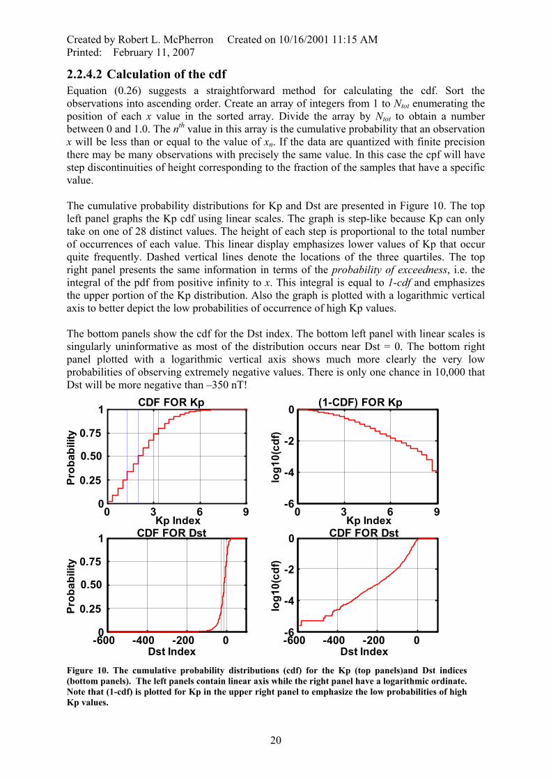
2.2.4.2 Calculation of the cdf Equation (0.26) suggests a straightforward method for calculating the cdf. Sort the observations into ascending order. Create an array of integers from 1 to Ntot enumerating the position of each x value in the sorted array. Divide the array by Ntot to obtain a number between 0 and 1.0. The nth value in this array is the cumulative probability that an observation x will be less than or equal to the value of xn. If the data are quantized with finite precision there may be many observations with precisely the same value. In this case the cpf will have step discontinuities of height corresponding to the fraction of the samples that have a specific value. The cumulative probability distributions for Kp and Dst are presented in Figure 10. The top left panel graphs the Kp cdf using linear scales. The graph is step-like because Kp can only take on one of 28 distinct values. The height of each step is proportional to the total number of occurrences of each value. This linear display emphasizes lower values of Kp that occur quite frequently. Dashed vertical lines denote the locations of the three quartiles. The top right panel presents the same information in terms of the probability of exceedness, i.e. the integral of the pdf from positive infinity to x. This integral is equal to 1-cdf and emphasizes the upper portion of the Kp distribution. Also the graph is plotted with a logarithmic vertical axis to better depict the low probabilities of occurrence of high Kp values. The bottom panels show the cdf for the Dst index. The bottom left panel with linear scales is singularly uninformative as most of the distribution occurs near Dst = 0. The bottom right panel plotted with a logarithmic vertical axis shows much more clearly the very low probabilities of observing extremely negative values. There is only one chance in 10,000 that Dst will be more negative than –350 nT!
0 3 6 90
0.25
0.50
0.75
1
Kp Index
Prob
abili
ty
CDF FOR Kp
0 3 6 9-6
-4
-2
0
Kp Index
log1
0(cd
f)
(1-CDF) FOR Kp
-600 -400 -200 00
0.25
0.50
0.75
1
Dst Index
Prob
abili
ty
CDF FOR Dst
-600 -400 -200 0-6
-4
-2
0
Dst Index
log1
0(cd
f)
CDF FOR Dst
Figure 10. The cumulative probability distributions (cdf) for the Kp (top panels)and Dst indices (bottom panels). The left panels contain linear axis while the right panel have a logarithmic ordinate. Note that (1-cdf) is plotted for Kp in the upper right panel to emphasize the low probabilities of high Kp values.
20
Created by Robert L. McPherron Created on 10/16/2001 11:15 AM Printed: February 11, 2007
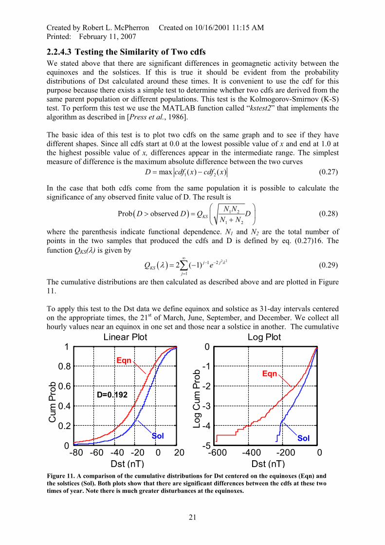
2.2.4.3 Testing the Similarity of Two cdfs We stated above that there are significant differences in geomagnetic activity between the equinoxes and the solstices. If this is true it should be evident from the probability distributions of Dst calculated around these times. It is convenient to use the cdf for this purpose because there exists a simple test to determine whether two cdfs are derived from the same parent population or different populations. This test is the Kolmogorov-Smirnov (K-S) test. To perform this test we use the MATLAB function called “kstest2” that implements the algorithm as described in [Press et al., 1986]. The basic idea of this test is to plot two cdfs on the same graph and to see if they have different shapes. Since all cdfs start at 0.0 at the lowest possible value of x and end at 1.0 at the highest possible value of x, differences appear in the intermediate range. The simplest measure of difference is the maximum absolute difference between the two curves 1 2max ( ) ( )D cdf x cdf x= − (0.27)
In the case that both cdfs come from the same population it is possible to calculate the significance of any observed finite value of D. The result is
( ) 1 2
1 2
Prob observed KSN ND D Q
N N⎛ ⎞
> = ⎜ +⎝ ⎠D ⎟
e
(0.28)
where the parenthesis indicate functional dependence. N1 and N2 are the total number of points in the two samples that produced the cdfs and D is defined by eq. (0.27)16. The function QKS(λ) is given by
( ) 2 21 2
1
2 ( 1) j jKS
j
Q λλ∞
− −
=
= −∑ (0.29)
The cumulative distributions are then calculated as described above and are plotted in Figure 11. To apply this test to the Dst data we define equinox and solstice as 31-day intervals centered on the appropriate times, the 21st of March, June, September, and December. We collect all hourly values near an equinox in one set and those near a solstice in another. The cumulative
-80 -60 -40 -20 0 200
0.2
0.4
0.6
0.8
1
Dst (nT)
Cum
Pro
b
Eqn
Sol
D=0.192
Linear Plot
-600 -400 -200 0-5
-4
-3
-2
-1
0
Dst (nT)
Log
Cum
Pro
b
Log Plot
Eqn
Sol
Figure 11. A comparison of the cumulative distributions for Dst centered on the equinoxes (Eqn) and the solstices (Sol). Both plots show that there are significant differences between the cdfs at these two times of year. Note there is much greater disturbances at the equinoxes.
21

Created by Robert L. McPherron Created on 10/16/2001 11:15 AM Printed: February 11, 2007
distributions are then calculated as described above and are plotted in Figure 11. Both panels of Figure 11 show that there is a significant difference between the two cdfs.
2.2.4.4 Testing a cdf for Normality df is close to being a Gaussian is with a quantile-
he figure shows immediately that the distribution of residuals departs significantly from a
From the log plot in the right panel it is evident that Dst was never less than –250 nT at the solstice, but it reaches nearly –600 nT at the equinox. The left panel shows the application of the Kolmogorov-Smirnov test to the two cdfs. The maximum difference between the two curves is D = 19.2% at a Dst value of about ????. From the facts that the step size of the curves is much smaller than their separation, and that the two curves never intersect, it would seem likely that these represent cdfs from two different source populations. Applying the K-S test we find that the probability that D would exceed the observed value of ~20% is 0.0! The MATLAB function finds this probability less than the smallest possible double precision value for the exponential, i.e. prob < 10-746. There is no possibility that the same parent population could produce these two distributions by chance.
One way of determining whether a sample pquantile plot (qqplot). This plot is obtained by constructing the cumulative distribution functions (cd) for both the variable of interest, and a second variable with the same number of samples, but which satisfies a normal distribution with zero mean and unit standard deviation. One then constructs a graph using the quantiles of the normal distribution as abscissa, and the quantiles of the sample distribution as the ordinate. If the graph is a straight line the sample distribution is Gaussian. Departures from a line indicate a non-Gaussian distribution. A quantile plot for our distribution is plotted in Figure 12. T
-5 -4 -3 -2 -1 0 1 2 3 4 5-40
-30
-20
-10
0
10
20
30
40
Location in Normal Dist (std)
Val
ue o
f Res
idua
l
QQ PLOT OF RESIDUAL VERSUS STANDARD NORMAL
Quartile Line
Normal Relation
Observed Relation
Figure 12. A quantile-quantile plot for the Dst model residuals. The cdf of the sample distribution is plotted as the ordinate and the cdf of a normal distribution with the same number of points as the sample is plotted as the abscissa. The long line shows the expected relation if the sample distribution is normal. The short thick red line connects the quartiles of the two distributions. Crosses show the actual relation between the sample and normal distributions.
22
Created by Robert L. McPherron Created on 10/16/2001 11:15 AM Printed: February 11, 2007
normal distribution, and that the discrepancy is in both wings of the distribution. In Figure 12 the blue crosses depict the actual relation between the residual distribution and a normal distribution. Similarly, the long green line portrays the relation expected if the residual distribution were Gaussian. The short, thick red line connects the quartiles of the two distributions. It is apparent that the residual distribution is approximately normal for ±1.5 standard deviations on either side of the median (remember that the std for the residual distribution was ~3).
2.2.5 The Joint Probability Distribution sed to establish whether two variables x
.
is
he jpdf is defined by analogy with the pdf of a single variable
The joint probability density distribution (jpdf) is uand y are related. Assume that both variables are sampled simultaneously a total of Ntot timesThe sample pairs (tuples) may be recorded in a table with two columns and Ntot rows. This table is often called a flat file because it will lay flat on a desktop. Flat files are particularly easy to read and write because they consist of a single record type repeated for each row. Thflat file is also called a relation since the entire table contains information about how one variable is related to the other. The joint probability distribution is a visualization of this relation. T
0 0
;j j i iN[x ,x ∆x y , y+ +( , ) lim limxy j i x y
tot
∆y]p x y
N ∆x∆y∆ → ∆ →
⎛ ⎞⎜ ⎟⎝ ⎠
(0.30)
The subscript notation (xj, yi) emphasizes the fact that in graphs the x-axis is generally taken
the
o illustrate the calculation of a jpdf and the information that may be derived from it we st
=
to be horizontal and the y-axis as vertical, but in a table the horizontal direction corresponds to columns that are commonly denoted in matrix notation by the second index j. The quantityN[.] is the total number of occurrences of tuples in the relation that lie within the left- and bottom-bounded bin defined by the values within the parentheses. Division by Ntot convertsthis number to the probability that a tuple from the particular relation defined by the Ntot samples, falls in this bin. Finally, division by the product of the widths of the bin convertsprobability to a probability density. Again the sum of the probabilities in all bins is 1.0, and the integral (product of widths times double sum) of the probability density is also 1.0. Tconsider the Dst index. Many years ago [Burton, 1975 #226] showed that the corrected Dindex ( *
stD ) satisfies the differential equation
( ) ( )* *st stD
a VBsdt
d D
τ= ∗ − (0.31)
VBs is the rectified solar wind electric field which is zero when the z comHere ponent of the interplanetary magnetic field is northward, τ is the rate at which *
stD recovers when VBs is zero, and α is a low pass filter convolved with VBs. As shown by these authors, corrected
*stD is related to the measured Dst index by the relation
*D D b p cst st dyn= + − (0.32)
here pdyn is the solar wind dynamic pressure, b w = 8.555 nT/ nP is a constant of proportionality, and c is a correction related to baselines of the mag grams from which Dst is calculated. If we correct the observed Dst index for solar wind dynamic pressure we obtain a new variable,
neto
*st dyn stx D b p D c= − = − . Then the differential equation can be
rewritten in terms of x as
23

Created by Robert L. McPherron Created on 10/16/2001 11:15 AM Printed: February 11, 2007
dx x cVBsdt
ατ τ
= ∗ −
plies that the rate of change of x is linearly proportional to x. To emonstrate the validity of this equation we utilize the e
is s
− (0.33)
If VBs is zero, eq. (0.33) imd ntire history of solar wind measurements from 1963 to 2000 to create a joint distribution between dx/dt and x. This distribution is presented in the upper left panel of Figure 13. It can be seen that dx/dtelated to x, decreasing as x increases. However, it is obvious that the noise in dx/dt ir
comparable to, or larger, than the systematic variation. Below in section ??? we define the linear correlation coefficient between two variables. A value of 0.0 means no correlation while 1.0 means perfect correlation. For the data shown in Figure 13 the correlation coefficient is only 0.36, but as we show later, still very significant. We can parameterize therelation shown in the joint distribution by performing a linear regression of dx/dt against x
as
discussed in Section????. The results are shown below the histogram. The baseline correctionc is very small, 1.9 nT, but the decay constant τ = 17.2 hours is long compared to the estimateobtained by [Burton, 1975 #226]. An explanation for this difference has been given recently by [O'Brien, 2000 #2874].
2.2.5.1 Estimation with 2-D histograms The joint distribution shown in Figure 13
was calculated using the two-dimensional ters of this histogram are summarized in
the Dst histogram technique described above. The paramethe bottom right panel. Ntot = 317,016 is the total number of hourly measurements of index since the beginning of the space age. Nder = 184,101 is the total number of corrected
-200 -150 -100 -50 0 50-20
-10
0
10
20
d(cD
st)/d
t (nT
/hr)
-6-5 -4 -3
d(cDst)/dt = -(cDst+1.9)/17.19
-200 -150 -100 -50 0 5010 -5
10 -3
10 -1
cDst (nT)
10 -4 10 -2 10 0-20
-10
0
10
20
pdfNtot =317,016Nder = 184,101NBn=86,315Ngood =61,373Nout =60
Dst=25d(Dst)/dt)=2
∆∆
Figure 13. The joint probability distribution for the rate of change of pressure corrected Dst and corrected Dst is plotted as a contour map in the upper left panel. The bottom left panel shows the marginal distribution for corrected Dst obtained by integrating vertically over all rates of change. The upper right panel is the marginal distribution for the rate of change. The bottom right panel shows the number of data points used to create the distribution (see text).
24
Created by Robert L. McPherron Created on 10/16/2001 11:15 AM Printed: February 11, 2007
time derivatives of Dst available during this time interval. This number is about half the total because the spacecraft used to monitor the solar wind is often inside the Earth’s magnetosphere and hence unable to monitor the solar wind. NBn = 86,315 is the total number of times that solar wind magnetic field were available, and that the field was nortN
hward.
ct
arly
mbers vividly illustrate one of the main problems of multivariant analysis of ace physics data. The product of several independent probabilities is usually a small
e , 2000
Distributions Figure 13 are called marginal
g the joint probability density distribution over
, ,
M
x j xy xy j ii
p x p x y dy y p x y
−∞
∞
=−∞
= = ∆ ∑∫ (0.34)
Because the bins must be fairly large to estimate the joint probability density function, the pdfs obtained in this way for the two variables are quite coarse. Both pdfs satisfy the
lity observing a particular value of one variable
ther. It is represented by the notation h(y|x) [or
l
good = 61,373 is the number of simultaneous corrected derivatives, and northward solar windfield. This number, only about 1/5 of the total number of data points, was used to construthe joint distribution. The size of the bins is shown by the rectangle in the histogram, and corresponds to 25 nT by 2 nT/hr. Note that in the entire history of space physics only 60 values fall outside the limits of this histogram, even though Dst = -200 nT is not a particulgreat storm. The above nuspnumber. When a calculation depends on several variables, all must be available to perform the calculation. The problem becomes particularly acute when one tries to estimate the various parameters in the Dst equation for the extreme values of VBs that generate very negative values of Dst. Extreme values are extremely rare, yet we want to know if the differential equation remains the same as it is for VBs = 0, and whether the parameters arconstant as assumed by [Burton, 1975 #72]. Recently [McPherron, 2001 #294; O'Brien#287] showed that all of the parameters depend nonlinearly on VBs, but the form of the equation does not change.
2.2.5.2 The Marginal The histograms shown at the bottom left and upper right of distributions. They are obtained by integratineach variable separately. For example, integrating horizontally over corrected Dst gives theprobability density function for the rate of change of corrected Dst. Since the joint distribution is known only at discrete points the integrals can be replaced by a sum so that
( ) ( ) ( ), ,N
y i xy xy j ij
p y p x y dx x p x y∞
=
= = ∆ ∑∫
( ) ( ) ( )1
1
requirement that their integrals are 1.0.
2.2.5.3 The Conditional ProbabiThe conditional probability is the probability ofgiven that we already know the value of the oby h(x|y)] which is read as the probability density for observing some value of y given that we already know the value of x. But the joint probability density function for a given x defines the relative probability for different values of y. Thus all that is needed is to assure that the total integral is 1.0. This is achieved by normalizing the joint pdf by the marginadistribution. Thus
( , )
( | ) j
( )jx j
p x yh y x
p xIf we integrate h(y|xj) over all y we have
=
25
Created by Robert L. McPherron Created on 10/16/2001 11:15 AM Printed: February 11, 2007
( ) ( )1
1
1 1
( , )( , ) ( , )( | ) 1.0
( )jx jp x−∞ −∞
⎜ ⎟⎝ ⎠
∫ ∫, ,
M
xy j iMxy j xy j i i
M Mi
xy j l xy j ll l
p x yp x y p x yh y x dy dy y
y p x y p x y
∞ ∞=
=
= =
⎛ ⎞= = ∆ = =⎜ ⎟
∆
∑∑
∑ ∑ (0.35)
laced the marginal distribution in the denominator by its efinition and noted that the ratio of the two sums is 1.0.
In the preceding integral we have repd
2.2.6 Correlation Coefficient The variance of a single variable is defined as the mean square variation of a quantity about its mean value. Thus
( )2 11xx i
iTot
1 TotN
x x−∑ (0.36)
0.19) shows that it is the square of the standard deviation. The covariance between two variables x and y is defined in a similar manner as
N =−Comparison with eq. (
σ =
( )( )11xy i i
iTot
1 TotN
x x y yσ = − −∑ (0.37)
y about zero. Thus each is sometimes positive and sometimes negative. If the two differences change
gether then they will both be positive or negative at the samer. r is
ange
N =−Since the means have been subtracted from each variable the differences var
to e point. Their product will therefore be positive, and the sum of many positive products will be a large positive numbAlternatively they may vary in precisely the opposite way so when one is positive the othenegative. The sum will then be a large negative number. If instead the two differences chin a random way with respect to each other there will be approximately equal numbers of positive and negative terms and the sum will be a small number. The variance is a special case of the covariance where y is replaced by x. Since the two series are identical the differences from the mean change in exactly the same way and the variance is a large positive number. The correlation coefficient ρxy is defined as the covariance normalized by the product of the standard deviations of both series. Thus
11xy
iTotxx yy xx yy
1 TotNxy i ix x y yσ ⎛ ⎞⎛ ⎞− −
Nρ
σ σ σ σ=
⎜ ⎟= = ⎜ ⎟⎜ ⎟⎜ ⎟− ⎝ ⎠⎝ ⎠nless number since the denominators of each factor
ave the same units as the numerators. In addition, its maximum ame replace one series by the other and the sum reduces to the varia
pendence of dx/dt on x
∑ (0.38)
The correlation coefficient is a dimensioh plitude is obtained when w nce of the series. But the product of the terms in the denominator also gives the variance so the ratio reduces to 1.0. Similarly if we replace one series by the negative of the other we have perfect anticorrelation of the two variables and the expression reduces to –1.0. Thus the correlation coefficient varies between –1 and 1. A value of 0.0 implies no correlation at all. To illustrate the application of this formula we apply it to the data used to generate the joint probability density function plotted in Figure 13. The result is ρxy = 0.3673. This is a relatively low number, but obviously consistent with the obvious decombined with the distribution of values around the linear fit to the data. The expected error in this number is hard to estimate as it depends on the pdfs for the two variables. However, when the number of points is large the distribution function describing the correlation
26
Created by Robert L. McPherron Created on 10/16/2001 11:15 AM Printed: February 11, 2007
coefficient is roughly Gaussian with a standard deviation of 1/ TotN [Press, 1986 #2296]. In our case this error is 4.04 x 10⁻³, i.e. the correlation coefficient should be significant to the third decimal point. If we postulate that this number is simply a chance fluctuation from zero we find that the probability of this happening is absolutely zero to the accuracy of the calculation. When we use the bootstrap method to estimate the correlation coefficient and its error we find for an ensemble of 100 simulated datasets that ρxy = 0.3674 ± 0.0064. These values are quiet close to those quoted above.
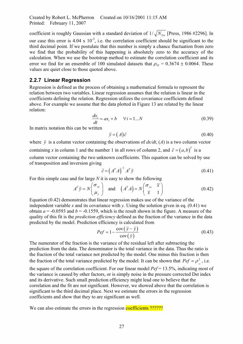
2.2.7 Linear Regression Regression is defined as the process of obtaining a mathematical formula to represent the
near regression assumes that the relation is linear in the Regression utilizes the covariance coefficients defined
relation between two variables. Licoefficients defining the relation.above. For example we assume that the data plotted in Figure 13 are related by the linear relation:
1...ii
dx ax b i Ndt
= + ∀ = (0.
In matrix
39)
notation this can be written ( )y A= cr r (0.40)
g the observations of dx/dt, (A) is a two column vector
ontaining x in column 1 and the number 1 in all r v
where y is a column vector containinr
c ows of column 2, and ( ), Tc a b=r is a
column ector containing the two unknown coefficients. This equation can be solved by use of transposition and inversion giving ( ) 1
ˆ T Tc A A A y−
=r (0.41)
For this simple case and for large N it is easy to show the following
( ) and xyT T 1y
xx xA y N A A
σ⎛ ⎞= ⎜ ⎟
r
dependent variable x and its covariance with y. Using the solutionobtain a = -0.0593 and b = -0.1559, which is the result shown in the figure. A measure of the
the data
Nσ⎛ ⎞
= ⎜ ⎟ (0.42) xµ ⎝ ⎠⎝ ⎠
Equation (0.42) demonstrates that linear regression makes use of the variance of the in given in eq. (0.41) we
quality of this fit is the prediction efficiency defined as the fraction of the variance in predicted by the model. Prediction efficiency is calculated from
( )( )
ˆcov1
covy y
Pefy−
= −r
r (0.43)
The numerator of the fraction is the variance of the residual left after subtracting the p ariance in the data. Thus the ratio is rediction from the data. The denominator is the total vthe fraction of the total variance not predicted by the model. One minus this fraction is then the fraction of the total variance predicted by the model. It can be shown that
xyPef 2ρ=
the square of the correlation coefficient. For our linear model Pef = 13.5%, indicating most othe variance is caused by other factors, or is simply noise in the pressure corrected Dst index and its derivative. Such small prediction efficiency might lead one to believe tcorrelation and the fit are not significant. However, we showed above that the correlation is significant to the third decimal place. Next we estimate the errors in the regression coefficients and show that they to are significant as well.
, i.e. f
hat the
We can also estimate the errors in the regression coefficients ??????
27
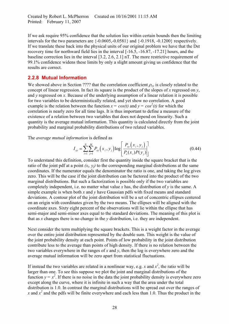
Created by Robert L. McPherron Created on 10/16/2001 11:15 AM Printed: February 11, 2007
If we ask require 95% confidence that the solution lies within certain bounds then the limiting
tervals for the two parameters are {-0.0605,-0.0581} and {-0.1918, -0.1200} respectively. m we have that the Dst
covery time for northward field lies in the interval [-16.5, -16.87, -17.21] hours, and the
ression. In fact its square is the product of the slopes of x regressed on y, ing assumption of a linear relation it is possible
ically related, and yet show no correlation. A good
e joint
inIf we translate these back into the physical units of our original problerebaseline correction lies in the interval [3.2, 2.6, 2.1] nT. The more restrictive requirement of 99.1% confidence widens these limits by only a slight amount giving us confidence that the results are correct.
2.2.8 Mutual Information We showed above in Section ???? that the correlation coefficient ρxy is closely related to the concept of linear regand y regressed on x. Because of the underlyfor two variables to be deterministexample is the relation between the function x = cos(t) and y = cos2(t) for which the correlation is nearly zero for all time lags. It is thus important to define a measure of the existence of a relation between two variables that does not depend on linearity. Such a quantity is the average mutual information. This quantity is calculated directly from thprobability and marginal probability distributions of two related variables. The average mutual information is defined as
( ) ( )1 1
,, log
( ) ( )
N Mxy i j
xy xy i j
P x yI P x y
P x P yi j x i j= =
⎡ ⎤= ⎢ ⎥
⎢ ⎥⎣ ⎦(0.44)
quantity inside the square bracket that is the ratio of the joint pdf at a point (xi, yj) to the corresponding marginal distributions at the same oordinates. If the numerator equals the denominator the ratio is o
zero. This will be the case if the joint distribution can be factored into the product of the two
the
ot is
ge
ibution ontribute less to the average than points of high density. If there is no relation between the
everywhere zero xcept along the curve, where it is infinite in such a way that the area under the total
s of in the
∑∑
To understand this definition, consider first the
c ne, and taking the log gives
marginal distributions. But such a factorization is possible only if the two variables are completely independent, i.e. no matter what value x has, the distribution of y is the same. A simple example is when both x and y have Gaussian pdfs with fixed means and standard deviations. A contour plot of the joint distribution will be a set of concentric ellipses centeredon an origin with coordinates given by the two means. The ellipses will be aligned with coordinate axes. Sixty eight percent of the observations will lie within the ellipse that has semi-major and semi-minor axes equal to the standard deviations. The meaning of this plthat as x changes there is no change in the y distribution, i.e. they are independent. Next consider the term multiplying the square brackets. This is a weight factor in the averaover the entire joint distribution represented by the double sum. This weight is the value of the joint probability density at each point. Points of low probability in the joint distrctwo variables everywhere in the ranges of x and y, then the log is everywhere zero and the average mutual information will be zero apart from statistical fluctuations. If instead the two variables are related in a nonlinear way, e.g. x and x2, the ratio will be larger than one. To see this suppose we plot the joint and marginal distributions of the function y = x2. If there is no noise in the data the joint probability density isedistribution is 1.0. In contrast the marginal distributions will be spread out over the rangex and x2 and the pdfs will be finite everywhere and each less than 1.0. Thus the product
28

Created by Robert L. McPherron Created on 10/16/2001 11:15 AM Printed: February 11, 2007
denominator will always be a small number positive number while the numerator is very large in bins containing the curve. Thus for bins along the curve the log of the ratio islarger than zero, and is also weighted by a number greater than zero. In all bins not containing the curve the weight factor is zero so they make no contribution. The double sum then becomes a large positive number indicating correlation. If instead we had used a linear correlation coefficient we would make a linear fit to parabola and there would be large residuals between the fit and the data. This would significantly decrease the correlation coefficient below one su
much
a
ggestive of a very poor orrelation despite the fact that the relation is completely deterministic.
in
have no idea what this means! It seems very small, but then I have a lot of data points so
.2.8.2 Defintion - See Press refer to later chapters
is square of another
c To illustrate the use of this formula we have applied it to the joint distribution plottedFigure 13. We find Ixy = 0.0625. I maybe it is meaningful.
2.2.8.1 Does not use time lags
2
2.2.8.3 Example – One data set
29