basic statistics i - piratepanelcore.ecu.edu/ofe/statisticsresearch/basic statistics i.pdf · basic...
TRANSCRIPT

Basic Statistics I
Hui Bian
Office for Faculty Excellence
Basic statistics
• My contact information:
–Hui Bian, Statistics & Research Consultant
–Office for Faculty Excellence, 1001 Joyner library, room 1006
– Email: [email protected]
–Website: http://core.ecu.edu/ofe/StatisticsResearch/
2
Basic statistics
• Statistics: “a bunch of mathematics used to summarize, analyze, and interpret a group of numbers or observations.”
*It is a tool.
*Cannot replace your research design, your research questions, and theory or model you want to use.
3
Population and sample
• Population: any group of interest or any group that researchers want to learn more about.
–Population parameters (unknown to us): characteristics of population
• Sample: a group of individuals or data are drawn from population of interest.
–Sample statistics: characteristics of sample
4
Population and sample
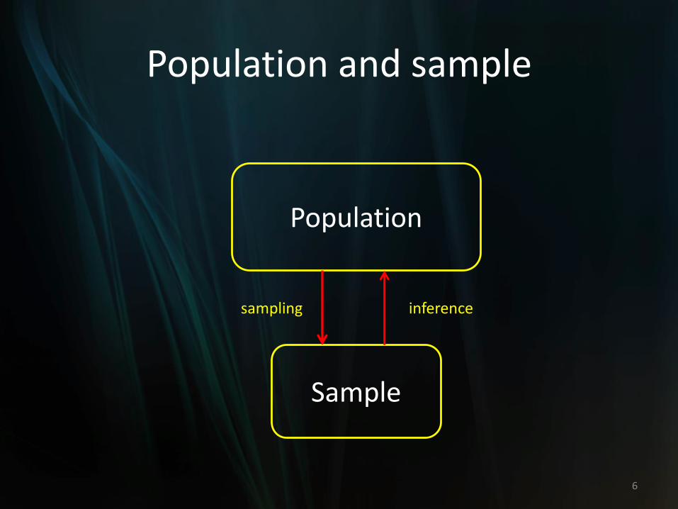
• We are much more interested in the population from which the sample was drawn.
– Example: 30 GPAs as a representative sample drawn from the population of GPAs of the freshmen currently in attendance at a certain university or the population of freshmen attending colleges similar to a certain university.
5
Population and sample
6
Population
Sample
sampling inference
Types of measurement
• Discrete: Quantitative data are called discrete if the sample space contains a finite or countably infinite number of values.
–How many days did you smoke during the last 7 days
7
Types of measurement
• Continuous: Quantitative data are called continuous if the sample space contains an interval or continuous span of real numbers.
–Weight, height, temperature
–Height: 1.72 meters, 1.7233330 meters
8
Types of measurement
• Nominal
–Categorical variables. Numbers that are simply used as identifiers or names represent a nominal scale of measurement such as female vs. male.
9
Types of measurement
• Ordinal
–An ordinal scale of measurement represents an ordered series of relationships or rank order. Likert-type scales (such as "On a scale of 1 to 10, with one being no pain and ten being high pain, how much pain are you in today?") represent ordinal data.
10
Types of measurement
• Interval: A scale that represents quantity and has equal units but for which zero represents simply an additional point of measurement. – The Fahrenheit scale is a clear example of the
interval scale of measurement. Thus, 60 degree Fahrenheit or -10 degrees Fahrenheit represent interval data.
11
Types of measurement
• Ratio: The ratio scale of measurement is similar to the interval scale in that it also represents quantity and has equality of units. However, this scale also has an absolute zero (no numbers exist below zero). For example, height and weight.
12
Types of measurement
• Qualitative vs. Quantitative variables
–Qualitative variables: values are texts (e.g.,Female, male), we also call them string variables.
–Quantitative variables: are numeric variables.
Basic statistics
• Two types of statistics
–Descriptive statistics
–Inferential statistics
14
Basic statistics
• Descriptive statistics:
–“are procedures used to summarize, organize, and make sense of a set of scores or observations.”
15
Basic statistics
• Inferential statistics:
–“are procedures used that allow researchers to infer or generalize observations made with samples to the larger population from which they were selected.”
16
Descriptive statistics
• Use descriptive statistics to describe, summarize, and organize set of measurements.
• Use descriptive statistics to communicate with other researchers and the public.
• Descriptive statistics: Central tendency and Dispersion
17
Descriptive statistics
• Measures of Central tendency: we use statistical measures to locate a single score that is most representative of all scores in a distribution.
–Mean
–Median
–Mode
18
Descriptive statistic
• The notations used to represent population parameters and sample statistics are different.
–For example
•Population size : N
• Sample size : n
19
Descriptive statistics
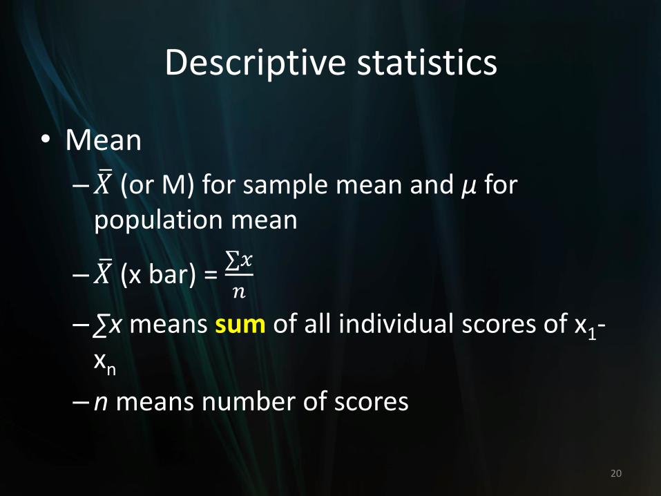
• Mean
– 𝑋 (or M) for sample mean and μ for population mean
– 𝑋 (x bar) = ∑𝑥
𝑛
–∑x means sum of all individual scores of x1-xn
–n means number of scores
20
Descriptive statistics
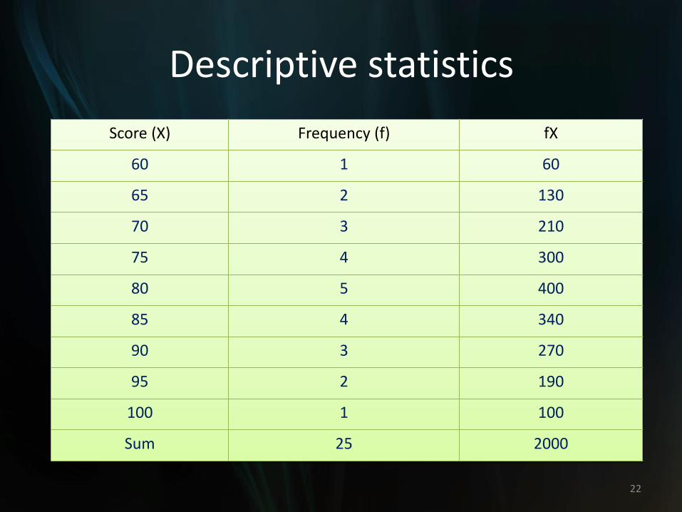
• Example 1: we want to know how 25 students performed in math tests.
• Data are in the next slide.
21
Descriptive statistics
22
Score (X) Frequency (f) fX
60 1 60
65 2 130
70 3 210
75 4 300
80 5 400
85 4 340
90 3 270
95 2 190
100 1 100
Sum 25 2000
Descriptive statistics
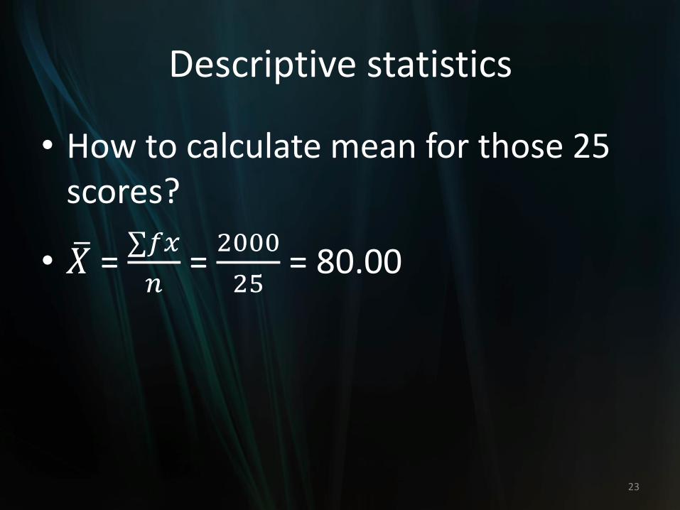
• How to calculate mean for those 25 scores?
• 𝑋 = ∑𝑓𝑥
𝑛= 2000
25= 80.00
23
Descriptive statistics
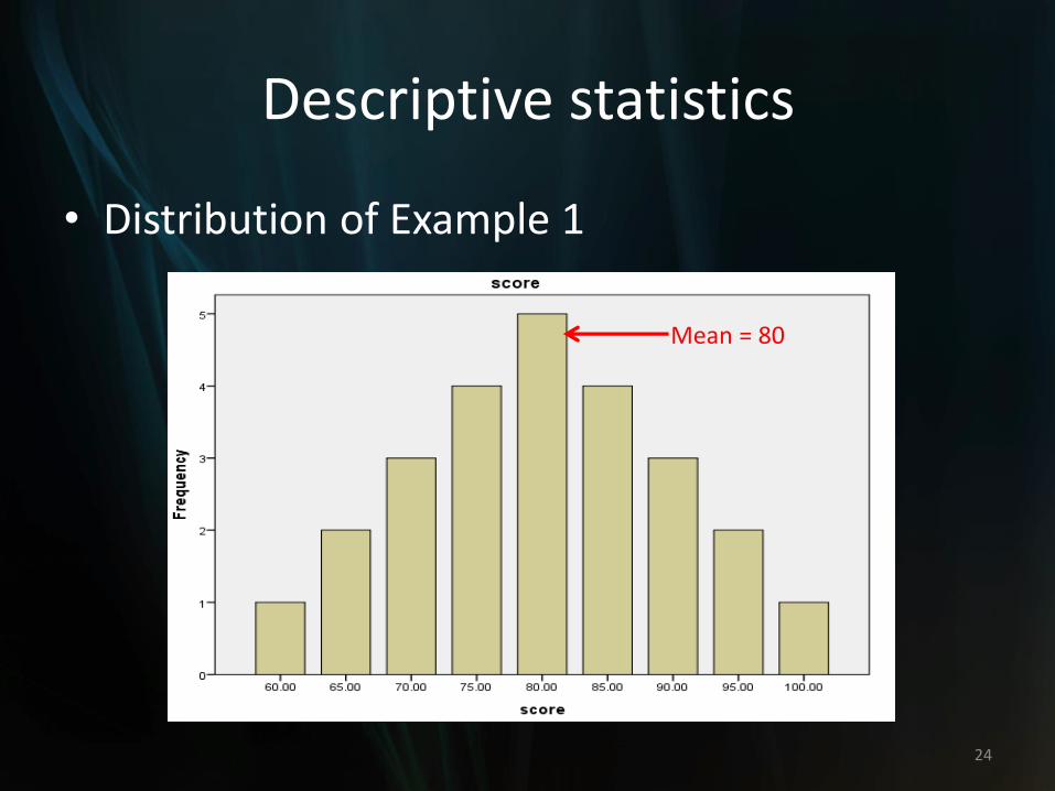
• Distribution of Example 1
24
Mean = 80
Descriptive statistics
• Median
–Data: 2, 3, 4, 5, 7, 10, 80. Mean of those scores is 15.86.
–80 is an outlier.
–Mean fails to reflect most of the data. We use median instead of mean to remove the influence of an outlier.
–Median is the middle value in a distribution of data listed in a numeric order.
25
Descriptive statistics
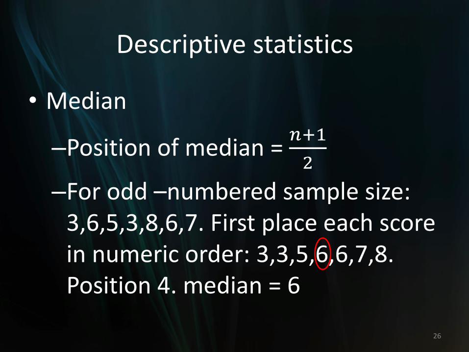
• Median
–Position of median = 𝑛+1
2
–For odd –numbered sample size: 3,6,5,3,8,6,7. First place each score in numeric order: 3,3,5,6,6,7,8. Position 4. median = 6
26
Descriptive statistics
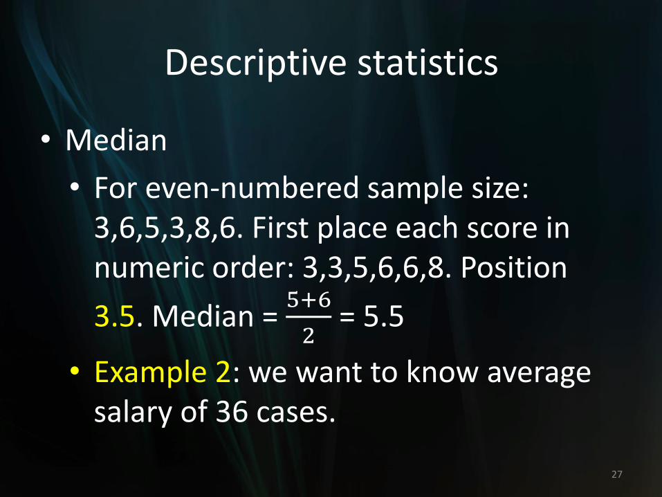
• Median
• For even-numbered sample size: 3,6,5,3,8,6. First place each score in numeric order: 3,3,5,6,6,8. Position
3.5. Median = 5+6
2= 5.5
• Example 2: we want to know average salary of 36 cases.
27
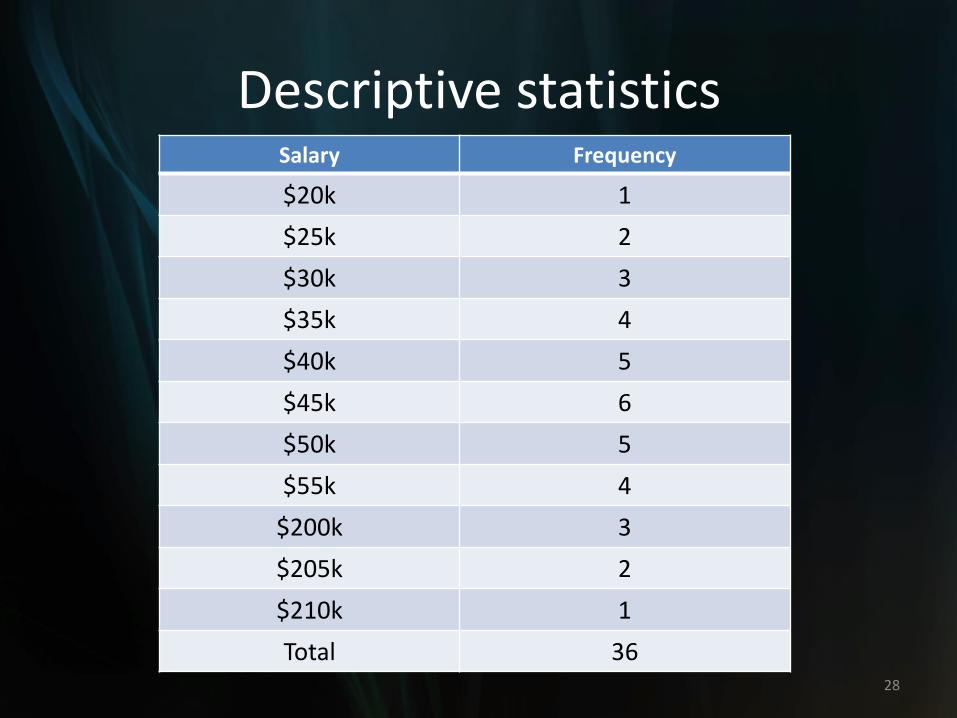
Descriptive statisticsSalary Frequency
$20k 1
$25k 2
$30k 3
$35k 4
$40k 5
$45k 6
$50k 5
$55k 4
$200k 3
$205k 2
$210k 1
Total 3628
Descriptive statistics
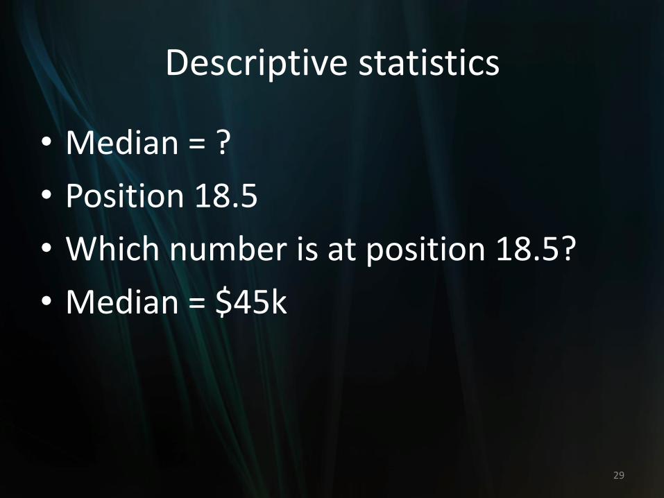
• Median = ?
• Position 18.5
• Which number is at position 18.5?
• Median = $45k
29
Descriptive statistics
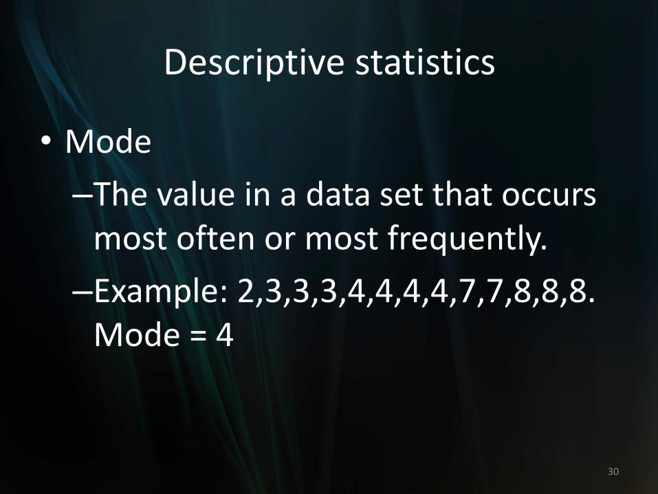
• Mode
–The value in a data set that occurs most often or most frequently.
–Example: 2,3,3,3,4,4,4,4,7,7,8,8,8. Mode = 4
30
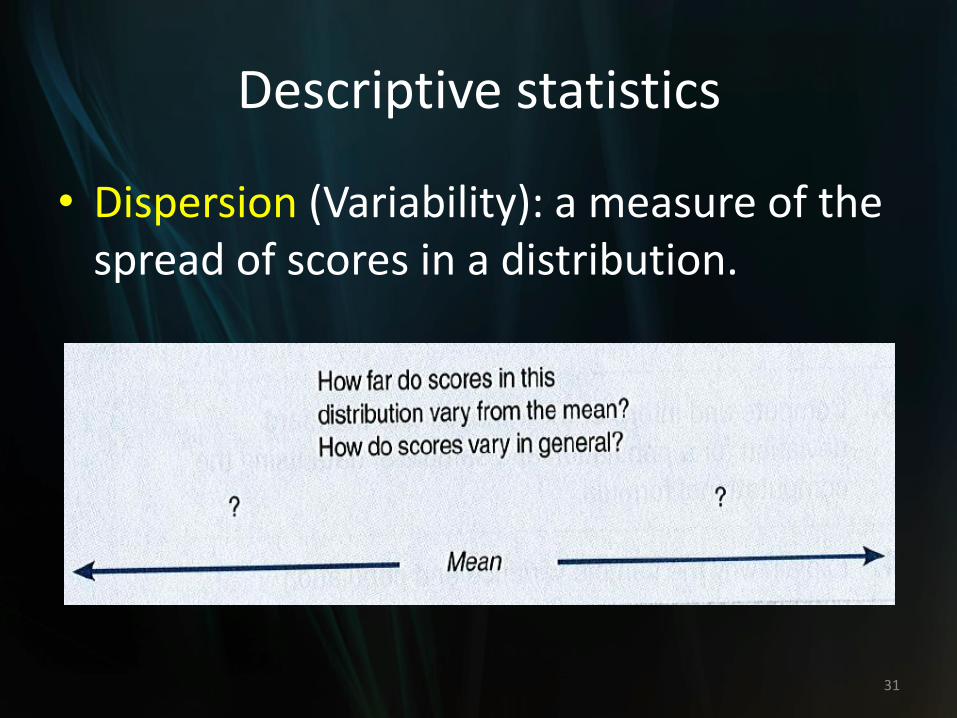
Descriptive statistics
• Dispersion (Variability): a measure of the spread of scores in a distribution.
31
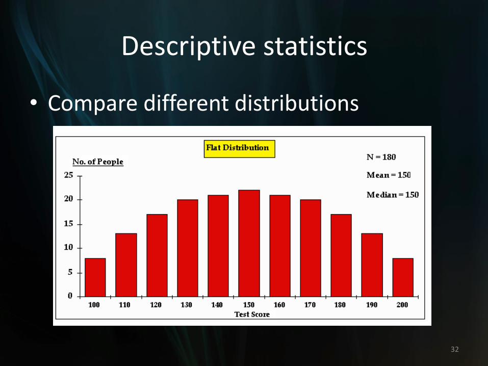
Descriptive statistics
• Compare different distributions
32
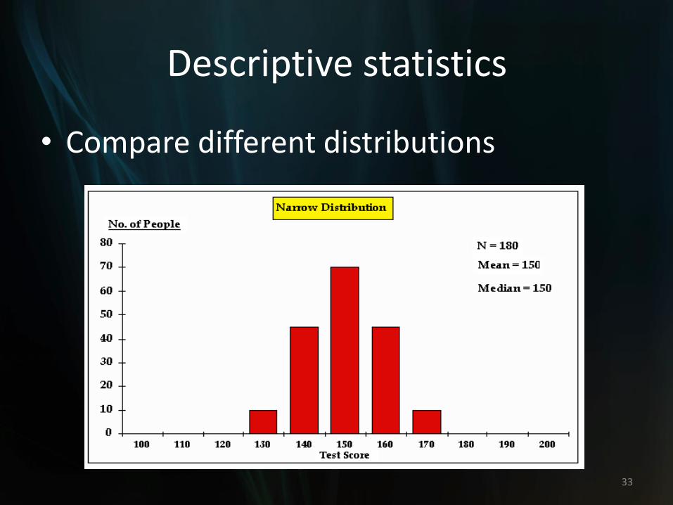
Descriptive statistics
• Compare different distributions
33
Descriptive statistics
• Two sets of data have the same sample size, mean, and median.
• But they are different in terms of variability.
34
Descriptive statistics
• Dispersion
–Range
–Variance
–Standard deviation
35
Descriptive statistics
• Range
–It is the difference between the largest value and smallest value.
–It is informative for data without outliers.
36
Descriptive statistics
• Variance
–It measures the average squareddistance that scores deviate from their mean.
–Sample variance: s2 (population variance σ2 sigma)
37
Descriptive statistics
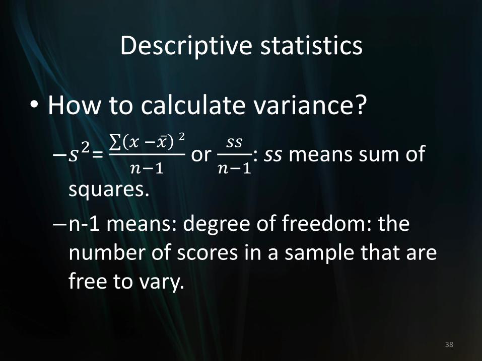
• How to calculate variance?
–𝑠2= ∑ 𝑥 − 𝑥 2
𝑛−1or
𝑠𝑠
𝑛−1: ss means sum of
squares.
–n-1 means: degree of freedom: the number of scores in a sample that are free to vary.
38
Descriptive statistics
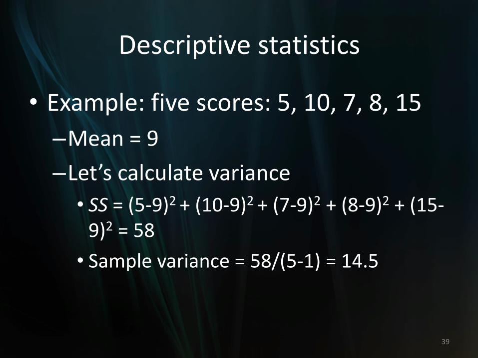
• Example: five scores: 5, 10, 7, 8, 15
–Mean = 9
–Let’s calculate variance
• SS = (5-9)2 + (10-9)2 + (7-9)2 + (8-9)2 + (15-9)2 = 58
• Sample variance = 58/(5-1) = 14.5
39
Descriptive statistics
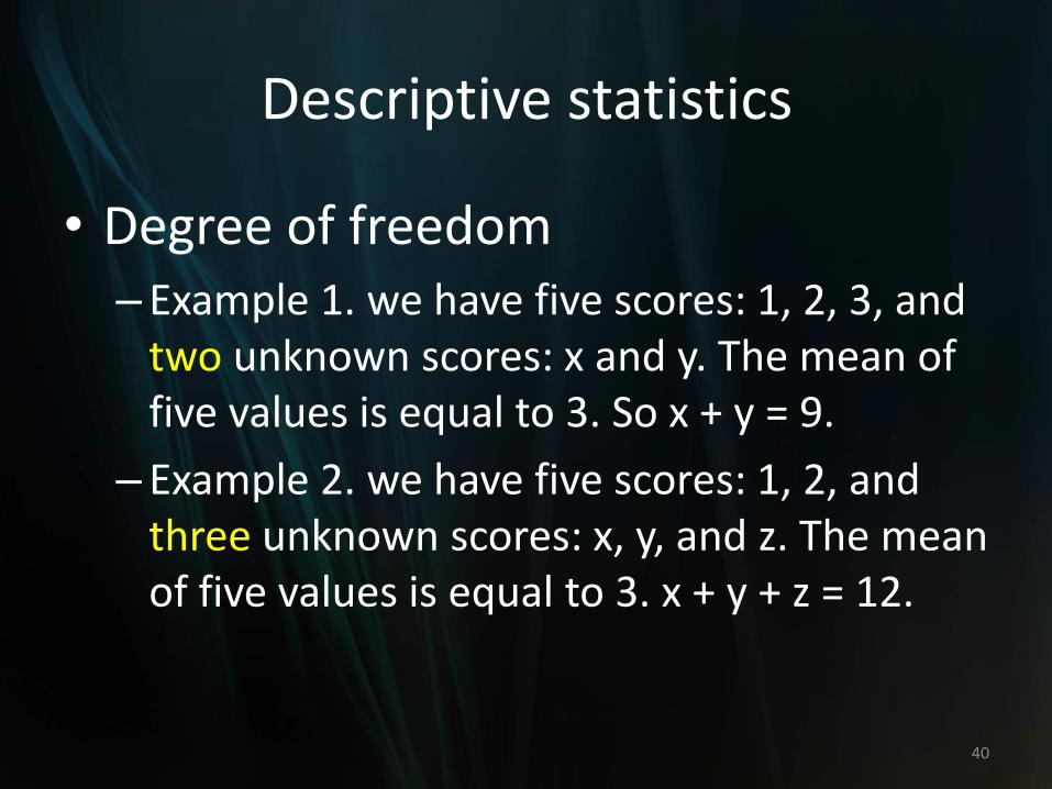
• Degree of freedom– Example 1. we have five scores: 1, 2, 3, and
two unknown scores: x and y. The mean of five values is equal to 3. So x + y = 9.
– Example 2. we have five scores: 1, 2, and three unknown scores: x, y, and z. The mean of five values is equal to 3. x + y + z = 12.
40
Descriptive statistics
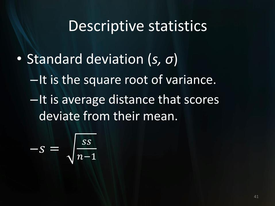
• Standard deviation (s, σ)
–It is the square root of variance.
–It is average distance that scores deviate from their mean.
–𝑠 =𝑠𝑠
𝑛−1
41
Descriptive statistics
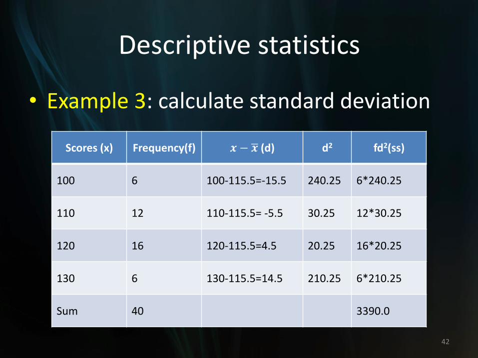
• Example 3: calculate standard deviation
42
Scores (x) Frequency(f) 𝒙 − 𝒙 (d) d2 fd2(ss)
100 6 100-115.5=-15.5 240.25 6*240.25
110 12 110-115.5= -5.5 30.25 12*30.25
120 16 120-115.5=4.5 20.25 16*20.25
130 6 130-115.5=14.5 210.25 6*210.25
Sum 40 3390.0
Descriptive statistics
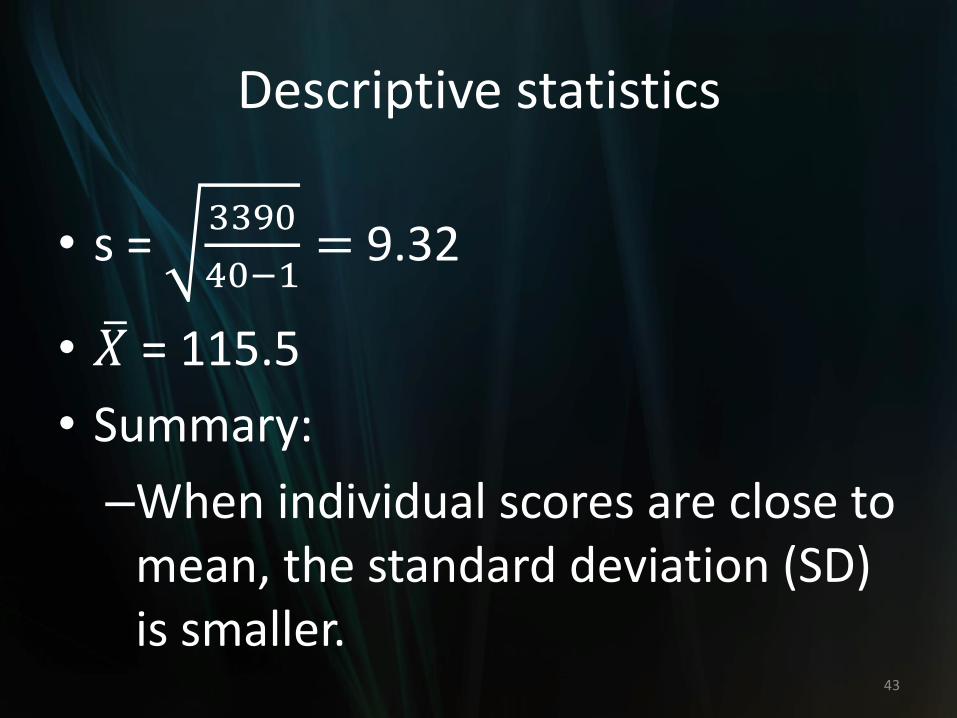
• s = 3390
40−1= 9.32
• 𝑋 = 115.5
• Summary:
–When individual scores are close to mean, the standard deviation (SD) is smaller.
43
Descriptive statistics
• Summary
–When individual scores are spread out far from the mean, the standard deviation is larger.
–SD is always positive
–It is typically reported with mean.
44
Descriptive statistics
• Choosing proper measure of central tendency depends on:
–the type of distribution
–the scale of measurement
45
Descriptive statistics
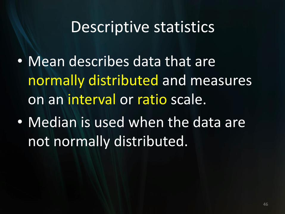
• Mean describes data that are normally distributed and measures on an interval or ratio scale.
• Median is used when the data are not normally distributed.
46
Descriptive statistics
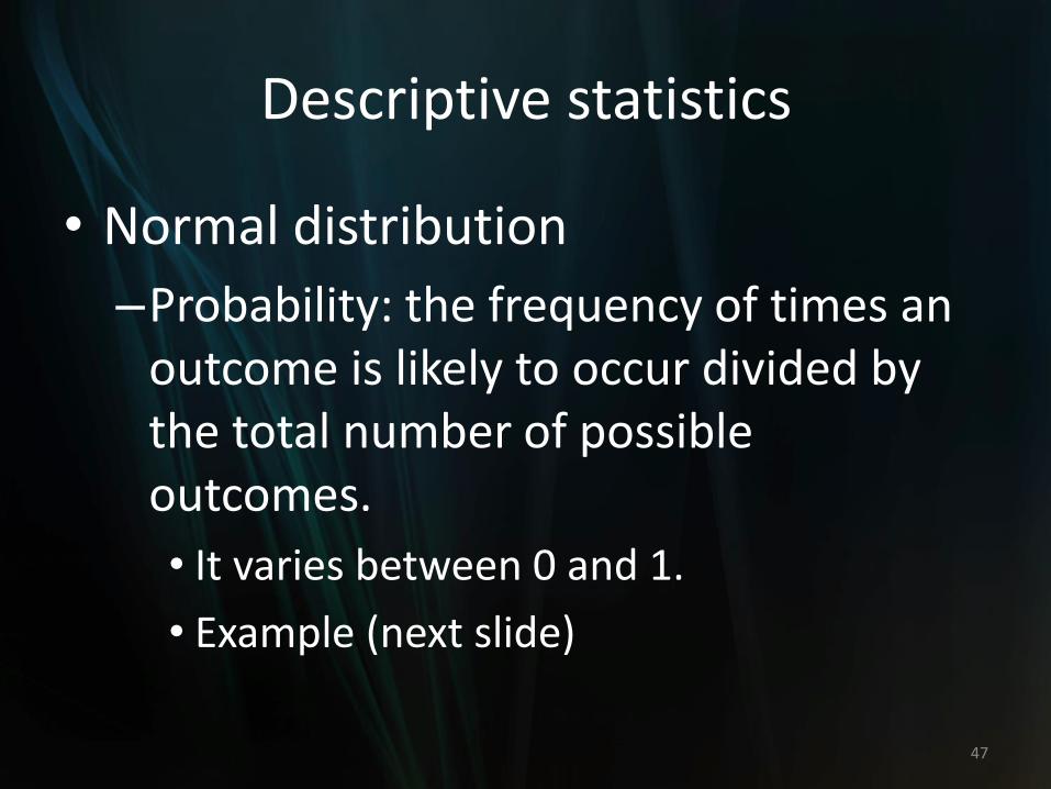
• Normal distribution
–Probability: the frequency of times an outcome is likely to occur divided by the total number of possible outcomes.
• It varies between 0 and 1.
• Example (next slide)
47
Descriptive statistics
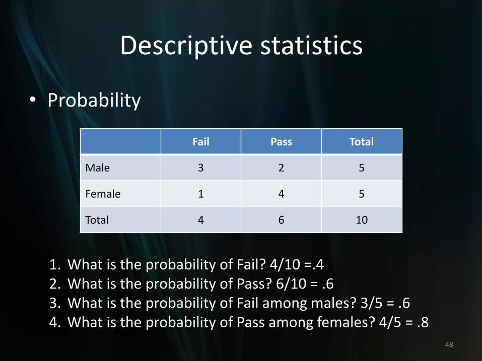
• Probability
48
Fail Pass Total
Male 3 2 5
Female 1 4 5
Total 4 6 10
1. What is the probability of Fail? 4/10 =.42. What is the probability of Pass? 6/10 = .63. What is the probability of Fail among males? 3/5 = .64. What is the probability of Pass among females? 4/5 = .8
Descriptive statistics
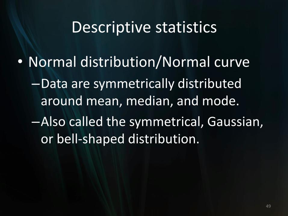
• Normal distribution/Normal curve
–Data are symmetrically distributed around mean, median, and mode.
–Also called the symmetrical, Gaussian, or bell-shaped distribution.
49
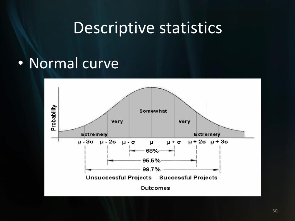
Descriptive statistics
• Normal curve
50
Descriptive statistics
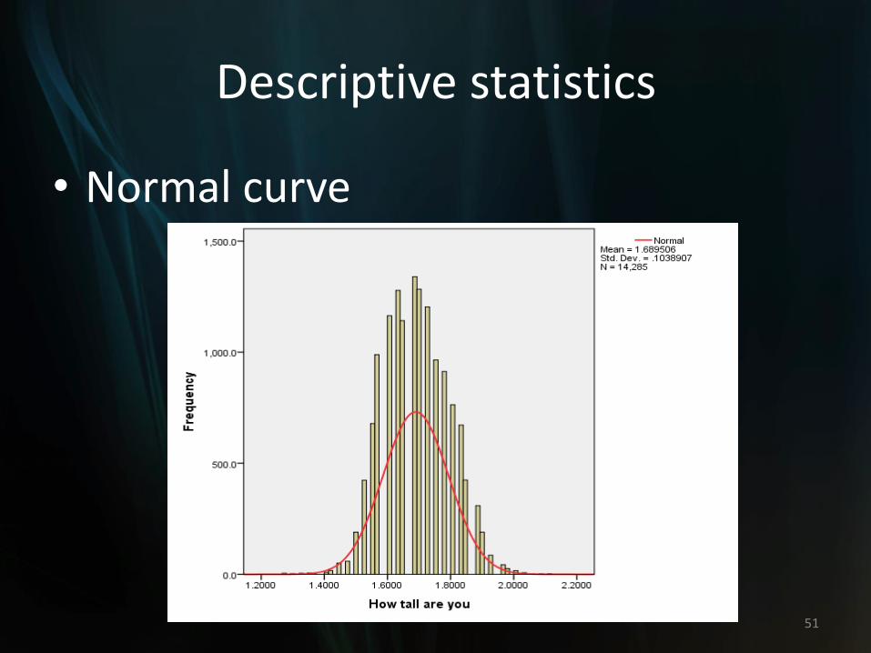
• Normal curve
51
Descriptive statistics
• Characteristics of normal distribution
–The normal distribution is mathematically defined.
–The normal distribution is theoretical.
–The mean, median, and mode are all the same value at the center of the distribution.
52
Descriptive statistics
• Characteristics of normal distribution
–The normal distribution is symmetrical.
–The form of a normal distribution is determined by its mean and standard deviation.
–Standard deviation can be any positive value.
53
Descriptive statistics
• Characteristics of normal distribution
–The total area under the curve is equal to 1.
–The tails of normal distribution are always approaching to x axis, but never touch it.
54
Descriptive statistics
• Normal distribution/Normal curve
–We use normal distribution to locate probabilities for scores.
–The area under the curve can be used to determine the probabilities at different points.
55
Descriptive statistics
56
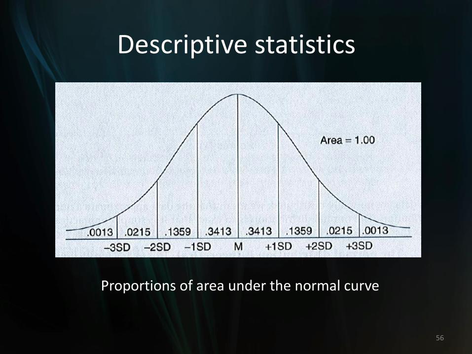
Proportions of area under the normal curve
Descriptive statistics
• Normal distribution: the standard deviation indicates precisely how the scores are distributed. Empirical rule:
–About 68% of all scores lie within onestandard deviation of the mean. In another word, roughly two thirds of the scores lie between one standard deviation on either side of the mean.
57
Descriptive statistics
• Normal distribution
–About 95% of all scores lie within twostandard deviation of the mean (Normal scores: close to the mean).
–About 99.7% of all scores lie within three standard deviation of the mean.
58
Descriptive statistics
• In another word, we have 95% chance of selecting a score that is within 2 standard deviation of mean.
• Less than 5% scores are far from the mean (NOT normal scores).
59

Descriptive statistics
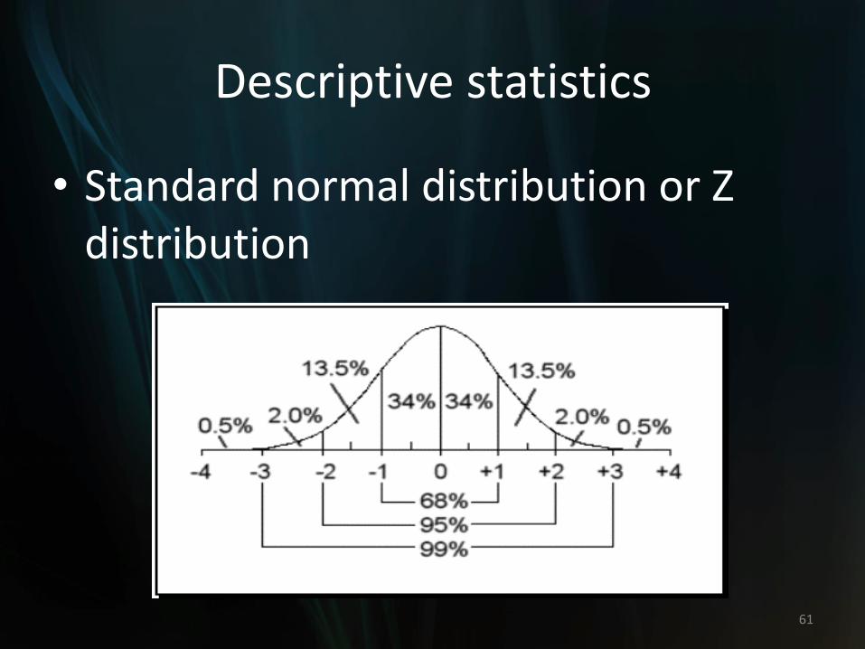
• Standard normal distribution or Z distribution
–A normal distribution with mean = 0, and standard deviation = 1.
–A Z score is a value on the x-axis of a standard normal distribution
60
Descriptive statistics
• Standard normal distribution or Z distribution
61
Descriptive statistics
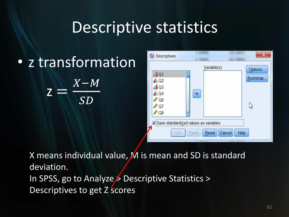
• z transformation
z =𝑋−𝑀
𝑆𝐷
62
X means individual value, M is mean and SD is standard deviation. In SPSS, go to Analyze > Descriptive Statistics > Descriptives to get Z scores
Descriptive statistics
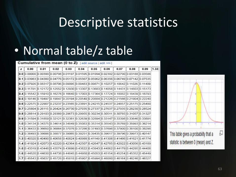
• Normal table/z table
63
Descriptive statistics
• How to use z table?
–Example: a sample of scores are approximately distributed normally with mean 8 and standard deviation 2. What is the probability of score lower than 6?
64
Descriptive statistics
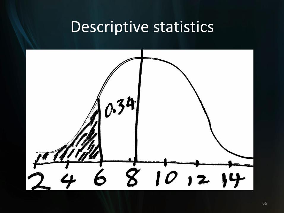
• How to use z table?
–Transform a raw score 6 into a z score
–z = (6-8)/2=-1
–Check the normal table p (probability) = 0.5-0.34=0.16
–The probability of obtaining score less than 6 is 16%
65
Descriptive statistics
66
Descriptive statistics
• Descriptive statistics in SPSS
–Frequencies
–Descriptives
–Explore
67
Descriptive statistics
• Exercise: use 2015 YRBSS data
–Use Explore function to get descriptive statistics for Q6 (height)
–Analyze > Descriptive Statistics > Explore
68
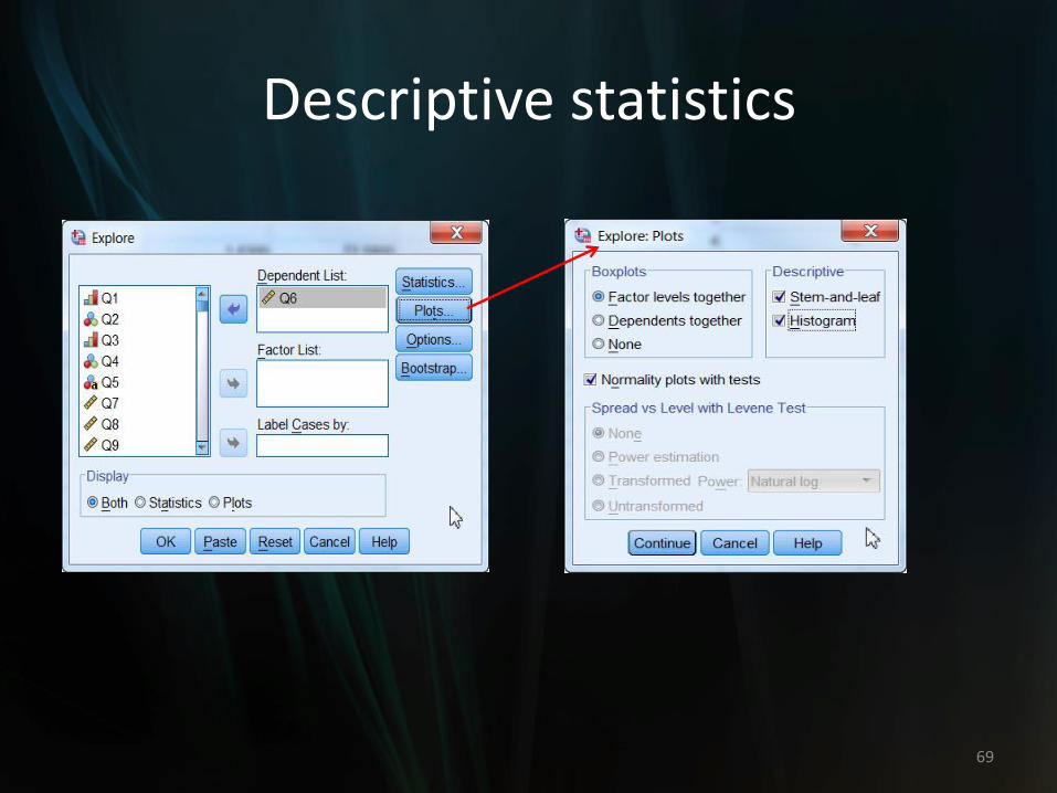
Descriptive statistics
69
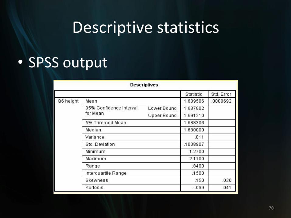
Descriptive statistics
• SPSS output
70
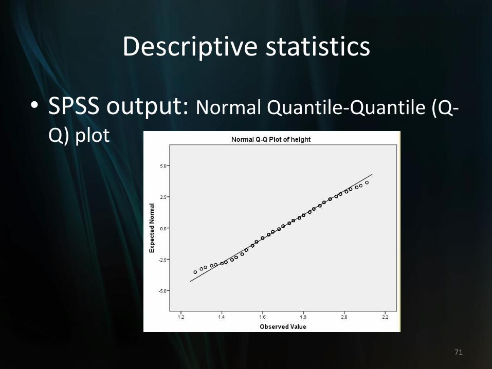
Descriptive statistics
• SPSS output: Normal Quantile-Quantile (Q-
Q) plot
71
Graphs
• Summarize quantitative data graphically
– It depends on the type of data
• Histogram: we use Histogram to summarize discrete data
72
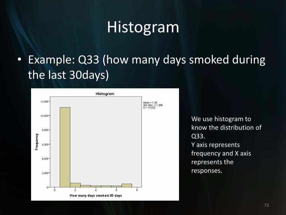
Histogram
• Example: Q33 (how many days smoked during the last 30days)
73
We use histogram to know the distribution of Q33. Y axis represents frequency and X axis represents the responses.
Scatter Plot
• We use scatter plot to check linear relationship between two scale variables
• Example: Q6 (height) and Q7 (weight) by Q2 (gender)
74
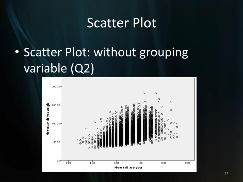
Scatter Plot
• Scatter Plot: without grouping variable (Q2)
75
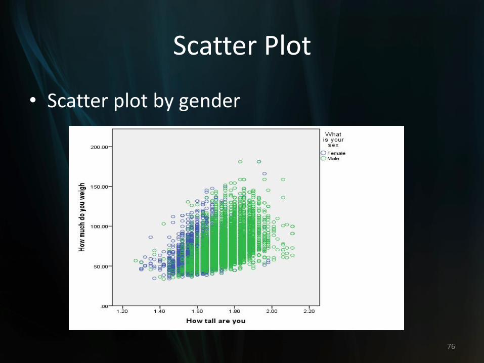
Scatter Plot
• Scatter plot by gender
76
Box Plot
• We can use either Explore function or Graphs to get box plot
• Example: box plot for Q6 (height) by Q2 (gender)
77

Box Plot
78
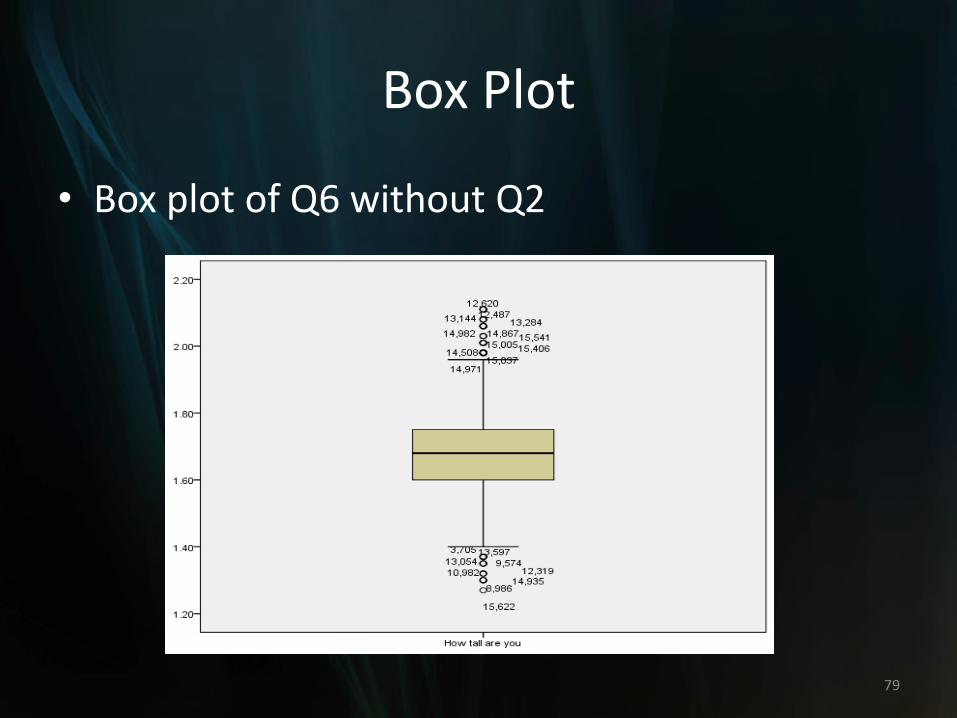
Box Plot
• Box plot of Q6 without Q2
79
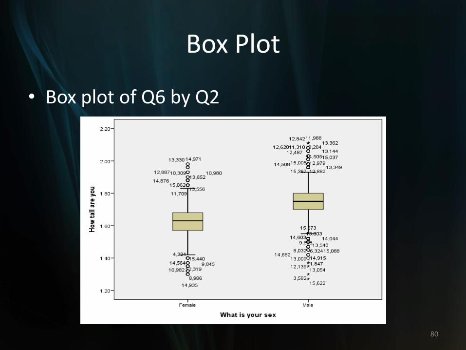
Box Plot
• Box plot of Q6 by Q2
80
Normal Q-Q plot
• Normal Q-Q plot or quantile-quantile plot
• We use Normal Q-Q plot to check normality assumption: we assume that Q6 is normally distributed.
• If the data indeed follow the normal distribution, then the points on the Q-Q plot will fall approximately on a straight line.
81
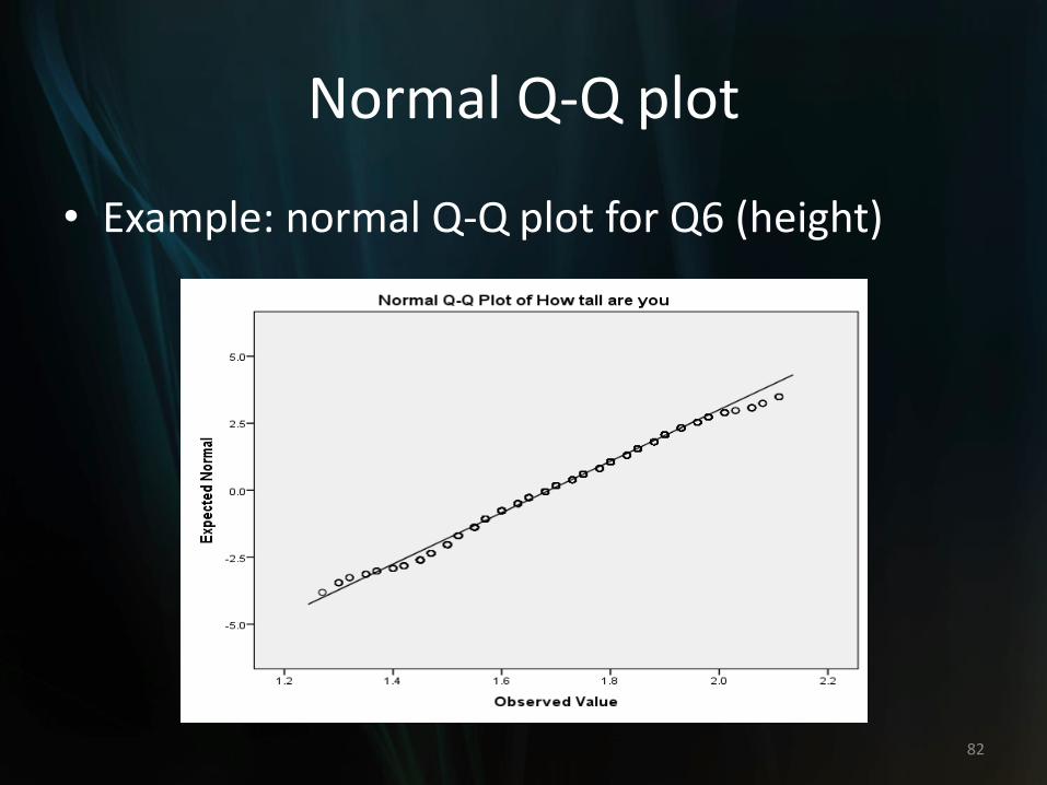
Normal Q-Q plot
• Example: normal Q-Q plot for Q6 (height)
82
Basic statistics
• References
–Agresti, A. & Finlay, B. (1997). Statistical methods for the social sciences. Upper Saddle River, NJ. Prentice Hall, Inc.
–Neutens, J. J., & Rubinson, L. (1997). Research techniques for the health sciences. Needham Heights, MA. Allyn & Bacon.
83
Basic statistics
• References
–Privitera, G. J. (2012). Statistics for the behavioral sciences. Thousand Oaks, CA. SAGE Publications, Inc.
84