Economic Theory and ForecastingOccasionally this Review publishes articles of a more technical nature.

These articles result from basic research efforts of staff economists.

It!0dUC1.jUii

I HE ECONOMIC FORECASTS for 1967 havebeen duly recorded and only await the passage oftime to see how accurate they were. This article doesnot attempt to add an additional forecast to those al-ready made. Rather, it specifies some of the commonunderlying assumptions or theories which majorgroups of forecasters accept and which they implicit-ly or explicitly take into account in constructing aforecast.

It is hoped that this review of forecasting as-sumptions will help clarify some of the differenceswhich separate those who forecast a substantial de-cline in the growth of gross national product (GNP)in 1967, with a resulting increase in unemployment,from those who project a high rate of growth in GNPand a continued tight labor market.

There is widespread interest in economic forecast-ing. It is of concern to the private citizen because ofthe information it may provide regarding his futureincome and employment. It is of interest to businessfirms which desire to plan their investment and pro-duction programs appropriately. It is of interest to theGovernment because its policy actions can affect thelevel of economic activity. Policymakers have someidea of a socially desirable level of economic activity.An accurate forecast tells what the actual level ofeconomic activity is most likely to be. ‘When actualand desired levels differ, appropriate application ofmonetary, fiscal, or other public policy may serve tomove the actual closer to the desired value.

Empirical Earccast.s

Methods of economic forecasting may be divided in-to two major classes. One class uses primarily an em-pirical approach, while the other class combineseconomic theory with empirical evidence. The best-known empirical approach to forecasting is the lead-ing indicators” technique. This was originally devel-oped by the National Bureau of Economic Research(NBER) during the 1920’s, and since 1961 data forapplying this technique have been published monthly

by the Department of Commerce in Business CycleDevelopments. This technique consists of examininga wide range of economic data from previous businesscycles to discover those time series which typicallyshow peaks and troughs before peaks and troughsare observed in general business conditions.

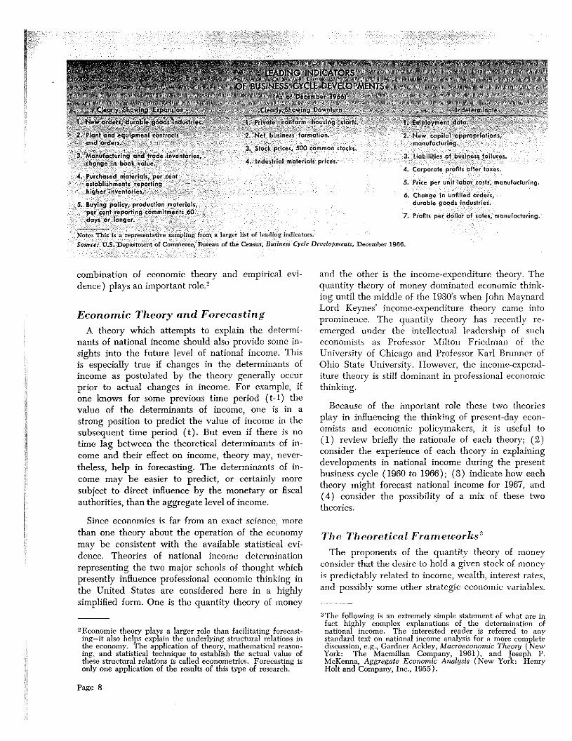
The leading indicators approach is widely reportedand discussed in the financial press. In the December1966 issue of Business Cycle Developments (which pre-sented the best information then available, when mostforecasts of 1967 were being completed), the leadingindicators were giving conflicting evidence about thefuture. A sampling of leading indicators published inthe December issue is presented in the accompanyingtable. Some indicators showed continued expansion,others had turned down, and many were indeter-minate. For example, in the last half of 1966 neworders received by durable goods industries andplant and equipment contracts and orders tended toincrease at about the same rate as during the wholeof the 1961-66 expansion period. By comparison, pri-vate nonfarm housing starts and stock market prices,two other leading indicators, showed well-publicizeddecreases. (Since December the stock market hasshown renewed strength.) Also, many of the “coin-cident indicators,” those which generally move simul-taneously with peaks and troughs in business cycles,registered advances. Given this conflicting evidenceplus uncertainties regarding Government spendingfor Vietnam, it is not surprising that there was a con-siderable degree of uncertainty in the projections ofmany forecasters.’

To evaluate the mass of largely conflicting evidenceavailable to forecasters, some judgment about whatare important and what are secondary causes ofchanges in the economy are needed. It is in thiscontext that the second class of forecasting tools (the

Some attempts have been made to apply an objective statis-tical test to see if a mixture of leading and coincident indica-tors point to continued expansion or contraction. For example,see Leonall C. Andersen, “A Method of Using DiffusionIndexes to Indicate the Direction of National EconomicActivity,” 1966 Proceedings of the Business and EconomicStatistics Section, American Statistical Association (Washington,D.C.), pp. 424-434.

Page 7

,rm

..J eç.~ipr..entcontra~.. 2. Net business formation. 2. New copilot appropriations,t den. . manufacturing.

3. Slack prices, 500 commor. slacks.3. Manufacturing and trade inventories, . . . 3. Liabilities of business faiurcs.

change in book value. 4. Industrial materials prices.4. corporate profits after taxes.

4. Purchased materials, per centestablishments reporting 5. Price per unit labar costs, manufcicturirsg.higher inventories.

6. Change in unfilled orders,5. Buying policy, production materials, du’ob’e goods industrias.

per cent reporting commitments 60days or longer. 7. Prafits per dal,ar of sales, manufacturing

Note: ‘rbis isursprtsesst.ttnt’ ,.ssr.pling from a l.irg.’r hI r,f Ii’ sih, ‘r sss(.r..caurre: tl.S. Dcii irtnstsit of Cs’mrn, tee. Btsrc’sss tsf tist’ C vncss’• Busi,,en Cd. D, , aof.mcni 5, I ). c,’ss’.l ii’ 199fi.

combination of economic theory and empirical evi-dence) plays an important role.2

Economic Theory and Forecasting

A theory which attempts to explain the determi-nants of national income should also provide some in-sights into the future level of national income. Thisis especially true if changes in the determinants ofincome as postulated by the theory generally occurprior to actual changes in income. For example, ifone knows for some previous time period (t-1) thevalue of the determinants of income, one is in astrong position to predict the value of income in thesubsequent time period (t). But even if there is notime lag between the theoretical determinants of in-come and their effect on income, theory may, never-theless, help in forecasting. The determinants of in-come may be easier to predict, or certainly moresubject to direct influence by the monetary or fiscalauthorities, than the aggregate level of income.

Since economics is far from an exact science, morethan one theory about the operation of the economymay be consistent with the available statistical evi-dence. Theories of national income determinationrepresenting the two major schools of thought whichpresently influence professional economic thinking inthe United States are considered here in a highlysimplified form. One is the quantity theory of money

2 theory plays a larger role than facilitating forecast-ing—it also helps explain the underlying structural relations inthe economy. The application of theory, mathematical reason-ing, and statistical technique to establish the actual value ofthese structural relations is called econometrics. Forecasting isonly one application of the results of this type of research.

and the other is the income-expenditure theory. Thequantity theory of money dominated economic think-ing until the middle of the 1930’s when John MaynardLord Keynes’ income-expenditure theory came intoprominence. The quantity theory has recently re-emerged under the intellectual leadership of sucheconomists as Professor Milton Friedman of theUniversity of Chicago and Professor Karl Brunner ofOhio State University. However, the income-expend-iture theory is still dominant in professional economicthinking.

Because of the important role these two theoriesplay in influencing the thinking of present-day econ-omists and economic policymakers, it is useful to(1) review briefly the rationale of each theory; (2)consider the experience of each theory in explainingdevelopments in national income during the presentbusiness cycle (1960 to 1966); (3) indicate how eachtheory might forecast national income for 1967, and(4) consider the possibility of a mix of these twotheories.

The Theoretical Frameworks3

The proponents of the quantity theory of moneyconsider that the desire to hold a given stock of moneyis predictably related to income, wealth, interest rates,and possibly some other strategic economic variables.

3The following is an extremely simple statement of what are infact highly complex explanations of the determination ofnational income, The interested reader is referred to anystandard text on national income analysis for a more completediscussion, e.g., Gardner Aekley, Macroeconomic Theory (NewYork: The Macmillan Company, 1961), and Joseph P.Mc}Cenna, Aggregate Economic Analysis (New York: HenryHolt and Company, Inc., 1955).

I - Page8 -- -- -

4

Based on the value of these variables, all spending cause of changes in income. This is not only becauseunits are considered to desire a certain amount of

money to hold. This theory also postulates that dis-cretionary actions by the Federal Reserve can alterthe actual stock of money relative to the desiredstock, thereby setting into action a course of eventswhich leads to a change in income and interest rates.When the actual stock of money differs from the

desired stock, a response is induced on the part ofthe public to re-establish the desired relation. Thisattempt to shift between money and other financialassets or commodities affects interest rates and ag-gregate demand and through these the level of prices

and real output.

The income-expenditure theory divides expendituresinto two groups—those which are induced or aredependent on current income and those which areautonomous or are independent of current income.Most consumption spending is considered to dependupon income and is therefore the major induced ex-penditure. Autonomous expenditures (as defined inthis article) are investments of business firms, govern-

ment expenditures, the net export surplus, and someminor items.4 Although autonomous spending is inde-

pendent of current income, it is, of course, dependenton something. Government spending depends upon thepolicy decisions of the President, Congress, and theiradvisers; business investment depends upon suchfactors as expectations of future sales, changes intechnology, and interest rates; exports depend uponincome and prices in the rest of the world and the

exchange rate. By definition, the sum of induced andautonomous expenditures is equal to the total value ofall goods and services produced in the economy, i.e.,GNP. Thus, autonomous spending is one componentof CNP, but the level of GNP does not directly deter-mine the amount of autonomous spending.

The proponents of the income-expenditure theorypostulate that consumption expenditures are very

closely tied to the level of income and thus cannotgenerally act as a substantial initial cause of short-term changes in income.5 Consequently, changes inautonomous expenditures are considered the major

~There is considerable controversy among economists aboutwhich components of income are induced and which areautonomous. See Appendix, page 14, for some discussion ofthis and other issues.

5The income-expenditure theory considers certain exceptions in

Qthe dependence of consumption on income. (1) A sharchange in the public’s expectations about future prices or avai -

ability, such as took place in the early months of the KoreanWar, can temporarily increase the consumption-income relation

autonomous spending is a component of income, butalso (and more importantly) because autonomousspending actually induces changes in consumption.The Government, through its control of expenditures,affects the level of autonomous spending, thereby in-fluencing consumption and GNP.

The formal structure of each theoretical model ispresented in the following highly simplified equations:

Quantity Theory of Money

1. ~Y, n_—c + v (AM)tn

Income-Expenditure Theory

2. i~Y~= a + b (~A)tn

Money°Autonomous spendingtime unit which is one-quarter of a yeardifferent possible time lags between(M) and (Y) and between (A)and (Y)

~=. change between quarters

The symbols, c, v, a, b, represent specific statistical-ly determined values relating (M) to (Y) and (A)to (Y). The quantity theory of money (equation 1)says that short-term movements in GNP (a Y) arclargely determined by changes in the stock of money

aM). The income-expenditure theory (equation 2)says that changes in autonomous spending (~A) de-termine short-term movements in CNP (AY).7

(Continued from col. 1)

because of scare buying. (2) There may be a change in tastesof the public or temporary saturation of the market whichcould decrease consumption of some product although incomeis unchanged. The first factor has been sufficiently unpredict-able that it would be unprofitable to incorporate it into ageneral theory explaining consumption. The second factormay be of major importance in analyzing a particular com-modity market (like autos), but it has not been a major factorin causing changes in overall consumption.

°Several definitions of money are used in economic literature.The standard definition of money, which is used here, is cur-rency held outside of commercial banks plus demand depositsadjusted (referred to as Ml). Some economists consider thisdefinition too narrow because it excludes other impurtantsources of household and business liquidity. A broader defi-nition which is sometimes used is Ml plus time deposits incommercial banks (referred to as M2).

tThose economists who consider that both theories jointly ex-plain how GNP is determined might say that monetary vari-ables (through the interest rate) will affect autonomousspending, while autonomous variables (through demand forbank credit, etc.) will affect the money supply. According tothis view, independent changes in either money or autonomousvariables, or both, determine the level of GNP.

Page 9

Y= GNP

t=-:

t-n, t-m=

The obvious policy difference between the twotheories is that the first emphasizes the role of moneyand central bank monetary policy in determiningGNP, while the second emphasizes the role of auton-omous expenditures and Government fiscal policy indetermining GNP. In the event that movements inmoney and autonomous expenditures are in differentdirections, very different conclusions as to the futurecourse of GNP would be forecast by proponents ofeach of the theories.

A case in point is the recent economic experience inthis country. From the second to the fourth quarterof 1966 the economy experienced a period of tightmoney but a continuing stimulative fiscal policy. Theproponents of the quantity theory might reasonablyforecast for 1967 a marked decline in the growth ofGNP and real output. On the other hand, proponentsof the income-expenditure theory would most likelyexpect continued growth in GNP at a relatively rapidrate.

~ •.. & &....

One way to examine these theories is to comparemovements in GNP with each of the theoreticallypostulated determinants of GNP, i.e., money andautonomous spending, to see how closely each hasmoved with GNP. Because there are strong upwardtrends in money, GNP, consumption, and autono-mous spending, turning points in the data may noteasily be observed. To remove mostof the trend and therefore to con- Changescentrate on the cyclical elements in Billions of Dollars

income, its components, and money, 20

quarterly changes in each series areused.8 15

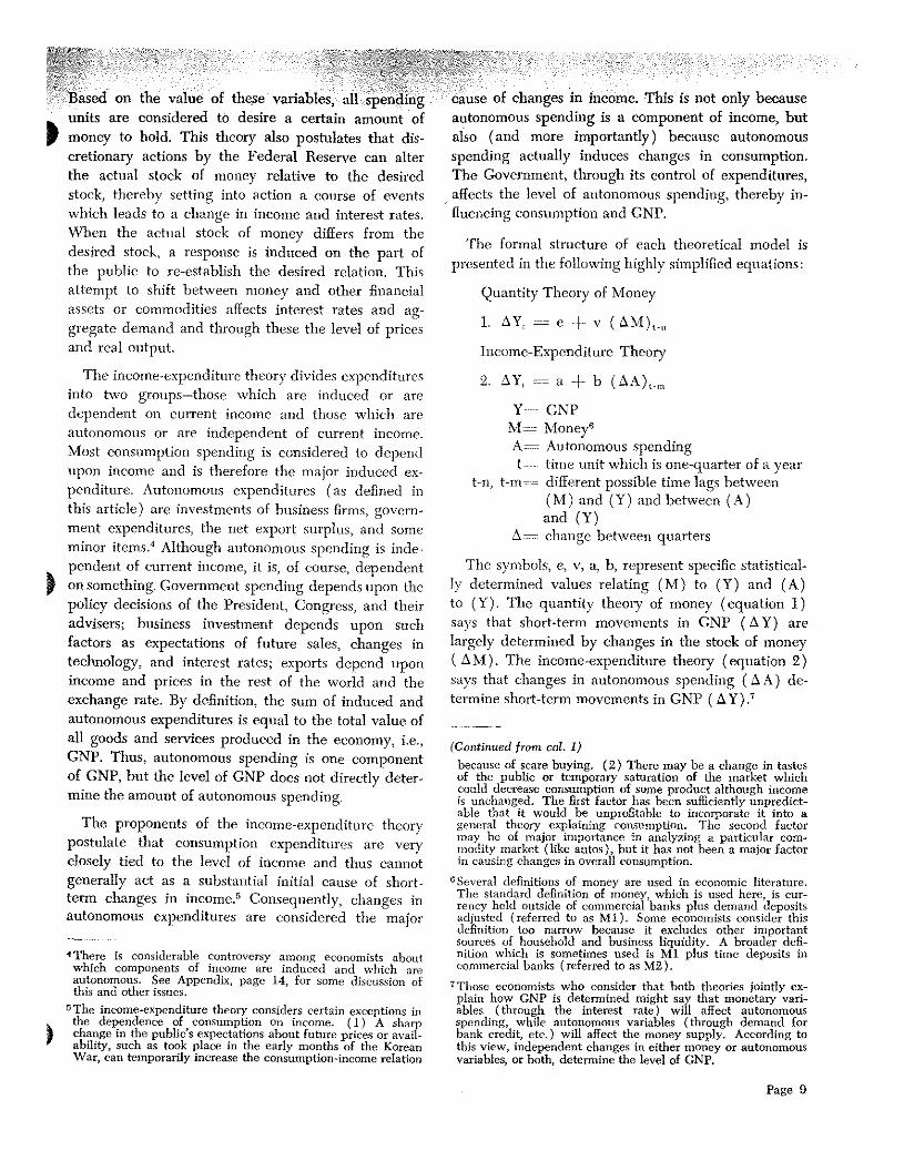
In Chart 1 quarterly changes inmoney and GNP are plotted from1958 (4th quarter) to 1966 (4thquarter). In Chart 2 quarterlychanges in autonomous spending

8The generally accepted convention incomputing changes for any time period(t) is to consider the difference between(t-1) and (t). However, there is nonecessary reason for this. The change at(t) could also be measured as the differ-ence between (t) and (t+1). The valueof the change at (t) used here is theaverage of these two measures of change.The practical advantage of this approachis that it reduces macli of the randonjstatistical “noise” (movement) which re-sults from the use of first differences com-putations.

Page 10

10

5

0

-5

10

U.

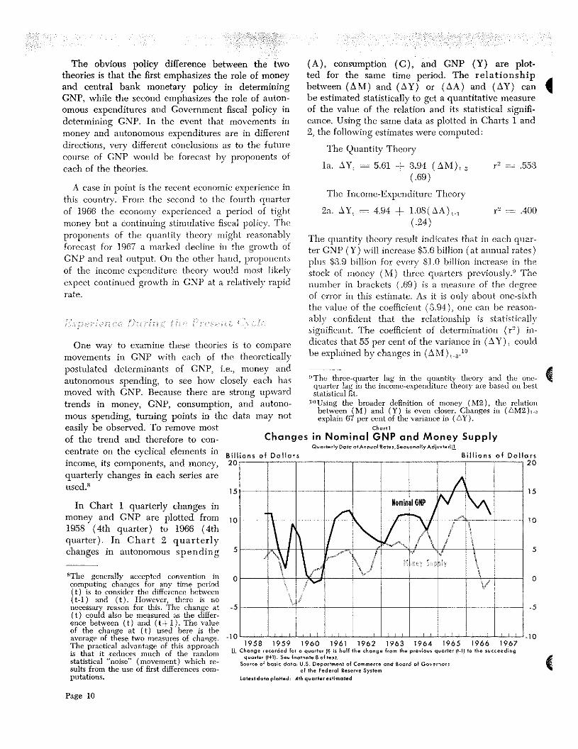
(A), consumption (C), and GNP (Y) are plot-ted for the same time period. The relationshipbetween (SM) and (~Y) or (AA) and (~Y) canbe estimated statistically to get a quantitative measureof the value of the relation and its statistical signifi-cance. Using the same data as plotted in Charts 1 and2, the following estimates were computed:

The Quantity Theory

la. ~ = 5.61 H- 3.94 (aM)1., r2 nr .553(.69)

The Income-Expenditure Theory

2a. aY~ 4.94 + 1.08(aA)1.1 r2 :.n .400(.24)

The quantity theory result indicates that in each quar-ter GNP (Y) will increase $5.6 billion (at annual rates)plus $3.9 billion for every $1.0 billion increase in thestock of money (M) three quarters previously.0 Thenumber in brackets (.69) is a measure of the degreeof error in this estimate, As it is only about one-sixththe value of the coefficient (3.94), one can be reason-ably confident that the relationship is statisticallysignificant. The coefficient of determination (r2) in-dicates that 55 per cent of the variance in (~Y) couldhe explained by changes in (AM)~.3.1°

0The three-quarter lag in the quantity theory and the one-quamter lag in the income-expenditure theory are based on beststatistical fit.

30Using the broader definition of money (M2), the relationbetween (M) and (Y) is even closer. Changes in (AMa),.,explain 67 per cent of the variance in (AY).

Chart 1

in Nominal GNP and Money SupplyQuarterly Data otAnnual Rates,SeasanalfyAdiu,tedij.

Billions of Doll o rs20

0

01958 1959 1960 1961 1962 1963 1964 1965 1966 1967

Change recorded for a quorter ftf is t,otl the change from the previous quarter It-f) to thesucc eedingquarter ft+lf. See toot,ore Sot text.

Source of basic doto: u.s. Deportment of Commerce and Board of Governorsol the Federal Reserve System

l.otestdota planed: 4th quarterestimated

Chort2

Changes in GNP, Consumption, and Autonomous SpendingQuortertyDoto otAenuolkates.SeanonolfyAdiusfedU.

Billions of Dollors GKP (Y) 2 Bflhions of Dollars20 20

15

10

5

0

-5

.1 ..l___i__J___.&

Aulonomous Spending(Al

to1958 1959 1960 1961 1962 1963 1964 1965

U. Chong erecor ded for a quarter if) is halt the change from the previous quarterquarter fit). See tootnote 8 of text

L~Y&&C+ASource of basic data: 3,5. Deportment of Commercetalentdata plooed: 4th quarterestim oted

fl The income-expenditure theory result indicates thatin each quarter GNP increases $4.9 billion plus $1.1

billion for every $1.0 billion increase in autonomousspending (A) in the previous quarter. This co-efficient is also statistically significant and 40 per centof the change in (~Y), can be explained by changesin (AA)~1.

In Charts 1 and 2 turning points can be observedin each series.1’ In Chart 1 the upper turning points, inthe money time series generally occur in the samequarter as the upper turning points in the incomeseries. On the other hand, the lower turning points inmoney lead the lower turning points in income bytwo to three quarters. One possible implication ofthis is that GNP responds promptly to a decline in amonetary variable but responds sluggishly to an in-crease. Even quite small movements in GNP appear tobe associated with small movements in money. Themoderate deceleration in money in the middle of1962 is related to the moderate deceleration in GNP inlate 1962 and early 1963. On the other hand, larger

“The turning points or peaks and troughs in the first differenceseries are not the same as business cycle turning points asdetermined by the National Bureau r,f Economic Research.NBER business cycle turning points are determined from a

O number of factors, hut they are influenced heavily by thelevel of income. One would expect the NBER turning pointsto occur after turning points described here because a decel-eration in income generally occurs before a decline in income.

I I

I I I

movements in GNP are associatedwith large movements in money.For example, the sharp decelerationin money in late 1959 and early1960 compared with a sharp de-celeration in GNP in mid- and late1960.

Changes in autonomous expen-ditures (A) are related to changesin CNP (Y) and consumption (C)

15 in Chart 2.” In this case there is

10 also a similarity between the move-ments in the time series, \vith (A)

~ slightly leading (C). The major de-0 ccleration in autonomous spending~ from the second quarter of 1960 to

15 the fourth quarter of 1960 com-_____ pares \vith the deceleration in con-10 sumption spending from the third

5 quarter of 1960 to the first quarter

o of 1961. The acceleration in auton-_____ _____ omous spending beginning in the1966 1967 first quarter of 1961 compares withthe succeeding the acceleration in consumption and

GNP from the second quarter of1961. Complementary movements

between these two series are observed for other timeperiods. There is, however, one case where a decelera-tion in autonomous spending (from the third quarterof 1962 to the first quarter of 1963) was not associatedwith any significant deceleration in the growth ofconsumption spending.

I ~&fl&6\P Forecasts

To forecast national income for 1967 on the basisof the two theoretical frameworks requires a projec-tion of the course of money and autonomous spend-ing during 1967. The best statistical fit observed be-tween money and GNP over the last eight years waswith changes in money three quarters before thechanges in GNP. Thus, on the basis of currently avail-able information the quantity theory would indicatethat, given the decline in the stock of money throughthe fourth quarter of 1966, it is highly probable therewill he a substantial slowdown in the growth of GNPat least until the third quarter of 1967. Given the stock

“We cannot compare statistically the relationship betweenautonomous spending (A) and CNP (Y) in the same timeperiod because (A) is a component of (Y). Variations inautonomous spending would lead to variations in income notbecause of the causal link postulated in the theory butbecause of a statistical artifact. To avoid this problem, (A)can either be related to the other component of incomewhich, in this case, is consumption spending (C), or (A)can be related to (Y) with a time lag. The second possibil-ity is considered here and the first is considered in theAppendix.

Page 11

15

10

5

0

-5

15

10

5

0

.5

15

10

5

0

.5

Given the way in which the quantity theory hasbeen stated here, there is no way of knowing how theincrease in GNP in 1967 will be distributed betweenprice increases and real increases. However, thereseems to be wide agreement that even svith a declinein the growth of GNP the inflationary momentumdeveloped in 1966 will carry over into 1967 in theform of cost-push, with average prices increasingabout 2.5 per cent. The growth in real output consist-ent with this calculation would be between 1.0 and1.5 per cent from the fourth quarter of 1966 to thefourth quarter of 1967, down substantially from the4.1 per cent growth for the same period in 1966. Thisforecast of 1967 growth in real GNP is below thegrowth in capacity, which is generally estimated atabout 4 per cent. This implies some increase in un-employment in 1967. Milton Friedman, a major ex-ponent of the quantity theory approach, has predicted(Newsweek, October 17, 1966 and January 9, 1967)that the U.S. economy would suffer a recession in 1967on the basis of the decline in the money supply in thelast half of 1966.

Forecasting 1967 GNP on the basis of the income-expenditure theory requires a projection of autono-mous spending through most of 1967. This is becausethe best statistical relation between changes in auton-omous spending (iSA) and GNP (~Y) is with a one-quarter time lag. To predict the course of GNP during1967 with only a one-quarter forecasting horizonrequires estimates of (~A)through the third quarterof 1967. Autonomous spending consists mainly ofbusiness investment and Government spending. Thisis why many forecasters emphasize the need to esti-mate these variables before any projection of GNP canbe attempted. If these estimates are unreliable, the

Page 12

According to the Department of Commerce-SECSurvey of Business Intentions released in December1966, investment in 1967 will be 7 per cent above the1966 level. The increase from the fourth quarter of1966 to the fourth quarter of 1967 will be smaller(perhaps a 4 per cent increase). On the other hand,Government spending, especially because of the Viet-nam War, is estimated in the budget to be about 13per cent or $16 billion higher in the fourth quarter of1967 than in the fourth quarter of 1966. The exportsurplus should also be larger. On the assumption ofno significant increase in tax rates,~the sum of allof this autonomous spending should grow at a healthy,though somewhat reduced, rate in 1967 as com-pared with 1966. This would imply a fourth quarterto fourth quarter increase in GNP of $45 to $50billion, about 6.5 per cent. Making the same assump-tion about prices as in the discussion of the quantitytheory, this forecast would imply growth in real out-put of approximately 4 per cent. This is the same asthe rate of growth in capacity. Consequently, thelabor market will continue to remain tight, with theunemployment rate at 4 per cent or below. ProfessorLawrence Kline of the University of Pennsylvania, aleading exponent of the income-expenditure school.has constructed an econometric model of the U.S.economy. The output of this model as reported inthe December 3, 1966 issue of Business Week is a $48billion or 6.3 per cent increase in nominal GNP fromthe fourth quarter of 1966 to the fourth quarter of1967. A Michigan University econometric model, alsobased on the income-expenditure theory (the publish-ed results of which are only available on a calendaryear basis), gives similar results.

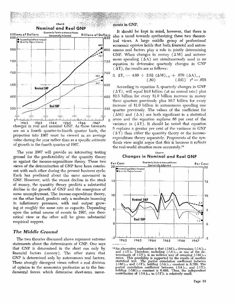
These alternative forecasts can be presented graph-ically. In Chart 3 they are represented as projectedmovements in the level of real and nominal GNP.The preliminary value of nominal GNP for the fourthquarter of 1966 is $759 billion. The quantity theory

would forecast GNP to grow to the level of $787billion by the fourth quarter of 1967. The income-expenditure theory would forecast growth to a level ofabout $805 billion. Similar projections are shown forreal GNP in 1958 prices. In Chart 4 the alternativeforecasts are presented as projections of per cent

laIn the January 10, 1967 State of the Union Message thePresident proposed a 6 per cent surtax on personal and cor-porate income effective July 1, 1967. Even if adopted asproposed, the effect on CNP estimates for 1967 as a wholewould probably be small.

of money through 1966, continuation of the average suiting forecast of GNP will also be poor. But thisrelationship between money and CNP which has does not imply that the theory underlying the fore-existed over the past eight years would imply a cast is necessarily wrong.growth in nominal GNP of about $22 billion (atan annual rate) from the fourth quarter 1966 tothe third quarter 1967. This is about one-half the rateof growth for the same period in 1966. To estimateGNP for all of 1967 requires a prediction of changesin the stock of money during the first quarter of 1967.Money declined about $1 billion in the last half of1966. It has shown little change thus far this yearfrom the average of the fourth quarter of 1966. Ifthis unchanged state continues during the rest of thefirst quarter of 1967, then GNP would increase about$28 billion or 3.7 per cent from the fourth quarter of1966 to the fourth quarter of 1967, or from $759 billionto $787 billion. This is much smaller than the $55billion or 7.8 per cent increase from the fourth quar-ter of 1965 to the fourth quarter of 1966.

S

0

0

Cttorta ments in GNPNominal and Real GNP

I . ouarterfylotafs otannuclkosesB thhto ns of Dollars SeosonoffyAdfusred B’ lhto n $ 0

1 Do liars850 850

L.1962 1963 1964 1965 1966 1967

changes in real and nominal GNP. As these forecastsare on a fourth quarter-to-fourth quarter basis, theprojection into 1967 must be viewed as an averagevalue during the year rather than as a specific estimateof growth in the fourth quarter of 1967.

The year 1967 will provide an interesting testingground for the predictability of the quantity theoryas against the income-expenditure theory. These twoviews of the determination of CMI’ have been consist-ent with each other during the present business cycle.Each has predicted about the same movement inGNP. However, with the recent decline in the stockof money, the quantity theory predicts a substantialdecline in the growth of GNP and the emergence ofsome unemployment. The income-expenditure theory,on the other hand, predicts only a moderate lesseningin inflationary pressures, with real output grow-ing at roughly the same rate as capacity. Dependingupon the actual course of events in 1967, one theo-retical view or the other will be given substantialempirical support.

The two theories discussed above represent extremestatements about the determinants of GNP. One saysthat GNP is determined in the short run only byfinancial factors (money). The other states thatGNP is determined only by autonomous real factors.These strongly divergent views reflect a real divisionof opinion in the economics profession as to the fun-damental forces which determine short-term move-

It should be kept in mind, however, that there isalso a trend towards synthesizing these two theoret-ical views. A large middle group of professionaleconomic opinion holds that both financial and auton-omous real factors play a role in jointly determiningGNP. When changes in money (S M) and autono-mous spending (SA) are simultaneously used in anequation to determine quarterly changes in GNP

SY), the results are as follows:

3. SY, = 4.00 ±2.52 (SM),a + .670 (SA),.,(.80) (.241) r’= .658

According to equation 3, quarterly changes in GNP(S Y) will equal $4.0 billion (at an annual rate) plus$2.5 billion for every $1.0 billion increase in moneythree quarters previously plus $0.7 billion for everyincrease of $1.0 billion in autonomous spending onequarter previously. The values of the coefficient for(SM) and (S A) are both significant in a statistical

0 sense and the equation explains 66 per cent of thevariance in (SY). It should be noted that equation3 explains a greater per cent of the variance in GNP(S Y) than either the quantity theory or the income-expenditure theory separately. Proponents of the syn-thesis view might argue that this is because it reflectsthe real-world situation more accurately.’4

Per Cent

20

15

10

5

0

.5

Chart4

Changes in Nominal and Real GNP

Per Cent

~An alternative explanation is that (L~M)t.,determines (AA)t.sand (L~Y)~.Therefore, including (AA)15 as one of the de-terminants of (u~sY) t is an indirect way of counting (tiM ) t.,

twice, This possibility is supported by the results of anotherstatistical test. The partial correlation coefficient between(tiM)t. and (AY)t holding (AA)r., constant is 0.769. Thepartial correlation coefficient between (tiA )t, and (AY)holding (tiM)t., constant is 0.486. Thus, the independentconfribution of (LxA)u, to (tiY)t is relatively small.

Page 13

800

750

700

650

600

550

• fecome Espetsditure Forecast•Ouontify l’hebrv Foresust

OuarterfyOata atAnnuafRatesSeasonaffv Adiusted

The Middle Ground

1962 1963 1964 1965 1966 1967

The most likely reason for the existence of thedivergent theories described above is that one theo-retical approach or the other may do a superior jOl)of explaining short-term movements in GNP depend-ing upon factors which are not explicitly consideredin either theory. For example, during the 1930sbusiness expectations of the future were so badlyimpaired by the depression experience that evenlarge changes in financial variables like money, bank

The method of testing the respective theories of incomedetermination used here is similar to one originally devisedby Milton Friedman and David Meiselman in an articlepublished in 1963 as “Research Study Two: The RelativeStability of Monetary Velocity and the Investment Mul-tiplier in the United States, 1897-1958” in Stabilization

one of a series of research studies prepared for theCommission on Money and Credit. The purpose of thatstudy was to test empirically the stability of the fundamen-tal behavioral assumptions undetlying each theory. To dothis, they selected definitions of GNP (Y), autonomousspending (A), consumption (C), and money (M) whichseemed to them most appropriate to that task. Since pub-lication of that study there has been much controversywithin the economics professio& regarding the appropri-ateness of using a single-equation model to test competingtheories and also regarding the appropriate definitions ofmajor variables. The purpose of this article is not to testthese theories but only to consider their use as forecastingtools. We have used the definitions of (Y), (A), (C), and(M) which are most widely recognized by the generalpublic although they differ in important respects from thedefinitions used by Friedman and Meiselman,

Each theory is presented as a single-equation model,while the true structure of the economy, and thus the struc-ture of any model which attempts to explain the economy,

is considerably more complicated. However, the use of asingle-equation model of each theory may be justified forseveral reasons. (1) At the theoretical level these single-equation models can he thought of as representing ic-duced forms of a more complex structural model of theeconomy. The intermediate links between the fundamen-tal causal factors (money or autonomous spending) andGNP are netted out. (2) The causal differences betweeneach theory as presented here are sufficiently large (oneemphasizing financial factors and the other real factors)that as a first approximation a very crude single-equationmodel may distinguish between them, (3) As a practicalmatter, an economic model used just for forecasting futureincome can he simpler than a model designed to explainthe structure and interrelationships of the economy.

The measure of aggregate economic activity used hereas a forecasting target is GNP. The use of gross nationalproduct rather than net national product, national income,or disposable income can he criticized for a variety oftheoretical and statistical reasons. The major justificationfor using CNP is that it is the most publicly recognizedaggregate measure of economic activity. It is also the mostwidely forecast value of aggregate economic behavior, andresults obtained here can be compared with other forecasts.If this article were designed to test the theoretical andempirical “correctness” of these tsvo theories (which, itshould be noted, is not the case), then some measure otherthan GNP might have been superior.

This synthesis would not view either monetary or credit availability, and interest rates would not befiscal policy as the dominant tool of Government sufficient to induce new investment and consump-action to the exclusion of the other. Rather, it would tion. In this case, the income-expenditure theory 5consider that there is a possible mix of monetary and would seem to provide a superior explanation offiscal policies which can simultaneously achieve de- short-term movements in CNP. On the other hand,sired levels of income, at other periods when business expectations of the

future are buoyant, as the last five years, the majorrestriction on new investment and consumption is theavailability of money and credit, which would makethe quantity theory a superior explanation. At stillother times, business expectations may be between

these two extremes, in which case a mix or synthesisof the two theories may provide the best explanationof short-term movements of GNP.

MIcHAEL W. KEIIAN

APPENDIX

0

0

1See American Economic Review, September 1965, “The Rela-tive Stability of Monetary Velocity and the Investment Mul-tiplier,” by Albert Ando and Franco Modigliani; “Test of theRelative ltnportance of Autonomous Expenditures and Money,”by Michael DePrano and Thomas Mayer; “Reply to Ando andModigliani and to DePrano and Mayer,u~by Milton Friedmanand David Meiselman. Also see Review of Economics andStatistics, November 1964, “Keynes and The Quantity Theory:a Comment on the Friednian-Meiselman CMC Paper,” byDonald D. Hester, and “Reply to Donald Hester,” by Friedmanand Meiselman.

Page 14

A related problem is the treatment of imports and taxesin the analysis. Although neither of these items appearsexplicitly, both are included implicitly and their inclusioncomplicates the distinction between autonomous and in-duced spending.

The value of GNP in the national income accounts doesnot include taxes directly. Imports, however, are nettedagainst exports. That is, GNP is defined as

1. Y = C + Ig + G + (X — Im)

Y = GNPC = Consumption

Ig = Cross business investment

C = Government spending

X = Exports

Im = Imports

It is necessary to define induced and antonomous spendingin such a way that their sum will equal GNP (Y). Consider-ing these problems, induced spending (I) and autonomousspending (A) have been defined as follows:

2. I = C3. A = Ig + C + (X — Im)2

This problem of adjusting the values of (I) and (A) tomake them consistent with (Y) will arise no matter whatdefinition of income is used. Because this adjusting processis rather arbitrary, reasonable men could disagree with thespecific adjustments used. The rationale for the adjust-ments made here are givenin the two following paragraphs.

Imports are already included in the recorded value ofconsumption, investment, and government spending.Thus, the major behavioral role of imports broken downaccording to its induced and autonomous components isalready included in other values. The value of (I) is notbiased by excluding imports. However, by netting all im-ports against (A) we are introducing some element of in-duced spending which makes this measure of (A) lessaccurate than would be ideal, although its quantitativeimportance is not likely to be large.

2Some very minor additional items which are part of CNPare included in A.

Another important issue with respect to the income-expenditure theory has to do with the fact that (A) is notonly the theoretical determinant of (Y) but also an account-ing component of (Y). That is:

Or

And

4. Y = I + A [Accounting definitionl

4a. AY = AT + AA

5. Ay = a + b(AA) [Theoretical assumptionl

Any statistical test of the theoretical relation between (AA)and (AY) would give a much closer link between the twovariables than would actually be the case, because in anaccounting sense (AA) is included in (AY). This problemhas been handled by relating (AA) to (AY) with a one-quarter time lag which breaks the link with the accountingdefinition. An alternative and perhaps conceptually supe-rior method would be to compare (AA) only with thosecomponents of (AY) which are not included in (A A).Because (AY AA = AT) this would mean comparing(IsA) with (Al). If

6. Al = c + d(AY) [Because induced spending (I)depends upon current income(Y).l

ThenAJ = c + d(AI) + d(AA) [Because(Y)canbe

written as (I + A).l

Al (1 ~—d) = c + d(AA) [Collecting all (I) terms

on the left-hand side.l

c d [Dividing both sides

7. Al = + 1—~-(AA) by (1-d).l

Thus, (Al) depends upon (IsA).

When this relation is tested statistically, the results areas follows:

7a. AJ = 3.42 + .550 (AA)t5 r2 .372

(.133)

These results are statistically significant and almost as goodas equation 2a in the text which relates (A) to (Y)

Page 15

/

There has been relatively little contmversy among pro- To the extent that rates are unchanged, taxes are de-fessional economists about the procedures for testing the pendent upon changes in income, and their effect is thereby

P significance of the quantity theory, with the possible ex- reflected in consumption (C). However, changes in taxception of discussion of the appropriate definition of money rates are an important discretionary tool of fiscal policy,(see footnotes 6 and 10 in the text). However, with respect Therefore some measure of their effect on consumptionto the income-expenditure theory, a major problem is the (C) should be included in autonomous spending (A). Asmethod of specifying what is autonomous spending and a practical matter, there is no simple, clear-cut way towhat is induced spending. It is difficult, if not impossible, separate these two components of taxes. To the extent thatto distinguish statistically which components of income arc important changes in tax structure take place, the measureinduced and which coTnponents are autonomous. Some of (A) is weakened, at least in the time periods during,elements in personal consumption, like durable goods, are and just after, the change in the tax structure. There wasonly weakly related to current income. On the other hand, an important change in the tax structure in 1964 whichsome part of business investment is induced by changes in makes the observed relation between (A) and (Y) or (C)current income. In this article all consumption is consid- weaker than was really the case, l-Iowever, no majorered induced and all investment is considered autonomous, change in the tax structure is likely for 1967 so the use of

(A) in forecasting 1967 will not be seriously impaired.

It is interesting to note that when changes in money arc Friedman and Meiselman observed this superior relationc mpared with changes in induced spending only the in their study and attributed it to the fact that money shouldresults are actually superior to money related to CNP. he related to permanent (rather than observed) income 0

8. LIt 3~ 4 2]3 (AM) t. r~- 5J1 and that consumption or induced spending is superior to.:3~) (1) as a proxy for permanent incori IC.

Page 16