have economic models' forecasting performance for … · have economic models’ forecasting...
TRANSCRIPT
Have Economic Models’ Forecasting Performance for US Output
Growth and Inflation Changed Over Time, and When?
Not-For-Publication Appendix ∗
Barbara Rossi and Tatevik Sekhposyan
Duke University UNC - Chapel Hill
First draft: July 2007. This revision: July 2009.
General comments
1. Data sources for the revised data are provided in Table 1. Real time employment and indus-
trial production index are the monthly vintages of Nonfarm Payroll Employment (EMPLOY)
and Total Industrial Production Index (IPT) series provided by the Federal Reserve Bank of
Philadelphia Real-Time Data Set (http://www.philadelphiafed.org/econ/forecast/real-time-
data/data-files/). The monthly vintages of the Civilian Unemployment Rate (UNRATE) are
from the ArchivaL Federal Reserve Economic Data (ALFRED) database of the St. Louis
Fed.
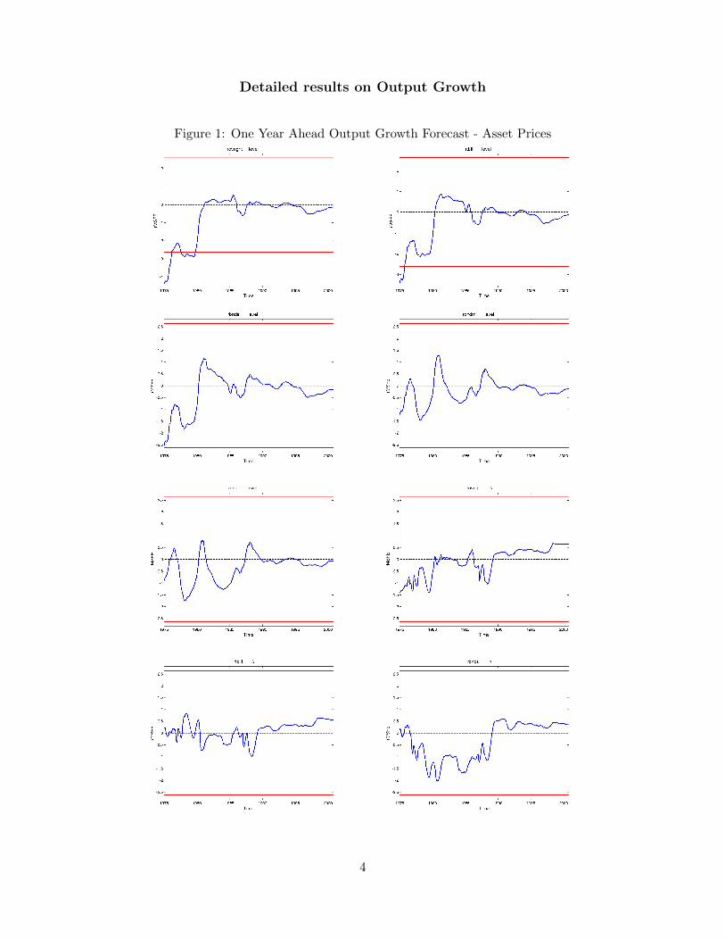
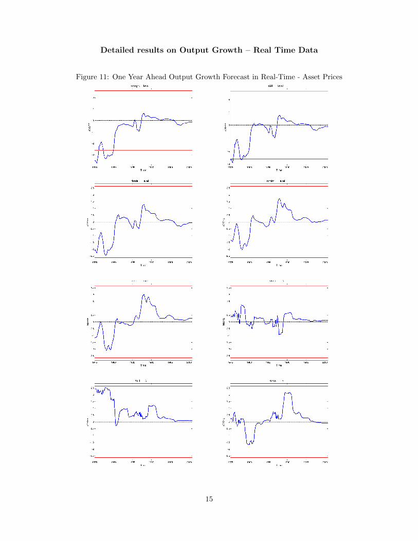
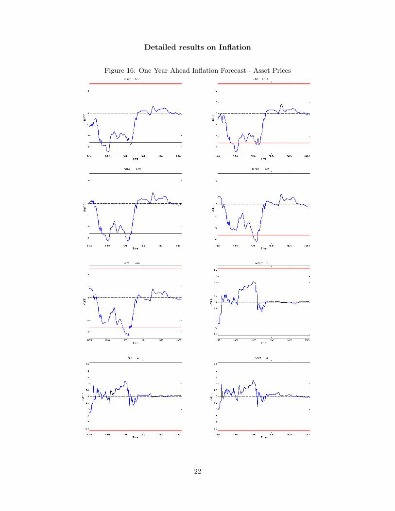
2. Notes to the figures: The dark solid line in the figure reports the re-scaled rMSFEs, that
is FOOSt,m = σ̂−1m−1/2rMSFEt. The light solid lines report 90% bands for testing the null
hypothesis that the models’ relative forecasting performance is equal (the test rejects when
the dark solid line is outside the bands). Negative values of the re-scaled rMSFE denote
situations in which the economic model forecasts better than its competitor. For details,
refer to the paper.
∗This appendix reports the additional results for Rossi, B. & Sekhposyan, T. (2010). Have Economic Models’Forecasting Performance for US Output Growth and Inflation Changed Over Time, and When? International Journalof Forecasting 26(4), 2010, 808-835.
1
Table 1: Description of Data Series
Label Period Name Description S
Asset Prices
rovnght 1959:1 - 2005:12 FYFF Int Rate: Federal Funds (Effective) D
rtbill 1959:1 - 2005:12 FYGM3 Int Rate: US Treasury Bills, Sec Mkt, 3-Mo D
rbnds 1959:1 - 2005:12 FYGT1 Int Rate: US Treasury Const Maturities, 1-Yr D
rbndm 1959:1 - 2005:12 FYGT5 Int Rate: US Treasury Const Maturities, 5-Yr D
rbndl 1959:1 - 2005:12 FYGT10 Int Rate: US Treasury Const Maturities, 10-Yr D
exrate 1959:1 - 2005:12 EXRUS United States; Effective Exchange Rate D
stockp 1959:1 - 2005:12 FSPCOM S&P’s Common Stock Price Index: Composite D
Activity
ip 1959:1 - 2005:12 B5001 Industrial Production Total (sa) F
capu 1959:1 - 2002:06 IPXMCA Capacity Utilization Rate: MFG, Total D
emp 1959:1 - 2005:12 LHEM Civilian Labor Force: Employed, Total D
unemp 1959:1 - 2005:12 LHUR Unemp Rate: All Workers, 16 Years and Over D
hours 1959:1 - 2005:12 A0M001 Average weekly hours, mfg. (hours) C
deliveries 1959:1 - 2005:12 A0M032 Index of supplier deliveries - vendor perf. (pct.) C
Wages and Prices
cpi 1959:1 - 2005:12 CUUR0000AA0 CPI - All Urban Consumers (nsa) B
pce 1959:1 - 2005:12 PCE deflator Price Indexes for Personal Cons. Expenditures B
ppi 1959:1 - 2005:12 PW Producer Price Index: All Commodities D
earn 1959:1 - 2003:04 LE6GP Avg Hourly Earnings - Goods - Producing D
oil 1959:1 - 2003:06 WPU0561 Crude Petroleum (Domestic Production) B
Money
m0 1959:1 - 2003:06 FMBASE Monetary Base, Adj For Reserve Req Chgs D
m1 1959:1 - 2005:12 FM1 Money Stock: M1 D
m2 1959:1 - 2005:12 FM2 Money Stock: M2 D
m3 1959:1 - 2005:12 FM3 Money Stock: M3 D
Miscellaneous
lead 1959:1 - 2005:12 G0M910 Composite index of 10 leading indicators C
Note: Sources (S) are abbreviated as follows: B - Bureau of Labor Statistics, C - Conference Board, D -
DRI Basic Economics Database, F - Federal Reserve Board of Governors. S pread is defined as the difference
between rbndl and rovnght. The same names preceded by an “r” denote the real version of the variable.
For example, Real Interest Rates (such as rrovnght, rrtbill, rrbnds, rrbndm, rrbndl) are defined as Nominal
Interest Rates minus CPI inflation. Real stock variables such as Real Money Balances (rm0, rm1, rm2, rm3)
are defined as the ratio of the Nominal Money Balances and CPI.
2

Section 1: Detailed results for all available series
3
Detailed results on Output Growth
Figure 1: One Year Ahead Output Growth Forecast - Asset Prices
4
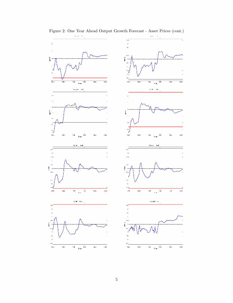
Figure 2: One Year Ahead Output Growth Forecast - Asset Prices (cont.)
5
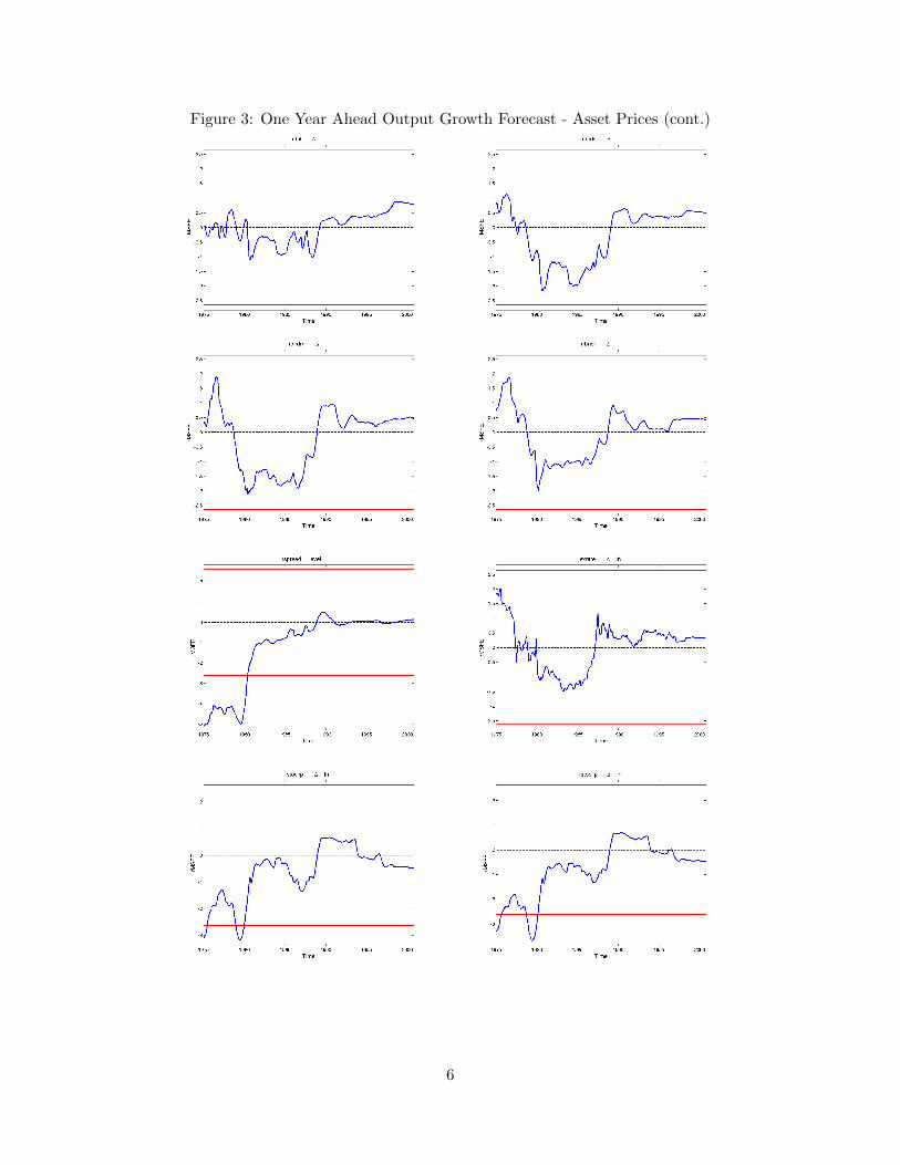
Figure 3: One Year Ahead Output Growth Forecast - Asset Prices (cont.)
6
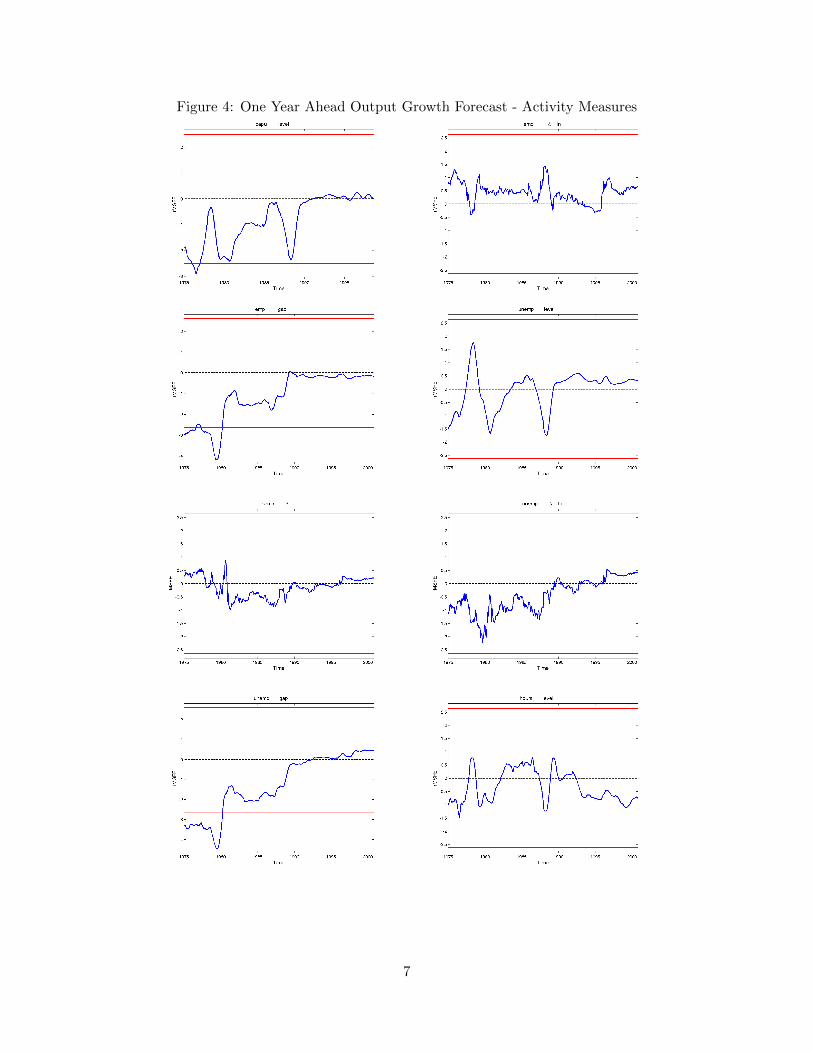
Figure 4: One Year Ahead Output Growth Forecast - Activity Measures
7
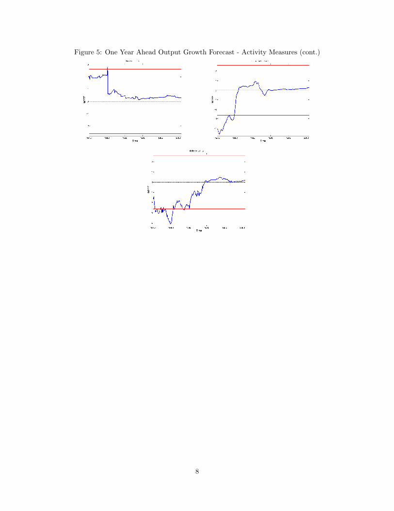
Figure 5: One Year Ahead Output Growth Forecast - Activity Measures (cont.)
8
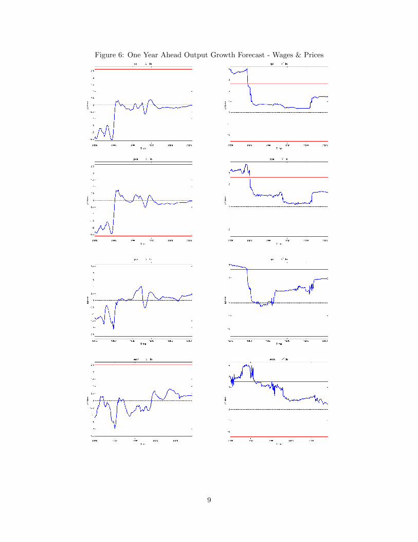
Figure 6: One Year Ahead Output Growth Forecast - Wages & Prices
9
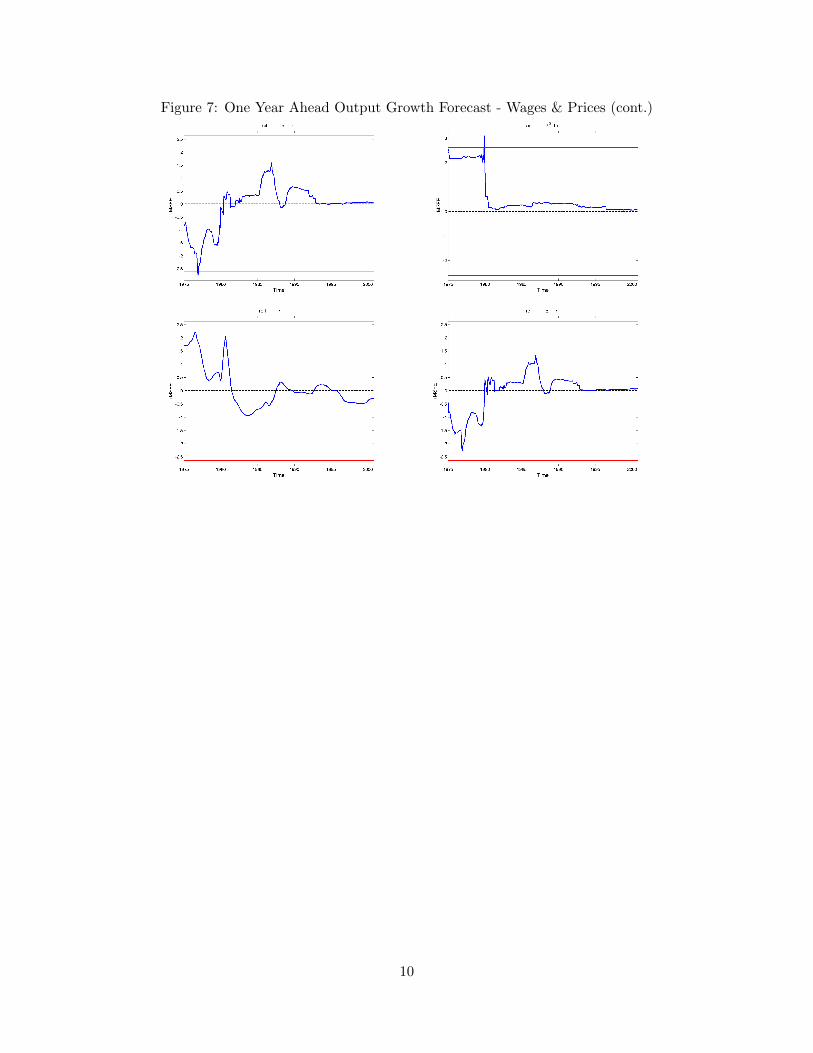
Figure 7: One Year Ahead Output Growth Forecast - Wages & Prices (cont.)
10
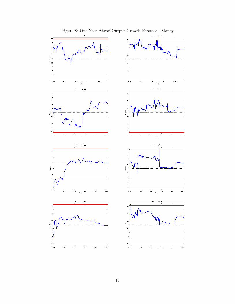
Figure 8: One Year Ahead Output Growth Forecast - Money
11
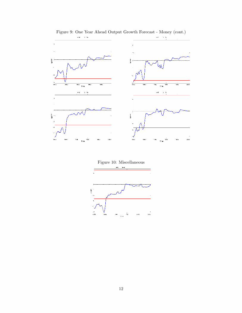
Figure 9: One Year Ahead Output Growth Forecast - Money (cont.)
Figure 10: Miscellaneous
12
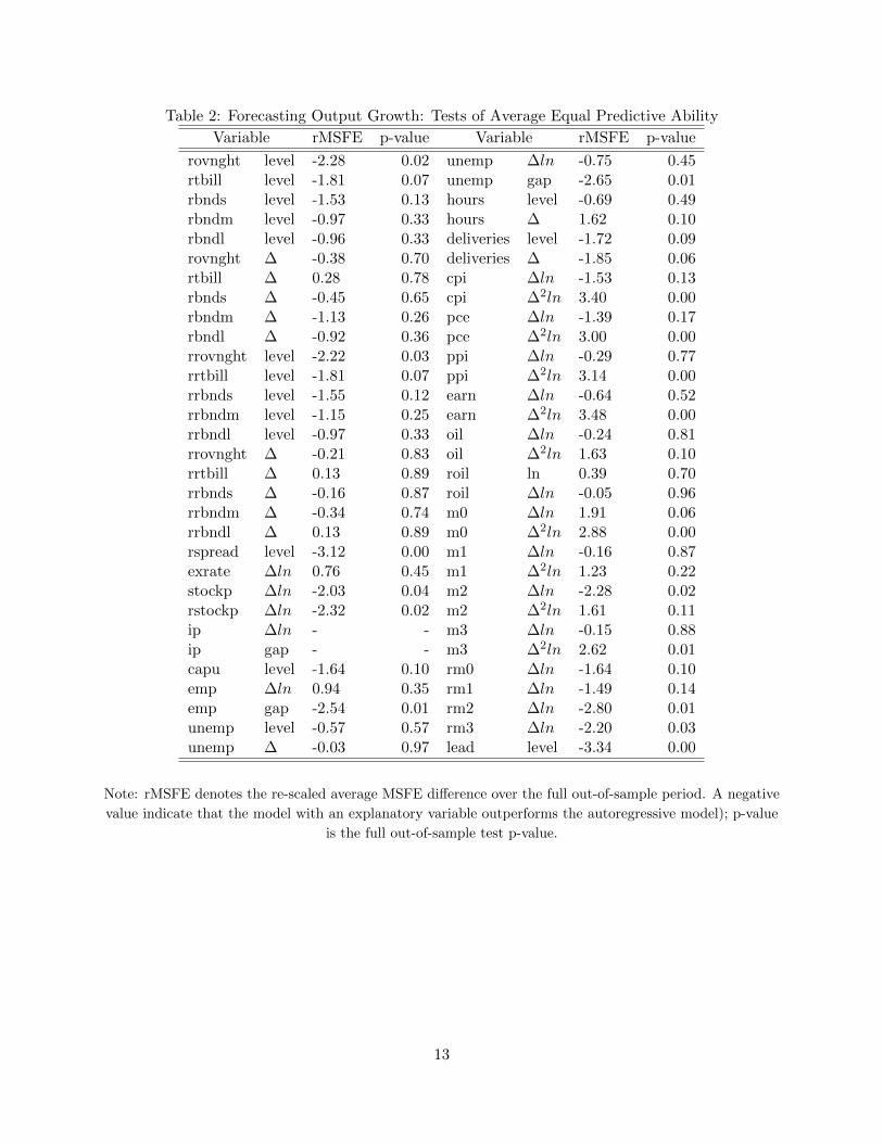
Table 2: Forecasting Output Growth: Tests of Average Equal Predictive Ability
Variable rMSFE p-value Variable rMSFE p-value
rovnght level -2.28 0.02 unemp ∆ln -0.75 0.45rtbill level -1.81 0.07 unemp gap -2.65 0.01rbnds level -1.53 0.13 hours level -0.69 0.49rbndm level -0.97 0.33 hours ∆ 1.62 0.10rbndl level -0.96 0.33 deliveries level -1.72 0.09rovnght ∆ -0.38 0.70 deliveries ∆ -1.85 0.06rtbill ∆ 0.28 0.78 cpi ∆ln -1.53 0.13rbnds ∆ -0.45 0.65 cpi ∆2ln 3.40 0.00rbndm ∆ -1.13 0.26 pce ∆ln -1.39 0.17rbndl ∆ -0.92 0.36 pce ∆2ln 3.00 0.00rrovnght level -2.22 0.03 ppi ∆ln -0.29 0.77rrtbill level -1.81 0.07 ppi ∆2ln 3.14 0.00rrbnds level -1.55 0.12 earn ∆ln -0.64 0.52rrbndm level -1.15 0.25 earn ∆2ln 3.48 0.00rrbndl level -0.97 0.33 oil ∆ln -0.24 0.81rrovnght ∆ -0.21 0.83 oil ∆2ln 1.63 0.10rrtbill ∆ 0.13 0.89 roil ln 0.39 0.70rrbnds ∆ -0.16 0.87 roil ∆ln -0.05 0.96rrbndm ∆ -0.34 0.74 m0 ∆ln 1.91 0.06rrbndl ∆ 0.13 0.89 m0 ∆2ln 2.88 0.00rspread level -3.12 0.00 m1 ∆ln -0.16 0.87exrate ∆ln 0.76 0.45 m1 ∆2ln 1.23 0.22stockp ∆ln -2.03 0.04 m2 ∆ln -2.28 0.02rstockp ∆ln -2.32 0.02 m2 ∆2ln 1.61 0.11ip ∆ln - - m3 ∆ln -0.15 0.88ip gap - - m3 ∆2ln 2.62 0.01capu level -1.64 0.10 rm0 ∆ln -1.64 0.10emp ∆ln 0.94 0.35 rm1 ∆ln -1.49 0.14emp gap -2.54 0.01 rm2 ∆ln -2.80 0.01unemp level -0.57 0.57 rm3 ∆ln -2.20 0.03unemp ∆ -0.03 0.97 lead level -3.34 0.00
Note: rMSFE denotes the re-scaled average MSFE difference over the full out-of-sample period. A negative
value indicate that the model with an explanatory variable outperforms the autoregressive model); p-value
is the full out-of-sample test p-value.
13
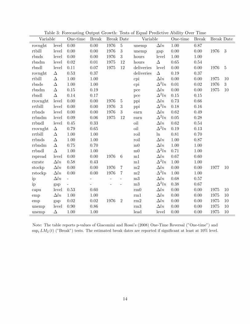
Table 3: Forecasting Output Growth: Tests of Equal Predictive Ability Over Time
Variable One-time Break Break Date Variable One-time Break Break Date
rovnght level 0.00 0.00 1976 5 unemp ∆ln 1.00 0.87rtbill level 0.00 0.00 1976 3 unemp gap 0.00 0.00 1976 3rbnds level 0.00 0.00 1976 3 hours level 1.00 1.00rbndm level 0.02 0.01 1975 12 hours ∆ 0.65 0.54rbndl level 0.11 0.07 1975 12 deliveries level 0.00 0.00 1976 5rovnght ∆ 0.53 0.37 deliveries ∆ 0.19 0.37rtbill ∆ 1.00 1.00 cpi ∆ln 0.00 0.00 1975 10rbnds ∆ 1.00 1.00 cpi ∆2ln 0.01 0.02 1976 3rbndm ∆ 0.15 0.19 pce ∆ln 0.00 0.00 1975 10rbndl ∆ 0.14 0.17 pce ∆2ln 0.15 0.15rrovnght level 0.00 0.00 1976 5 ppi ∆ln 0.73 0.66rrtbill level 0.00 0.00 1976 3 ppi ∆2ln 0.18 0.16rrbnds level 0.00 0.00 1976 3 earn ∆ln 0.62 0.49rrbndm level 0.09 0.06 1975 12 earn ∆2ln 0.05 0.28rrbndl level 0.45 0.33 oil ∆ln 0.62 0.54rrovnght ∆ 0.79 0.65 oil ∆2ln 0.19 0.13rrtbill ∆ 1.00 1.00 roil ln 0.81 0.70rrbnds ∆ 1.00 1.00 roil ∆ln 1.00 0.87rrbndm ∆ 0.75 0.70 m0 ∆ln 1.00 1.00rrbndl ∆ 1.00 1.00 m0 ∆2ln 0.71 1.00rspread level 0.00 0.00 1976 6 m1 ∆ln 0.67 0.60exrate ∆ln 0.58 0.43 m1 ∆2ln 1.00 1.00stockp ∆ln 0.00 0.00 1976 7 m2 ∆ln 0.00 0.00 1977 10rstockp ∆ln 0.00 0.00 1976 7 m2 ∆2ln 1.00 1.00ip ∆ln - - - - m3 ∆ln 0.68 0.57ip gap - - - - m3 ∆2ln 0.38 0.67capu level 0.53 0.60 rm0 ∆ln 0.00 0.00 1975 10emp ∆ln 1.00 1.00 rm1 ∆ln 0.00 0.00 1975 10emp gap 0.02 0.02 1976 2 rm2 ∆ln 0.00 0.00 1975 10unemp level 0.90 0.86 rm3 ∆ln 0.00 0.00 1975 10unemp ∆ 1.00 1.00 lead level 0.00 0.00 1975 10
Note: The table reports p-values of Giacomini and Rossi’s (2008) One-Time Reversal (”One-time”) and
supt LM2 (t) (”Break”) tests. The estimated break dates are reported if significant at least at 10% level.
14
Detailed results on Output Growth – Real Time Data
Figure 11: One Year Ahead Output Growth Forecast in Real-Time - Asset Prices
15
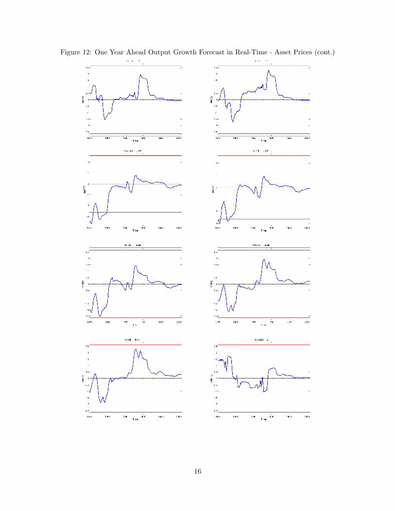
Figure 12: One Year Ahead Output Growth Forecast in Real-Time - Asset Prices (cont.)
16
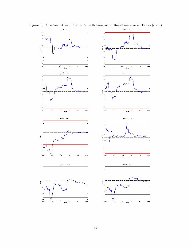
Figure 13: One Year Ahead Output Growth Forecast in Real-Time - Asset Prices (cont.)
17
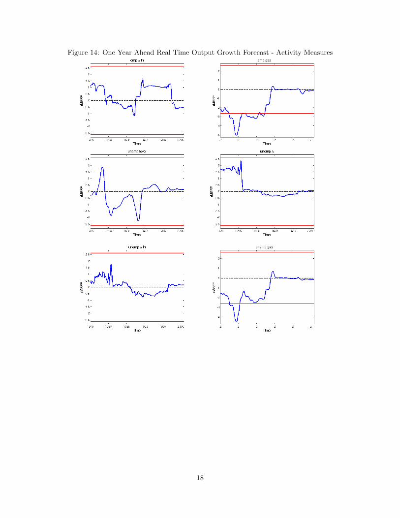
Figure 14: One Year Ahead Real Time Output Growth Forecast - Activity Measures
18

Figure 15: One Year Ahead Real Time Output Growth Forecast - Prices
19

Table 4: Forecasting Output Growth in Real-Time: Tests of Average Equal Predictive Ability
Variable rMSFE p-value Variable rMSFE p-value
rovnght level -2.14 0.03 rrtbill ∆ 1.30 0.19rtbill level -1.72 0.08 rrbnds ∆ 0.36 0.72rbnds level -1.30 0.19 rrbndm ∆ 0.55 0.58rbndm level -0.66 0.51 rrbndl ∆ 0.83 0.41rbndl level -0.44 0.66 rspread level -2.60 0.01rovnght ∆ 0.26 0.79 exrate ∆ln 1.04 0.30rtbill ∆ 1.67 0.10 stockp ∆ln -1.66 0.10rbnds ∆ 0.30 0.76 rstockp ∆ln -1.91 0.06rbndm ∆ 0.35 0.73 emp ∆ln 0.50 0.62rbndl ∆ 0.39 0.70 emp gap -2.92 0.00rrovnght level -2.03 0.04 unemp level -0.50 0.62rrtbill level -1.73 0.08 unemp ∆ 0.85 0.39rrbnds level -1.28 0.20 unemp ∆ln 0.23 0.82rrbndm level -0.64 0.52 unemp gap -2.23 0.03rrbndl level -0.22 0.83 cpi ∆ln -1.38 0.17rrovnght ∆ 0.51 0.61 cpi ∆2ln 0.98 0.33
Note: rMSFE denotes the re-scaled average MSFE difference over the full out-of-sample period. A negative
value indicate that the model with an explanatory variable outperforms the autoregressive model); p-value
is the full out-of-sample test p-value.
20
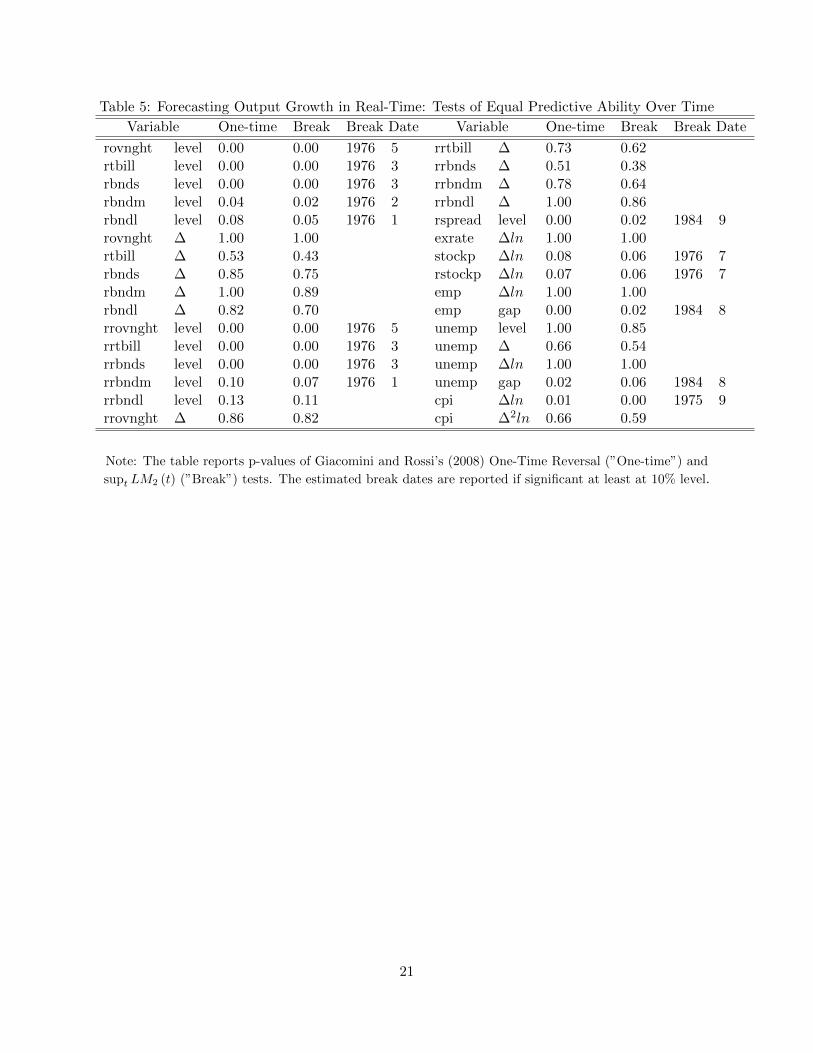
Table 5: Forecasting Output Growth in Real-Time: Tests of Equal Predictive Ability Over Time
Variable One-time Break Break Date Variable One-time Break Break Date
rovnght level 0.00 0.00 1976 5 rrtbill ∆ 0.73 0.62rtbill level 0.00 0.00 1976 3 rrbnds ∆ 0.51 0.38rbnds level 0.00 0.00 1976 3 rrbndm ∆ 0.78 0.64rbndm level 0.04 0.02 1976 2 rrbndl ∆ 1.00 0.86rbndl level 0.08 0.05 1976 1 rspread level 0.00 0.02 1984 9rovnght ∆ 1.00 1.00 exrate ∆ln 1.00 1.00rtbill ∆ 0.53 0.43 stockp ∆ln 0.08 0.06 1976 7rbnds ∆ 0.85 0.75 rstockp ∆ln 0.07 0.06 1976 7rbndm ∆ 1.00 0.89 emp ∆ln 1.00 1.00rbndl ∆ 0.82 0.70 emp gap 0.00 0.02 1984 8rrovnght level 0.00 0.00 1976 5 unemp level 1.00 0.85rrtbill level 0.00 0.00 1976 3 unemp ∆ 0.66 0.54rrbnds level 0.00 0.00 1976 3 unemp ∆ln 1.00 1.00rrbndm level 0.10 0.07 1976 1 unemp gap 0.02 0.06 1984 8rrbndl level 0.13 0.11 cpi ∆ln 0.01 0.00 1975 9rrovnght ∆ 0.86 0.82 cpi ∆2ln 0.66 0.59
Note: The table reports p-values of Giacomini and Rossi’s (2008) One-Time Reversal (”One-time”) and
supt LM2 (t) (”Break”) tests. The estimated break dates are reported if significant at least at 10% level.
21
Detailed results on Inflation
Figure 16: One Year Ahead Inflation Forecast - Asset Prices
22
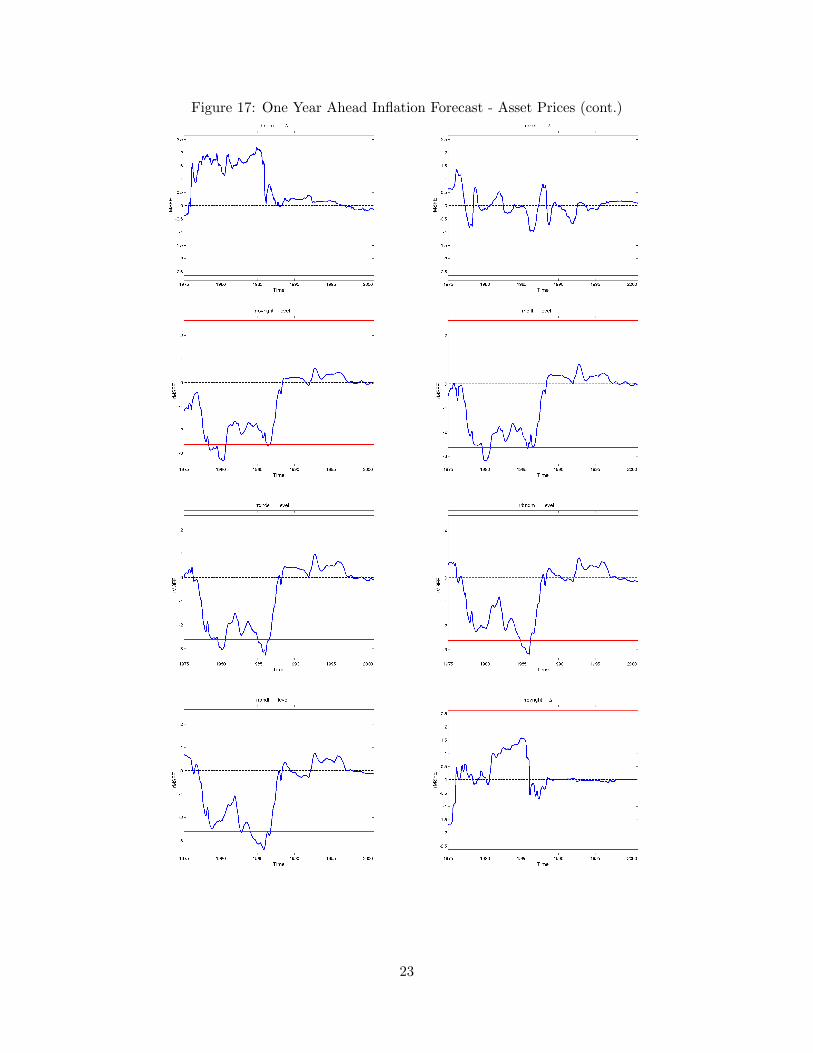
Figure 17: One Year Ahead Inflation Forecast - Asset Prices (cont.)
23
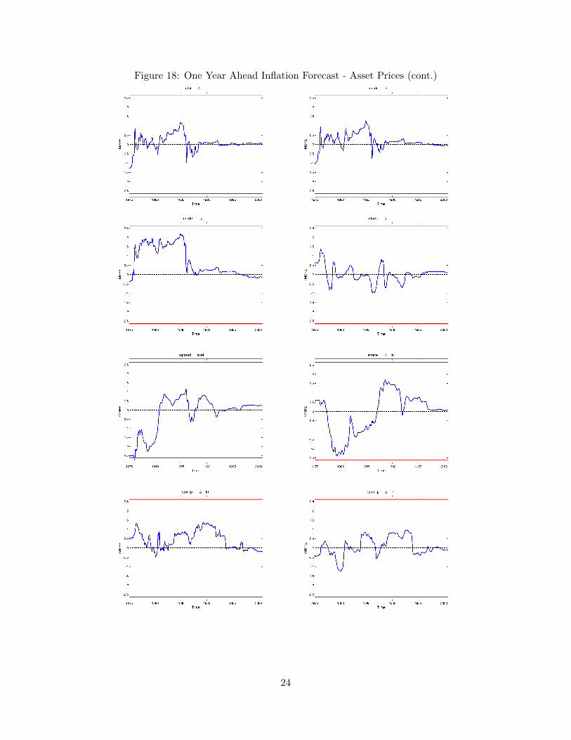
Figure 18: One Year Ahead Inflation Forecast - Asset Prices (cont.)
24
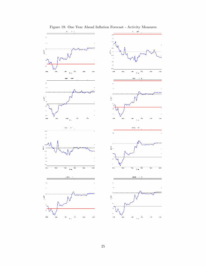
Figure 19: One Year Ahead Inflation Forecast - Activity Measures
25
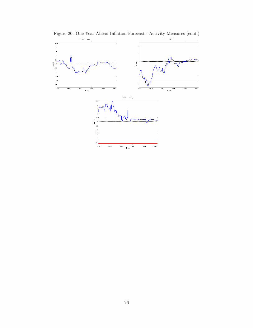
Figure 20: One Year Ahead Inflation Forecast - Activity Measures (cont.)
26
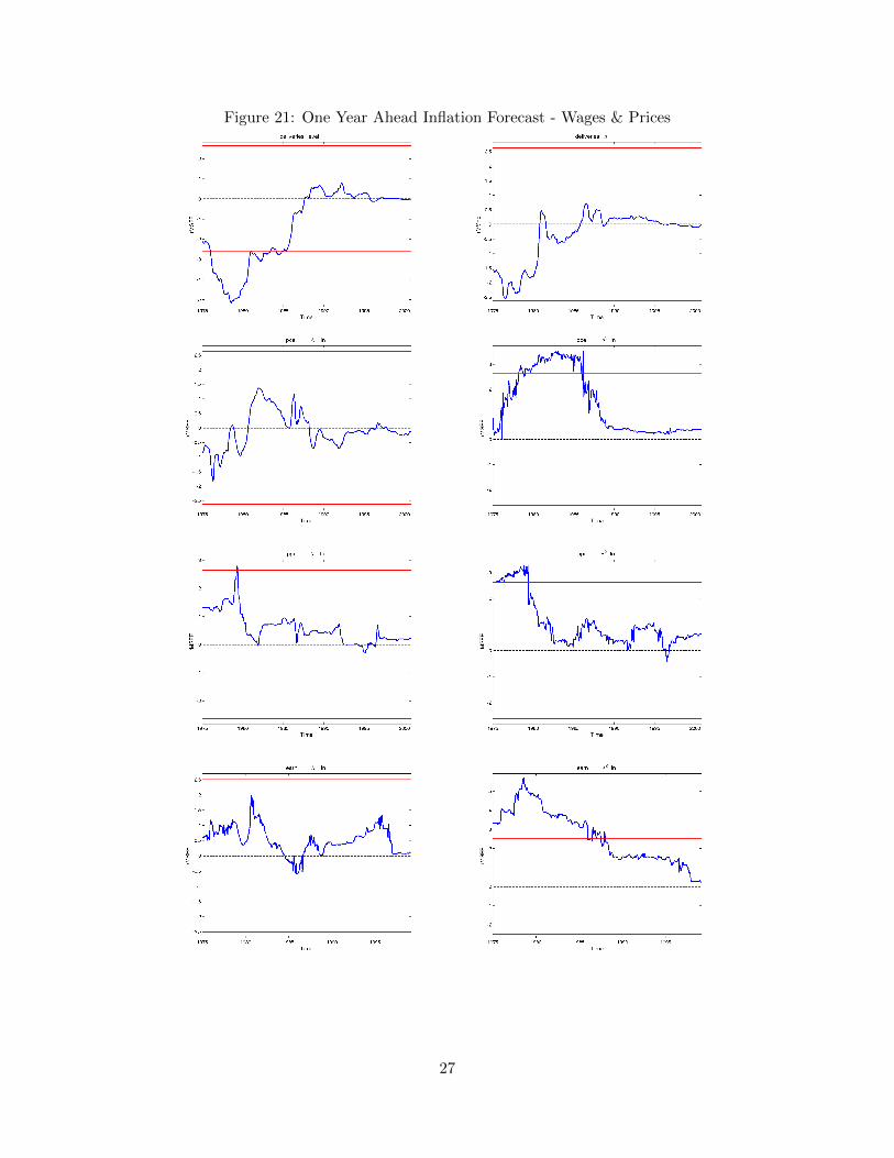
Figure 21: One Year Ahead Inflation Forecast - Wages & Prices
27
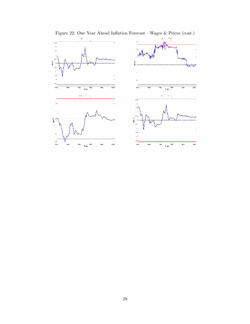
Figure 22: One Year Ahead Inflation Forecast - Wages & Prices (cont.)
28
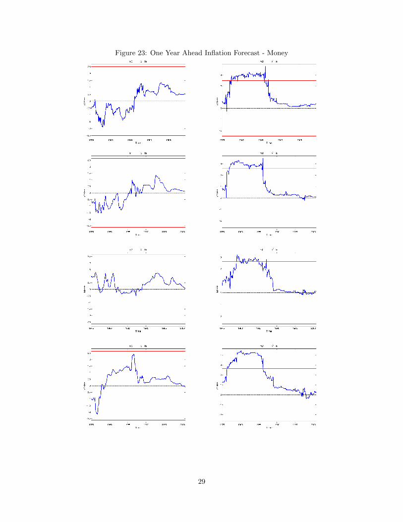
Figure 23: One Year Ahead Inflation Forecast - Money
29
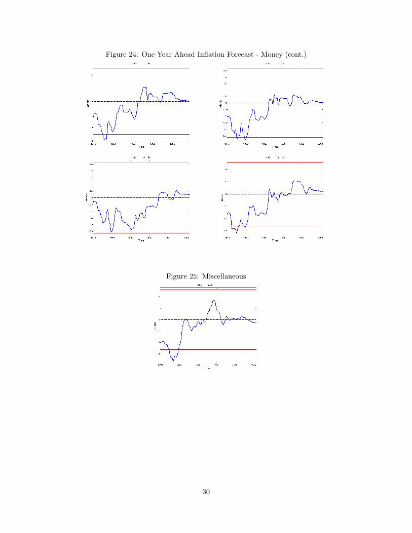
Figure 24: One Year Ahead Inflation Forecast - Money (cont.)
Figure 25: Miscellaneous
30
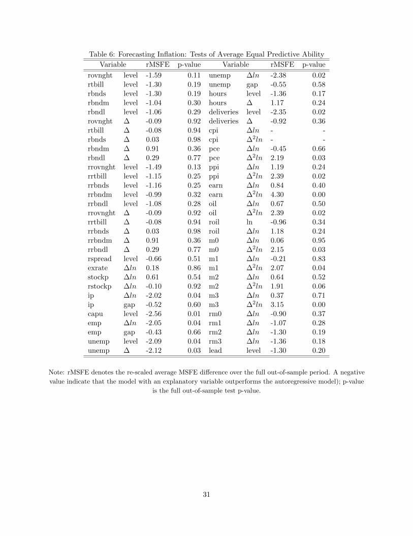
Table 6: Forecasting Inflation: Tests of Average Equal Predictive Ability
Variable rMSFE p-value Variable rMSFE p-value
rovnght level -1.59 0.11 unemp ∆ln -2.38 0.02rtbill level -1.30 0.19 unemp gap -0.55 0.58rbnds level -1.30 0.19 hours level -1.36 0.17rbndm level -1.04 0.30 hours ∆ 1.17 0.24rbndl level -1.06 0.29 deliveries level -2.35 0.02rovnght ∆ -0.09 0.92 deliveries ∆ -0.92 0.36rtbill ∆ -0.08 0.94 cpi ∆ln - -rbnds ∆ 0.03 0.98 cpi ∆2ln - -rbndm ∆ 0.91 0.36 pce ∆ln -0.45 0.66rbndl ∆ 0.29 0.77 pce ∆2ln 2.19 0.03rrovnght level -1.49 0.13 ppi ∆ln 1.19 0.24rrtbill level -1.15 0.25 ppi ∆2ln 2.39 0.02rrbnds level -1.16 0.25 earn ∆ln 0.84 0.40rrbndm level -0.99 0.32 earn ∆2ln 4.30 0.00rrbndl level -1.08 0.28 oil ∆ln 0.67 0.50rrovnght ∆ -0.09 0.92 oil ∆2ln 2.39 0.02rrtbill ∆ -0.08 0.94 roil ln -0.96 0.34rrbnds ∆ 0.03 0.98 roil ∆ln 1.18 0.24rrbndm ∆ 0.91 0.36 m0 ∆ln 0.06 0.95rrbndl ∆ 0.29 0.77 m0 ∆2ln 2.15 0.03rspread level -0.66 0.51 m1 ∆ln -0.21 0.83exrate ∆ln 0.18 0.86 m1 ∆2ln 2.07 0.04stockp ∆ln 0.61 0.54 m2 ∆ln 0.64 0.52rstockp ∆ln -0.10 0.92 m2 ∆2ln 1.91 0.06ip ∆ln -2.02 0.04 m3 ∆ln 0.37 0.71ip gap -0.52 0.60 m3 ∆2ln 3.15 0.00capu level -2.56 0.01 rm0 ∆ln -0.90 0.37emp ∆ln -2.05 0.04 rm1 ∆ln -1.07 0.28emp gap -0.43 0.66 rm2 ∆ln -1.30 0.19unemp level -2.09 0.04 rm3 ∆ln -1.36 0.18unemp ∆ -2.12 0.03 lead level -1.30 0.20
Note: rMSFE denotes the re-scaled average MSFE difference over the full out-of-sample period. A negative
value indicate that the model with an explanatory variable outperforms the autoregressive model); p-value
is the full out-of-sample test p-value.
31

Table 7: Forecasting Inflation: Tests of Equal Predictive Ability Over Time
Variable One-time Break Break Date Variable One-time Break Break Date
rovnght level 0.39 0.57 unemp ∆ln 0.00 0.03 1984 8rtbill level 0.50 0.63 unemp gap 0.79 0.67rbnds level 0.42 0.55 hours level 0.14 0.19rbndm level 0.73 0.80 hours ∆ 1.00 1.00rbndl level 0.76 0.83 deliveries level 0.00 0.02 1983 8rovnght ∆ 0.80 0.70 deliveries ∆ 0.16 0.11rtbill ∆ 1.00 1.00 cpi ∆ln - - - -rbnds ∆ 1.00 1.00 cpi ∆2ln - - - -rbndm ∆ 1.00 1.00 pce ∆ln 0.83 0.78rbndl ∆ 1.00 1.00 pce ∆2ln 0.58 0.78rrovnght level 0.45 0.62 ppi ∆ln 1.00 1.00rrtbill level 0.60 0.70 ppi ∆2ln 0.31 0.26rrbnds level 0.51 0.61 earn ∆ln 1.00 0.83rrbndm level 0.79 0.84 earn ∆2ln 0.00 0.07 1983 9rrbndl level 0.76 0.83 oil ∆ln 1.00 0.83rrovnght ∆ 0.80 0.70 oil ∆2ln 0.18 0.60rrtbill ∆ 1.00 1.00 roil ln 0.47 0.48rrbnds ∆ 1.00 1.00 roil ∆ln 0.51 0.38rrbndm ∆ 1.00 1.00 m0 ∆ln 0.80 0.70rrbndl ∆ 1.00 1.00 m0 ∆2ln 0.65 0.80rspread level 0.28 0.19 m1 ∆ln 1.00 0.88exrate ∆ln 1.00 0.83 m1 ∆2ln 0.37 0.57stockp ∆ln 1.00 1.00 m2 ∆ln 1.00 1.00rstockp ∆ln 0.89 0.79 m2 ∆2ln 0.48 0.64ip ∆ln 0.10 0.20 m3 ∆ln 0.40 0.28ip gap 0.82 0.69 m3 ∆2ln 0.06 0.26capu level 0.00 0.00 1983 10 rm0 ∆ln 0.32 0.34emp ∆ln 0.00 0.03 1983 10 rm1 ∆ln 0.46 0.47emp gap 0.82 0.70 rm2 ∆ln 0.70 0.86unemp level 0.00 0.04 1983 10 rm3 ∆ln 0.29 0.31unemp ∆ 0.03 0.08 1984 7 lead level 0.04 0.06 1984 6
Note: The table reports p-values of Giacomini and Rossi’s (2008) One-Time Reversal (”One-time”) and
supt LM2 (t) (”Break”) tests. The estimated break dates are reported if significant at least at 10% level.
32

Section 2: Robustness to recursive BIC lag length selection
33
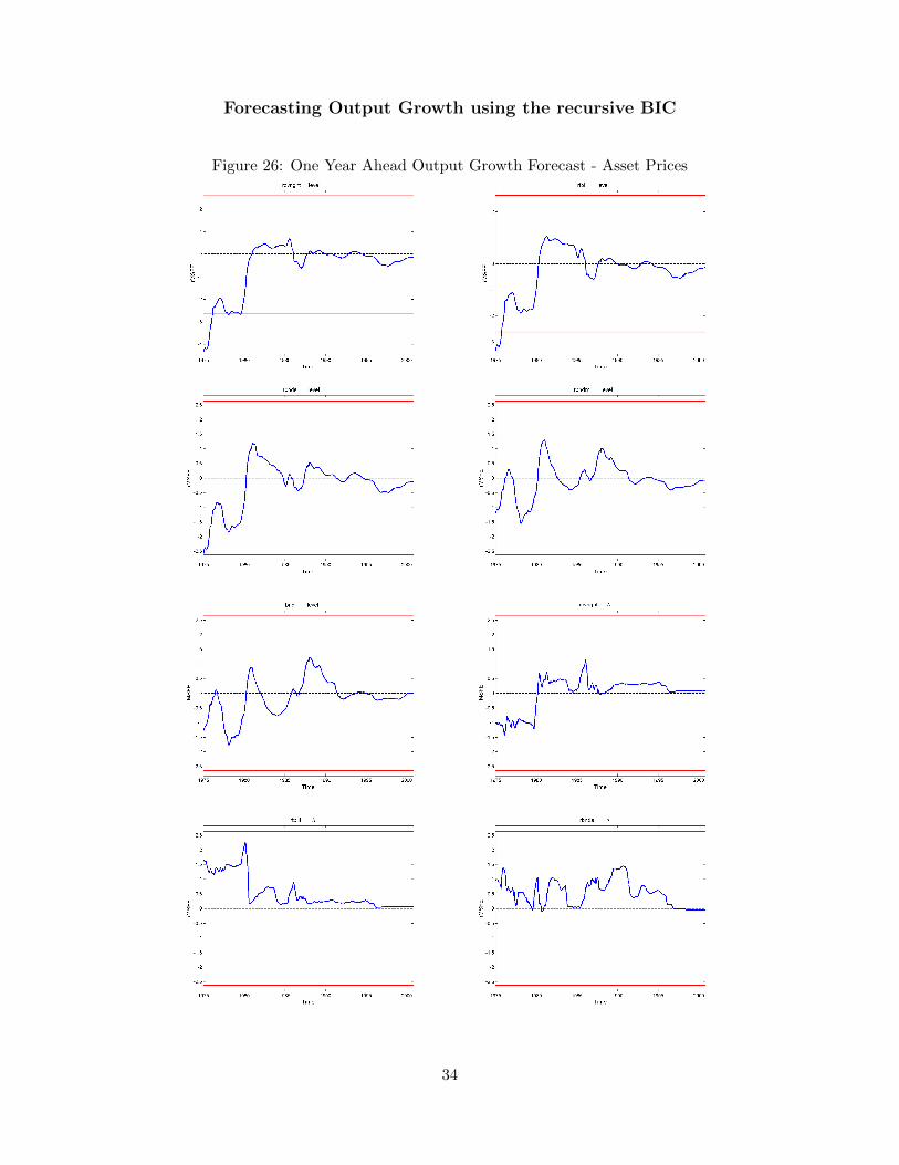
Forecasting Output Growth using the recursive BIC
Figure 26: One Year Ahead Output Growth Forecast - Asset Prices
34
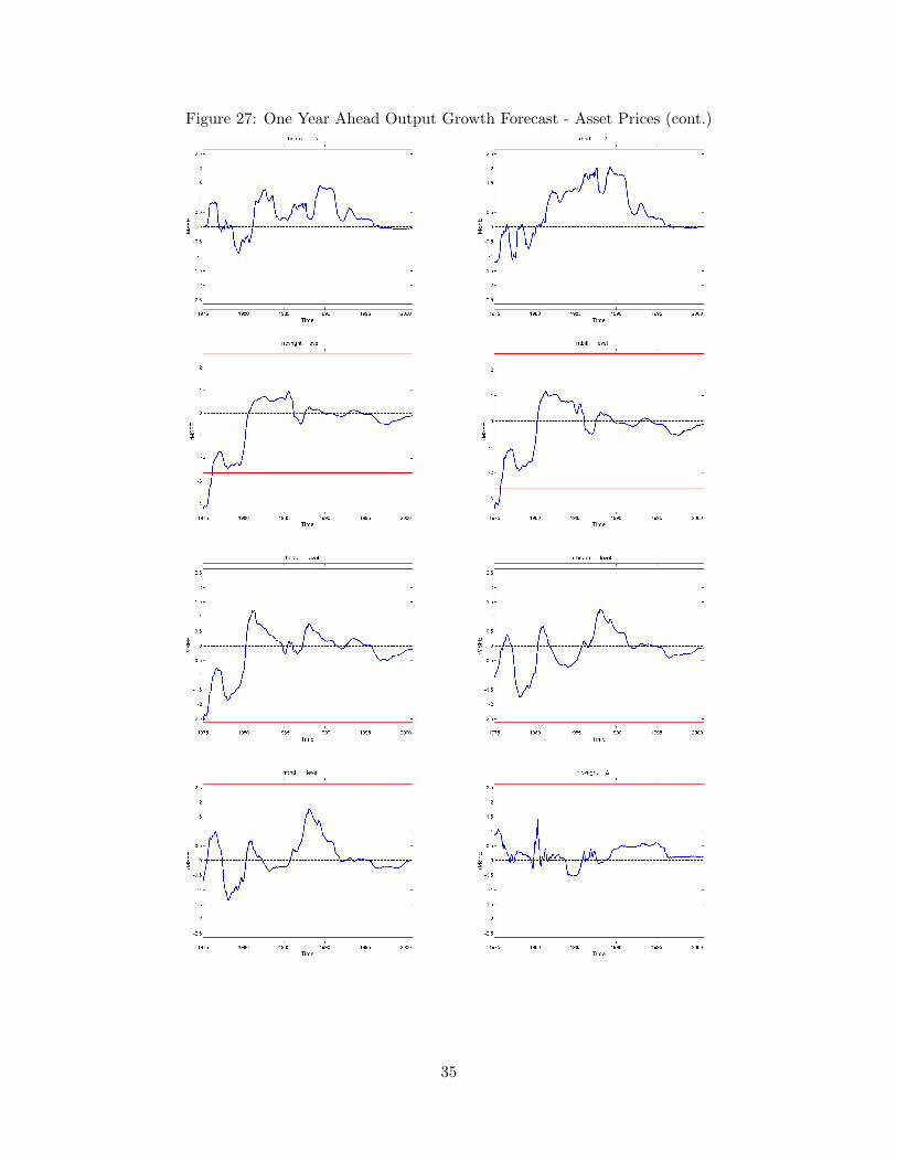
Figure 27: One Year Ahead Output Growth Forecast - Asset Prices (cont.)
35
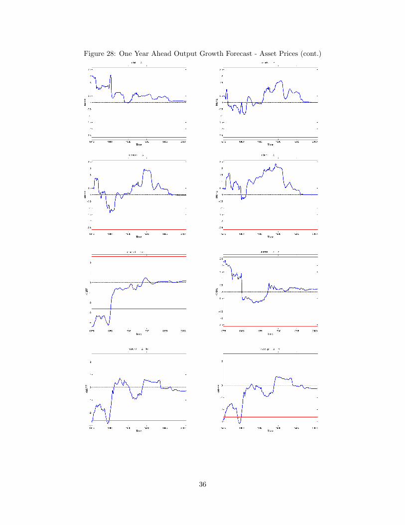
Figure 28: One Year Ahead Output Growth Forecast - Asset Prices (cont.)
36
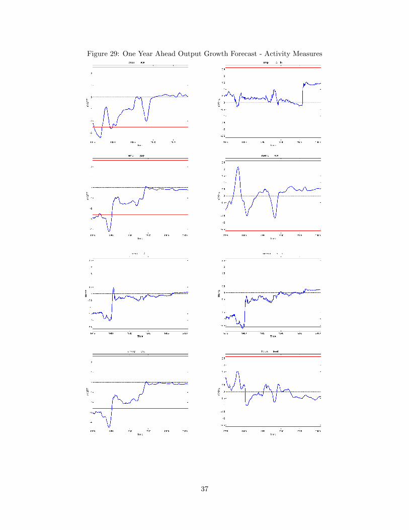
Figure 29: One Year Ahead Output Growth Forecast - Activity Measures
37
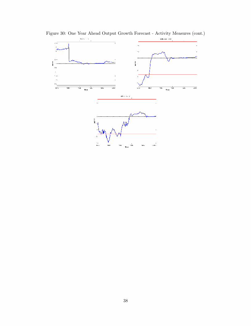
Figure 30: One Year Ahead Output Growth Forecast - Activity Measures (cont.)
38
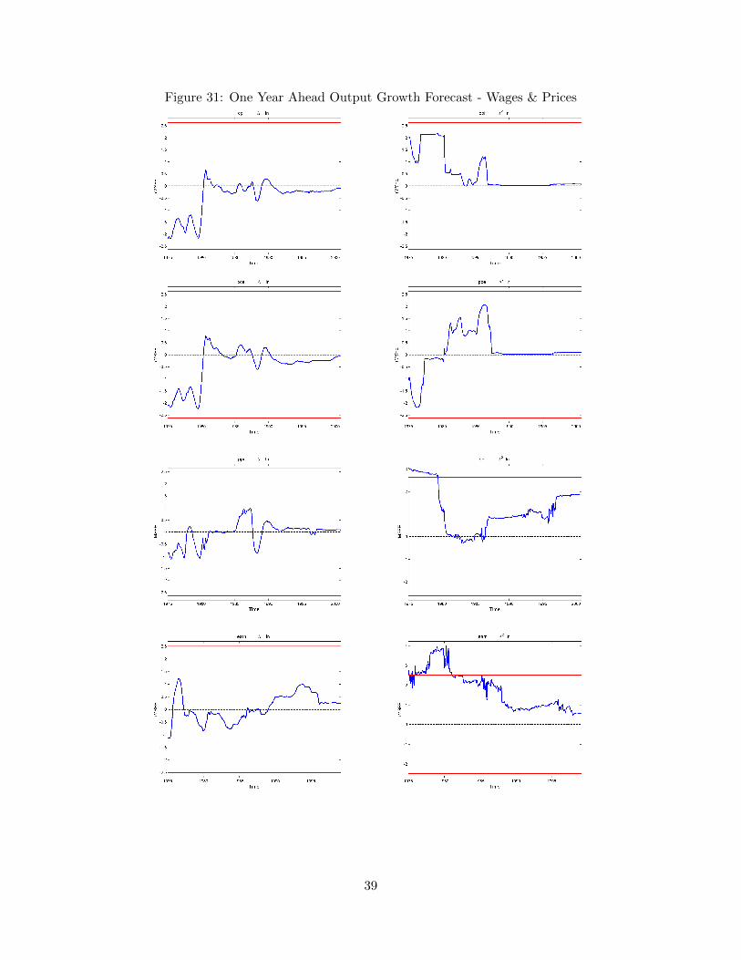
Figure 31: One Year Ahead Output Growth Forecast - Wages & Prices
39
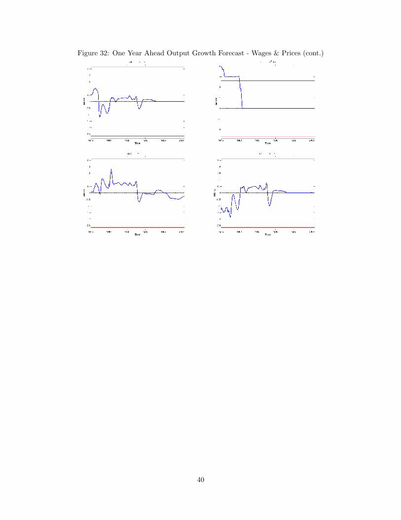
Figure 32: One Year Ahead Output Growth Forecast - Wages & Prices (cont.)
40
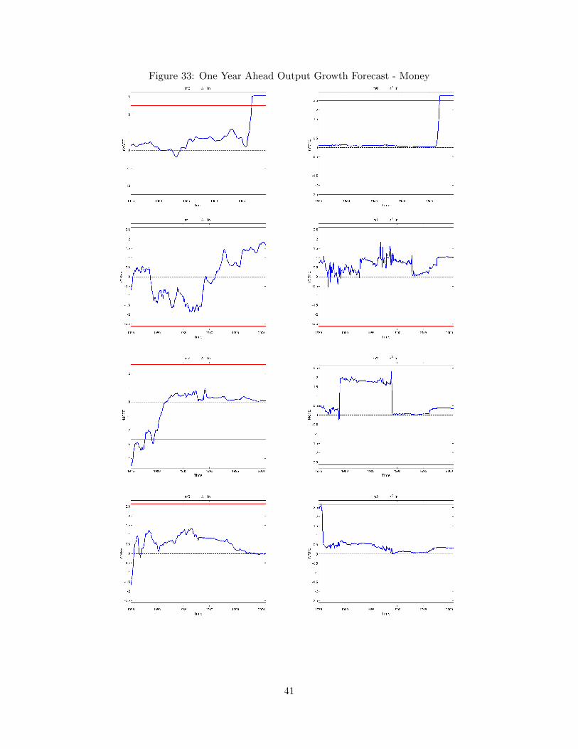
Figure 33: One Year Ahead Output Growth Forecast - Money
41
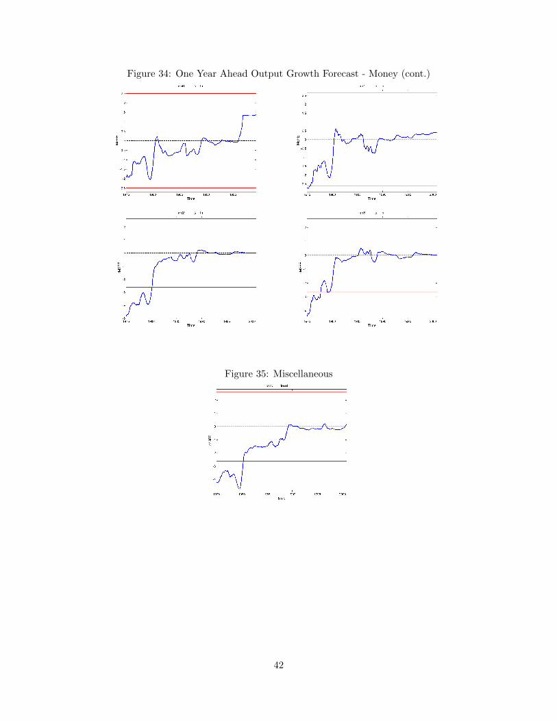
Figure 34: One Year Ahead Output Growth Forecast - Money (cont.)
Figure 35: Miscellaneous
42

Table 8: Forecasting Output Growth: Tests of Average Equal Predictive Ability
Variable rMSFE p-value Variable rMSFE p-value
rovnght level -2.17 0.03 unemp ∆ln -1.16 0.25rtbill level -1.68 0.09 unemp gap -2.87 0.00rbnds level -1.50 0.13 hours level 0.16 0.87rbndm level -0.75 0.46 hours ∆ 1.14 0.26rbndl level -0.86 0.39 deliveries level -1.65 0.10rovnght ∆ -0.23 0.82 deliveries ∆ -1.72 0.08rtbill ∆ 1.11 0.27 cpi ∆ln -1.44 0.15rbnds ∆ 0.82 0.41 cpi ∆2ln 1.21 0.23rbndm ∆ 0.28 0.78 pce ∆ln -1.30 0.19rbndl ∆ 0.20 0.84 pce ∆2ln 0.00 1.00rrovnght level -1.98 0.05 ppi ∆ln -0.29 0.77rrtbill level -1.66 0.10 ppi ∆2ln 3.06 0.00rrbnds level -1.46 0.15 earn ∆ln -0.45 0.65rrbndm level -0.78 0.43 earn ∆2ln 3.39 0.00rrbndl level -0.35 0.72 oil ∆ln 0.40 0.69rrovnght ∆ 0.59 0.56 oil ∆2ln 2.10 0.04rrtbill ∆ 1.35 0.18 roil ln 0.22 0.83rrbnds ∆ 0.64 0.52 roil ∆ln -0.39 0.70rrbndm ∆ 0.53 0.60 m0 ∆ln 2.19 0.03rrbndl ∆ 1.14 0.25 m0 ∆2ln 1.63 0.10rspread level -2.59 0.01 m1 ∆ln -0.17 0.86exrate ∆ln 1.09 0.28 m1 ∆2ln 1.40 0.16stockp ∆ln -1.56 0.12 m2 ∆ln -2.03 0.04rstockp ∆ln -1.74 0.08 m2 ∆2ln 1.39 0.16ip ∆ln - - m3 ∆ln -0.04 0.97ip gap - - m3 ∆2ln 1.79 0.07capu level -1.76 0.08 rm0 ∆ln -0.65 0.52emp ∆ln 1.19 0.24 rm1 ∆ln -1.27 0.20emp gap -2.53 0.01 rm2 ∆ln -2.86 0.00unemp level -0.25 0.80 rm3 ∆ln -2.30 0.02unemp ∆ -0.93 0.35 lead level -2.98 0.00
Note: rMSFE denotes the re-scaled average MSFE difference over the full out-of-sample period. A negative
value indicate that the model with an explanatory variable outperforms the autoregressive model); p-value
is the full out-of-sample test p-value.
43
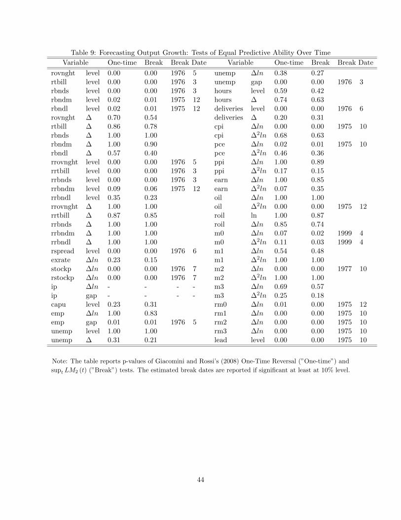
Table 9: Forecasting Output Growth: Tests of Equal Predictive Ability Over Time
Variable One-time Break Break Date Variable One-time Break Break Date
rovnght level 0.00 0.00 1976 5 unemp ∆ln 0.38 0.27rtbill level 0.00 0.00 1976 3 unemp gap 0.00 0.00 1976 3rbnds level 0.00 0.00 1976 3 hours level 0.59 0.42rbndm level 0.02 0.01 1975 12 hours ∆ 0.74 0.63rbndl level 0.02 0.01 1975 12 deliveries level 0.00 0.00 1976 6rovnght ∆ 0.70 0.54 deliveries ∆ 0.20 0.31rtbill ∆ 0.86 0.78 cpi ∆ln 0.00 0.00 1975 10rbnds ∆ 1.00 1.00 cpi ∆2ln 0.68 0.63rbndm ∆ 1.00 0.90 pce ∆ln 0.02 0.01 1975 10rbndl ∆ 0.57 0.40 pce ∆2ln 0.46 0.36rrovnght level 0.00 0.00 1976 5 ppi ∆ln 1.00 0.89rrtbill level 0.00 0.00 1976 3 ppi ∆2ln 0.17 0.15rrbnds level 0.00 0.00 1976 3 earn ∆ln 1.00 0.85rrbndm level 0.09 0.06 1975 12 earn ∆2ln 0.07 0.35rrbndl level 0.35 0.23 oil ∆ln 1.00 1.00rrovnght ∆ 1.00 1.00 oil ∆2ln 0.00 0.00 1975 12rrtbill ∆ 0.87 0.85 roil ln 1.00 0.87rrbnds ∆ 1.00 1.00 roil ∆ln 0.85 0.74rrbndm ∆ 1.00 1.00 m0 ∆ln 0.07 0.02 1999 4rrbndl ∆ 1.00 1.00 m0 ∆2ln 0.11 0.03 1999 4rspread level 0.00 0.00 1976 6 m1 ∆ln 0.54 0.48exrate ∆ln 0.23 0.15 m1 ∆2ln 1.00 1.00stockp ∆ln 0.00 0.00 1976 7 m2 ∆ln 0.00 0.00 1977 10rstockp ∆ln 0.00 0.00 1976 7 m2 ∆2ln 1.00 1.00ip ∆ln - - - - m3 ∆ln 0.69 0.57ip gap - - - - m3 ∆2ln 0.25 0.18capu level 0.23 0.31 rm0 ∆ln 0.01 0.00 1975 12emp ∆ln 1.00 0.83 rm1 ∆ln 0.00 0.00 1975 10emp gap 0.01 0.01 1976 5 rm2 ∆ln 0.00 0.00 1975 10unemp level 1.00 1.00 rm3 ∆ln 0.00 0.00 1975 10unemp ∆ 0.31 0.21 lead level 0.00 0.00 1975 10
Note: The table reports p-values of Giacomini and Rossi’s (2008) One-Time Reversal (”One-time”) and
supt LM2 (t) (”Break”) tests. The estimated break dates are reported if significant at least at 10% level.
44
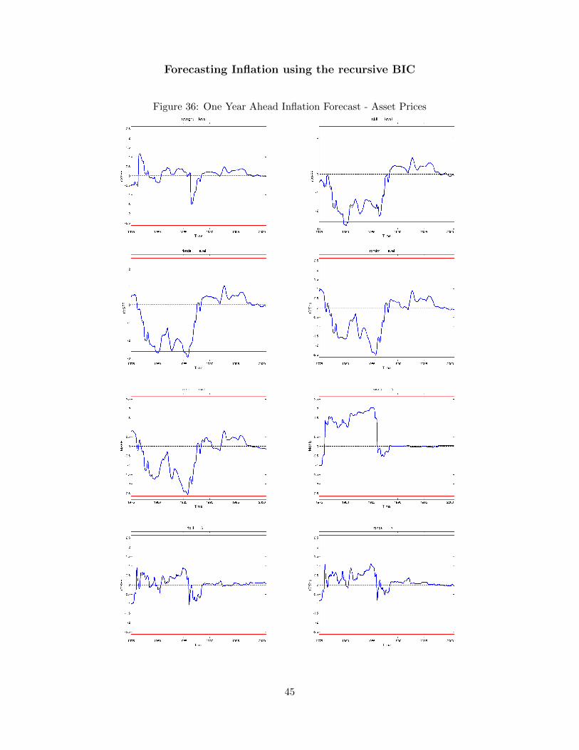
Forecasting Inflation using the recursive BIC
Figure 36: One Year Ahead Inflation Forecast - Asset Prices
45
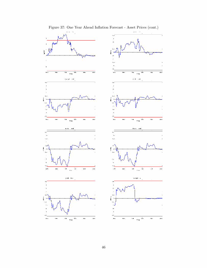
Figure 37: One Year Ahead Inflation Forecast - Asset Prices (cont.)
46
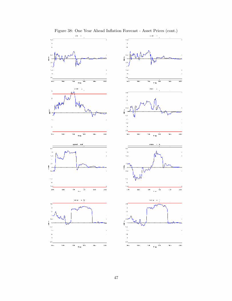
Figure 38: One Year Ahead Inflation Forecast - Asset Prices (cont.)
47
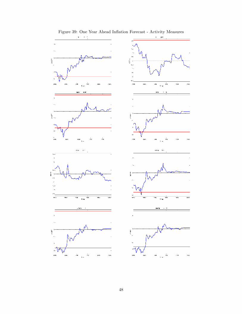
Figure 39: One Year Ahead Inflation Forecast - Activity Measures
48
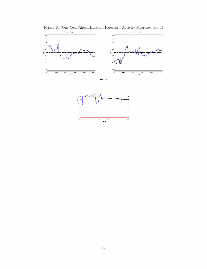
Figure 40: One Year Ahead Inflation Forecast - Activity Measures (cont.)
49
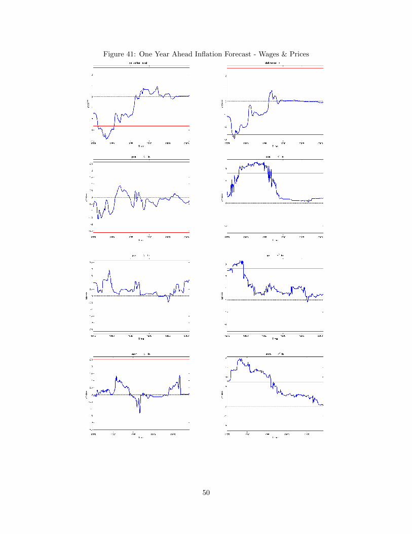
Figure 41: One Year Ahead Inflation Forecast - Wages & Prices
50
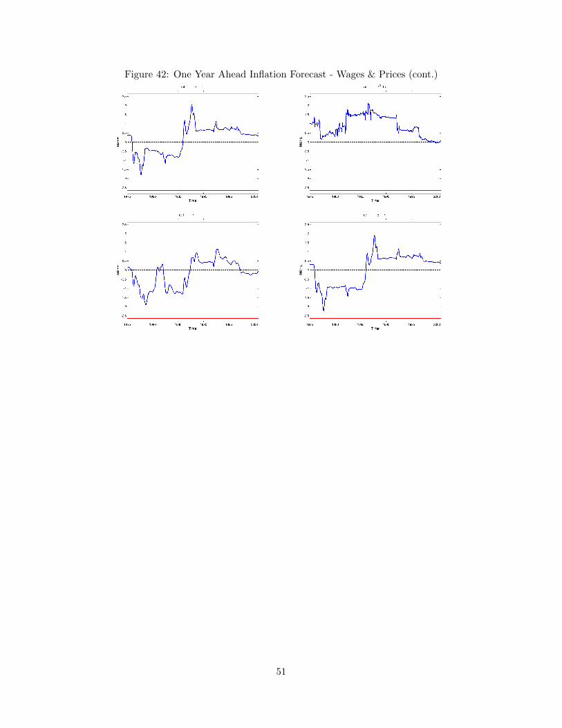
Figure 42: One Year Ahead Inflation Forecast - Wages & Prices (cont.)
51
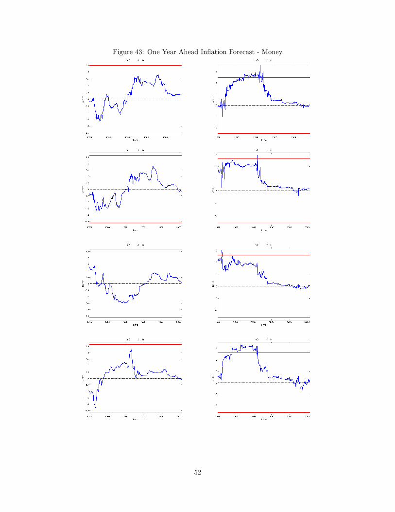
Figure 43: One Year Ahead Inflation Forecast - Money
52
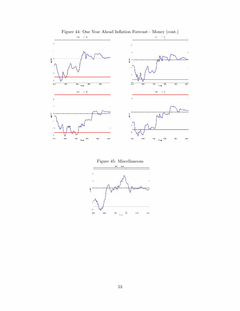
Figure 44: One Year Ahead Inflation Forecast - Money (cont.)
Figure 45: Miscellaneous
53
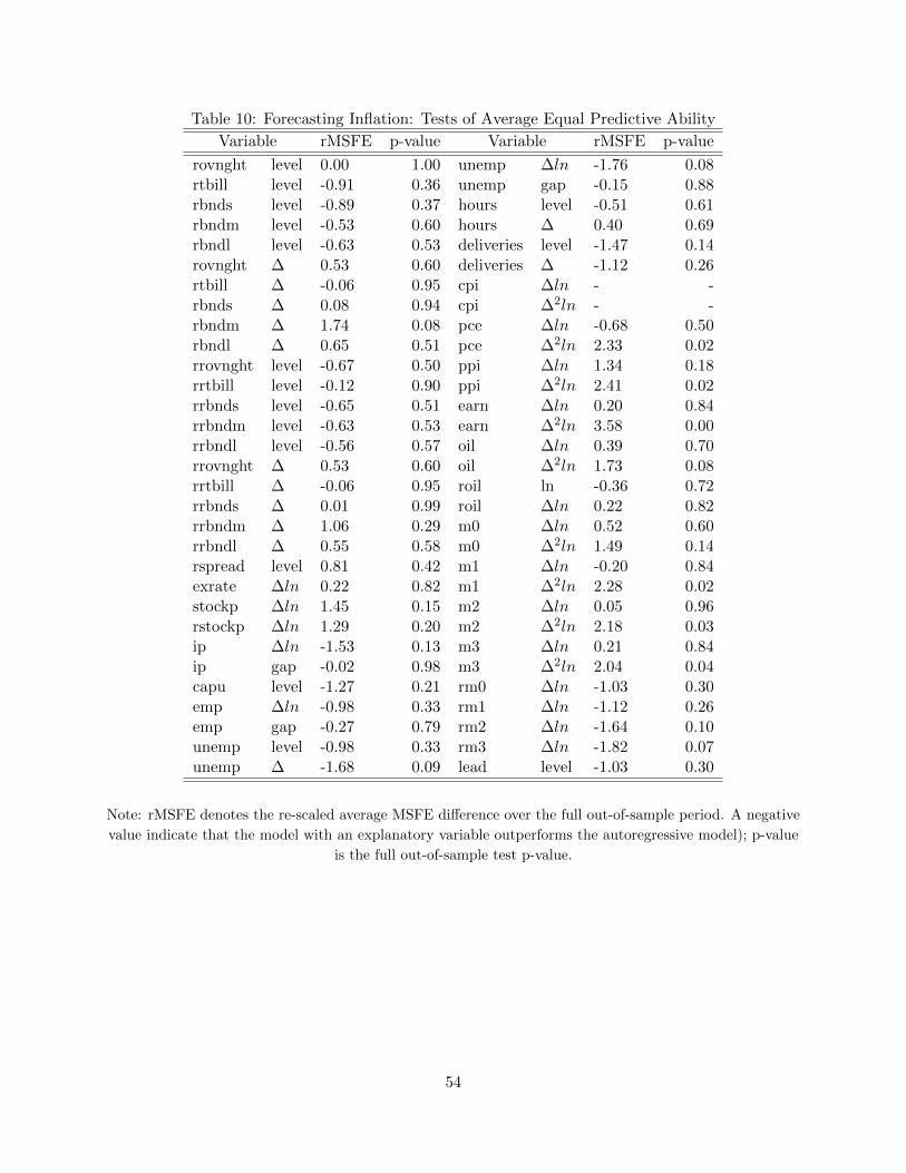
Table 10: Forecasting Inflation: Tests of Average Equal Predictive Ability
Variable rMSFE p-value Variable rMSFE p-value
rovnght level 0.00 1.00 unemp ∆ln -1.76 0.08rtbill level -0.91 0.36 unemp gap -0.15 0.88rbnds level -0.89 0.37 hours level -0.51 0.61rbndm level -0.53 0.60 hours ∆ 0.40 0.69rbndl level -0.63 0.53 deliveries level -1.47 0.14rovnght ∆ 0.53 0.60 deliveries ∆ -1.12 0.26rtbill ∆ -0.06 0.95 cpi ∆ln - -rbnds ∆ 0.08 0.94 cpi ∆2ln - -rbndm ∆ 1.74 0.08 pce ∆ln -0.68 0.50rbndl ∆ 0.65 0.51 pce ∆2ln 2.33 0.02rrovnght level -0.67 0.50 ppi ∆ln 1.34 0.18rrtbill level -0.12 0.90 ppi ∆2ln 2.41 0.02rrbnds level -0.65 0.51 earn ∆ln 0.20 0.84rrbndm level -0.63 0.53 earn ∆2ln 3.58 0.00rrbndl level -0.56 0.57 oil ∆ln 0.39 0.70rrovnght ∆ 0.53 0.60 oil ∆2ln 1.73 0.08rrtbill ∆ -0.06 0.95 roil ln -0.36 0.72rrbnds ∆ 0.01 0.99 roil ∆ln 0.22 0.82rrbndm ∆ 1.06 0.29 m0 ∆ln 0.52 0.60rrbndl ∆ 0.55 0.58 m0 ∆2ln 1.49 0.14rspread level 0.81 0.42 m1 ∆ln -0.20 0.84exrate ∆ln 0.22 0.82 m1 ∆2ln 2.28 0.02stockp ∆ln 1.45 0.15 m2 ∆ln 0.05 0.96rstockp ∆ln 1.29 0.20 m2 ∆2ln 2.18 0.03ip ∆ln -1.53 0.13 m3 ∆ln 0.21 0.84ip gap -0.02 0.98 m3 ∆2ln 2.04 0.04capu level -1.27 0.21 rm0 ∆ln -1.03 0.30emp ∆ln -0.98 0.33 rm1 ∆ln -1.12 0.26emp gap -0.27 0.79 rm2 ∆ln -1.64 0.10unemp level -0.98 0.33 rm3 ∆ln -1.82 0.07unemp ∆ -1.68 0.09 lead level -1.03 0.30
Note: rMSFE denotes the re-scaled average MSFE difference over the full out-of-sample period. A negative
value indicate that the model with an explanatory variable outperforms the autoregressive model); p-value
is the full out-of-sample test p-value.
54
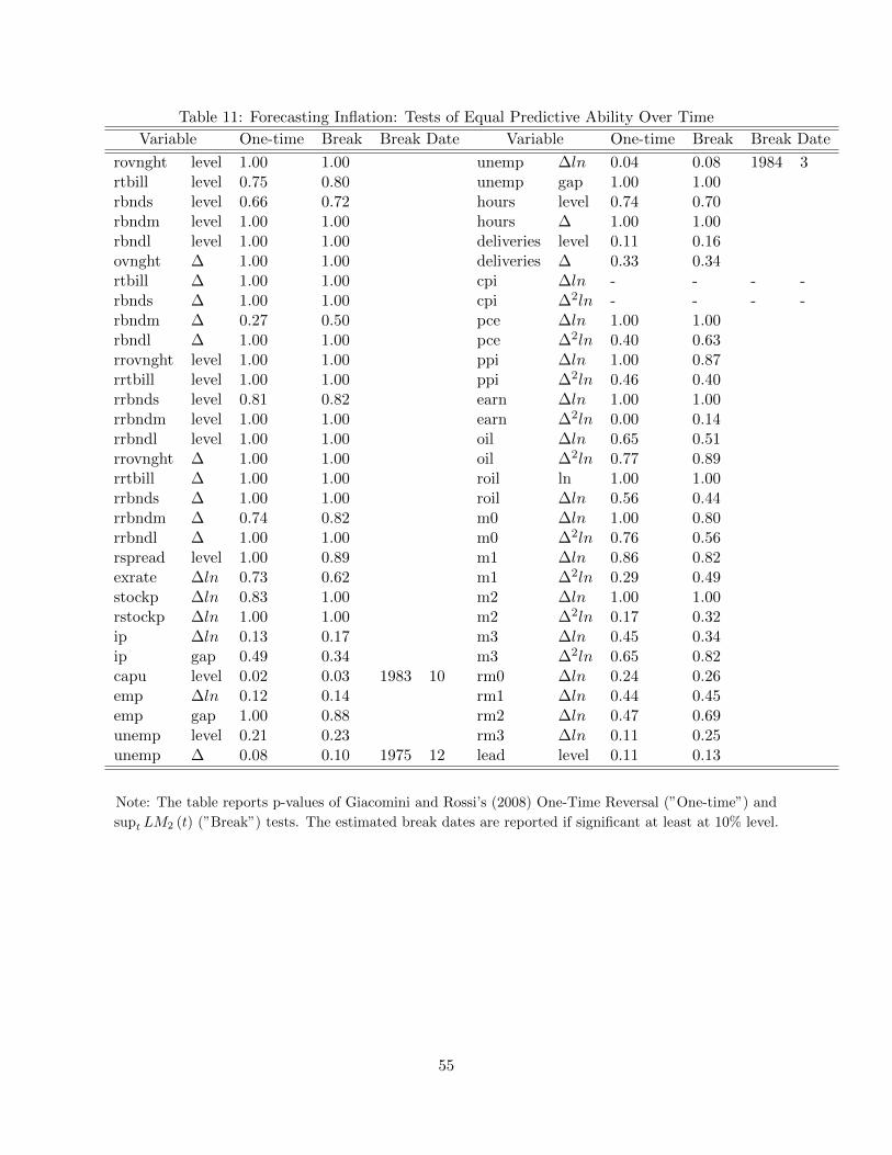
Table 11: Forecasting Inflation: Tests of Equal Predictive Ability Over Time
Variable One-time Break Break Date Variable One-time Break Break Date
rovnght level 1.00 1.00 unemp ∆ln 0.04 0.08 1984 3rtbill level 0.75 0.80 unemp gap 1.00 1.00rbnds level 0.66 0.72 hours level 0.74 0.70rbndm level 1.00 1.00 hours ∆ 1.00 1.00rbndl level 1.00 1.00 deliveries level 0.11 0.16ovnght ∆ 1.00 1.00 deliveries ∆ 0.33 0.34rtbill ∆ 1.00 1.00 cpi ∆ln - - - -rbnds ∆ 1.00 1.00 cpi ∆2ln - - - -rbndm ∆ 0.27 0.50 pce ∆ln 1.00 1.00rbndl ∆ 1.00 1.00 pce ∆2ln 0.40 0.63rrovnght level 1.00 1.00 ppi ∆ln 1.00 0.87rrtbill level 1.00 1.00 ppi ∆2ln 0.46 0.40rrbnds level 0.81 0.82 earn ∆ln 1.00 1.00rrbndm level 1.00 1.00 earn ∆2ln 0.00 0.14rrbndl level 1.00 1.00 oil ∆ln 0.65 0.51rrovnght ∆ 1.00 1.00 oil ∆2ln 0.77 0.89rrtbill ∆ 1.00 1.00 roil ln 1.00 1.00rrbnds ∆ 1.00 1.00 roil ∆ln 0.56 0.44rrbndm ∆ 0.74 0.82 m0 ∆ln 1.00 0.80rrbndl ∆ 1.00 1.00 m0 ∆2ln 0.76 0.56rspread level 1.00 0.89 m1 ∆ln 0.86 0.82exrate ∆ln 0.73 0.62 m1 ∆2ln 0.29 0.49stockp ∆ln 0.83 1.00 m2 ∆ln 1.00 1.00rstockp ∆ln 1.00 1.00 m2 ∆2ln 0.17 0.32ip ∆ln 0.13 0.17 m3 ∆ln 0.45 0.34ip gap 0.49 0.34 m3 ∆2ln 0.65 0.82capu level 0.02 0.03 1983 10 rm0 ∆ln 0.24 0.26emp ∆ln 0.12 0.14 rm1 ∆ln 0.44 0.45emp gap 1.00 0.88 rm2 ∆ln 0.47 0.69unemp level 0.21 0.23 rm3 ∆ln 0.11 0.25unemp ∆ 0.08 0.10 1975 12 lead level 0.11 0.13
Note: The table reports p-values of Giacomini and Rossi’s (2008) One-Time Reversal (”One-time”) and
supt LM2 (t) (”Break”) tests. The estimated break dates are reported if significant at least at 10% level.
55

Section 3: Robustness to the choice of window size
56
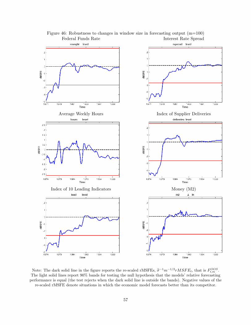
Figure 46: Robustness to changes in window size in forecasting output (m=100)Federal Funds Rate Interest Rate Spread
Average Weekly Hours Index of Supplier Deliveries
Index of 10 Leading Indicators Money (M2)
Note: The dark solid line in the figure reports the re-scaled rMSFEs, σ̂−1m−1/2rMSFEt, that is FOOSt,m .
The light solid lines report 90% bands for testing the null hypothesis that the models’ relative forecastingperformance is equal (the test rejects when the dark solid line is outside the bands). Negative values of the
re-scaled rMSFE denote situations in which the economic model forecasts better than its competitor.
57
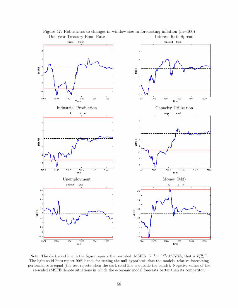
Figure 47: Robustness to changes in window size in forecasting inflation (m=100)One-year Treasury Bond Rate Interest Rate Spread
Industrial Production Capacity Utilization
Unemployment Money (M3)
Note: The dark solid line in the figure reports the re-scaled rMSFEs, σ̂−1m−1/2rMSFEt, that is FOOSt,m .
The light solid lines report 90% bands for testing the null hypothesis that the models’ relative forecastingperformance is equal (the test rejects when the dark solid line is outside the bands). Negative values of the
re-scaled rMSFE denote situations in which the economic model forecasts better than its competitor.
58
Section 4: Robustness to Consumption Deflator-based measuresof Inflation
59
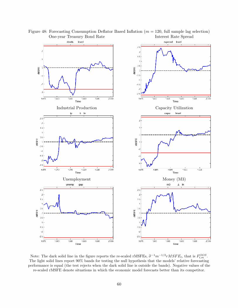
Figure 48: Forecasting Consumption Deflator Based Inflation (m = 120, full sample lag selection)One-year Treasury Bond Rate Interest Rate Spread
Industrial Production Capacity Utilization
Unemployment Money (M3)
Note: The dark solid line in the figure reports the re-scaled rMSFEs, σ̂−1m−1/2rMSFEt, that is FOOSt,m .
The light solid lines report 90% bands for testing the null hypothesis that the models’ relative forecastingperformance is equal (the test rejects when the dark solid line is outside the bands). Negative values of the
re-scaled rMSFE denote situations in which the economic model forecasts better than its competitor.
60
Section 5: Robustness to changes in variance
61
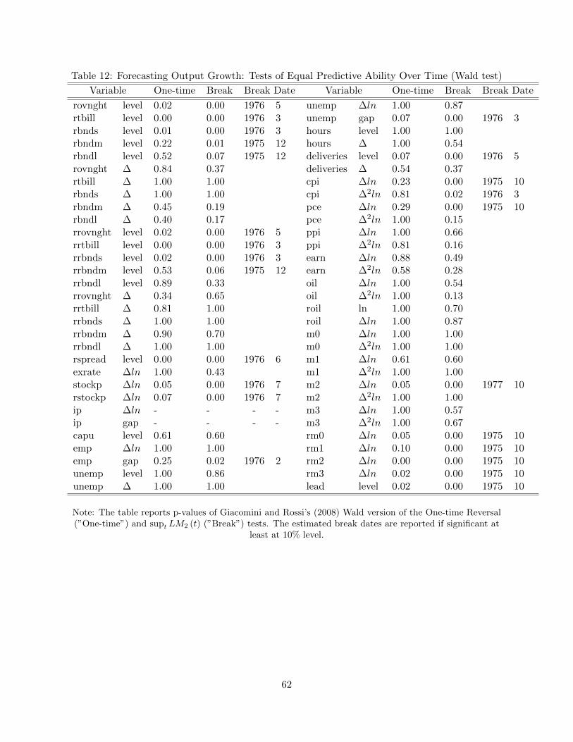
Table 12: Forecasting Output Growth: Tests of Equal Predictive Ability Over Time (Wald test)
Variable One-time Break Break Date Variable One-time Break Break Date
rovnght level 0.02 0.00 1976 5 unemp ∆ln 1.00 0.87rtbill level 0.00 0.00 1976 3 unemp gap 0.07 0.00 1976 3rbnds level 0.01 0.00 1976 3 hours level 1.00 1.00rbndm level 0.22 0.01 1975 12 hours ∆ 1.00 0.54rbndl level 0.52 0.07 1975 12 deliveries level 0.07 0.00 1976 5rovnght ∆ 0.84 0.37 deliveries ∆ 0.54 0.37rtbill ∆ 1.00 1.00 cpi ∆ln 0.23 0.00 1975 10rbnds ∆ 1.00 1.00 cpi ∆2ln 0.81 0.02 1976 3rbndm ∆ 0.45 0.19 pce ∆ln 0.29 0.00 1975 10rbndl ∆ 0.40 0.17 pce ∆2ln 1.00 0.15rrovnght level 0.02 0.00 1976 5 ppi ∆ln 1.00 0.66rrtbill level 0.00 0.00 1976 3 ppi ∆2ln 0.81 0.16rrbnds level 0.02 0.00 1976 3 earn ∆ln 0.88 0.49rrbndm level 0.53 0.06 1975 12 earn ∆2ln 0.58 0.28rrbndl level 0.89 0.33 oil ∆ln 1.00 0.54rrovnght ∆ 0.34 0.65 oil ∆2ln 1.00 0.13rrtbill ∆ 0.81 1.00 roil ln 1.00 0.70rrbnds ∆ 1.00 1.00 roil ∆ln 1.00 0.87rrbndm ∆ 0.90 0.70 m0 ∆ln 1.00 1.00rrbndl ∆ 1.00 1.00 m0 ∆2ln 1.00 1.00rspread level 0.00 0.00 1976 6 m1 ∆ln 0.61 0.60exrate ∆ln 1.00 0.43 m1 ∆2ln 1.00 1.00stockp ∆ln 0.05 0.00 1976 7 m2 ∆ln 0.05 0.00 1977 10rstockp ∆ln 0.07 0.00 1976 7 m2 ∆2ln 1.00 1.00ip ∆ln - - - - m3 ∆ln 1.00 0.57ip gap - - - - m3 ∆2ln 1.00 0.67capu level 0.61 0.60 rm0 ∆ln 0.05 0.00 1975 10emp ∆ln 1.00 1.00 rm1 ∆ln 0.10 0.00 1975 10emp gap 0.25 0.02 1976 2 rm2 ∆ln 0.00 0.00 1975 10unemp level 1.00 0.86 rm3 ∆ln 0.02 0.00 1975 10unemp ∆ 1.00 1.00 lead level 0.02 0.00 1975 10
Note: The table reports p-values of Giacomini and Rossi’s (2008) Wald version of the One-time Reversal(”One-time”) and supt LM2 (t) (”Break”) tests. The estimated break dates are reported if significant at
least at 10% level.
62
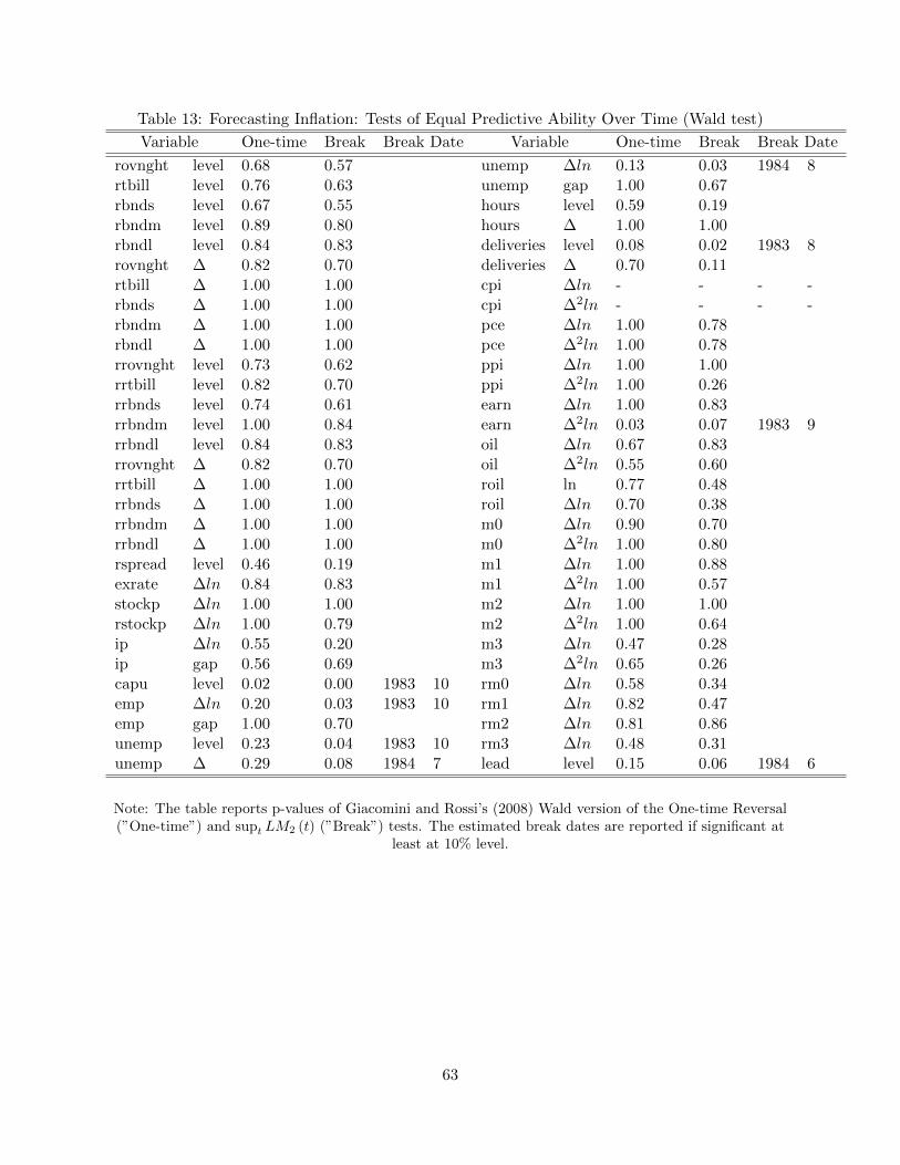
Table 13: Forecasting Inflation: Tests of Equal Predictive Ability Over Time (Wald test)
Variable One-time Break Break Date Variable One-time Break Break Date
rovnght level 0.68 0.57 unemp ∆ln 0.13 0.03 1984 8rtbill level 0.76 0.63 unemp gap 1.00 0.67rbnds level 0.67 0.55 hours level 0.59 0.19rbndm level 0.89 0.80 hours ∆ 1.00 1.00rbndl level 0.84 0.83 deliveries level 0.08 0.02 1983 8rovnght ∆ 0.82 0.70 deliveries ∆ 0.70 0.11rtbill ∆ 1.00 1.00 cpi ∆ln - - - -rbnds ∆ 1.00 1.00 cpi ∆2ln - - - -rbndm ∆ 1.00 1.00 pce ∆ln 1.00 0.78rbndl ∆ 1.00 1.00 pce ∆2ln 1.00 0.78rrovnght level 0.73 0.62 ppi ∆ln 1.00 1.00rrtbill level 0.82 0.70 ppi ∆2ln 1.00 0.26rrbnds level 0.74 0.61 earn ∆ln 1.00 0.83rrbndm level 1.00 0.84 earn ∆2ln 0.03 0.07 1983 9rrbndl level 0.84 0.83 oil ∆ln 0.67 0.83rrovnght ∆ 0.82 0.70 oil ∆2ln 0.55 0.60rrtbill ∆ 1.00 1.00 roil ln 0.77 0.48rrbnds ∆ 1.00 1.00 roil ∆ln 0.70 0.38rrbndm ∆ 1.00 1.00 m0 ∆ln 0.90 0.70rrbndl ∆ 1.00 1.00 m0 ∆2ln 1.00 0.80rspread level 0.46 0.19 m1 ∆ln 1.00 0.88exrate ∆ln 0.84 0.83 m1 ∆2ln 1.00 0.57stockp ∆ln 1.00 1.00 m2 ∆ln 1.00 1.00rstockp ∆ln 1.00 0.79 m2 ∆2ln 1.00 0.64ip ∆ln 0.55 0.20 m3 ∆ln 0.47 0.28ip gap 0.56 0.69 m3 ∆2ln 0.65 0.26capu level 0.02 0.00 1983 10 rm0 ∆ln 0.58 0.34emp ∆ln 0.20 0.03 1983 10 rm1 ∆ln 0.82 0.47emp gap 1.00 0.70 rm2 ∆ln 0.81 0.86unemp level 0.23 0.04 1983 10 rm3 ∆ln 0.48 0.31unemp ∆ 0.29 0.08 1984 7 lead level 0.15 0.06 1984 6
Note: The table reports p-values of Giacomini and Rossi’s (2008) Wald version of the One-time Reversal(”One-time”) and supt LM2 (t) (”Break”) tests. The estimated break dates are reported if significant at
least at 10% level.
63