École de technologie supÉrieure …espace.etsmtl.ca/1843/1/ben_mosbah_abdallah_thèse.pdf · i...

ÉCOLE DE TECHNOLOGIE SUPÉRIEURE UNIVERSITÉ DU QUÉBEC

MANUSCRIPT-BASED THESIS PRESENTED TO ÉCOLE DE TECHNOLOGIE SUPÉRIEURE

IN PARTIAL FULFILLMENT OF THE REQUIREMENTS FOR THE DEGREE OF DOCTOR OF PHILOSOPHY

Ph.D.

BY Abdallah BEN MOSBAH

NEW METHODOLOGIES FOR CALCULATION OF FLIGHT PARAMETERS ON REDUCED SCALE WINGS MODELS IN WIND TUNNEL

MONTREAL, JANUARY 4TH, 2017

© Copyright 2016 reserved by Abdallah Ben Mosbah

© Copyright reserved

It is forbidden to reproduce, save or share the content of this document either in whole or in parts. The reader

who wishes to print or save this document on any media must first get the permission of the author.

BOARD OF EXAMINERS (THESIS PH.D.)

THIS THESIS HAS BEEN EVALUATED

BY THE FOLLOWING BOARD OF EXAMINERS Dr. Ruxandra Mihaela Botez, Thesis Supervisor Department of Automated Production Engineering at École de technologie supérieure Dr. Thien-My Dao, Thesis Co-supervisor Department of Mechanical Engineering at École de technologie supérieure Dr. Ammar Kouki, President of the Board of Examiners Department of Electrical Engineering at École de technologie supérieure Dr. Pascal Bigras, Member of the jury Department of Automated Production Engineering at École de technologie supérieure Dr. Nabil Nahas, External Evaluator Department of System Engineering at King Fahd University of Petroleum and Minerals

THIS THESIS WAS PRENSENTED AND DEFENDED

IN THE PRESENCE OF A BOARD OF EXAMINERS AND PUBLIC

MONTREAL, NOVEMBER 25TH, 2016

AT ÉCOLE DE TECHNOLOGIE SUPÉRIEURE

ACKNOWLEDGMENT

First, I thank God for his favors and gratitude to provide me the patience and knowledge to

complete my dissertation.

It gives me particular pleasure, before presenting my work to express my gratitude to those

near and far have given me their concern. I especially express my deep appreciation to my

research supervisors, Ruxandra Botez and Thien-My Dao for their guidance and kindness

throughout this work.

A special thanks to Mr. Nabil Nahas, Mr. Pascal Bigras and Mr Ammar Kouki for taking

time to evaluate this work and to serve on my thesis committee.

I am very thankful to all my colleagues of LARCASE team for their helpful discussions.

I express a big thankful to my dear wife Soumaya and my siblings who supported,

encouraged and helped me to cap off my thesis. I also thank all my friends for their

confidence and support.

An enormous thanks to my parents, Salem and Om Essaed, for the support and love given to

me to achieve my dream. I cannot thank them enough for all the sacrifices they made during

every phase of this thesis. No reward or dedication cannot express my gratitude and deep

respect and love.

Finally, I would like to dedicate this work to all my family especially to my children Iyess

and Anas in spite of spending so much time away from them to achieve this work.

NOUVELLES MÉTHODOLOGIES DE CALCUL DES PARAMÈTRES DE VOL SUR DES MODÈLES DES AILES À L'ÉCHELLE RÉDUITE EN SOUFFLERIE

Abdallah BEN MOSBAH

RÉSUMÉ

Dans le but d'améliorer les qualités de tests en soufflerie ainsi que les outils nécessaires pour réaliser des tests aérodynamiques sur des modèles d'ailes d'avions en soufflerie, des nouvelles méthodologies ont été développées et testées sur des modèles d'ailes originales et déformables. Un concept d'aile déformable consiste à remplacer une partie (inférieure et/ou supérieure) de la peau de l'aile par une autre partie flexible dont sa forme peut être modifiée à l'aide d'un système d'actionnement installé à l'intérieur de l'aile. Le but d'utiliser ce concept est d'améliorer les performances aérodynamiques de l'avion et surtout de réduire sa consommation de carburant. Des analyses numériques et expérimentales ont été effectuées afin de développer et de tester les méthodologies proposées dans cette thèse. Dans l'objectif de contrôler l'étalonnage de la soufflerie Price-Païdoussis de LARCASE, des analyses numériques et expérimentales ont été réalisées. Des calculs par éléments finis ont été faits pour construire une base de données permettant de développer une nouvelle méthodologie hybride d'étalonnage. Cette nouvelle approche a permis de contrôler l'écoulement d'air dans la chambre d'essais de la soufflerie Price-Païdoussis. Pour la détermination rapide des paramètres aérodynamiques, des nouvelles méthodologies hybrides ont été proposées. Ces méthodologies ont été utilisées pour le contrôle des paramètres de vol par la détermination des coefficients de traînée et de portance, de moment de tangage ainsi que de la distribution de pression autour d'un profil d'aile d'avion. Ces coefficients aérodynamiques ont été calculés à partir des conditions d'écoulement connues comme l'angle d'attaque, le nombre de Mach et le nombre de Reynolds. Dans le but de changer la forme de la peau de l’aile, des actionneurs électriques ont été installés à l'intérieur de l'aile pour modifier sa surface supérieure et pour avoir la forme désirée. Cette déformation permet d'obtenir les profiles optimales en fonction de différentes conditions de vol afin de réduire la consommation de carburant de l'avion. Un contrôleur basé sur des réseaux de neurones a été mis en œuvre afin d'obtenir les déplacements souhaités des actionneurs. Un algorithme d'optimisation métaheuristique a été utilisée en hybridation avec des réseaux de neurones ainsi qu'avec une approche machine à vecteurs de support. Leur combinaison a été optimisée et de très bons résultats ont été obtenus dans un temps de calcul réduit. La validation des résultats obtenus par la combinaison de ces techniques a été réalisée à l'aide des données numériques du code XFoil et aussi avec le logiciel de simulation numérique

VIII

Fluent. Les résultats obtenus à l'aide des méthodologies présentées dans cette thèse ont été aussi validés par des essais expérimentaux dans la soufflerie subsonique Price-Païdoussis. Mots clés: analyse aérodynamique, optimisation, intelligence artificielle, aile déformable, validation expérimentale

NEW METHODOLOGIES FOR CALCULATION OF FLIGHT PARAMETERS ON REDUCED SCALE WINGS MODELS IN WIND TUNNEL

Abdallah BEN MOSBAH

ABSTRACT

In order to improve the qualities of wind tunnel tests, and the tools used to perform aerodynamic tests on aircraft wings in the wind tunnel, new methodologies were developed and tested on rigid and flexible wings models. A flexible wing concept is consists in replacing a portion (lower and/or upper) of the skin with another flexible portion whose shape can be changed using an actuation system installed inside of the wing. The main purpose of this concept is to improve the aerodynamic performance of the aircraft, and especially to reduce the fuel consumption of the airplane. Numerical and experimental analyses were conducted to develop and test the methodologies proposed in this thesis. To control the flow inside the test sections of the Price-Païdoussis wind tunnel of LARCASE, numerical and experimental analyses were performed. Computational fluid dynamics calculations have been made in order to obtain a database used to develop a new hybrid methodology for wind tunnel calibration. This approach allows controlling the flow in the test section of the Price-Païdoussis wind tunnel. For the fast determination of aerodynamic parameters, new hybrid methodologies were proposed. These methodologies were used to control flight parameters by the calculation of the drag, lift and pitching moment coefficients and by the calculation of the pressure distribution around an airfoil. These aerodynamic coefficients were calculated from the known airflow conditions such as angles of attack, the mach and the Reynolds numbers. In order to modify the shape of the wing skin, electric actuators were installed inside the wing to get the desired shape. These deformations provide optimal profiles according to different flight conditions in order to reduce the fuel consumption. A controller based on neural networks was implemented to obtain desired displacement actuators. A metaheuristic algorithm was used in hybridization with neural networks, and support vector machine approaches and their combination was optimized, and very good results were obtained in a reduced computing time. The validation of the obtained results has been made using numerical data obtained by the XFoil code, and also by the Fluent code. The results obtained using the methodologies presented in this thesis have been validated with experimental data obtained using the subsonic Price-Païdoussis blow down wind tunnel. Keywords: aerodynamic analyses, optimization, artificial intelligence, morphing wing,

experimental validation

TABLE OF CONTENTS

INTRODUCTION .....................................................................................................................1

CHAPTER 1 LITTERATURE REVIEW ................................................................................13 1.1 Hybrid Approaches ......................................................................................................13

1.1.1 Neural Networks and Fuzzy Logic ........................................................... 13 1.1.2 Artificial intelligence and optimization algorithms .................................. 14

1.1.2.1 The Simulated Annealing .......................................................... 15 1.1.2.2 The Genetic Algorithm .............................................................. 16

1.2 Neural Networks in Wind Tunnel Applications ..........................................................17 1.3 Support Vector Machines ............................................................................................20

CHAPTER 2 APPROACH AND THESIS ORGANIZATION ..............................................23 2.1 Thesis Research Approach ...........................................................................................23 2.2 Thesis Organization .....................................................................................................24

2.2.1 First journal paper ..................................................................................... 25 2.2.2 Second journal paper ................................................................................. 25 2.2.3 Third journal paper ................................................................................... 26 2.2.4 Fourth journal paper .................................................................................. 26

CHAPTER 3 ARTICLE 1: NEW METHODOLOGY FOR WIND TUNNEL CALIBRATION USING NEURAL NETWORKS - EGD APPROACH ..........29

3.1 Introduction ..................................................................................................................31 3.2 Subsonic wind tunnel ...................................................................................................32 3.3 Flow characterisation ...................................................................................................35

3.3.1 The Log-Tchebycheff Method .................................................................. 36 3.4 Extended great deluge technique .................................................................................38 3.5 Neural network approach .............................................................................................41

3.5.1 Implementation of neural networks and Preliminary results: ................... 43 3.6 Conclusion ...................................................................................................................45

CHAPTER 4 ARTICLE 2: A HYBRID ORIGINAL APPROACH FOR PREDICTION OF THE AERODYNAMIC COEFFICIENTS OF AN ATR-42 SCALED WING MODEL ..............................................................................................................47

4.1 Introduction ..................................................................................................................48 4.2 Support vector machines (SVM) .................................................................................51 4.3 Optimization of the SVM parameters ..........................................................................53 4.4 Extended great deluge algorithm .................................................................................54 4.5 New proposed SVM-EGD algorithm ...........................................................................57 4.6 Infrastructure ................................................................................................................58

4.6.1 Price-Païdoussis wind tunnel .................................................................... 58 4.6.2 Transducer ................................................................................................. 60 4.6.3 ATR-42 wing ............................................................................................ 61

4.7 Implementation of the SVM-EGD algorithm and analysis of results ..........................62 4.7.1 Theoretical results ..................................................................................... 62

XII

4.7.2 Experimental results.................................................................................. 66 4.8 Conclusions ..................................................................................................................74

CHAPTER 5 ARTICLE 3: NEW METHODOLOGY COMBINING NEURAL NETWORK AND EXTENDED GREAT DELUGE ALGORITHMS FOR THE ATR-42 WING AERODYNAMICS ANALYSIS ...........................................................75

5.1 Introduction and background .......................................................................................76 5.2 Flight parameters .........................................................................................................81 5.3 XFOIL code .................................................................................................................82 5.4 Neural networks ...........................................................................................................82 5.5 EXTENDED GREAT DELUGE .................................................................................84 5.6 NN-EGD ALGORITHM .............................................................................................86 5.7 Implementation of NN-EGD and theoretical results ...................................................87

5.7.1 The CL, CD and CM prediction system ....................................................... 89 5.7.2 The Cp prediction system ......................................................................... 94

5.8 Experimental tests ........................................................................................................97 5.8.1 Equipment ................................................................................................. 97

5.9 Experimental results...................................................................................................100 5.10 Conclusion .................................................................................................................107

CHAPTER 6 ARTICLE 4: A NEURAL NETWORK CONTROLLER FOR ATR-42 MORPHING WING ACTUATION ...............................................................109

6.1 Introduction ................................................................................................................110 6.2 ATR-42 Morphing Wing Model ................................................................................112 6.3 The closed loop architecture of the model .................................................................114

6.3.1 Controller architecture ............................................................................ 114 6.3.2 Modeling of the DC motor ...................................................................... 115

6.4 Neural Network Control System Design ...................................................................118 6.5 Experimental work .....................................................................................................124

6.5.1 Concept of the experimental work .......................................................... 124 6.5.2 Experimentation and real time validation ............................................... 125

6.5.2.1 Hardware .................................................................................. 125 6.5.2.2 Real-Time Model ..................................................................... 126 6.5.2.3 Validation Results .................................................................... 127

6.5.3 Wind tunnel test ...................................................................................... 128 6.5.3.1 Experimental test equipment.................................................... 128 6.5.3.2 Experimental results................................................................. 130

6.6 Conclusion .................................................................................................................132

DISCUSSION OF RESULTS................................................................................................133

CONCLUSION AND RECOMMENDATIONS ..................................................................139

LIST OF REFERENCES .......................................................................................................143

LIST OF TABLES

Page

Table 0.1 Geometry of the ATR 42 wing models................................................................3

Table 4.1 Original versus predicted lift coefficients for different airflow cases. .............. 63

Table 4.2 Original versus predicted drag coefficients for different airflow cases. ............ 64

Table 4.3 Original versus predicted moment coefficients for different airflow cases. ...... 65

Table 4.4 Experimental versus predicted lift coefficients for different airflow cases. ...... 68

Table 4.5 Experimental versus predicted drag coefficients for different airflow cases. ... 70

Table 4.6 Experimental versus predicted moment coefficients for different airflow cases....................................................................................................................72

Table 4.7 The obtained mean squared errors. .................................................................... 73

Table 5.1 Neural network architecture for CL, CD and CM prediction ............................... 89

Table 5.2 Lift coefficients variation with the angle of attack ............................................ 92

Table 5.3 Drag coefficients variation with the angle of attack .......................................... 92

Table 5.4 Moment coefficients variation with the angle of attack .................................... 93

Table 5.5 Neural network architecture for Cp prediction .................................................. 95

Table 5.6 Location of pressure taps along the chord ....................................................... 100

Table 5.7 Cp values residual error between the NN-EGD, XFoil and experimental results for α=2.3o ............................................................................................................................................... 101

Table 5.8 Cp values residual error between the NN-EGD, XFoil and experimental results for α=-2o ............................................................................................... 101

Table 5.9 Test parameters ................................................................................................ 103

Table 5.10 The residual error between the NN-EGD method and the experimental results................................................................................................................103

Table 6.1 Internal Motor Characteristics ......................................................................... 118

Table 6.2 ''Position controller'' database .......................................................................... 121

XIV

Table 6.3 ''Current controller'' database ........................................................................... 121

Table 6.4 List of the hardware used in the experiment .................................................... 125

Table 6.5 Location of pressure taps ................................................................................. 130

LIST OF FIGURES

Page

Figure 0.1 Reduced scale of the original wing model of an ATR 42 aircraft........................2

Figure 0.2 Original and optimized ATR 42 profile...............................................................3

Figure 0.3 General Architecture of an Artificial Neuron.......................................................6

Figure 0.4 General Principle of the SVM..............................................................................7

Figure 0.5 *,i iζ ζ variation in non-linear regression..............................................................8

Figure 0.6 Price-Païdoussis Subsonic Blow Down Wind Tunnel.......................................12

Figure 3.1 Wind tunnel sections ......................................................................................... 33

Figure 3.2 Wind tunnel measurement ................................................................................. 33

Figure 3.3 Double impeller centrifugal fan ......................................................................... 34

Figure 3.4 Settling sections ................................................................................................. 35

Figure 3.5 60 points traverse plane ..................................................................................... 37

Figure 3.6 Test section calibration ...................................................................................... 37

Figure 3.7 Pitot tube device ................................................................................................ 38

Figure 3.8 General flowchart of the EDG Taken from Ben Mosbah and Dao (2011) ......................................................... 40

Figure 3.9 Neural approach chart ........................................................................................ 42

Figure 3.10 Configuration of used NN taken from Matlab ................................................... 43

Figure 3.11 Full mesh of ATR42 profile .............................................................................. 44

Figure 3.12 Comparison of pressure theoretic and pressure predict for plane 1................... 44

Figure 3.13 Comparison of pressure theoretic and pressure predict for plane 2................... 45

Figure 3.14 Comparison of pressure theoretic and pressure predict for plane 10................. 45

Figure 4.1 Extended great deluge algorithm Take from Ben Mosbah and Dao (2011) ........................................................... 56

Figure 4.2 Price-Païdoussis wind tunnel ............................................................................. 58

XVI

Figure 4.3 Hybrid SVM-EGD algorithm Taken from Ben Mosbah et al. (2014) ............................................................... 59

Figure 4.4 Transducer ......................................................................................................... 60

Figure 4.5 Fastening system of the model and transducer .................................................. 61

Figure 4.6 ATR-42 model installed in the test chamber of the wind tunnel ....................... 62

Figure 4.7 Lift coefficient CL versus angle of attack .......................................................... 64

Figure 4.8 Drag coefficient CD versus angle of attack ........................................................ 65

Figure 4.9 Moment coefficient CM versus angle of attack .................................................. 66

Figure 4.10 Lift aerodynamic coefficients variation versus angle of attack ......................... 69

Figure 4.11 Drag aerodynamic coefficients variation versus angle of attack ....................... 71

Figure 4.12 Moment aerodynamic coefficients variation versus angle of attack ................. 73

Figure 5.1 Architecture of an artificial neuron.................................................................... 83

Figure 5.2 General flowchart of the EGD algorithm Taken from Ben Mosbah and Dao (2011) ......................................................... 85

Figure 5.3 Proposed algorithm ............................................................................................ 88

Figure 5.4 Predictions systems ............................................................................................ 89

Figure 5.5 Neural Network architecture for the NN-EGD_pred1 model ............................ 90

Figure 5.6 Lift coefficient versus angle of attack ............................................................... 92

Figure 5.7 Drag coefficient versus angle of attack ............................................................. 93

Figure 5.8 Moment coefficient versus angle of attack ........................................................ 94

Figure 5.9 Neural architecture of the NN_pred2 model ..................................................... 95

Figure 5.10 Pressure coefficient distribution versus the chord for the angle of attack α=-2o .......................................................................................... 96

Figure 5.11 Pressure coefficient distribution versus the chord for the angle of attack α=3o ........................................................................................... 96

Figure 5.12 Pressure coefficient distribution versus the chord for the angle of attack α=-2o ................................................. Erreur ! Signet non défini.

XVII

Figure 5.13 Pressure coefficient distribution versus the chord for the angle of attack α=3o .................................................. Erreur ! Signet non défini.

Figure 5.14 Price-Païdoussis wind tunnel ............................................................................. 98

Figure 5.15 Model of the composite wing ATR-42 .............................................................. 98

Figure 5.16 Airfoil of the ATR-42 wing ............................................................................... 99

Figure 5.17 NN-EGD, XFoil and wind tunnel tests results (by use of FLowKinetics system) for Cp for the angle of attack α=2.3o ............................................................... 102

Figure 5.18 NN-EGD, XFoil and wind tunnel tests results (FLowKinetics) for Cp for the angle of attack α=-2 ......................................................................................... 102

Figure 5.19 NN-EGD and experimental results (PTA & Multitube manometer) of Cp for angle of attack α=0o and Reynolds number=539470 ....................................... 104

Figure 5.20 NN-EGD and experimental results (PTA & Multitube manometer) of Cp for angle of attack α=0o and Reynolds number =485520 ...................................... 104







Figure 5.27 NN-EGD and experimental results (PTA & Multitube manometer) of Cp for angle of attack α=-2o and Reynolds number =539470 .................................... 106



XVIII

Figure 6.1 CAD of the ATR-42 model ............................................................................. 113

Figure 6.2 ATR-42 airfoil ................................................................................................. 113

Figure 6.3 Architecture of the closed loop system control ............................................... 114

Figure 6.4 Closed loop control .......................................................................................... 115

Figure 6.5 Representation of the DC motors .................................................................... 115

Figure 6.6 Control system architecture ............................................................................. 119

Figure 6.7 Used data to train the position controller ......................................................... 120

Figure 6.8 Used data to train the current controller .......................................................... 121

Figure 6.9 NNs’ architecture of the position controller .................................................... 122

Figure 6.10 NNs’ architecture of the current controller ...................................................... 122

Figure 6.11 Response position using PID versus NNs (degree/time (s)) ............................ 123

Figure 6.12 Validation concept ........................................................................................... 124

Figure 6.13 Hardware installation ....................................................................................... 125

Figure 6.14 Simulink / Labview real-time model ............................................................... 127

Figure 6.15 Experimental results ........................................................................................ 128

Figure 6.16 Price-Païdoussis wind tunnel ........................................................................... 129

Figure 6.17 ATR-42 morphing wing model ....................................................................... 129

Figure 6.18 Multitube manometer tubes transducer ........................................................... 130

Figure 6.19 Experimental results (multitube manometer) of pressure coefficients Cp is for the angle of attack α=0o and Mach number=0.08 ............................................ 131

Figure 6.20 Experimental results ( multitube manometer) of pressure coefficients Cp is for the angle of attack α=2o and Mach number=0.08 ............................................ 131

Figure 6.21 Experimental results (multitube manometer) of pressure coefficients Cp is for the angle of attack α=-2o and Mach number=0.08 .......................................... 132

LIST OF ABREVIATIONS

NN Neural Network

ANN Artificial Neural network

EGD Extended Great Deluge

WTTs Wind Tunnel Tests

CFD Computational Fluid Dynamics

LVDT Linear Variable Differential Transformer

PID controller Proportional-Integral-derivative controller

SVM Support Vector machines

SA Simulated Annealing

GA Genetic Algorithm

mVGA Multi-frequency Vibrational Genetic Algorithm

AI Artificial Intelligence

SISO Single Input Single output

AoA Angle of Attack

UAVs Unmanned Aircraft Vehicles

SCR Silicon-controlled-Rectifier

CEA Centroids of Equal Area

MAV Micro Air Vehicle

MSE Mean Squared Error

ANCAR Adaptive Neural Control of Aeroelastic Response

BACT Benchmark Active Controls Technology

DLL Dynamic Link Library

HIL Hardware In the Loop

PTA Pressure Transducer Array

LIST OF SYMBOLS

X Input Vector

W Weight Vector

n Number of inputs

b Threshold

Y Output

f Activation function

s Number of neurons

xn nth input

yn nth output

|e| Error between the prediction value and the target

ε Width of the tube defined around the desired outputs

h SVM predicted function

C Regularization parameters *,i iξ ξ Variation of samples that are outside of the ε -tuble

K Kernel function

ai, ai* Lagrangian multipliers

B Limit pushing the research process to be made in one side of the

research space

S0 Initial solution

N(s) Neighborhood solution set

ΔB EGD input parameter (step used to decrease the limit B)

S Random solution

α Efficiency of the solution S

N Neighborhood solutions of S.

S* Neighboring solution randomly selected from the set N

ti Original value of the data point i

V Wind velocity

T Neural inputs

CL Lift coefficient

XXII

CD Drag coefficient

CM Pitching moment

Cp Pressure coefficient

Alpha Angle of attack

Ma Mach number

Re Reynolds number

U Voltage

Rm Resistance

L Inductance

im Curent

T0 Torque

Em Counter-electromotive force

Wm Motor angular speed

ke angular speed constant

kf friction coefficient

TL Load torque

J Inertia

INTRODUCTION

Designing an aircraft requires solid knowledge of the various loads to be supported by the

aircraft in flight. These loads are characterized by forces and constraints applied to the body

of the aircraft based on flight conditions. Flight parameters such as pressure distribution and

aerodynamic coefficients (lift, drag and moment) can be estimated from known parameters

such as the angle of attack, the speed…etc. However, an accurate determination of these

parameters is always difficult to achieve by numerical analysis methods, as they require long

computing times for each flight case. These methods are generally validated by experimental

tests in a wind tunnel and/or by flight tests. In addition, there are conventional flight

parameter measurement methods use sensors installed directly on the aircraft body. Both of

these methods and techniques can be very cumbersome, especially for smaller airplanes or

UAVs. An efficient, simpler prediction system for determining these aerodynamic

parameters would be a major advantage. This system would need to be tested and validated

in a wind tunnel before moving to flight tests.

0.1 Motivation and Problem Statement

Calculating aerodynamic parameters is always a difficult task, especially under critical flight

conditions such as stall phenomenon, icing, maneuvers, etc. In addition to these difficulties,

the uncertainties of conventional measurement techniques adds to the uncertainly due to the

installation of sensors outside on the aircraft. These uncertainties are generated by the

structural aging process, rain, dust, and insect impacts that occur during flight, which may

cause changes in the surface texture (Abha et al., 2000). Therefore, to eliminate or minimize

these problems, techniques and hybrid approaches for designing control systems were

developed to improve the precise determination of flight parameters.

This research was implemented in the framework of ATR-42 morphing project.

2

0.1.1 ATR-42 morphing project

Launched in 2012 at the Applied Research Laboratory in Active Controls, Avionics and

Aeroservoelasticity (LARCASE), the objective of the ATR-42 project was to optimize,

design and manufacture an ATR-42 wing model, and to validate it experimentally in the

Price-Païdoussis wind tunnel at the LARCASE (Figure 0.1). Three airfoil wing models were

manufactured during the project. The first one was an original airfoil of an ATR-42 airplane,

the second an optimized aerodynamic airfoil on which the drag was calculated to decrease

when the angle of attack was 0o and the Mach number was 0.1; both wing models with a

rigid upper surface. The third model was a morphing wing whose upper surface was morphed

using an actuation system installed inside the model. Figure 0.2 shows the original and the

optimized ATR-42 aircraft airfoils. The geometric details of the three models are presented in

Table 0.1.

Figure 0.1 Reduced scale of the original wing model of an ATR 42 aircraft

3

Figure 0.2 Original and optimized ATR 42 profile

Table 0.1 Geometry of the ATR 42 wing models

Original ATR 42 Optimized ATR 42 Morphed ATR 42

Chord 247 mm 258 mm 245 mm

Wingspan 610 mm 610 mm 600 mm

Maximum thickness 25 mm 27 mm 28 mm

0.2 Objectives

This thesis presents the work of designing and optimizing methodologies to control, predict

and improve aerodynamic parameters and their performances on a wing-tip model. These

methodologies were validated by numerical simulation and by experimental tests using wind

tunnel test data.

The following sub-objectives were established as a means to achieve the research objectives:

Prediction of the pressure distribution in the test chamber section of the Price-

Païdoussis Wind Tunnel of the LARCASE laboratory during the calibration phase.

The NN-EGD (Neural Network - Extended Great Deluge) methodology to control

pressure in the test chamber ensured the control and good functioning of the wind tunnel

before WTTs and in real time during wind tunnel tests without applying CFD methods.

The NN-EGD methodology was designed for the ATR-42 reduced-scale wing model and

further tested in the Price-Païdoussis wind tunnel.

4

Development of new prediction methodologies to calculate aerodynamic lift, drag and

moment coefficients, as well as the pressure distribution around a reduced-scale wing of

an ATR-42 airplane.

These methodologies were designed based on new ''hybrid'' approaches and validated

both by numerical simulations using XFoil solver and by experimental tests using the

Price-Païdoussis subsonic blow down wind tunnel.

The control of actuators using a new methodology based on ''supervised learning'' to

modify the shape of the upper surface of morphing wing. These actuators were fixed

inside the reduced-scale wing of an ATR-42 aircraft.

The validation of this control was done in the Price-Païdoussis wind tunnel, and these

experimental results were compared and validated with the PID controller results.

0.3 Methodology

This research presents a regression problem where the desired results are real. There are

many supervised learning methods with which to approach this problem, such as neural

networks (NNs) (Lettvin et al., 1959), Support Vector Machines (SVM) (Vapnik, 1999),

Learning Automata (Kumpati and Thathachar, 1974), and Boosting (Kearns and Valiant,

1989).

As part of elaborating our methods, the solutions utilized to reach our goals are presented;

mainly the optimization algorithms and the validation methods and tools.

The following methods and tools were used to achieve the sub-objectives specified above:

In the ATR-42 project:

• Development of a hybrid approach based on Artificial Neural Networks (ANNs)

and the Extended Great Deluge (EGD) optimization algorithm to solve the

problem of the Price-Païdoussis wind tunnel calibration at the Applied Research

Laboratory in Active Controls, Avionics and Aeroservoelasticity (LARCASE);

5

• The design of a hybrid model based on Support Vector Machines (SVM) and the

EGD optimization algorithm to estimate aerodynamic coefficients (lift, drag and

moment coefficients);

• The design of a hybrid approach based on ANNs and an optimization algorithm to

predict the lift, drag and moment coefficients as well as the pressure distribution;

• The EGD algorithm to optimize the SVM and ANNs approaches;

• XFoil and FLUENT aerodynamic solvers for numerical simulations; the results

obtained were then compared to the experimental Wind Tunnel Tests results;

• The design of a new methodology based on ANNs and EGD for the control of

actuators to modify the shape of the upper surface of the reduced-scale morphing

wing of an ATR-42 aircraft; and

• The validation of the proposed numerical approaches using Price-Païdoussis wind

tunnel tests.

These methods and tools are described in the following paragraphs. Matlab/Simulink

software was used for programming and testing of the proposed approaches.

0.3.1 Artificial Neural Networks (ANNs)

ANNs offer an approach that has been widely used to solve ''classification'' or ''prediction''

and ''estimation'' problems in various fields, especially in aeronautics, including fault

detection, flight trajectories simulation, control, and autopilot scenarios.

ANNs are a processing structure distributed in a parallel scheme. A Neural Network is

constituted by interconnected processing units called ''neurons''. Each neuron sends a

6

weighted function of its inputs in a layer to the outputs that are expressed by neurons in the

next layer (Abha et al., 2000). Figure 0.3 shows a general representation of an artificial

neuron. Each element of the input vector X: x1, x2,…, xn is multiplied by the corresponding

weight vector W: w1,1, w1,2,..., w1,n (n is the number of inputs). A bias b is added to the neuron

inputs; the input of each neuron can be written as follows:

1 1,1 2 2,1 ,1. . . ... .n nm X W b x w x w x w b= + = + + + + (0.1)

An activation function f’ is then applied, as shown in Figure 0.3. The output value is given in

the following form:

( . )y f XW b= + (0.2)

Figure 0.3 General architecture of an artificial neuron

When a number of neurons s exists in one layer, the weight W has the size (n x s). The same

principle is applied in multi-layer models. The function given by Equation (0.2) can thus be

written under the following matrix form:

( )

1,1 1,2 1, 1

2,1 2,2 2, 21 2

,1 ,2 ,

...

......

...

s

si n

sn n n s

w w w b

w w w by f x x x

bw w w

= +

(0.3)

7

The activation function f is used to calculate the input of each neuron yi. It serves to introduce a

non-linearity in the neuron function. Two classic functions, the hyperbolic tangent sigmoid

(Equation 0.4 ) and the logarithmic sigmoid (Equation 0.5) are the functions used most often:

2( ) 1

1 exp( 2* )f m

m= −

+ − (0.4)

1

( )1 exp( )

f mm

=+ −

(0.5)

where .m X W b= +

0.3.2 Support Vector Machines

Methodologies designed based on Support Vector Machine (SVM) algorithms are based on

''Supervised Learning''. The training process is done automatically, according to rules from a

database of already-treated examples. These examples are characterized by inputs xn and their

desired outputs yn , where yn=f(xn) (Figure 0.4). The regression problem is to find a function h

that is as close as possible to the target f. The error e = h(xn) - f(xn) is minimized by using an

insensitive loss parameter ( ) max(0, )Ins e e ε= − . The parameter Ins(e) is equal to zero

when e is less than ε ( Pannagadatta et al., 2007) (Figure 0.5).

Figure 0.4 General principle of the SVM

When the error e falls between the prediction function h and the target f is greater than the

ε value, the function h is estimated using the form below (Cornuejols et al., 2002):

( ) .h x w x b= + (0.6)

where w is the weight of the inputs’ space and b is a threshold ∈R.

8

For linear regression, considering a set of data x1, x2,..., xn with target values y1, y2,..., yn,

the optimization of the prediction function h is characterized by the resolution of the

following formulation (Vapnik, 1999):

min 2 *

1

1( )

2

n

i ii

w C ζ ζ=

+ + (0.7)

subject to:

1,2,...,i i iy wx b i nε ζ− − ≤ + ∀ = (0.8)* 1, 2,...,i i iwx b y i nε ζ+ − ≤ + ∀ = (0.9)

*, 0 1, 2,...,i i i nζ ζ ≥ ∀ = (0.10)

where:

• C is a regularization parameter, which can control the influence of the error;

• The term 21

2w is used to control the complexity of the regression function; and

• ɛ is the width of the tube defined around the desired outputs, with *,i iξ ξ the

variations of samples that are outside of the ε-tube (Figure 0.5).

Figure 0.5 *,i iζ ζ variation in non-linear regression

Taken from Vojislav (2001)

9

For a non-linear regression, a kernel function K(x,xi) is used in the linear model shown

below. By introducing Lagrangian multipliers ai and ai* for Equations (0.8) and Equation

(0.9), the new regression formulation can be expressed as follows (Smola and Schölkopf,

2004):

*

1

( ) ( ) ( , )n

i i ii

h x a a K x x b=

= − + (0.11)

where:

• ai and ai* (0 ≤ ai , ai* ≤ C) are the Lagrange multipliers, which are calculated in the

training process;

• n is the subset of the samples; and

• K is the kernel function. Some examples of kernel function are (El Asli, 2008):

-Linear kernel function: K(x,x’)=x.x’ ;

-Polynomial kernel function: K(x,x’)=(x.x’)d ; and

-Gaussian kernel function: K(x,x’)=

2

2

'exp

2

x x

σ −−

0.3.3 The Extended Great Deluge Optimizer

The Extended Great Deluge (EGD) optimizer is a local search procedure that was introduced

by Dueck in 1993. It is considered a local search algorithm for which some bad solutions

whose values do not exceed a certain limit B are accepted. This limit B was decreased (in the

case of minimization problems) monotonically during the search, while it was increased in

the case of maximization problems. The increase/decrease is represented by ΔB. The ΔB step

represents an input parameter for this approach. The limit B serves to push the solution

towards the feasible space. In other words, the limit B cuts the neighborhood of the solution

so that the research is done on only one side, below the limit B in the case of minimization

problems or above the limit B in the case of maximization problems. This control process

gives the desired solution.

10

In the beginning of a search process, the solution has the ability to move in both directions

within the feasible portion limited by B. Otherwise, wrong responses may be obtained

because the limit B is located at a long distance from the chosen solution, where a small part

of the neighborhood has been cut. During this search, the limit B moves closer to the solution

value, the search space becomes smaller and there is a lower possibility of improving the

solution, leading to the end of the search (Ben Mosbah and Dao, 2013). The algorithm’s steps

as presented by Burke et al. (2004) are:

Set the initial solution S0;

Calculate the initial cost function f(S0);

Set the initial ceiling B=f(S0);

Specify the input parameter ΔB=?;

While not meeting some stopping criteria do

Define neighborhood N(S)

Randomly select the candidate solution S* ∈N(S)

Calculate f(S*)

If (f(S*) ≤ f(S)) or (f(S*) ≤ B)

Accept S* and B = B –∆B

End If ; then

End While.

0.3.4 XFoil solver

XFoil is a bi-dimensional aerodynamic analysis code, developed by Drela and Giles in 1987.

Here it was used to calculate and analyze the aerodynamic coefficients for a wing airfoil.

XFoil solver gives a good prediction of the laminar/turbulence flow region, and of the drag

and lift load results. To validate the performance of XFoil solver, the results of an analysis

were compared with a set of experimental wind tunnel tests at cruise condition conducted by

Helge and Antonino (1995). The comparison showed that XFoil obtained acceptable

aerodynamic coefficients.

11

The XFoil solver was selected because of its computational speed compared to other CFD

software. The XFoil results can be coupled with an optimization algorithm for airfoil

morphing (Daniel et al., 2010).

0.3.5 Fluent solver

The numerical simulations of the 3-dimensional model were done using the ANSYS Fluent

software. This CFD software is a fluid dynamics tool used to model flow, turbulence, heat

transfer, etc. A turbulence model (Florian, 2009) was coupled with a laminar/turbulence

transition model (Florian et al., 2006) to perform the numerical analysis. The ANSYS Fluent

software has been used in various industrial applications, such as in the aerodynamic modeling

around an airplane wing.

0.3.6 The wind tunnel

The proposed models were validated using experimental tests carried out in the Price-

Païdoussis wind tunnel. This subsonic blow down wind tunnel (Figure 0.6) is available at the

Applied Research Laboratory in Active Controls, Avionics and

Aeroservoelasticity (LARCASE) and is equipped with two test chambers. The dimension of

the, smaller test chamber is 0.3 x 0.6 x 0.9 m3. The wind tunnel can produce air speed up to

60 m/s in this smaller test chamber. The larger test chamber has a section equal to 0.6 x 0.9 x

1.82 m3, and provides an air speed of up to 40 m/s.

12

Figure 0.6 Price-Païdoussis subsonic blow down wind tunnel

CHAPTER 1

LITTERATURE REVIEW

Intelligent systems can be used to solve a multitude of problems with varying complexity.

Hybrid approaches using intelligent systems can improve the quality of the results as well as

help in finding solutions for complex problems.

1.1 Hybrid Approaches

Some examples of hybrid approaches are presented here, specifically those that have been

used in various combinations in this thesis.

1.1.1 Neural Networks and Fuzzy Logic

The hybridization of Neural Networks (NNs) and Fuzzy Logic systems was proposed by

Jang (1991). This combination, called a Neuro-Fuzzy system, combines human-like

reasoning characterized by a set of rules with a neural networks structure.

Neuro-Fuzzy systems have been used extensively in the aerospace field, especially to solve

control problems. Panighrahi et al. (2003) proposed a prediction model based on

hybridization between NNs and Fuzzy Logic to control the turbulence behind a square

cylinder. An identification model based on fuzzy logic was applied by Kouba et al. (2010).

The aim of their research was to determine the mathematical model linking the structural

deflections and the control deflections for F/A-18 aircraft. The same type of problem was

solved by Boely et al. (2011) using a hybridization of NNs and Fuzzy Logic algorithms.

Xuan et al. (2010) used a hybrid methodology to control the wind speed in a wind tunnel .

They proposed a 3-layer NN in which 3 neurons were in the input layer, 5 in the hidden layer

and one neuron was in the output layer. The fuzzy logic method was used to adapt the

algorithm in its learning phase to improve the results. The proposed methodology was

14

compared with the PID controller and the neuro-fuzzy system methodology; these

comparisons revealed it has a very good robustness in terms of stability and efficiency.

The fuzzy system was used extensively by Grigorie et al. between 2009 and 2012 in

morphing wing technology. One of the more important studies presented by Grigorie et al.

(2009) was the implementation of two neuro-fuzzy controllers in morphing wing design. The

proposed controllers were developed to calculate the pressure differences between measured

pressures on the baseline airfoil and the optimized airfoil obtained by actuator displacements.

A total of 30 pressure sensors, installed on a chord at various positions, were used for

measuring the pressures during WTTs. The training phase of the proposed methodology was

conducted on 16 flight cases, while the validation phase was accomplished using 33 flight

cases. The results given by the neuro-fuzzy controllers confirmed their satisfactory

performance for morphing wing applications.

1.1.2 Artificial intelligence and optimization algorithms

Our main objective is to solve a problem of flight parameter control. Techniques based on

artificial intelligence have been utilized by researchers. Often, these techniques were

optimized to obtain good results while reducing computing time. For example, metaheuristic

optimization algorithms were largely used to design optimal methodologies, especially NN

optimization, to find the optimal number of layers, and the optimal number of neurons in

each layer.

The goal of an optimization problem is to determine the best combination of parameters

providing the best objective value, but this task can be very complex (Ateme-Nguema, 2007).

Metaheuristic algorithms are good techniques for solving complex optimization problems.

These techniques can give approximate solutions that are usually very close to their

optimum. Metaheuristic theories can be easily adapted to a variety of combinatorial

problems, and they can reach optimal solutions that could not be determined by use of

traditional methods, such as the simplex method, the response surface methodology, the

15

gradient descent method, etc. Metaheuristic algorithms have many advantages; they can be

applied to solve a large variety of problems, they show a good efficiency and they give good

solutions in a reasonably short computing time. However, these algorithms do have their

limitations; for example it is difficult to predict the performance of the methodology in order

to guarantee that an optimal solution will be found. Also, they require a set of parameters,

and some adaptation to solve particular problems (Ben Mosbah, 2011).

1.1.2.1 The Simulated Annealing

The Simulated Annealing (SA) algorithm was proposed by Kirkpatrick et al. (1983), based

on an algorithm developed by Metropolis et al. (1953). The SAalgorithm describes a

thermodynamic system that conducts a heated material to its equilibrium status during the

slow cooling phase. The SA algorithm is easy to implement and to adapt to a particular

problem. However, it had a disadvantage in that its initial parameters must be selected

manually. Another disadvantage is its speed, as it is relatively slow (Ben Mosbah, 2011).

The SA algorithm has been used in different domains to solve complex problems, including

in Aerospace Engineering, where it has been used to solve many critical problems. Arnaud

and Poirion (2014) used an SA algorithm to solve aeroelastic optimization problems . SA

was utilized to find the optimal combination of design parameters to minimize the weight of

a gear train (Savsani et al., 2010), and to optimize the aerodynamic characteristics of an

airfoil for specific flight conditions (Mukesh and Lingadurai, 2011).

SA has been used in hybridizations optimize another methodology and/or to improve the

results given by a second algorithm, such as in a hybrid GA/SA algorithm (Zhang et al.,

2005), and in a hybrid ant colony/SA algorithm (Sen and Adams, 2013), etc. Another hybrid

methodology was proposed by Liu et al. (2013) to predict wind speed. Their approach, based

on the SVM technique and SA algorithm principles, uses an SA algorithm to automatically

optimize the SVM parameters.

16

SA has largely been used in hybridization with NNs to obtain rapid learning and better

performances for NNs, as in the studies proposed by Fiannaca et al. (2013) and Huawang

(2010).

1.1.2.2 The Genetic Algorithm

The Genetic Algorithm (GA) was invented by Holland (1975), and was based on Darwin's

theory of evolution. Researchers have worked intensively on hybrid GA and NN

combinations since the late 1980s, utilizing the GA’s attributes to improve the design of NN

methodologies.

The GA is a robust optimizer that can be easily implemented to solve a large variety of

complex problems, especially combinatorial problems. However, GAs do have certain limits;

their efficiency is not as high as that of an algorithm specifically designed for a given

problem; setting the control parameters is difficult and the quality of the results are sensitive

to the population size and the rate of mutation/crossover (Ben Mosbah, 2011).

Many complex problems have been solved using GA by “itself” or in “hybridization”. These

algorithms have been used in software optimization (Asadi et al., 2010), manufacturing and

scheduling optimization (Iyer and Saxena, 2004) (Rajkumar and Shahabudeen, 2009), flight

trajectory optimization (Patrón et al., 2015), etc. The GA was used by Roudbari and Saghafi

(2014) to optimize a NN system to improve the identification and modeling of aircraft

nonlinear dynamics.

An optimization approach using GA was proposed by Lu et al. (2006) with the aim of

designing and optimizing NNs. Their proposed methodology, called the GANN, was first

applied to helicopter systems design. Lu et al. (2006) used the GA to determine the optimal

structure and connection weight of the NN where it was very important to minimize the

prediction error. They applied the GANN to estimate two parameters. The first parameter

concerned the main rotor diameter determined from two known parameters, the maximum

17

speed and the maximum weight. The second parameter was the main blade chord determined

from the number of blades and the maximum weight. Another important research using a

hybridization between GA and NNs was proposed by Hacioglu (2007). The objective of this

research was to design an airfoil and to reduce the corresponding computational costs.

Pehlivanoglu and Baysal (2010) proposed a methodology called the multi-frequency

Vibrational Genetic Algorithm (mVGA) to determine “which” and “when” individuals

should be mutated, as a means to increase the optimization algorithm speed. The mVGA was

first coupled with a fuzzy logic algorithm and then further applied on an inverse design

problem to determine the geometry of the airfoil that supported the resulting pressure

distribution in subsonic flow conditions. Next, the mVGA was coupled with a NN algorithm,

and further tested on an airfoil shaping optimization problem with the aim to increase the lift

and decrease the drag. These two parameters, lift and drag, were then estimated using NNs.

Many other applications of GAs were presented by Bigdeli et al. (2013) and Jin-peng et al.

(2013).

1.2 Neural Networks in Wind Tunnel Applications

To perform a good flight stability and aircraft performance analysis, it is necessary to control

the flight parameters. The Artificial Intelligence (AI) methodology has been used extensively

by researchers to identify and control flight parameters, including using identification models

based on NNs and/or fuzzy logic. The computing time increases with the complexity of the

approach, so that the main objective is to minimize the complexity of the methodology while

keeping its accuracy in real time. AI techniques are usually coupled with optimization

algorithms such as GA in order to obtain a very good learning process.

Over the past two decades, these types of methods have been little used in wind tunnel tests.

Researchers have recently begun to develop control methodologies that that can be

experimentally tested and validated in a wind tunnel.

18

Many problems in the Aeronautical industry have been solved using ANNs. Faller and

Schreck (1996) presented a review in which several applications of ANNs were used to solve

complex aeronautics problems. These include: a control law for aircraft high-performance

proposed by Ha (1991), fault diagnostics to identify the structure damage (Hebert et al.,

1993), an identification of aerodynamic coefficients (Linse and Stengel, 1993) and (Sajid et

al., 1997), and an icing detection study proposed by Johnson and Rokhsaz (2001) and

another by Rahmi et al. (2005).

ANNs have been used and validated using WTTs. In 2000, Abha et al. (2000) were among

the first researchers who started to use neural networks methodologies in wind tunnels. They

used this approach to design a model to predict the strain from the air speed and the angle of

attack. Nine neurons distributed on three layers were used to define the proposed

methodology. A wing mockup was manufactured from composite materials, and fiber optic

sensors were installed on it to measure the strain during wind tunnel tests. The strain values

given by sensors were used to train, and further to validate the neural network methodology.

Following the comparison between the experimental and the predicted results, the proposed

method gave very good results, as it gave an average error of less than 3.17% for the strain

average values.

In the same year, Scott (2000) used ANNs to design control systems that were further

evaluated experimentally using WTTs. Three methods were proposed. The first method was

used to schedule Single Input Single Output (SISO) control system parameters according to

wind tunnel conditions (Mach number and dynamic pressure). The second method was used

for a predictive control system to predict its future physical model response, and the third

method was used in an inverse model to control the aeroelastic response in the wind tunnel

(Scott, 2000).

Suresh et al. (2003) developed a prediction approach based on NNs to estimate the lift

coefficients at high angle of attack (AoA). The proposed NN methodology was trained using

experimental data collected via WTTs. The authors used two inputs to calculate the lift

19

coefficients. The first input was the mean angle of attack AoAmean, and the second was the

angle of attack, varying from AoAmean with ±6o. The NN approach they propose has shown a

good performance; the error between the experimental and the predicted lift coefficient was

lower than 1%. The computing time of this NN approach was very low, allowing this

approach to be integrated with any other commercially available code (Suresh et al., 2003).

Haiping et al. (2007) reported on an important effort to improve the performance of a NN

approach to detect flight parameters. They used multiple hot-film sensors for flow speed

measurements. Their approach uses the flow speed to detect the angle of attack, the angle of

sideslip and the air speed corresponding to the flow speed values. The numerical model

analysis was validated by using wind tunnel tests, where the obtained results confirmed the

efficiency of the proposed NN approach. The methodology proposed in this research can be

quite useful to replace conventional mechanisms and techniques to measure the flight

parameters. These mechanisms are usually mounted on an airplane, and generally they are

too massive for unmanned aircraft vehicles (UAVs) (Haiping et al., 2007). These NN

models could thus improve the performance of UAVs.

A method to estimate the stability derivatives of an HFB-320 aircraft was proposed by

Peyada and Ghosh (2009). This approach was based on a combination of the ANN and

Gauss-Newton methods, and was validated using flight data.

Samy et al. (2010) proposed an ANN methodology to estimate the angle of attack, the

freestream static pressure and the freestream airspeed. This approach was designed for

reduced-scale Unmanned Aerial Vehicles (UAVs). The objective was to replace conventional

estimation techniques used for large-scale aircraft, as they cannot be used on reduced-scale

UAVs due to their weight. Using the ANN approach, the weight of the instrumentation was

reduced by 80%, while its cost was reduced by 97%. Ruiyi and Rong (2012) designed a

back-propagation neural network methodology to calculate the aerodynamic parameters of

reduced-scale aircrafts. Their NN methodology was used to model the coupling between

readings of micro-hot film flow sensors and aerodynamic parameters to deduce the air

20

speeds, the angles of attack and the angles of sideslip (Ruiyi and Rong, 2012). Validated

using WTTs, this method uses miniature sensors installed on an aircraft wing, replacing

conventional sensors that cannot not be installed on UAVs.

The modeling of nonlinear unsteady aerodynamic coefficients was performed by Ignatyev

and Khrabrov (2015), and was further validated by WTTs. Two ANN architectures were

used, one with a recurrent NN and one with a feed-forward NN architecture. These two

architectures can describe the nonlinear phenomena during oscillation tests, with the aim of

developing pitching moment coefficients.

1.3 Support Vector Machines

Support Vector Machines (SVMs) can be applied to solve both regression problems and

classification problems. The optimization we are solving involves regression problems. The

SVM methodology offers very good performance in non-linear modeling and has thus gained

broad popularity. The difference between the NN and the SVM methodologies is based on

the principle of error minimization. NNs execute error minimization for its training data,

while the SVM tends to create an upper limit of the error (Lahiri and Ghanta 2008).

Huiyuan et al. (2004) used the SVM approach for aerodynamic modeling. They applied

SVMs to aerodynamic model data to examine the feasibility of its application in this field.

The utilized three SVMs: one for the performance prediction of a prototypic mixer for engine

combustors, and two to calibrate the total pressure coefficients of selected hole pressure

probes. The results obtained with the SVM methodologies were compared to those obtained

from the NN methodologies, and with those given by the CFD code. The SVMs

demonstrated their superiority over the NN methodologies (Huiyuan et al. 2004).

An interesting approach to optimizing inflatable wing design parameters was proposed by

Wang and Wang (2012) . Their proposed methodology is based on orthogonal testing and

21

SVMs. Both high accuracy and a highly efficient (minimal) computation time were

obtained.

Another methodology utilizing SVMs was recently developed for unsteady aerodynamic

modeling at high angles of attack (Wang et al., 2015). This methodology was designed,

trained, implemented and validated based on WTTs data. This and other studies have shown

that SVMs have a very good learning capacity and ability to predict aerodynamic

coefficients.

SVMs have been hybridized as a means to optimize them with improved parameters to obtain

better results. In one of these studies, Üstün et al. (2005) used a GA to design an optimal

SVM methodology. This optimization was done to improve the predicted results as well as to

reduce the computing time.

Samadzadegan et al. (2012) determined the SVM parameters required for the classification

of hyperspectral imagery using an Ant Colony algorithm to optimize the SVM

methodologies. The results obtained by this hybridization were compared to four other

hybridizations of SVMs and metaheuristic algorithms. The Ant Colony algorithm gave a

lower computational cost than the grid search, simulated annealing, tabu search and GA

algorithms.

CHAPTER 2

APPROACH AND THESIS ORGANIZATION

Prediction model research was performed for a morphing wing approach. The research

project was realized in the following steps:

• Production of a detailed problem statement and its validation approaches;

• Development and validation of the prediction approaches for the calibration of the

Price-Paidoussis wind tunnel;

• Prediction model designs performed on the ATR-42 wing to estimate the

aerodynamic coefficients;

• The design of a control model to change the shape of the ATR-42 morphing wing.

2.1 Thesis Research Approach

The LARCASE team has acquired considerable experience in flow simulation and wind

tunnel tests through their work on several projects, especially the CRIAQ MDO 7.1. Based

on their experience, during the first phase the LARCASE team selected numerical tools for

the 2D and 3D simulation of the flow on an ATR-42 wing model. These tools were used to

get the data required for the model design. Using XFloil code, a 2D simulation was

performed to estimate the aerodynamic coefficients and the pressure distribution around the

ATR-42 profile for different flight cases. For the 3D simulation, ANSYS/Fluent software

was used to calculate the pressure distribution inside the test chamber of the Price-Païdoussis

wind tunnel in the presence of the ATR-42 wing.

In the second phase, a prediction approach was designed to calculate the pressure distribution

inside the test chamber of the Price-Païdoussis wind tunnel. This approach helped to control

the pressure in the test chamber when the ATR-42 wing was installed before and during the

24

wind tunnel tests. The methodology proposed for use during the calibration phase of the wind

tunnel used less computing time than CFD methods or any other calibration techniques (to

the best of our knowledge). The results obtained using this methodology were validated using

experimental wind tunnel tests.

In the third phase, these prediction methodologies were improved to calculate the lift, drag,

moment and pressure coefficients on an ATR-42 wing model. These methodologies were

then validated using experimental tests in the Price-Païdoussis subsonic wind tunnel. The

proposed approaches demonstrated their ability to predict the aerodynamic coefficients.

A controller was integrated in the control loop of the electrical motors of the actuators system

of the ATR-42 morphing wing in the fourth phase. This controller provided the wing shape

deformations required to improve its aerodynamic performance. This controller was

validated by comparisons with the PID controller results; and it gave better accuracy than the

PID controller. The error obtained using the PID controller is close to 0.4% compared to the

required shape deformation, while the NN controller gives the exact required shape

deformations.

2.2 Thesis Organization

The research included in this thesis was the topic of four peer-review journal papers and six

conference papers, for which this writer was the main author. All the journal papers have

been published. These journal papers are presented in Chapters 3 to 6 of this thesis.

In the first paper, the co-author and Master’s student Manuel Flores Salinas contributed to

the task of obtaining numerical results using ANSYS Fluent software, and to the calibration

tests of the Price-Païdoussis wind tunnel to validate the proposed approach.

In the fourth paper, co-author and Master’s student Mohamed Sadok Guezguez assisted by

performing real-time coupling of the controller simulation in Matlab/Simulik via Labview

25

software. In the same paper, internship student Mahdi Zaag worked as co-author,

contributing the data base used for the NN training process.

Dr. Ruxandra Mihaela Botez and Dr. Thien-My Dao, as co-authors for every paper,

supervised the realization and the validation of all of the research work.

2.2.1 First journal paper

Chapter 3 presents the research paper ‘‘New Methodology for Wind Tunnel Calibration

Using Neural Networks - EGD Approach’’. This paper was presented at the SAE in

September 2013 AeroTech Congress & Exhibition organized in Montreal. Highly rated by

the reviewers, this paper was selected for publication in the SAE Journal of Aerospace in

September 2013. Due to the novelty and originality of the proposed research, the paper was

vulgarized by SAE International as an article based on our paper entitled ‘‘Technology

Update: ETS researchers develop new methodology for wind tunnel calibration,’’ written by

other authors from SAE International. This article was published in Aerospace and Defense

Technology, The Engineers Guide to Design and Manufacturing Advances (April 2014).

The new calibration methodology proposed in this paper is for the Price-Païdoussis subsonic

blow down wind tunnel. The approach is based on Artificial Neural Networks (ANN);

optimized using the EGD metaheuristic algorithm to describe the 3D flow inside the test

chamber. The pressure distribution could be measured before tests or in real time during

tests. This new approach was validated using the commercial CFD software ANSYS Fluent,

and its results were also validated experimentally by tests on the Price-Païdoussis blow down

subsonic wind tunnel.

2.2.2 Second journal paper

Chapter 4 presents the journal paper ‘‘A hybrid original approach for prediction of the

aerodynamic coefficients of an ATR-42 scaled wing model’’. This paper was published in

the Chinese Journal of Aeronautics in January 2016. A prediction methodology was used to

26

determine the lift, the drag and the moment coefficients for different flight cases (different

angles of attack and Mach number values) on an ATR-42 aircraft wing.

This paper proposes a methodology based on Support Vector Machines (SVM) . The

proposed approach helps to determine rapidly aircraft aerodynamic coefficients. This

methodology was validated using experimental tests on the Price-Païdoussis wind tunnel and

numerical results obtained by the XFoil code.

2.2.3 Third journal paper

Chapter 5 presents ‘‘New Methodology combining Neural Network and Extended Great

Deluge Algorithms for the ATR-42 Wing Aerodynamics Analysis’’, which has been

published in the Aeronautical Journal in May 2016. This paper describes prediction

methodology that is able to provide the pressure coefficient distribution and the aerodynamic

coefficients for an ATR-42 wing.

A new flight parameter control system was presented in this paper, based on Artificial Neural

Networks optimized by the EGD algorithm. Several numerical and experimental tests were

performed to validate the methodology. To determine the pressure distribution

experimentally, a FlowKinetics transducer, an AEROLAB PTA transducer and Multitube

Manometer tubes were used during Price-Païdoussis wind tunnel tests. The results thus

obtained were compared to the experimental wind tunnel results for different angles of attack

and Mach numbers. The lift, drag and moment coefficients obtained using the proposed

approach were compared and validated by comparing them to the XFoil code results.

2.2.4 Fourth journal paper

Chapter 6 presents ‘‘A Neural Network controller for ATR-42 morphing wing actuation’’,

which has been published in the INCAS Bulletin in June 2016. It proposes an actuator control

system based on Artificial Neural Networks (ANN). The ANN controller results were

27

compared with the PID controller results, and were further validated using experimental tests

in the Price-Païdoussis wind tunnel.

The ATR-42 morphing wing manufactured at the LARCASE was equipped with electro-

mechanical actuators to change the shape of its upper surface. Robust controllers are needed

to obtain the shape deformation required for aerodynamic performance enhancement. The

paper describes a new position and current controller based on Artificial Neuron Networks.

The model was tested and validated by simulation using Matlab/Simulink. The controller was

also validated experimentally by coupling a Simulink model with a Labview tool and

actuators in real time in order to perform experimental tests on the ART-42 scale model

morphing wing.

CHAPTER 3

ARTICLE 1: NEW METHODOLOGY FOR WIND TUNNEL CALIBRATION USING NEURAL NETWORKS - EGD APPROACH

Abdallah Ben Mosbah, Manuel Flores Salinas, Ruxandra Botez, and Thien-My Dao

École de Technologie Supérieure, 1100 rue Notre Dame Ouest,

Montréal, H3C1K3, Québec, Canada

This article was published in SAE International Journal of Aerospace,

vol. 6, no 2, p. 761-766, 2013

This article was also published in the SAE Aerospace & Defense Technology, Engineer’s

guide to Design & Manufacturing Advances, April 2014, p. 35-36.

Résumé

L'une des tâches les plus difficiles impliquant la caractérisation d'une soufflerie est de

déterminer l'état de l'écoulement d'air dans les sections de la chambre d'essai. Les méthodes

de ''Log-Tchebycheff'' et de ''Equal Area'' permettent de calculer la vitesse locale de

l'écoulement à partir de la pression différentielle mesurée dans des conduites rectangulaires et

circulaires. Cependant, ces deux méthodes standards utilisées pour mesurer le débit d'air sont

limitées par le nombre de mesures précises de pression obtenues par les tubes de Pitot. Dans

cet article, une nouvelle approche a été présentée pour l'étalonnage de la soufflerie. Cette

approche a été basée sur un nombre limité de mesures de pression dynamique ainsi que sur

une technique de prédiction à l'aide des réseaux de neurones. Pour optimiser ces réseaux de

neurones, l'algorithme de grand déluge étendu a été utilisé. Les essais en soufflerie

impliquent l'utilisation d'un très grand nombre de variables liées telles que la direction de

l'écoulement, la vitesse, le débit, la turbulence, la variation de la température et de la

distribution de la pression sur les surfaces portantes. Les réseaux de neurones ayant

l'avantage de perceptrons multicouches ont permis de décrire une zone d'écoulement en 3D

30

avec un nombre réduit de données expérimentales dans un temps de calcul réduit. Les

résultats obtenus à l'aide du logiciel Fluent ont été utilisés pour l'apprentissage et

l'optimisation de la nouvelle approche proposée. La validation de cette nouvelle approche a

été accomplie a travers des essais expérimentaux effectués dans la soufflerie Price-Païdoussis

du Laboratory of Applied Reasearch in Active Controls, Avionics and Aeroservoelasticity

(LARCASE). Cette soufflerie est équipée de deux chambres d'essais, la première chambre a

la section égale à 0.3 x 0.6 m et elle permet d'atteindre une vitesse d'écoulement allant de 0

jusqu'à 60 m/s. La deuxième chambre a une section égale à 0.6 x 0.9 m et elle fournit une

vitesse d'écoulement de 0 jusqu'à 30 m/s.

Abstract

One of the hardest tasks involving wind tunnel characterization is to determine the air-flow

condition inside the test section. The Log-Tchebycheff method and the Equal Area method

allow calculation of local velocities from measured differential pressures on rectangular and

circular ducts. However, these two standard methods for air flow measurement are limited by

the number of accurate pressure readings by the Pitot tube. In this paper, a new approach is

presented for wind tunnel calibrations. This approach is based on a limited number of

dynamic pressure measurements and a predictive technique using Neural Network (NN). To

optimize the NN, the extended great deluge (EGD) algorithm is used. Wind tunnel testing

involves a large number of variables such as wind direction, velocity, rate flow, turbulence

characteristics, temperature variation and pressure distribution on airfoils. NN has the

advantage that multilayer perceptron neural networks can describe a 3D flow area with a

small amount of experimental data, fewer numbers of iterations and less computation time

per iteration. The Fluent results are used to train and optimize the proposed NN approach.

The validation of this new approach is achieved by experimental tests using the wind tunnel

Price-Paidoussis of LARCASE laboratory.

31

This wind tunnel has two test chambers; a first chamber with a section equal to 0.3 × 0.6

meter that provides a speed ranging from 0 to 60 m/s and a second chamber test with a

section equal to 0.6 × 0.9 meter that provides a speed from 0 to 30 m/s.

3.1 Introduction

In recent years, the Research Laboratory in Active Controls, Avionics and

Aeroservoelasticity (LARCASE) has acquired two pieces of equipment, making it a total of

three State-of-the-art research apparatus: A Research Flight Simulator Cessna Citation X, an

Open Return Subsonic Wind Tunnel and a Flight Autonomous System (UAV). LARCASE is

one of the few multidisciplinary research laboratories in Canada with a wide range of

equipment with the capabilities of simulating aircraft models, especially airfoils, and

validating the models with experimental data collected on the ground (Wind Tunnel) and in-

flight (UAV). The Open Return Subsonic Wind Tunnel will be described and its calibration

will be shown in details with the method developed by the authors. From the way to keep the

Prandtl tube parallel to the fluid stream reducing this way induced errors by yaw and pitch

angle effect to the Log-Tchebycheff method variation used with the 0.6 × 0.9 meter test

section.

The main purpose of this article is developing a new approach for wind tunnel calibrations

using a limited number of dynamic pressure measurements and a predictive technique based

on Artificial Neural Network (ANN). Linear interpolation is simple to use but not suited for

multivariate nonlinear modeling; Regression Polynomial is a very common method to obtain

an empirical equation that predicts observed results in a fluid dynamics applications. Wind

tunnel testing involves a large number of variables such as wind direction, velocity, rate

flow, turbulence characteristics, temperature variation and pressure distribution on airfoils. It

is very time-consuming and difficult to develop an empirical generalization to fit the

experimental data by means of Regression Polynomial. Complementing the development of

an ANN model, a further objective of the research was to investigate an optimal method for

determining local flow characteristics by means of X, Y and Z coordinates. Using a

32

minimum of data collected from the wind tunnel calibration for training, the ANN model

would generate the proper pressure for any given 3D coordinate inside the test section.

The neural networks were created using the Matlab neural network toolbox and trained using

EGD back propagation algorithm. The application of ANN to solve wind engineering

problems has received increasing interest in recent years by its ability to learn and generalize

a complex, multivariate, multidimensional and nonlinear relationships by training with

sample data containing noisy or incomplete information.

ANN has the advantage that a multilayer perceptron neural network can describe a 3D flow

area with a small amount of experimental data, fewer numbers of iterations and less

computation time per iteration.

3.2 Subsonic wind tunnel

The Price-Paidoussis Twelve Meter Open Return Subsonic Wind Tunnel is a research

apparatus used to test airfoils and validate Computational Fluide Dynamics (CFD) models.

The wind tunnel allows for a safe control of the flow conditions and makes measurements of

pressure distribution on a wing shape possible (Barlow et al., 1999). At the beginning, the air

pressure rises through the Centrifugal Fan creating lateral mixing of fluid layers, then the

turbulent particles are straightened by the filters producing a laminar flow (Rebuffet, 1966).

The wind tunnel in Figure 3.1 consists of a centrifugal fan, a diffusing section, a settling

chamber, a contraction section and a working section. The dimensions of the different

sections are showed in Figure 3.2. The centrifugal fan is powered by a 40 HP 67 Amps

electrical engine from NorthWestern Electric Co. This DC engine possesses a Silicon-

Controlled-Rectifier (SCR) therefore it can be powered by any conventional 120 VAC outlet.

33

Figure 3.1 Wind tunnel sections

Figure 3.2 Wind tunnel measurement

The flow develops a 0.18 Mach maximum speed due to the engine and the double impeller

centrifugal fan. The 2 inlets at the opposite side of the rotor allows the air supply to increase

the pressure flow and the use of the 24 small propellers by impeller allows the fan to turn at a

much higher speed than normal fans with large blades (Culham, 2001) Figure 3.3. The

engine and the centrifugal fan are located inside the soundproof mechanical room protected

from debris and dust.

34

Figure 3.3 Double impeller centrifugal fan

The diffusing section consists of a wide angle diffuser, a large settling chamber, a contraction

section and a test section. From the static pressure buildup the flow is projected to an oval

shaped circular pattern flow Straightener. Then the flow goes through a series of 5 filters, the

first is a Honeycombs shaped filter and the other 4 are Nylon squared shape filters positioned

0.5 meter from each other Figure 3.4. The settling section allows the flow to go from a

turbulent state to a laminar flow.

The LARCASE’s Wind Tunnel has 2 test sections, the main one is 0.6 by 0.9 meter made in

wood with Plexiglass removable doors able to reach 0.12 Mach. The second test section, half

the volume of the first one, is able to reach 0.18 Mach.

35

Figure 3.4 Settling sections

3.3 Flow characterisation

The purpose of this section is to set forth the technical specifications used for airflow

measurement at LARCASE’s wind tunnel. A standardized procedure for pressure

measurement and velocity distribution will provide adequate and consistent results during

tests (Houghton and Carpenter, 1993). The International Organization for Standardization

(ISO/3966) specifies the methods for determining, in a closed conduit, the volume rate of a

flow. Two methods are commonly used to determine the point spacing: Centroids of Equal

Areas (CEA) and Log-Tchebycheff. An underlying premise in the use of these methods is

that the velocity distribution needs to be comparatively uniform and flat. To achieve this,

guidelines may be consulted to determine the location of a suitable survey location from both

upstream and downstream disturbances. Normally, locations are chosen to be far from

disturbances to try and assure velocity profile uniformity. The ASHRAE 111 (1978) standard

recommends the Log-Tchebycheff rule for locating the traverse plane for velocity

measurements. Since field measured airflows are rarely steady and uniform, accuracy can be

improved by increasing the number of measurement points. When velocities at a traverse

plane are fluctuation, the manometer reading is averaged on a time-weighted basis (Mehta

and Bradshaw, 1979).

36

3.3.1 The Log-Tchebycheff Method

The Log-Tchebycheff method provides the greatest accuracy because its location of traverse

points accounts for the effects of wall friction and the fall of velocity near the duct walls

(ISO 3966, 2008). It minimizes the positive error caused by not accounting for losses at the

duct wall. The minimum recommendation is 25 points for a traverse plane of velocities

(ASHRAE STD 41.2, 1987). If negative velocity pressure readings are encountered, they are

considered a measurement value of zero and calculated in the average velocity pressure. For

rectangular ducts, a grid across the duct cross section is surveyed. The point spacing is

usually selected so that after survey completion, the velocity readings can be simply averaged

and require no weighting factors.

The justification is that a point spacing method that works should give as close an estimated

average velocity to the actual value as possible. It may seem curious to use the different point

locations on the same velocity distribution. However, the purpose of the different point

spacing for round and rectangular ducts is to provide the best estimate of the average

velocity. The points spacing justification is generally that they are located in the best location

(to achieve an average velocity estimate) for the typical profile seen in the respective duct

work. Thus, an effective distribution of points should give a good average velocity estimate

for a given profile regardless of the presumed duct shape (ASHRAE STD 41.7-78, 1978).

The 0.6 by 0.9 meter test section was divided into 60 points as shown in Figure 3.5. Each

point represents a pressure measurement where a Pitot tube will be placed. The upper section

of the test chamber has 5 holes, so that the Pitot tube can measure the pressure distribution

inside the rectangular duct. Figure 3.6 shows how the surface survey is done when the Pitot

tube travels from the right upper corner to the left lower corner.

37

Figure 3.5 60 points traverse plane

Figure 3.6 Test section calibration

To assure the static reading is accurate, the probe head must be parallel to the fluid stream at

all times. If the Yaw and Pitch angle are not accountable, the errors in total and static

pressure increase quite rapidly. In any calibration procedure, making sure that the Pitot tube

stands still and remains motionless is important but when the precision of the coordinate is

crucial for the study, it is imperative to find a way to know the exact position of the Pitot tube

during the duct survey.

An experimental One Degree of Freedom device Figure 3.7 was built by the authors for

calculating the precise position of the probe’s head at any measurement point on the traverse

plane. The device allows vertical motion without changing the Yaw and Pitch angles of the

38

Pitot Tube. On one side of the device, there is a ruler to measure the distance traveled by the

probe. The precision of the 3D coordinates obtained by this device is 2.5x10-3 meter per

point. An ongoing project will use an automated system to move the Pitot tube through the

60 points in each of the vertical plane of the 0.6 by 0.9 meter test section. This way the

precision per point will be increased and the data used to train the neural model will be able

to predict more accurately a local pressure.

Figure 3.7 Pitot tube device

3.4 Extended great deluge technique

In this work, an optimization algorithm based on the meta-heuristic Extended Great Deluge

(EGD) is used. This algorithm was recently presented by Burke et al. (2004) and was tested

for a timetabling problem, and the experiments confirmed its high effectiveness. The EGD

algorithm was also used to optimize a manufacturing cell formation and group scheduling

problems by Ben Mosbah and Dao (2010 and 2011). In these problems, this algorithm has

shown good performance and good results. In addition to its performance, the EGD

algorithm has never been used in aerospace problems.

39

As explained by Burke et al. (2004), the EGD is a local search procedure introduced by

Dueck (1993). This algorithm works as simulated annealing (SA) but it accepts worse

solutions than SA for outputting the local minimum.

The worse solution is accepted if the value of its objective function is less or equal to an

upper limit given ''B''. The value of ''B'' does not depend on the current solution. In the

beginning, ''B'' is equal to the initial cost and for each iteration is reduced by a ''∆B'' value.

The only input parameter for this technique is ''∆B'' value.

As shown in Figure 3.8 presented by Ben Mosbah and Dao (2011). The first step of the

algorithm is to initialize ΔB and the initial solution randomly (S); then, the efficiency α of S

is calculated, and the result is assigned to B; next, define the neighborhood N(S) and a

neighboring solution S* being randomly selected from the set N; then compare the new

solution N(S*) with the old solution N(S) and B. If two conditions (α(S*)≤ α(S) and B) are

not satisfied, return to select a new neighboring solution S; if one of these conditions is true,

the solution is accepted and we recalculate B=B-ΔB. Finally, if the criterion arrest is reached,

we have therefore reached the end of the algorithm. Otherwise, return to select a new

neighboring solution S (Ben Mosbah and Dao, 2011).

40

Figure 3.8 General flowchart of the EDG Taken from Ben Mosbah and Dao (2011)

41

3.5 Neural network approach

In this work, we used the EGD algorithm in hybridization with the neural networks to find

the predicted pressure inside of the test chamber of the Price-Paidoussis wind tunnel

available at the LARCASE Laboratory.

The hybrid NN-EGD method is proposed to control the pressure distribution, by varying the

coordinates of the point inside the test chamber, wing speed and temperature. The EGD

algorithm is used to obtain the optimal network configuration such that the error is as small

as possible. The different steps of the approach are presented in Figure 3.9. In our study,

qualitative performance measures are used that describe the learning abilities of a given

trained neural networks. Training error is defined as the mean sum of residuals (Error)(1) of

the training data as follows (Ben Mosbah and Dao, 2011):

(3.1)

Where ti is the original value and yi is the estimated output of the recurrent neural networks.

N is the number of data points used by the training set. Our approach is validated on the

ATR42 airfoil using Fluent and experimental tests on the Price-Paidoussis wind tunnel

available at the LARCASE Laboratory.

The chart of the proposed approach is presented in Figure 3.9.

1( )i i

i N

Erreur t yN ∈

= −

42

Figure 3.9 Neural approach chart

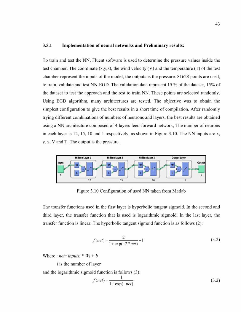
43

3.5.1 Implementation of neural networks and Preliminary results:

To train and test the NN, Fluent software is used to determine the pressure values inside the

test chamber. The coordinate (x,y,z), the wind velocity (V) and the temperature (T) of the test

chamber represent the inputs of the model, the outputs is the pressure. 81628 points are used,

to train, validate and test NN-EGD. The validation data represent 15 % of the dataset, 15% of

the dataset to test the approach and the rest to train NN. These points are selected randomly.

Using EGD algorithm, many architectures are tested. The objective was to obtain the

simplest configuration to give the best results in a short time of compilation. After randomly

trying different combinations of numbers of neutrons and layers, the best results are obtained

using a NN architecture composed of 4 layers feed-forward network, The number of neurons

in each layer is 12, 15, 10 and 1 respectively, as shown in Figure 3.10. The NN inputs are x,

y, z, V and T. The output is the pressure.

Figure 3.10 Configuration of used NN taken from Matlab

The transfer functions used in the first layer is hyperbolic tangent sigmoid. In the second and

third layer, the transfer function that is used is logarithmic sigmoid. In the last layer, the

transfer function is linear. The hyperbolic tangent sigmoid function is as follows (2):

(3.2)

Where : net=inputsi * Wi + b

i is the number of layer

and the logarithmic sigmoid function is follows (3):

(3.2)

2( ) 1

1 exp( 2* )f net

net= −

+ −

1( )

1 exp( )f net

net=

+ −

44

The optimal architecture obtained using the EGD algorithm and obtaining the best results is

composed of 4 layers feed-forward network. The NN-EGD are implemented in Matlab.

To test the approach, we used 14440 points, the Figure 3.12 to Figure 3.14 presents an

example of pressure value for measuring points in the plane 1, 2 and 11 shown in Figure

3.11. The average error of the obtained results in plans 1 is equal to 7.22 %. In the plane 2,

the error is 4.42% and the error in the plane 10 is equal to 3.16 % of the theoretic pressure.

Figure 3.11 Full mesh of ATR42 profile

Figure 3.12 Comparison of pressure theoretic and pressure predict for plane 1

45



3.6 Conclusion

In this work, a new optimization algorithm was used to optimize the number of neurons used

in our network prediction. A dataset of 14440 points chosen randomly from the total dataset

obtained using Fluent software. By using this approach we can successfully obtain the value

of the pressure in each point of the dataset according to the coordinates of each point, the

wind speed and temperature of the test chamber.

.

CHAPTER 4

ARTICLE 2: A HYBRID ORIGINAL APPROACH FOR PREDICTION OF THE AERODYNAMIC COEFFICIENTS OF AN ATR-42 SCALED WING MODEL

Abdallah Ben Mosbah, Ruxandra Botez, and Thien-My Dao



This article was published in Chinese Journal of Aeronautics,

vol. 29, no 1, p. 41-52, 2016

Résumé

Une nouvelle approche pour la prédiction des coefficients de portance, de traînée et de

moments de tangage est présentée. Cette approche a été basée sur une méthode des machines

à vecteurs de support (SVM) et sur un algorithme méta-heuristique d'optimisation appelé

grand déluge étendu (EGD). La nouveauté de cette approche est l'hybridation entre le SVM

et l'algorithme EGD. L'EGD a été utilisé pour optimiser les paramètres de SVM.

L'apprentissage et la validation de cette nouvelle approche ont été réalisés à l'aide des

coefficients aérodynamiques d'un modèle d'aile ATR-42. Les coefficients aérodynamiques

ont été obtenus à l'aide du code XFoil et des essais expérimentaux en utilisant la soufflerie

Price-Païdoussis. Les coefficients obtenus avec notre approche ont été comparés à ceux

obtenus à l'aide du code XFoil et aussi aux coefficients obtenus expérimentalement pour des

différents angles d'attaque et des différents nombres de Mach. Le but principal de cette

méthodologie est d'estimer rapidement les coefficients aérodynamiques des l'aéronefs.

Abstract

To determine flight parameters in real time, a control system was proposed. A new approach

for the prediction of lift, drag, and moment coefficients is presented. This approach is based

48

on the support vector machines (SVM) methodology and an optimization meta-heuristic

algorithm called extended great deluge (EGD). The novelty of this approach is the

hybridization between the SVM and the EGD algorithm. The EGD is used to optimize the

SVM parameters. The training and validation of this new identification approach is realized

using the aerodynamic coefficients of an ATR-42 wing model. The aerodynamic coefficients

data are obtained with the XFoil software and experimental tests using the Price-Païdoussis

wind tunnel. The predicted results with our approach are compared with those from the XFoil

software and experimental results for different flight cases of angles of attack and Mach

numbers. The main purpose of this methodology is to rapidly predict aircraft aerodynamic

coefficients.

4.1 Introduction

For a long time, researchers in artificial intelligence have worked into machines

programming in order to perform different tasks. Different areas have been treated, such as

decision support, pattern recognition, control, robotics, and prediction. However, the

programming of machines that can adapt to all situations and constraints is difficult. For this

reason, research has been done in machine learning. Supervised learning is a technique in

which rules are automatically generated from a database. This learning database is

characterized by a pair of inputs-outputs (xn,yn), where yn= f(xn). The objective of a

supervised learning method is to determine a representation of the function f, called

''prediction function h''. This new function h provides an output y’=h(x’) for a new input x’.

There are two types of problems that may be solved by means of ''supervised learning''. The

first type is a ''regression problem'', in which the output associated with an input is a real

number. The second type is a ''classification problem'', in which the output has a finite

cardinal, and where a label should be assigned to a given input (El Asli, 2008). In this work,

a prediction model is presented to solve a regression problem. To solve this type of problem,

many supervised learning methods can be used, such as neural networks (NNs), fuzzy logic,

and support vector machines (SVMs). These three methods can be applied to conceive

49

prediction or identification models. NNs and fuzzy logic have been used extensively to solve

control systems problems in the aerospace field.

Neural networks have been used in multiple domains, including pattern classification,

optimal control, and manufacturing (Hunt et al., 1992), (Udo, 1992), (Wong et al., 1997),

(Wong et al., 2000), (Chen and Burrell, 2002), in the reliability field by Nourelfath and

Nahas (2003 and 2005) and by Ren and Bai (2011). In aerospace engineering, NNs can be

applied to a large range of complex problems, as presented by Faller and Schreck (1996).

Other problems were resolved using the NN method, such as: the detection and identification

of structural damage (Hebert et al., 1993), helicopter design (Lu et al., 2006), composite

structural optimization (Xu et al., 2005), modeling of aerodynamic characteristics from flight

data (Linse and Stengel, 1993 ), (Sajid et al., 1997), the detection of unanticipated effects

such as icing (Johnson and Rokhsaz, 2001), (Rahmi et al., 2005), and autopilot controllers

and advanced control laws for carefree maneuvering (Napolitano and Kincheloe 1995),

(Ilkay et al., 2001), as well as aerodynamic lift CL and drag CD coefficients prediction

(Wallach et al., 2006). An experimental study on the use of smart sensing and neural

networks to strain loads for different airflow cases were presented by Abha et al. (2000),

where the authors used a fiber-optic sensor to train and verify the neural network

performance. They also used a multilayer network to map the inputs and outputs of a

nonlinear system, thereby to create a three-layered neural network, with three neurons in the

first layer, five in the second layer, and one neuron in the third layer. A hyperbolic tangent

sigmoid function was used in the first and second layers, while a linear function was used in

the third layer. The network was developed through ''supervised learning'', in which

parameters were adjusted to achieve the target outputs for given inputs. Scott and Pado

(2000) developed an adaptive neural network-based control system that integrated three

developed and tested control systems. One system used flutter suppression control laws, a

second system employed a predictive NN control scheme, and a third system used an NN in

an inverse model control scheme. Suresh et al. (2003) used recurrent neural networks for the

prediction of lift coefficients at high angles of attack. In their approach, the lift coefficients

were obtained from wind tunnel tests.

50

Haiping et al. (2007) evaluated the air speed, the angle of attack, and the angle of sideslip in

the control of flying bodies. They have proposed a new experimental methodology by which

the flight parameters were inferred from multiple hot-film flow speed sensors mounted on the

surface of the wing of a micro air vehicle (MAV). In order to obtain a good mathematical

relationship between the sensor readings and the flight parameters, they proposed the use of

micro hot-film flow speed sensor arrays and a back-propagation neural network to determine

the following three flight parameters: air speed, angle of attack, and angle of sideslip

(Haiping et al., 2007 ). Peyada and Ghosh (2009) proposed the feed forward neural networks

method to estimate aircraft parameters from flight data. This method used feed forward

neural networks to establish a neural model that was used to predict the time histories of

motion variables at the (k + 1)th time instant, where the measured initial conditions

corresponded to the kth time instant (Peyada and Ghosh, 2009). A neural network based on a

flush air data sensing system and demonstrated on a mini air vehicle was presented by Samy

et al., (2010).

Xuan et al., (2010) presented a fuzzy neural network controller, which had the advantages of

both fuzzy control and neural network methods. In this method, the uncertain parameters

were controlled for nonlinear time-varying systems. Fuzzy logic can be used to model highly

non-linear, multidimensional systems, including those with variations of parameters, or

where the sensors’ signals were not accurate enough for other models (Sivanandam et al.,

2007). De Jesus Mota and Botez (2009) proposed a new technique for helicopter model

identification from flight test data based on neural networks. The dynamics behavior of a

helicopter was identified with a recurrence method, and an optimization procedure was based

on the neural network theory and tuning of the initial conditions (De Jesus Mota and Botez,

2009). An aeroservoelastic model was presented by Boely and Botez (2010) and by Boely, et

al. (2011), in which neural network and fuzzy logic algorithms identified the multi-input and

multi-output systems of an F/A-18 aircraft. An approach has been proposed by Roudbari and

Saghafi (2014) to identify the dynamics of fighter aircraft using NNs.

51

A flight parameter control system based on neural networks has been proposed by Ben

Mosbah et al. (2013), in which the proposed NNs were optimized using a meta-heuristic

algorithm, called the extended great deluge (EDG). Their approach predicted pressure

distributions and aerodynamic coefficients from the known parameters (angle of attack,

Mach number, etc.). Kouba et al. (2009 and 2010) proposed an identification model, based

on fuzzy logic methods, to identify the nonlinear aircraft models for a high number of flight

tests; their model was used for an F/A-18 aircraft. A new method for the realization of two

neuro-fuzzy controllers for a morphing wing design application was also presented by

Grigorie and Botez (2009) The proposed controllers’ main function had the aim to correlate

each set of pressure differences that were calculated between the optimized and reference

wing airfoils, where each of the airfoil deformations was produced by the actuators’ system

(Grigorie et al., 2009). Several other authors also used fuzzy logic in identification and

control areas (Grigorie and Botez, 2009), (Grigorie et al., 2011), (Grigorie et al., 2012).

4.2 Support vector machines (SVM)

Although the SVM method is specific to classification problems, it can be used in regression

problems. The objective is to determine a representation h(x) in R, called ''estimation

function'' of the original function f(x) given in the learning phase.

The function h(x) is estimated based on a training set of n samples. A tube of width ε is

defined around the desired outputs, so that all the predicted values should be inside this tube.

For a linear regression, the function h(x) is estimated as follows (Cornuejols et al., 2002):

(4.1)

where ω is the weight of the inputs space and b is a threshold ϵ R.

As described by Vapnik (1999), considering a set of data x1, x2,..., xn with targets values

y1, y2,..., yn, the optimization of the prediction function h(x) in the larger space is

characterized by the resolution of the following system (El Asli, 2008):

( )h x wx b= +

52

2 *

1

1min ( )

2

n

i ii

w C ζ ζ=

+ + (4.2)

subject to:

(4.2.1)

(4.2.2)

(4.2.3)

where C is a regularization parameter, which can control the influence of the error, the term

is used to control the complexity of the regression function, ɛ is the width of the tube

defined around the desired outputs, and are the variations of samples which are outside

of the ε-tube (Vojislav, 2001).

For a generalization of a non-linear regression, a kernel function K(x, xi) is used. We use a

Lagrangian function, where the Lagrangian is defined as the sum of the objective function

and a linear combination of constraints whose coefficients (ai ≥ 0) are called Lagrange

multipliers (El Asli, 2008).

As explained by Smola and Schölkopf, (2004), by introducing Lagrange multipliers, our

optimization problem defined in Equation (4.2) becomes a dual form. The shape of the

''regression function'' is defined as follows (Cornuejols et al., 2002): y' = ∑ α . K(x . x) + b∈

(4.3)

where ai and ai* (0 ≤ ai , ai

* ≤ C) are the Lagrange multipliers, which are calculated in the

training process. b is calculated using the constraints of the optimization model (Equation

(4.2)).

The constraint given in Equation(4.2.1) becomes equality using ζi =0 if 0 ˂ ai ˂ C , and the

constraint given in Equation(4.2.2) becomes equality using ζi*=0 if 0 ˂ ai *˂ C. n is the subset

1,2,...,i i iy wx b i nε ζ− − ≤ + ∀ =

* 1, 2,...,i i iwx b y i nε ζ+ − ≤ + ∀ =

*, 0 1, 2,...,i i i nζ ζ ≥ ∀ =

21

2w

*,i iζ ζ

*

1

( ) ( ) ( )n

i i ii

h x a a K x x b=

= − − +

53

of samples corresponding for the nonzero Lagrange multipliers, and K is the kernel function

representing a scalar product in the re-description space.

A kernel function is used to construct the decision surface ''hyper-plan'' in the input space.

Some examples of kernel functions are presented as follows (El Asli, 2008):

The linear kernel function is given by:

K(x, x’) = x. x’ (4.4)

The polynomial kernel function is given by:

K(x, x’) = (x. x’) (4.5)

where d is the degree of the kernel function K

The Gaussian kernel function is given by:

(4.6)

4.3 Optimization of the SVM parameters

For a good functioning of SVM and for obtaining good results, it is essential to use the

appropriate SVM parameters to solve the investigated problem. To choose the SVM

parameters such as C, ε, and the degree d of the kernel function K, it is important to use an

optimization algorithm.

To optimize these parameters, different techniques have been proposed. For example, a

technique has been used by Keerthi (2002) to the tuning of SVM parameters using

radius/margin bound, which is taken as the index to be minimized (Keerthi, 2002).

Cherkassky and Ma (2004) optimized the parameters C and ε when a Gaussian kernel

function was selected using an analytical method. The meta-heuristic methods were also used

to optimize the SVM parameters, such as the simulated annealing algorithm used by Pai and

Hong (2005) to find the best values of C and ε parameters.

2

2

'( , ') exp

2

x xK x x

σ −

= −

54

Since the quality of results necessarily depends on the quality of the SVM parameters, an

original hybridization of the SVM method with a meta-heuristic algorithm is proposed. The

proposed meta-heuristic algorithm is the EGD algorithm used to optimize the SVM

parameters. The EGD algorithm is described in the following section.

4.4 Extended great deluge algorithm

The EGD is a local search procedure that was introduced by Dueck in 1993, and is classified

as a meta-heuristic algorithm. This local search algorithm can accept sometimes bad

solutions whose values are smaller than a certain limit B. This flexibility allows the

optimization of a process to get out of the local minimum. The limit B decreases

monotonically (in the case of minimization problems) during the search. The initial value of

B is equal to the "objective function", and for each iteration, its value decreases by a fixed ΔB

in ''minimization" problems, and increases by the same value of ΔB for "maximization"

problems. The ΔB step represents an ''input parameter'' in this approach. During the search, B

is the limit between a feasible and a non-feasible area of research, and serves to orientate the

solution of the problem towards the ''feasible area''. In other words, the neighborhood of the

solution S* is cut by the limit B and the research is only conducted in one side, below or

above the limit B, depending on the minimization or maximization of the objective function.

The increase or decrease of B with ΔB can be considered as a control process giving a desired

solution. In the beginning phases of research, the solution has the ability to move in both

directions, and can also be found inside the feasible portion limited by B. Otherwise, there is

a great chance of accepting poor solutions, because the limit B is located at a long distance

from the chosen solution S* and a small part of its neighborhood may be cut off. During the

search, the limit B moves closer to the value of the current solution, so the search space

becomes smaller and the possibility of improving the solution becomes lower, leading to the

end of the process research (Dueck, 1993).

The first application completed with this approach was the optimization of an exam timetable

problem that was treated by Burke et al. (2004). The results proved the effectiveness of this

55

algorithm (Ben Mosbah and Dao, 2011). Several of these results have been improved using

approaches such as ''taboos search''.

Figure 4.1 shows the steps of the EGD algorithm (Ben Mosbah and Dao, 2011). This

algorithm was used to resolve a preventive maintenance optimization problem for multi-state

systems by Nahas et al. (2008). The proposed model consisted in finding an optimal

sequence of maintenance actions which minimized maintenance costs (Nahas et al., 2008).

Other applications of the EGD algorithm consisted in the optimization of the scheduling

problems of manufacturing cells as proposed by Ben Mosbah and Dao (2010, 2011 and

2013) and by Ben Mosbah (2011). In these applications, the EGD algorithm gave better

results than the genetic algorithm (GA) and the simulated annealing (SA).

The advantage of the EGD is that only one parameter needs to be adjusted, ΔB, which is

already defined by Burke et al. (2004) have shown that the convergence time of the

algorithm is dependent on the ΔB value. Indeed, an increase of the ΔB value would result in a

decrease of the convergence time, but the quality of solutions could also degrade, which

explains the importance of choosing the best ΔB to obtain a good compromise between

quality of results and calculation time. The EGD algorithm is a meta-heuristic type in which

the optimum solution is not guaranteed, because the search process is based on a randomly

selected initial solution, which is the initial boundary B and the value of ΔB (Ben Mosbah et

al., 2013).

As shown in Figure 4.1, the steps of the EGD algorithm are the following:

Step 1. Choose randomly the initial solution S and ΔB.

Step 2. Calculate the efficiency of S, which is α(S), and assign its value to B.

Step 3. Define the neighborhood N(S) of S.

Step 4. Select randomly a neighboring solution S* belonging to N(S).

Step 5. Compare the new solution N(S*) with the previous solution, N(S) and B.

If two conditions (α(S*) ≤ α(S) and α(S*) ≤ B) are not satisfied, select a new neighboring

solution S;

If one of these conditions is true, then accept the solution S=S* and recalculate B=B ΔB; −

56

Step 6. If the stopping criterion is true, end of process.

Step 7. Else, a new neighboring solution S is selected and the algorithm is tested again (Ben

Mosbah and Dao, 2013).

Figure 4.1 Extended great deluge algorithm Take from Ben Mosbah and Dao (2011)

no

ok

no ok

start

Initialize: ∆B, S

B←α(S)

Calculate the efficiency of S,

α(S)

Define the neighborhood N

(S)

Accept S* and put S=S*

B= B-∆B

END

Select randomly a neighboring

solution S* ϵ N(S)

α(S*) ≤α(S) or

α(S*) ≤ B

Stopping criterion

57

The performance and the results obtained with our proposed algorithm are further evaluated

to determine the lift, drag, and moment coefficients for different angles of attack and Mach

numbers and to compare their values with Xfoil values.

4.5 New proposed SVM-EGD algorithm

In this paper, a hybrid SVM-EGD algorithm is proposed to calculate the lift, drag, and

moment coefficients for different flight cases (angles of attack and Mach number values).

The steps of this hybrid approach are shown in Figure 4.2. In our new algorithm, we use a

qualitative performance measure describing the learning abilities of a given trained SVM

method, in which the training error is expressed as the mean sum of the squared residuals

(the mean squared error (MSE)) in the training data (Pai and Hong, 2005):

(4.7)

where y(xk) is the desired value, y*(xk) is the estimated output of the SVM method for the kth

input xk, and n is the number of data points used in the training set.

As shown in Figure 4.2, the steps of the SVM-EGD approach are the following:

Step 1. Choose randomly the initial parameters S of SVM and ΔB, the initial error, and the

iteration number.

Step 2. Define learning vectors and assign the value of the initial error to B.

Step 3. Define the neighborhood N of S.

Step 4. Select randomly a neighboring solution S* belonging to N(S).

Step 5. Learning of SVM using parameters S* and return the predicted vector y*.

Step 6. Calculate the error between the desired values and the predicted values.

Step 7. Compare the new solution N(S*) with the old solution, N(S) and B:

If two conditions (MSE(S*) ≤ MSE(S) and MSE(S*) ≤ B) are not satisfied, select a new

neighboring solution S.

If one of these conditions is true, then accept the solution S=S*.

[ ]21MSE ( ) * ( )k k

k n

y x y xn ∈

= −

58

Step 8. If the iteration number is reached, end of the process, and keep the optimized

parameters to be used for new input data.

Step 9. Else, recalculate B=B ΔB and go to step 3.

4.6 Infrastructure

In this section, the infrastructure used in the experimental tests is presented. This

infrastructure includes a Price-Païdoussis wind tunnel, a Regional Transport Aircraft ATR-42

model, a fastening system, and a transducer. The infrastructure is used at the Research

Laboratory in Active Controls, Avionics and Aeroservoelasticity (LARCASE).

4.6.1 Price-Païdoussis wind tunnel

The proposed approach is validated using experimental tests carried out in the Price-

Païdoussis subsonic blow-down wind tunnel of LARCASE that is shown in Figure 4.3. This

subsonic wind tunnel has two test chambers: one with a section equal to 0.3 0.6 m2 that

provides a speed up to 60 m/s, and the other with a section of 0.6 0.9 m2 that provides a

speed up to 40 m/s (Ben Mosbah et al., 2013).

Figure 4.2 Price-Païdoussis wind tunnel

−

×

×

Test chamber

59

Figure 4.3 Hybrid SVM-EGD algorithm Taken from Ben Mosbah et al. (2014)

ok

B MSE_int

Initialize SVM parameters S, ΔB, number of iteration and MSE_int

Learning vectors: inputs x and outputs y

Start

MSE(S*)

Output vector y*

Define the neighborhood N

Select randomly a neighboring solution S*

Learning using S*

New input data

SVM-parameters optimized and selected

predicted outputs y_pred with SVM EGD

no

ok

MSE (S*) ≤ MSE (S) Or MSE (S*) ≤ B

no

Accept solution S=S*

B=B- ΔBIteration number?

60

4.6.2 Transducer

During the experimental tests, a ''six-axis force/torque sensor system'' is used to determine

the values of aerodynamic lift CL, drag CD, and moment CM coefficients. The transducer used

in the experiments is a compact and robust structure that converts force and torque into

analog strain gage signals. Through the strain gauges and high quality silicon used in the

design, this sensor can withstand high overload. Figure 4.4 shows the transducer with a

standard tool adapter. The fastening system of the ATR-42 model and the transducer are

shown in Figure 4.5. The assembly consisting of the sensor and the fastening system is

mounted below the test chamber of the wind tunnel.

Figure 4.4 Transducer

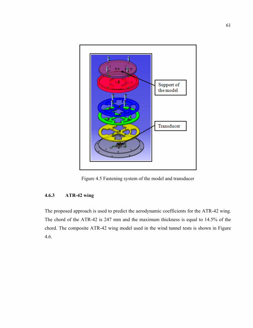
61

Figure 4.5 Fastening system of the model and transducer

4.6.3 ATR-42 wing

The proposed approach is used to predict the aerodynamic coefficients for the ATR-42 wing.

The chord of the ATR-42 is 247 mm and the maximum thickness is equal to 14.5% of the

chord. The composite ATR-42 wing model used in the wind tunnel tests is shown in Figure

4.6.

62

Figure 4.6 ATR-42 model installed in the test chamber of the wind tunnel

4.7 Implementation of the SVM-EGD algorithm and analysis of results

4.7.1 Theoretical results

The aerodynamic lift CL, drag CD, and moment CM coefficients are determined in this paper

for different values of Mach numbers and angles of attack on the ATR-42 model.

For the ''learning'' of the SVM algorithm, a database obtained using Xfoil software was used.

A total of 101 values of lift CL, drag CD, and moment CM coefficients for combinations of

angles of attack between 5o to 5o (0.1o per step) and a Mach number = 0.11 (40 m/s) were

used. These test cases were selected so that they could be validated using the Price-

Païdoussis wind tunnel. The validation data set was composed of 11 random vectors and the

test data set was composed of 11 random vectors.

−

63

The optimal values of the SVM parameters (degree d of the kernel, C, and Ɛ) were obtained

using the EGD algorithm. The Gaussian kernel (Equation(6)) gave better results than the

other kernels (Eqs.(4) and (5)) with the parameter d=2. The other parameters are C= 8036518

and Ɛ=9.29 10-6.

The proposed approach was implemented in MATLAB. The process of training and

optimization of the SVM parameters takes approximately 9 h. Then, the results for these 11

cases are obtained rapidly. The aerodynamic lift CL, drag CD, and moment CM coefficients

values are presented in Tables 4.1-4.3 and in Figures. 4.7-4.9, for a number of 11 flight cases

expressed in terms of angles of attack's and Mach numbers.

Table 4.1 Original versus predicted lift coefficients for different airflow cases.

Alpha Mach number

Original lift

coefficient

(XFoil)(10-2)

Predicted lift

coefficient (SVM-

EGD) (10-2)

MSE (10-4)

4.7

0.11

26.76 27.08

0,037

3.6 15.62 15.53 2.7 6.54 6.56 2 0.78 0.84

1.3 8.14 7.94 0.1 19.8 19.82

0.6 26.48 26.32 1.6 36.4 36.4 2.6 46.84 46.79 3.9 61.76 61.42

4.7 72.19 72.52

×

− − −− − −− − −−

−−

64

Figure 4.7 Lift coefficient CL versus angle of attack

Table 4.2 Original versus predicted drag coefficients for different airflow cases.

Alpha Mach number Original drag

coefficient (XFoil)(10-3)

Predicted Drag coefficient (SVM-

EGD)(10-3)

MSE(10-6)

4.7

0.11

11.01 11.03

0,00055

3.6 10.82 10.84 2.7 10.82 10.84 2 10.65 10.64

1.3 10.41 10.46 0.1 9.25 9.23

0.6 8.77 8.76 1.6 8.63 8.66 2.6 9.05 9.04 3.9 9.73 9.71 4.7 10.18 10.2

−−−−

−−

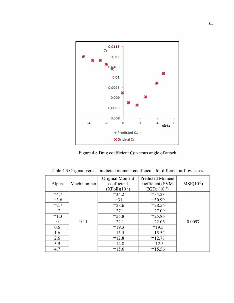
65

Figure 4.8 Drag coefficient CD versus angle of attack

Table 4.3 Original versus predicted moment coefficients for different airflow cases.

Alpha Mach numberOriginal Moment

coefficient (XFoil)(10-3)

Predicted Moment coefficient (SVM-

EGD) (10-3)

MSE(10-6)

4.7

0.11

34.2 34.28

0,0097

3.6 31 30.99 2.7 28.6 28.56 2 27.1 27.09

1.3 25.8 25.86 0.1 22.1 22.06

0.6 19.3 19.3 1.6 15.5 15.54 2.6 12.8 12.78 3.9 12.8 12.5 4.7 15.6 15.56

− − −− − −− − −− − −

− − −− − −

− −− −− −− −− −

66

Figure 4.9 Moment coefficient CM versus angle of attack

4.7.2 Experimental results

The experimental results using the Price-Païdoussis wind tunnel are presented. For the

''learning'' of the SVM, a database obtained using experimental tests was used. A total of 100

values of lift (CL), drag (CD), and moment (CM) aerodynamic coefficients for combinations of

angles of attack Alpha between 9o to 15o (1o per step) and Mach numbers of 0.058, 0.073,

0.088, and 0.117 were used, for the Reynolds numbers of 316666, 395833, 475000, and

633333, respectively.

The learning of the SVM approach was done using 60 flight cases, and was tested using 40

flight cases randomly selected from the database. The computing time for the training and

testing of the SVM algorithm was calculated using the optimal values of the SVM parameters

(degree d=2 of the Gaussian kernel, C= 8036518, and Ɛ=9.29 10-6) and took less than 1

second to obtain CL, CD, and CM for the 40 flight cases. The experimental and predicted

SVM-EGD results are presented in Tables 4.4-4.6 and in Figures 4.10-4.12. Table 4.4 and

−

×

67

Figure 4.10 show the lift coefficient CL variation with Alpha angle of attack, Table 4.5 and

Figure 4.11 present the drag coefficient CD variation with Alpha angle of attack, while the

moment coefficient CM variation with Alpha angle of attack are presented in Table 4.6 and

Figure 4.12.

68

Table 4.4 Experimental versus predicted lift coefficients for different airflow cases.

Alpha Mach number

Experimental lift coefficient

(10-2)

Predicted lift coefficient (SVM-EGD) (10-2)

9

0.058

30.14 19.21 6 16.1 15.02 3 1.18 0.12 2 3.94 4.72

0 12.75 12.4 3 27.32 27.22 7 51.7 50.53 9 62.33 61.66 12 76.61 76.49 14 89.65 90.29

9

0.073

29.63 18.59 6 15.57 14.96 3 1.35 0.6 2 4.25 4.26

0 13.05 13.71 3 26.85 26.79 7 50.38 47.86 9 59.33 60.63 12 77.46 75.03 14 88.17 88.85

9

0.088

29.51 19 6 15.8 14.67 3 1.67 0.17 2 4.33 4.8

0 13.19 13.42 3 27.21 27.28 7 48.31 48.19 9 58.75 58.9 12 75.07 74.32 14 88.39 87.27

9

0.117

43.77 19.47 6 15.57 14.8 3 1.62 0.13 2 4.42 4.79

0 13.48 13.36 3 27.77 28.09 7 47.66 47.77 9 57.87 57.08 12 72.7 72.8 14 82.98 85.77

− − −− − −− −−

− − −− − −− −−

− − −− − −− −−

− − −− − −− −−

69

Figure 4.10 Lift aerodynamic coefficients variation versus angle of attack

70

Table 4.5 Experimental versus predicted drag coefficients for different airflow cases.

Alpha Mach number Experimental drag coefficient

(10-2)

Predicted drag coefficient

(SVM-EGD) (10-2)

9

0.058

4.03 4.11 6 2.50 2.83 3 2.50 1.92 2 1.68 1.92

0 1.97 2.05 3 2.62 1.92 7 4.15 4.67 9 5.61 5.89 12 8.73 8.05 14 10.78 10.74

9

0.073

3.55 3.65 6 2.35 2.62 3 2.37 1.94 2 1.67 1.93

0 1.95 1.91 3 2.49 1.82 7 4.07 4.52 9 5.41 5.91 12 8.69 7.85 14 10.67 10.61

9

0.088

3.30 3.49 6 2.15 2.48 3 2.27 1.82 2 1.60 1.87

0 1.87 1.85 3 2.51 1.83 7 4.01 4.43 9 5.35 5.71 12 8.48 7.82 14 10.81 10.50

9

0.117

2.98 3.11 6 1.99 2.24 3 2.04 1.64 2 1.56 1.70

0 1.82 1.75 3 2.44 1.88 7 3.94 4.40 9 5.41 5.65 12 8.99 8.49 14 4.20 6.53

−−−−

−−−−

−−−−

−−−−

71

Figure 4.11 Drag aerodynamic coefficients variation versus angle of attack

72

Table 4.6 Experimental versus predicted moment coefficients for different airflow cases.

Alpha Mach number

Experimental moment coefficient (10-2)

Predicted moment coefficient (SVM-EGD) (10-2)

9

0.058

12.84 10.16 6 9.04 8.85 3 3.57 3.92 2 2.85 2.47

0 0 0.11 3 4.52 4.32 7 10.23 10.01 9 12.61 12.73 12 16.41 16.1 14 19.27 19.49 -9

0.073

-12.94 -9.94 -6 -8.83 -8.61 -3 -3.65 -4.25 -2 -2.89 -2.79 0 -0.15 -0.09 3 4.26 4.3 7 10.05 9.68 9 12.18 12.6 12 16.44 16.03 14 19.03 19.14

9

0.088

12.9 9.74 6 8.88 8.59 3 3.7 4.3 2 2.85 2.85

0 0.11 0.18 3 4.23 4.19 7 9.83 9.89 9 12.26 12.51 12 15.86 15.73 14 19.13 18.98

9

0.117

13.32 10.09 6 8.8 8.54 3 3.75 4.3 2 2.91 2.82

0 0.18 0.13 3 4.16 4.16 7 9.93 9.89 9 12.49 12.44 12 15.94 16.07 14 18.37 19.08

− − −− − −− − −− − −

−

− − −− − −− − −− − −

− −

− − −− − −− − −− − −

− −

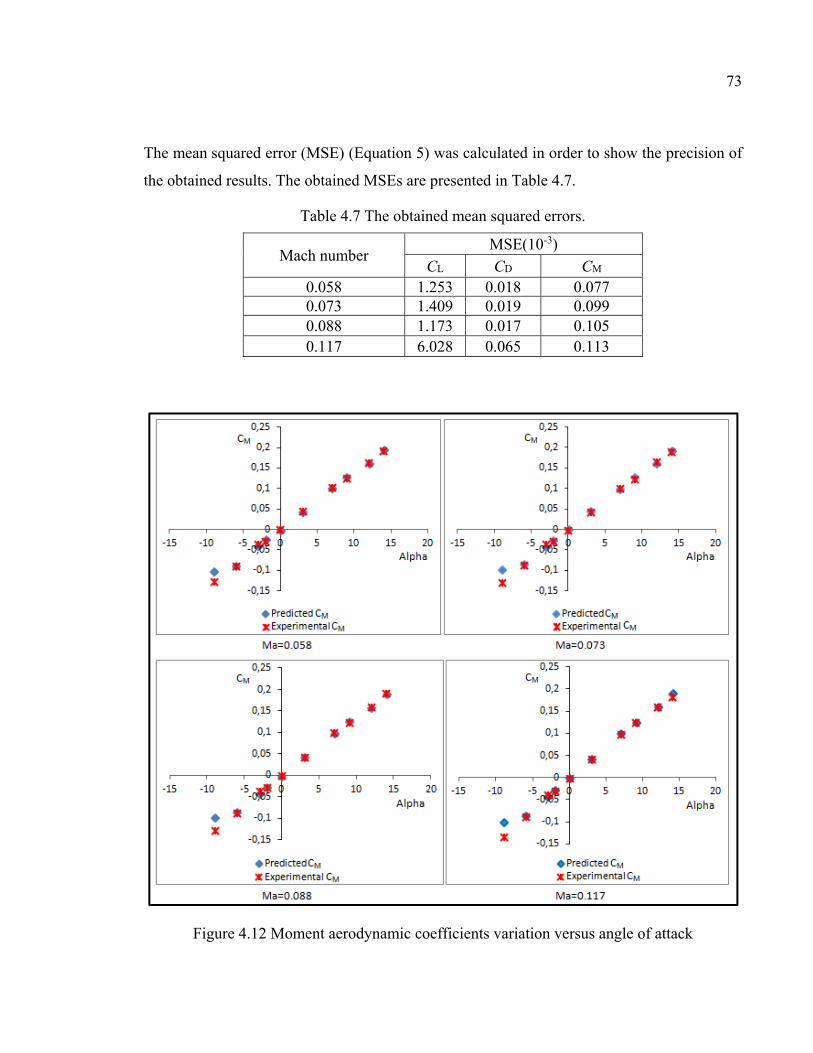
73

The mean squared error (MSE) (Equation 5) was calculated in order to show the precision of

the obtained results. The obtained MSEs are presented in Table 4.7.

Table 4.7 The obtained mean squared errors.

Mach number MSE(10-3)

CL CD CM 0.058 1.253 0.018 0.077 0.073 1.409 0.019 0.099 0.088 1.173 0.017 0.105 0.117 6.028 0.065 0.113

Figure 4.12 Moment aerodynamic coefficients variation versus angle of attack

74

4.8 Conclusions

(1) A new algorithm using the SVM-EGD approach was used to optimize the values of the

SVM parameters by use of the EGD approach. The proposed approach is used to predict

aircraft aerodynamic coefficients for different flight cases.

(2) The obtained results were validated using experimental wind tunnel tests. Since the

mean squared errors between the predicted and the experimental results are very low

where the fitted line is very close to desired data, we conclude that the SVM-EGD

approach is robust and accurate. In addition, the mean squared errors for the results

obtained with XFoil versus those from SVM-EGD are almost zero, where the MSE

does not exceed a maximum of 0.03 10-4 for the lift coefficient, of 0.55 10-9 for the

drag coefficient, and 0.97 10-8 for the moment coefficients.

× ×

×

CHAPTER 5

ARTICLE 3: NEW METHODOLOGY COMBINING NEURAL NETWORK AND EXTENDED GREAT DELUGE ALGORITHMS FOR THE ATR-42 WING

AERODYNAMICS ANALYSIS

Abdallah Ben Mosbah, Ruxandra Botez, and Thien-My Dao



This article was published in The Aeronautical Journal,

vol. 120, nº 1229. pp. 1049-1080

Résumé

La détermination rapide des paramètres aérodynamiques tels que la distribution de pression,

la portance, la traînée et le moment de tangage a partir des conditions d'écoulement connues

(l'angle d'attaque, le nombre de Mach et le nombre Reynolds) en temps réel est toujours

difficile à réaliser par des méthodes d'analyse numérique en aérodynamique et en

aéroélasticité. Un système de contrôle des paramètres de vol a été proposé pour résoudre ce

problème. Ce système de contrôle est basé sur de nouvelles méthodologies d'optimisation à

l'aide des réseaux de neurones (NNs) et de l'algorithme de grand déluge étendu (EGD).

La validation de ces nouvelles méthodes est réalisée par des tests expérimentaux sur un

modèle d'aile d'avion installé dans une soufflerie équipée de trois systèmes de mesure

différents (un capteur FlowKinetics, un capteur AEROLAB PTA et un manomètre avec

plusieurs tubes) pour déterminer la répartition de la pression. En ce qui concerne les

coefficients de la portance, de la traînée et du moment de tangage, ceux obtenus par notre

approche sont comparés avec ceux obtenus à l'aide du code de calcul aérodynamique XFoil et

aussi avec les coefficients expérimentaux obtenus pour différents angles d'attaque et nombres

de Mach. Le but principal de ce nouveau système de contrôle est d'améliorer la performance

76

aérodynamique de l'aile et de l'appliquer pour améliorer les performances aérodynamiques

des avions.

Abstract

The fast determination of aerodynamic parameters such as pressure distributions, lift, drag

and moment coefficients from the known airflow conditions (angles of attack, Mach and

Reynolds numbers) in real time is still not easily achievable by numerical analysis methods

in aerodynamics and aeroelasticity. A flight parameters control system is proposed to solve

this problem. This control system is based on new optimization methodologies using neural

networks (NNs) and extended great deluge (EGD) algorithms. Validation of these new

methodologies is realised by experimental tests using a wing model installed in a wind

tunnel, and 3 different transducer systems (a FlowKinetics transducer, an AEROLAB PTA

transducer and Multitube Manometer tubes) to determine the pressure distribution. For lift,

drag and moment coefficients, the results of our approach are compared to the XFoil

aerodynamics software and the experimental results for different angles of attack and Mach

number. The main purpose of this new proposed control system is to improve, in this paper,

wing aerodynamic performance, and, in future to apply it to improve aircraft aerodynamic

performance.

5.1 Introduction and background

The ability to predict the parameters of various air loads on an airplane is very useful in

aircraft design. The precise determination of aerodynamic parameters such as pressure

distributions and aerodynamic coefficients (lift, drag and moment) from known parameters

such as angles of attack, Mach and Reynolds numbers in real time is still not rapidly

achieved by numerical analysis aerodynamics methods. The numerical results are usually

validated by experimental tests in wind tunnels or in flight.

77

Control systems are used to control the air on a wind tunnel model, usually of reduced scale,

by using various control methodologies incorporating modern sensors and actuators. These

methods use various optimization techniques (Neural Network, Fuzzy Logic, Extended Great

Deluge ...). The tests were performed in the Price-Païdoussis subsonic blow down wind

tunnel at the Research Laboratory in Active Controls, Avionics and

Aeroservoelasticity (LARCASE). This wind tunnel has two test chambers; the first chamber

has a 1x2 ft section that provides maximum speed of 60 m/s, and the second chamber has a

2x3 ft section that works for maximum speed of 40 m/s.

Neural networks (NNs) have been used in multiple domains, including pattern classification,

optimal control, and manufacturing (Wong et al., 2000), (Hunt et al., 1992), (Udo et al.,

1992), (Wong et al., 1997), (Chen and Burrell, 2002). Applications of NNs in the field of

reliability have been proposed by Nourelfath and Nahas (2003 and 2005), and by Ren and

Bai (2011). A model based on NNs and fuzzy min-max was proposed by Seera et al. (2012)

to detect and classify the comprehensive fault conditions of induction motors. In Aerospace

Engineering, NNs can be applied to a large range of complex problems, as shown in (Faller

and Schreck, 1996). Neural networks have been used to solve many problems in the

aeronautical industry, such as: the detection and identification of structural damage (Hebert

et al., 1993), the modeling of aerodynamic characteristics from flight data (Linse and

Stengel, 1993), (Sajid et al., 1997), the detection of unanticipated effects such as icing

(Johnson and Rokhsaz, 2000), (Johnson and Rokhsaz, 2001), (Rahmi et al., 2005), autopilot

controllers and advanced control laws for applications such as carefree maneuvering

(Napolitano and Kincheloe, 1995), (Ilkay et al., 2001), as well as lift and drag aerodynamic

coefficients CL and CD prediction (Wallach et al., 2006).

In 2000, researchers began to use neural network techniques in wind tunnels in the aerospace

field, mainly to design control systems. Abha et al. (2000) presented an experimental study

for the use of smart sensing and Neural Networks applied to strain loads for different airflow

cases. They have used a fiber-optic sensor to train and verify the neural network performance

78

and incorporated a multilayer network to map the inputs and the outputs for a nonlinear

system. They used a neural network consisting of three layers; the first layer contained 3

neurons, the second layer contained 5 neurons, and the third one contained 1 neuron. A

''hyperbolic tangent sigmoid function'' was used in the first, and in the second layer; in the

third layer, the ''linear function'' was employed. The network was developed through

''supervised learning'' in which parameters were adjusted to achieve the target outputs for

given inputs. In particular, a back-propagation algorithm was used to minimize the error

between the desired output and the current network output. The principle of this algorithm

was to provide input to the network, and then, by forward propagation, to calculate the output

obtained from the network. The error was calculated for the output, and the error contribution

of each neuron was further estimated. Then, by using the ''steepest gradient algorithm'', the

weights and bias’ of each neuron were updated to minimize the error (Abha et al., 2000).

In 2000, Scott and Pado (2000) developed an adaptive neural network-based control system.

Three control systems were developed and tested in their work. The first system was used for

flutter design, and for validation of suppression control laws, the second system employed a

predictive NN control scheme, and the third system used a neural network in an inverse

model control scheme. The author described some of the methodologies and results obtained

in the Adaptive Neural Control of Aeroelastic Response (ANCAR) project. The goal was to

develop and demonstrate control systems using the Benchmark Active Controls Technology

(BACT) wind-tunnel model.

Suresh et al. (2003) used recurrent neural networks for the prediction of lift coefficients at a

high angle of attack. In their approach, the lift coefficient was obtained from the wind tunnel

test. Haiping et al. (2007) considered the air speed, the angle of attack and the angle of

sideslip fundamental parameters in the control of flying bodies. They proposed a new

experimental methodology by which the flight parameters were inferred from multiple hot-

film flow speed sensors mounted on the surface of the wing of a Micro Air Vehicle (MAV).

To obtain a good mathematical relationship between the readings of the sensors and the flight

parameters they proposed micro hot-film flow speed sensor arrays and a back-propagation

79

neural network to determine three flight parameters: air speed, angle of attack and angle of

sideslip (Haiping et al., 2007).

Peyada and Ghosh, (2009) proposed using Feed Forward Neural Networks to estimate

aircraft parameters from flight data. That method used Feed Forward Neural Networks to

establish a neural model able to predict the time histories of motion variables at the (k + 1)th

instant, given that the measured initial conditions correspond to the kth instant (Peyada and

Ghosh, 2009).

A neural network based on a flush air data sensing system and demonstrated on a mini air

vehicle was presented by Samy et al. (2010). A new active fault tolerant control strategy was

proposed by Yuying et al. (2010) for the system in the presence of actuator fault and input

constraints, utilizing neural networks to approximate the plant uncertainty and the adaptive

parameters, adjusted with a projection algorithm (Yuying et al., 2010). Xuan et al. (2010)

presented a fuzzy neural network controller, which had the advantages of both fuzzy control

and neural networks, for the control of uncertain parameters for nonlinear time-varying

systems.

Neural network structures have several advantages. For example, they employ a highly

parallel structure if networks with a larger number of hidden layers are used. All the neurons

in a layer can be computed simultaneously to enhance the speed. Another advantage is the

simplicity of the required computations performed by each neuron of the network.

Fuzzy logic can be used to model highly nonlinear, multidimensional systems, including

those with parameter variations, or where the sensors’ signals are not accurate enough for

other models (Sivanandam et al., 2007). De Jesus-Mota and Botez (2009) proposed a new

technique for helicopter model identification from flight data tests based on neural networks.

The dynamics behavior of the helicopter was identified with a recurrence method and an

optimization procedure based on neural network theory and the tuning of the initial

80

conditions (De Jesus-Mota and Botez, 2009). An aeroservoelastic model was presented by

Boely and Botez (2010), Boely et al. (2011), in which neural network and fuzzy logic

algorithms identify the multi-input and the multi-output system of an F/A-18 aircraft.

Many numerical and meta-heuristic algorithms have been proposed for the optimization and

training of NN models, such as genetic algorithm, extended great deluge, and simulated

annealing. A numerical algorithm was proposed by Zhang (2006) for training feed-forward

neural networks using a recursive prediction error method (Zhang, 2006). A flight parameter

control system based on neural networks was proposed by Ben Mosbah et al. (2013), in

which the proposed NNs are optimized using a meta-heuristic algorithm, called the extended

great deluge (EDG). Their approach predicted pressure distributions and aerodynamic

coefficients from the known parameters (angles of attack, Mach numbers, Reynolds numbers,

etc.). Xiao et al. (2012) proposed a fault tolerant altitude tracking control scheme for flexible

spacecraft with a partial loss of actuator effectiveness fault. In their proposed model, NNs are

integrated to approximate the unknown system dynamics. An approach to identify and model

the dynamics of fighter aircraft using NNs was proposed by Roudbari and Saghafi (2014).

NNs have also been applied in the design field. Lu et al. (2006) proposed a hybrid approach

for helicopter design based on genetic algorithms and NNs. An approach based on the

genetic algorithm and NNs was proposed by Xu et al. (2005), and was further applied to

replace the currently-deployed expensive finite element analysis during composite structural

optimization (Xu et al., 2005).

Kouba et al. (2009 and 2010) proposed an identification model, based on fuzzy logic

methods, to identify nonlinear aircraft models for many flight test cases; their proposed

model was applied for an F/A-18 aircraft. A study presented by Grigorie et al. (2009)

described a new method for the realization of two neuro-fuzzy controllers for a morphing

wing design application. Their proposed system correlated each set of pressure differences,

calculated between the optimized and the reference airfoil, with each of the airfoil

deformations produced by the actuators. Piroozan (2005) proposed an intelligent control

81

system that used electro-optics and neural networks to control the flow of air over a flexible

wall. A study presented by Panigrahi et al. (2003) predicted the turbulence statistics behind a

square cylinder using neural networks and fuzzy logic. An improved neural network-based

method was proposed by Voitcu and Wong (2003) to predict the nonlinear oscillations in the

aeroelastic response. A neural network model was used by Shuhui Li et al. (2014) to control

a grid-connected rectifier/inverter. Several other uses of fuzzy logic have been presented by

the same authors in identification and control areas (Grigorie and Botez, 2009 and 2011),

(Grigorie et al., 2011 and 2012).

5.2 Flight parameters

The main objective in this section is to determine the influence of the Mach number Ma and

the angle of attack α around an airfoil. For the learning and validation of the NN-EGD, the

results were obtained by use of the wind tunnel of the Research Laboratory in Active

Controls, Avionics and Aeroservoelasticity (LARCASE). Using XFoil aerodynamics

software, the distribution of pressure coefficients (Cp) was obtained around the airfoil for an

ATR-42 reduced-scale wing model.

The distribution of the total pressure P was obtained using the well-known aerodynamics

formula (Equation 5.1):

(5.1)

The Reynolds number (Re) and Mach (Ma) number were calculated using the following

formulas (Equations 5.2 and 5.3):

(5.2)

(5.3)

where L is the characteristic length linear dimension (m), V is the air velocity (m/s), is

the kinematic viscosity (m²/s) and a is the sound speed.

21

2PP C U Pρ∞ ∞ ∞ = ∗ ∗ ∗ +

e

V LR

ν∗=

VMach

a=

82

Another objective is to determine the drag (CD), lift (CL) and moment (CM) coefficients for

different values of the air speed and angles of attack for an ATR-42 airfoil. To learn and test

our approach, XFoil code was used to obtain their values.

5.3 XFOIL code

In This study, XFoil 6.96 was used to obtain aerodynamic coefficient for an ATR-42 airfoil.

This bi-dimensional aerodynamic analysis code is developed by Drela and Giles in 1987. It

used to analyze and draw aerodynamic airfoils. The aerodynamic analysis using XFoil gives

a good prediction of the laminar/turbulence transition resulting of the precision of drag and

lift calculation. This performance was proved by experimental tests performed by Helge and

Antonino (1995). Authors tested and proved that XFoil code gives a acceptable aerodynamic

coefficients regarding to the experimental results in cruise flight angle of attack for subsonic

airfoil analysis (Daniel et al., 2010).

For the viscose/inviscid calculation, different methods were used in XFoil. The inviscid

analysis are performed using a linear vorticity stream function panel method. To perform a

good prediction, a Karman-Tsien compressibility correction is added to XFoil. For viscose

calculation, the method was used for the boundary layer and wake formulations (Daniel et

al., 2010).

The XFoil code is faster than other CFD software, which is useful to be connected with an

optimization process of morphing airfoils. However, the obtained results using XFoil cannot

match exactly the wind tunnel results due to the three-dimensional flow effects (Daniel et al.,

2010).

5.4 Neural networks

Neural Networks have been used in different domains, especially in aerospace. Some

applications of neural networks are aircraft component fault detectors, autopilot

83

enhancements, flight path simulations, and aircraft control systems. They have also been

proposed to control flight parameters.

Artificial neural networks are mathematical models inspired from biological neurons; they

can reproduce an artificial intelligent reasoning. Neural networks are one of the most

important components of the field of artificial intelligence. An artificial neural network is a

processing structure which employs a massively parallel architecture. It is built up of

interconnected simple processing units or neurons. Each neuron passes on a weighted

function of its inputs to the next layer of neurons (Abha et al., 2000). A general structure of

one neuron is shown in Figure 5.1. Neural networks have many inputs (x1 x2 ... xn), outputs

(yi), and linearity or/and nonlinearity in their transfer functions. The function of each neuron

is to sum the weighted inputs (wi,j) and the bias (bj) and process this sum through a transfer

function (f) (Scott and Pado, 2000). This function (f) can be linear ( = ∑ , + ) or

non-linear (for example: the tan-sigmoid transfer function = Tanh(∑ , + ).

Figure 5.1 Architecture of an artificial neuron

84

5.5 EXTENDED GREAT DELUGE

In this work, an optimization algorithm based on the meta-heuristic Extended Great Deluge

(EGD) is used. This algorithm was presented by Burke et al. (2004), and the first application

realized with this approach was the optimization of the exam timetable problem treated by

Burke et al., (2004). Several of their results have been improved using approaches such as

''taboos search''. Figure 5.2 shows the steps of the EGD algorithm (Burke et al., 2004). This

algorithm was used to solve a preventive maintenance optimization problem for multi-state

systems by Nahas et al. (2008). Their model found an optimal sequence of maintenance

actions that minimized maintenance costs (Nahas et al., 2008). Another application of the

EGD algorithm was the optimization of the group scheduling problem by Ben Mosbah and

Dao (2010 and 2011) (two of the authors of this paper), in which the EGD algorithm gave

better results than a genetic algorithm (GA) and simulated annealing (SA).

The EGD algorithm has not yet been used in aerospace problems. Based on its strong

performance, this algorithm was used in hybridization with neural networks to find the

predicted flight parameters. As explained by Burke et al., (2004), the EGD is a local search

procedure introduced by Dueck (1993). This algorithm works as Simulated Annealing (SA)

but it accepts solutions that are poorer than those from SA to identify the local minimum.

The first step of the algorithm, as shown in Figure 5.2, consists of randomly initializing ΔB

and the initial value of the SVM parameters (S). Next, the efficiency α (the Error) of S is

calculated, and its value is assigned to B. The neighborhood N(S) of S is then defined; a

neighboring solution S* belonging to N(S) is randomly selected; and the new solution N(S*) is

compared with the old solution, N(S) and B. If the two conditions (α(S*)≤ α(S) and B) are not

satisfied, then a new neighboring solution S is selected; if one of these conditions is true, then

the solution S* is accepted, and B=B-ΔB is recalculated. Finally, the stopping criterion is

tested, and if the number of iterations has been reached, the algorithm ends. A new

neighboring solution S is selected and the algorithm is tested again (Ben Mosbah and Dao,

2013).

85

In this work, a hybrid NN-EGD method is proposed to control the pressure distribution, as

well as the lift, drag and moment coefficients by varying the angles of attack at low Reynolds

numbers.

Figure 5.2 General flowchart of the EGD algorithm Taken from Ben Mosbah and Dao (2011)

86

5.6 NN-EGD ALGORITHM

The EGD algorithm is used to obtain the optimal network configuration so that the output

error would be as small as possible. The different steps of the approach are presented in

Figure 5.3. Qualitative performance measures are used to describe the learning abilities of

given trained neural networks. The training error is defined as the mean sum of the squared

residuals (mean squared error (MSE)) of the training data, as follows (Equation 5.4):

(5.4)

where ti is the desired value, yi is the estimated output of the recurrent neural networks and N

is the number of data points used by the training set.

It is necessary to specify the type of neighborhood in which the EGD algorithm needs to be

adjusted, as shown in Figure 5.2, applied to an optimization NN problem. The research is

based on an iteratively feasible solution to another conducted to find a solution to the

problem by performing changes in motions in the neighborhood. During the optimization

process, the number of neurons is restricted to 15 neurons per layer. The NN parameters are

chosen and the algorithm is performed as follows:

1) Number of layers = 1

2) Random selection of a number of neurons between 1 and 15

3) Training and testing of the network

4) Number of layers =Number of layers + 1

5) One layer is chosen randomly and go to step 2) if the number of iterations has not

been reached.

21Error ( )i i

i N

t yN ∈

= −

87

5.7 Implementation of NN-EGD and theoretical results

In this study, two prediction systems are proposed, both based on neural networks. The first

(NNPred_1) is used to predict the lift (CL), the drag (CD) and the moment coefficients (CM), and

the second (NNPred_2) is used to predict the pressure coefficients (Cp). The inputs parameters

for these prediction systems are the angles of attack and the Mach numbers. These systems

are described in Figure 5.4.

88

Figure 5.3 Proposed algorithm

89

Figure 5.4 Predictions systems

5.7.1 The CL, CD and CM prediction system

The lift (CL), drag (CD) and moment (CM) coefficients are obtained with XFoil to ''train'' and

''test'' the NN-EGD_pred1 given in Figure 5.4. A number of 101 combinations of angles of

attack α between -5o to 5o (0.1o per step), and Mach number = 0.1 (Reynolds number was

539470) were used. The validation data set and the test data set were around 20% of the

database, corresponding to 11 random vectors were used for each.

The optimal architecture obtained using the EGD algorithm is composed of a four- layer

feed-forward network. The number of neurons and the transfer functions are presented in

Table 5.1.

The scheme of the neural networks used to predict aerodynamic coefficients is illustrated in

Figure 5.5.

Table 5.1 Neural network architecture for CL, CD and CM prediction

Layer number Number of neurons Transfer function

1 12 Logarithmic sigmoid 2 8 Hyperbolic tangent sigmoid 3 9 Logarithmic sigmoid 4 3 Linear

α

Mach number

Chord

NN-EGD_pred1

NN-EGD_pred2 CP

CL, CD and CM

90

Let O(k) represent the outputs of layer k, the general formula to calculate the outputs O(k) is as

follows (Equation 5.5):

Figure 5.5 Neural Network architecture for the NN-EGD_pred1 model

For layer 1, the transfer function is logarithmic sigmoid and the outputs O(1) are calculated

using the following equation (Equation 5.6):

( ) = × , + × , + ℎ × , + (5.6) = 11 + −( × , + × , + ℎ × , + )

j =1...12 (number of neurons in layer 1)

For layer 2, the transfer function is hyperbolic tangent sigmoid and the outputs O(2) are

calculated as follows (Equation 5.7):

( ) = ∑ ( ) , + (5.5)

where: f is the transfer function;

j is the index of neurons in the layer (k);

n is the number of the neurons in the layer (k-1); and

i is the index of neurons in the layer (k-1).

91

( ) = ∑ ( ) × , + (5.7) = 21 + −2 ∑ ( ) × , + − 1


For layer 3, the transfer function is logarithmic sigmoid and the outputs O(3) are determined

as follows (Equation 5.8): ( ) = ∑ ( ) × , + (5.8) = 11 + ∑ ( ) × , +


Layer 4 represents the output layer and O(4) is a vector equal to (CL, CD, CM); the transfer

function used in this layer is linear and the equations of CL, CD, CM are as follows (Equation

5.9):

( ) = = ∑ ( ) × , + (5.9)

= , , … ,, , … ,, , … , ⋮ +

The NN-EGD are implemented in MATLAB. The obtained results are presented in Figures

5.6 to 5.8 and Tables 5.2 to 5.4.

92

Table 5.2 Lift coefficients variation with the angle of attack (XFoil versus NN-EGD results)

Figure 5.6 Lift coefficient versus angle of attack

Table 5.3 Drag coefficients variation with the angle of attack (XFoil versus NN-EGD results)

α -4.5 -4 -3.1 -2.5 -1.5 0 0.5 2 2.8 3.5 4.4

Cl_XFoil -

0.2472 -

0.1964 -

0.1065 -0.0447 0.0603 0.2074 0.2550 0.4053 0.4906 0.5677 0.6819

Cl_NN-EGD

prediction

-0.2474

-0.1964

-0.1065

-0.0447 0.0599 0.2066 0.2557 0.4055 0.4904 0.5663 0.6819

% CL_error

0.0690 0 0 0 0.5995 0.3956 0.2628 0.0578 0.0312 0.2465 0

α -4.5 -4 -3.1 -2.5 -1.5 0 0.5 2 2.8 3.5 4.4 CD_XFoil 0.0110 0.0108 0.0109 0.0108 0.0105 0.0092 0.0088 0.0088 0.0091 0.0095 0.0100 CD_NN-

EGD prediction

0.0109 0.0109 0.0109 0.0107 0.0106 0.0093 0.0088 0.0087 0.0090 0.0095 0.0100

% CD_error

0.4956 0.2077 0.0063 0.4683 0.5563 1.2198 0.2185 0.4640 0.8034 0.5420 0.0207

93

Figure 5.7 Drag coefficient versus angle of attack

Table 5.4 Moment coefficients variation with the angle of attack (XFoil versus NN-EGD results)

α -4.5 -4 -3.1 -2.5 -1.5 0 0.5 2 2.8 3.5 4.4

CM_XFoil -

0.0336 -

0.0322 -

0.0295 -

0.0281 -

0.0261 -

0.0217 -

0.0197 -

0.0143 -

0.0126 -

0.0119 -

0.0143 CM_NN-

EGD prediction

-0.0336

-0.0322

-0.0296

-0.0282

-0.0262

-0.0217

-0.0197

-0.0142

-0.0125

-0.0121

-0.0143

% CM_error

0.0343 0.1221 0.4139 0.4045 0.5536 0.0336 0.1877 0.4621 0.9911 1.9786 0.2516

94

Figure 5.8 Moment coefficient versus angle of attack

The results presented in Figures 5.6 to 5.8 and in Tables 5.2 to 5.4 show the efficiency of the

proposed approach. The error between the obtained values using XFoil and the values

predicted by the proposed neural network was of a very low order. The proposed NN-EGD

method gave very good results as the error percentages for the lift, drag and moment

coefficient did not exceed 0.6 %, 1.2 % and 2%, respectively.

5.7.2 The Cp prediction system

The pressure coefficients CP results used to train and test the NN-EGD_pred2 given in Figure

5.4 were obtained in XFoil for 11 combinations of angles of attack α and Mach numbers. The

angles of attack varied between -5o to 5o (1o per step) and the Mach number was fixed to 0.1,

corresponding to Reynolds number of 539470. The NN-EGD were validated and tested with

2 random angles of attack, α= -2o and α= 3o. The optimal architecture obtained using the

EGD algorithm that gave the best results was composed of a 4-layer feed-forward network.

The number of neurons and the transfer functions are presented in Table 5.5.

95

Table 5.5 Neural network architecture for Cp prediction

Layer number Number of neurons Transfer function

1 10 Hyperbolic tangent sigmoid 2 10 Logarithmic sigmoid 3 10 Hyperbolic tangent sigmoid 4 1 Linear

The scheme of the neural networks used to predict pressure coefficients is illustrated in

Figure 5.9.

Figure 5.9 Neural architecture of the NN_pred2 model

The outputs O(k) of each layer k are calculated similarly as the for the outputs of the

NN_pred1 model. Layer 4 represents the output layer and O(4) is equal to Cp; the pressure

coefficient Cp is calculated as follows (Equations 5.10 to 5.13):

Layer 1: ( ) = × , + × , + ℎ × , + ; = 1. . .10 (5.10)

Layer 2: ( ) = ∑ ( ) × , + ; = 1. . .10 (5.11)

Layer 3: ( ) = ∑ ( ) × , + ; = 1. . .10 (5.12)

Output layer: ( ) = = ∑ ( ) × ( ) + ( ) (5.13)

96

The distributions of the CP on the inner and upper surfaces of the ATR42 wing airfoil are

presented in Figures. 5.10 and 5.11 for two values of angles of attack.

Figure 5.10 Pressure coefficient distribution versus the chord for the angle of attack α=-2o

Figure 5.11 Pressure coefficient distribution versus the chord for the angle of attack α=3o

97

In this test, the average percentage error for the pressure coefficients CP is lower than 5 %,

except at one point on the chord. The experimental results are generally good, as shown in

Figures 5.10 and 5.11.

5.8 Experimental tests

This section presents the numerical results obtained during testing in the Price-Païdoussis

wind tunnel. The goal is to measure the pressures on the upper surface of the airfoil to

determine the pressure coefficients’ distribution and to compare it with the numerical results

obtained with both the XFoil code and the proposed algorithm shown in Figure 5.3.

5.8.1 Equipment

This section presents the Price-Païdoussis wind tunnel, the ATR-42 wing model and the

pressure transducer systems.

The Price-Païdoussis subsonic blow down wind tunnel available at the Research Laboratory

in Active Controls, Avionics and Aeroservoelasticity (LARCASE) (Figure 5.12) was used to

realize the testing and validation of our prediction systems. This subsonic wind tunnel is

equipped with two test chambers; each with its own characteristics and dimensions. The

smaller chamber provides a maximum airspeed of 60 m/s and the larger offers a maximum

airspeed of 40 m/s.

The wing model used in the wind tunnel tests is a reduced scale model of the ATR42 aircraft.

This model was designed and manufactured in the LARCASE laboratory. Figure 5.13(a)

represents a composite aircraft ATR-42 wing model used for wind tunnel tests. The upper

surface wing is covered by distributed pressure taps as shown in Figure 5.13(b). The

locations of these taps were pre-defined to ensure an optimal observation of the changes in

the Cp distribution given by the XFoil code. Figure 5.14 represents the airfoil of the ATR 42

model.

98


Figure 5.13 Model of the composite wing ATR-42

99

Figure 5.14 Airfoil of the ATR-42 wing

During these wind tunnel tests, for experimental validation purposes, three pressure

transducers were used to measure the pressure distribution around the ATR-42 airfoil. The

first system was the FlowKinetics transducer; in this transducer, the pressure measurements

were obtained at each port, as shown in Figure 5.13(b), and were made one at a time, because

this transducer was equipped with three sensors of different precisions.

The second transducer was a Pressure Transducer Array (PTA) produced by AEROLAB.

This system was equipped with 24 pressure transducer channels to measure the pressure at

the same time on all 14 taps on the wing airfoil.

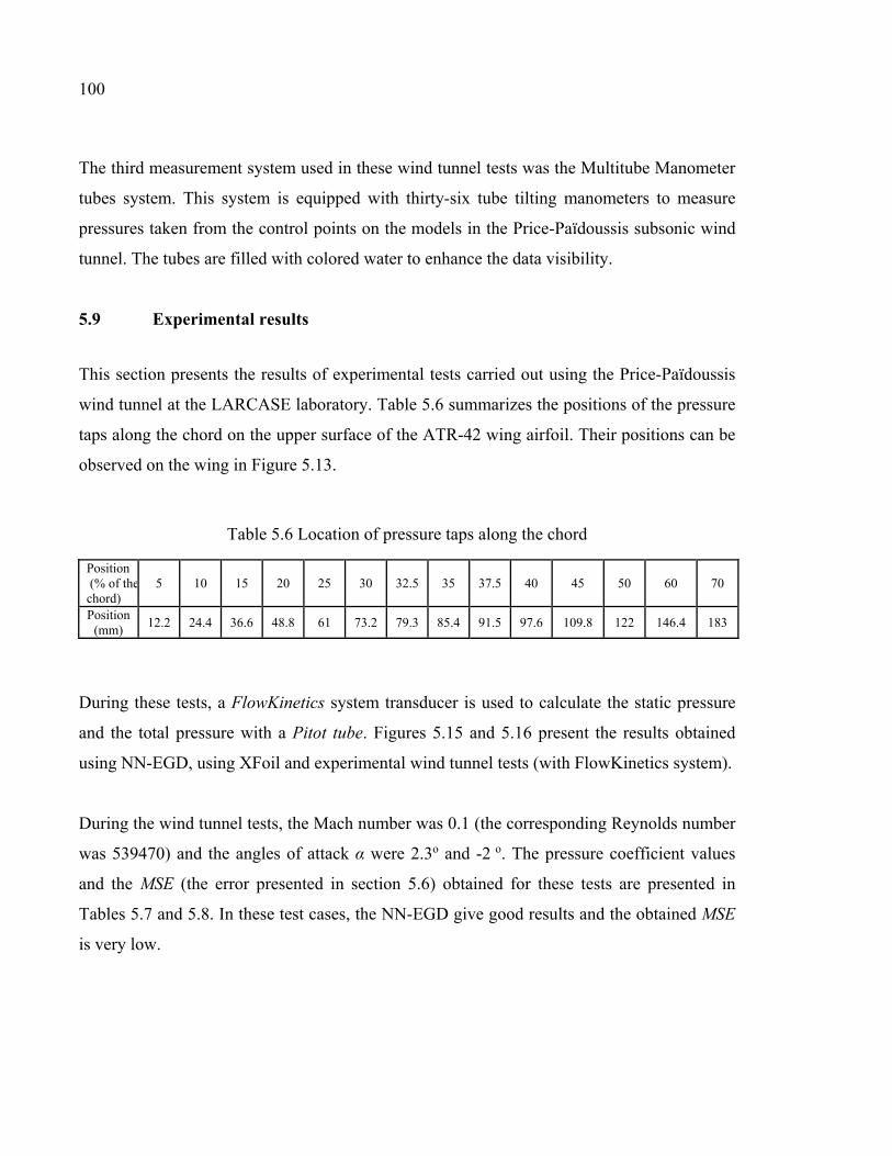
100

The third measurement system used in these wind tunnel tests was the Multitube Manometer

tubes system. This system is equipped with thirty-six tube tilting manometers to measure

pressures taken from the control points on the models in the Price-Païdoussis subsonic wind

tunnel. The tubes are filled with colored water to enhance the data visibility.

5.9 Experimental results

This section presents the results of experimental tests carried out using the Price-Païdoussis

wind tunnel at the LARCASE laboratory. Table 5.6 summarizes the positions of the pressure

taps along the chord on the upper surface of the ATR-42 wing airfoil. Their positions can be

observed on the wing in Figure 5.13.

Table 5.6 Location of pressure taps along the chord

During these tests, a FlowKinetics system transducer is used to calculate the static pressure

and the total pressure with a Pitot tube. Figures 5.15 and 5.16 present the results obtained

using NN-EGD, using XFoil and experimental wind tunnel tests (with FlowKinetics system).

During the wind tunnel tests, the Mach number was 0.1 (the corresponding Reynolds number

was 539470) and the angles of attack α were 2.3o and -2 o. The pressure coefficient values

and the MSE (the error presented in section 5.6) obtained for these tests are presented in

Tables 5.7 and 5.8. In these test cases, the NN-EGD give good results and the obtained MSE

is very low.

Position (% of thechord)

5 10 15 20 25 30 32.5 35 37.5 40 45 50 60 70

Position (mm)

12.2 24.4 36.6 48.8 61 73.2 79.3 85.4 91.5 97.6 109.8 122 146.4 183

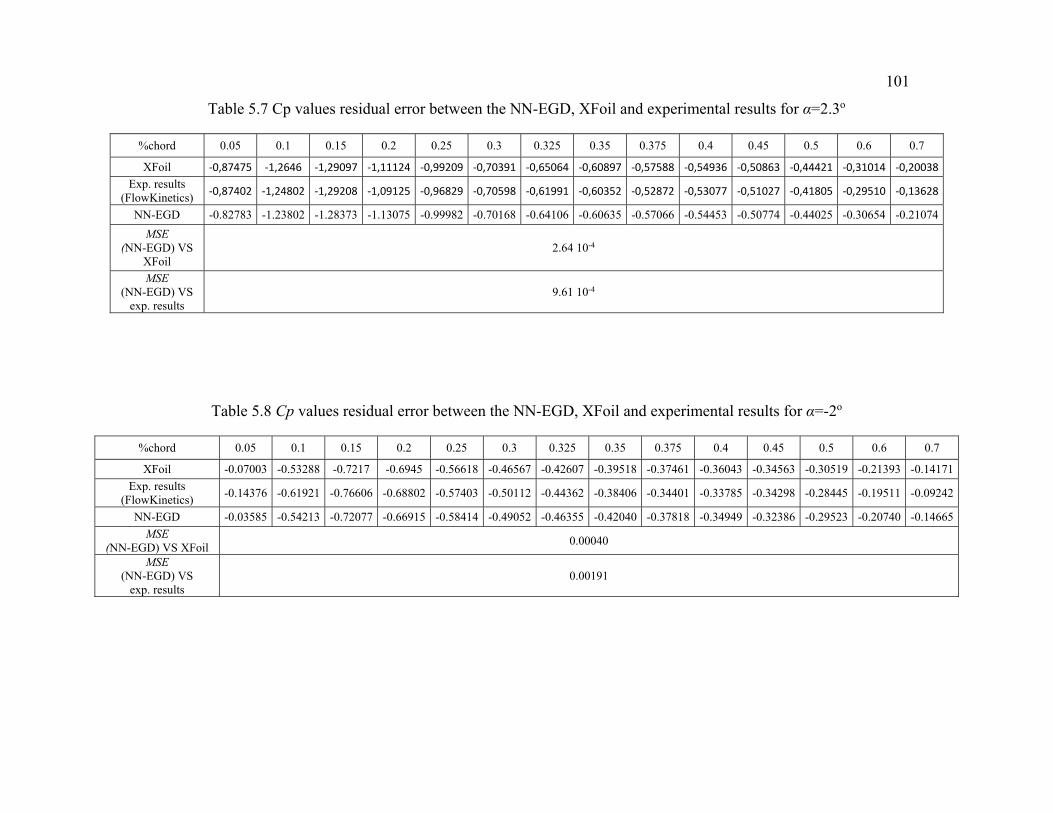
101

Table 5.7 Cp values residual error between the NN-EGD, XFoil and experimental results for α=2.3o

%chord 0.05 0.1 0.15 0.2 0.25 0.3 0.325 0.35 0.375 0.4 0.45 0.5 0.6 0.7

XFoil -0,87475 -1,2646 -1,29097 -1,11124 -0,99209 -0,70391 -0,65064 -0,60897 -0,57588 -0,54936 -0,50863 -0,44421 -0,31014 -0,20038Exp. results

(FlowKinetics) -0,87402 -1,24802 -1,29208 -1,09125 -0,96829 -0,70598 -0,61991 -0,60352 -0,52872 -0,53077 -0,51027 -0,41805 -0,29510 -0,13628

NN-EGD -0.82783 -1.23802 -1.28373 -1.13075 -0.99982 -0.70168 -0.64106 -0.60635 -0.57066 -0.54453 -0.50774 -0.44025 -0.30654 -0.21074

MSE (NN-EGD) VS

XFoil 2.64 10-4

MSE (NN-EGD) VS

exp. results 9.61 10-4

Table 5.8 Cp values residual error between the NN-EGD, XFoil and experimental results for α=-2o

%chord 0.05 0.1 0.15 0.2 0.25 0.3 0.325 0.35 0.375 0.4 0.45 0.5 0.6 0.7

XFoil -0.07003 -0.53288 -0.7217 -0.6945 -0.56618 -0.46567 -0.42607 -0.39518 -0.37461 -0.36043 -0.34563 -0.30519 -0.21393 -0.14171

Exp. results (FlowKinetics)

-0.14376 -0.61921 -0.76606 -0.68802 -0.57403 -0.50112 -0.44362 -0.38406 -0.34401 -0.33785 -0.34298 -0.28445 -0.19511 -0.09242

NN-EGD -0.03585 -0.54213 -0.72077 -0.66915 -0.58414 -0.49052 -0.46355 -0.42040 -0.37818 -0.34949 -0.32386 -0.29523 -0.20740 -0.14665

MSE (NN-EGD) VS XFoil

0.00040

MSE (NN-EGD) VS

exp. results 0.00191

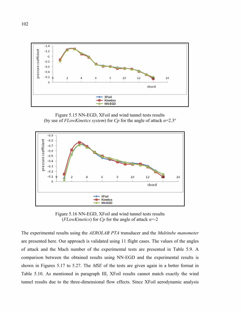
102

Figure 5.15 NN-EGD, XFoil and wind tunnel tests results (by use of FLowKinetics system) for Cp for the angle of attack α=2.3o

Figure 5.16 NN-EGD, XFoil and wind tunnel tests results (FLowKinetics) for Cp for the angle of attack α=-2

The experimental results using the AEROLAB PTA transducer and the Multitube manometer

are presented here. Our approach is validated using 11 flight cases. The values of the angles

of attack and the Mach number of the experimental tests are presented in Table 5.9. A

comparison between the obtained results using NN-EGD and the experimental results is

shown in Figures 5.17 to 5.27. The MSE of the tests are given again in a better format in

Table 5.10. As mentioned in paragraph III, XFoil results cannot match exactly the wind

tunnel results due to the three-dimensional flow effects. Since XFoil aerodynamic analysis

103

were used to train NN-EGD approach, it is possible to have a little difference between Price-

Païdoussis wind tunnel results and the NN-EGD predicted values, mostly close to the

transition zone, such as shown in Figures 5.20 and 5.21.

Table 5.9 Test parameters

Reynolds number Mach number Angle of attack α

539470 0.1 -2, 0, 1, 2o

485520 0.09 -2, 0, 1, 2o

431573 0.08 -2, 1, 2o

Table 5.10 The residual error between the NN-EGD method and the experimental results

Reynolds number

Mach number α MSE (NN-

EGD_PTA)

MSE (NN-EGD_Multitube

Manometer)

539470 0.1

-2 0.00162542 0.00081125 0 0.00062219 0.00135366 1 0.00086812 0.00156837 2 0.00083031 0.00071968

485520 0.09

-2 0.00083092 0.0005574 0 0.00097804 0.0031611 1 0.00125069 0.00185142 2 0.00095717 0.00093497

431573 0.08 -2 0.00074382 0.00234414 1 0.00193907 0.0022361 2 0.00164107 0.00164107

104

Figure 5.17 NN-EGD and experimental results (PTA & Multitube manometer) of Cp for angle of attack α=0o and Reynolds number=539470

Figure 5.18 NN-EGD and experimental results (PTA & Multitube manometer) of Cp for angle of attack α=0o and Reynolds number =485520


105



106




Figure 5.25 NN-EGD and experimental results (PTA & Multitube manometer) of Cp for angle of attack α=-2o and Reynolds number =539470

107



5.10 Conclusion

This work presents a new combined methodology of neural networks and extended great

deluge methods (NN-EGD) used in network prediction. Different cases were used to test the

performance of the approach; 11 theoretical test cases were used to predict the CD, CL and CM

coefficients, and 2 other tests cases were used to predict pressure coefficients. The theoretical

results were acceptable and they could be further improved. The average percentage error did

not exceed 0.6 % for lift CL, 1.2 % for drag CD and 2% for the moment CM coefficient. The

108

average percentage error for the pressure coefficients CP was lower than 5 %, except for a

few points on the chord. To verify the quality of the pressure coefficients predicted by the

NN-EGD method, the obtained results were compared to 11 experimental test case results.

These experiments were conducted using the Price-Païdoussis subsonic blow down wind

tunnel and the 3 measurement systems at the LARCASE laboratory. The obtained results

were very good and the mean squared error (MSE) did not exceed 3.10-3 for all of the test

cases. Based on these theoretical and experimental tests, the proposed NN-EGD approach

was found to be a good flight parameter prediction system for the ATR42 wing airfoil. Future

research could evaluate the performance of this approach on the morphing ATR-42 wing

airfoil and other airfoils.

CHAPTER 6

ARTICLE 4: A NEURAL NETWORK CONTROLLER FOR ATR-42 MORPHING WING ACTUATION

Abdallah BEN MOSBAH, Ruxandra BOTEZ, Thien My DAO

Mohamed Sadok Guezguez, Mahdi Zaag



This article was published in the scientific journal INCAS BULLETIN,

Vol. 8, Issue 2, 2016

Résumé

Une aile d'avion à peau déformable est utilisée pour améliorer les performances de l'avion.

Pour obtenir les profils souhaités de l'aile, des actionneurs électriques sont utilisés. Ces

actionneurs sont installés à l'intérieur d'une maquette d'aile d'avion ATR-42 pour modifier sa

surface supérieure afin d'obtenir sa forme désirée. Pour atteindre cet objectif, un système de

commande de position est nécessaire. Dans ce travail, la conception et la validation d'un

contrôleur basées sur les réseaux de neurones sont présentées. Deux systèmes composant ce

contrôleur, le premier système est un contrôleur de position et le deuxième système est un

contrôleur de courant pour gérer le courant consommé par les actionneurs électriques afin

d'obtenir leur déplacements souhaités. Le modèle de l'aile a été testé et validé numériquement

ainsi qu'expérimentalement. Les résultats numérique obtenus ont été comparés à ceux

obtenus en utilisant un contrôleur PID. Les tests expérimentaux ont été réalisés dans la

soufflerie Price-Païdoussis au Laboratory of Applied Reasearch in Active Controls, Avionics

and Aeroservoelasticity (LARCASE) pour calculer la répartition de pression sur un modèle

d'aile déformable de l'avion ATR-42 pour des différents cas de vol. Les coefficients de

pression obtenus expérimentalement ont été comparés aux coefficients de pression obtenus

numériquement calculé par le code XFoil.

110

Abstract

A morphing wing model is used to improve aircraft performance. To obtain the

desired airfoils, electrical actuators are used, which are installed inside of a mock-up wing of

an ATR 42 aircraft to modify its upper surface in order to obtain the desired shape. To

achieve this objective, a robust position controller is needed. In proposed research, a design

and test validation of a controller based on neural networks is presented. This controller was

composed by a position controller and a current controller to manage the current consumed

by the electrical actuators to obtain the desired displacement. The model was tested and

validated using simulation and experimental tests. The obtained results using the proposed

controller were compared to the results given by the PID controller. The wind tunnel tests

were conducted in the Price-Païdoussis Wind Tunnel at the LARCASE laboratory in order to

calculate the pressure coefficient distribution on an ATR-42 morphing wing model for

different flow conditions. The pressure coefficients obtained experimentally were compared

with their numerical values given by XFoil software.

6.1 Introduction

To be able to design a morphing wing control system, it is essential to understand the

motivation and the aerodynamic issues (Brossard, 2013). The fuel consumption can be

reduced if the aerodynamic drag is reduced. An efficient way to reduce the drag is to develop

a long laminar boundary layer by geometrical deformation of the airfoil in flight accordingly

with flight conditions. The objective is to delay the flow transition on the upper surface of the

wing (Sainmont, 2009). The ''morphing'' is done with the aim to change one or more parts of

a structure geometry in order to improve its aerodynamic performances (Weisshaar, 2006).

Accordingly to Sofla et al. (2010), ''morphing'' can be achieved to change the geometry along

the chord, the span or the camber of the airplane wing to improve the lift and reduce the drag.

Campanile and Sachau (2000) proposed a method to modify the camber of the wing. Another

concept was used by Chandrasekhara et al., (1997) to adapt the leading edge, while Joel et al.

(2007) presented a compliant structure to change the geometry of the wing trailing edge.

Many other morphing wing studies have been proposed to improve the lift (Baron et al.,

111

2003), (Yang et al., 2006), (Strelec et al., 2003), or to obtain a better laminarity of the flow

(David and Jamey, 2001), (Martins and Catalano, 1997).

The determination of the appropriate airfoil for each flight case was done for an optimization

phase by means of experimental flight tests or using optimization algorithm (Daniel, 2010).

For example, a numerical model based on a genetic algorithm was used by Strelec et al.

(2003) to optimize the shape parameters of an airfoil. For the use of an experimental

optimization method, Joel et al. (2007) proposed an approach to determine the optimal flap

deflections. A genetic algorithm was used by Boria et al. (2009) to optimize a unmanned

morphing wing and to test it in a Wind Tunnel. Their proposed model aimed to maximize the

lift and efficiency by using a wind tunnel (Boria et al., 2009). A multidisciplinary approach

was proposed by Sainmont et al., 2009) to change the morphing upper surface and to

optimize the laminar airfoil.

For the deformation of the wing skin, the use of a reliable and accurate actuation and control

system is necessary to obtain the desired shape determined in the optimization phase. A

closed-loop control system was proposed by Popov et al. (2008 and 2010) to validate a

morphing wing model in a wind tunnel. Another study based on using an open-loop

controller to test a morphing wing was presented by Popov et al. (2010). The same authors

presented the optimization of a morphing wing in real time using wind tunnel validation tests

(Popov et al., 2010). Grigorie et al., (2010 and 2012) have proposed many controllers based

on different techniques; in (Grigorie et al., 2010) they proposed a new control technique

using a combined PI and bi-positional laws optimum for a morphing wing application. An

actuation mechanism and a control technique based on on-off proportional-integral-

controllers were proposed and tested experimentally (Grigorie et al., 2012).

Many other control methods are used extensively in the literature, such as Fuzzy Logic and

Neural Networks (NN). These two methods are also used, alone or in hybridization, to

resolve many other problems, such as classification, optimal control and manufacturing

112

(Wong et al., 2000), (Hunt et al., 1992), (Udo, 1992), (Wong et al, 1997), (Chen, 2002).

These methods are extremely efficient to solve nonlinear and multidimensional systems.

Xuan et al. (2010) proposed a controller of uncertain parameters for nonlinear systems based

on NN and Fuzzy Logic methods. A hybrid fuzzy logic proportional-integral-derivative and a

conventional on-off controller were proposed by Grigorie et al. (2012) for morphing wing

actuation. Two other control applications based on Fuzzy Logic were proposed by the same

authors (Grigorie and Botez, 2009), (Grigorie et al., 2012). Large complex problems in

aerospace engineering have been solved using NNs. Hebert et al. (1993) used NNs to

implement fault detection in aircraft. Models based on NNs techniques are proposed by Linse

and Stengel (1993), Wallach et al. (2006), and Ben Mosbah et al. (2013 and 2014) to identify

and predict aerodynamic coefficients, and other methods for detection and icing

identification were developed in (Johnson and Rokhsaz, 2001) and (Rahmi et al., 2005).

Controllers for autopilot systems based on NNs were developed by Napolitano and

Kincheloe (1995). Ben Mosbah et al. (2013) developed a new hybridization NNs model and

extended the great deluge algorithm; their model was validated using wind tunnel test.

In this study, a control system based on NNs is proposed. The model was designed to be

incorporated in an ATR 42 morphing wing used and validated experimentally during wind

tunnel testing.

6.2 ATR-42 Morphing Wing Model

A mechanism was developed to in order to build an experimental prototype of a morphing

model which will be used in wind tunnel tests. This mechanism consists principally of two

eccentric axes mounted inside the model and animated in rotation by two electric actuators.

The system is used to change the upper surface of the model using the eccentric axes; moved

by its rotation, the axes push the composite skin vertically upwards at 30% and 50% of the

chord to obtain the desired deformation of up to 4 mm. The required amount of force that

needs to be developed by each actuator line on the skin to produce the desired deformation

mainly depends on the composite structure of the skin, including the positions and the

number of the actuators. Daniel (2010) demonstrated that two actuation rows were sufficient

113

to obtain good aerodynamic results for a morphing wing skin equipped with SMAs

(Brossard, 2013). Figure 6.1 shows the ATR-42 morphing wing model assembled with the

deformation skin mechanism and Figure 6.2 shows the profile of the ATR-42 wing model

and the position of the eccentric axes.

Figure 6.1 CAD of the ATR-42 model

Figure 6.2 ATR-42 airfoil

Eccentric axes at 30% and 50% of

the chord

Actuators

ATR-42airfoil

114

6.3 The closed loop architecture of the model

To obtain the desired airfoil shape, we need to deform the skin using two actuators. These

deformations should be as close as possible (equal) experimentally with those determined

numerically; a robust position controller is needed. The two actuators that deform the airfoil

of the model from its original to its desired shape and the architecture of the control scheme

are shown in Figure 6.3.

Figure 6.3 Architecture of the closed loop system control

6.3.1 Controller architecture

As shown in Figure 6.4, the control system is composed of a position controller, a current

controller, a saturation voltage block to protect the motor, and a DC motor block.

A control system based on the Proportional Integral Derivative PID was proposed by

Kammegne Tchatchueng et al. (2014) to control the actuators positions of the ATR-42

morphing wing model (the same model used in this study). The results obtained with the

PID controller were satisfactory, with an error margin of 0.4 %. The concept here is to

replace the PID controller with another controller based on neural networks, for more

precision and comparison purposes between the efficiencies of both controllers. The

''position controller'' bloc and the ''current controller'' bloc shown in Figure 6.4 are replaced

by two NN blocs obtained by the proposed algorithm.

115

Figure 6.4 Closed loop control

6.3.2 Modeling of the DC motor

The deformation of the skin is realized using two DC motors, and in order to obtain the exact

desired deformation, a robust control system should be used. Firstly, the mathematical model

of the motors is identified. The DC motors can be configured using electrical,

electromechanical and mechanical engineering equations (Brossard, 2013). Figure 6.5

represents the DC motors’ armature.

Figure 6.5 Representation of the DC motors

where:

U voltage [V],

116

Rm resistance [Ω],

L inductance [H],

im current [A],

Te torque [N·m],

Em counter-electromotive force.

As described by Brossard (2013) and Kammegne Tchatchueng et al. (2014), the motor

resistance Rm and the inductance are assumed to be constants. The actuator model can be

described by the following equations:

= + + (6.1)

= (6.2)

= (6.3)

= + + (6.4)

where:

Wm motor angular speed [rad/s],

ke angular speed constant [revolution/min/V],

kf friction coefficient [N·m/(rad/s)],

TL load torque [N·m],

J inertia [Kg·m2].

To study the stability of a real system such as that of a DC motor, a Laplace transform must

be applied to switch from the time domain to the frequency domain. The Laplace transform

of Equation (6.1) is the following:

( ) = . ( ) + . . ( ) + . ( ) (6.5)

( ) = ( ) − . ( )+ . (6.6)

117

and the Laplace transform of Equation (6.4) is:

( )− ( ) = . ( ) + . . ( )(6.7)

From where: ( ) = ( )− ( )+ . (6.8)

and by replacing the Laplace transform of Equation (6.3) into Equation (6.8),we obtain:

( ) = + . . (S) − ( )+ . (6.9) Where ''S'' is the Laplace operator.

In the absence of the load torque, i.e., TL=0, by replacing TL=0 into Equation (6.9), the Im(S)

can be written as follows:

( ) = . s + (s) (6.10)

By replacing Im(S) given by Equation (6.10) in Equation (6.5), the motor voltage U(S)

becomes: (s) = ( . s + ) . s + (s) + . (s) (6.11)

The transfer function of the model, by use of Equations (6.9) and (6.11), is:

(s) = (s)(s) = . · s + . + . . s + . + . (6.12)

118

In our morphing wing model of the ATR-42, a Maxon motor is used. The datasheet provided

by the manufacturer includes the internal motor characteristics to calculate the modeling

parameters. These characteristics are presented in Table 6.1.

Table 6.1 Internal Motor Characteristics

Rm [Ω] J [kg.m²] Kt [Nm/A] L [H] Kf [Pa.s]

11.4 65.9e-7 0.119 0.0316 1.01738·10-5

The model has been validated by Brossard (2013) and Kammegne Tchatchueng et al. (2014);

its validation consisted in the comparison of the values of im and wm given by the

manufacturer with simulation values using Matlab/Simulink. The results confirmed that the

model was working well. The obtained values of the motor current and the motor speed were

the same as the values given by the manufacturer.

6.4 Neural Network Control System Design

To design a robust control system, a position controller and a current controller are needed,

as seen in Figure 6.4. These two blocs have a very good performance in order to obtain good

results from the control system. Two Neural Networks are designed to ensure a high

performance level. The first NN is used to control the position, for which where the inputs

are the desired positions in degrees and the output is the needed current. The second neural

network controller is used to control the current consumed by the motor; the input of this

bloc is the current and the output is the voltage required to reach the desired position. Figure

6.6 shows the architecture of our control system, using 2 NN algorithms.

119

Figure 6.6 Control system architecture

Each neural network controller of the ''position controller'' and the ''current controller'',

needs a database. The motor used here works using a current between -3.5A and 3.5A and a

voltage of -48V to 48V. The database for the first NN controller is composed of the desired

position in degrees, and the current for which this position represents the input and the

current represents the output. This database is used to train the neural network; therefore it

can be used to control the current values. The output of the first neural network (the position

controller) is the input of the second (the current controller), as seen on Figure 6.6. For the

training phase of the second neural network, the selected database is composed of the current

values as an input of the current controller, and the output is the voltage value supplied to the

power supply, then to the motor to obtain the desired deformation. The challenges of this

methodology resides in the choice of two databases to obtain the desired deformation of the

morphing wing. The idea is to accelerate the system when errors are important at the

beginning of the simulation and avoid overshooting. Tests are needed to determine the right

120

data. We started the training using linear inputs and outputs. For the first controller, the

inputs values are the error between the desired position and the measured position (-360o to

360o with step equal to 0.18), and the outputs are the current between -3.5A to 3.5A with step

equal to 1.75 10-3. We need to accelerate the system when the measured value is far away

from the desired value. For the second controller, the inputs values are the current between -

3.5A and 3.5A with step equal to 0.01 and the outputs are the voltage between -48V to 48V

with step equal to -0,137. For this objective, different data are testing and the results are

analyzed to define the right interval.

After a few tests, we were able to construct databases that gave good results. Tables 6.2 and

6.3 represent the databases used to train the neural network position controller (Table 6.2 and

Figure 6.7), and the database used to train the neural network current controller (Table 6.3

and Figure 6.8), respectively.

In Table 6.2, for the values of deformation between -360o and -50o, to accelerate the system,

the output current is fixed at -3.5A, and for the deformation values between 50o and 360o, the

current is equal to 3.5A. For the deformation values between -50o and 50o, the current varies

between -3.5A and 3.5A described by the following equation (Figure 6.7):

Current=0.07*position.

Figure 6.7 Used data to train the position controller

121

Table 6.2 ''Position controller'' database

The input: the deformation [degree] The output: the current [A]

-360 degree ˂ deformation ˂ -50 degrees -3.5 A

-50 degree ≤ deformation ≤ 50 degrees 0.07*deformation

50 degree ˂ deformation ˂ 360 degrees 3.5 A

InTable6.3, for the current values between -3.5A and -0.6A, the output voltage value is -48V

and for the current values between 0.6A and 3.5A, the corresponding voltage is equal to 48V.

For the range of current values between -0.6A and 0.6A, the output voltage varies between -

48V and 48V and given by the following expression as follows (Figure 6.8):

Voltage=80*current.

Figure 6.8 Used data to train the current controller

Table 6.3 ''Current controller'' database

The input: the current [A] The output: the voltage[V]

-3.5˂ current˂ -0.6 A -48 V

-0.6 A ≤ current ≤ 0.6 A 80*current

0.6 A ˂ current ˂ 3.5 A 48 V

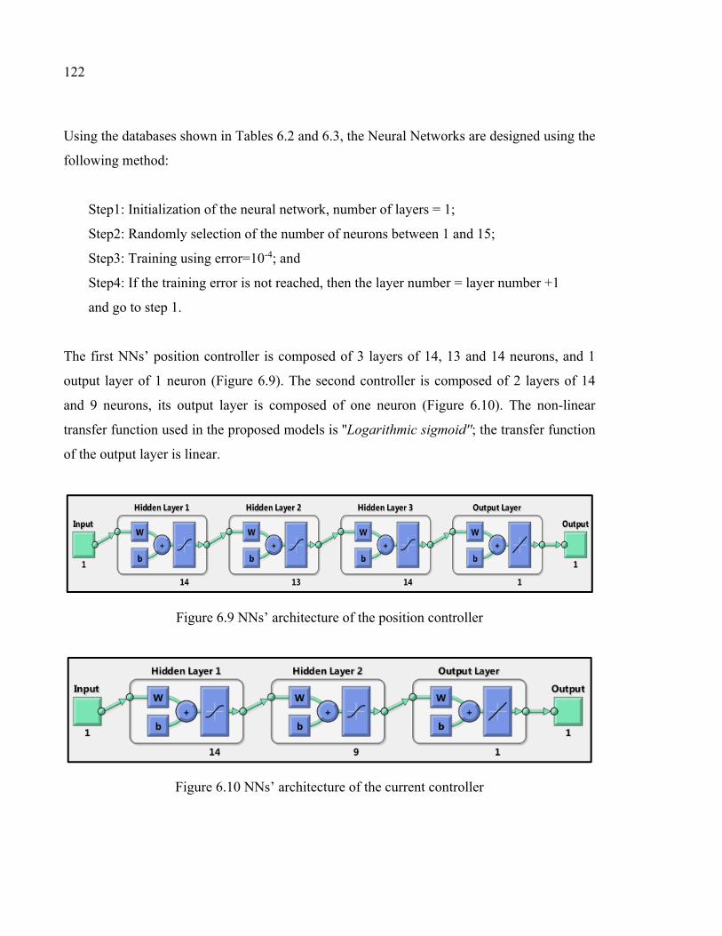
122

Using the databases shown in Tables 6.2 and 6.3, the Neural Networks are designed using the

following method:

Step1: Initialization of the neural network, number of layers = 1;

Step2: Randomly selection of the number of neurons between 1 and 15;

Step3: Training using error=10-4; and

Step4: If the training error is not reached, then the layer number = layer number +1

and go to step 1.

The first NNs’ position controller is composed of 3 layers of 14, 13 and 14 neurons, and 1

output layer of 1 neuron (Figure 6.9). The second controller is composed of 2 layers of 14

and 9 neurons, its output layer is composed of one neuron (Figure 6.10). The non-linear

transfer function used in the proposed models is ''Logarithmic sigmoid''; the transfer function

of the output layer is linear.

Figure 6.9 NNs’ architecture of the position controller

Figure 6.10 NNs’ architecture of the current controller

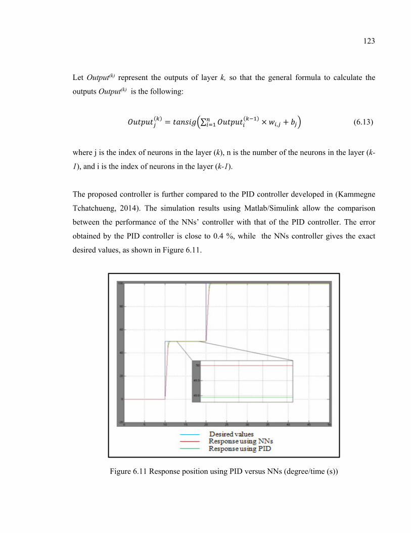
123

Let Output(k) represent the outputs of layer k, so that the general formula to calculate the

outputs Output(k) is the following:

( ) = ∑ ( ) × , + (6.13)

where j is the index of neurons in the layer (k), n is the number of the neurons in the layer (k-

1), and i is the index of neurons in the layer (k-1).

The proposed controller is further compared to the PID controller developed in (Kammegne

Tchatchueng, 2014). The simulation results using Matlab/Simulink allow the comparison

between the performance of the NNs’ controller with that of the PID controller. The error

obtained by the PID controller is close to 0.4 %, while the NNs controller gives the exact

desired values, as shown in Figure 6.11.

Figure 6.11 Response position using PID versus NNs (degree/time (s))

124

6.5 Experimental work

6.5.1 Concept of the experimental work

In order to validate the performance of the controller obtained during its simulation, a HIL

(Hardware in the Loop) process is used which implements the controller simulation via the

Labview real time environment.

Labview offers not only the possibility to communicate in real time with the different

components of our hardware loop, it also allows control algorithms and model simulations to

be imported from other modeling environments through the model interface toolkit, thus, this

Labview interface enables the interaction between Labview and third-party modeling

environments.

The validation concept, shown in Figure 6.12, is based on the idea of establishing

communication channels between the hardware components, and the Simulink controller.

The Labview program ensures that all the data required for their control operations can be

read, processed and sent to a controller. This controller will generate the correct control

signal based on the external command from the operator. The type of signals and the order of

the operations are described in the following sections.

Figure 6.12 Validation concept

125

6.5.2 Experimentation and real time validation

After finding the correct controller for the simulation, we need to prepare it for real-time

testing. The target platform in our case is Windows.

6.5.2.1 Hardware

The hardware used for testing and validation is specified in Table 6.4.

Table 6.4 List of the hardware used in the experiment

The wiring and installation are specified in Figure 6.13:

Figure 6.13 Hardware installation

Hardware Characteristics

Motor Maxon motor : RE 35 Ø35 mm, Graphite Brushes, 90 Watt

Gear box Planetary Gearhead GP 32 HP Ø32 mm, 4.0 - 8.0 Nm

Encoder Encoder MR, Type L, 512 CPT, 3 Channels, with Line Driver

Drive EPOS2 24/5, Digital positioning controller, 5 A, 11 - 24 VDC

Power supply CPX400DP- programmable dual output 2 x 420 watts

126

The ''Windows Host'' communicates using USB with the programmable power supply and

the drive Maxon, this drive is used to read and process the angle position value returned by

the encoder on the motor. The DC motor is fed directly through the power supply, as seen in

Figure 6.13.

6.5.2.2 Real-Time Model

First of all, the input and output ports of the controller are created as shown in Figure 6.14;

the controller will need the desired position (input 1), the position feedback (input 3), and the

current feedback (input 2). Regarding the configuration parameters of the Matlab/Simulink

model, the solver needs to be ''discrete'' and the ''step solver'' should to be chosen as a ''fixed

step'' with a size of five millisecond (5 msec). The system target file should be

‘NIVeristand.tlc’ in order to be used with Labview in real time.

After desired form of the controller has been given the, and the configurations parameters

have been set as mentioned above, the model can be built using Matlab’s Real-Time

Workshop.

The Labview model’s function is to ensure the interface and the data exchange between the

hardware and the controller. Using the CPX400 DP library in Labview, a USB

communication channel is established with the power supply; through this channel, we are

able to perform some actions such as opening a session, initializing a device,

enabling/disabling the output, settling the voltage value and reading the average current

value.

127

Figure 6.14 Simulink / Labview real-time model

For the calculations of position values, the Maxon drive is used to read and process the

encoder signal and return the exact angle; some operations are needed to obtain their values

in degrees.

The Labview program will need to load the controller model as a Dynamic Link Library

(DLL), which would be generated during the preparation step when building the Matlab

Simulink model. This task is performed using the Model Interface Toolkit VIs by specifying

the path of the generated DLL in order to load it, and by obtaining the sampling time.

6.5.2.3 Validation Results

A step of 50o and another of 100o were sent to the motor in order to test the performance of

the implemented controller (Figure 6.15). The results obtained are very good; the error for

50o is equal to 0%, while the error for 100o, is equal to 1%.

128

Figure 6.15 Experimental results

6.5.3 Wind tunnel test

The experimental results achieved by using the Price-Païdoussis blow down wind tunnel are

presented here. The pressure on the morphing surface of an ATR-42 wing is measured using

a pressure transducer to determine the pressure coefficient distribution (Cp). The

experimental results are compared with numerical values obtained using XFoil code.

6.5.3.1 Experimental test equipment

The Price-Païdoussis wind tunnel and the pressure transducer system are presented here. The

experiment was done using the Price-Païdoussis subsonic wind tunnel at the Research

Laboratory in Active Controls, Avionics and Aeroservoelasticity (LARCASE). The Price-

Païdoussis wind tunnel is presented in Figure 6.16. This subsonic wind tunnel is equipped

with two test chambers; the first provides a maximum airspeed of 60 m/s and the second

offers a maximum airspeed of 40 m/s.

129


The measurement system was the Multitube Manometer tubes system, as its name indicates,

this system is equipped with thirty-six tube tilting manometers to measure pressures taken

from pressure taps on the ATR-42 morphing wing model (Figure 6.17) in the Price-

Païdoussis subsonic wind tunnel. The tubes are filled with colored water to obtain very good

visibility for the readings. The Multitube Manometer tubes transducer is shown in Figure

6.18.

Figure 6.17 ATR-42 morphing wing model

130

Figure 6.18 Multitube manometer tubes transducer

6.5.3.2 Experimental results

This section presents the results obtained at the LARCASE laboratory using the Price-

Païdoussis subsonic wind tunnel. The locations of the pressure taps along the chord on the

morphing surface of the ATR-42 wing airfoil are indicated in Table 6.5.

Table 6.5 Location of pressure taps

Pressure taps

number

1 2 3 4 5 6 7 8 8 9 11 12 13 14

Position (%of the chord)

5 10 15 20 25 30 32.5 35 37.5 40 45 50 60 70

Three flight cases were considered during the wind tunnel tests. These tests were conducted

for three different angles of attack (-2o, 0o and 2o) and one Mach number equal to 0.08 (34

m/s). The experimental results are compared with results given by XFoil code. As shown in

Figures 6.19 to 6.21, the experimental pressure coefficients Cp are in a very good agreement

with the theoretical pressure coefficients results obtained using XFoil code.

131

Figure 6.19 Experimental results (multitube manometer) of pressure coefficients Cp is for the angle of attack α=0o and Mach number=0.08

Figure 6.20 Experimental results ( multitube manometer) of pressure coefficients Cp is for the angle of attack α=2o and Mach number=0.08

132

Figure 6.21 Experimental results (multitube manometer) of pressure coefficients Cp is for the angle of attack α=-2o and Mach number=0.08

6.6 Conclusion

In this paper, a NN controller was designed and tested for anATR-42 morphing wing. The

objective is to reproduce a desired specific shape of the morphing wing using electric

actuators. A robust controller is necessary to obtain a very good precision in order to achieve

the exact desired airfoil shape. The proposed NN algorithm is used for a new closed loop

controller methodology. The NN models are designed using Matlab and are further converted

into Simulink model to be used for a closed loop controller methodology. The simulation

gave very good results; the model’s responses give the desired values. The model is

compared to a PID controller. The NN controller gives a more accurate performance than the

PID controller; during experimental tests, it gave very precise results. The pressure

coefficients obtained using wind tunnel tests are compared with the pressure coefficients

given by XFoil software, and confirm the obtainment of a very good performance level.

DISCUSSION OF RESULTS

The research performed in this thesis highlights the use of Artificial Intelligence for wind

tunnel applications, and shows how the hybridization between optimization algorithms and

prediction techniques can be used to achieve specific objectives. This section presents a

summary of the results obtained in the articles presented in chapters 3 to 6.

A hybrid approach was used in the first paper (Chapter 3), “A new methodology for wind

tunnel calibration using neural networks – an Extended Great Deluge approach”. This was

utilized to calibrate the Price-Païdoussis WT by calculating the pressure distribution in the

WTT chamber. The results were compared with the Fluent results and with the WTT

specifications. The errors were on the order of 5 %.

Two hybrid methods were used in the second and third papers: SVM-EGD and NN-EGD, in

chapters 4 and 5, respectively, and applied on the ATR-42 wing for the calculation of

pressure distributions and aerodynamic coefficients. The results obtained by these methods

were compared with the XFoil and the WTT results. The theoretical mean squared error

given by the SVM-EGD methodology (Chapter 4) was less than 0.97E-5, and the

experimental mean squared error was less than 0.113E-3. The mean error between the NN-

EGD methodology (Chapter 5) and the theoretical results was less than 2% for aerodynamic

coefficient parameters, and the experimental mean squared error was less than 0.113E-3 for

pressure coefficient parameters. Two NN-EGD approaches were integrated in the control

scheme of the ATR-42 morphing wing actuators. The NN-EGD controller was compared to

the PID controller. The error given by the NN-EGD approach did not exceed 1% compared

to the PID controller values.

A new tool was developed in the first paper, for determining the pressure distribution, or the

local 3D flow characteristics, in the test chamber section of the Price-Païdoussis Subsonic

Wind Tunnel at the LARCASE laboratory during the model calibration phase. This tool was

designed based on NN and EGD hybridization, and was further used during WTTs on an

134

ATR-42 reduced-scale wing model. This ATR-42 wing had a chord of 247 mm, span of 610

mm and a maximum thickness 25 mm, or c=247 mm, b=610 mm and t=25 mm. The WTT

chamber test section is 0.6 by 0.9 meters. A CFD analysis was performed using Fluent

software to create a dataset, required for training and validating the proposed NN-EGD

methodology, which was further tested in the Price-Païdoussis wind tunnel. This dataset

modeled the test chamber volume at 81628 points, with the pressure calculated at each point

by the Fluent software.

70% of this dataset was used for training the NN-EGD methodology, 15% for the validation

and 15% for the testing phase. During the “training” phase, an NN architecture was obtained

using the EGD metaheuristic algorithm. The optimal NN configuration was composed of 4

layers with the following number of neurons: 12, 15, 10 and 1. These results show that the

NN-EGD methodology is able to calculate the pressures at the coordinate points in the WTT

chamber. The average error of the predicted pressure given by the NN-EGD methodology

was around 5% compared to the original Fluent 3D dataset. This low average error

demonstrated that the NN-EGD methodology could offer a very good calibration of the

Price-Païdoussis wind tunnel chamber in real time (before and during the WTTs) without the

use of CFD or other conventional techniques.

In the second paper, a new hybrid methodology was designed to determine the lift, drag and

pitching moment coefficients according to the flight conditions on an ATR-42 wing. An

SVM methodology was trained and optimized using an EGD algorithm. Two main phases

were realized in this paper, a theoretical phase and an experimental phase.

In the theoretical phase, a dataset was generated using XFoil code for 101 flight cases

produced by combinations of angles of attack between -5 degrees to 5 degrees for a Mach

number equal to 0.11. A total of 79 random vectors were selected to train, 11 to validate and

11 cases were selected to test the SVM-EGD methodology. The lift, drag and pitching

moment coefficient values of the 11 test cases were compared with those calculated by XFoil

code. The mean squared error (MSE) was used to measure the precision of the proposed

135

methodology. These errors were calculated for the lift, drag and pitching moment

coefficients, with values of 0.037E-4, 0.55E-6 and 0.97E-5, respectively. These error results

indicate that the SVM-EGD methodology is very good at calculating aerodynamic

coefficients.

In the experimental phase, the optimal SVM parameters obtained by the EGD algorithm and

those obtained from an XFoil dataset during the optimization phase were utilized. The Price-

Païdoussis wind tunnel was used to generate a dataset composed of a total of 100 values of

lift, drag and pitching moment coefficients. This dataset was obtained by multiple

combinations of 25 angles of attack (between -9 degrees and 15 degrees) and 4 Mach

numbers (0.058, 0.073, 0.088 and 0.117). A total of 40 flight cases were selected randomly

from the dataset to evaluate the SVM-EGD methodology’s performance. For the lift

coefficient, the mean squared error was 6.028E-3 for a Mach number of 0.117, and it was

less than 1.4E-3 for Mach numbers equal of 0.058, 0.073 and 0.088. The mean squared error

for the numerically-predicted versus the experimental drag coefficients did not exceed

0.065E-3 for all Mach numbers. The mean squared error calculated for the pitching moment

coefficients had a maximum value of 0.113E-3. The low values of the mean squared error

indicates the robustness and precision of the SVM-EGD methodology for the calculation of

aerodynamic coefficients for different flight cases.

The third paper (Chapter 5) developed an approach based on the hybridization of NN and

EGD algorithms to determine the pressure coefficient distribution and the lift, drag and

pitching moment coefficients for an ATR-42 wing. The methodology was designed based on

a numerical dataset generated using XFoil code. It was validated theoretically, and then

experimentally using the Price-Païdoussis wind tunnel. Two NN-EGD systems were

designed, one to calculate the lift, drag and pitching moment coefficients; and another to

calculate the pressure distribution.

136

Several numerical and experimental tests were performed to validate these two NN-EGD

systems. The first system was trained using the numerical dataset generated at Mach number

0.1 and at a range of angles of attack (from -5 degrees to 5 degrees). From the 101 cases

generated by this dataset, approximately 20% were used for the validation and testing phases,

corresponding to 11 random vectors for each phase. The second NN-EGD system was trained

using a numerical dataset composed of 11 combinations of angles of attack varying between -

5 degrees and 5 degrees with Mach number 0.1. This approach was further tested with 2

randomly selected angles of attack (-2 degrees and 3 degrees).

In the numerical analysis, the first NN-EGD system was trained using theoretical XFoil data

to calculate aerodynamic coefficients. Optimized by the EGD algorithm, the NN architecture

was composed by 12, 8, 9 and 3 neurons distributed on 4 layers. The second NN-EGD

system was designed with the goal of calculating the pressure distribution. The optimal NN

architecture was again composed of 4 layers, 3 of which had 10 neurons and the fourth, the

output layer, containing only one. The results obtained using the first NN-EGD system were

compared with XFoil results, and proved to be well-approximated, with the lift, drag forces,

and the pitching moment coefficients having differences of less than 0.6%, 1.2% and 2%,

respectively. The pressure distribution calculated using the second NN-EGD system was

compared with that given by XFoil code. The results for the two tested cases show a very

good prediction quality, while the average percentage error of the pressure distribution did

not exceed 5%.

The tests for the experimental analysis were carried out in the Price-Païdoussis Subsonic

wind tunnel. Due to equipment limitations, only the pressure distribution on an ATR-42 wing

was measured with 3 different systems. Thirteen wind tunnel cases were considered for

angles of attack between -2 degrees and 2 degrees, and 3 Mach numbers (0.08, 0.09 and 0.1).

The low mean squared error, which did not exceed 3E-3 for all test cases, clearly indicates

the validity of the proposed NN-EGD approach’s pressure distribution calculations for an

ATR-42 wing.

137

The fourth paper (Chapter 6) presents a controller designed to generate a desired shape of the

ATR-42 morphing wing, utilizing two NN approach. . One of these is position controller that

manages the appropriate current according to the actuator positions’ errors, and the other is a

current controller designed to manage the necessary voltage according to the error of the

current needed by the electrical motors to achieve the desired actuator positions.

The NN methodology was implemented in two steps. In the first step, two datasets were

generated by a "trial and error" process. These datasets were then used for the training phase.

The NNs controllers were integrated in the control loop of the electrical actuation systems of

the ATR-42 morphing wing in the second step.

The simulation was performed using Matalb/Simulink, in which the proposed controller

model was simulated with a PID controller to validate its ability to provide the required wing

shape deformations. The numerical results show that the NN controller was able to perform

exact shape deformations. However, the PID controller gave shape deformations with an

error close to 0.4%. The experimental analysis was performed using tools and equipment

available at the LARCASE. The proposed controller gave a very good precision in providing

the desired shape deformations, as the error for these deformations did not exceed 1%.

CONCLUSION AND RECOMMENDATIONS

This thesis presents new methodologies and has shown how they can be used in numerous

wind tunnel applications. Several conclusions can be made on the use of hybrid artificial

intelligence methods and their combination with Extended Great Deluge methods,

particularly regarding their performance in solving different problems including wind tunnel

calibration, calculation of aerodynamic coefficients, and the control of a morphing wing

shape.

A wind tunnel calibration methodology was implemented as a means to control the pressure

distribution inside a wind tunnel test section. Based on CFD analysis of a 3D airfoil wing, a

unique approach using a hybridization of NN and EGD algorithms was designed. This

approach makes it possible to control and assure the good functioning of the Price-Païdoussis

subsonic blow down wind tunnel by estimating the 3D flow inside the test chamber. This

hybrid method is easier to use than CFD methods or other experimental techniques, as, the

pressure can be calculated more rapidly. The validation was performed by using

experimental tests carried out in the Price-Païdoussis subsonic blow down wind tunnel and

by using CFD simulations, and demonstrated the accuracy of the NN-EGD hybrid approach.

Two new hybrid methodologies were proposed for aerodynamic analysis applications. These

two AI approaches allow to predict the lift forces, drag forces, pitching moments, and the

pressure distributions on both wing models of an ATR-42 aircraft. They both provided the

required aerodynamic coefficients almost instantaneously and with high accuracy for the

flight cases considered. The validation of these approaches shows that optimizing the NNs

and the SVM parameters offers the best compromise between the quality of results and the

computing time. Validations performed using numerical and experimental analyses for

several flight cases revealed the reliability of these two methodologies in addition to their

low errors and rapid computing time. Thanks to these advantages, the proposed

methodologies are very well suited to predict and thus to estimate the aerodynamic

coefficients and the pressure distribution on ATR-42 wing models, as well as being ideal for

140

control loop integration on a morphing wing during WTTs. These methodologies have also

been proven effective for WT calibration.

As discussed in this thesis, the highly accurate optimization and the learning capacity of

artificial intelligence methods are key to obtaining a good regression and thereby achieving

excellent results. The Extended Great Deluge methodology was adapted to optimize the

proposed NN and the SVM methodologies. This algorithm was selected because it can easily

be adapted to the problems under evaluation. Its limited number of parameters (only two), its

very good performance at solving several optimization problems in different fields and its

novelty in aeronautical applications all contributed to its selection. Even when the nature of

the problems are NP-hard, the EGD can perform a very good optimization of the NN and of

the SVM approaches in a very reasonable computing time combined with very good results.

The morphing wing structure consists of a flexible part that changes its shape by means of

actuation systems to obtain the desired airfoil shapes. The main aim is to improve the

aerodynamic performance of this technology. Controllers were designed and integrated in the

control loop of an ATR-42 morphing wing electrical actuator system. The proposed

controller was shown to be capable of successfully managing the current and the voltage

needed by the actuators to provide the desired deformations of the flexible skin; deformations

designed to generate the optimal airfoils to reduce drag forces.

The research presented here could be further be improved by work incorporating the

following recommendations:

For a large operating range of the calibration methodology, the parameters of the

wing model (the airfoil, sweep, cord, span, etc.) needs to be considered in 3D

analysis. This will require additional high fidelity CFD analysis to generate a larger

dataset. Training the calibration method using a larger dataset will make it possible to

apply it to wider range of wing models.

141

To cover the whole flight trajectory, the take-off and the landing phases could be

added to these studies. Aerodynamic analyses of take-off and landing phases should

be performed to generate the datasets required to train the prediction approaches.

Applying the proposed methodologies to additional flight conditions would improve

their performance and utility, and other flight parameters could be added, such as the

angle of sideslip, the flaps and the slats deflection, the ailerons deflection, etc.

Instead of the trial and error technique used here, an optimization algorithm could

automatically determine the optimal dataset and thereby improve the control system.

The use of another metaheuristic algorithm to optimize the proposed approaches is

recommended to compare results and to justify the use of the Extended Great Deluge

algorithm.

LIST OF REFERENCES

ASHRAE Standard 41.7-78. 1978. Procedure for fluid flow measurement of gases. American Society of Heating, Refrigerating and Air-Conditioning Engineers, Inc.

ASHRAE Standard 41.2. 1987. Standard methods for laboratory airflow measurement

American Society of Heating, Refrigerating and Air-Conditioning Engineers, Inc. Abha, Lunia, M Issac Kakkattukuzhy, K Chandrashekhara et E Watkins steve. 2000. «

Aerodynamic testing of a smart composite wing using fiber-optic strain sensing and neural networks ». Smart Materials and Structures, vol. 9, no 6, p. 767-773.

Arnaud, Rémi, et Fabrice Poirion. 2014. « Stochastic annealing optimization of uncertain

aeroelastic system ». Aerospace science and technology, vol. 39, p. 456-464. Asadi, F., M. Di Penta, G. Antoniol et Y. G. Gueheneuc. 2010. « A Heuristic-Based

Approach to Identify Concepts in Execution Traces ». In Software Maintenance and Reengineering (CSMR), 2010 14th European Conference on. (15-18 March 2010), p. 31-40.

Ateme-Nguema, Barthélemy H. 2007. « Conception optimale des cellules de fabrication

flexibles basée sur l'approche par réseaux de neurones ». Montréal, École de technologie supérieure.

Barlow, Jewel B., William H. Rae et Alan Pope. 1999. Low-speed wind tunnel testing (1999),

3rd ed. Baron A, Benedict B, Branchaw N, Ostry B, Pearsall J, Perlman G et Selstrom J. 2003.

Morphing wing (MoW). Coll. « ASEN 4018 Senior Projects ». Boulder, Colorado, USA.

Ben Mosbah, Abdallah, Ruxandra M. Botez et Thien My Dao. 2013. « New methodology for

calculating flight parameters with neural network – EGD method ». In AÉRO 13, 60th Aeronautics Conference and AGM. (Toronto - Canada, 30 April - 2 May, 2013).

Ben Mosbah, Abdallah, Ruxandra M. Botez et Thien My Dao. 2013. « New methodology for

calculating flight parameters with neural network - Extended Great Deluge method applied on a reduced scale wind tunnel model of an ATR-42 wing ». In AIAA Modeling and Simulation Technologies (MST) Conference. Coll. « Guidance, Navigation, and Control and Co-located Conferences »: American Institute of Aeronautics and Astronautics.

144

Ben Mosbah, Abdallah, Ruxandra M. Botez et Thien My Dao. 2014. « New Methodology for the Calculation of Aerodynamic Coefficients on ATR-42 Scaled Model With Neural Network – EGD Method ». In ASME 2014 International Mechanical Engineering Congress and Exposition. (Montreal, Quebec, Canada, November 14–20, 2014). ASME.

Ben Mosbah, Abdallah, Ruxandra M. Botez et Thien My Dao. 2014. « New methodology

for the prediction of the aerodynamic coefficients of an ATR-42 scaled wing model ». In SAE 2014 aerospace systems and technology conference. (Cincinnati, OH, USA, 2014 September 23–25).

Ben Mosbah, Abdallah. 2011. « Optimisation de l'ordonnancement cellulaire avec

métaheuristiques ». Montréal, École de technologie supérieure. Ben Mosbah, Abdallah, et Thien-My Dao. 2010. « Optimimization of group scheduling using

simulation with the meta-heuristic Extended Great Deluge (EGD) approach ». In Industrial Engineering and Engineering Management (IEEM), 2010 IEEE International Conference. (7-10 Dec. 2010), p. 275-280.

Ben Mosbah, Abdallah, et Thiên-My Dao. 2013. « Optimisation of manufacturing cell

formation with extended great deluge meta-heuristic approach ». International Journal of Services Operations and Informatics, vol. 7, no 4, p. 280-293.

Ben Mosbah, Abdallah, et Thien My Dao. 2010. « Optimimization of Group Scheduling

Using Simulation with the Meta-Heuristic Extended Great Deluge (EGD) Approach ». In Industrial Engineering and Engineering Management (IEEM), IEEE International conference. (Macao, China, december, 07-10, 2010), p. 275-280.

Ben Mosbah, Abdallah, Manuel Flores Salinas, Ruxandra Botez et Thien-My Dao. 2013. «

New Methodology for Wind Tunnel Calibration Using Neural Networks - EGD Approach ». SAE International Journal of Aerospace, vol. 6, no 2, p. 761-766.

Ben Mosbah, Abdallah et Dao, Thien-My. 2011. « Optimization of group scheduling

problem using the hybride meta-heuristic extended great deluge approach : a case study ». Journal of management and egineering integration, vol. 4, no 2, p. 1-13.

Ben Mosbah, Abdallah et Dao, Thien My. 2011. « Optimization of Manufacturing Cell

Formation with Extended Great Deluge Metaheuristic Approach ». In International Conference on. Industrial Engineering and Systems Management. (May, 25-27, 2011).

Bigdeli, Nooshin, Karim Afshar, Amin Shokri Gazafroudi et Mostafa Yousefi Ramandi.

2013. « A comparative study of optimal hybrid methods for wind power prediction in wind farm of Alberta, Canada ». Renewable and Sustainable Energy Reviews, vol. 27, p. 20-29.

145

Boëly, N., et R. M. Botez. 2010. « New Approach for the Identification and Validation of a Nonlinear F/A-18 Model by Use of Neural Networks ». IEEE Transactions on Neural Networks, vol. 21, no 11, p. 1759-1765.

Boëly, N., R. M. Botez et G. Kouba. 2011. « Identification of a non-linear F/A-18 model by

the use of fuzzy logic and neural network methods ». Proceedings of the Institution of Mechanical Engineers, Part G: Journal of Aerospace Engineering, vol. 225, no 5, p. 559-574.

Boria, Frank, Bret Stanford, Scott Bowman et Peter Ifju. 2009. « Evolutionary Optimization

of a Morphing Wing with Wind-Tunnel Hardware in the Loop ». AIAA Journal, vol. 47, no 2, p. 399-409.

Brossard, Jérémy. 2013. Commande en boucle fermée sur un profil d'aile déformable dans la

soufflerie Price-Païdoussis (2013). Montréal: École de technologie supérieure, 1 ressource en ligne (xxvi, 185 pages) p.

Burke, Edmund, Yuri Bykov, James Newall et Sanja Petrovic. 2004. « A time-predefined

local search approach to exam timetabling problems ». IIE Transactions, vol. 36, no 6, p. 509-528.

Campanile, L. F., et D. Sachau. 2000. « The Belt-Rib Concept: A Structronic Approach to

Variable Camber ». Journal of Intelligent Material Systems and Structures, vol. 11, no 3, p. 215-224.

Chandrasekhara, M. S., L. W. Carr, M. C. Wilder, G. N. Paulson et C. D. Sticht. 1997. «

Design and development of a dynamically deforming leading edge airfoil for unsteady flow control ». In Instrumentation in Aerospace Simulation Facilities, 1997. ICIASF '97 Record., International Congress on. (29 Sep-2 Oct 1997), p. 132-140.

Chen, Daqing, et Phillip Burrell. 2002. « On the optimal structure design of multilayer

feedforward neural networks for pattern recognition ». International Journal of Pattern Recognition and Artificial Intelligence, vol. 16, no 04, p. 375-398.

Cherkassky, Vladimir, et Yunqian Ma. 2004. « Practical selection of SVM parameters and noise estimation for SVM regression ». Neural Networks, vol. 17, no 1, p. 113-126.

Cornuejols, Antoine, Laurent Miclet et Yves Kodratoff. 2002. Apprentissage artificiel :

concepts et algorithmes (2002). Paris: Éditions Eyrolles. Culham, Ralph G. 2001. Fans Reference Guide (2001), 4. Toronto, Canada. Daniel, Coutu. 2010. « Conception et exploitation d'une structure active pour une aile

laminaire adaptative expérimentale ». Montréal, École de technologie supérieure.

146

Daniel, Coutu, Brailovski Vladimir et Terriault Patrick. 2010. « Optimization Design of an Active Extrados Structure for an Experimental morphing Laminar wing ». Aerospace Science and Technology, vol. 14, no 7, p. 451–458.

David, Munday, et Jacob Jamey. 2001. « Active control of separation on a wing with

conformal camber ». In 39th Aerospace Sciences Meeting and Exhibit. Coll. « Aerospace Sciences Meetings »: American Institute of Aeronautics and Astronautics. (Reno, NV, U.S.A).

De Jesus-Mota, Sandrine , et Ruxandra Botez. 2009. « New Identification Method Based on

Neural Network for Helicopters from Flight Test Data ». In AIAA Atmospheric Flight Mechanics Conference. Coll. « Guidance, Navigation, and Control and Co-located Conferences »: American Institute of Aeronautics and Astronautics. (Chicago, Illinois).

Drela, Mark, et Michael B. Giles. 1987. « Viscous-inviscid analysis of transonic and low

Reynolds number airfoils ». AIAA Journal, vol. 25, no 10, p. 1347-1355. Dueck, Gunter. 1993. « New Optimization Heuristics: The Great Deluge Algorithm and the

Record-to-Record Travel ». Journal of Computational Physics, vol. 104, no 1, p. 86-92.

El Asli, Neila. 2008. « Approche hybride basée sur les machines à vecteurs de support et les

algorithmes génétiques pour l'estimation des coûts de fabrication ». Montréal, École de technologie supérieure.

Faller, William E., et Scott J. Schreck. 1996. « Neural networks: Applications and

opportunities in aeronautics ». Progress in Aerospace Sciences, vol. 32, no 5, p. 433-456.

Fiannaca, Antonino, Giuseppe Di Fatta, Riccardo Rizzo, Alfonso Urso et Salvatore Gaglio.

2013. « Simulated annealing technique for fast learning of SOM networks ». Neural Computing and Applications, vol. 22, no 5, p. 889-899.

Florian, R Menter. 2009. « Review of the shear-stress transport turbulence model experience

from an industrial perspective ». International Journal of Computational Fluid Dynamics, vol. 23, no 4, p. 305-316.

Florian, M R, R B Langtry, S R Likki, Y B Suzen, P G Huang et S Völker. 2004. « A

correlation-based transition model using local variables—Part I: model formulation ». Journal of Turbomachinery vol. 128, no 3, p. 413-422.

Grigorie, Teodor Lucian , et Ruxandra Mihaela Botez. 2011. « New Applications of Fuzzy

Logic Methodologies in Aerospace Field ». In Fuzzy Controllers, Theory and Applications. p. 253-296. USA: InTech.

147

Grigorie, Lucian, Ruxandra Botez, Andrei Popov, Mahmood Mamou et Youssef Mebarki. 2011. « An Intelligent Controller based Fuzzy Logic Techniques for a Morphing Wing Actuation System using Shape Memory Alloy ». In 52nd AIAA/ASME/ASCE/AHS/ASC Structures, Structural Dynamics and Materials Conference. Coll. « Structures, Structural Dynamics, and Materials and Co-located Conferences »: American Institute of Aeronautics and Astronautics. (Denver, Colorado, U.S.A).

Grigorie, TL, R Botez, AV Popov, M Mamou et YA Me´barki. 2012. « A hybrid fuzzy logic

proportional integral-derivative and conventional on-off controller for morphing wing actuation using shape memory alloy Part 2: Controller implementation and validation ». The Aeronautical Journal vol. 116, p. 451-465.

Grigorie, TL, R Botez, AV Popov, M Mamou et YA Me´barki. 2012. « A hybrid fuzzy logic

proportional-integral-derivative and conventional on-off controller for morphing wing actuation using shape memory alloy Part 1: Morphing system mechanisms and controller architecture design ». The Aeronautical Journal, vol. 116, p. 433-449.

Grigorie, T L, et R M Botez. 2009. « Adaptive neuro-fuzzy inference system-based

controllers for smart material actuator modelling ». Proceedings of the Institution of Mechanical Engineers, Part G: Journal of Aerospace Engineering, vol. 223, no 6, p. 655-668.

Grigorie, T. L., R. M. Botez et A. V. Popov. 2009. « Adaptive neuro-fuzzy controllers for an

open-loop morphing wing system ». Proceedings of the Institution of Mechanical Engineers, Part G: Journal of Aerospace Engineering, vol. 223, no 7, p. 965-975.

Grigorie, Teodor Lucian , Ruxandra Mihaela Botez et Andrei Vladimir Popov. 2012. «

Fuzzy Logic Control of a Smart Actuation System in a Morphing Wing ». In Fuzzy Controllers- Recent Advances in Theory and Applications. InTech.

Grigorie, T. L., A.V. Popov, R.M. Botez, M. Mamou et Y. Mebarki. 2010. « A Morphing

Wing used Shape Memory Alloy Actuators New Control Technique with Bi-positional and PI Laws Optimum Combination - Part 1: Design Phase ». In 7th International Conference on Informatics in Control, Automation and Robotics, ICINCO 2010. (Funchal, Madeira, Portugal, June 15-18, 2010).

Grigorie, T L, A V Popov, R M Botez, M Mamou et Y Mébarki. 2012. « On–off and

proportional–integral controller for a morphing wing. Part 1: Actuation mechanism and control design ». Proceedings of the Institution of Mechanical Engineers, Part G: Journal of Aerospace Engineering, vol. 226, no 2, p. 131-145.

148

Grigorie, T L, Botez R, Popov AV, Mamou M et Me´barki Y. 2011. « Application of fuzzy logic in the design and control of a morphing wing using smart material actuators. ». In 58th aeronautics conference and AGM, AERO. (Montreal, Canada, April 26-28, 2011).

Grigorie, T L, A V Popov, R M Botez, M Mamou et Y Mébarki. 2012. « On–off and

proportional–integral controller for a morphing wing. Part 2: Control validation – numerical simulations and experimental tests ». Proceedings of the Institution of Mechanical Engineers, Part G: Journal of Aerospace Engineering, vol. 226, no 2, p. 146-162.

Ha, C. M. 1991. « Neural networks approach to AIAA aircraft control design challenge ». In

Navigation and Control Conference. (New Orleans,LA,U.S.A.). AIAA. Hacioglu, Abdurrahman. 2007. « Fast Evolutionary Algorithm for Airfoil Design via Neural

Network ». AIAA Journal, vol. 45, no 9, p. 2196-2203. Haiping, Fei, Zhu Rong, Zhou Zhaoying et Wang Jindong. 2007. « Aircraft flight parameter

detection based on a neural network using multiple hot-film flow speed sensors ». Smart Materials and Structures, vol. 16, no 4, p. 1239-1245.

Hebert, Rauch, Kline-Schoder Robert, Adams J. et Youssef Hussein. 1993. « Fault detection,

isolation, and reconfiguration for aircraft using neural networks ». In Guidance, Navigation and Control Conference. (Monterey,CA,U.S.A.), p. 1527-1537.

Helge, Aagaard Madsen, et Filippone Antonino. 1995. « Implementation and Test of the

XFoil Code for Airfoil Analysis and Design ». RisØ National Laboratory, Roskilde, Denmark p. 59.

Holland, J. H. 1975. «Adaptation in Neural and Artificial Systems». University of Michigan

Press. Houghton, E. L., et P. W. Carpenter. 1993. Aerodynamics for engineering students (1993),

4th ed.. Huawang, Shi, et Li Wanqing. 2010. « Evolving Artificial Neural Networks Using Simulated

Annealing-based Hybrid Genetic Algorithms ». Journal of Software, vol. 5, no 4, p. 353-360.

Huiyuan, Fan, Dulikravich George et Han Zhenxue. 2004. « Aerodynamic Data Modeling

Using Support Vector Machines ». In 42nd AIAA Aerospace Sciences Meeting and Exhibit. Coll. « Aerospace Sciences Meetings »: American Institute of Aeronautics and Astronautics. (Reno, Nevada, U.S.A)

149

Hunt, K. J., D. Sbarbaro, R. Żbikowski et P. J. Gawthrop. 1992. « Neural networks for control systems—A survey ». Automatica, vol. 28, no 6, p. 1083-1112.

Ignatyev, Dmitry I., et Alexander N. Khrabrov. 2015. « Neural network modeling of

unsteady aerodynamic characteristics at high angles of attack ». Aerospace Science and Technology, vol. 41, p. 106-115.

ISO 3966. 2008. Calculation of local velocities from measured differential pressures using

The Log-Tchebycheff method. Ilkay, Yavrucuk, Prasad, J.V.R., et Calise J. Anthony. 2001. « Adaptive limit detection and

avoidance for carefree maneuvering ». In AIAA Atmospheric Flight Mechanics Conference and Exhibit. (Montreal, QC, Canada., August 6–9, 2001), p. 4003.

Iyer, Srikanth K., et Barkha Saxena. 2004. « Improved genetic algorithm for the permutation

flowshop scheduling problem ». Computers and Operations Research, vol. 31, no 4, p. 593-606.

Jang, Jyh-Shing R. 1991. « Fuzzy Modeling Using Generalized Neural Networks Kalman

Filter Algorithm ». In AAAI-91. (Anaheim Convention Center, Anaheim, California, July 14-19, 1991), p. 762-767.

Jin-peng, Liu, Dong-xiao Niu, Hong-yun Zhang et Guan-qing Wang. 2013. « Forecasting of

wind velocity: An improved SVM algorithm combined with simulated annealing ». Journal of Central South University, vol. 20, no 2, p. 451-456.

Joel, Hetrick, Osborn Russell, Kota Sridhar, Flick Peter et Paul Donald. 2007. « Flight

Testing of Mission Adaptive Compliant Wing ». In 48th AIAA/ASME/ASCE/AHS/ASC Structures, Structural Dynamics, and Materials Conference. Coll. « Structures, Structural Dynamics, and Materials and Co-located Conferences »: American Institute of Aeronautics and Astronautics. (Honolulu, Hawai, U.S.A).

Johnson, Matthew D., et Kamran Rokhsaz. 2000. « Using Artificial Neural Networks and

self-organizing maps for detection of airframe icing ». In Atmospheric Flight Mechanics Conference. Coll. « Guidance, Navigation, and Control and Co-located Conferences »: American Institute of Aeronautics and Astronautics. (Denver, CO, U.S.A).

Johnson, Matthew D., et Kamran Rokhsaz. 2001. « Using Artificial Neural Networks and

Self-Organizing Maps for Detection of Airframe Icing ». Journal of Aircraft, vol. 38, no 2, p. 224-230.

150

Kammegne Tchatchueng, M. J., L. T. Grigorie, R. M. Botez et A. Koreanschi. 2014. « Design and validation of a position controller in the Price-Païdoussis wind tunnel ». In IASTED Modeling, Simulation and Control conference. (Innsbruck, Austria, 17-19 February, 2014).

Kearns, M., et L. G. Valiant. 1989. « Crytographic limitations on learning Boolean formulae

and finite automata ». In Proceedings of the twenty-first annual ACM symposium on Theory of computing. (Seattle, Washington, USA), p. 433-444.

Keerthi, S. S. . 2002. « Efficient tuning of SVM hyperparameters using radius/margin bound

and iterative algorithms ». IEEE Transactions on Neural Networks, vol. 13, no 5, p. 1225-1229.

Kirkpatrick, S., C. D. Gelatt et M. P. Vecchi. 1983. « Optimization by Simulated Annealing

». Science, vol. 220, no 4598, p. 671-680. Kouba, Gabriel, Ruxandra Botez et Nicholas Boely. 2009. « Identification of F/A-18 model

from flight tests using the fuzzy logic method ». In 47th AIAA Aerospace Sciences Meeting including The New Horizons Forum and Aerospace Exposition. Coll. « Aerospace Sciences Meetings »: American Institute of Aeronautics and Astronautics. (Orlando, Florida, US), p. 5-8.

Kouba, Gabriel, Ruxandra Mihaela Botez et Nicolas Boely. 2010. « Fuzzy Logic Method

Use in F/A-18 Aircraft Model Identification ». Journal of Aircraft, vol. 47, no 1, p. 10-17.

Kumpati, S Narenda, et M A L Thathachar. 1974. « Learning Automata - A Survey ». IEEE

Transactions on System, Man, and Cybernetics, vol. SMC-4, no 4, p. 323-334. Lahiri, S. K., et K. C. Ghanta. 2008. « The support vector regression with the parameter

tuning assisted by a differential evolution technique: study of the critical velocity of a slurry flow in a pipeline ». Chemical Industry and Chemical Engineering Quarterly, vol. 14, no 3, p. 191-203.

Lettvin, J.Y., H.R. Maturana, W.S. McCulloch et W.H. Pitts. 1959. « What the Frog's Eye

Tells the Frog's Brain ». Proceedings of the IRE, vol. 47, no 11, p. 1940-1951. Linse, Dennis J., et Robert F. Stengel. 1993. « Identification of aerodynamic coefficients

using computational neural networks ». Journal of Guidance, Control, and Dynamics, vol. 16, no 6, p. 1018-1025.

Liu, Hui, Hong-qi Tian, Chao Chen et Yan-fei Li. 2013. « An experimental investigation of

two Wavelet-MLP hybrid frameworks for wind speed prediction using GA and PSO optimization ». International Journal of Electrical Power & Energy Systems, vol. 52, p. 161-173.

151

Lu, Xin-lai, Hu Liu, Gang-lin Wang et Zhe Wu. 2006. « Helicopter Sizing Based on Genetic Algorithm Optimized Neural Network ». Chinese Journal of Aeronautics, vol. 19, no 3, p. 212-218.

Martins, André Luiz , et Fernando Martini Catalano. 1997. « Aerodynamic optimization

study of a mission adaptive wing for transport aircraft ». In 15th Applied Aerodynamics Conference. Coll. « Fluid Dynamics and Co-located Conferences »: American Institute of Aeronautics and Astronautics. (Atlanta, GA, U.S.A)

Mehta, R. D. et Bradshaw P. 1979. « Design rules for small low speed wind tunnels ». The

Aeronautical Journal of the Royal Aeronautical Society, vol. 83, no 827, p. 443-449. Metropolis, Nicholas, Arianna W. Rosenbluth, Marshall N. Rosenbluth, Augusta H. Teller et

Edward Teller. 1953. « Equation of State Calculations by Fast Computing Machines ». The Journal of Chemical Physics, vol. 21, no 6, p. 1087-1092.

Mukesh, R., et Dr K. Lingadurai. 2011. « Aerodynamic Optimization Using Simulated

Annealing and its Variants ». International Journal of Engineering Trends and Technology, vol. 2, no 3, p. 73-77.

Nahas, Nabil, Abdelhakim Khatab, Daoud Ait-Kadi et Mustapha Nourelfath. 2008. «

Extended great deluge algorithm for the imperfect preventive maintenance optimization of multi-state systems ». Reliability Engineering & System Safety, vol. 93, no 11, p. 1658-1672.

Napolitano, Marsello R., et Michael Kincheloe. 1995. « On-line learning neural-network

controllers for autopilot systems ». Journal of Guidance, Control, and Dynamics, vol. 18, no 5, p. 1008-1015.

Nourelfath, Mustapha, et Nabil Nahas. 2003. « Quantized hopfield networks for reliability

optimization ». Reliability Engineering & System Safety, vol. 81, no 2, p. 191-196. Nourelfath, Mustapha, et Nabil Nahas. 2005. « Artificial neural networks for reliability

maximization under budget and weight constraints ». Journal of Quality in Maintenance Engineering, vol. 11, no 2, p. 139-151.

Pai, Ping-Feng, et Wei-Chiang Hong. 2005. « Support vector machines with simulated

annealing algorithms in electricity load forecasting ». Energy Conversion and Management, vol. 46, no 17, p. 2669-2688.

Panigrahi, P. K., Manish Dwivedi, Vinay Khandelwal et Mihir Sen. 2003. « Prediction of

Turbulence Statistics Behind a Square Cylinder Using Neural Networks and Fuzzy Logic ». Journal of Fluids Engineering, vol. 125, no 2, p. 385.

152

Pannagadatta, K. Shivaswamy, Chu Wei et Jansche Martin. 2007. « A support vector approach to censored targets ». In IEEE International Conference on Data Mining (ICDM-07). (Omaha, NE, USA 28-31 Oct. 2007).

Patrón, Roberto S. Félix, Yolène Berrou et Ruxandra M. Botez. 2015. « New methods of

optimization of the flight profiles for performance database-modeled aircraft ». vol. 229, no 10, p. 1853-1867.

Pehlivanoglu, Y. Volkan, et Oktay Baysal. 2010. « Vibrational genetic algorithm enhanced

with fuzzy logic and neural networks ». Aerospace Science and Technology, vol. 14, no 1, p. 56-64.

Peyada, N. K., et A. K. Ghosh. 2009. « Aircraft parameter estimation using a new filtering

technique based upon a neural network and Gauss-Newton method ». The Aeronautical Journal, vol. 113, no 1142, p. 243-252.

Piroozan, Parham 2005. « Pressure Measurement and Pattern Recognition by Using Neural

Networks ». In ASME 2005 International Mechanical Engineering Congress and Exposition. (Orlando, Florida, USA, November 5–11, 2005), p. 897-905.

Popov, Andrei V., Lucian T. Grigorie, Ruxandra M. Botez, Mahmoud Mamou et Youssef

Mébarki. 2010. « Closed-Loop Control Validation of a Morphing Wing Using Wind Tunnel Tests ». Journal of Aircraft, vol. 47, no 4, p. 1309-1317.

Popov, Andrei V., Lucian T. Grigorie, Ruxandra M. Botez, Mahmood Mamou et Youssef

Mébarki. 2010. « Real Time Morphing Wing Optimization Validation Using Wind-Tunnel Tests ». Journal of Aircraft, vol. 47, no 4, p. 1346-1355.

Popov, Andrei Vladimir, Teodor Lucian Grigorie, Ruxandra Mihaela Botez, Youssef

Mébarki et Mahmood Mamou. 2010. « Modeling and Testing of a Morphing Wing in Open-Loop Architecture ». Journal of Aircraft, vol. 47, no 3, p. 917-923.

Popov, A. V., M. Labib, J. Fays et R. M. Botez. 2008. « Closed-Loop Control Simulations on

a Morphing Wing ». Journal of Aircraft, vol. 45, no 5, p. 1794-1803. Rahmi, Aykan, Hajiyev Chingiz et Çalişkan Fikret. 2005. « Kalman filter and neural

network-based icing identification applied to A340 aircraft dynamics ». Aircraft Engineering and Aerospace Technology, vol. 77, no 1, p. 23-33.

Rajkumar, R., et P. Shahabudeen. 2009. « An improved genetic algorithm for the flowshop

scheduling problem ». International Journal of Production Research, vol. 47, no 1, p. 233-249.

Rebuffet, Pierre. 1966. Aérodynamique expérimentale. Paris: Dunod.

153

Ren, Yuan, et Guangchen Bai. 2011. « New Neural Network Response Surface Methods for Reliability Analysis ». Chinese Journal of Aeronautics, vol. 24, no 1, p. 25-31.

Roudbari, Alireza, et Fariborz Saghafi. 2014. « An evolutionary optimizing approach to

neural network architecture for improving identification and modeling of aircraft nonlinear dynamics ». Proceedings of the Institution of Mechanical Engineers, Part G: Journal of Aerospace Engineering, vol. 228, no 12, p. 2178-2191.

Roudbari, Alireza, et Fariborz Saghafi. 2014. « Intelligent modeling and identification of

aircraft nonlinear flight ». Chinese Journal of Aeronautics, vol. 27, no 4, p. 759-771. Ruiyi, Que, et Zhu Rong. 2012. « Aircraft Aerodynamic Parameter Detection Using Micro

Hot-Film Flow Sensor Array and BP Neural Network Identification ». Sensors, vol. 12, no 8, p. 10920-10929.

Sainmont, Corentin. 2009. « Optimisation d'une aile d'avion à profil adaptable : étude

numérique et expérimentale ». Masters thesis. École Polytechnique de Montréal. Sainmont, C., I. Paraschivoiu et D. Coutu. 2009. « Multidisciplinary Approach for the

Optimization of a Laminar Airfoil Equipped with a Morphing Upper Surface ». In Symposium on Morphing Vehicles, NATO VT-168. (Evora, Portugal).

Sajid, Amin, Volker Gerhart et Ervin Y. Rodin. 1997. « System identification via artificial

neural networks: applications to online aircraft parameter estimation ». SAE Trans, vol. 106, p. 1787-1808.

Samadzadegan, Farhad, Hadiseh Hasani et Toni Schenk. 2012. « Simultaneous feature

selection and SVM parameter determination in classification of hyperspectral imagery using Ant Colony Optimization ». Canadian Journal of Remote Sensing, vol. 38, no 2, p. 139-156.

Samy, Ihab, Ian Postlethwaite, Da-Wei Gu et John Green. 2010. « Neural-Network-Based

Flush Air Data Sensing System Demonstrated on a Mini Air Vehicle ». Journal of Aircraft, vol. 47, no 1, p. 18-31.

Savsani, V., V. Savsani, R. V. Rao et D. P. Vakharia. 2010. « Optimal weight design of a

gear train using particle swarm optimization and simulated annealing algorithms ». Mechanism and machine theory, vol. 45, no 3, p. 531-541.

Scott, Robert C. « Active control of wind-tunnel model aeroelastic response using neural

networks ». In SPIE 3991, Smart Structures and Materials 2000: Industrial and Commercial Applications of Smart Structures Technologies. (12 June 2000 ) Vol. 3991.

154

Scott, R. C., et L. E. Pado. 2000. « Active control of wind-tunnel model aeroelastic response using neural networks ». Journal of Guidance, Control, and Dynamics, vol. 23, no 6, p. 1100-1108.

Seera, M., C. P. Lim, D. Ishak et H. Singh. 2012. « Fault Detection and Diagnosis of

Induction Motors Using Motor Current Signature Analysis and a Hybrid FMM–CART Model ». IEEE Transactions on Neural Networks and Learning Systems, vol. 23, no 1, p. 97-108.

Sen, S. D., et J. A. Adams. 2013. « sA-ANT: A Hybrid Optimization Algorithm for

Multirobot Coalition Formation ». In Web Intelligence (WI) and Intelligent Agent Technologies (IAT), 2013 IEEE/WIC/ACM International Joint Conferences on. (17-20 Nov. 2013) Vol. 2, p. 337-344.

Shuhui Li, Michael, Cameron Fairbank, Donald C. Johnson, Eduardo Wunsch, Julio L.

Alonso et Julio L. Proao. 2014. « Artificial Neural Networks for Control of a Grid-Connected Rectifier/Inverter Under Disturbance, Dynamic and Power Converter Switching Conditions ». Neural Networks and Learning Systems, IEEE Transactions on, vol. 25, no 4, p. 738-750.

Sivanandam, S. N., S. N. Deepa et S. Sumathi. 2007. Introduction to Fuzzy Logic using

MATLAB (2007). Berlin, Heidelberg: Springer-Verlag Berlin Heidelberg. Smola, Alex, et Bernhard Schölkopf. 2004. « A tutorial on support vector regression ».

Statistics and Computing, vol. 14, no 3, p. 199-222. Sofla, A. Y. N., S. A. Meguid, K. T. Tan et W. K. Yeo. 2010. « Shape morphing of aircraft

wing: Status and challenges ». Materials and Design, vol. 31, no 3, p. 1284-1292. Strelec, Justin K., Dimitris C. Lagoudas, Mohammad A. Khan et John Yen. 2003. « Design

and Implementation of a Shape Memory Alloy Actuated Reconfigurable Airfoil ». Journal of Intelligent Material Systems and Structures, vol. 14, no 4-5, p. 257-273.

Suresh, S., S. N. Omkar, V. Mani et T. N. Guru Prakash. 2003. « Lift coefficient prediction at

high angle of attack using recurrent neural network ». Aerospace Science and Technology, vol. 7, no 8, p. 595-602.

Udo, Godwin J. 1992. « Neural networks applications in manufacturing processes ».

Computers & Industrial Engineering, vol. 23, no 1, p. 97-100. Üstün, B., W. J. Melssen, M. Oudenhuijzen et L. M. C. Buydens. 2005. « Determination of

optimal support vector regression parameters by genetic algorithms and simplex optimization ». Analytica Chimica Acta, vol. 544, no 1–2, p. 292-305.

155

Vapnik, Vladimir. 1999. « Three remarks on the support vector method of function estimation ». In Advances in kernel methods, sous la dir. de Bernhard, Sch, lkopf, J. C. Burges Christopher et J. Smola Alexander. p. 25-41. MIT Press.

Voitcu, Ovidiu , et Yau Shu Wong. 2003. « An Improved Neural Network Model for

Nonlinear Aeroelastic Analysis ». In 44th AIAA/ASME/ASCE/AHS/ASC Structures, Structural Dynamics, and Materials Conference. Coll. « Structures, Structural Dynamics, and Materials and Co-located Conferences »: American Institute of Aeronautics and Astronautics. (Norfolk, Virginia, U.S.A).

Vojislav, Kecman. 2001. Learning and Soft Computing, Support Vector Machines, Neural

Networks, and Fuzzy Logic Models. Cambridge, MA MIT Press. Wallach, Ricardo, Mattos Bento S. de et Girardi R. da. Mota 2006. « Aerodynamic

coefficient prediction of a general transport aircraft using neural network ». In 25th Congress of International Council of the Aeronautical Sciences. (Hamburg, Germany September 3-8, 2006), p. 1199–1214.

Wang, Qing, Weiqi Qian et Kaifeng He. 2015. « Unsteady aerodynamic modeling at high

angles of attack using support vector machines ». Chinese Journal of Aeronautics, vol. 28, no 3, p. 659-668.

Wang, Zhifei, et Hua Wang. 2012. « Inflatable Wing Design Parameter Optimization Using

Orthogonal Testing and Support Vector Machines ». Chinese Journal of Aeronautics, vol. 25, no 6, p. 887-895.

Weisshaar, Terrence A. 2006. « Morphing Aircraft Technology – New Shapes for Aircraft

Design ». In Multifunctional Structures / Integration of Sensors and Antennas. (Neuilly-sur-Seine, France), p. O1-1 - O1-20.

Wong, Bo K., Thomas A. Bodnovich et Yakup Selvi. 1997. « Neural network applications in

business: A review and analysis of the literature (1988–1995) ». Decision Support Systems, vol. 19, no 4, p. 301-320.

Wong, Bo K., Vincent S. Lai et Jolie Lam. 2000. « A bibliography of neural network

business applications research: 1994–1998 ». Computers and Operations Research, vol. 27, no 11, p. 1045-1076.

Xiao, B., Q. Hu et Y. Zhang. 2012. « Adaptive Sliding Mode Fault Tolerant Attitude

Tracking Control for Flexible Spacecraft Under Actuator Saturation ». IEEE Transactions on Control Systems Technology, vol. 20, no 6, p. 1605-1612.

156

Xu, Yuan-ming, Shuo Li et Xiao-min Rong. 2005. « Composite Structural Optimization by Genetic Algorithm and Neural Network Response Surface Modeling ». Chinese Journal of Aeronautics, vol. 18, no 4, p. 310-316.

Xuan, C. Z., Z. Chen, P. Wu, Y. Zhang et W. Guo. 2010. « Study of Fuzzy Neural Network

on Wind Velocity Control of Low-Speed Wind Tunnel ». In Electrical and Control Engineering (ICECE), 2010 International Conference. (25-27 June 2010), p. 2024-2027.

Yang, Seung-Man, Jae-Hung Han et In Lee. 2006. « Characteristics of smart composite wing

with SMA actuators and optical fiber sensors ». 3,4: IOS Press, p. 177-186. Yuying, Guo, Zhang Youmin et B. Jiang. 2010. « Multi-model-based flight control system

reconfiguration control in the presence of input constraints ». In Intelligent Control and Automation (WCICA), 2010 8th World Congress on. (7-9 July 2010), p. 5819-5824.

Zhang, Chaoyong, Peigen Li, Yunqing Rao et Shuxia Li. 2005. « A New Hybrid GA/SA

Algorithm for the Job Shop Scheduling Problem ». In Evolutionary Computation in Combinatorial Optimization: 5th European Conference, EvoCOP 2005. (Lausanne, Switzerland, March 30 - April 1, 2005), p. 246-259.

Zhang, Youmin. 2006. « A Fast and Numerically Robust Neural Network Training

Algorithm ». In Artificial Intelligence and Soft Computing – ICAISC 2006: 8th International Conference. (Zakopane, Poland, June 25-29, 2006).

École de technologie supÉrieure …espace.etsmtl.ca/1843/1/ben_mosbah_abdallah_thèse.pdf · i...

Documents