dynamic electro-thermo-mechanical modeling of a u-shaped

HAL Id: hal-01480062https://hal.archives-ouvertes.fr/hal-01480062

Submitted on 1 Mar 2017

HAL is a multi-disciplinary open accessarchive for the deposit and dissemination of sci-entific research documents, whether they are pub-lished or not. The documents may come fromteaching and research institutions in France orabroad, or from public or private research centers.

L’archive ouverte pluridisciplinaire HAL, estdestinée au dépôt et à la diffusion de documentsscientifiques de niveau recherche, publiés ou non,émanant des établissements d’enseignement et derecherche français ou étrangers, des laboratoirespublics ou privés.

Dynamic electro-thermo-mechanical modeling of aU-shaped electrothermal actuator

Hussein Hussein, Arèf Tahhan, Patrice Moal, Gilles Bourbon, YassineHaddab, Philippe Lutz

To cite this version:Hussein Hussein, Arèf Tahhan, Patrice Moal, Gilles Bourbon, Yassine Haddab, et al.. Dynamic electro-thermo-mechanical modeling of a U-shaped electrothermal actuator. Journal of Micromechanics andMicroengineering, IOP Publishing, 2016, 26 (2), pp.025010. 10.1088/0960-1317/26/2/025010. hal-01480062

https://hal.archives-ouvertes.fr/hal-01480062

https://hal.archives-ouvertes.fr

Dynamic electro-thermo-mechanical modeling of aU-shaped electrothermal actuator

Hussein Hussein, Aref Tahhan, Patrice Le Moal, GillesBourbon, Yassine Haddab and Philippe Lutz

Femto-st Institute, Besancon, France

E-mail: [email protected]

October 2015

Abstract. In this paper, we develop original analytical electro-thermal andthermo-mechanical models for the U-shaped electrothermal actuator. Dynamicsof the temperature distribution and displacement are obtained as a directrelationship between the system dimensions, material properties and electricalinput.The electrothermal model provides an exact solution of the hybrid PDEs thatdescribe the electrothermal behavior for each of the actuator’s three connectedarms. The solution is obtained using a new calculation method that allowsrepresenting an integrable function by an hybrid infinite sum of sine and cosinefunctions. Displacement at the actuator’s tip is then calculated using a quasi-static model based on the superposition and virtual works principles.Obtained temperature and displacement solutions are then discussed andcompared with finite element method (FEM) simulations via ANSYS andexperimental results. Comparisons showed good agreement making the proposedmodeling a reliable alternative which paves the way for improving the design andoptimizing the dimensions of U-shaped micro-actuators.

Keywords: U-shaped actuator, electrothermal, thermomechanical, modeling, MEMS

Submitted to: J. Micromech. Microeng.

Page 1 of 11 CONFIDENTIAL - AUTHOR SUBMITTED MANUSCRIPT JMM-101694.R1

123456789101112131415161718192021222324252627282930313233343536373839404142434445464748495051525354555657585960

2

1. INTRODUCTION

A U-Shaped electrothermal actuator is a series of threeconnected lineshaped beams (hot arm, cold arm andflexure), in a folded configuration as can be seen infigure 1.

The electrothermal heating of different arms withvariable sections leads to non-equivalent expansionsbetween the two sides of the folded actuator. The slightexpansion of those arms is amplified by the structureto generate a considerable displacement at the tip ofthe actuator.

Figure 1. U-shaped electrothermal micoractuator.

The U-shaped actuator can output high forceswith a wide range of displacement compared to othermicroactuators in MEMS. It has a repeatable behavior,long life time [1], small footprint, simple design, andtolerance to working conditions (dust, moisture...). Itsmonolithic single material structure makes it compliantwith standard MEMS-based fabrication processes.

This design, firstly introduced in 1992 [2], is beingwidely exploited during the last two decades especiallyin MEMS applications [3, 4, 5, 6, 7, 8] due to itsobvious advantages which pushed research towardsameliorating the design and the performance of theactuator.

Modeling the behavior of the actuator is a diversetask since it is an interaction of several domains :electricity, thermal distribution, structural expansionand elastic deformation. Usually, the modeling processis a sequence of two models: Electro-thermal andthermo-mechanical. The first one allows computing thetemperature values at each section as a result of jouleheating, the second one estimates the displacementat the actuator’s tip according to the obtainedtemperature distribution.

Numerous electrothermal [9, 10, 11, 12, 13] andthermomechanical [9, 11, 12, 13] models have beenpresented in previous works on the U-shaped actuator,yet few studies [13, 14, 15, 16, 17, 18] are found thathave addressed the dynamic response of the U-shapedactuator. Further, experiments and simulations in ourprevious work [18] showed a dynamic behavior thatis related to the thermal dynamic while the elasticresponse is quasistatic relatively. Therefore, dynamicelectrothermal model and static thermomechanicalmodel are required.

An analytical formulation of the steady state andtransient solutions of the electrothermal response ofa lineshaped beam are presented in [19]. As forthe U-shaped actuator, the steady state solution wasinvestigated in [20]. As for the transient solution, theproblem was solved numerically in [13] using Laplacetransformation.

As far as we know, no exact analytical solution ofthe transient electrothermal response of the actuatorwas found in literature. In the case of a simplebeam, solving the electrothermal equation revolvesaround the recognition of a Fourier series form of thegeneral solution after introducing boundary and initialconditions (Appendix A). This is not the case for theU-shaped actuator.

The difficulty in the case of the actuator lies inthe fact that the arms are differently heated, andtemperature evolution in each arm is described by anequation. This leads to a general solution in the formof a hybrid function with three sub-functions, each oneconcerns one arm of the actuator. In result, the hybridfunction cannot be recognized as a Fourier series, andno solution can be obtained with this method.

An exact analytical solution of the electrothermalproblem of the actuator is presented in this paperusing a novel calculation method that allows presentingan integrable function by a hybrid function, wheresub-functions consist of infinite sum of sines andcosines. Expression of the temperature final solutionis an infinite sum of periodic functions where all theparameters are determined. This analytical expressiondescribes evolution of the temperature distributioninside the actuator in response to an electrical input.

As for the thermo-mechanical model, in previousworks, several approaches were considered to estimatethe displacement at the tip using mainly the lengththermal expansion in each arm. The difference ofenthalpy approach was used in [12], Castiglianos theoryapproach as in [16] and Euler-Bernoulli equation wasderived to estimate the displacement in [21]. As in thevalidated model [20] where the virtual works methodwas used, in our proposed model we calculate thedisplacement using the same method but we havechosen not to make any of the simplifications donepreviously in order to obtain a solution of a moregeneral case with regard to the dimensions of theactuator.

The importance of the proposed models, liesnot only in the estimation of the displacement andtemperature distribution; but also to their capabilityof showing the effects of different parameters anddimensions on the response, a key tool for the designand optimization.

The models and solutions will be addressed inthe following sections, the actuator’s electrothermal

Page 2 of 11CONFIDENTIAL - AUTHOR SUBMITTED MANUSCRIPT JMM-101694.R1

123456789101112131415161718192021222324252627282930313233343536373839404142434445464748495051525354555657585960

3

new solution is presented followed by the thermo-mechanical modeling. Finally, analytical solutionsare discussed and compared to FEM modeling andexperimental results. Calculation method of theelectrothermal equation for a lineshaped structure isrecalled in Appendix A.

2. Electrothermal modeling of the actuator

2.1. Electrothermal equation

At the microscale, the heat transfer mechanisms aredifferent from the macroscale [22, 23]. Conduction isdominant on the free convection [23] while radiation isnegligible as in several previous studies [9, 10, 11]. Asfor, conduction should be treated as the only mode ofheat transfer in the absence of forced convection andradiation [23].

The models for the U-shaped actuator aregenerally one dimensional and have simplifyingassumptions. The temperature is considered to beuniform in the cross section for microactuators [5, 24].

In this paper, convection and radiation effects arethen neglected in the electrothermal modeling and aone dimensional simplification is considered makingthe device modeled unfolded. So, with regards tothe previous, the electrothermal partial differentialequation (PDE) that allows describing the temperatureT in terms of the space dimension x and time t is asfollows:

ρdCp∂T

∂t= J2ρ0 +Kp

∂2T

∂x2(1)

ρd: density in kgm3

Cp: specific heat in JK.kg

J : electrical current density in Am2

ρ0: electrical resistivity in Ω.mKp: thermal conductivity in W

K.m

The term on the left of (1) represents the densityof heat added due to thermal variation. The first termon the right represents the heat generation by Jouleeffect, the one next concerns the conduction betweensections and the anchors.

2.2. Actuator electrothermal response

In this section, we model the system using three elec-trothermal PDEs that are continuous in temperatureand heat flux density, one for each arm of the actuator.

The folded actuator (figure 1) is modeled unfoldedin order to match the one dimension 1D hypothesis.Coordinates and dimensions of the actuator are shownin figure 2.

Figure 2. Unfolded actuator

The temperature distribution T (x, t) in the caseof the actuator is a hybrid function with three sub-functions that represent the temperature in each of thethree arms.

T (x, t) =

Th(x, t) x ∈ [0; l1]Tc(x, t) x ∈ [l1; l2]Tf (x, t) x ∈ [l2; l3]

(2)

Where the indexes h, c and f refer to the hot arm, coldarm and flexure respectively.

In order to simplify the presentation of the model,the index k refers to the three different arms as follows:

eq.k ≡

eq.k≡h x ∈ [0; l1]eq.k≡c x ∈ [l1; l2]eq.k≡f x ∈ [l2; l3]

(3)

Three different equations allow defining theelectrothermal behavior of each arm taking inconsideration the thermal exchanges in all three asfollows:∂2Tk∂x2

=1

αp

∂Tk∂t− J2

kρ0Kp

(4)

The steady state temperature solution (Tss) hasthe following distribution in all three arms:Tkss(x) = −J

2kρ0

2Kpx2 + dk1x+ dk2

(5)

Where dh1, dh2, dc1, dc2, df1 and df2 are constants.

In addition to the boundary conditions at bothends of the actuator, there are also continuityconditions between adjacent arms in temperature andheat flux density. Considering the boundary andcontinuity conditions allows determining the values ofdk1 and dk2 in (5):

Th(0, t) = T∞ Tf (l3) = T∞Th(l1, t) = Tc(l1, t) Ah

∂T1

∂x (l1, t) = Ac∂Tc

∂x (l1, t)

Tc(l2, t) = Tf (l2, t) Ac∂Tc

∂x (l2, t) = Af∂Tf

∂x (l2, t)

(6)

Where Ah, Ac and Af are the arms section areas, andT∞ is the ambient temperature.

As in the lineshaped beam case (Appendix A), thetransient solution of temperature is a sum of the steadystate temperature solution and a sum of separatedvariable function as follows :Tk(x, t) = Tkss(x) +

∞∑n=1

Xkn(x)Tkn(t)

(7)


123456789101112131415161718192021222324252627282930313233343536373839404142434445464748495051525354555657585960

4

The general solutions of Tkn(t) and Xkn(x) havethe following forms (Appendix A): Tkn(t) = e−αpλ

2nt

Xkn(x) = akn sin(λnx) + bkn cos(λnx)= Ckn sin(λnx+ ϕkn)

(8)

Introducing the boundary and continuity condi-tions in (6) leads to the following conditions on Xkn:

Xhn(0) = 0 Xfn(l3) = 0

Xhn(l1) = Xcn(l1) Ah∂Xhn

∂x (l1) = Ac∂Xcn

∂x (l1)

Xcn(l2) = Xfn(l2) Ac∂Xcn

∂x (l2) = Af∂Xfn

∂x (l2)

(9)

Applying the conditions in (9) on Xkn allowsobtaining the equation of λn and defining the relationbetween ahn and the other constants. The relationsbetween ahn and the other constants are as follows:

bhn = 0bcnahn

=

(1− Ah

Ac

)sin(λnlh) cos(λnlh)

acnahn

= sin2(λnlh) +AhAc

cos2(λnlh)

bfnahn

= −afnahn

tan(λnl3)

afnahn

= cos(λnlc)

( Ah

Afcos(λnl2) cos(λnl1)

+ sin(λnl2) sin(λnl1)

)+ sin(λnlc)

(Ah

Acsin(λnl2) cos(λnl1)

−Ac

Afcos(λnl2) sin(λnl1)

)(10)

In addition, the equation of λn concluded from (9)is as follows:

AhAc cos(λnlh) cos(λnlc) sin(λnlf )+AhAf cos(λnlh) sin(λnlc) cos(λnlf )+AcAf sin(λnlh) cos(λnlc) cos(λnlf )−A2c sin(λnlh) sin(λnlc) sin(λnlf ) = 0

(11)

Unlike the case of a lineshaped beam, thetrigonometric equation (11) doesn’t allow obtaining asimple analytical form of λn. The values of λn forthe actuator must be then calculated numerically using(11).

Yet, a kind of periodicity for the values of λn isnoticed. If the total length of the arms can be writtenas a positive integer after scaling, then λKl

is the Klthsolution of λn:

λKl=Klπ

l3(12)

Kl is a least common multiple (lcm) betweenlengths of arms:

Kl = lcm

(lcm(lh, l3)

lh,lcm(lc, l3)

lc,lcm(lf , l3)

lf

)(13)

In result, the solutions of λn are periodic asfollows:

λKl+n = λKl+ λn (14)

In our case, l3 = 2lh, then the first part in (13)is equivalent to 2 and Kl is always an even number.In this case, λKl/2 = (Klπ)/(2l3) is also a solution ofλn. The first Kl solutions of λn are also symmetric asfollows:

λKl−n = λKl− λn (15)

Therefore, it is sufficient to calculate only the firstλn solutions for λn ≤ (Klπ)/(2l3). The other λn aredefined by symmetry and periodicity.

Returning to the modeling, the second representa-tion of Xkn(x) in (8) with Ckn, λn and ϕkn is adoptedin order to present the developed solution hereinafter:

Ckn =√a2kn + b2kn

ϕkn =

− tan−1(bkn

akn

)akn > 0

π − tan−1(bkn

akn

)akn < 0

(16)

The values of ϕkn can be concluded from (10) and(16). The relations of Ccn, Cfn with respect to Chnare as follows:

Chn = |ahn|

Ccn

Chn=

∣∣∣∣∣Ah

Acsin2(λnlh) + cos2(λnlh)

+(Ah

Ac− 1)

sin(λnlh) cos(λnlh)

∣∣∣∣∣Cfn

Chn=∣∣∣ afhn

cos(λnl3)

∣∣∣(17)

Among the 7 unknown constants in (8), λn isobtained from (11) and all others are defined accordingto only one constant Chn (17). This constant canbe calculated by introducing the initial distribution oftemperature: ∞∑n=1

Ckn sin(λnx+ ϕkn) = Tk0(x)− Tkss(x)

(18)

The recognition of a Fourier series allowscalculating the unknown constants in the case of alineshaped beam (Appendix A). Fourier series allowsrepresenting any integrable function by an infinite sumof sine waves. The sine waves are periodic on adetermined range while the sine and cosine constantsare continuous throughout the period.

These conditions are satisfied in the case of thelineshaped beam, while the hybrid and aperiodic na-ture of the temperature distribution along the actuatorprevents the application of the same principle for cal-culating the constants of the actuator electrothermalresponse.

A solution for the unknown constant in (18) ispresented in the following using a novel calculationmethod to present an integrable function by a sum ofhybrid sine and cosine functions. In order to calculatethe values of the constants Ch, Cc, Cf , ϕh, ϕc andϕf that correspond to λn = λ, we multiply the firstrow in (18) by ChAh sin(λx + ϕh), the second row by


123456789101112131415161718192021222324252627282930313233343536373839404142434445464748495051525354555657585960

5

CcAc sin(λx+ϕc) and the third row by CfAf sin(λx+ϕf ) and integrate the result over the length of theactuator:

l3∫0

∞∑n=1

CknCkAk sin(λnx+ ϕkn)

· sin(λx+ ϕk)

dx

=l3∫0

CkAk (Tk0(x)− Tkss(x)) sin(λx+ ϕk) dx(19)

Noting that:

l3∫0

eq.k dx =

l1∫0

eq.k≡hdx+l2∫l1

eq.k≡cdx+l3∫l2

eq.k≡fdx

(20)

The first side in (19) can be decomposed in twoparts:

l3∫0

∞∑n=1


· sin(λx+ ϕk)

dx

=l3∫0

∑λn 6=λ


· sin(λx+ ϕk)

dx

+l3∫0

C2kAk sin2(λx+ ϕk)

dx

(21)

Considering boundary and continuity conditionsallows canceling the first part of (21) for λn 6= λ:

l3∫0

∑λn 6=λ


· sin(λx+ ϕk)

dx = 0 (22)

The other part of (21) is equivalent to:

l3∫0

C2kAk sin2(λx+ ϕk)

dx =

12 (C2

hAhlh + C2cAclc + C2

fAf lf )

(23)

Introducing (21), (22) and (23), equation (19)becomes:l3∫0

CkAk (Tk0(x)− Tkss(x)) sin(λx+ ϕk) dx

= 12 (C2

hAhlh + C2cAclc + C2

fAf lf ).

(24)

Applying integration by parts two times to thefirst part in (24) and considering boundary andcontinuity conditions, the first part in (24) becomes:

l3∫0

CkAk (Tk0(x)− Tkss(x)) sin(λx+ ϕk) dx

= 1λ2

l3∫0

CkAk

d2

dx2 (Tk0(x)− Tkss(x))· sin(λx+ ϕk)

dx

(25)

Equations (24) or/and (25) allow defining thevalue of the unknown constant for a determinedinitial temperature distribution. In the caseof an initial uniform distribution of temperature,d2

dx2 (Tk0(x)− Tkss(x)) is equivalent to:d2

dx2(Tk0(x)− Tkss(x)) = − I2ρ0

KpA2k

(26)

In result, the integral in (24) is equivalent to:∫ l30CkAk (Tk0(x)− Tkss(x)) sin(λx+ ϕk) dx

= I2ρ0λ3Kp

−Ch

Ahcos(ϕh)

+ChAh cos(λl1 + ϕh)(

1A2

h− 1

A2c

)+CcAc cos(λl2 + ϕc)

(1A2

c− 1

A2f

)+Cf

Afcos(λl3 + ϕf )

(27)

where I is the electrical current.Combining (24) and (27) allows obtaining the

value of the unknown constant Ch with respect tothe actuator dimensions, material properties and thecorresponding λ, ϕk and Ck:

Ch =2I2ρ0

λ3Kp

(lh + lc

Ac

Ah(Cc

Ch)2 + lf

Af

Ah(Cf

Ch)2)

·

− 1A2

hcos(ϕh)

+ cos(λl1 + ϕh)(

1A2

h− 1

A2c

)+Ac

Ah

Cc

Chcos (λl2 + ϕc)

(1A2

c− 1

A2f

)+ 1AhAf

Cf

Chcos(λl3 + ϕf )

(28)

Consequently, the solution of the electrothermalproblem is obtained. The expression of thetemperature with respect to time t and position x inthe case of the actuator is as follows: Tk(x, t) = Tkss(x)

+∞∑n=1

Ckn sin(λnx+ ϕkn)e−αpλ2nt

(29)

The steady state temperature distribution Tkss(x)is obtained in (5). The values of λn are calculated from(11) and the corresponding constants Ckn and ϕkn areobtained in (16), (17) and (28).

The obtained expression (29) allows obtainingdirectly the evolution of the temperature distributioninside U-shaped actuators with determined dimensionsand material properties. In addition, this expressionallows identifying the influence of all dimensionsand parameters on the evolution of the temperaturedistribution inside the actuator.

3. Thermo-mechanical model

In this section, the displacement at the tip of theactuator is calculated based on the superposition andvirtual work principles. The displacement is seen asan image of the evolution of the thermal distributioninside the actuator.

Generally, in micro-structures, the natural fre-quency is higher. In addition, simulations and experi-ments showed that the natural frequency of the actua-tor is of several KHz, which implies that the structuraldynamic response is much faster then the electrother-mal dynamic response (The dynamic response is shown


123456789101112131415161718192021222324252627282930313233343536373839404142434445464748495051525354555657585960

6

later in Section 4). Thus, the mechanical inertia is con-sidered to be quasi-static.

The structure of the actuator allows amplifyingthe thermal expansion difference between the two sidesof the actuator. Thermal expansion of each arm occursdue to temperature rise with respect to the followingequation:

∆l =

l∫0

α (T (x)− T0) dx (30)

Where ∆l is the length expansion and α is the thermalexpansion coefficient.

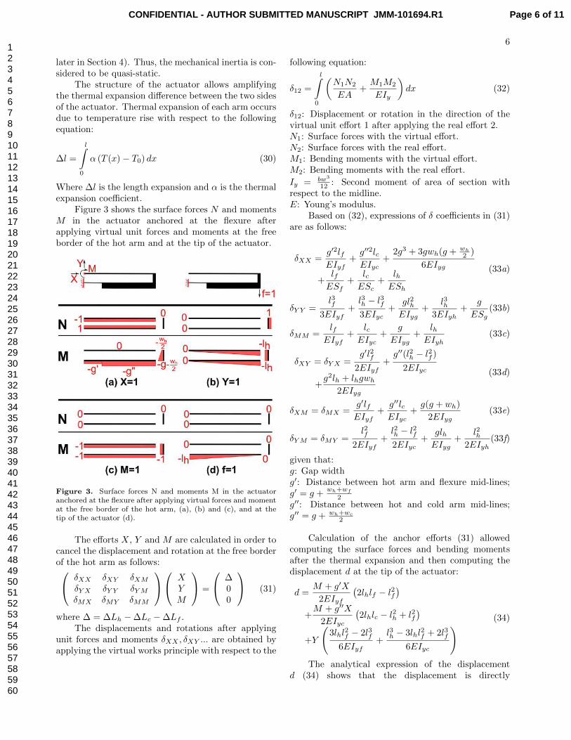
Figure 3 shows the surface forces N and momentsM in the actuator anchored at the flexure afterapplying virtual unit forces and moments at the freeborder of the hot arm and at the tip of the actuator.

Figure 3. Surface forces N and moments M in the actuatoranchored at the flexure after applying virtual forces and momentat the free border of the hot arm, (a), (b) and (c), and at thetip of the actuator (d).

The efforts X, Y and M are calculated in order tocancel the displacement and rotation at the free borderof the hot arm as follows: δXX δXY δXM

δY X δY Y δYMδMX δMY δMM

XYM

=

∆00

(31)

where ∆ = ∆Lh −∆Lc −∆Lf .The displacements and rotations after applying

unit forces and moments δXX , δXY ... are obtained byapplying the virtual works principle with respect to the

following equation:

δ12 =

l∫0

(N1N2

EA+M1M2

EIy

)dx (32)

δ12: Displacement or rotation in the direction of thevirtual unit effort 1 after applying the real effort 2.N1: Surface forces with the virtual effort.N2: Surface forces with the real effort.M1: Bending moments with the virtual effort.M2: Bending moments with the real effort.

Iy = bw3

12 : Second moment of area of section withrespect to the midline.E: Young’s modulus.

Based on (32), expressions of δ coefficients in (31)are as follows:

δXX =g′2lfEIyf

+g′′2lcEIyc

+2g3 + 3gwh(g + wh

2 )

6EIyg

+lfESf

+lcESc

+lhESh

(33a)

δY Y =l3f

3EIyf+l3h − l3f3EIyc

+gl2hEIyg

+l3h

3EIyh+

g

ESg(33b)

δMM =lf

EIyf+

lcEIyc

+g

EIyg+

lhEIyh

(33c)

δXY = δY X =g′l2f

2EIyf+g′′(l2h − l2f )

2EIyc

+g2lh + lhgwh

2EIyg

(33d)

δXM = δMX =g′lfEIyf

+g′′lcEIyc

+g(g + wh)

2EIyg(33e)

δYM = δMY =l2f

2EIyf+l2h − l2f2EIyc

+glhEIyg

+l2h

2EIyh(33f)

given that:g: Gap widthg′: Distance between hot arm and flexure mid-lines;g′ = g +

wh+wf

2g′′: Distance between hot and cold arm mid-lines;g′′ = g + wh+wc

2

Calculation of the anchor efforts (31) allowedcomputing the surface forces and bending momentsafter the thermal expansion and then computing thedisplacement d at the tip of the actuator:

d =M + g′X

2EIyf

(2lhlf − l2f

)+M + g′′X

2EIyc

(2lhlc − l2h + l2f

)+Y

(3lhl

2f − 2l3f

6EIyf+l3h − 3lhl

2f + 2l3f

6EIyc

) (34)

The analytical expression of the displacementd (34) shows that the displacement is directly


123456789101112131415161718192021222324252627282930313233343536373839404142434445464748495051525354555657585960

7

proportional to the expansion difference between twosides of the actuator.

d = k∆ (35)

4. Simulations, Experiments and discussion

The analytical models in this section are comparedwith FEM simulations and experiments and the evolu-tion of the physical aspects (such as the temperaturedistribution and displacement) is discussed.

Analytical models, FEM simulations and experi-ments are run on a doped silicon U-shaped actuatorwith the dimensions shown in figure 4. These dimen-sions are chosen to provide the required performancefor our microrobotic application [7].

Figure 4. The modeled actuator dimensions

Most of the physical properties of doped siliconare dependent of the temperature and the dopingconcentration. The thermal conductivity Kp of silicondecreases with temperature [25]. It also decreasesfor thin layers and for high impurity concentration[26]. The specific heat Cp of silicon increases withtemperature [27]. The electrical resistivity ρ0 of siliconis also thermally dependent, its evolution with dopingconcentration and temperature is clarified in [28].

A simplifying assumption considering a constantvalue for these properties is taken. This hypothesis al-lows using the analytical solution of the electrothermalmodel to simulate the temperature distribution in theactuator.

Figure 5 shows evolution of the temperaturedistribution, at several instants between 0 and 1s, afterapplying a voltage of 15V at the anchors.

The electrothermal response is calculated directlyfrom the analytical expression of T (x, t) in (29). Thephysical properties used in the calculation have thefollowing values: Ts = 298.15 K, ρd = 2330 kg/m3,Cp = 712 J/K · kg, Kp = 149 W/mK, ρ0 = 0.265Ωmm.

Different rates of temperature evolution in thethree arms of the actuator are observed in figure5. Further, figure 6 shows evolution of the averagetemperature of the hot arm, cold arm and flexureregarding the time.

Due to the lower width, the local Joule heatingis higher in the flexure at the beginning. Thus, the

Figure 5. Temperature profiles in the actuator obtainedanalytically at 0, 2, 10, 20, 40, 70, 150, 250, 500 and 1000msafter applying 15V.

Figure 6. Evolution of the average temperature with time inthe three arms of the actuator after applying 15V voltage.

initial temperature evolution is faster in the flexure,than in the hot and cold arms respectively. However,the temperature evolution rate of the flexure is limitedby the cold temperature of the anchor and the coldarm and its evolution rate starts to slow down (zoomin figure 6) consequently. From the beginning, thetemperature in the hot arm grows rapidly and despitea larger width than the flexure arm, the temperaturein the hot arm becomes quickly higher. After around100 ms, the temperature in the hot arm is closer tothe steady state and its evolution rate becomes highlyreduced whereas the temperatures in the cold and theflexure arms continue to rise until their steady state.

In result, the evolution rate of the temperaturein the hot arm is higher than the cold side (cold andflexure arms) at the beginning while it is slower whilegetting closer to the steady state. This difference inthe evolution rate is the reason behind the overshootbehavior of the actuator displacement shown later inthis paper (figure 10), where the thermal expansionin each side is related to the temperature distribution(30) and the displacement is an image of the expansiondifference (35).

A 3D FEM modeling is made using ANSYS andallows simulating the thermal distribution and the


123456789101112131415161718192021222324252627282930313233343536373839404142434445464748495051525354555657585960

8

structural deformation of the actuator after applyingelectrical voltage. The element used in the simulationSOLID226 is selected to allow a thermal-electric-structural analysis. The actuator in the simulationhas the same dimensions as in figure 4. Convection andradiation are neglected and the physical properties andboundary conditions are the same as in the analyticalmodeling.

The evolution of the average temperature in thehot arm is considered as a comparison parameter ofthe electrothermal response between the analyticalsolution and FEM simulation. The comparison isshown in figure 7 for two applied voltages (15 and 18V).

Figure 7. Comparison between the analytical model andANSYS for the evolution of the average temperature in the hotarm.

Figure 7 shows a very good agreement betweenthe presented electrothermal solution and FEMsimulations. The temperature distribution in the 3DFEM simulation is remarked to be homogeneous inthe cross section along each arm while it is slightlynon-homogeneous at the borders. This validates theone-dimensional simplifying assumption used in theelectrothermal analytical model.

Experiments that are run on microfabricatedactuators allowed us to record the displacement ofthe actuator with a high speed camera after applyingelectrical voltages.

The actuators are fabricated using single-crystalline silicon-on-insulator (SOI) wafer, with a100µm device layer, a 2µm buried oxide (SiO2) anda 380µm handle layer. The device layer with a <1-0-0> orientation is highly doped p-type and has a rangeof resistivity of 0.1− 0.3 Ωmm.

The shape of the actuator after fabrication isshown in figure 8. The active parts of the actuatorare realized in the device layer while the handlelayer serves as a support of the whole device. Theintermediate SiO2 layer is an electrical insulator, itallows separating the anchor pads electrically.

In the experiments, the actuators on wafer areplaced in a micromanipulation station under a highspeed camera. This camera allows recording thedisplacement of the actuator throughout a microscope

Figure 8. Layers of the microfabricated actuator.

with a frame rate of up to several ten thousands offrames per second. The electrical connection with theactuator is provided with 2 conductive probes that areconnected to the actuator pads. The displacement ofthe actuator after applying a step voltage is recordedon videos. Figure 9 shows two frames of an experiencevideo in the on and off state respectively. Thedisplacement is then measured directly on the videosusing a specific software. For example, the measureddisplacement in figure 9.b is around 150µm.

Figure 9. Frames from an experience video on the actuator, atthe rest position (a) and during displacement (b).

Figure 10 shows the displacement curves of theactuator with respect to time obtained from theanalytical models, FEM simulations and experiments.Displacement curves are shown for two applied voltages(15V and 18V).

Figure 10. Comparison between the analytical model, ANSYSand experiments for the displacement curves at the tip of theactuator.

Noting that the expansion coefficient α is consid-ered to be thermally dependent in the analytical calcu-lation (30) and FEM simulations. This consideration


123456789101112131415161718192021222324252627282930313233343536373839404142434445464748495051525354555657585960

9

was taken into account because of the large variationof the expansion coefficient of silicon with tempera-ture (from 2.568µm/mK at 300K to 4.258µm/mK at1000K). Yokada et al. in [29] have defined an equationfor the thermal expansion coefficient of silicon with re-spect to temperature:

α = 10−6

(3.725

(1− e−5.88·10−3(T−124)

)+5.548 · 10−4T

)(36)

Figure 10 shows an important overshoot ofdisplacement of the actuator before reaching a steadystate position. The transient shape of displacementis due to the variation of the evolution rate oftemperature distribution on the two sides of theactuator as shown in figures 5 and 6.

Fig 10 shows that this behavior of displacement iscommon between the analytical models, FEM simula-tions and experiments but with slight differences.

The displacement curves of the analytical modelsand the FEM simulation have the same shapes butwith a small shift between the two theoretical curves.Consequently, as there’s a good agreement in termsof the electrothermal response as shown in figure 7and as the displacement is equivalent to the expansiondifference (35) which is an image of the temperaturedistribution, then the difference in the calculateddisplacement returns mostly to the thermo-mechanicalmodel. This difference may return to the negligence ofthe shear force and the one dimensional simplificationin the analytical calculation. The different armsin the actuator are considered as lines and there isan uncertainty in the calculation particularly at theconnection between arms. In addition, the slightestdifference in the electrothermal model is amplified inthe displacement calculation due to the amplifyingeffect of the structure.

In the other side, there is a difference in the shapeof the displacement curves between the calculatedand experimental results as shown in figure 10.Experiments show a lower overshoot and a highersteady state final position. This difference mayexist due to the assumptions taken in the calculation(negligence of convection and radiation, boundaryconditions etc.), the uncertainty in the physicalproperties and the thermal dependence of the physicalproperties of silicon especially in the steady state wherethe actuator is overheated.

In result, the analytical models presented inthis paper show good agreement with the resultsof the FEM simulations and experiments. Analmost perfect agreement is noted in terms ofthe transient electrothermal response between theanalytical solution and FEM simulations despite the1D simplification of the analytical model.

Less agreement is noted in the calculateddisplacement. A small shift between the displacement

curves is noted with the FEM simulation results and aslight difference in the shape of these curves is notedwith the experimental results.

Originality of the electrothermal analytical modelis that it provides an exact solution of the hybrid PDEsthat describe the electrothermal behavior of the threearms of the actuator. The calculation method can beextended to any number of connected hybrid PDEsand evidently for other defined boundary conditions.The cooling cycle can be modeled also using theanalytical modeling by canceling the Joule heatingterm in the electrothermal equation and introducingthe final temperature distribution in the heating cycleas the initial temperature distribution in the coolingcycle.

The importance of the analytical models is notonly that they provide a solution for an equation. Theobtained expressions show clearly the influence of thedifferent dimensions and material properties on theelectrothermal behavior and the displacement of theactuator. These expressions can be used to design andoptimize the dimensions and behavior of the U-shapedactuator.

5. Conclusion

In this paper, a complete electro-thermo-mechanicalanalytical modeling of the dynamic behavior of U-shaped electrothermal actuators was presented. Theproblem was treated by a sequence of two analyticalmodels: electro-thermal and thermo-mechanical. Thefirst one concerns the computation of the evolutionof the thermal distribution in the actuator, whilethe second one allows computing the displacementresulting from the thermal distribution.

The electrothermal model provided an exactsolution of the hybrid PDEs that describe theelectrothermal behavior in the three arms of theactuator. The relation between the displacementand the thermal distribution is then provided inthe thermo-mechanical model. FEM simulations andexperiments were run on doped silicon actuators. theanalytical models showed a good agreement with theresults of the FEM simulation and experiments interms of the thermal distribution and the displacement.

The presented modeling opens up importantperspectives in terms of the modeling, design andoptimization of the actuator. For the modeling, severaldevelopment axes are possible such as the modelingof the cooling cycle, free and charged displacementswith external forces, consideration of phenomenaneglected in the present approach (convection orradiation, different boundary conditions, temperaturedependence of the properties, etc). In the other side,the influence of the different dimensions and properties


123456789101112131415161718192021222324252627282930313233343536373839404142434445464748495051525354555657585960

10

on the electrical, thermal and mechanical behaviorof the actuator can be concluded from the presentedanalytical expressions which is very important for thedesign and optimization.

Acknowledgment

This work has been supported by the LabexACTION project (contract ”ANR-11-LABX-01-01”),the French RENATECH network and its FEMTO-STtechnological facility.

References

[1] Edward S Kolesar, Peter B Allen, Jeffery T Howard,Josh M Wilken, and Noah Boydston. Thermally-actuated cantilever beam for achieving large in-planemechanical deflections. Thin Solid Films, 355:295–302,1999.

[2] H Guckel, J Klein, T Christenson, K Skrobis, M Laudon,and EG Lovell. Thermo-magnetic metal flexure actu-ators. In Solid-State Sensor and Actuator Workshop,1992. 5th Technical Digest., IEEE, pages 73–75. IEEE,1992.

[3] John H Comtois and Victor M Bright. Applications forsurface-micromachined polysilicon thermal actuators andarrays. Sensors and Actuators A: Physical, 58(1):19–25,January 1997.

[4] Timothy Moulton and GK Ananthasuresh. Micromechani-cal devices with embedded electro-thermal-compliant ac-tuation. Sensors and Actuators A: Physical, 90(1):38–48, 2000.

[5] S-C Chen and Martin L Culpepper. Design of contoured mi-croscale thermomechanical actuators. Microelectrome-chanical Systems, Journal of, 15(5):1226–1234, 2006.

[6] V. Chalvet, Y. Haddab, and P. Lutz. A microfabricatedplanar digital microrobot for precise positioning basedon bistable modules. Early Access Online, 2013.

[7] Hussein Hussein, Vincent Chalvet, Patrice Le Moal,Gilles Bourbon, Yassine Haddab, and Philippe Lutz.Design optimization of bistable modules electrothermallyactuated for digital microrobotics. In AdvancedIntelligent Mechatronics (AIM), 2014 IEEE/ASMEInternational Conference on, pages 1273–1278. IEEE,2014.

[8] Zhenlu Wang, Xuejin Shen, and Xiaoyang Chen. Design,modeling, and characterization of a mems electrothermalmicrogripper. Microsystem Technologies, pages 1–8,2015.

[9] Qing-An Huang and Neville Ka Shek Lee. Analysisand design of polysilicon thermal flexure actuator. J.Micromech. Microeng., 9(1):64, March 1999.

[10] Y. Kuang, Q.-A. Huang, and N. K. S. Lee. Numericalsimulation of a polysilicon thermal flexure actuator.Microsystem Technologies, 8(1):17–21, March 2002.

[11] R. Hickey, M. Kujath, and T. Hubbard. Heat transfer anal-ysis and optimization of two-beam microelectromechan-ical thermal actuators. Journal of Vacuum Science &Technology A, 20(3):971–974, 2002.

[12] Sylvaine Muratet. Conception, caracterisation etmodelisation: Fiabilite predictive de MEMS a ac-tionnement electrothermique. PhD thesis, INSA deToulouse, 2005.

[13] Mohammad Mayyas, Panos S Shiakolas, Woo Ho Lee,and Harry Stephanou. Thermal cycle modeling of

electrothermal microactuators. Sensors and ActuatorsA: Physical, 152(2):192–202, 2009.

[14] Ph Lerch, C Kara Slimane, Bartlomiej Romanowicz,and Ph Renaud. Modelization and characterizationof asymmetrical thermal micro-actuators. Journal ofMicromechanics and Microengineering, 6(1):134, 1995.

[15] RRA Syms. Long-travel electrothermally driven resonantcantilever microactuators. Journal of Micromechanicsand Microengineering, 12(3):211, 2002.

[16] Ryan Hickey, Dan Sameoto, Ted Hubbard, and Marek Ku-jath. Time and frequency response of two-arm microma-chined thermal actuators. Journal of Micromechanicsand Microengineering, 13(1):40, 2002.

[17] Vincent A Henneken, Marcel Tichem, and Pasqualina MSarro. Improved thermal u-beam actuators formicro-assembly. Sensors and Actuators A: Physical,142(1):298–305, 2008.

[18] Hussein Hussein, Patrice Le Moal, Gilles Bourbon, YassineHaddab, and Philippe Lutz. Analysis of the dynamicbehavior of a doped silicon u-shaped electrothermalactuator. In Advanced Intelligent Mechatronics (AIM),2015 IEEE/ASME International Conference on. IEEE,2015.

[19] Liwei Lin and Mu Chiao. Electrothermal responses oflineshape microstructures. Sensors and Actuators A:Physical, 55(1):35–41, 1996.

[20] Q.-A. Huang and N. K. S. Lee. Analytical modeling andoptimization for a laterally-driven polysilicon thermalactuator. Microsystem Technologies, 5(3):133–137,February 1999.

[21] Eniko T Enikov, Shantanu S Kedar, and Kalin VLazarov. Analytical model for analysis and design of v-shaped thermal microactuators. MicroelectromechanicalSystems, Journal of, 14(4):788–798, 2005.

[22] Alain Jungen, Marc Pfenninger, Marc Tonteling, ChristophStampfer, and Christofer Hierold. Electrothermaleffects at the microscale and their consequenceson system design. Journal of Micromechanics andMicroengineering, 16(8):1633, 2006.

[23] Ozgur Ozsun, B Erdem Alaca, Arda D Yalcinkaya,Mehmet Yilmaz, Michalis Zervas, and Yusuf Leblebici.On heat transfer at microscale with implications formicroactuator design. Journal of Micromechanics andMicroengineering, 19(4):045020, 2009.

[24] Ryan Hickey, Marek Kujath, and Ted Hubbard. Heat trans-fer analysis and optimization of two-beam microelec-tromechanical thermal actuators. Journal of VacuumScience Technology A: Vacuum, Surfaces, and Films,20(3):971–974, 2002.

[25] CJ Glassbrenner and Glen A Slack. Thermal conductivityof silicon and germanium from 3 k to the melting point.Physical Review, 134(4A):A1058, 1964.

[26] M Asheghi, K Kurabayashi, R Kasnavi, and KE Goodson.Thermal conduction in doped single-crystal silicon films.Journal of Applied Physics, 91(8):5079–5088, 2002.

[27] A. S. Okhotin, A. S. Pushkarskij, and V. V. Gorbachev.Thermophysical properties of semiconductors. 1972.

[28] Sheng S Li. The dopant density and temperaturedependence of hole mobility and resistivity in borondoped silicon. Solid-State Electronics, 21(9):1109–1117,1978.

[29] Yasumasa Okada and Yozo Tokumaru. Precise determi-nation of lattice parameter and thermal expansion co-efficient of silicon between 300 and 1500 k. Journal ofapplied physics, 56(2):314–320, 1984.


123456789101112131415161718192021222324252627282930313233343536373839404142434445464748495051525354555657585960

11

Appendix A. Lineshaped beam electrothermalresponse

In this appendix, we recall the calculation methodof the electrothermal response for a lineshapedmicrobeam. Considering a constant temperature at theborders and an initial distribution of the temperatureas follows:

T (0, t) = T (l, t) = T∞T (x, 0) = T0(x)

(A.1)

Where l is the length of the beam.Introducing the boundary conditions in (1), the

steady state temperature in the lineshaped beam hasthe following distribution:

Tss(x) = −J2ρ0

2Kpx2 +

J2ρ02Kp

lx+ T∞ (A.2)

In order to obtain the transient solution, thetemperature is decomposed in two parts:

T (x, t) = u(x) + v(x, t) (A.3)

Where u(x) is the steady state solution u(x) = Tss(x).This decomposition allows assigning to zero the

boundary conditions of v(x, t). The boundary andinitial conditions for v(x, t) are as follows:

v(0, t) = v(l, t) = 0v(x, 0) = T0(x)− Tss(x)

(A.4)

Introducing (A.3) in the electrothermal equation(1), the PDE of v(x, t) can be written as follows:

∂2v

∂x2=

1

αp

∂v

∂t(A.5)

Where αp =Kp

ρdCpis the thermal diffusivity.

Using the method of separation of variables(Fourier method), v(x, t) can be decomposed in twofunctions with separated variables:

v(x, t) = X(x)Γ(t) (A.6)

Introducing the separated functions (A.6) in thePDE (A.5) allows obtaining the PDEs of Γ(t) andX(x):

∂Γ

∂t+ αpλ

2Γ = 0

∂2X

∂x2+ λ2X = 0

(A.7)

where λ is a positive non-zero constant assigned toX(x) and Γ(t).

The general solutions of Γ(t) and X(x) have thefollowing forms:

Γ(t) = e−αpλ2t

X(x) = a sin(λx) + b cos(λx)(A.8)

where a, b and λ are the unknowns.Introducing the boundary conditions, we conclude

that the unknowns have infinity of solutions with a

periodic form: a = an, b = bn and λ = λn, wheren is a positive integer. In result, according to thesuperposition principle:

v(x, t) =

∞∑n=1

Xn(x)Γn(t) (A.9)

where Xn and Γn are equivalent to X and Γrespectively for a = an, b = bn and λ = λn.

For the boundary conditions in A.1, the constantsbn and λn are equivalent to: bn = 0, λn = nπ/l.Afterwards, the transient solution of the temperaturehas the following form:

T (x, t) = Tss(x) +

∞∑n=1

an sin(nπlx)e−αpn

2π2

l2t(A.10)

Introducing the initial temperature condition, werecognize a Fourier series form, enabling to determinethe expression of an.

an =2

l

l∫0

(T0(x)− Tss(x)) sin(nπlx)

(A.11)

Thereby, all the unknowns are determined and thesolution is obtained.


123456789101112131415161718192021222324252627282930313233343536373839404142434445464748495051525354555657585960

dynamic electro-thermo-mechanical modeling of a u-shaped

Documents