Doing Physics with Matlab op_rs1_circle.docx 1

DOING PHYSICS WITH MATLAB

COMPUTATIONAL OPTICS

RAYLEIGH-SOMMERFELD DIFFRACTION

INTEGRAL OF THE FIRST KIND FRESNEL ZONE PLATE

Ian Cooper

School of Physics, University of Sydney

ian.cooper@sydney.edu.au

DOWNLOAD DIRECTORY FOR MATLAB SCRIPTS

op_rs_zones.m Calculation of the irradiance in a plane perpendicular to the optical axis for uniformly

illuminated zone plates. It uses Method 3 – one-dimensional form of Simpson’s rule

for the integration of the diffraction integral.

op_rs_zones_z.m Calculation of the irradiance along the optical axis for uniformly illuminated zone

plates. It uses Method 3 – one-dimensional form of Simpson’s rule for the integration

of the diffraction integral.

Function calls to:

simpson1d.m (integration)

fn_distancePQ.m (calculates the distance between points P and Q)

turningPoints.m (finds the location of zeros, min and max of function)

Background documents

Scalar Diffraction theory: Diffraction Integrals

Numerical Integration Methods for the Rayleigh-Sommerfeld Diffraction

Integral of the First Kind

Warning: The results of the integration may look OK but they may not be accurate if

you have used insufficient number of partitions for the aperture space and observation

space. It is best to check the convergence of the results as the number partitions is

increased. Note: as the number of partitions increases, the calculation time rapidly

increases.

Doing Physics with Matlab op_rs1_circle.docx 2

RAYLEIGH-SOMMERFELD DIFFRACTION INTEGRAL OF

THE FIRST KIND

FRESNEL ZONE PLATES

The Rayleigh-Sommerfeld diffraction integral of the first kind states that the electric

field at an observation point P can be expressed as

(1)

A

3

1(P) ( ) ( 1) d

2

jkr

p

S

eE E r z jkr S

r

It is assumed that the Rayleigh-Sommerfeld diffraction integral of the first kind is

valid throughout the space in front of the aperture, right down to the aperture itself.

There are no limitations on the maximum size of either the aperture or observation

region, relative to the observation distance, because no approximations have been

made.

The irradiance or more generally the term intensity has S.I. units of W.m-2

. Another

way of thinking about the irradiance is to use the term energy density as an

alternative. The use of the letter I can be misleading, therefore, we will often use the

symbol u to represent the irradiance or energy density.

The irradiance or energy density u of a monochromatic light wave in matter is given

in terms of its electric field E by

(2) 20

2

c nu E

where n is the refractive index of the medium, c is the speed of light in vacuum and

0 is the permittivity of free space. This formula assumes that the magnetic

susceptibility is negligible, i.e. 1r where r is the magnetic permeability of the

light transmitting media. This assumption is typically valid in transparent media in the

optical frequency range.

The integration can be done accurately using any of the numerical procedures based

upon Simpson’s rule to compute the energy density in the whole space in front of the

aperture.

Numerical Integration Methods for the Rayleigh-Sommerfeld Diffraction

Integral of the First Kind

Doing Physics with Matlab op_rs1_circle.docx 3

FRESNEL ZONE PLATE

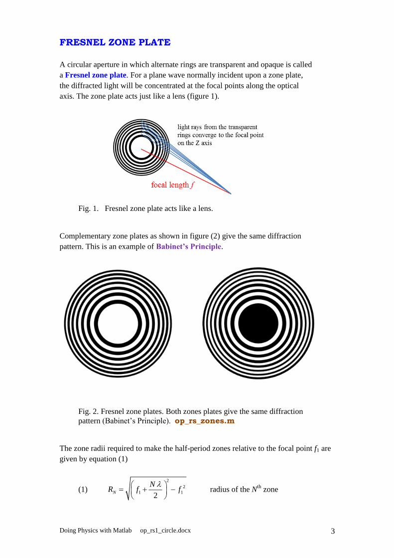
A circular aperture in which alternate rings are transparent and opaque is called

a Fresnel zone plate. For a plane wave normally incident upon a zone plate,

the diffracted light will be concentrated at the focal points along the optical

axis. The zone plate acts just like a lens (figure 1).

Fig. 1. Fresnel zone plate acts like a lens.

Complementary zone plates as shown in figure (2) give the same diffraction

pattern. This is an example of Babinet’s Principle.

Fig. 2. Fresnel zone plates. Both zones plates give the same diffraction

pattern (Babinet’s Principle). op_rs_zones.m

The zone radii required to make the half-period zones relative to the focal point f1 are

given by equation (1)

(1)

2

2

1 12

N

NR f f

radius of the N

th zone

Doing Physics with Matlab op_rs1_circle.docx 4

There are other maximum irradiance points along the optical axis and these focal

points are found at

(2) 2 2

1 11 1

1 11,2, 3,

2 1 2 1m

R Rf f m f

m m

Hence, these focal points occur along the optical axis at zP = f1, f1 / 3, f1 / 5, … .

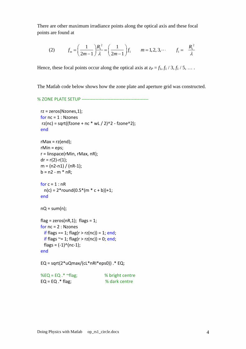
The Matlab code below shows how the zone plate and aperture grid was constructed.

% ZONE PLATE SETUP -------------------------------------------- rz = zeros(Nzones,1); for nc = 1 : Nzones rz(nc) = sqrt((fzone + nc * wL / 2)^2 - fzone^2); end rMax = rz(end); rMin = eps; r = linspace(rMin, rMax, nR); dr = r(2)-r(1); m = (n2-n1) / (nR-1); b = n2 - m * nR; for c = 1 : nR n(c) = 2*round(0.5*(m * c + b))+1; end nQ = sum(n); flag = zeros(nR,1); flags = 1; for nc = 2 : Nzones if flags == 1; flag(r > rz(nc)) = 1; end; if flags ~= 1; flag(r > rz(nc)) = 0; end; flags = (-1)^(nc-1); end EQ = sqrt(2*uQmax/(cL*nRI*eps0)) .* EQ; %EQ = EQ .* ~flag; % bright centre EQ = EQ .* flag; % dark centre

Doing Physics with Matlab op_rs1_circle.docx 5

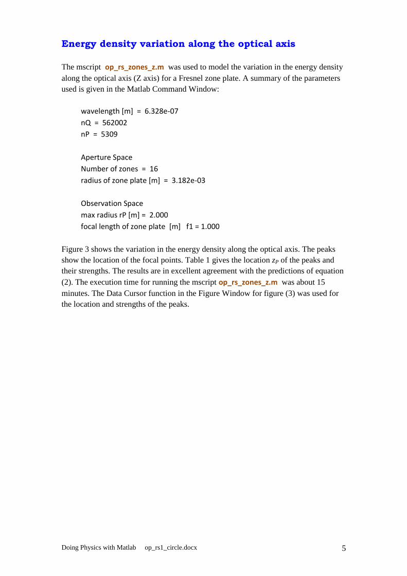
Energy density variation along the optical axis

The mscript op_rs_zones_z.m was used to model the variation in the energy density

along the optical axis (Z axis) for a Fresnel zone plate. A summary of the parameters

used is given in the Matlab Command Window:

wavelength [m] = 6.328e-07

nQ = 562002

nP = 5309

Aperture Space

Number of zones = 16

radius of zone plate [m] = 3.182e-03

Observation Space

max radius rP [m] = 2.000

focal length of zone plate [m] f1 = 1.000

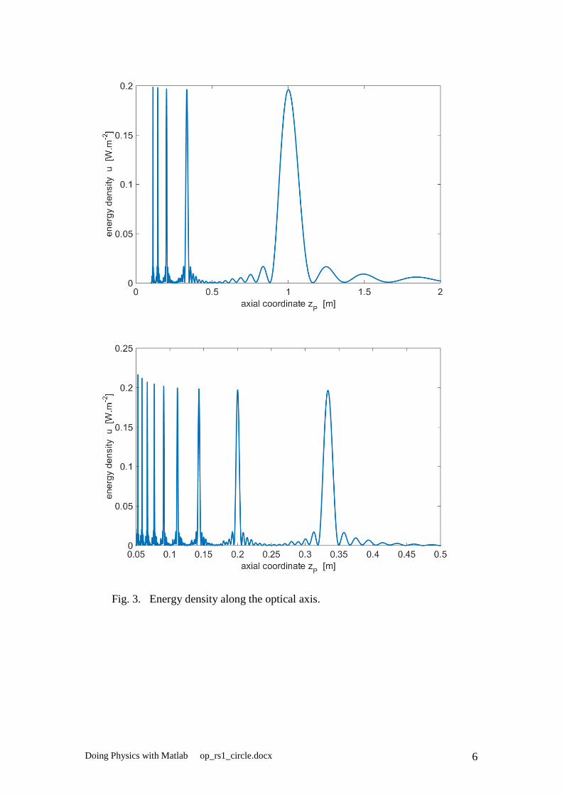
Figure 3 shows the variation in the energy density along the optical axis. The peaks

show the location of the focal points. Table 1 gives the location zP of the peaks and

their strengths. The results are in excellent agreement with the predictions of equation

(2). The execution time for running the mscript op_rs_zones_z.m was about 15

minutes. The Data Cursor function in the Figure Window for figure (3) was used for

the location and strengths of the peaks.

Doing Physics with Matlab op_rs1_circle.docx 6

Fig. 3. Energy density along the optical axis.

Doing Physics with Matlab op_rs1_circle.docx 7

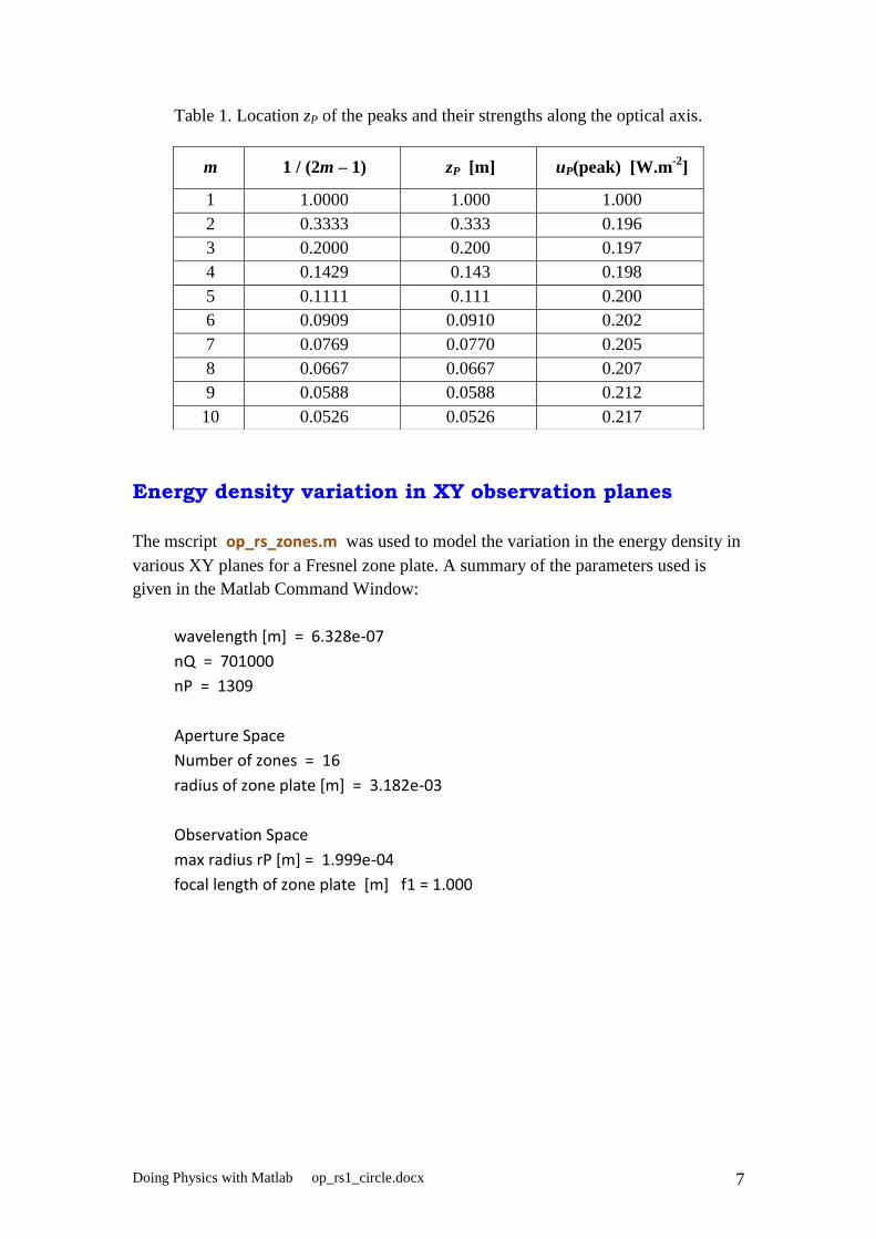
Table 1. Location zP of the peaks and their strengths along the optical axis.

Energy density variation in XY observation planes

The mscript op_rs_zones.m was used to model the variation in the energy density in

various XY planes for a Fresnel zone plate. A summary of the parameters used is

given in the Matlab Command Window:

wavelength [m] = 6.328e-07

nQ = 701000

nP = 1309

Aperture Space

Number of zones = 16

radius of zone plate [m] = 3.182e-03

Observation Space

max radius rP [m] = 1.999e-04

focal length of zone plate [m] f1 = 1.000

m 1 / (2m – 1) zP [m] uP(peak) [W.m-2

]

1 1.0000 1.000 1.000

2 0.3333 0.333 0.196

3 0.2000 0.200 0.197

4 0.1429 0.143 0.198

5 0.1111 0.111 0.200

6 0.0909 0.0910 0.202

7 0.0769 0.0770 0.205

8 0.0667 0.0667 0.207

9 0.0588 0.0588 0.212

10 0.0526 0.0526 0.217

Doing Physics with Matlab op_rs1_circle.docx 8

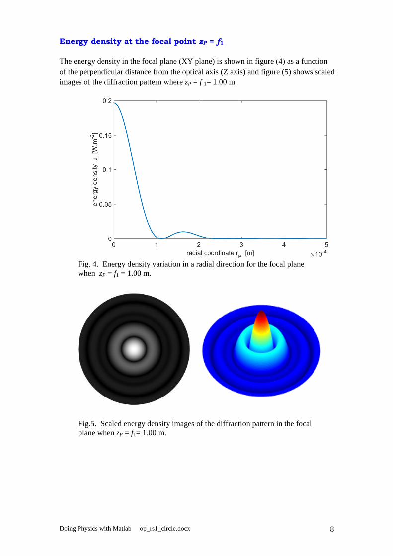
Energy density at the focal point zP = f1

The energy density in the focal plane (XY plane) is shown in figure (4) as a function

of the perpendicular distance from the optical axis (Z axis) and figure (5) shows scaled

images of the diffraction pattern where zP = f 1= 1.00 m.

Fig. 4. Energy density variation in a radial direction for the focal plane

when zP = f1 = 1.00 m.

Fig.5. Scaled energy density images of the diffraction pattern in the focal

plane when zP = f1= 1.00 m.

Doing Physics with Matlab op_rs1_circle.docx 9

The energy density in a XY plane where zP > f1 is shown in figure (6) as

a function of the perpendicular distance from the optical axis (Z axis) and

figure (7) show scaled images of the diffraction pattern where f1 = 1.00 m

and zP = 1.10 m.

Fig. 6. Energy density variation in a radial direction when zP > f1,

f1 = 1.00 m and zP = 1.10 m.

Fig. 7. Scaled energy density images of the diffraction pattern in the

focal plane when zP > f1, f1 = 1.00 m and zP = 1.10 m.

Doing Physics with Matlab op_rs1_circle.docx 10

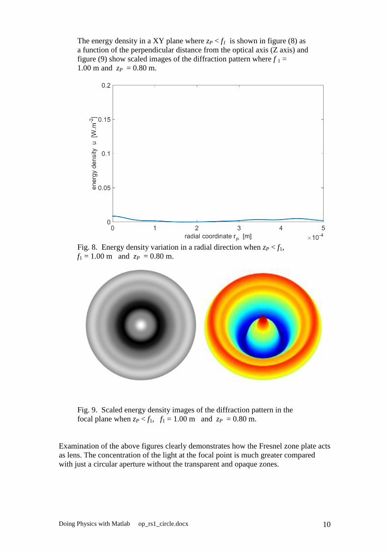
The energy density in a XY plane where zP < f1 is shown in figure (8) as

a function of the perpendicular distance from the optical axis (Z axis) and

figure (9) show scaled images of the diffraction pattern where f 1 =

1.00 m and zP = 0.80 m.

Fig. 8. Energy density variation in a radial direction when zP < f1,

f1 = 1.00 m and zP = 0.80 m.

Fig. 9. Scaled energy density images of the diffraction pattern in the

focal plane when zP < f1, f1 = 1.00 m and zP = 0.80 m.

Examination of the above figures clearly demonstrates how the Fresnel zone plate acts

as lens. The concentration of the light at the focal point is much greater compared

with just a circular aperture without the transparent and opaque zones.

Doing Physics with Matlab op_rs1_circle.docx 11

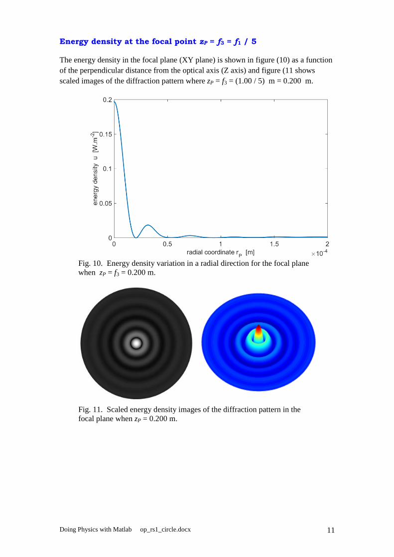
Energy density at the focal point zP = f3 = f1 / 5

The energy density in the focal plane (XY plane) is shown in figure (10) as a function

of the perpendicular distance from the optical axis (Z axis) and figure (11 shows

scaled images of the diffraction pattern where zP = f3 = (1.00 / 5) m = 0.200 m.

Fig. 10. Energy density variation in a radial direction for the focal plane

when zP = f3 = 0.200 m.

Fig. 11. Scaled energy density images of the diffraction pattern in the

focal plane when zP = 0.200 m.

Doing Physics with Matlab op_rs1_circle.docx 12

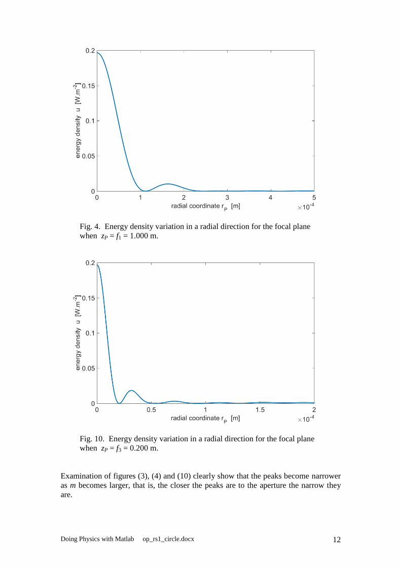
Fig. 4. Energy density variation in a radial direction for the focal plane

when zP = f1 = 1.000 m.

Fig. 10. Energy density variation in a radial direction for the focal plane

when zP = f3 = 0.200 m.

Examination of figures (3), (4) and (10) clearly show that the peaks become narrower

as m becomes larger, that is, the closer the peaks are to the aperture the narrow they

are.