doing physics with matlab computational optics · doing physics with matlab computational optics...
TRANSCRIPT
Doing Physics with Matlab op_rs1_rxy_01.docx 1
DOING PHYSICS WITH MATLAB
COMPUTATIONAL OPTICS
RAYLEIGH-SOMMERFELD DIFFRACTION RECTANGULAR APERTURES
Ian Cooper
School of Physics, University of Sydney
DOWNLOAD DIRECTORY FOR MATLAB SCRIPTS
op_rs_rxy_01.m Calculation of the irradiance in a plane perpendicular to the optical axis for a
uniformly illuminated rectangular aperture.
simpsonxy_coeff.m Function to calculate Simpson’s two-dimensional coefficients
fn_distancePQ.m Function to calculate distance between two points
turningPoints.m Function to find the zero crossings of a function and its maxima and minima
op_rs_rxy_02.m
Updated version of op_rs_rxy_01.m. Calculation of the irradiance in a plane
perpendicular to the optical axis for a rectangular aperture. The irradiance is not
scaled but calculated in W.m-2
. The energy per second from the aperture to the
observation screen is calculated and the energy per second within a circle of radius
equal to the position of the first minima in the X direction in the observation screen is
also calculated.
simpson2d.m Function to calculate the value of a two-dimensional integral using the
Simpson’s [2D] method.
fn_distancePQ.m Function to calculate distance between two points
Doing Physics with Matlab op_rs1_rxy_01.docx 2
FRAUNHOFER DIFFRACTION – RECTANGULAR APERTURE
We will consider the Fraunhofer diffraction patterns for a single rectangular aperture
that is uniformly illuminated. The X and Y widths the rectangular aperture are ax and
ay respectively. The irradiance distribution I is given by the product of two single slit
functions
(1)
22sin( )sin( ) PyPx
o
P x P y
vvI I
v v
Fraunhofer diffraction
where I0 is a normalizing constant and the optical coordinates vPx and vPy are
(2) 1 12 2
sin sin sin sinP x x x x x P y y y y yv k a a v k a a
and the angles x and y define the direction of the diffracted ray
(3) 2 2 2 2
sin sinP Px y
P P P P
x y
x z y z
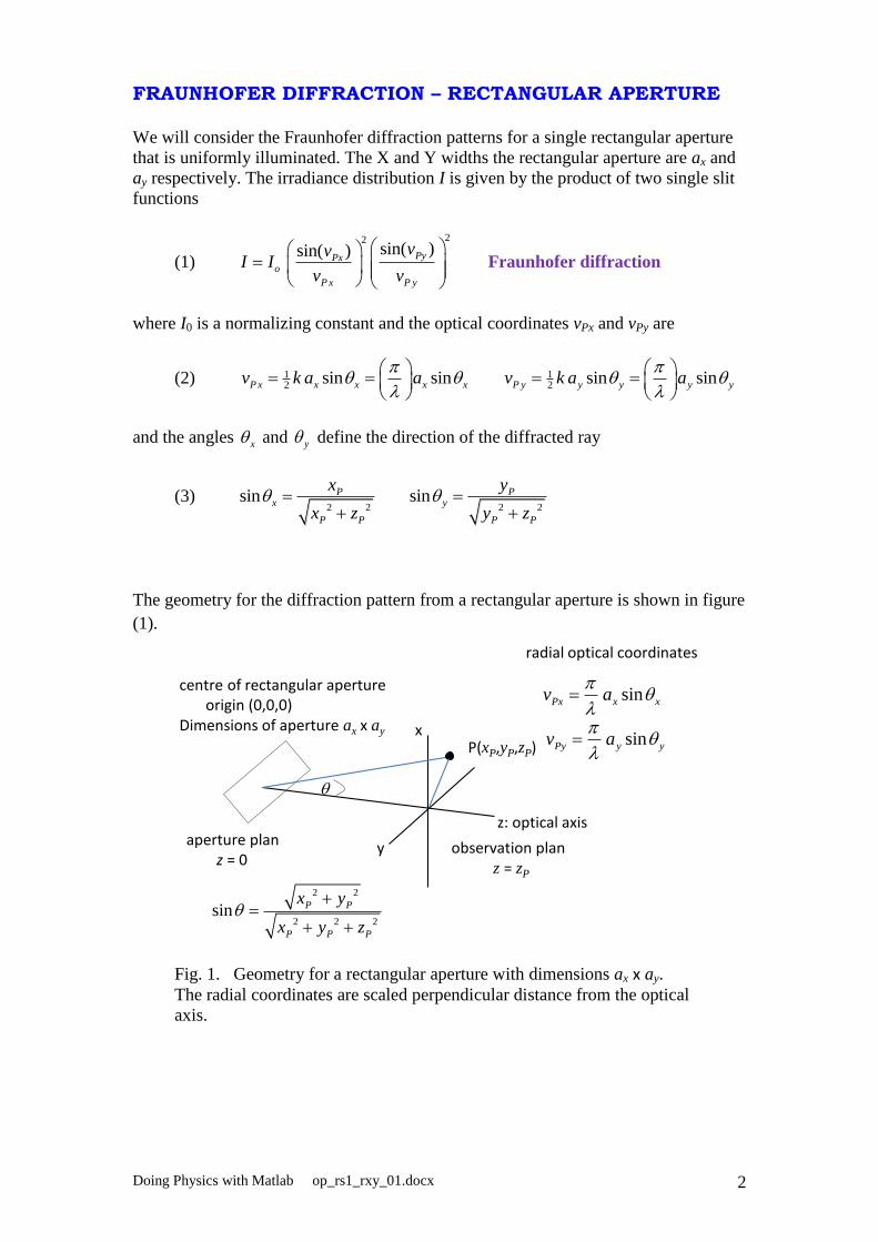
The geometry for the diffraction pattern from a rectangular aperture is shown in figure
(1).
Fig. 1. Geometry for a rectangular aperture with dimensions ax x ay.
The radial coordinates are scaled perpendicular distance from the optical
axis.
z: optical axis
x
y
centre of rectangular apertureorigin (0,0,0)
Dimensions of aperture ax x ay
P(xP,yP,zP)
aperture planz = 0
observation planz = zP
2 2
2 2 2sin P P
P P P
x y
x y z
sinPx x xv a
radial optical coordinates
sinPy y yv a
Doing Physics with Matlab op_rs1_rxy_01.docx 3
The resulting diffraction pattern for the irradiance has lines of zeros when
(3a) 1, 2, 3,Px x xv m m and 1, 2, 3,P y y yv m m
or
(3b) sin sinx x x y y ym a m a
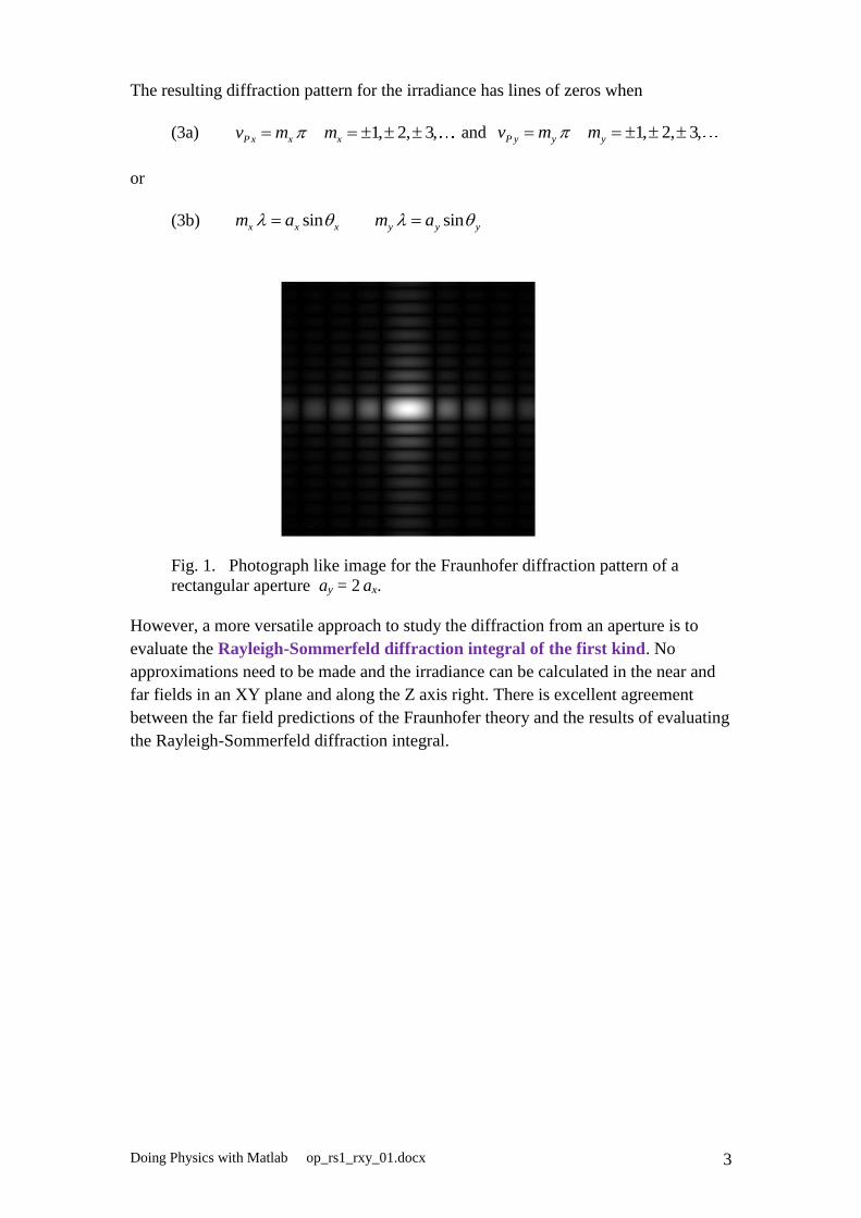
Fig. 1. Photograph like image for the Fraunhofer diffraction pattern of a
rectangular aperture ay = 2 ax.
However, a more versatile approach to study the diffraction from an aperture is to
evaluate the Rayleigh-Sommerfeld diffraction integral of the first kind. No
approximations need to be made and the irradiance can be calculated in the near and
far fields in an XY plane and along the Z axis right. There is excellent agreement
between the far field predictions of the Fraunhofer theory and the results of evaluating
the Rayleigh-Sommerfeld diffraction integral.
Doing Physics with Matlab op_rs1_rxy_01.docx 4
RAYLEIGH DIFFRACTION INTEGRAL OF THE FIRST KIND
The Rayleigh-Sommerfeld region includes the entire space to the right of the
aperture. It is assumed that the Rayleigh-Sommerfeld diffraction integral of the first
kind is valid throughout this space, right down to the aperture. There are no
limitations on the maximum size of either the aperture or observation region, relative
to the observation distance, because no approximations have been made.
The Rayleigh-Sommerfeld diffraction integral of the first kind (RS1) can be expressed
as
(4)
A
3
1( 1) d
2
PQj k r
P Q p PQ
PQS
eE E z j k r S
r
where EP is the electric field at the observation point P, EQ is the electric field within
the aperture and rPQ is the distance from an aperture point Q to the point P. The
double integral is over the area of the aperture SA.
Approach 1 to evaluating The Diffraction Integral
op_rs_rxy_01.m
The double integral can be estimate numerically by a two-dimensional form of
Simpson’s 1/3 rule. The electric field EP at the point P is computed by
(5) 0 31 1
S 1PQmnj k rN N
P mn Qmn Pmn PQmn
m n PQmn
eE E E z j k r
r
where Smn are the Simpson’s two-dimensional coefficients and E0 is a normalizing
constant. Each term in equation (2) can be expressed as a matrix of size N N and
the matrices can be manipulated very easily in Matlab to give the estimate of the
integral. The irradiance is proportional to the square of the magnitude of the electric
field, hence the irradiance in the space beyond the aperture can be calculated by
(6) *
0I I E E
where I0 is a normalizing constant and E* is the complex conjugate of E.
Doing Physics with Matlab op_rs1_rxy_01.docx 5
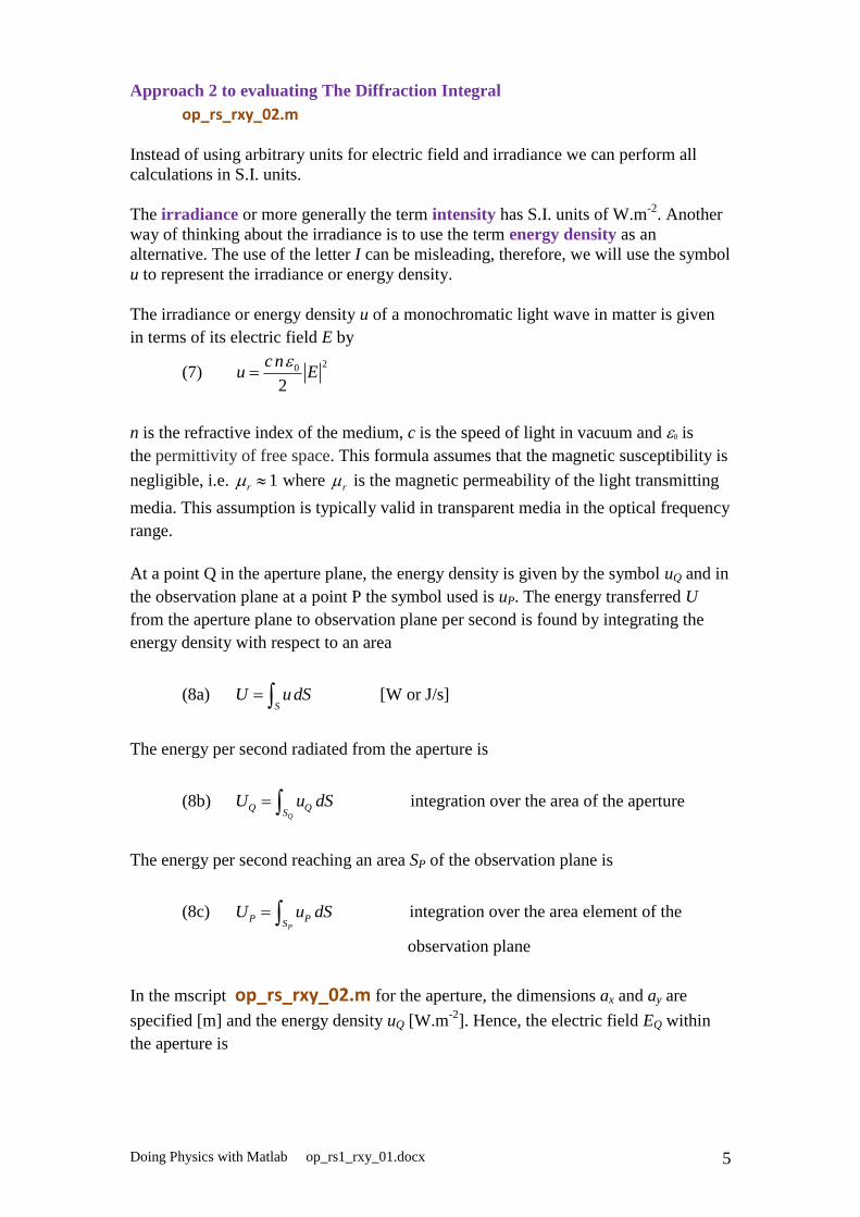
Approach 2 to evaluating The Diffraction Integral
op_rs_rxy_02.m
Instead of using arbitrary units for electric field and irradiance we can perform all
calculations in S.I. units.
The irradiance or more generally the term intensity has S.I. units of W.m-2
. Another
way of thinking about the irradiance is to use the term energy density as an
alternative. The use of the letter I can be misleading, therefore, we will use the symbol
u to represent the irradiance or energy density.
The irradiance or energy density u of a monochromatic light wave in matter is given
in terms of its electric field E by
(7) 20
2
c nu E
n is the refractive index of the medium, c is the speed of light in vacuum and 0 is
the permittivity of free space. This formula assumes that the magnetic susceptibility is
negligible, i.e. 1r where r is the magnetic permeability of the light transmitting
media. This assumption is typically valid in transparent media in the optical frequency
range.
At a point Q in the aperture plane, the energy density is given by the symbol uQ and in
the observation plane at a point P the symbol used is uP. The energy transferred U
from the aperture plane to observation plane per second is found by integrating the
energy density with respect to an area
(8a) S
U u dS [W or J/s]
The energy per second radiated from the aperture is
(8b) Q
Q QS
U u dS integration over the area of the aperture
The energy per second reaching an area SP of the observation plane is
(8c) P
P PS
U u dS integration over the area element of the
observation plane
In the mscript op_rs_rxy_02.m for the aperture, the dimensions ax and ay are
specified [m] and the energy density uQ [W.m-2
]. Hence, the electric field EQ within
the aperture is
Doing Physics with Matlab op_rs1_rxy_01.docx 6
(9) 0
2 Q
Q
uE
c n
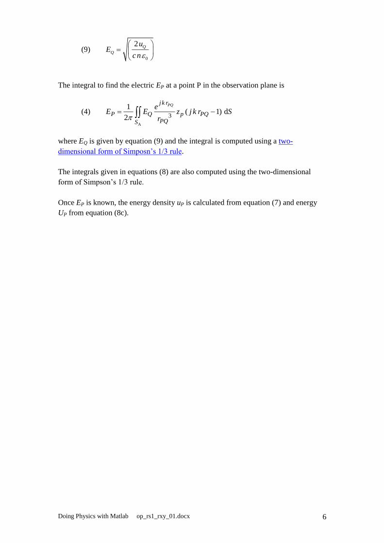
The integral to find the electric EP at a point P in the observation plane is
(4)
A
3
1( 1) d
2
PQj k r
P Q p PQ
PQS
eE E z j k r S
r
where EQ is given by equation (9) and the integral is computed using a two-
dimensional form of Simposn’s 1/3 rule.
The integrals given in equations (8) are also computed using the two-dimensional
form of Simpson’s 1/3 rule.
Once EP is known, the energy density uP is calculated from equation (7) and energy
UP from equation (8c).
Doing Physics with Matlab op_rs1_rxy_01.docx 7
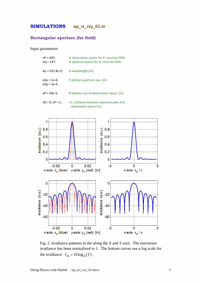
SIMULATIONS op_rs_rxy_01.m
Rectangular aperture (far field)
Input parameters
nP = 495; % observation points for P must be ODD nQ = 147; % aperture points for Q must be ODD wL = 632.8e-9; % wavelength [m] aQx = 1e-4; % defines aperture size [m] aQy = 2e-4; aP = 30e-3; % defines size of observation space [m] zQ = 0; zP = 1; % z distance between aperture plan and observation plane [m]
Fig. 2. Irradiance patterns in the along the X and Y axes. The maximum
irradiance has been normalized to 1. The bottom curves use a log scale for
the irradiance 1010logdBI I .
Doing Physics with Matlab op_rs1_rxy_01.docx 8
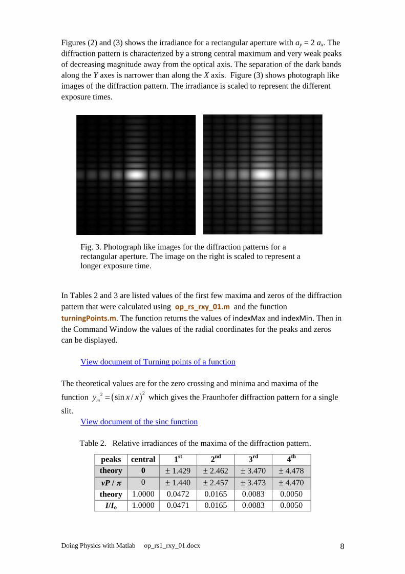
Figures (2) and (3) shows the irradiance for a rectangular aperture with ay = 2 ax. The
diffraction pattern is characterized by a strong central maximum and very weak peaks
of decreasing magnitude away from the optical axis. The separation of the dark bands
along the Y axes is narrower than along the X axis. Figure (3) shows photograph like
images of the diffraction pattern. The irradiance is scaled to represent the different
exposure times.
Fig. 3. Photograph like images for the diffraction patterns for a
rectangular aperture. The image on the right is scaled to represent a
longer exposure time.
In Tables 2 and 3 are listed values of the first few maxima and zeros of the diffraction
pattern that were calculated using op_rs_rxy_01.m and the function
turningPoints.m. The function returns the values of indexMax and indexMin. Then in
the Command Window the values of the radial coordinates for the peaks and zeros
can be displayed.
View document of Turning points of a function
The theoretical values are for the zero crossing and minima and maxima of the
function 22 sin /my x x which gives the Fraunhofer diffraction pattern for a single
slit.
View document of the sinc function
Table 2. Relative irradiances of the maxima of the diffraction pattern.
peaks central 1st 2
nd 3
rd 4
th
theory 0 1.429 2.462 3.470 4.478
vP / 0 1.440 2.457 3.473 4.470
theory 1.0000 0.0472 0.0165 0.0083 0.0050
I/Io 1.0000 0.0471 0.0165 0.0083 0.0050
Doing Physics with Matlab op_rs1_rxy_01.docx 9
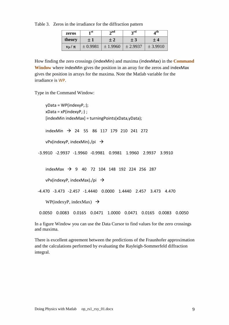
Table 3. Zeros in the irradiance for the diffraction pattern
How finding the zero crossings (indexMin) and maxima (indexMax) in the Command
Window where indexMin gives the position in an array for the zeros and indexMax
gives the position in arrays for the maxima. Note the Matlab variable for the
irradiance is WP.
Type in the Command Window:
yData = WP(indexyP,:);
xData = xP(indexyP,:) ;
[indexMin indexMax] = turningPoints(xData,yData);
indexMin 24 55 86 117 179 210 241 272
vPx(indexyP, indexMin)./pi
-3.9910 -2.9937 -1.9960 -0.9981 0.9981 1.9960 2.9937 3.9910
indexMax 9 40 72 104 148 192 224 256 287
vPx(indexyP, indexMax)./pi
-4.470 -3.473 -2.457 -1.4440 0.0000 1.4440 2.457 3.473 4.470
WP(indexyP, indexMax)
0.0050 0.0083 0.0165 0.0471 1.0000 0.0471 0.0165 0.0083 0.0050 In a figure Window you can use the Data Cursor to find values for the zero crossings
and maxima.
There is excellent agreement between the predictions of the Fraunhofer approximation
and the calculations performed by evaluating the Rayleigh-Sommerfeld diffraction
integral.
zeros 1st 2
nd 3
rd 4
th
theory 1 2 3 4
vP / 0.9981 1.9960 2.9937 3.9910
Doing Physics with Matlab op_rs1_rxy_01.docx 10
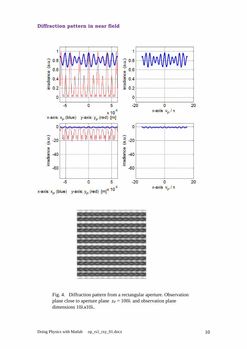
Diffraction pattern in near field
Fig. 4. Diffraction pattern from a rectangular aperture. Observation
plane close to aperture plane zP = 100 and observation plane
dimensions 10x10.
Doing Physics with Matlab op_rs1_rxy_01.docx 11
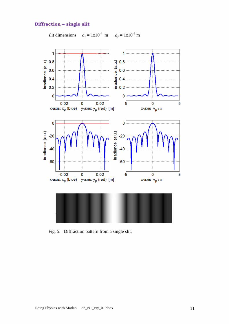
Diffraction – single slit
slit dimensions ax = 1x10⁻⁴
m ay = 1x10⁻⁶
m
Fig. 5. Diffraction pattern from a single slit.
Doing Physics with Matlab op_rs1_rxy_01.docx 12
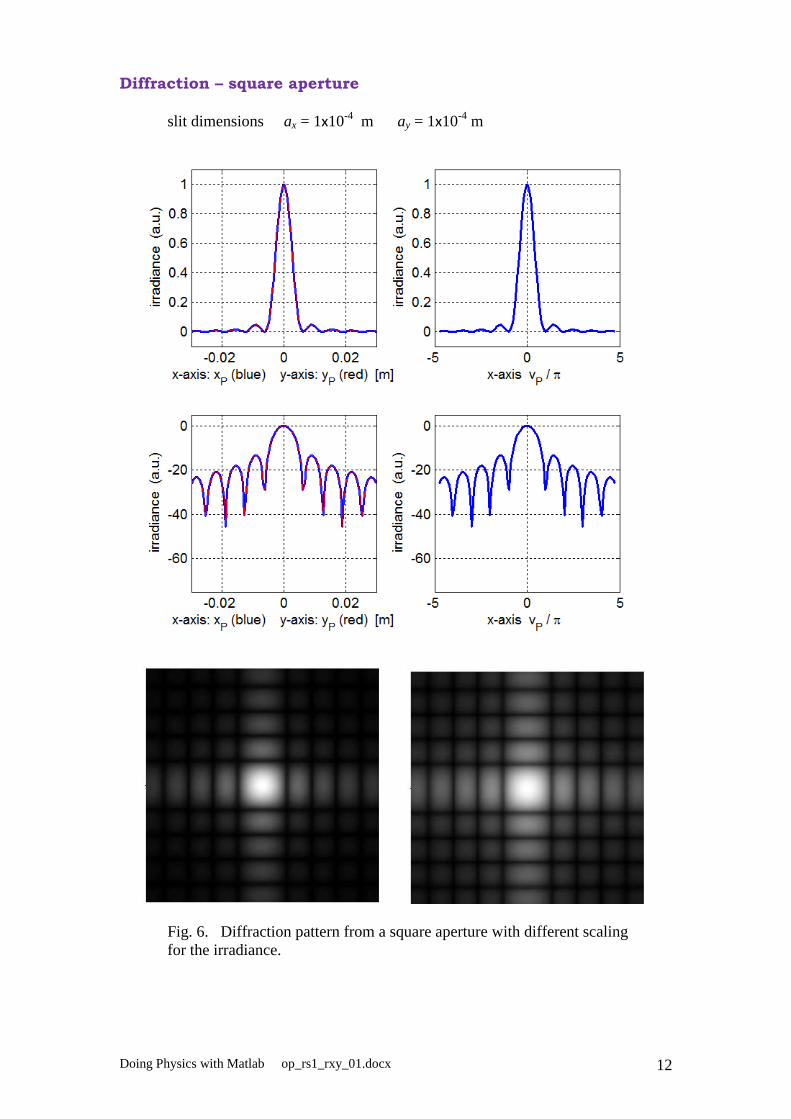
Diffraction – square aperture
slit dimensions ax = 1x10⁻⁴
m ay = 1x10⁻⁴
m
Fig. 6. Diffraction pattern from a square aperture with different scaling
for the irradiance.
Doing Physics with Matlab op_rs1_rxy_01.docx 13
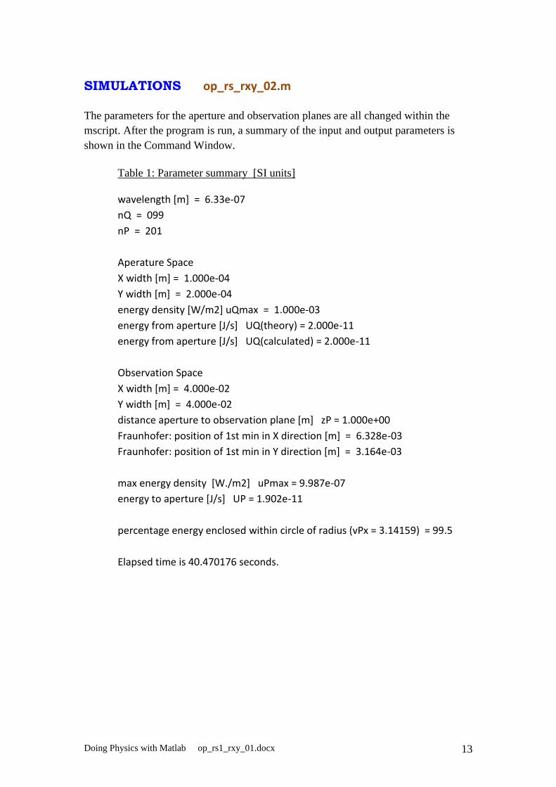
SIMULATIONS op_rs_rxy_02.m
The parameters for the aperture and observation planes are all changed within the
mscript. After the program is run, a summary of the input and output parameters is
shown in the Command Window.
Table 1: Parameter summary [SI units]
wavelength [m] = 6.33e-07
nQ = 099
nP = 201
Aperature Space
X width [m] = 1.000e-04
Y width [m] = 2.000e-04
energy density [W/m2] uQmax = 1.000e-03
energy from aperture [J/s] UQ(theory) = 2.000e-11
energy from aperture [J/s] UQ(calculated) = 2.000e-11
Observation Space
X width [m] = 4.000e-02
Y width [m] = 4.000e-02
distance aperture to observation plane [m] zP = 1.000e+00
Fraunhofer: position of 1st min in X direction [m] = 6.328e-03
Fraunhofer: position of 1st min in Y direction [m] = 3.164e-03
max energy density [W./m2] uPmax = 9.987e-07
energy to aperture [J/s] UP = 1.902e-11
percentage energy enclosed within circle of radius (vPx = 3.14159) = 99.5
Elapsed time is 40.470176 seconds.
Doing Physics with Matlab op_rs1_rxy_01.docx 14
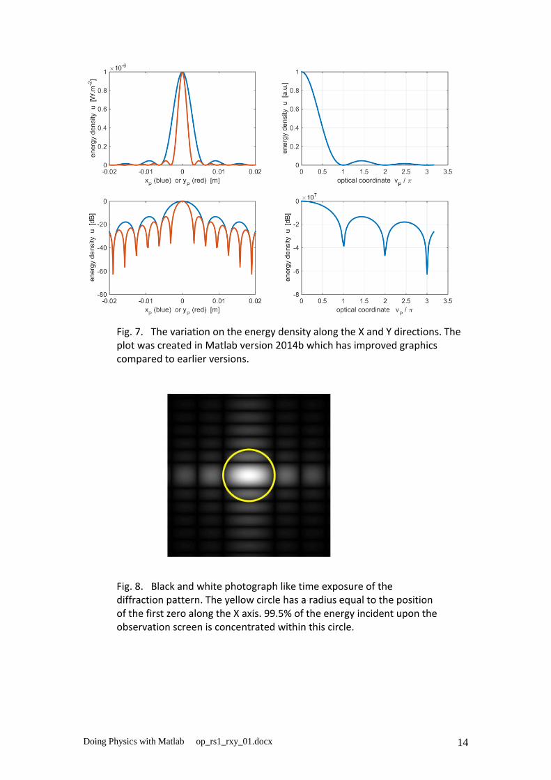
Fig. 7. The variation on the energy density along the X and Y directions. The plot was created in Matlab version 2014b which has improved graphics compared to earlier versions.
Fig. 8. Black and white photograph like time exposure of the diffraction pattern. The yellow circle has a radius equal to the position of the first zero along the X axis. 99.5% of the energy incident upon the observation screen is concentrated within this circle.
Doing Physics with Matlab op_rs1_rxy_01.docx 15
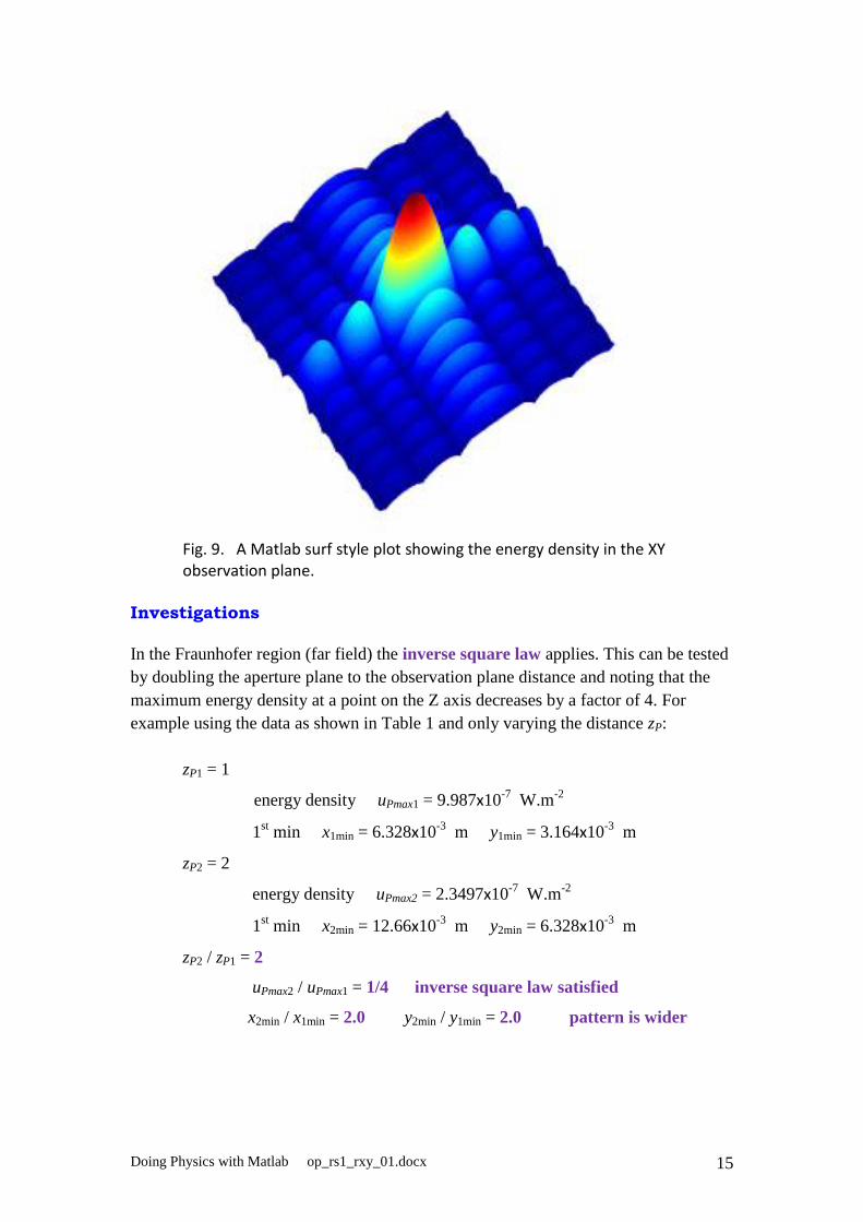
Fig. 9. A Matlab surf style plot showing the energy density in the XY observation plane.
Investigations
In the Fraunhofer region (far field) the inverse square law applies. This can be tested
by doubling the aperture plane to the observation plane distance and noting that the
maximum energy density at a point on the Z axis decreases by a factor of 4. For
example using the data as shown in Table 1 and only varying the distance zP:
zP1 = 1
energy density uPmax1 = 9.987x10⁻⁷
W.m-2
1st min x1min = 6.328x10
-3 m y1min = 3.164x10
-3 m
zP2 = 2
energy density uPmax2 = 2.3497x10⁻⁷
W.m-2
1st min x2min = 12.66x10
-3 m y2min = 6.328x10
-3 m
zP2 / zP1 = 2
uPmax2 / uPmax1 = 1/4 inverse square law satisfied
x2min / x1min = 2.0 y2min / y1min = 2.0 pattern is wider
Doing Physics with Matlab op_rs1_rxy_01.docx 16
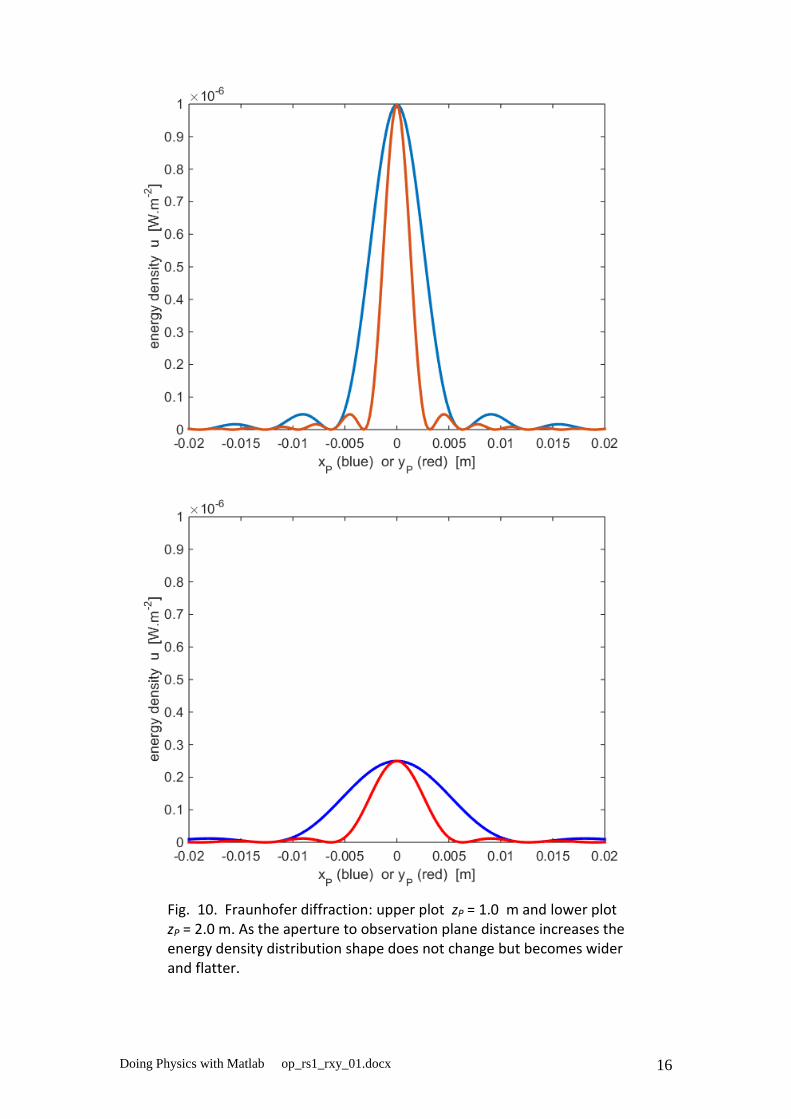
Fig. 10. Fraunhofer diffraction: upper plot zP = 1.0 m and lower plot zP = 2.0 m. As the aperture to observation plane distance increases the energy density distribution shape does not change but becomes wider and flatter.
Doing Physics with Matlab op_rs1_rxy_01.docx 17
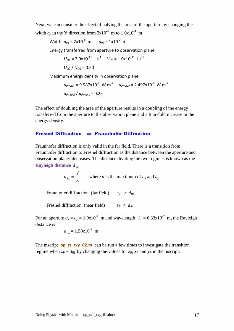
Next, we can consider the effect of halving the area of the aperture by changing the
width ay in the Y direction from 2x10⁻⁴
m to 1.0x10⁻⁴
m.
Width ay1 = 2x10⁻⁴ m ay2 = 1x10⁻² m
Energy transferred from aperture to observation plane
UQ1 = 2.0x10⁻¹¹ J.s-1 UQ2 = 1.0x10⁻¹¹ J.s-1
UQ2 / UQ1 = 0.50
Maximum energy density in observation plane
uPmax1 = 9.987x10⁻⁷ W.m-2 uPmax2 = 2.497x10⁻⁷ W.m-2
uPmax2 / uPmax1 = 0.25
The effect of doubling the area of the aperture results in a doubling of the energy
transferred from the aperture to the observation plane and a four-fold increase in the
energy density.
Fresnel Diffraction Fraunhofer Diffraction
Fraunhofer diffraction is only valid in the far field. There is a transition from
Fraunhofer diffraction to Fresnel diffraction as the distance between the aperture and
observation planes decreases. The distance dividing the two regimes is known as the
Rayleigh distance RLd
2
RL
ad
where a is the maximum of ax and ay
Fraunhofer diffraction (far field) zP > dRL
Fresnel diffraction (near field) zP < dRL
For an aperture ax = ay = 1.0x10⁻⁴
m and wavelength = 6.33x10⁻⁷
m, the Rayleigh
distance is
RLd = 1.58x10⁻²
m
The mscript op_rs_rxy_02.m can be run a few times to investigate the transition
regime when zP ~ dRL by changing the values for zP, xP and yP in the mscript.
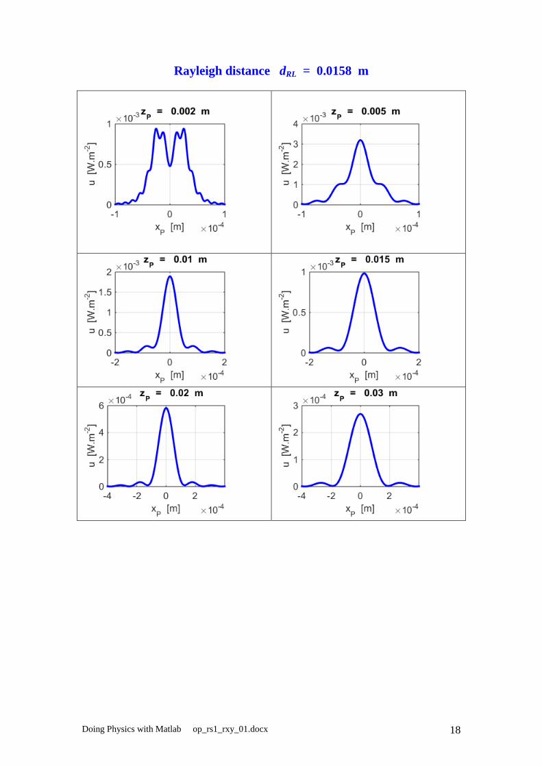
Doing Physics with Matlab op_rs1_rxy_01.docx 18
Rayleigh distance dRL = 0.0158 m