Computational Physics

MATLAB

Peter Hertel

University of Osnabrück, Germany

Matlab is a compact, but powerful language for numerical computations.Matlab is concerned with matrices: rectangular patterns of integer, real, orcomplex numbers. A number itself is a 1 × 1 matrix, a row vector a 1 × npattern, a column an n × 1 matrix. Most Matlab operations affect theentire matrix. Matlab contains and makes available the software treasureof more than 50 years, originally coded in Fortran. Matlab programs,if they avoid repetitive statements, are highly efficient. This introductorycrash course addresses physicists who are used to learn by studying well-chosen examples.

February 18, 2009

Contents

1 Getting startet 3

2 Beijing-Frankfurt 5

3 Avoid loops! 7

4 True, false and NaN 10

5 Functions 13

6 Ordinary differential equations 15

7 Reading and writing data 18

8 Linear Algebra 20

9 Their logo 23

2

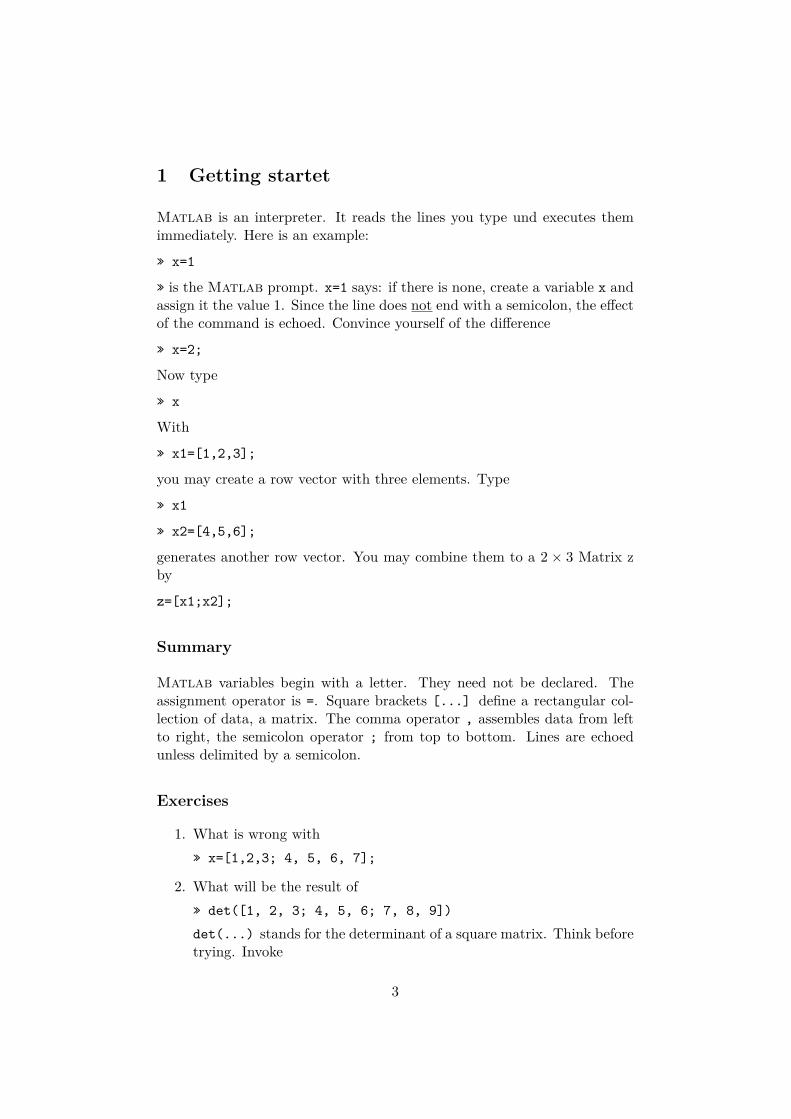
1 Getting startet

Matlab is an interpreter. It reads the lines you type und executes themimmediately. Here is an example:

» x=1

» is the Matlab prompt. x=1 says: if there is none, create a variable x andassign it the value 1. Since the line does not end with a semicolon, the effectof the command is echoed. Convince yourself of the difference

» x=2;

Now type

» x

With

» x1=[1,2,3];

you may create a row vector with three elements. Type

» x1

» x2=[4,5,6];

generates another row vector. You may combine them to a 2 × 3 Matrix zby

z=[x1;x2];

Summary

Matlab variables begin with a letter. They need not be declared. Theassignment operator is =. Square brackets [...] define a rectangular col-lection of data, a matrix. The comma operator , assembles data from leftto right, the semicolon operator ; from top to bottom. Lines are echoedunless delimited by a semicolon.

Exercises

1. What is wrong with» x=[1,2,3; 4, 5, 6, 7];

2. What will be the result of» det([1, 2, 3; 4, 5, 6; 7, 8, 9])

det(...) stands for the determinant of a square matrix. Think beforetrying. Invoke

3

» help det

or» helpdesk

for further details.

3. Try» x=pi

» x=i

4. The same with» format long;

5. Compare» a=[[1;2],[3;4],[5;6]]

with» b=[[1,3,5];[2,4,6]]

4

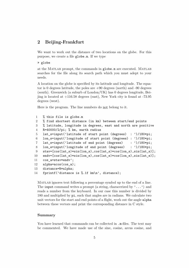
2 Beijing-Frankfurt

We want to work out the distance of two locations on the globe. For thispurpose, we create a file globe.m. If we type

» globe

at the Matlab prompt, the commands in globe.m are executed. Matlabsearches for the file along its search path which you must adept to yourneeds.

A location on the globe is specified by its latitude and longitude. The equa-tor is 0 degrees latitude, the poles are +90 degrees (north) and -90 degrees(south). Greenwich (a suburb of London/UK) has 0 degrees longitude, Bei-jing is located at +116.58 degrees (east), New York city is found at -73.95degrees (west).

Here is the program. The line numbers do not belong to it.

1 % this file is globe.m2 % find shortest distance (in km) between start/end points3 % latitude, longitude in degrees, east and north are positive4 R=40000/2/pi; % km, earth radius5 lat_s=input(’latitude of start point (degrees) : ’)/180*pi;6 lon_s=input(’longitude of start point (degrees) : ’)/180*pi;7 lat_e=input(’latitude of end point (degrees) : ’)/180*pi;8 lon_e=input(’longitude of end point (degrees) : ’)/180*pi;9 stav=[cos(lat_s)*sin(lon_s),cos(lat_s)*cos(lon_s),sin(lat_s)];10 endv=[cos(lat_e)*sin(lon_e),cos(lat_e)*cos(lon_e),sin(lat_e)];11 cos_a=stav*endv’;12 alpha=acos(cos_a);13 distance=R*alpha;14 fprintf(’distance is %.1f km\n’, distance);

Matlab ignores text following a percentage symbol up to the end of a line.The input command writes a prompt (a string, characerized by ’...’) andreads a number from the keyboard. In our case this number is divided by180 and multiplied by pi, such that angles are in radians. We calculate twounit vectors for the start and end points of a flight, work out the angle alphabetween these vectors and print the corresponding distance in C style.

Summary

You have learned that commands can be collected in .m-files. The text maybe commented. We have made use of the sine, cosine, arcus cosine, and

5

fprintf functions. The scalar product of two row vectors a and b is denotedby a*b’; the dash operator denoting transposing (interchanging the meaningof rows and columns).

Exercises

1. Rewrite the above program such that the input can be specified indegrees and minutes.

2. Find out the reaction to erroneous input.

3. Play with the fprintf statement.

4. Replace the fourfold /180*pi statement by something better.

5. Calculate the shortest distance between Beijing = [40.05, 116.58] andFrankfurt/Main = [50.03, 8.55].

6

3 Avoid loops!

Assume you want to plot the sine function. In a traditional programminglanguage, you would write something like

1 N=1023;2 x,y = ARRAY [0..N] of REAL;3 step:=2*pi/N;4 for i:=0 to N do5 x[i]:=i*step;6 y[i]:=sin(x[i]);7 end;

The same in Matlab:

» x=linspace(0,2*pi,1024);

» y=sin(x);

We refrain from showing a dull sine curve which you may obtain by typing

» plot(x,sin(x));

We consider x to be a variable within the interval [0, 2π], but since we workon a machine with a finite number of states only, the variable must becharacterized by representative values, here 1024. The function linspacegenerates a row vector of equally spaced values. The first two argumentsdenote the begin and end of the interval, the third the number of represen-tative points. If x is a matrix, then sin(x) denotes an array of the samedimension, with each component of x being replaced by its sine.

The operators + and - work as expected, they work on matrices component-wise. However,

» x=[1,2,3;4,5,6];

» y=[7,8;9,10;11,12];

» z=x*y

produces [58,64;139,154] which is obviously the result of matrix multi-plication.

However, if you have two matrices of the same format, you may multiplythem componentwise by the .* operator (dot multiplication). The sameholds true for component-wise division by the ./ operator.

You should avoid for-loops whenever you can. To demonstrate this, wegenerate two matrices of normally distributed random numbers and multiplythem, first in the Matlab style.

7

1 a=randn(100,100);2 b=randn(100,100);3 tic;4 c=a*b;5 toc;

And now the same in the old style:

1 a=randn(100,100);2 b=randn(100,100);3 tic;4 for i=1:1005 for k=1:1006 sum=0;7 for j=1:1008 sum=sum+a(i,j)*b(j,k);9 end;10 c(i,k)=sum;11 end;12 end;13 toc;

Although formally correct, the second version requires 50 seconds (on mylaptop), the first is done within 0.11 seconds. You see the difference?

Summary

Most Matlab operators or functions work on entire matrices. for-loopscan usually be avoided.

Exercises

1. What are the execution times of the above two matrix multiplicationprograms on your machine?

2. Generate a column vector r=randn(10000,1) of 10000 normally dis-tributed random numbers and generate its sum by sum(r). What doyou expect? Note that N normally distributed numbers tend to addup to zero. The deviation is of order

√N . Try once more, or even

better: r=randn(10000,10) and sum(r).

3. Generate two 2 × 2 matrices and demonstrate the difference betweenc=a*b and c=a.*b.

8

4. Generate two row vectors vectors a and b of normally distributed ran-dom number and work out their scalar product s=a*b’. Explore a*band a’*b as well.

5. Call the Matlab help system to find out the difference between randand randn.

6. Make yourself acquainted with tic and toc.

9

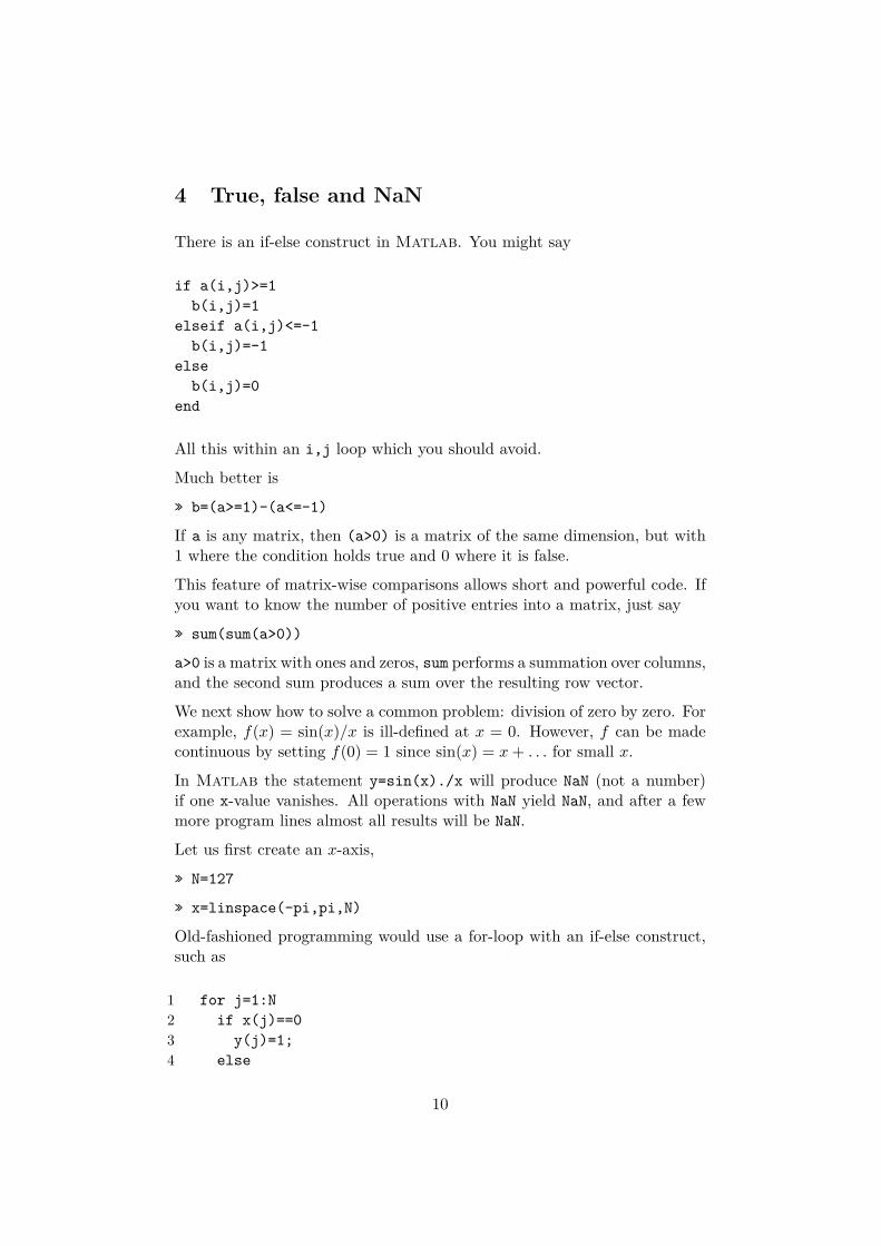
4 True, false and NaN

There is an if-else construct in Matlab. You might say

if a(i,j)>=1b(i,j)=1

elseif a(i,j)<=-1b(i,j)=-1

elseb(i,j)=0

end

All this within an i,j loop which you should avoid.

Much better is

» b=(a>=1)-(a<=-1)

If a is any matrix, then (a>0) is a matrix of the same dimension, but with1 where the condition holds true and 0 where it is false.

This feature of matrix-wise comparisons allows short and powerful code. Ifyou want to know the number of positive entries into a matrix, just say

» sum(sum(a>0))

a>0 is a matrix with ones and zeros, sum performs a summation over columns,and the second sum produces a sum over the resulting row vector.

We next show how to solve a common problem: division of zero by zero. Forexample, f(x) = sin(x)/x is ill-defined at x = 0. However, f can be madecontinuous by setting f(0) = 1 since sin(x) = x+ . . . for small x.

In Matlab the statement y=sin(x)./x will produce NaN (not a number)if one x-value vanishes. All operations with NaN yield NaN, and after a fewmore program lines almost all results will be NaN.

Let us first create an x-axis,

» N=127

» x=linspace(-pi,pi,N)

Old-fashioned programming would use a for-loop with an if-else construct,such as

1 for j=1:N2 if x(j)==03 y(j)=1;4 else

10

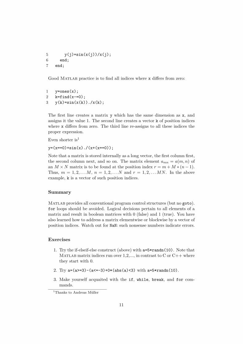
5 y(j)=sin(x(j))/x(j);6 end;7 end;

Good Matlab practice is to find all indices where x differs from zero:

1 y=ones(x);2 k=find(x~=0);3 y(k)=sin(x(k))./x(k);

The first line creates a matrix y which has the same dimension as x, andassigns it the value 1. The second line creates a vector k of position indiceswhere x differs from zero. The third line re-assigns to all these indices theproper expression.

Even shorter is1

y=(x==0)+sin(x)./(x+(x==0));

Note that a matrix is stored internally as a long vector, the first column first,the second column next, and so on. The matrix element amn = a(m,n) ofan M ×N matrix is to be found at the position index r = m+M ∗ (n− 1).Thus, m = 1, 2, . . .M , n = 1, 2, . . . N and r = 1, 2, . . .MN . In the aboveexample, k is a vector of such position indices.

Summary

Matlab provides all conventional program control structures (but no goto).for loops should be avoided. Logical decisions pertain to all elements of amatrix and result in boolean matrices with 0 (false) and 1 (true). You havealso learned how to address a matrix elementwise or blockwise by a vector ofposition indices. Watch out for NaN: such nonsense numbers indicate errors.

Exercises

1. Try the if-elseif-else construct (above) with a=5*randn(10). Note thatMatlab matrix indices run over 1,2,..., in contrast to C or C++ wherethey start with 0.

2. Try a=(a>=3)-(a<=-3)+0*(abs(a)<3) with a=5*randn(10).

3. Make yourself acquaited with the if, while, break, and for com-mands.

1Thanks to Andreas Müller

11

4. Generate two matrices a and b and play with ~ (not), == (equal), <=(smaller than or equal), > (larger than), ~= (not equal), & (and), | (or)etc.

5. Work out y = sin(x)/x by

• » y=sin(x)./x;

• » y=(x==0)+(x~=0).*sin(x)./x;

• with for and if-else

• using the find function

and check for NaN.

6. What do you expect?» a=randn(4);

» k=find(a==nan)

7. Convince yourself that a number, as assigned by» x=7

can be addressed as» x(1,1)

or» x(1)

or» x

The two index form is correct since everything in Matlab is a matrix.The one index form refers to the storage method. The no index formis a for ease of usage.

12

5 Functions

Assume a continuous real valued function f = f(x) depending on one realvariable. The definite integral

∫ ba f(x)dx is well defined. Here we are not

concerned with numerical quadrature, or integration methods. The prob-lem is how to formulate a function in Matlab. There is a large group offunctions which take functions as an argument. In the help system they aregrouped as ’funfun’, a funny pun.

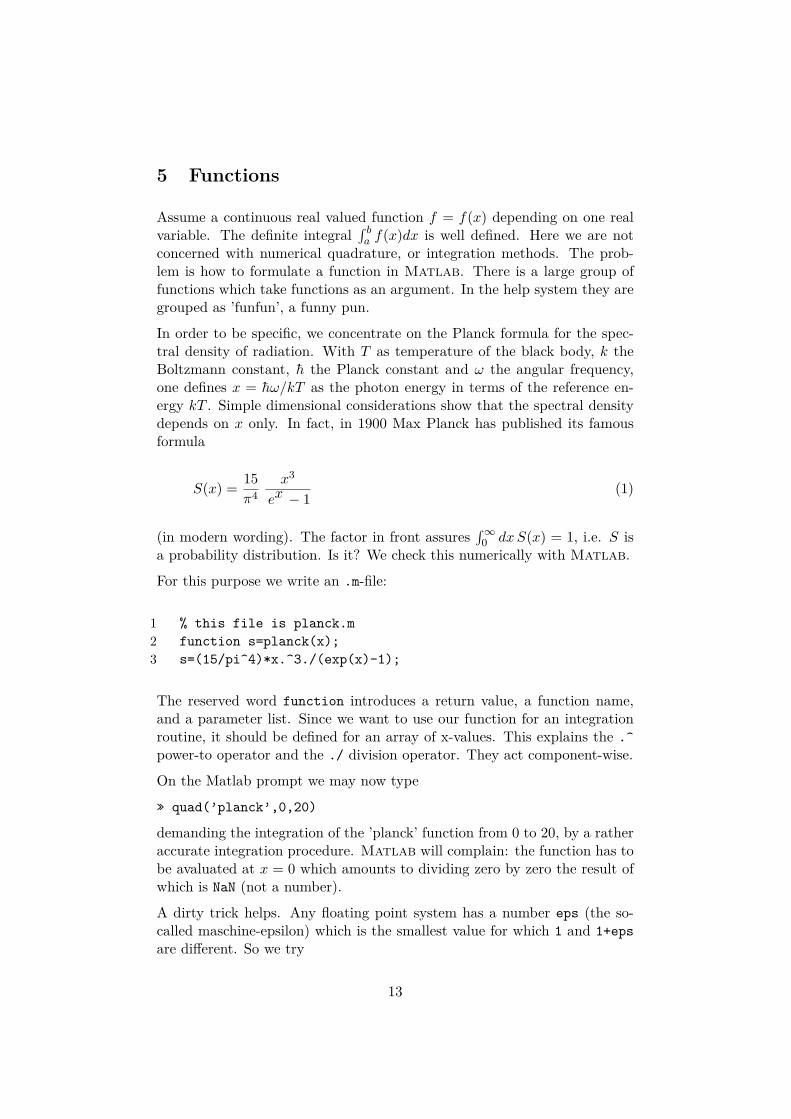
In order to be specific, we concentrate on the Planck formula for the spec-tral density of radiation. With T as temperature of the black body, k theBoltzmann constant, h the Planck constant and ω the angular frequency,one defines x = hω/kT as the photon energy in terms of the reference en-ergy kT . Simple dimensional considerations show that the spectral densitydepends on x only. In fact, in 1900 Max Planck has published its famousformula

S(x) = 15π4

x3

ex − 1(1)

(in modern wording). The factor in front assures∫∞

0 dxS(x) = 1, i.e. S isa probability distribution. Is it? We check this numerically with Matlab.

For this purpose we write an .m-file:

1 % this file is planck.m2 function s=planck(x);3 s=(15/pi^4)*x.^3./(exp(x)-1);

The reserved word function introduces a return value, a function name,and a parameter list. Since we want to use our function for an integrationroutine, it should be defined for an array of x-values. This explains the .^power-to operator and the ./ division operator. They act component-wise.

On the Matlab prompt we may now type

» quad(’planck’,0,20)

demanding the integration of the ’planck’ function from 0 to 20, by a ratheraccurate integration procedure. Matlab will complain: the function has tobe avaluated at x = 0 which amounts to dividing zero by zero the result ofwhich is NaN (not a number).

A dirty trick helps. Any floating point system has a number eps (the so-called maschine-epsilon) which is the smallest value for which 1 and 1+epsare different. So we try

13

» quad(’planck’,eps,20)

and obtain 1.0000 (with format short).

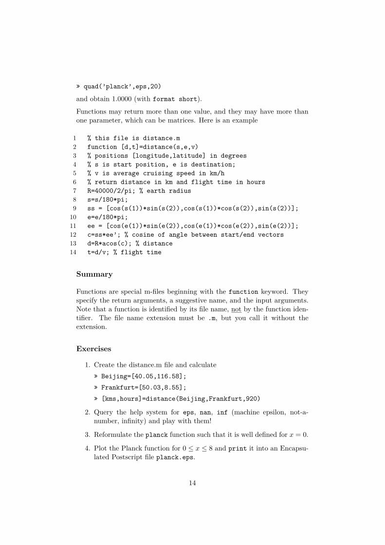
Functions may return more than one value, and they may have more thanone parameter, which can be matrices. Here is an example

1 % this file is distance.m2 function [d,t]=distance(s,e,v)3 % positions [longitude,latitude] in degrees4 % s is start position, e is destination;5 % v is average cruising speed in km/h6 % return distance in km and flight time in hours7 R=40000/2/pi; % earth radius8 s=s/180*pi;9 ss = [cos(s(1))*sin(s(2)),cos(s(1))*cos(s(2)),sin(s(2))];10 e=e/180*pi;11 ee = [cos(e(1))*sin(e(2)),cos(e(1))*cos(e(2)),sin(e(2))];12 c=ss*ee’; % cosine of angle between start/end vectors13 d=R*acos(c); % distance14 t=d/v; % flight time

Summary

Functions are special m-files beginning with the function keyword. Theyspecify the return arguments, a suggestive name, and the input arguments.Note that a function is identified by its file name, not by the function iden-tifier. The file name extension must be .m, but you call it without theextension.

Exercises

1. Create the distance.m file and calculate» Beijing=[40.05,116.58];

» Frankfurt=[50.03,8.55];

» [kms,hours]=distance(Beijing,Frankfurt,920)

2. Query the help system for eps, nan, inf (machine epsilon, not-a-number, infinity) and play with them!

3. Reformulate the planck function such that it is well defined for x = 0.

4. Plot the Planck function for 0 ≤ x ≤ 8 and print it into an Encapsu-lated Postscript file planck.eps.

14

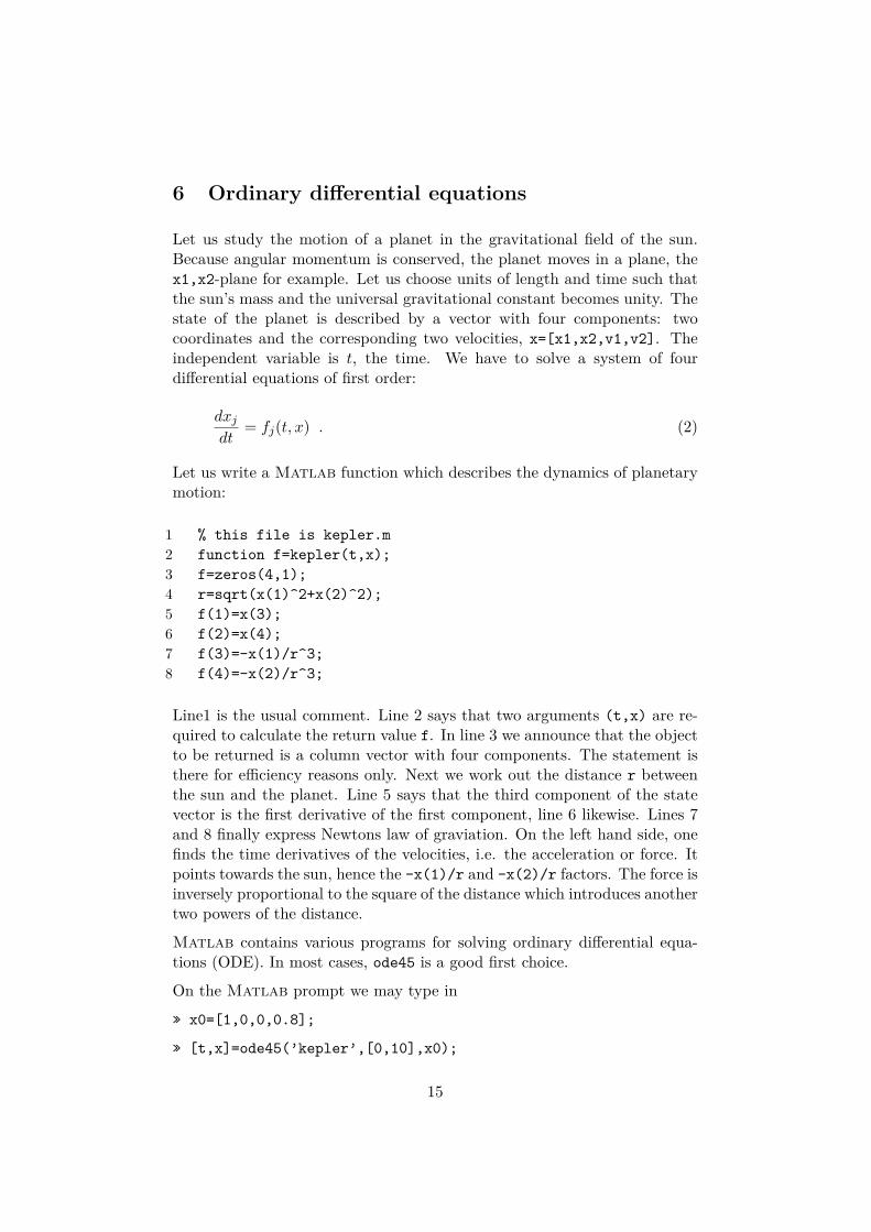
6 Ordinary differential equations

Let us study the motion of a planet in the gravitational field of the sun.Because angular momentum is conserved, the planet moves in a plane, thex1,x2-plane for example. Let us choose units of length and time such thatthe sun’s mass and the universal gravitational constant becomes unity. Thestate of the planet is described by a vector with four components: twocoordinates and the corresponding two velocities, x=[x1,x2,v1,v2]. Theindependent variable is t, the time. We have to solve a system of fourdifferential equations of first order:

dxj

dt= fj(t, x) . (2)

Let us write a Matlab function which describes the dynamics of planetarymotion:

1 % this file is kepler.m2 function f=kepler(t,x);3 f=zeros(4,1);4 r=sqrt(x(1)^2+x(2)^2);5 f(1)=x(3);6 f(2)=x(4);7 f(3)=-x(1)/r^3;8 f(4)=-x(2)/r^3;

Line1 is the usual comment. Line 2 says that two arguments (t,x) are re-quired to calculate the return value f. In line 3 we announce that the objectto be returned is a column vector with four components. The statement isthere for efficiency reasons only. Next we work out the distance r betweenthe sun and the planet. Line 5 says that the third component of the statevector is the first derivative of the first component, line 6 likewise. Lines 7and 8 finally express Newtons law of graviation. On the left hand side, onefinds the time derivatives of the velocities, i.e. the acceleration or force. Itpoints towards the sun, hence the -x(1)/r and -x(2)/r factors. The force isinversely proportional to the square of the distance which introduces anothertwo powers of the distance.

Matlab contains various programs for solving ordinary differential equa-tions (ODE). In most cases, ode45 is a good first choice.

On the Matlab prompt we may type in

» x0=[1,0,0,0.8];

» [t,x]=ode45(’kepler’,[0,10],x0);

15

x0 is the start vector. At t=0 our planet starts at (x1,x2)=(1,0) with ve-locity (v1,v2)=(0,0.8). This is the aphel, the position of largest distance.The next line calls ode45 with the minimum number of arguments: the dif-ferential equation to solve (an m-file), the time span, and the start vector.The function returns a vector t of time points and an array of correspondingpositions. The semicolon suppresses output to the command window.

Note that the returned x is a matrix. For each time in t, there is a rowvector in x, the corresponding state. This is an inconsistency (less politely:an error). The m-file requires the state to be a column vector, but the ODEsolver returns rows, one for each time.

We extract the first and second column which are the planet’s coordinates:

» x1=x(:,1);

» x2=x(:,2);

The colon operator : is short for "all components". If you now order

» plot(x1,x2)

you should see a few orbits. Because of inaccuracies they do not lie on oneand the same ellipse.

We insert before the ode45 command

» options=odeset(’RelTol’,1e-6);

and change the ode45 command into

» [t,x]=ode45(’kepler’,[0:0.05:10],x0,options);

These are two modifications. First, the time span has been detailed. Second,the relative integration tolerance is lowered. Now all orbits are one and thesame ellipse, in accordance with the findings of Kepler and Newton.

Summary

Integrating ordinary differential equations is a simple problem, in principle.First, you have to rewrite your problem into a system of coupled first-orderequations. Second, an m-file must be created which describes the drivativein terms of the independet variable and the state vector. Third, you startwith the standard ODE solver ode45. If you are not yet satisfied, refine thetime span and set options. If this does not resolve your problems, study theMatlab help system for alternative ODE solvers, or write one yourself.

16

Exercises

1. Implement the crude integration, as outlined above.

2. Work out from the returned set of states the angular momentuml=x(:,1).*x(:,4)-x(:,2).*x(:,3) and the total energy (likewise).

3. How constant are they? Do the same after the integration procedurehas been refined.

4. Study the options record returned by odeset.

5. Modify the kepler.m program in such a way that the force is inverseproportional to the first power of the distance, instead of the secondpower.

6. Create a random matrix a=rand(3,5) and study the effect of

• » a(:,1)

• » a(1,:)

• » a([1,2],[1,2])

• » a([1:3],:)

• » a(1,[1:2:5])

7. Write an essay ’Matlab: How to extract submatrices’ of not morethan two pages.

17

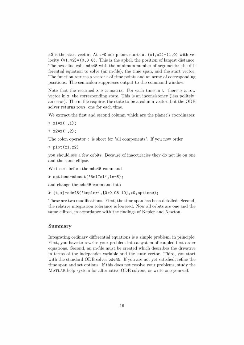
7 Reading and writing data

As we know, Matlab is concerned with matrices. s=’Matlab’ for in-stance, a string, is a 1 × 6 character array requiring 12 bytes of storage.r=[1,2;3,4;5,6], a 3 × 2 matrix of numbers, uses 48 bytes, c=r+i needs96 bytes.

There is a command who listing all currently active variables. Anothercommand, whos, adds size information.

A simple command like

» x=randn(2000)+i*randn(2000);

may consume a lot of memory, 64 MB in this case. If you do not need x anylonger, say

» clear x;

We recommend freeing memory whenever possible. Note that variableswhich are local to a function are destroyed automatically.

If you type

» save;

the entire workspace is saved to a disk file.

» clear all;

will clear the entire workspace. But it is not lost. Just type

» load;

Matlab knows which file to read and how to restore the original data.

You save a single matrix by

» save x;

A file x.mat is created which contains the data in binary form. We recom-mend

» save x.dat x -ascii -double;

The first argument is the file to be created, the second the matrix to besaved. The -ascii option provides for plain text, an additional -doubleavoids loss of precision. You may inspect this file with your favourite editor.

» load x.dat

opens the file, creates a matrix x of proper size and assigns to it the valuesstored in the file.

18

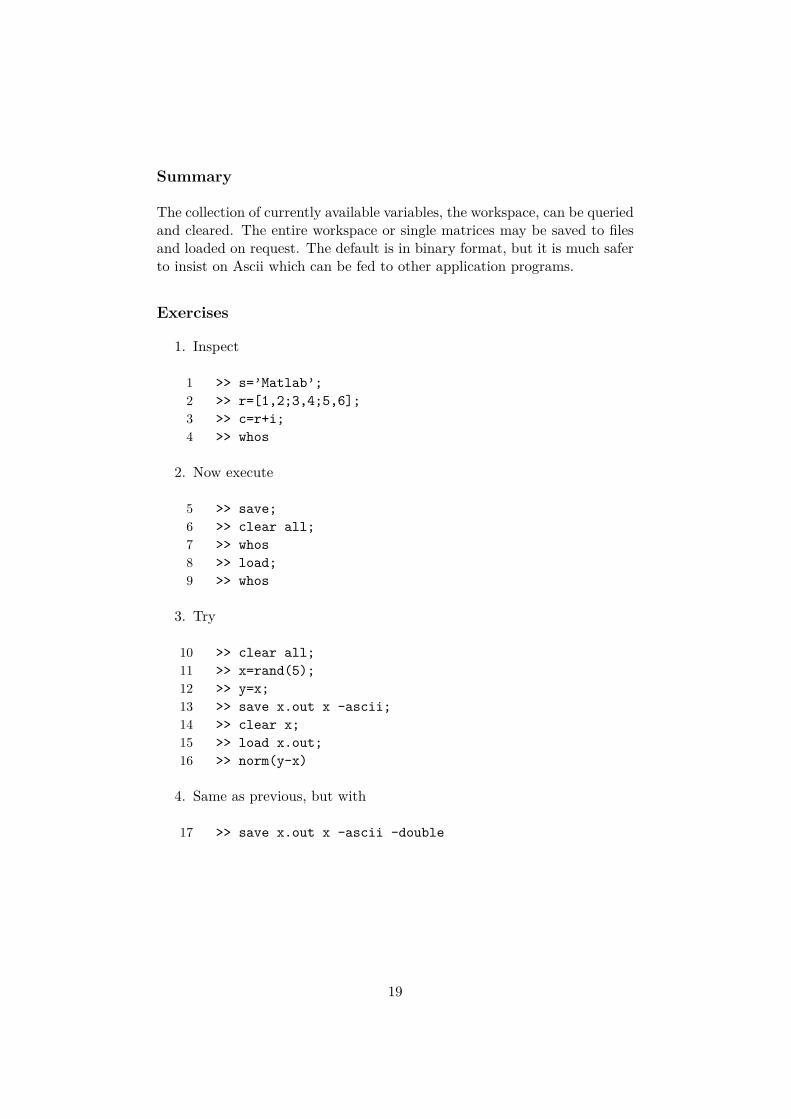
Summary

The collection of currently available variables, the workspace, can be queriedand cleared. The entire workspace or single matrices may be saved to filesand loaded on request. The default is in binary format, but it is much saferto insist on Ascii which can be fed to other application programs.

Exercises

1. Inspect

1 >> s=’Matlab’;2 >> r=[1,2;3,4;5,6];3 >> c=r+i;4 >> whos

2. Now execute

5 >> save;6 >> clear all;7 >> whos8 >> load;9 >> whos

3. Try

10 >> clear all;11 >> x=rand(5);12 >> y=x;13 >> save x.out x -ascii;14 >> clear x;15 >> load x.out;16 >> norm(y-x)

4. Same as previous, but with

17 >> save x.out x -ascii -double

19

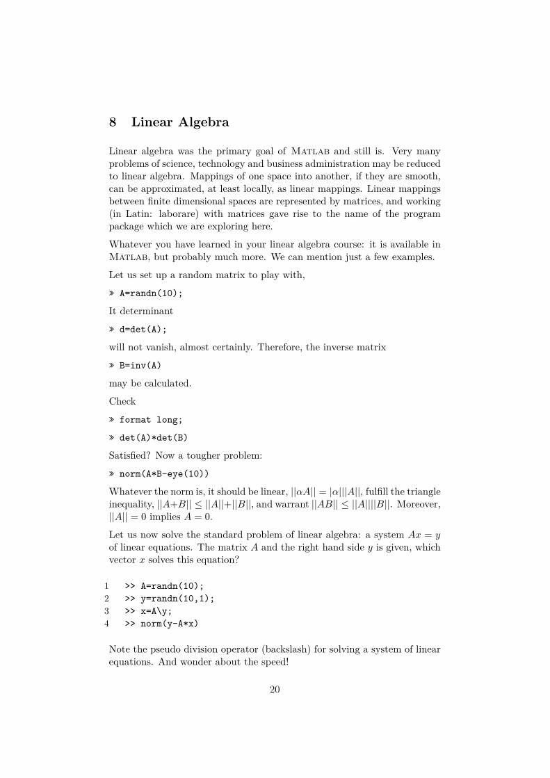
8 Linear Algebra

Linear algebra was the primary goal of Matlab and still is. Very manyproblems of science, technology and business administration may be reducedto linear algebra. Mappings of one space into another, if they are smooth,can be approximated, at least locally, as linear mappings. Linear mappingsbetween finite dimensional spaces are represented by matrices, and working(in Latin: laborare) with matrices gave rise to the name of the programpackage which we are exploring here.

Whatever you have learned in your linear algebra course: it is available inMatlab, but probably much more. We can mention just a few examples.

Let us set up a random matrix to play with,

» A=randn(10);

It determinant

» d=det(A);

will not vanish, almost certainly. Therefore, the inverse matrix

» B=inv(A)

may be calculated.

Check

» format long;

» det(A)*det(B)

Satisfied? Now a tougher problem:

» norm(A*B-eye(10))

Whatever the norm is, it should be linear, ||αA|| = |α|||A||, fulfill the triangleinequality, ||A+B|| ≤ ||A||+||B||, and warrant ||AB|| ≤ ||A||||B||. Moreover,||A|| = 0 implies A = 0.

Let us now solve the standard problem of linear algebra: a system Ax = yof linear equations. The matrix A and the right hand side y is given, whichvector x solves this equation?

1 >> A=randn(10);2 >> y=randn(10,1);3 >> x=A\y;4 >> norm(y-A*x)

Note the pseudo division operator (backslash) for solving a system of linearequations. And wonder about the speed!

20

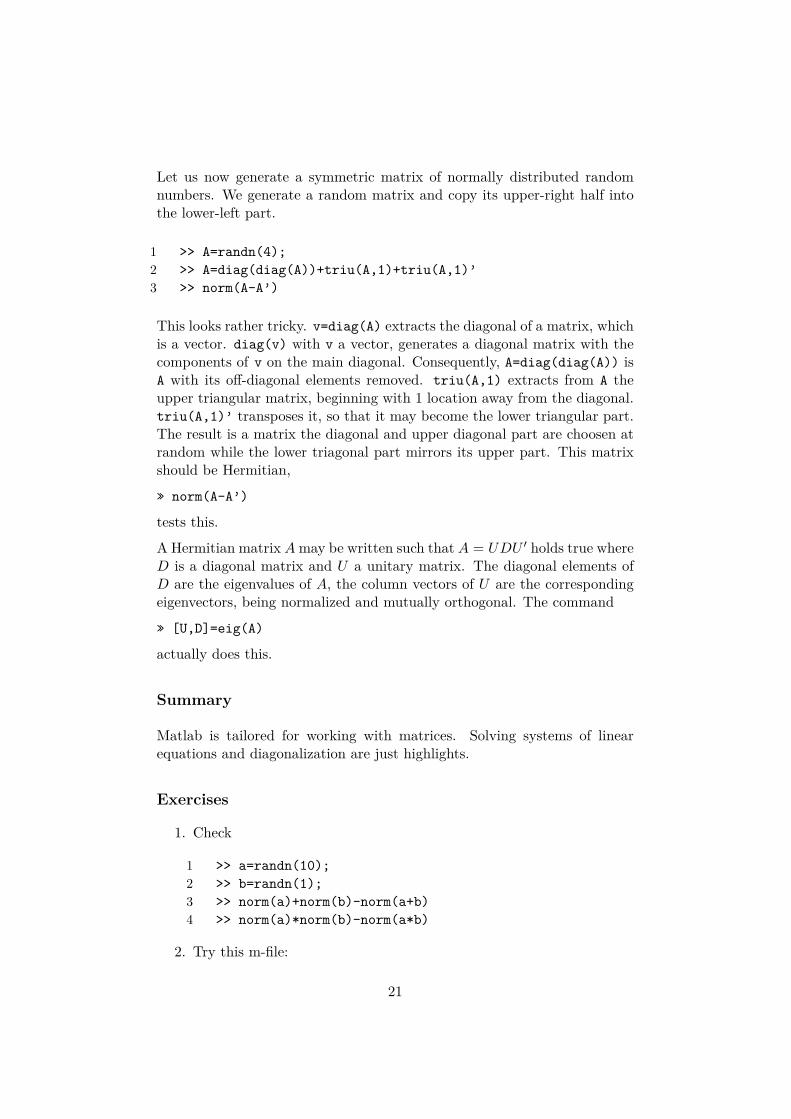
Let us now generate a symmetric matrix of normally distributed randomnumbers. We generate a random matrix and copy its upper-right half intothe lower-left part.

1 >> A=randn(4);2 >> A=diag(diag(A))+triu(A,1)+triu(A,1)’3 >> norm(A-A’)

This looks rather tricky. v=diag(A) extracts the diagonal of a matrix, whichis a vector. diag(v) with v a vector, generates a diagonal matrix with thecomponents of v on the main diagonal. Consequently, A=diag(diag(A)) isA with its off-diagonal elements removed. triu(A,1) extracts from A theupper triangular matrix, beginning with 1 location away from the diagonal.triu(A,1)’ transposes it, so that it may become the lower triangular part.The result is a matrix the diagonal and upper diagonal part are choosen atrandom while the lower triagonal part mirrors its upper part. This matrixshould be Hermitian,

» norm(A-A’)

tests this.

A Hermitian matrix Amay be written such that A = UDU ′ holds true whereD is a diagonal matrix and U a unitary matrix. The diagonal elements ofD are the eigenvalues of A, the column vectors of U are the correspondingeigenvectors, being normalized and mutually orthogonal. The command

» [U,D]=eig(A)

actually does this.

Summary

Matlab is tailored for working with matrices. Solving systems of linearequations and diagonalization are just highlights.

Exercises

1. Check

1 >> a=randn(10);2 >> b=randn(1);3 >> norm(a)+norm(b)-norm(a+b)4 >> norm(a)*norm(b)-norm(a*b)

2. Try this m-file:

21

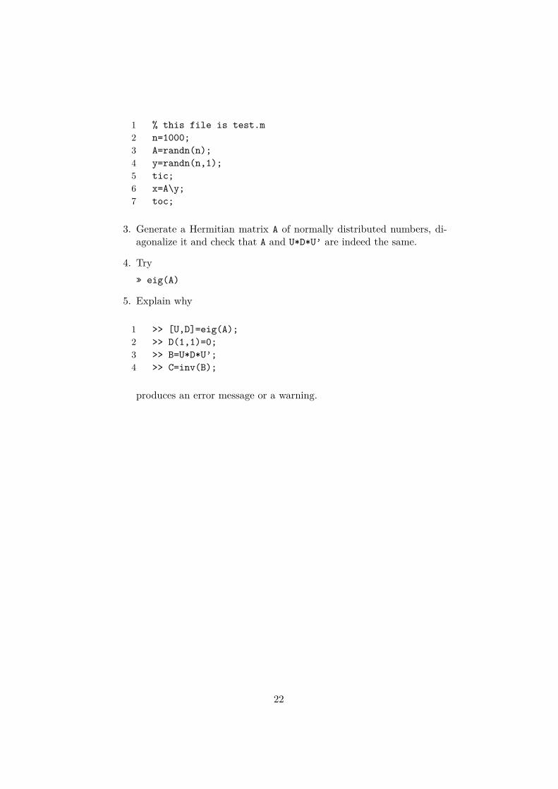
1 % this file is test.m2 n=1000;3 A=randn(n);4 y=randn(n,1);5 tic;6 x=A\y;7 toc;

3. Generate a Hermitian matrix A of normally distributed numbers, di-agonalize it and check that A and U*D*U’ are indeed the same.

4. Try» eig(A)

5. Explain why

1 >> [U,D]=eig(A);2 >> D(1,1)=0;3 >> B=U*D*U’;4 >> C=inv(B);

produces an error message or a warning.

22

9 Their logo

What is now their logo, was a challenge to programmers for a long time:solve the wave equation

∆u+ λu = 0 (3)

on an L-shaped domain Ω = [−1, 1]× [−1, 1]− [−1, 0)× [−1, 0).

u shall vanish on the boundary ∂Ω.

We approximate the x-axis by xj = jh with integer j and the y-axis byyk = hk with integer k. The field u at (xj , yk) is denoted by uj,k. Weapproximate ∆u at (xj , yk) by

(∆u)j,k = uj+1,k + uj,k+1 + uj−1,k + uj,k−1 − 4uj,k

h2 . (4)

Interior points of Ω—which are labelled by a = 1, 2, . . .—correspond to fieldvariables ua, and the Laplacien is represented by a matrix Lba. We look fora non-vanishing field ua such that

∑b Lbaub + λua = 0 holds, and λ shall be

the smallest value for which this is possible.

The following main program describes the domain Ω by a rectangular matrixD which assumes values 1 (interior point, variable) and 0 (field vanishes).A subprogram calculates the sparse Laplacien matrix L and the variablemapping: j = J(a) and k = K(a) yield the coordinates (xj , yk) for thevariable ua. We then look for one (1) eigenvalue (closest to 0.0) of thesparse matrix L by [u,d]=eigs(L,1,0.0); the field u and the eigenvalue dis returned. We then transform ua into uj,k = u(xj , yk). A graphical meshrepresentation is produced and saved into an encapsulated postscript file.

1 % this file is logo.m2 N=32; % resolution3 x=linspace(-1,1,N);4 y=linspace(-1,1,N);5 [X,Y]=meshgrid(x,y);6 D=(abs(X)<1)&(abs(Y)<1)&((X>0)|(Y>0));7 [L,J,K]=laplace(D);8 [u,d]=eigs(L,1,0.0);9 U=zeros(N,N);

10 for a=1:size(u)11 U(J(a),K(a))=u(a);12 end;13 mesh(U);14 print -depsc ’logo.eps’

23

The main program calls a function program Laplace:

1 % this file is laplace.m2 function [L,J,K]=laplace(D);3 [Nx,Ny]=size(D);4 jj=zeros(Nx*Ny,1);5 kk=zeros(Nx*Ny,1);6 aa=zeros(Nx,Ny);7 Nv=0;8 for j=1:Nx9 for k=1:Ny10 if D(j,k)==111 Nv=Nv+1;12 jj(Nv)=j;13 kk(Nv)=k;14 aa(j,k)=Nv;15 end;16 end;17 end;18 L=sparse(Nv,Nv);19 for a=1:Nv20 j=jj(a);21 k=kk(a);22 L(a,a)=-4;23 if D(j+1,k)==124 L(a,aa(j+1,k))=1;25 end;26 if D(j-1,k)==127 L(a,aa(j-1,k))=1;28 end;29 if D(j,k+1)==130 L(a,aa(j,k+1))=1;31 end;32 if D(j,k-1)==133 L(a,aa(j,k-1))=1;34 end;35 end;36 J=jj(1:Nv);37 K=kk(1:Nv);

The program is certainly suboptimal. It makes use of the for statementand resorts to if statements within loops. This can be repaired, althoughthe code will become less readable. Also note that a rather impressive 3Dgraphics has been produced by a command as simple as mesh(U).

24

05

1015

2025

3035

0

10

20

30

400

0.01

0.02

0.03

0.04

0.05

0.06

0.07

0.08

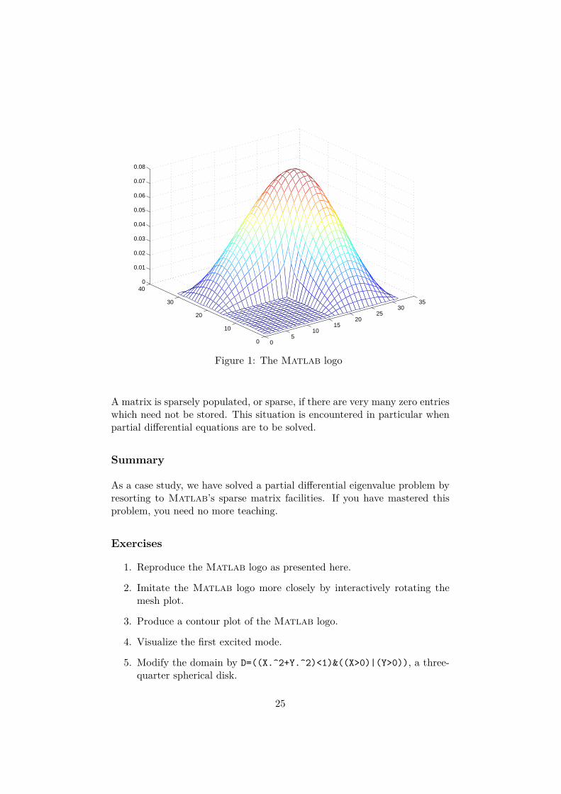
Figure 1: The Matlab logo

A matrix is sparsely populated, or sparse, if there are very many zero entrieswhich need not be stored. This situation is encountered in particular whenpartial differential equations are to be solved.

Summary

As a case study, we have solved a partial differential eigenvalue problem byresorting to Matlab’s sparse matrix facilities. If you have mastered thisproblem, you need no more teaching.

Exercises

1. Reproduce the Matlab logo as presented here.

2. Imitate the Matlab logo more closely by interactively rotating themesh plot.

3. Produce a contour plot of the Matlab logo.

4. Visualize the first excited mode.

5. Modify the domain by D=((X.^2+Y.^2)<1)&((X>0)|(Y>0)), a three-quarter spherical disk.

25