doing physics with matlab quantum physics …
TRANSCRIPT
1
DOING PHYSICS WITH MATLAB
QUANTUM PHYSICS
SCHRODINGER EQUATION
Solving the one-dimensional Schrodinger Equation for bound states in
a variety of potential wells using a matrix method that evaluates the
eigenvalues and eigenfunctions
Ian Cooper
School of Physics, University of Sydney
DOWNLOAD DIRECTORY FOR MATLAB SCRIPTS
The Matlab scripts are used to give the solution of the Schrodinger Equation for a variety
of potential energy functions using a matrix method where the solution are the
eigenvalues and eigenfunctions of the energy operator.
se_wells.m First m-script to be run when solving the Schrodinger Equation using the Matrix Method.
Most of the constants and all the well parameters are declared in this file. You can select
the type of potential well from the Command Window when the m-script is run. You
alter the m-script code to change the parameters that characterize the wells and you can
add to the m-script to define your own potential well. When this m-script is run it clears
all variables and closes all open Figure Windows.
se_solve.m This m-script solves the Schrodinger Equation using the Matrix Method after you have
run the m-script se_wells.m. The eigenvalues and corresponding eigenvectors are found
for the bound states of the selected potential well.
se_psi.m To be run after se_wells.m and se_solve.m. A graphical output displays the total energy,
the potential energy function, kinetic energy function, eigenvector and probability
distribution for a given quantum state.
2
se_measurements.m To be run after se_wells.m and se_solve.m. Evaluates the expectation values for a set of
dynamic quantities: the inherent quantum-mechanical uncertainties in measurements and
gives a test of the Heisenberg uncertainty principle.
se_orthonormal.m To be run after se_wells.m and se_solve.m. You can investigate the orthonormal
characteristic of the eigenvectors (stationary state wavefunctions).
se_infwell.m Used to test the accuracy of the Matrix Method. Compares the analytical and numerical
results for an infinite square well potential of width 0.1 nm.
simpson1d.m Function to evaluate the area under a curve using Simpson’s 1/3 rule.
Colorcode.m Function to return the appropriate colour for a wavelength in the visible range from 380
nm to 780 nm.
gaussian_p.m Produces a graphical display of a Gaussian shaped potential well and the corresponding
force graph.
Using the m-script to solve the Schrodinger Equation
Run se_wells.m then se_solve.m
Then any of the following can be run to investigate the solution:
se_orthonormal.m (orthonormal characteristic of wavefunctions)
se_psi.m (displays energy functions and wavefunctions)
se_measurements.m (calculation of expectation values)

3
SCHRODINGER EQUATION
On an atomic scale, all particles exhibit a wavelike behavior. Particles can be represented
by wavefunctions which obey a differential equation, the Schrodinger Wave Equation
which relates spatial coordinates and time. You can gain valuable insight into quantum
mechanics by studying the solutions to the one-dimensional time independent
Schrodinger Equation.
A wave equation that describes the behavior of an electron was developed by Schrodinger
in 1925. He introduced a wavefunction ( , , , )x y z t . This is a purely mathematical
function and does not represent any physical entity. An interpretation of the wave
function was given by Born in 1926 who suggested that the quantity 2
( , , , )x y z t
represents the probability density of finding an electron. For the one dimensional case,
the probability of finding the electron at time t somewhere between x1 and x2 is given by
(1) 2
1
*Prob( ) ( , ) ( , )x
xt x t x t dx
where * is the complex conjugate of the wavefunction . The value of Prob(t) must lie
between 0 and 1 and so when we integrate over all space, the probability of finding the
electron must be 1.
*( , ) ( , ) 1x t x t dx
In this instance the wavefunction is said to be normalized.
We can see how the time-independent Schrodinger Equation in one dimension is
plausible for a particle of mass m, whose motion is governed by a potential energy
function U(x) by starting with the classical one dimensional wave equation and using the
de Broglie relationship
Classical wave equation 2 2
2 2 2
( , ) 1 ( , )0
x t x t
x v t
Momentum (de Broglie) h
p mv k
4
Kinetic energy 212
K mv
Total energy ( ) ( )E K x U x
Wavefunction ( , ) ( ) i tx t x e periodic in time for t coordinate
Combining the above relationships, the time-independent Schrodinger Equation in one
dimension can be expressed as
(2) 2 2
2
( )( ) ( ) ( )
2
d xU x x E x
m dx
Our goal is to find solutions of this form of the Schrodinger Equation for a potential
energy function which traps the particle within a region. The negative slope of the
potential energy function gives the force on the particle. For the particle to be bound the
force acting on the particle is attractive. The solutions must also satisfy the boundary
conditions for the wavefunction. The probability of finding the particle must be 1,
therefore, the wavefunction must approach zero as the position from the trapped region
increases. The imposition of the boundary conditions on the wavefunction results in a
discrete set of values for the total energy E of the particle and a corresponding
wavefunction for that energy, just like a vibrating guitar string which has a set of normal
modes of vibration in which there is a harmonic sequence for the vibration frequencies.
The Schrodinger Equation can be solved analytically for only a few forms of the potential
energy function. In this paper, we will consider a numerical approach to solving the
Schrodinger Equation using a matrix method where the eigenvalues of a matrix gives
the total energies of the particle and the eigenfunctions the corresponding wavefunctions.
5
MATRIX METHOD
The one-dimensional time independent Schrodinger Equation can be expressed as
(3)
2
2
2 2
2 2
( )( ) ( ) ( )
2
( ) ( ) ( )2
( ) ( )
d xU x x E x
m dx
dU x x E x
m dx
H x E x
where the H is the Hamiltonian operator, which is the operator that corresponds to the
total energy of the system. This is an eigenvalue equation. The action of the operator H
on the function returns the original function multiplied by a constant which could be
complex. This eigenvalue equation is generally satisfied by a particular set of functions
1 2( ), ( ), ,x x and a corresponding set of constants 1 2, ,E E . These are the
eigenfunctions and the corresponding eigenvalues of the operator H. The time
independent Schrodinger Equation of a system is the energy eigenvalue equation of the
system. An eigenfunction ( )n x describes a state of define energy En. When the energy
of the system in this state is measured, the result will always be En. For the eigenfunction
to represent physical sensible solutions, we require
( ) 0 asn x x
so that the wavefunction can be normalized.
For atomic systems it is more convenient to measure lengths in nm (nanometers) and
energies in eV (electron volts). We can use the scaling factors
length: Lse = 1×10⁻⁹
to convert m into nm
energy: Ese = 1.6×10⁻¹⁹
to convert J into eV
and so we can write equation (5) as
(4)
2
2
2 2
2
2 2
2
1( ) ( ) ( )
2
1( ) ( ) ( ) where
2
( ) ( )
se se
se se
se se
dU x x E x
m L E dx
dC U x x E x C
dx m L E
H x E x
6
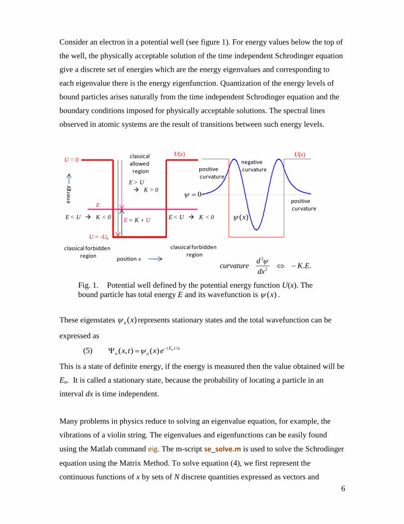
Consider an electron in a potential well (see figure 1). For energy values below the top of
the well, the physically acceptable solution of the time independent Schrodinger equation
give a discrete set of energies which are the energy eigenvalues and corresponding to
each eigenvalue there is the energy eigenfunction. Quantization of the energy levels of
bound particles arises naturally from the time independent Schrodinger equation and the
boundary conditions imposed for physically acceptable solutions. The spectral lines
observed in atomic systems are the result of transitions between such energy levels.
Fig. 1. Potential well defined by the potential energy function U(x). The
bound particle has total energy E and its wavefunction is ( )x .
These eigenstates ( )n x represents stationary states and the total wavefunction can be
expressed as
(5) /( , ) ( ) ni E t
n nx t x e
This is a state of definite energy, if the energy is measured then the value obtained will be
En. It is called a stationary state, because the probability of locating a particle in an
interval dx is time independent.
Many problems in physics reduce to solving an eigenvalue equation, for example, the
vibrations of a violin string. The eigenvalues and eigenfunctions can be easily found
using the Matlab command eig. The m-script se_solve.m is used to solve the Schrodinger
equation using the Matrix Method. To solve equation (4), we first represent the
continuous functions of x by sets of N discrete quantities expressed as vectors and
en
erg
y
position x
U(x)U = 0
E
U = -U0
E = K + UE < U K < 0 E < U K < 0
E > U
K > 0
classical forbiddenregion
classical forbiddenregion
classicalallowed
region
2
2. .
dcurvature K E
dx
( )x
0 positivecurvature
positivecurvature
negativecurvature
U(x)
7
matrices. The discrete set of x values is represented by the vector nx the corresponding
wavefunctions by the vector n . The potential energy is given by a (N-2)(N-2)
diagonal matrix [U] with diagonal element Un. A sample code [se_solve.m] for assigning
the diagonal elements for [U] is
… U_matrix = zeros(N-2,N-2);
… for c = 1 : N-2
U_matrix (c,c) = U(c); end
Next, we have to represent the operator
2
2 2
2
d
m dx
as a matrix of size (N-2)(N-2). From the definitions of the first and second derivatives of
the function y(x), we can approximate them by the equations
1/ 2
1
n
n n
x
dy y y
dx x
1/ 2 1/ 2
2
1 1
2 2
1 2
n nn
n n n
x xx
d y dy dy y y y
dx x dx dx x
Hence, the second derivative matrix for N = 6 can be written as a 44 matrix
2
2 1 0 0
1 2 1 01[ ]
0 1 2 1
0 0 1 2
x
SD
The SD matrix size is (N-2)(N-2) and not NN because the second derivative of the
function can’t be evaluated at the end points, n = 1 and n = N. The kinetic energy matrix
[K] is then defined as
[ ] seCK SD
We can now define the Hamiltonian matrix as
[ ] H K U
8
A sample code [se_solve.m] for the generating the Hamiltonian matrix is
% Make Second Derivative Matrix ------------------------------------------ off = ones(num-3,1); SD_matrix = (-2*eye(num-2) + diag(off,1) + diag(off,-1))/dx2;
% Make KE Matrix K_matrix = Cse * SD_matrix;
% Make Hamiltonian Matrix H_matrix = K_matrix + U_matrix;
Therefore, the Schrodinger Equation in matrix form is
(6) [ ] n n nE H
This is an eigenvalue equation in matrix form where the action of the Hamilton matrix
results in each value to be the vector n being multiplied by a multiplied by the set of
numbers En. The set of numbers En are called the eigenvalues and set of vectors n are
the eigenvectors.
This is a single Matlab function that finds both the eigenvalues and eigenvectors. The
syntax of the command is
[e_funct, e_values] = eig(H)
where e_funct is an (N-2)(N-2) matrix with the nth
column corresponding to the nth
eigenfunction and e_values is a column vector for the N eigenvalues in increasing order.
Only the negative values of e_values are significant. To obtain the complete eigenvector
we need to include the end points where min max( ) ( ) 0n nx x . A sample Malab code
[se_solve.m] to obtain the discrete set of eigenvalues and normalized eigenfunction is
9
% All Eigenvalues 1, 2 , ... n where E_N < 0 flag = 0; n = 1; while flag == 0 E(n) = e_values(n,n); if E(n) > 0, flag = 1; end; % if n = n + 1; end % while E(n-1) = []; n = n-2; % Corresponding Eigenfunctions 1, 2, ... ,n: Normalizing the wavefunction for cn = 1 : n psi(:,cn) = [0; e_funct(:,cn); 0]; area = simpson1d((psi(:,cn) .* psi(:,cn))',xMin,xMax); psi(:,cn) = psi(:,cn)/sqrt(area); prob(:,cn) = psi(:,cn) .* psi(:,cn); end % for
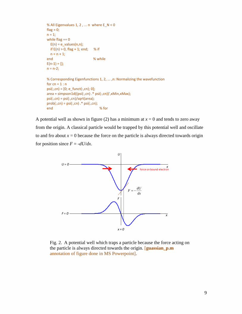
A potential well as shown in figure (2) has a minimum at x = 0 and tends to zero away
from the origin. A classical particle would be trapped by this potential well and oscillate
to and fro about x = 0 because the force on the particle is always directed towards origin
for position since F = -dU/dx.
Fig. 2. A potential well which traps a particle because the force acting on
the particle is always directed towards the origin. [guassian_p.m
annotation of figure done in MS Powerpoint].
x
x
U
U = 0
F = 0
x = 0
F
force on bound electron
dUF
dx

10
We can solve the Schrodinger Equation (equation 6) for a variety of different potential
energy functions. The m-script SE_wells.m defines most of the constants and potential
well parameters. Within the m-script you can change the code to modify the potential
wells and add new potential wells. The first step in solving the Schrodinger Equation
using the Matrix Method for a bound electron is to run the file SE_wells.m and select the
type of potential well. The default potentials include:
1 Square well
2 Stepped well
3 Double well
4 Sloping well
5 Truncated Parabolic well
6 Morse Potential well
7 Parabolic fit to Morse Potential
8 Lattice
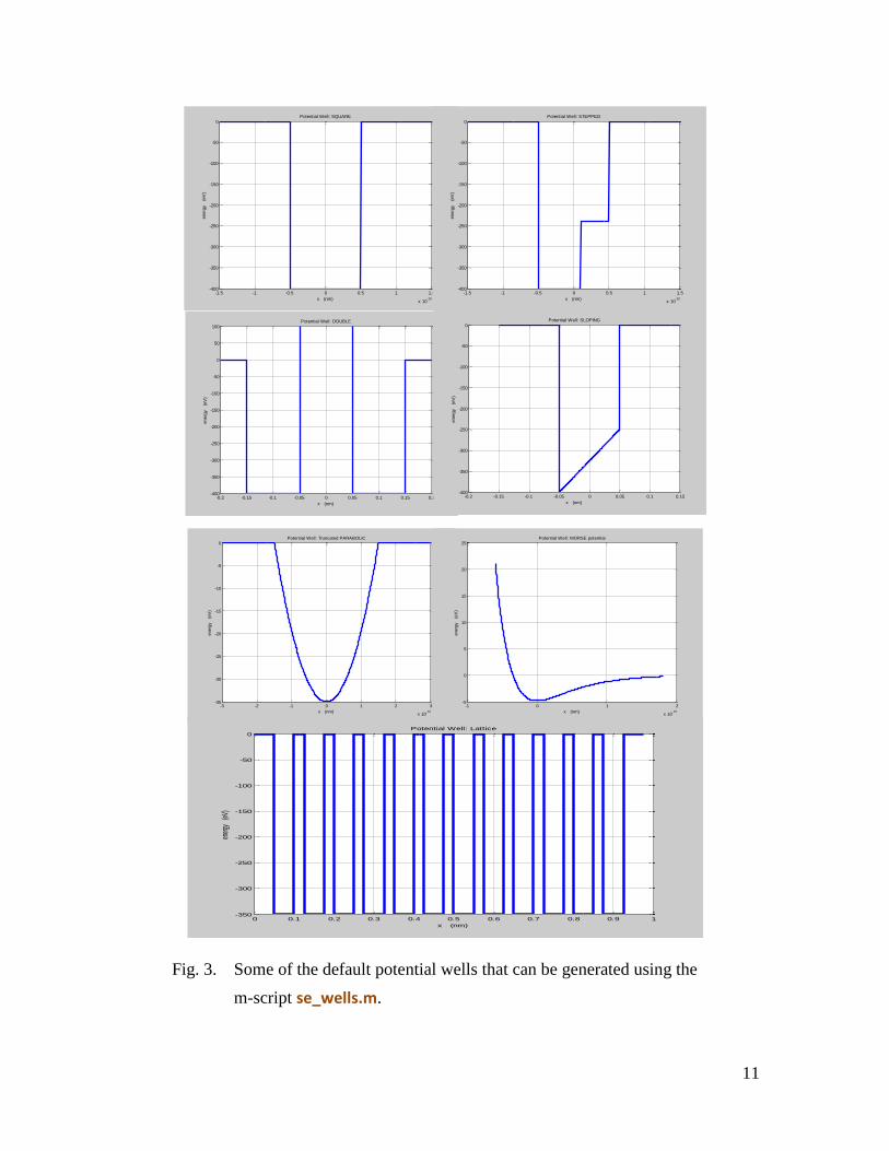
11
Fig. 3. Some of the default potential wells that can be generated using the
m-script se_wells.m.
-1.5 -1 -0.5 0 0.5 1 1.5
x 10-10
-400
-350
-300
-250
-200
-150
-100
-50
0Potential Well: SQUARE
x (nm)
energ
y
(eV
)
-1.5 -1 -0.5 0 0.5 1 1.5
x 10-10
-400
-350
-300
-250
-200
-150
-100
-50
0Potential Well: STEPPED
x (nm)
energ
y
(eV
)
-0.2 -0.15 -0.1 -0.05 0 0.05 0.1 0.15 0.2-400
-350
-300
-250
-200
-150
-100
-50
0
50
100Potential Well: DOUBLE
x (nm)
energ
y
(eV
)
-0.2 -0.15 -0.1 -0.05 0 0.05 0.1 0.15-400
-350
-300
-250
-200
-150
-100
-50
0Potential Well: SLOPING
x (nm)
energ
y
(eV
)
-3 -2 -1 0 1 2 3
x 10-10
-35
-30
-25
-20
-15
-10
-5
0Potential Well: Truncated PARABOLIC
x (nm)
energ
y
(eV
)
-1 0 1 2
x 10-10
-5
0
5
10
15
20
25Potential Well: MORSE potential
x (nm)
energ
y
(eV
)
0 0.1 0.2 0.3 0.4 0.5 0.6 0.7 0.8 0.9 1-350
-300
-250
-200
-150
-100
-50
0Potential Well: Lattice
x (nm)
ener
gy
(eV)
12
If you are not satisfied with the potential well that is displayed, you can change any of the
parameters in the m-script se_wells.m and run it again. Then to solve the Schrodinger
Equation run the m-script se_solve.m.
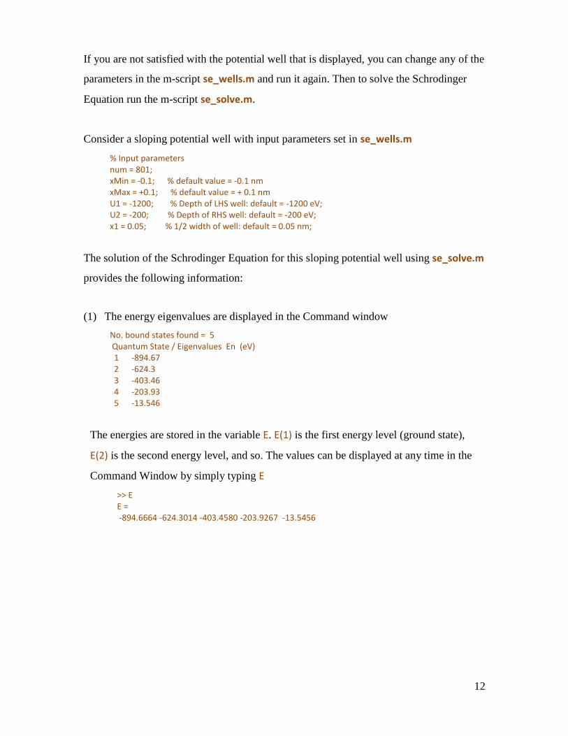
Consider a sloping potential well with input parameters set in se_wells.m
% Input parameters num = 801; xMin = -0.1; % default value = -0.1 nm xMax = +0.1; % default value = + 0.1 nm U1 = -1200; % Depth of LHS well: default = -1200 eV; U2 = -200; % Depth of RHS well: default = -200 eV; x1 = 0.05; % 1/2 width of well: default = 0.05 nm;
The solution of the Schrodinger Equation for this sloping potential well using se_solve.m
provides the following information:
(1) The energy eigenvalues are displayed in the Command window
No. bound states found = 5 Quantum State / Eigenvalues En (eV) 1 -894.67 2 -624.3 3 -403.46 4 -203.93 5 -13.546
The energies are stored in the variable E. E(1) is the first energy level (ground state),
E(2) is the second energy level, and so. The values can be displayed at any time in the
Command Window by simply typing E
>> E E = -894.6664 -624.3014 -403.4580 -203.9267 -13.5456
13
(2) A graph of the energy spectrum is shown in figure (4) for a sloping potential well
Fig. 4. The energy spectrum for a potential well produced by the m-script
se_solve.m.
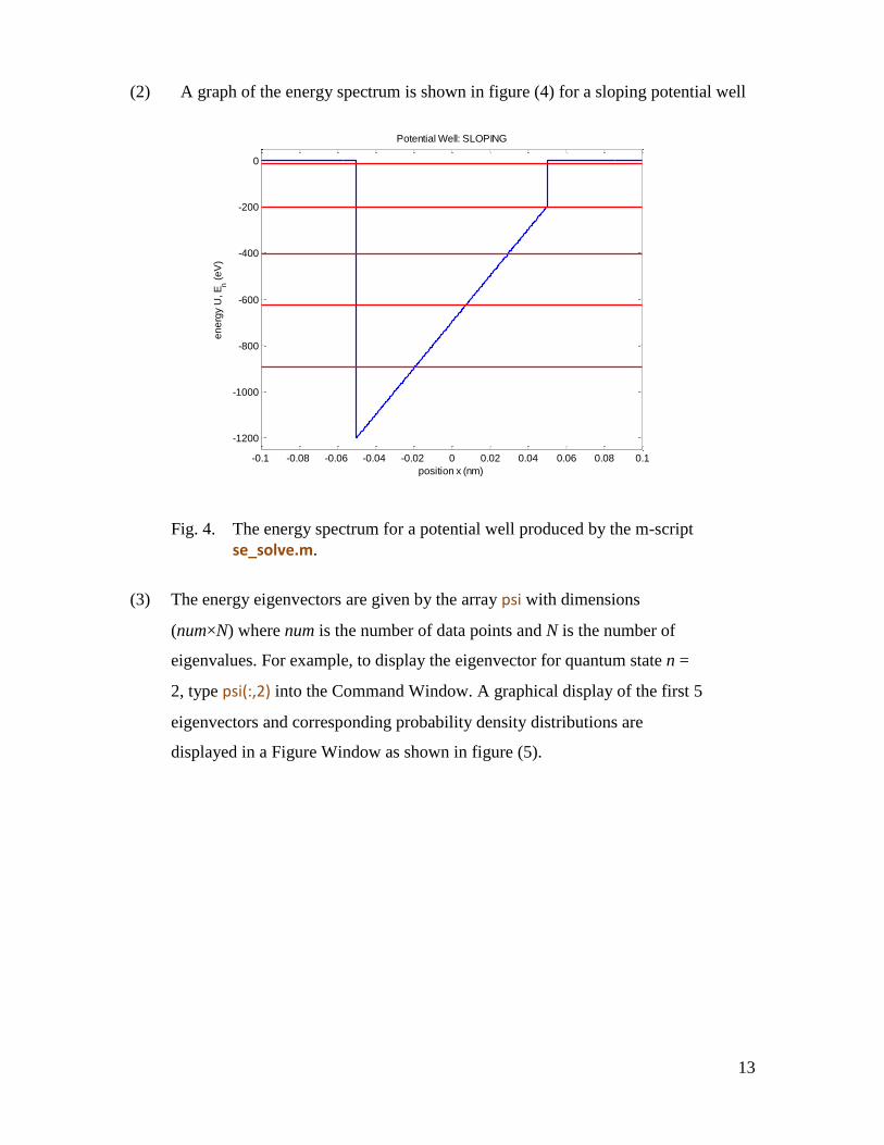
(3) The energy eigenvectors are given by the array psi with dimensions
(num×N) where num is the number of data points and N is the number of
eigenvalues. For example, to display the eigenvector for quantum state n =
2, type psi(:,2) into the Command Window. A graphical display of the first 5
eigenvectors and corresponding probability density distributions are
displayed in a Figure Window as shown in figure (5).
-0.1 -0.08 -0.06 -0.04 -0.02 0 0.02 0.04 0.06 0.08 0.1
-1200
-1000
-800
-600
-400
-200
0
position x (nm)
en
erg
y U
, E
n (
eV
)
Potential Well: SLOPING
14
Fig. 5. The energy eigenvectors and probability distributions for sloping
potential well. [se_solve.m].
To view a graphical display of an eigenvector and the probability density graphs for a
given state, you can run the m-script se_psi.m from the Command Window. The
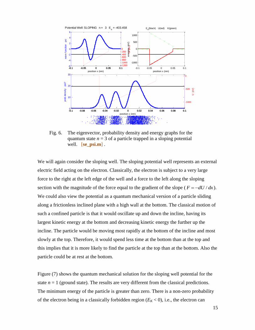
graphical output for a sloping potential well for quantum state n = 3 is shown in figure
(6). Variations with position of the eigenvector ( )n x ; probability density 2
( )n x ;
energies U(x), K(x), E are shown along with a probability cloud where each point
displayed shows the position of the particle after a measurement is made on the system
resulting in the collapse of the wavefunction.
n = 1 2 n = 1
n = 2 2 n = 2
n = 3 2 n = 3
n = 4 2 n = 4
n = 5 2 n = 5
15
Fig. 6. The eigenvector, probability density and energy graphs for the
quantum state n = 3 of a particle trapped in a sloping potential
well. [se_psi.m] .
We will again consider the sloping well. The sloping potential well represents an external
electric field acting on the electron. Classically, the electron is subject to a very large
force to the right at the left edge of the well and a force to the left along the sloping
section with the magnitude of the force equal to the gradient of the slope ( /F dU dx ).
We could also view the potential as a quantum mechanical version of a particle sliding
along a frictionless inclined plane with a high wall at the bottom. The classical motion of
such a confined particle is that it would oscillate up and down the incline, having its
largest kinetic energy at the bottom and decreasing kinetic energy the further up the
incline. The particle would be moving most rapidly at the bottom of the incline and most
slowly at the top. Therefore, it would spend less time at the bottom than at the top and
this implies that it is more likely to find the particle at the top than at the bottom. Also the
particle could be at rest at the bottom.
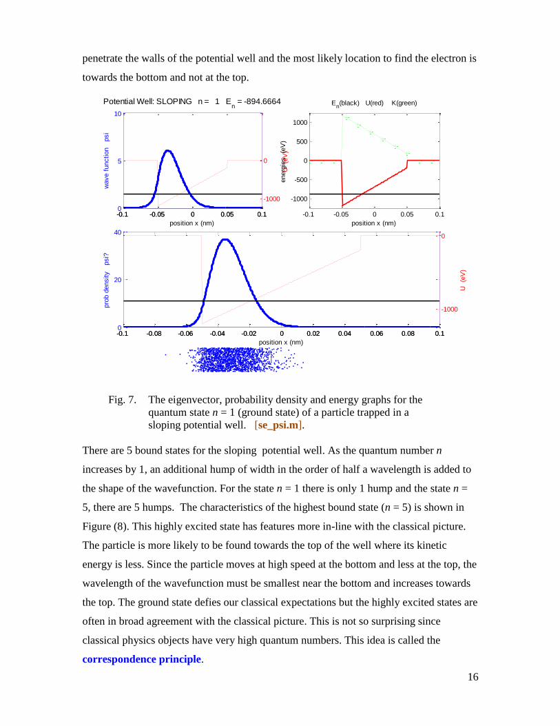
Figure (7) shows the quantum mechanical solution for the sloping well potential for the
state n = 1 (ground state). The results are very different from the classical predictions.
The minimum energy of the particle is greater than zero. There is a non-zero probability
of the electron being in a classically forbidden region (EK < 0), i.e., the electron can
-0.1 -0.05 0 0.05 0.1-6
-4
-2
0
2
4
6
Potential Well: SLOPING n = 3 En = -403.458
position x (nm)
wave f
unction
psi
-0.1 -0.05 0 0.05 0.1-1200-1000-800-600-400-2000
U
(eV
)
-0.1 -0.08 -0.06 -0.04 -0.02 0 0.02 0.04 0.06 0.08 0.10
10
20
30
position x (nm)
pro
b d
ensity
psi?
-0.1 -0.08 -0.06 -0.04 -0.02 0 0.02 0.04 0.06 0.08 0.1
-1000
-500
0
U
(eV
)
-0.1 -0.05 0 0.05 0.1
-1000
-500
0
500
1000
En(black) U(red) K(green)
position x (nm)
energ
ies
(eV
)
16
penetrate the walls of the potential well and the most likely location to find the electron is
towards the bottom and not at the top.
Fig. 7. The eigenvector, probability density and energy graphs for the
quantum state n = 1 (ground state) of a particle trapped in a
sloping potential well. [se_psi.m].
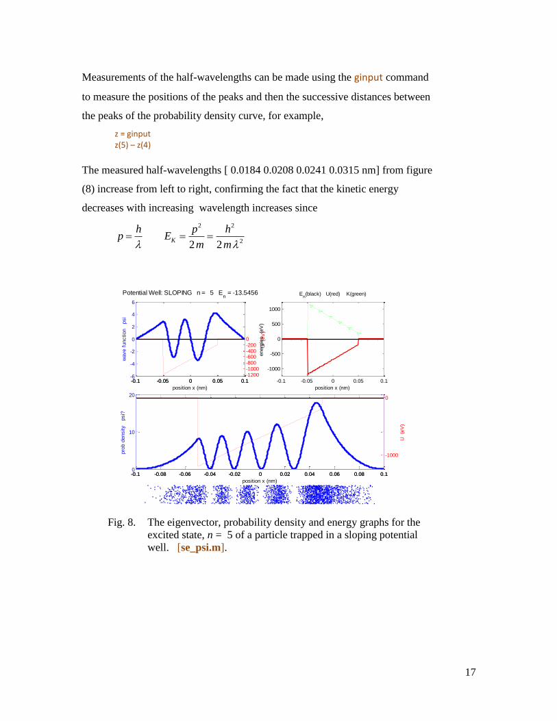
There are 5 bound states for the sloping potential well. As the quantum number n
increases by 1, an additional hump of width in the order of half a wavelength is added to
the shape of the wavefunction. For the state n = 1 there is only 1 hump and the state n =
5, there are 5 humps. The characteristics of the highest bound state (n = 5) is shown in
Figure (8). This highly excited state has features more in-line with the classical picture.
The particle is more likely to be found towards the top of the well where its kinetic
energy is less. Since the particle moves at high speed at the bottom and less at the top, the
wavelength of the wavefunction must be smallest near the bottom and increases towards
the top. The ground state defies our classical expectations but the highly excited states are
often in broad agreement with the classical picture. This is not so surprising since
classical physics objects have very high quantum numbers. This idea is called the
correspondence principle.
-0.1 -0.05 0 0.05 0.10
5
10
Potential Well: SLOPING n = 1 En = -894.6664
position x (nm)
wave f
unction
psi
-0.1 -0.05 0 0.05 0.1
-1000
0
U
(eV
)
-0.1 -0.08 -0.06 -0.04 -0.02 0 0.02 0.04 0.06 0.08 0.10
20
40
position x (nm)
pro
b d
ensity
psi?
-0.1 -0.08 -0.06 -0.04 -0.02 0 0.02 0.04 0.06 0.08 0.1
-1000
0
U
(eV
)
-0.1 -0.05 0 0.05 0.1
-1000
-500
0
500
1000
En(black) U(red) K(green)
position x (nm)
energ
ies
(eV
)
17
Measurements of the half-wavelengths can be made using the ginput command
to measure the positions of the peaks and then the successive distances between
the peaks of the probability density curve, for example,
z = ginput z(5) – z(4)
The measured half-wavelengths [ 0.0184 0.0208 0.0241 0.0315 nm] from figure
(8) increase from left to right, confirming the fact that the kinetic energy
decreases with increasing wavelength increases since
2 2
22 2K
h p hp E
m m
Fig. 8. The eigenvector, probability density and energy graphs for the
excited state, n = 5 of a particle trapped in a sloping potential
well. [se_psi.m].
-0.1 -0.05 0 0.05 0.1-6
-4
-2
0
2
4
6
Potential Well: SLOPING n = 5 En = -13.5456
position x (nm)
wave f
unction
psi
-0.1 -0.05 0 0.05 0.1-1200-1000-800-600-400-2000
U
(eV
)
-0.1 -0.08 -0.06 -0.04 -0.02 0 0.02 0.04 0.06 0.08 0.10
10
20
position x (nm)
pro
b d
ensity
psi?
-0.1 -0.08 -0.06 -0.04 -0.02 0 0.02 0.04 0.06 0.08 0.1
-1000
0U
(e
V)
-0.1 -0.05 0 0.05 0.1
-1000
-500
0
500
1000
En(black) U(red) K(green)
position x (nm)
energ
ies
(eV
)
18
EXPECTATION VALUES
The quantum behavior of bound particles is becoming more important in electronic
devices made using semiconductor materials such as silicon and gallium. The heart of
such devices is a tiny structure called a quantum dot that consists of a speck of one
semiconductor material (width ~ 1 nm, ~100’s atoms) completely enclosed by a much
larger semiconductor material. Some of the electrons in the tiny speck become detached
from their parent atoms and behave as particles trapped in potential wells of 1 dimension
(quantum wafer), 2 dimensions (quantum wire), or 3 dimensions (quantum dot). These
particles are often referred to as particles in a box. The bound electrons have a discrete
energy spectrum just like electrons bound in atoms. Quantum dots are often referred to as
artificial atoms. The light emitting properties of quantum dots are used in solid state
lasers such as DVD players, lighting systems, solar cells, fluorescent markers in
biomedical applications. Our focus of finding the physically acceptable solutions of the
Schrodinger Equation for bound particles is important to understanding real systems of
increasing technological importance.
The wavefunction that describes a quantum state provides the most complete description
that is possible of that state – it contains all the information we can possibly know about
this quantum state. But the wavefunction is not something that can be measured and
therefore has no physical meaning. The information we can get from the wavefunction is
related only to the probabilities of the possible outcomes of measurements made on
identical systems. Hence, there is an intrinsic and unavoidable indeterminism in the
quantum world.
When a measurement is made on a quantum system, the wavefunction collapses, the
state of the system after the measurement is not the same as the state before the
measurement. The Schrodinger Equation does not describe this collapse of the
wavefunction. So, for experiments designed to test the predictions of quantum mechanics,
you can’t do a sequence of measurements on a single system, rather, you start with a
large number of identical systems all in the same state and then perform the same
measurement of each system. Although each system is initially identical, the outcomes of
19
the measurements typically give a spread of results, for example, the measurement of the
position of the electron in passing through an equivalent of a double slit.
We will consider systems of a single electrons confined by a one dimensional potential
wells. We already know that it is a simple matter to use the wavefunction to find the
probability distribution for the position of the electron. However, we can extend this
method to find the probability distributions of other measureable quantities such as
position, momentum and energy. This information is contained in the shape of the
wavefunction and we will show how this information can be extracted.
For the electron trapped in the sloping potential wells the solution of the Schrodinger
Equation gave a set of energy eigenvalues and their corresponding eigenvectors
(stationary states). The energy eigenvalues are the only allowed energies of the system.
No matter what state the system is in, if we measure its energy, we always get one of the
energy eigenvalues. These stationary states are special, because they are states of definite
energy. So in this case, there is zero uncertainty in the measurements. If the system is
described by a stationary state wavefunction ( , )n x t and we measure its energy, we will
certainty get the result En for the energy eigenvalue.
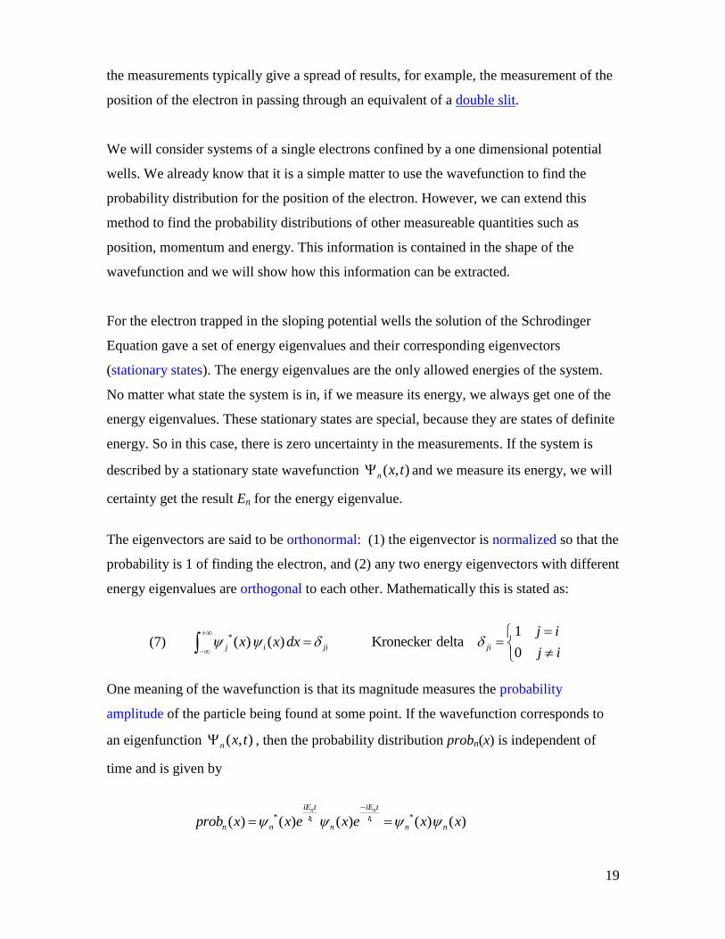
The eigenvectors are said to be orthonormal: (1) the eigenvector is normalized so that the
probability is 1 of finding the electron, and (2) any two energy eigenvectors with different
energy eigenvalues are orthogonal to each other. Mathematically this is stated as:
(7) *
1( ) ( ) Kronecker delta
0j i ji ji
j ix x dx
j i
One meaning of the wavefunction is that its magnitude measures the probability
amplitude of the particle being found at some point. If the wavefunction corresponds to
an eigenfunction ( , )n x t , then the probability distribution probn(x) is independent of
time and is given by
* *( ) ( ) ( ) ( ) ( )
n niE t iE t
n n n n nprob x x e x e x x
20
and the probability Pn of finding the particle between x1 and x2 is
2
1
*( ) ( )x
n n nx
P x x dx
We can also calculate probability distributions for other observable quantities in a similar
manner to above. The probability distribution is characterized by two measures – its
expectation value (estimate of the mean value of the distribution) and its uncertainty
(spread of values around the mean). Suppose that an observable quantity A has a discrete
set of possible values a1, a2, … . Then, we can prepare N identical systems, all in the
same state and measure the value of A in each system. In general, we will get a spread of
results. The best estimate of the quantity A is its mean value <A> and the standard
deviation A can be used as a measure of the spread or uncertainty in the measurements.
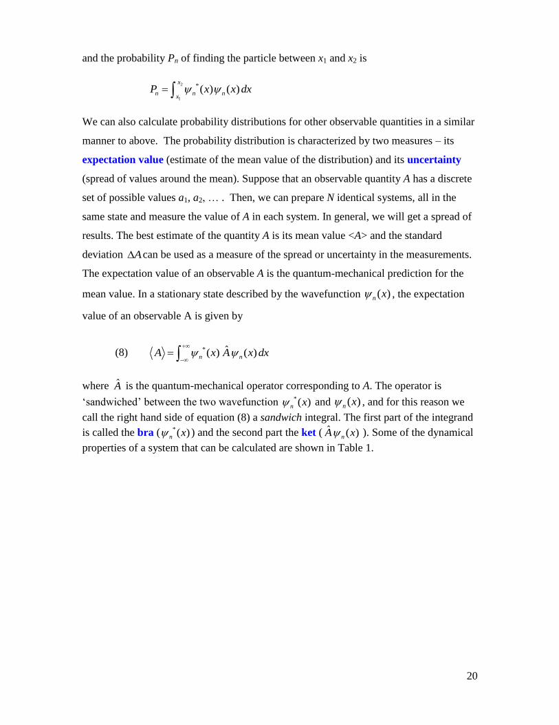
The expectation value of an observable A is the quantum-mechanical prediction for the
mean value. In a stationary state described by the wavefunction ( )n x , the expectation
value of an observable A is given by
(8) * ˆ( ) ( )n nA x A x dx
where A is the quantum-mechanical operator corresponding to A. The operator is
‘sandwiched’ between the two wavefunction *( )n x and ( )n x , and for this reason we
call the right hand side of equation (8) a sandwich integral. The first part of the integrand
is called the bra ( *( )n x ) and the second part the ket ( ˆ ( )nA x ). Some of the dynamical
properties of a system that can be calculated are shown in Table 1.
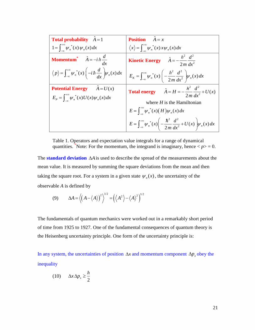
21
Total probability ˆ 1A
*1 ( ) ( )n nx x dx
Position A x
*( ) ( )n nx x x x dx
Momentum* ˆ d
A idx
*( ) ( )n n
dp x i x dx
dx
Kinetic Energy 2 2
2ˆ
2
dA
m dx
2 2*
2( ) ( )
2K n n
dE x x dx
m dx
Potential Energy ˆ ( )A U x
*( ) ( ) ( )P n nE x U x x dx
Total energy 2 2
2ˆ ( )
2
dA H U x
m dx
where H is the Hamiltonian
*
2 2*
2
( ) ( )
( ) ( ) ( )2
n n
n n
E x H x dx
dE x U x x dx
m dx
Table 1. Operators and expectation value integrals for a range of dynamical
quantities. *Note: For the momentum, the integrand is imaginary, hence < p> = 0.
The standard deviation A is used to describe the spread of the measurements about the
mean value. It is measured by summing the square deviations from the mean and then
taking the square root. For a system in a given state ( )n x , the uncertainty of the
observable A is defined by
(9) 1/2 1/22 22A A A A A
The fundamentals of quantum mechanics were worked out in a remarkably short period
of time from 1925 to 1927. One of the fundamental consequences of quantum theory is
the Heisenberg uncertainty principle. One form of the uncertainty principle is:
In any system, the uncertainties of position x and momentum component xp obey the
inequality
(10) 2
xx p
22
Hence, it is impossible to find a state in which a particle has both definite values for
position and momentum. The classical picture of a particle following a well-defined
trajectory is no longer valid. A system described by a wavefunction implies a spread of
position and momentum values and that a narrow spread in one of these quantities is
offset by a wide spread in the other. The uncertainty principle is sometimes interpreted in
terms of the disturbance produced by a measurement, but, this is not correct. The
uncertainty principle tells us about the indeterminacy that is inherent in a given state
before the measurement is made.
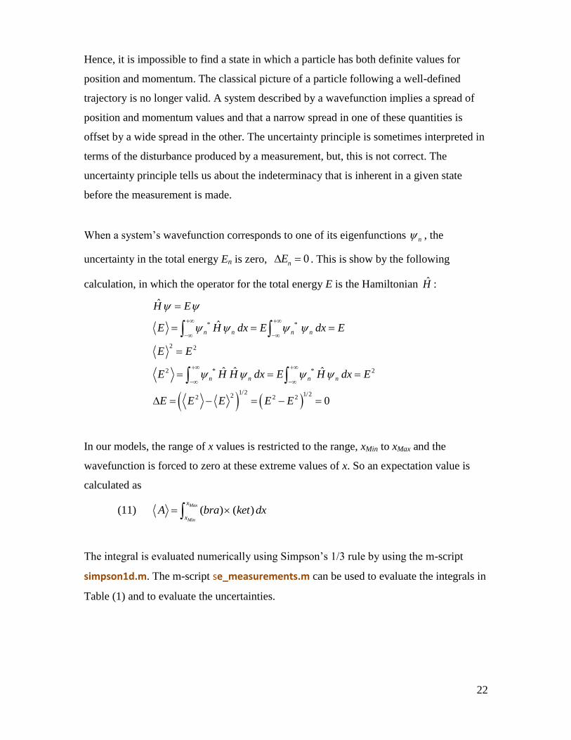
When a system’s wavefunction corresponds to one of its eigenfunctions n , the
uncertainty in the total energy En is zero, 0nE . This is show by the following
calculation, in which the operator for the total energy E is the Hamiltonian H :
* *
2 2
2 * * 2
1/2 1/222 2 2
ˆ
ˆ
ˆ ˆ ˆ
0
n n n n
n n n n
H E
E H dx E dx E
E E
E H H dx E H dx E
E E E E E
In our models, the range of x values is restricted to the range, xMin to xMax and the
wavefunction is forced to zero at these extreme values of x. So an expectation value is
calculated as
(11) ( ) ( )Max
Min
x
xA bra ket dx
The integral is evaluated numerically using Simpson’s 1/3 rule by using the m-script
simpson1d.m. The m-script se_measurements.m can be used to evaluate the integrals in
Table (1) and to evaluate the uncertainties.
23
Sample codes from the m-script se_measurements.m to evaluate the expectation value
for total energy and the uncertainty in position are:
% total energy – need to convert units in calculations
psi1 = gradient(Psi,x); ket = - (hbar^2/(2*me*e))*gradient(psi1,x)(Lse^2*Ese) + (U.*Psi')'; braket = bra .* ket; Eavg = simpson1d(braket,xMin,xMax);
% position x & uncertainty in position ket = x .* Psi;
braket = bra .* ket; xavg = simpson1d(braket,xMin,xMax);
ket = (x.^2) .* Psi; braket = bra .* ket; x2avg = simpson1d(braket,xMin,xMax);
deltax = sqrt(x2avg - xavg^2) * Lse; % length units nm to m
The m-script se_measurements.m outputs numerical values of the integrals to the
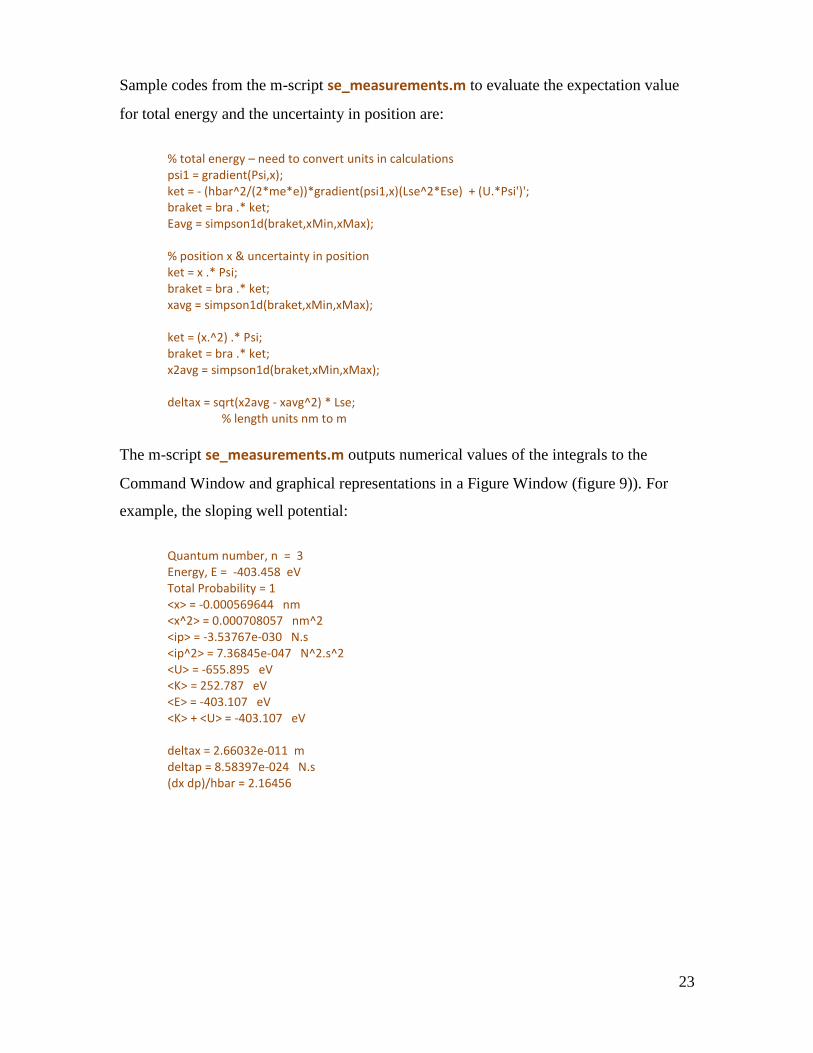
Command Window and graphical representations in a Figure Window (figure 9)). For
example, the sloping well potential:
Quantum number, n = 3 Energy, E = -403.458 eV Total Probability = 1 <x> = -0.000569644 nm <x^2> = 0.000708057 nm^2 <ip> = -3.53767e-030 N.s <ip^2> = 7.36845e-047 N^2.s^2 <U> = -655.895 eV <K> = 252.787 eV <E> = -403.107 eV <K> + <U> = -403.107 eV deltax = 2.66032e-011 m deltap = 8.58397e-024 N.s (dx dp)/hbar = 2.16456
24
From the above result, we can conclude the following:
1 E = < E > ignoring the slight difference in numerical values due to numerical
inaccuracies in our modeling.
2 < E > = < K > + < U >
3 The average position of the electron is slightly to the left of the origin.
4 The uncertainty principle is satisfied 2.2 0.5x p
.
5 The expectation for momentum is complicated by the factor i and so we have to
calculate < i p > which is then a real quantity and from the results above, we can
conclude that <i p> = 0. No measurable physical quantity can be imaginary, hence
the integral must be zero.
It is remarkable that a bound particle has definite set of discrete values for its total energy
and this follows simply and directly from applying boundary conditions to a
wavefunction that satisfies the Schrodinger Equation. At first, it seems surprising that the
total energy has a set of unique values ( 0E ) but the momentum does not, since the
uncertainty principle must be satisfied. But a classical vibrating string in a normal mode
has a unique frequency of vibration while not possessing a unique wavelength as the
transverse standing wave is sinusoidal along the string but is zero at and outside the fixed
end points. However, the shape of the string inside and outside the fixed ends can be
thought of a superposition of waves of different wavelengths with amplitudes and phases
chosen so that the disturbance cancels everywhere except in the region between the end
points. Therefore, the wavefunction can be thought of a superposition of different
wavelengths and through the de Broglie relationship /p h ,the confined particle has a
range of momentum.
25
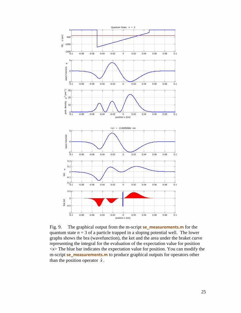
Fig. 9. The graphical output from the m-script se_measurements.m for the
quantum state n = 3 of a particle trapped in a sloping potential well. The lower
graphs shows the bra (wavefunction), the ket and the area under the braket curve
representing the integral for the evaluation of the expectation value for position
<x> The blue bar indicates the expectation value for position. You can modify the
m-script se_measurements.m to produce graphical outputs for operators other
than the position operator x .
-0.1 -0.08 -0.06 -0.04 -0.02 0 0.02 0.04 0.06 0.08 0.1-1500
-1000
-500
0
PE
,
U (
eV
)
Quantum State, n = 3
-0.1 -0.08 -0.06 -0.04 -0.02 0 0.02 0.04 0.06 0.08 0.1-5
0
5
wave f
unction,
-0.1 -0.08 -0.06 -0.04 -0.02 0 0.02 0.04 0.06 0.08 0.10
10
20
30
position x (nm)
pro
b.
density,
2 (
nm
-1)
-0.1 -0.08 -0.06 -0.04 -0.02 0 0.02 0.04 0.06 0.08 0.1-5
0
5
wave f
unction
<x> = -0.00056964 nm
-0.1 -0.08 -0.06 -0.04 -0.02 0 0.02 0.04 0.06 0.08 0.1-0.2
-0.1
0
0.1
0.2
ket,
-0.1 -0.08 -0.06 -0.04 -0.02 0 0.02 0.04 0.06 0.08 0.1-1
-0.5
0
0.5
bra
ket
position x (nm)
26
ACCUARY OF THE NUMERICAL MODELLING
Numerical results may not always be accurate. Where possible you need to check that the
results are OK. Firstly, you should always vary the number of points used in the
modeling. In solving the Schrodinger Equation by the Matrix Method, the variable num
which is set in the m-script se_wells.m determines the size of the vectors and arrays.
Generally, if this number is too low the results are not accurate. You should start with a
small number for num and increase it until there is a convergence in the results. If num is
too large, then the execution time in running the m-scripts could be excessive and/or too
much memory is used. Secondly, if possible you should compare the predictions of a
numerical method with the known results predicted by analytical methods. The energy
eigenvalues for an infinite square well can be easily found analytically, so we can
compare those results with our numerical model.
Consider a system with an electron of mass me confined to a one dimensional region of
length L. The potential well called an infinite square well has infinitely high walls which
trap the particle, but the force on the electron is zero between the walls. The potential
energy function and boundary conditions on the wavefunctions are
( ) 0 / 2 / 2
( ) / 2 and / 2
( / 2) 0 ( / 2) 0
U x L x L
U x x L x L
L L
The classical predictions for such a system, is that the total energy of the trapped particle
can have any positive value and since the potential energy inside the well is zero, the
kinetic energy of the particle equals the total energy. The particle can have zero total
energy (zero kinetic energy) and if its kinetic energy is greater than zero the particle will
bounce back and forth between the impenetrable walls with constant speed. Increasing
the energy simply increases the speed but no matter how great the speed, the particle
can’t be outside the walls, the region outside the walls is said to be classically forbidden.
27
The predictions of quantum mechanics are very different. In solving of the Schrodinger
Equation it is found that the shape of the wavefunction inside the walls is sinusoidal and
the wavefunction must be zero at the walls since the potential energy is infinite at each
wall. Therefore, the only acceptable physical solutions are those wavefunctions where
integer multiple of half-wavelengths of a sine curve fit into the distance L between the
walls:
2
1,2,3,2
LL n n
n
The total energy E is related to the momentum p and the momentum related to a
wavelength (de Broglie relationship) hence, we can determine an expression for the
total energy as a function of n (principle quantum number) and the length L
22
2
L h pp E
n m
(12) 2
2
21,2,3,
8n
hE n n
m L
This is a momentous result and very different from the predictions of classical physical.
The principle quantum number n is restricted to integer values, therefore, the bound
particle has only a discrete set of values for its total energy and these are the only possible
values for the total energy of the system. The lowest value is n = 1, and the lowest
allowed energy is 2 2
1 / 8 0E h m L . No particle in an infinite square well can have an
energy lower than this, there is no state of zero total energy. This energy is called the
ground state energy. If L then the spacing between energy 0E which implies
that the particle is behaving more like a free classical particle which can have any
positive energy.
28
We can compare the predictions from the analytical model and the Matrix Method for an
electron confined to an infinite square well potential of width 0.1 nm. To use the Matrix
Method, modify m-script se_wells.m to produce an infinite square well potential then run
it:
Infinite square well parameters set in se_wells.m
num = 801
Option 1 (case 1) square well
xMin = -0.05
xMax = +0.05
U1 = 0
Then run the m-scipt se_solve.m. The screen output states that no eigenvalues are found.
This is because the code is expecting negative values for the total energy. However, we
can extract the required values for the total energy manually using the command
e_values(mm,mm) in the Command Window. Do this and record the first 10 eigenvalues
for mm = 1, 2, … , 10. These values are stored in the m-script se_infwells.m. Run the m-
script se_infWells.m. Note, when this file is run, all variables are cleared from the
workspace. The file se_infWells.m calculates the first 10 energy levels using equation
(12), outputs the results to the Command Window and plots the numerical and analytical
values in a Figure Window (figure 10):
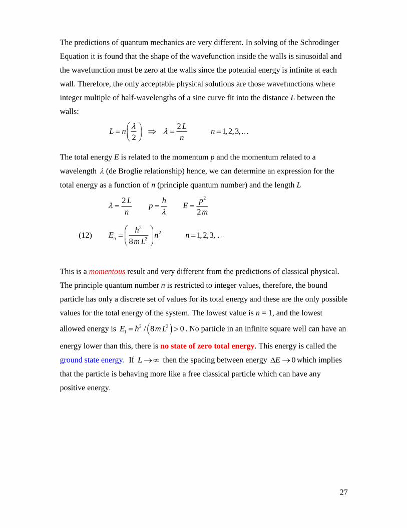
n E (eV) Emm (eV) 1 37.74 37.69 2 150.95 150.74 3 339.64 339.17 4 603.80 602.97 5 943.44 942.13 6 1358.56 1356.60 7 1849.15 1846.50 8 2415.21 2411.70 9 3056.76 3052.30 10 3773.77 3768.10
29
Fig. 10. The energy eigenvalues for an infinite square well of width 0.10
nm calculated from equation (12) and the Matrix Method using the m-
scripts se_wells.m and se_solve.m. [se_infWell.m]
The discrepancy between the two sets of results is better than 0.2%. Therefore, we can
have some confidence in the results from the Matrix Method for other potential well
functions.
The wavefunctions for the infinite square well can be plotted after running se_solve.m by
typing the following commands in the Command Window, for example, to display the
eigenvector for the state n = 8
plot(e_funct(:,8),'lineWidth',3) axis off
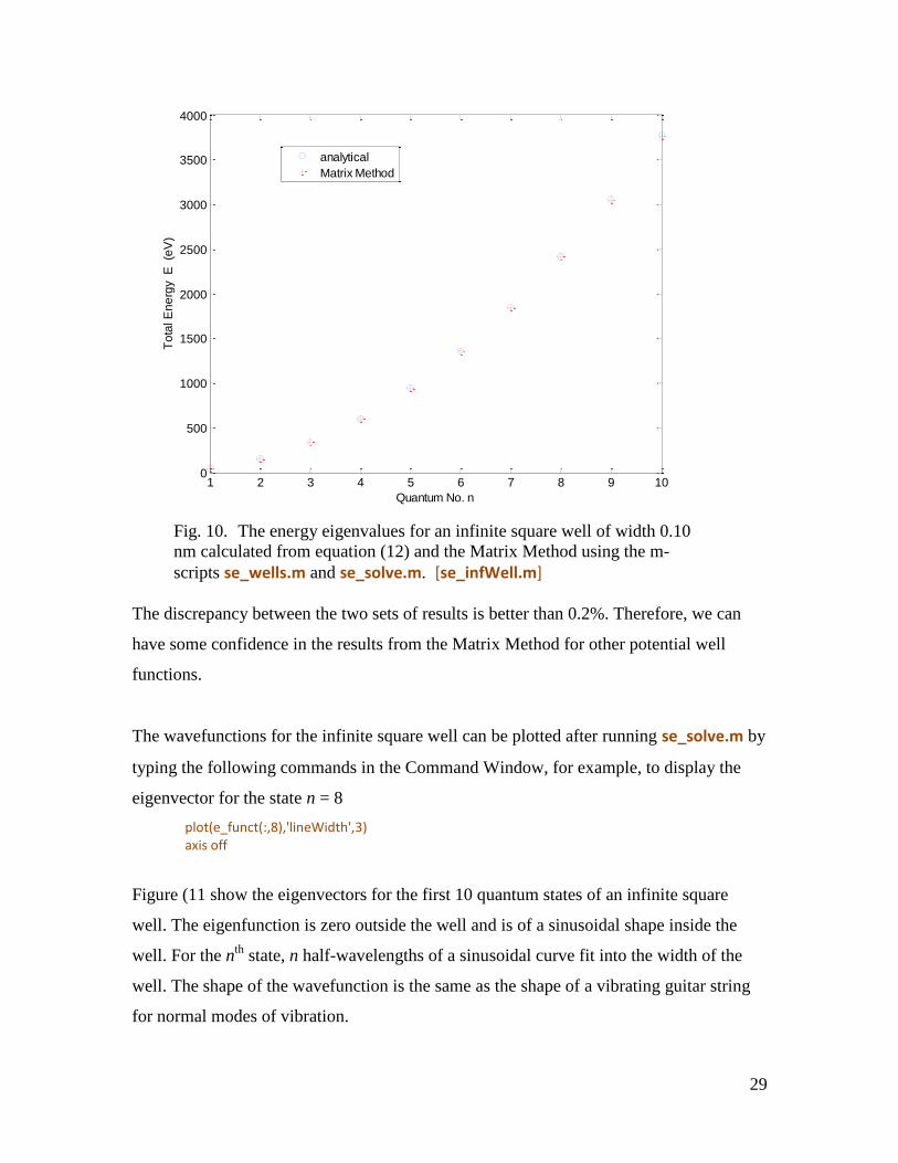
Figure (11 show the eigenvectors for the first 10 quantum states of an infinite square
well. The eigenfunction is zero outside the well and is of a sinusoidal shape inside the
well. For the nth
state, n half-wavelengths of a sinusoidal curve fit into the width of the
well. The shape of the wavefunction is the same as the shape of a vibrating guitar string
for normal modes of vibration.
1 2 3 4 5 6 7 8 9 100
500
1000
1500
2000
2500
3000
3500
4000
Quantum No. n
To
tal E
ne
rgy E
(e
V)
analytical
Matrix Method
30
Fig. 11. The energy eigenvectors for an infinite square well for the first 10
quantum states. [se_wells.m se_solve.m]
When a potential well is of finite depth, the wavefunction extends into the classically
forbidden region and so there is some probability of finding the particle outside the well
which in classical terms in impossible. For a particular state of an infinite square well, the
wavelength is constant (independent of x). This is not the case when the potential inside
the well changes with x, for example, the wavelength increases with decreasing potential
in the sloping well (figures 8 & 9) and so the shape of the wavefunction is not simply
sinusoidal.
1 2
4 5 6
7 8 9 10
3
31
INVESTIGATIONS (Matrix Method)
There are many aspects of quantum behavior for bound states you can investigate by
studying various potential wells with different parameters. A proven learning strategy
that you can apply to gain a deeper understanding of quantum physics is called POE
Predict Observe Explain
For a given potential well, some of the predictions you could make are: number of bound
states, approximate values of energy eigenvalues, spacing of energy levels, shape of
wavefunction, number of half-wavelengths inside well, changes in half-wavelengths and
size of exponential tails, the number of zero crossings of the wavefunction, and height of
peaks in wavefunction. For example, in a square well the energy levels are more crowded
towards the bottom of the well, in a parabolic well (shape bends away from x-axis) the
energy levels are equally spaced and in the Morse potential well or a Coulomb shaped
well (shape bends towards the x-axis) the energy levels are more crowed toward the top
of the potential well.
After you have made your predictions, run the m-scripts and observe the results and
compare them with your predictions.
Then, you explain the results you observed and rectify any discrepancies in the results
and your predictions.
32
1 Infinite Square Well and Finite Square Well
1.1 Find the energy eigenvalues for various widths of an infinite square well and
compare your results with theoretical values predicted by equation (12). For each
state (n = 1, 2, …. ) measure the wavelength , then using the de Broglie
relationship ( /p h ), calculate the momentum of the electron and its kinetic
energy ( 2 / 2KE p m ). Compare the energy eigenvalues with the kinetic energy
values. Repeat the calculations for different values of num (size of vectors and
arrays). Can use the m-script se_infwell.m.
1.2 Find the energy eigenvalues for various square wells of different depths and
widths. Observe the wavefunction and expectation values for different states.
Check the orthonormal character of the wavefunctions [se_othonormal]. Why
does the wavelength of the eigenfunctions decrease as the quantum number n
increases? Why is the kinetic energy of the electron in each eigenstate of a finite
square well less than the value of its kinetic energy in an infinite square well of
the same width? How does the number of zero crossing of the wavefunction vary
with the quantum number n? Comment on the curvature of the wavefunction
inside and outside of the potential well and explain. Comment on the expectation
values and is the Heisenberg Uncertainty Principle satisfied?
1.3 The simplest nuclear system is a deuteron - a single proton bound together with a
single neutron by the attractive strong nuclear force. This system has only one
bound state with a binding energy of 2.22 MeV near the top of the well. This is
the ground state, there are no excited states. This is a three dimensional system,
but we can model the strong nuclear force as a one-dimensional finite square well
potential where the solution of the Schrodinger Equation gives the radial
component of the wavefunction. Experiments on the scattering of high energy
electrons from deuterons provides evidence of the existence of a strong repulsive
core in the nuclear potential, this means that the particles avoid the centre of the
deuteron, the proton and neutron can’t get too close to each other, hence, the
radial wavefunction must approach zero towards the centre. The mass of the
bound particle is equal to the reduced mass of the system, hence
33
p n
p n
m mm
m m
m = (mp + mn ) / 2
We can alter the code for the square well potential (case 1) to model the potential
for the deuteron. The modifications are:
m = mp*mn/(mp+mn); reduced mass - deuteron xMin = 0 forces the wavefunction at the centre of the deuteron to be zero
x1 = 1.5e-6 width of square well in nm xMax = 20*x1 U1 = -100e6 starting depth of square well in eV
Find the binding energy using se_solve.m. Then, adjust the value of U1 until the
binding energy is about 2.2 MeV to find an estimate of the well depth. View the
characteristics of the wavefunction using se_psi.m. In the ground state, the
eigenfunction describing the separation of the proton and neutron extends far
beyond the confines of the well. From the Command Window determine the
probability that the separation distance between the proton and neutron is greater
than the width of the well using the function simpson1d.m:
Check that the function is normalized, use
simpson1d(prob(:,1)',xMin,xMax) result should be 1.
The probability that the electron is found within the well, use
simpson1d(prob(1:min(find(x>=x1)),1)',0,x1)
to evaluate the integral 1 1
0 0( ) ( ) ( )
x x
x x dx prob x dx . The statement
min(find(x>=x1)) finds the index of x for the edge of the well at x1.
The probability density 2( )x specifies the probability of finding the two
nucleons in the deuteron with a separation in the vicinity of x.
Use se_measurements.m to find the average separation distance.

34
One book quoted that the mean separation of the proton and neutron as
4×10-15
m (much larger than the width of the well) and that there was a 50%
chance of finding the particles in the classical forbidden region. How do your
results compare? Your results about probability imply that the attractive region for
the only bound state is just barely strong enough to overcome the effect of the
repulsive core and lead to binding. As a consequence, there is a high probability
that the two nucleons in the deuteron have a separation larger than the range of
nucleon forces. The values for xMax, x1 and U1 are not unique in giving the correct
value for the binding energy. If you check different references, you will get
different numbers quoted in each reference. Remember, that our model is a crude
one, and the numbers are not necessary accurate but the model does give an
insight to the deuteron nucleus.
2 Stepped Well (Asymmetrical Well)
2.1 Investigate the solutions of the Stepped Well for various widths and depths of the
left and right sides of the well by modifying the code in se_wells.m
case 2 xMin = -0.15; % default = -0.15 nm xMax = +0.15; % default = +0.15 nm x1 = 0.1; % Total width of well: default = 0.1 nm x2 = 0.06; % Width of LHS well: default = 0.06 nm; U1 = -400; % Depth of LHS well; default = -400 eV; U2 = -200; % Depth of RHS well (eV); default = -250 eV;
Set U1 = -400, U2 = -200, x1 = 0.10 and x2 = 0, 0.25x1, 0.50x1, 0.75x1, 1.00x1
Set x1 = -0.10, x2 = -0.05, U1 = -400 and U2 = 0, 0.25U1, 0.50U1, 0.75U1, 1.00U1
2.2 Investigate an asymmetrical well by commenting the line as shown below in the
m-script for se_wells.m (case 2).
for cn = 1 : num if x(cn) >= -x1/2, U(cn) = U1; end; %if if x(cn) >= -x1/2 + x2, U(cn) = U2; end; %if %if x(cn) > x1/2, U(cn) = 0; end; %if % comment above line to give an asymmetrical well end %for
35
Fig. 12. The energy spectrum for a stepped well.
[se_wells.m se_solve.m]
Fig. 13. The quantum state n = 3 for a stepped well.
[se_wells.m se_solve.m se_psi.m]
-0.15 -0.1 -0.05 0 0.05 0.1 0.15-450
-400
-350
-300
-250
-200
-150
-100
-50
0
50
position x (nm)
en
erg
y U
, E
n (
eV
)
Potential Well: STEPPED
-0.15 -0.1 -0.05 0 0.05 0.1 0.15-10
0
10
Potential Well: STEPPED n = 3 En = -115.2244
position x (nm)
wave f
unction
psi
-0.15 -0.1 -0.05 0 0.05 0.1 0.15
-400
-200
0
U
(eV
)
-0.15 -0.1 -0.05 0 0.05 0.1 0.150
20
40
position x (nm)
pro
b d
ensity
psi?
-0.15 -0.1 -0.05 0 0.05 0.1 0.15
-400
-200
0
U
(eV
)-0.1 -0.05 0 0.05 0.1 0.15
-400
-200
0
200
En(black) U(red) K(green)
position x (nm)
energ
ies
(eV
)
36
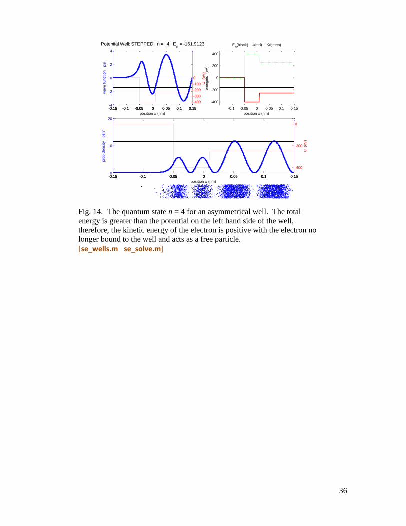
Fig. 14. The quantum state n = 4 for an asymmetrical well. The total
energy is greater than the potential on the left hand side of the well,
therefore, the kinetic energy of the electron is positive with the electron no
longer bound to the well and acts as a free particle.
[se_wells.m se_solve.m]
-0.15 -0.1 -0.05 0 0.05 0.1 0.15-4
-2
0
2
4
Potential Well: STEPPED n = 4 En = -161.9123
position x (nm)
wave f
unction
psi
-0.15 -0.1 -0.05 0 0.05 0.1 0.15
-400
-300
-200
-100
0
U
(eV
)
-0.15 -0.1 -0.05 0 0.05 0.1 0.150
10
20
position x (nm)
pro
b d
ensity
psi?
-0.15 -0.1 -0.05 0 0.05 0.1 0.15
-400
-200
0
U
(eV
)
-0.1 -0.05 0 0.05 0.1 0.15
-400
-200
0
200
400
En(black) U(red) K(green)
position x (nm)
energ
ies
(eV
)
37
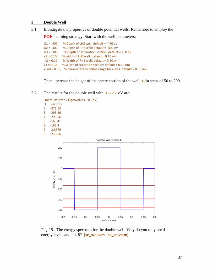
3 Double Well
3.1 Investigate the properties of double potential wells. Remember to employ the
POE learning strategy. Start with the well parameters:
U1 = -400; % Depth of LHS well: default = -440 eV U2 = -400; % Depth of RHS well: default = -400 eV U3 = -300; % Depth of separation section: default = 100 eV x1 = 0.10; % width of LHS well: default = 0.10 nm x2 = 0.10; % Width of RHS well: default = 0.10 nm x3 = 0.10; % Width of separtion section: default = 0.10 nm xEnd = 0.05; % parameters to define range for x-axis: default = 0.05 nm
Then, increase the height of the centre section of the well U3 in steps of 50 to 200.
3.2 The results for the double well with U3 = 200 eV are:
Quantum State / Eigenvalues En (eV) 1 -373.13 2 -373.13 3 -293.56 4 -293.56 5 -165.41 6 -165.4 7 -2.8576 8 -2.7866
Fig. 15. The energy spectrum for the double well. Why do you only see 4
energy levels and not 8? [se_wells.m se_solve.m]
-0.2 -0.15 -0.1 -0.05 0 0.05 0.1 0.15 0.2
-400
-300
-200
-100
0
100
200
position x (nm)
en
erg
y U
, E
n (
eV
)
Potential Well: DOUBLE
38
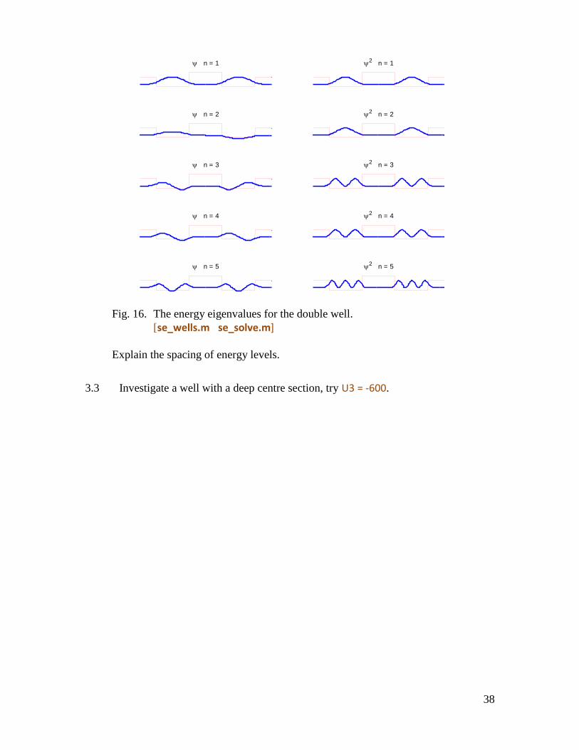
Fig. 16. The energy eigenvalues for the double well.
[se_wells.m se_solve.m] Explain the spacing of energy levels.
3.3 Investigate a well with a deep centre section, try U3 = -600.
n = 1 2 n = 1
n = 2 2 n = 2
n = 3 2 n = 3
n = 4 2 n = 4
n = 5 2 n = 5
39
4 Sloping Well
4.1 Investigate the properties of sloping potential wells. Remember to employ the
POE learning strategy.
5 Truncated Parabolic Well
5.1 Investigate the properties of truncated parabolic potential wells. Remember to
employ the POE learning strategy. What can you say about the spacing between
energy levels?
5.2 The potential energy for a classical particle oscillating in a parabolic well (e.g.
particle vibrating at the end of a spring executing simple harmonic motion) is
212
( ) sU x k x where ks is the spring constant.
The eigenstates for this system are the solutions of the Schrodinger Equation:
2 2
2122
( ) ( )2
s n sn n
dk x x E x
m dx
The energy eigenvalues for this system known as the quantum harmonic
oscillator are given by
12snE n
where n = 1, 2, 3, … (N.B. most books have n = 0, 1, 2, 3, … )
The classical frequency of oscillation for a particle of mass m is
2s sk kf
m m
The Schrodinger Equation for our truncated parabolic well is
22 2
112 2
1
1 4 ( ) ( )2
n sn n
UdU x E x
m dx x
where U1 is the depth of the well and x1 is the full width of the well when U = 0.
Show that the spring constant ks is related to the well parameters U1 and x1 by the
relationship
1
2
1
8s
Uk
x
40
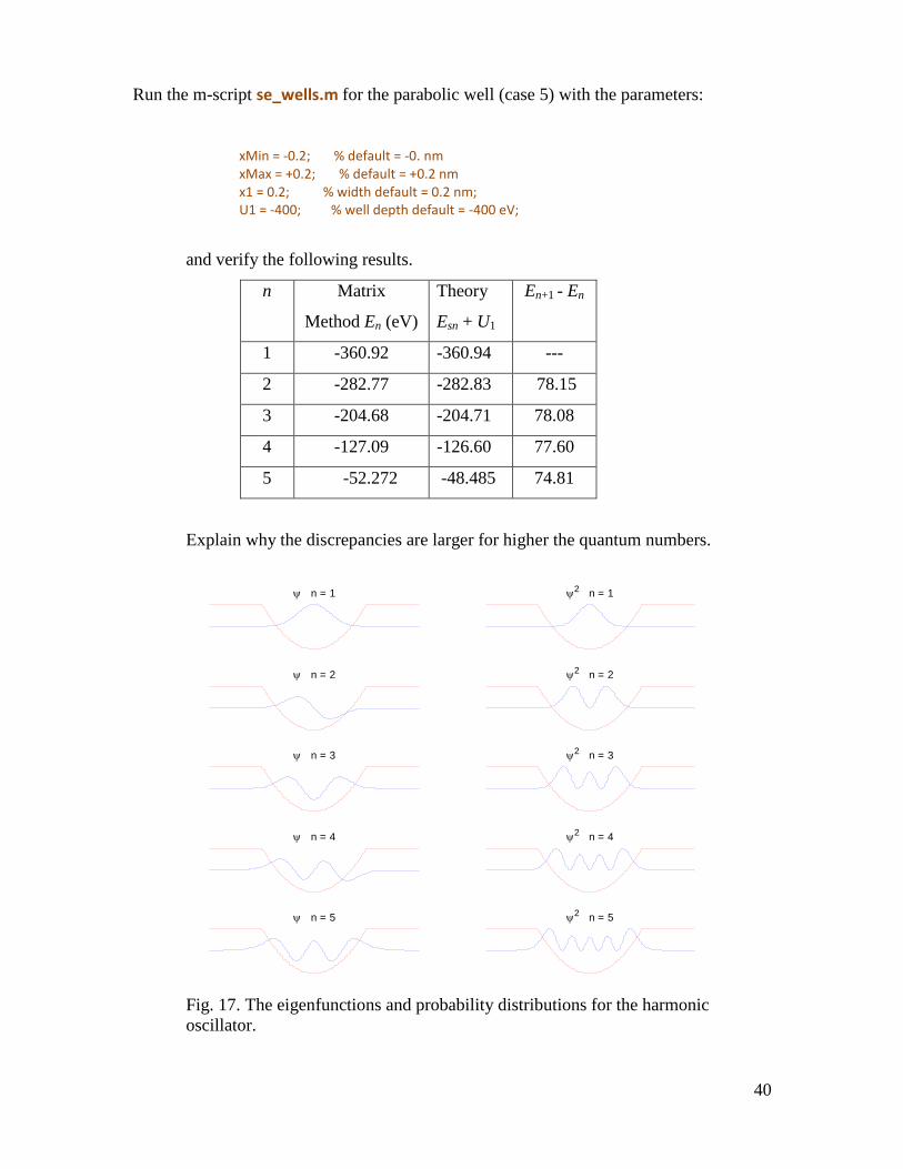
Run the m-script se_wells.m for the parabolic well (case 5) with the parameters:
xMin = -0.2; % default = -0. nm xMax = +0.2; % default = +0.2 nm x1 = 0.2; % width default = 0.2 nm; U1 = -400; % well depth default = -400 eV;
and verify the following results.
n Matrix
Method En (eV)
Theory
Esn + U1
En+1 - En
1 -360.92 -360.94 ---
2 -282.77 -282.83 78.15
3 -204.68 -204.71 78.08
4 -127.09 -126.60 77.60
5 -52.272 -48.485 74.81
Explain why the discrepancies are larger for higher the quantum numbers.
Fig. 17. The eigenfunctions and probability distributions for the harmonic
oscillator.
n = 1 2 n = 1
n = 2 2 n = 2
n = 3 2 n = 3
n = 4 2 n = 4
n = 5 2 n = 5
41
Explain why the state n = 5 in figure (17) is more like the classical prediction for
the probability of locating the particle.
5.2 Repeat the above, for different well parameters. Run se_measurements.m and
find the expectation values for a number of states. What is the significance for the
state n =1 by considering the value for x p ?
42
6 Morse Potential Well
6.1 Investigate the properties of Morse parabolic potential wells. Remember to
employ the POE learning strategy. What can you say about the spacing between
energy levels?
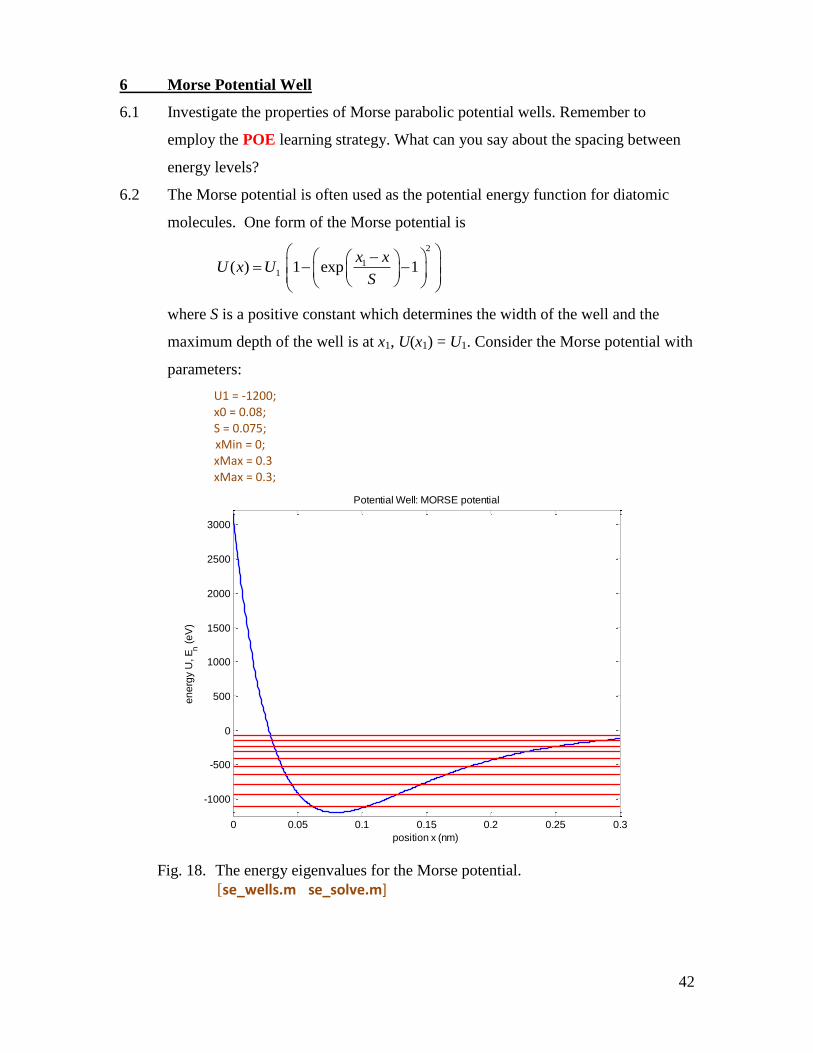
6.2 The Morse potential is often used as the potential energy function for diatomic
molecules. One form of the Morse potential is
2
11( ) 1 exp 1
x xU x U
S
where S is a positive constant which determines the width of the well and the
maximum depth of the well is at x1, U(x1) = U1. Consider the Morse potential with
parameters:
U1 = -1200; x0 = 0.08; S = 0.075; xMin = 0; xMax = 0.3 xMax = 0.3;
Fig. 18. The energy eigenvalues for the Morse potential.
[se_wells.m se_solve.m]
0 0.05 0.1 0.15 0.2 0.25 0.3
-1000
-500
0
500
1000
1500
2000
2500
3000
position x (nm)
en
erg
y U
, E
n (
eV
)
Potential Well: MORSE potential

43
Run the m-script se_measurements.m and record the expectation value
for position. Comment on the spacing of the energy levels and explain why
most materials expand upon heating.