doing physics with matlab resonance circuits rlc … · 1 doing physics with matlab resonance...

1

DOING PHYSICS WITH MATLAB

RESONANCE CIRCUITS

RLC PARALLEL VOLTAGE DIVIDER

Matlab download directory

Matlab scripts

CRLCp1.m CRLCp2.m

When you change channels on your television set, an RLC circuit is used to

select the required frequency. To watch only one channel, the circuit must

respond only to a narrow frequency range (or frequency band) centred

around the desired one. Many combinations of resistors, capacitors and

inductors can achieve this. We will consider a RLC voltage divider circuit

shown in figure 1. The circuit shown in figure 1 can also be used as a

narrow band pass filter or an oscillator circuit.

http://www.physics.usyd.edu.au/teach_res/mp/mphome.htm

http://www.physics.usyd.edu.au/teach_res/mp/mscripts/

2

Fig. 1. RLC resonance circuit: a parallel combination of an

inductor L and a capacitor C used in voltage divider circuit.

The sinusoidal input voltage is

ej t

INV

The impedances of the circuits components are

1 1

Z R series resistance

2 OUT

Z R output or load resistance

3

jZ

C

capacitor

4 L

Z R j L inductor

3

We simplify the circuit by combining circuit elements that are in series and

parallel.

5

2 3 4

1

1 1 1Z

Z Z Z

parallel combination

6 1 5

Z Z Z series combination: total impedance

The current through each component and the potential difference across

each component is computed from

V

I V I ZZ

in the following sequence of calculations

1

6

1 1 1

1

2 3 4

2 3 4

IN

OUT IN

OUT OUT OUT

VI

Z

V I Z

V V V

V V VI I I

Z Z Z

Computing all the numerical values is easy using the complex number

commands in Matlab. Complex circuits can be analysed and in more in-

depth graphically than the traditional algebraic approach.

The code below shows the main calculations that needed for the

simulations.

4

f = linspace(fMin,fMax, N);

w = (2*pi).*f;

% impedances

Z1 = RS; % series resistance

Z2 = ROUT; % output or load resistance

Z3 = -1i ./ (w .*C); % capacitive impedance

Z4 = RL + 1i .* w .* L; % inductive impedance

(resistance + reactance)

Z5 = 1./ (1./Z2 + 1./Z3 + 1./Z4); % parallel combination

Z6 = Z1 + Z5; % total circuit

impedance

% currents [A] and voltages [V]

I1 = V_IN ./ Z6;

V1 = I1 .* Z1;

V_OUT = V_IN - V1;

I2 = V_OUT ./ Z2;

I3 = V_OUT ./ Z3;

I4 = V_OUT ./ Z4; I_sum = abs(I1 - I2 - I3 - I4);

% phases

phi_OUT = angle(V_OUT);

phi_1 = angle(V1);

theta_1 = angle(I1);




% Resonance frequencies and Bandwidth calculations

f0 = 1/(2*pi*sqrt(L*C));

G_V = abs(V_OUT ./ V_IN); % voltage gain

Vpeak = max(G_V); % max voltage gain

VG3dB = Vpeak/sqrt(2); % 3 dB points

k = find(G_V == Vpeak); % index for peak voltage gain

f_peak = f(k); % frequency at peak

kB = find(G_V > VG3dB); % indices for 3dB peak

k1 = min(kB); f1 = f(k1);

k2 = max(kB); f2 = f(k2);

df = f2-f1; % bandwidth

Q = f0 / df; % quality factor

P_OUT = V_OUT .* I2; % power delivered to load

5

We will consider the following example that was done as an experiment

and as a computer simulation.

Values for circuit parameters:

amplitude of input emf 10.0Vin

V

series resistance 41.00 10

SR

capacitance 910.4 10 F (10 nF)C

inductance 310.3 10 H (10 mH)L

inductance resistance estimated from simulation

output (load) resistance 61.00 10

OUTR (output to CRO)

Simulation 0L

R script CRLCp1.m

% ==============================================================

% INPUTS default values [ ]

% ==============================================================

% series resistance Z1 [1e4 ohms]

RS = 1e4;

% OUTPUT (LOAD) resistance Z2 [1e6 ohms]

ROUT = 1e6;

% inductance and inductor resistance Z4 [10.3e-3 H 0 ohms]

L = 10.3e-3;

RL = 0;

% capacitance Z2 [10.4e-9 F]

C = 10.4e-9;

% input voltage emf [10 V]

V_IN = 10;

% frequency range [1000 to 30e3 Hz 5000]

fMin = 1000; fMax = 30e3;

N = 5000;

6

Figure 2 shows the plots of the absolute values for the impedance of the

capacitor 3Z , inductor 4

Z and output impedance for the parallel

combination 5Z .

At low frequencies, the inductor acts like a “short circuit”

4

40 0 0

L

out

Z Z j L

f Z Z

At high frequencies, the capacitor acts like a “short circuit”

3

30 0 0

C

out

jZ Z

C

f Z Z

At resonance L CZ Z

1

LC

resonance frequency 0 0

1 1

2f

LC LC

The output impedance 5out

Z Z has a sharp peak at the resonance

frequency 0

f .

7

Fig. 2. The magnitude of the impedances for the capacitor,

inductor and parallel combination as functions of frequency of

the source. A sharp peak occurs at the resonance frequency for

the impedance of the parallel combination.

8

Since the total circuit impedance has a maximum value at the resonance,

the current from the source must be a minimum at the resonance

frequency (figure 3). At resonance, the source voltage and the source

current are in-phase with each other and the current through the series

resistance is the same as the current through the output resistance.

Fig. 3. The source current has a minimum at the resonance

frequency. At resonance, the source voltage and source current

are in-phase with each other.

9

The output voltage from the parallel combination is

OUTj t

OUT OUTv V e

We define the voltage gain V

G of the circuit as

OUTV

IN

VG

V

The V

G is a complex quantity which is specified by its magnitude and

phase. Figure 4, shows the magnitude of the voltage gain V

G and its phase

OUT . The voltage gain

VG has a peak at the resonance frequency and the

output voltage OUT

v is in phase with the source voltage since 0OUT .

Fig. 4. The voltage gain V

G of the parallel voltage divider

resonance circuit.

10

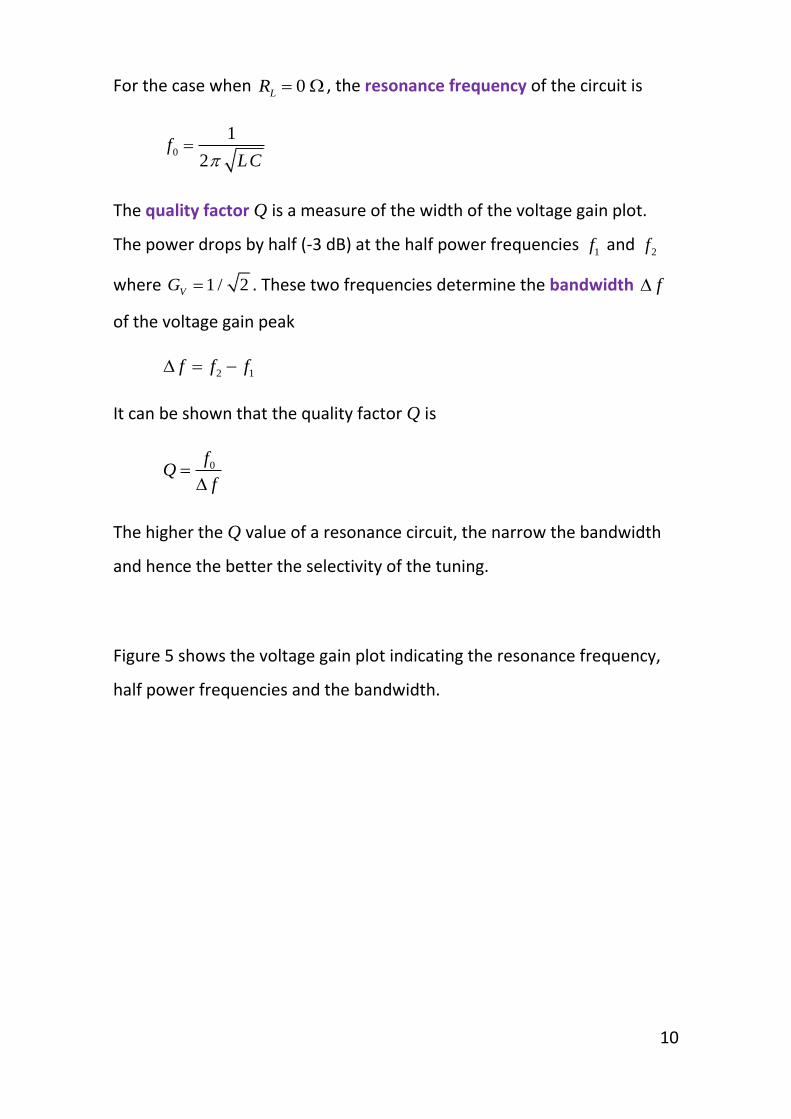
For the case when 0L

R , the resonance frequency of the circuit is

0

1

2f

LC

The quality factor Q is a measure of the width of the voltage gain plot.

The power drops by half (-3 dB) at the half power frequencies 1

f and 2

f

where 1 / 2V

G . These two frequencies determine the bandwidth f

of the voltage gain peak

2 1

f f f

It can be shown that the quality factor Q is

0f

Qf

The higher the Q value of a resonance circuit, the narrow the bandwidth

and hence the better the selectivity of the tuning.

Figure 5 shows the voltage gain plot indicating the resonance frequency,

half power frequencies and the bandwidth.

11

Fig. 5. The voltage gain plot indicating the resonance

frequency, half power frequencies and the bandwidth.

A summary of the calculations is displayed in the Command Window

Resonance frequency 0

15377 Hzf

Peak frequency 15375 Hzpeak

f

Half power frequencies 1 2

14627 Hz 16164 Hzf f

Quality factor 10Q

% =======================================================

% OUTPUTS IN COMMAND WINDOW

% =======================================================

fprintf('theoretical resonance frequency f0 = %3.0f Hz \n',f0);

fprintf('peak frequency f_peak = %3.0f Hz \n',f_peak);

fprintf('half power frequencies f1 = %3.0f Hz %3.0f Hz \n',f1,f2);

fprintf('bandwidth df = %3.0f Hz \n',df);

fprintf('quality factor Q = %3.2f \n',Q);

fprintf('current at junction I_sum = %3.2f mA \n',max(1e3*I_sum))

12

Figure 6 shows the magnitudes of the currents through the capacitor and

inductor branches of the parallel combination and the corresponding

phases.

For frequencies less than the resonance frequency, current through the

inductive branch is greater than through the capacitive branch. At

resonance, the two currents are equal. Above the resonance frequency,

there is more current in the capacitive branch than the inductive branch.

The two currents are always rad out of phase. The capacitive current

leads by / 2 rad while the inductive current lags by / 2 rad , compared

with the reference angle of the source emf.

At resonance, / 2 rad / 2 radC L and the two currents have

the same magnitudes. Therefore, the effects of the capacitance and

inductance cancel each other, resulting in a pure resistive impedance with

the source voltage and current in phase.

13

Fig. 6. Magnitudes and phases for the inductor current and inductor

current.

14

Kirchhoff’s current law states that the sum of the currents at a junction

add to zero. For ac circuits, it is not so straight forward to sum the

currents because you must account for the phases of each current. At the

junction of the series resistance and the parallel combination, the

simulation gives the result

1 2 3 4

0I I I I I need to account for phase

script: I_sum = abs(I1 - I2 - I3 - I4);

output: current at junction I_sum = 0.00 mA

Maximum power P vi is delivered from the source to the load only at

the resonance frequency as shown in figure 7.

Fig. 7. Power delivered from source to load.

15

We can also look at the behaviour of the circuit in the time domain and

gain a better understanding of how complex numbers give us information

about magnitudes and phases. The time domain equation for the currents

and voltages are

1

1

2

3

4

1 1

1 1

2 2

3 3

4 4

e

OUT

j t

IN

j t

j t

OUT OUT

j t

S

j t

OUT

j t

C

j t

L

V

v V e

v V e

i i I e

i i I e

i i I e

i i I e

Each of the above relationship are plotted at a selected frequency which is

set within the script. The graphs below are for the resonance frequency

and the half-power frequencies.

% ==============================================================

% TIME DOMAIN select source frequency

% =============================================================

fs = f_peak; kk = k;

% fs = f1; kk = k1;

% fs = f2; kk = k2;

Ns = 500;

ws = 2*pi*fs;

Ts = 1/fs;

tMin = 0;

tMax = 3*Ts;

t = linspace(tMin,tMax,Ns);

emf = real(V_IN .* exp(1j*ws*t));

v_OUT = real(abs(V_OUT(kk)) .* exp(1j*(ws*t + phi_OUT(kk))));

v1 = real(abs(V1(kk)) .* exp(1j*(ws*t + phi_1(kk))));

i1 = real(abs(I1(kk)) .* exp(1j*(ws*t + theta_1(kk))));




16

Fig. 8. The voltages at the resonance frequency. The source voltage and

output voltage are in-phase. The output voltage is almost equal in

magnitude to the source emf.

Fig. 9. The currents through the capacitor and inductor cancel at

resonance. The currents through the capacitor and the inductor are rad

out-of-phase and have equal amplitudes. The impedance of the circuit is

purely resistive at the resonance frequency. The output current varies

sinusoidally but has a very small amplitude.

17

Fig. 10. The voltages at the half-power frequency1

f . The source voltage

and output voltage are out-of-phase. At each instant 1 OUT

emf v v .

Fig. 11. The currents at the half-power frequency1

f . The currents

through the capacitor and the inductor are rad out-of-phase. The

amplitude of the inductor current is greater than the amplitude of the

capacitor current. The output current varies sinusoidally but has a very

small amplitude. At each instant S OUT C L

i i i i

18

Fig. 12. The voltages at the half-power frequency2

f . The source voltage

and output voltage are out-of-phase. At each instant 1 OUT

emf v v .

Fig. 13. The currents at the half-power frequency2

f . The currents

through the capacitor and the inductor are rad out-of-phase. The

amplitude of the inductor current is less than the amplitude of the

capacitor current. The output current varies sinusoidally but has a very

small amplitude. At each instant S OUT C L

i i i i

19

The above simulation has for a large impedance load connected to the

output of the circuit 61.00 10

OUTR . We can examine the effect when

a much smaller load resistance is connected to the circuit while keeping all

other parameters unchanged.

41.00 10

OUTR

Fig. 14. The voltage gain is much reduced and the bandwidth increased

giving a smaller quality factor Q. The larger bandwidth and smaller Q

means that the selectivity is of the resonance circuit is reduced.

Fig. 15. Left 41.00 10

OUTR Right 6

1.00 10OUT

R

20

Since the output resistance is reduced, a much greater output current

results and more power is delivered from the source to the load as shown

in figure 16. With 61.00 10

OUTR the maximum power at resonance

is 0.1 mW, whereas when 41.00 10

OUTR , the maximum power at

resonance 2.5 mW.

Fig. 16. The power delivered to the load is increased as the

output resistance is decreased.

21

Modelling Experimental Data

Data was measured for the circuit shown in figure 1. An audio oscillator

was used for the source and the output was connected to digital storage

oscilloscope (DSO). The component values used were (nominal values

shown in brackets):

series resistance 41.00 10

SR

capacitance 910.4 10 F (10 nF)C

inductance 310.3 10 H (10 mH)L

assume DSO resistance 61.00 10

OUTR (output to CRO)

The measurements are given in the script CRLCp2.m

Figure 17 shows a plot of the experimental data.

Fig. 17. Plot of the experimental measurements.

22

We can use our simulation CRLCp2.m to fit theoretical curves to the

measurements and estimate the resistance of the inductor as shown in

figures 18 and 19. The value of the inductive resistance L

R is changed to

obtain the best fit between the model and the measurements.

Fig. 18. The fit of the model to the measurements with 0L

R .

015377 Hz 15379 Hz 1539 Hz 9.99

peakf f f Q

23

Fig. 19. The fit of the model to the measurements with 20.0L

R .

015377 Hz 15389 Hz 1843 Hz 8.34

peakf f f Q

The model with 20.0L

R gives an excellent fit to the measurements.

The DC resistance measurement of the coil resistance measured with a

multimeter was 12.5 .

The resonance frequency is slightly higher than predicted from the

relationship

0

1

2f

LC

The bandwidth is increased and the Q of the resonance circuit is lower.

24

If you consider the simplicity of the code in the Matlab script to model

resonance circuits, this computational approach has many advantages

compared with the traditional algebraic approach.

DOING PHYSICS WITH MATLAB

If you have any feedback, comments, suggestions or corrections

please email:

Ian Cooper School of Physics University of Sydney

[email protected]

http://www.physics.usyd.edu.au/teach_res/mp/mphome.htm

doing physics with matlab resonance circuits rlc … · 1 doing physics with matlab resonance...

Documents