modern classical physics: optics, fluids, plasmas ... · modern classical physics: optics, fluids,...

1CHAPTER ONE

Newtonian Physics: Geometric ViewpointGeometry postulates the solution of these problems from mechanics and teaches the use of the

problems thus solved. And geometry can boast that with so few principles obtained from other fields,it can do so much.

ISAAC NEWTON, 1687

1.11.1 Introduction

1.1.11.1.1 The Geometric Viewpoint on the Laws of Physics

In this book, we adopt a different viewpoint on the laws of physics than that in manyelementary and intermediate texts. In most textbooks, physical laws are expressed interms of quantities (locations in space, momenta of particles, etc.) that are measured insome coordinate system. For example, Newtonian vectorial quantities are expressed astriplets of numbers [e.g., p= (px , py , pz)= (1, 9,−4)], representing the componentsof a particle’s momentum on the axes of a Cartesian coordinate system; and tensorsare expressed as arrays of numbers (e.g.,

I=⎡⎢⎣ Ixx Ixy Ixz

Iyx Iyy Iyz

Izx Izy Izz

⎤⎥⎦ (1.1)

for the moment of inertia tensor).By contrast, in this book we express all physical quantities and laws in geometric

forms, i.e., in forms that are independent of any coordinate system or basis vectors.For example, a particle’s velocity v and the electric and magnetic fields E and B thatit encounters will be vectors described as arrows that live in the 3-dimensional, flatEuclidean space of everyday experience.1 They require no coordinate system or basisvectors for their existence or description—though often coordinates will be useful. Inother words, v represents the vector itself and is not just shorthand for an ordered listof numbers.

1. This interpretation of a vector is close to the ideas of Newton and Faraday. Lagrange, Hamilton, Maxwell,and many others saw vectors in terms of Cartesian components. The vector notation was streamlined byGibbs, Heaviside, and others, but the underlying coordinate system was still implicit, and v was usuallyregarded as shorthand for (vx , vy , vz).

5

© Copyright, Princeton University Press. No part of this book may be distributed, posted, or reproduced in any form by digital or mechanical means without prior written permission of the publisher.

For general queries, contact [email protected]

BOX 1.1. READERS’ GUIDE

. This chapter is a foundation for almost all of this book.

. Many readers already know the material in this chapter, but froma viewpoint different from our geometric one. Such readers will beable to understand almost all of Parts II–VI of this book withoutlearning our viewpoint. Nevertheless, that geometric viewpoint hassuch power that we encourage them to learn it by browsing thischapter and focusing especially on Secs. 1.1.1, 1.2, 1.3, 1.5, 1.7, and1.8.

. The stress tensor, introduced and discussed in Sec. 1.9, plays animportant role in kinetic theory (Chap. 3) and a crucial role inelasticity (Part IV), fluid dynamics (Part V), and plasma physics(Part VI).

. The integral and differential conservation laws derived and discussedin Secs. 1.8 and 1.9 play major roles throughout this book.

. The Box labeled is advanced material (Track Two) that can beskipped in a time-limited course or on a first reading of this book.

We insist that the Newtonian laws of physics all obey a Geometric Principle: they areall geometric relationships among geometric objects (primarily scalars, vectors, andtensors), expressible without the aid of any coordinates or bases. An example is theLorentz force lawmdv/dt = q(E+ v × B)—a (coordinate-free) relationship betweenthe geometric (coordinate-independent) vectors v, E, and B and the particle’s scalarmass m and charge q . As another example, a body’s moment of inertia tensor I canbe viewed as a vector-valued linear function of vectors (a coordinate-independent,basis-independent geometric object). Insert into the tensor I the body’s angular ve-locity vector �, and you get out the body’s angular momentum vector: J= I(�). Nocoordinates or basis vectors are needed for this law of physics, nor is any descriptionof I as a matrix-like entity with components Iij required. Components are secondary;they only exist after one has chosen a set of basis vectors. Components (we claim)are an impediment to a clear and deep understanding of the laws of classical physics.The coordinate-free, component-free description is deeper, and—once one becomesaccustomed to it—much more clear and understandable.2

2. This philosophy is also appropriate for quantum mechanics (see Box 1.2) and, especially, quantum fieldtheory, where it is the invariance of the description under gauge and other symmetry operations thatis the powerful principle. However, its implementation there is less direct, simply because the spaces inwhich these symmetries lie are more abstract and harder to conceptualize.

6 Chapter 1. Newtonian Physics: Geometric Viewpoint



By adopting this geometric viewpoint, we gain great conceptual power and oftenalso computational power. For example, when we ignore experiment and simply askwhat forms the laws of physics can possibly take (what forms are allowed by therequirement that the laws be geometric), we shall find that there is remarkably littlefreedom. Coordinate independence and basis independence strongly constrain thelaws of physics.3

This power, together with the elegance of the geometric formulation, suggests thatin some deep sense, Nature’s physical laws are geometric and have nothing whatsoeverto do with coordinates or components or vector bases.

1.1.21.1.2 Purposes of This Chapter

The principal purpose of this foundational chapter is to teach the reader this geometricviewpoint.

The mathematical foundation for our geometric viewpoint is differential geometry(also called “tensor analysis” by physicists). Differential geometry can be thought of asan extension of the vector analysis with which all readers should be familiar. A secondpurpose of this chapter is to develop key parts of differential geometry in a simple formwell adapted to Newtonian physics.

1.1.31.1.3 Overview of This Chapter

In this chapter, we lay the geometric foundations for the Newtonian laws of physics inflat Euclidean space. We begin in Sec. 1.2 by introducing some foundational geometricconcepts: points, scalars, vectors, inner products of vectors, and the distance betweenpoints. Then in Sec. 1.3, we introduce the concept of a tensor as a linear functionof vectors, and we develop a number of geometric tools: the tools of coordinate-freetensor algebra. In Sec. 1.4, we illustrate our tensor-algebra tools by using them todescribe—without any coordinate system—the kinematics of a charged point particlethat moves through Euclidean space, driven by electric and magnetic forces.

In Sec. 1.5, we introduce, for the first time, Cartesian coordinate systems and theirbasis vectors, and also the components of vectors and tensors on those basis vectors;and we explore how to express geometric relationships in the language of components.In Sec. 1.6, we deduce how the components of vectors and tensors transform whenone rotates the chosen Cartesian coordinate axes. (These are the transformation lawsthat most physics textbooks use to define vectors and tensors.)

In Sec. 1.7, we introduce directional derivatives and gradients of vectors and ten-sors, thereby moving from tensor algebra to true differential geometry (in Euclideanspace). We also introduce the Levi-Civita tensor and use it to define curls and cross

3. Examples are the equation of elastodynamics (12.4b) and the Navier-Stokes equation of fluid mechanics(13.69), which are both dictated by momentum conservation plus the form of the stress tensor [Eqs.(11.18), (13.43), and (13.68)]—forms that are dictated by the irreducible tensorial parts (Box 11.2) ofthe strain and rate of strain.

1.1 Introduction 7



products, and we learn how to use index gymnastics to derive, quickly, formulas formultiple cross products. In Sec. 1.8, we use the Levi-Civita tensor to define vectorialareas, scalar volumes, and integration over surfaces. These concepts then enable us toformulate, in geometric, coordinate-free ways, integral and differential conservationlaws. In Sec. 1.9, we discuss, in particular, the law of momentum conservation, formu-lating it in a geometric way with the aid of a geometric object called the stress tensor.As important examples, we use this geometric conservation law to derive and discussthe equations of Newtonian fluid dynamics, and the interaction between a chargedmedium and an electromagnetic field. We conclude in Sec. 1.10 with some conceptsfrom special relativity that we shall need in our discussions of Newtonian physics.

1.2 1.2 Foundational Concepts

In this section, we sketch the foundational concepts of Newtonian physics withoutusing any coordinate system or basis vectors. This is the geometric viewpoint that weadvocate.

space and time The arena for the Newtonian laws of physics is a spacetime composed of thefamiliar 3-dimensional Euclidean space of everyday experience (which we call 3-space) and a universal time t . We denote points (locations) in 3-space by capital scriptletters, such as P and Q. These points and the 3-space in which they live require nocoordinates for their definition.

scalar A scalar is a single number. We are most interested in scalars that directly representphysical quantities (e.g., temperature T ). As such, they are real numbers, and whenthey are functions of location P in space [e.g., T (P)], we call them scalar fields.However, sometimes we will work with complex numbers—most importantly inquantum mechanics, but also in various Fourier representations of classical physics.

vector A vector in Euclidean 3-space can be thought of as a straight arrow (or moreformally a directed line segment) that reaches from one point, P, to another, Q (e.g.,the arrow�x in Fig. 1.1a). Equivalently,�x can be thought of as a direction at P anda number, the vector’s length. Sometimes we shall select one point O in 3-space as an“origin” and identify all other points, say, Q and P, by their vectorial separations xQand xP from that origin.

The Euclidean distance�σ between two points P and Q in 3-space can be mea-distance and lengthsured with a ruler and so, of course, requires no coordinate system for its definition.(If one does have a Cartesian coordinate system, then�σ can be computed by the Py-thagorean formula, a precursor to the invariant interval of flat spacetime; Sec. 2.2.3.)This distance �σ is also the length |�x| of the vector �x that reaches from P to Q,and the square of that length is denoted

|�x|2 ≡ (�x)2 ≡ (�σ)2. (1.2)

Of particular importance is the case when P and Q are neighboring points and�x is a differential (infinitesimal) quantity dx. This infinitesimal displacement is amore fundamental physical quantity than the finite �x. To create a finite vector out




OC

QxQ

�x

xP

P(a) (b)

FIGURE 1.1 (a) A Euclidean 3-space diagram depicting two points P and Q,their respective vectorial separations xP and xQ from the (arbitrarily chosen)origin O, and the vector �x = xQ − xP connecting them. (b) A curve P(λ)generated by laying out a sequence of infinitesimal vectors, tail-to-tip.

of infinitesimal vectors, one has to add several infinitesimal vectors head to tail, headto tail, and so on, and then take a limit. This involves translating a vector from onepoint to the next. There is no ambiguity about doing this in flat Euclidean space usingthe geometric notion of parallelism.4 This simple property of Euclidean space enablesus to add (and subtract) vectors at a point. We attach the tail of a second vector to thehead of the first vector and then construct the sum as the vector from the tail of thefirst to the head of the second, or vice versa, as should be quite familiar. The point isthat we do not need to add the Cartesian components to sum vectors.

We can also rotate vectors about their tails by pointing them along a differentdirection in space. Such a rotation can be specified by two angles. The space that isdefined by all possible changes of length and direction at a point is called that point’stangent space. Again, we generally view the rotation as being that of a physical vector tangent spacein space, and not, as it is often useful to imagine, the rotation of some coordinatesystem’s basis vectors, with the chosen vector itself kept fixed.

We can also construct a path through space by laying down a sequence of infinites-curveimal dxs, tail to head, one after another. The resulting path is a curve to which these

dxs are tangent (Fig. 1.1b). The curve can be denoted P(λ), with λ a parameter alongthe curve and P(λ) the point on the curve whose parameter value is λ, or x(λ)wherex is the vector separation of P from the arbitrary origin O. The infinitesimal vectorsthat map the curve out are dx = (dP/dλ) dλ= (dx/dλ) dλ, and dP/dλ= dx/dλis the tangent vector to the curve. tangent vector

If the curve followed is that of a particle, and the parameter λ is time t , then wehave defined the velocity v ≡ dx/dt . In effect we are multiplying the vector dx by thescalar 1/dt and taking the limit. Performing this operation at every point P in thespace occupied by a fluid defines the fluid’s velocity field v(x). Multiplying a particle’svelocity v by its scalar mass gives its momentum p=mv. Similarly, the difference dv

4. The statement that there is just one choice of line parallel to a given line, through a point not lying onthe line, is the famous fifth axiom of Euclid.

1.2 Foundational Concepts 9



of two velocity measurements during a time interval dt , multiplied by 1/dt , generatesthe particle’s acceleration a = dv/dt . Multiplying by the particle’s mass gives the forceF=ma that produced the acceleration; dividing an electrically produced force by theparticle’s charge q gives the electric field E = F/q . And so on.

We can define inner products [see Eq. (1.4a) below] and cross products [Eq.(1.22a)] of pairs of vectors at the same point geometrically; then using those vectorswe can define, for example, the rate that work is done by a force and a particle’s angularmomentum about a point.

These two products can be expressed geometrically as follows. If we allow the twovectors to define a parallelogram, then their cross product is the vector orthogonalto the parallelogram with length equal to the parallelogram’s area. If we first rotateone vector through a right angle in a plane containing the other, and then define theparallelogram, its area is the vectors’ inner product.

derivatives of scalars andvectors

We can also define spatial derivatives. We associate the difference of a scalarbetween two points separated by dx at the same time with a gradient and, likewise,go on to define the scalar divergence and the vector curl. The freedom to translatevectors from one point to the next also underlies the association of a single vector(e.g., momentum) with a group of particles or an extended body. One simply adds allthe individual momenta, taking a limit when necessary.

In this fashion (which should be familiar to the reader and will be elucidated,formalized, and generalized below), we can construct all the standard scalars andvectors of Newtonian physics. What is important is that these physical quantitiesrequire no coordinate system for their definition. They are geometric (coordinate-independent) objects residing in Euclidean 3-space at a particular time.

Geometric Principle It is a fundamental (though often ignored) principle of physics that the Newtonianphysical laws are all expressible as geometric relationships among these types of geometricobjects, and these relationships do not depend on any coordinate system or orientationof axes, nor on any reference frame (i.e., on any purported velocity of the Euclideanspace in which the measurements are made).5 We call this the Geometric Principle forthe laws of physics, and we use it throughout this book. It is the Newtonian analog ofEinstein’s Principle of Relativity (Sec. 2.2.2).

1.3 1.3 Tensor Algebra without a Coordinate System

In preparation for developing our geometric view of physical laws, we now intro-duce, in a coordinate-free way, some fundamental concepts of differential geometry:tensors, the inner product, the metric tensor, the tensor product, and contraction oftensors.

We have already defined a vector A as a straight arrow from one point, say P, in ourspace to another, say Q. Because our space is flat, there is a unique and obvious way to

5. By changing the velocity of Euclidean space, one adds a constant velocity to all particles, but this leavesthe laws (e.g., Newton’s F=ma) unchanged.




T 7.95

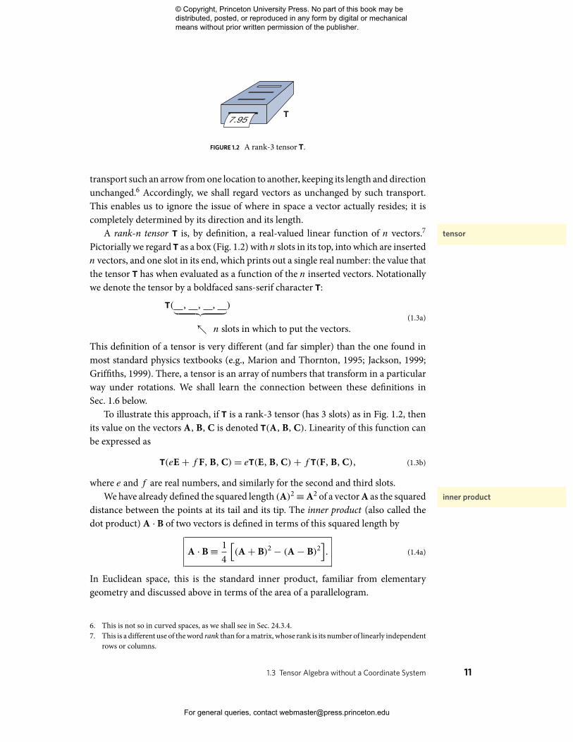
FIGURE 1.2 A rank-3 tensor T.

transport such an arrow from one location to another, keeping its length and directionunchanged.6 Accordingly, we shall regard vectors as unchanged by such transport.This enables us to ignore the issue of where in space a vector actually resides; it iscompletely determined by its direction and its length.

tensorA rank-n tensor T is, by definition, a real-valued linear function of n vectors.7

Pictorially we regard T as a box (Fig. 1.2) with n slots in its top, into which are insertedn vectors, and one slot in its end, which prints out a single real number: the value thatthe tensor T has when evaluated as a function of the n inserted vectors. Notationallywe denote the tensor by a boldfaced sans-serif character T:

T( , , ,︸︷︷︸)↖ n slots in which to put the vectors.

(1.3a)

This definition of a tensor is very different (and far simpler) than the one found inmost standard physics textbooks (e.g., Marion and Thornton, 1995; Jackson, 1999;Griffiths, 1999). There, a tensor is an array of numbers that transform in a particularway under rotations. We shall learn the connection between these definitions inSec. 1.6 below.

To illustrate this approach, if T is a rank-3 tensor (has 3 slots) as in Fig. 1.2, thenits value on the vectors A, B, C is denoted T(A, B, C). Linearity of this function canbe expressed as

T(eE + f F, B, C)= eT(E, B, C)+ f T(F, B, C), (1.3b)

where e and f are real numbers, and similarly for the second and third slots.inner productWe have already defined the squared length (A)2≡A2 of a vector A as the squared

distance between the points at its tail and its tip. The inner product (also called thedot product) A . B of two vectors is defined in terms of this squared length by

A . B≡ 14

[(A+ B)2 − (A− B)2

]. (1.4a)

In Euclidean space, this is the standard inner product, familiar from elementarygeometry and discussed above in terms of the area of a parallelogram.

6. This is not so in curved spaces, as we shall see in Sec. 24.3.4.7. This is a different use of the word rank than for a matrix, whose rank is its number of linearly independent

rows or columns.

1.3 Tensor Algebra without a Coordinate System 11



One can show that the inner product (1.4a) is a real-valued linear function of eachof its vectors. Therefore, we can regard it as a tensor of rank 2. When so regarded, theinner product is denoted g( , ) and is called the metric tensor. In other words, themetric tensor

metric tensor g is that linear function of two vectors whose value is given by

g(A, B)≡ A . B. (1.4b)

Notice that, because A . B= B . A, the metric tensor is symmetric in its two slots—one gets the same real number independently of the order in which one inserts thetwo vectors into the slots:

g(A, B)= g(B, A). (1.4c)

With the aid of the inner product, we can regard any vector A as a tensor of rankone: the real number that is produced when an arbitrary vector C is inserted into A’ssingle slot is

A(C)≡ A . C. (1.4d)

In Newtonian physics, we rarely meet tensors of rank higher than two. However,second-rank tensors appear frequently—often in roles where one sticks a single vectorinto the second slot and leaves the first slot empty, thereby producing a single-slottedentity, a vector. An example that we met in Sec. 1.1.1 is a rigid body’s moment-of-inertia tensor I( , ), which gives us the body’s angular momentum J( )= I( , �)when its angular velocity � is inserted into its second slot.8 Another example is thestress tensor of a solid, a fluid, a plasma, or a field (Sec. 1.9 below).

tensor product From three vectors A, B, C, we can construct a tensor, their tensor product (alsocalled outer product in contradistinction to the inner product A . B), defined asfollows:

A⊗ B⊗ C(E, F, G)≡ A(E)B(F)C(G)= (A . E)(B . F)(C . G). (1.5a)

Here the first expression is the notation for the value of the new tensor, A⊗ B⊗ Cevaluated on the three vectors E, F, G; the middle expression is the ordinary productof three real numbers, the value of A on E, the value of B on F, and the value of Con G; and the third expression is that same product with the three numbers rewrittenas scalar products. Similar definitions can be given (and should be obvious) for thetensor product of any number of vectors, and of any two or more tensors of any rank;for example, if T has rank 2 and S has rank 3, then

T⊗ S(E, F, G, H, J)≡ T(E, F)S(G, H, J). (1.5b)

One last geometric (i.e., frame-independent) concept we shall need is contraction.contraction

We illustrate this concept first by a simple example, then give the general definition.

8. Actually, it doesn’t matter which slot, since I is symmetric.




From two vectors A and B we can construct the tensor product A ⊗ B (a second-rank tensor), and we can also construct the scalar product A . B (a real number, i.e., ascalar, also known as a rank-0 tensor). The process of contraction is the constructionof A . B from A⊗ B:

contraction(A⊗ B)≡ A . B. (1.6a)

One can show fairly easily using component techniques (Sec. 1.5 below) that anysecond-rank tensor T can be expressed as a sum of tensor products of vectors, T =A⊗ B+ C⊗D+ . . . . Correspondingly, it is natural to define the contraction of T

to be contraction(T)=A . B+ C . D+ . . . . Note that this contraction process lowersthe rank of the tensor by two, from 2 to 0. Similarly, for a tensor of rank n one canconstruct a tensor of rank n − 2 by contraction, but in this case one must specifywhich slots are to be contracted. For example, if T is a third-rank tensor, expressibleas T= A⊗ B⊗ C+ E⊗ F⊗G+ . . ., then the contraction of T on its first and thirdslots is the rank-1 tensor (vector)

1&3contraction(A⊗ B⊗ C + E ⊗ F⊗ G+ . . .)≡ (A . C)B+ (E . G)F+ . . . .(1.6b)

Unfortunately, there is no simple index-free notation for contraction in common use.All the concepts developed in this section (vector, tensor, metric tensor, inner

product, tensor product, and contraction of a tensor) can be carried over, with nochange whatsoever, into any vector space9 that is endowed with a concept of squaredlength—for example, to the 4-dimensional spacetime of special relativity (nextchapter).

1.41.4 Particle Kinetics and Lorentz Force in Geometric Language

In this section, we illustrate our geometric viewpoint by formulating Newton’s lawsof motion for particles.

In Newtonian physics, a classical particle moves through Euclidean 3-space asuniversal time t passes. At time t it is located at some point x(t) (its position). The

trajectory, velocity,momentum, acceleration,and energy

function x(t) represents a curve in 3-space, the particle’s trajectory. The particle’svelocity v(t) is the time derivative of its position, its momentum p(t) is the product ofits mass m and velocity, its acceleration a(t) is the time derivative of its velocity, andits kinetic energy E(t) is half its mass times velocity squared:

v(t)= dxdt

, p(t)=mv(t), a(t)= dvdt= d

2xdt2

, E(t)= 12mv2. (1.7a)

9. Or, more precisely, any vector space over the real numbers. If the vector space’s scalars are complexnumbers, as in quantum mechanics, then slight changes are needed.

1.4 Particle Kinetics and Lorentz Force in Geometric Language 13



Since points in 3-space are geometric objects (defined independently of any coordi-nate system), so also are the trajectory x(t), the velocity, the momentum, the acceler-ation, and the energy. (Physically, of course, the velocity has an ambiguity; it dependson one’s standard of rest.)

Newton’s second law of motion states that the particle’s momentum can changeonly if a force F acts on it, and that its change is given by

dp/dt =ma = F. (1.7b)

If the force is produced by an electric field E and magnetic field B, then this law ofmotion in SI units takes the familiar Lorentz-force form

dp/dt = q(E + v × B). (1.7c)

(Here we have used the vector cross product, with which the reader should be familiar,and which will be discussed formally in Sec. 1.7.)

laws of motion The laws of motion (1.7) are geometric relationships among geometric objects.Let us illustrate this using something very familiar, planetary motion. Consider alight planet orbiting a heavy star. If there were no gravitational force, the planetwould continue in a straight line with constant velocity v and speed v = |v|, sweepingout area A at a rate dA/dt = rvt/2, where r is the radius, and vt is the tangentialspeed. Elementary geometry equates this to the constant vb/2, where b is the impactparameter—the smallest separation from the star. Now add a gravitational force F andlet it cause a small radial impulse. A second application of geometry showed Newtonthat the product rvt/2 is unchanged to first order in the impulse, and he recoveredKepler’s second law (dA/dt = const) without introducing coordinates.10

Contrast this approach with one relying on coordinates. For example, one in-troduces an (r , φ) coordinate system, constructs a lagrangian and observes that thecoordinate φ is ignorable; then the Euler-Lagrange equations immediately imply theconservation of angular momentum, which is equivalent to Kepler’s second law. So,which of these two approaches is preferable? The answer is surely “both!” Newtonwrote the Principia in the language of geometry at least partly for a reason that remainsvalid today: it brought him a quick understanding of fundamental laws of physics.Lagrange followed his coordinate-based path to the function that bears his name,because he wanted to solve problems in celestial mechanics that would not yield to

10. Continuing in this vein, when the force is inverse square, as it is for gravity and electrostatics, we canuse Kepler’s second law to argue that when the orbit turns through a succession of equal angles dθ ,its successive changes in velocity dv = adt (with a the gravitational acceleration) all have the samemagnitude |dv| and have the same angles dθ from one to another. So, if we trace the head of the velocityvector in velocity space, it follows a circle. The circle is not centered on zero velocity when the eccentricityis nonzero but there exists a reference frame in which the speed of the planet is constant. This graphicalrepresentation is known as a hodograph, and similar geometrical approaches are used in fluid mechanics.For Richard Feynman’s masterful presentation of these ideas to first-year undergraduates, see Goodsteinand Goodstein (1996).




Newton’s approach. So it is today. Geometry and analysis are both indispensible. In thedomain of classical physics, the geometry is of greater importance in deriving and un-derstanding fundamental laws and has arguably been underappreciated; coordinateshold sway when we apply these laws to solve real problems. Today, both old and newlaws of physics are commonly expressed geometrically, using lagrangians, hamiltoni-ans, and actions, for example Hamilton’s action principle δ

∫Ldt = 0 where L is the

coordinate-independent lagrangian. Indeed, being able to do this without introducingcoordinates is a powerful guide to deriving these laws and a tool for comprehendingtheir implications.

symmetry andconservation laws

A comment is needed on the famous connection between symmetry and conserva-tion laws.In our example above, angular momentum conservation followed from axialsymmetry which was embodied in the lagrangian’s independence of the angle φ; butwe also deduced it geometrically. This is usually the case in classical physics; typically,we do not need to introduce a specific coordinate system to understand symmetryand to express the associated conservation laws. However, symmetries are sometimeswell hidden, for example with a nutating top, and coordinate transformations are thenusually the best approach to uncover them.

Often in classical physics, real-world factors invalidate or complicate Lagrange’sand Hamilton’s coordinate-based analytical dynamics, and so one is driven to geo-metric considerations. As an example, consider a spherical marble rolling on a flathorizontal table. The analytical dynamics approach is to express the height of themarble’s center of mass and the angle of its rotation as constraints and align the basisvectors so there is a single horizontal coordinate defined by the initial condition. It isthen deduced that linear and angular momenta are conserved. Of course that resultis trivial and just as easily gotten without this formalism. However, this model is alsoused for many idealized problems where the outcome is far from obvious and the ap-proach is brilliantly effective. But consider the real world in which tables are warpedand bumpy, marbles are ellipsoidal and scratched, air imposes a resistance, and woodand glass comprise polymers that attract one another. And so on. When one includesthese factors, it is to geometry that one quickly turns to understand the real marble’sactual dynamics. Even ignoring these effects and just asking what happens when themarble rolls off the edge of a table introduces a nonholonomic constraint, and figuringout where it lands and how fast it is spinning are best addressed not by the methods ofLagrange and Hamilton, but instead by considering the geometry of the gravitationaland reaction forces. In the following chapters, we shall encounter many exampleswhere we have to deal with messy complications like these.

EXERCISESExercise 1.1 Practice: Energy Change for Charged ParticleWithout introducing any coordinates or basis vectors, show that when a particle withcharge q interacts with electric and magnetic fields, its kinetic energy changes at a rate

dE/dt = q v . E. (1.8)

1.4 Particle Kinetics and Lorentz Force in Geometric Language 15



Exercise 1.2 Practice: Particle Moving in a Circular OrbitConsider a particle moving in a circle with uniform speed v = |v| and uniformmagnitude a = |a| of acceleration. Without introducing any coordinates or basisvectors, do the following.

(a) At any moment of time, let n= v/v be the unit vector pointing along the velocity,and let s denote distance that the particle travels in its orbit. By drawing a picture,show that dn/ds is a unit vector that points to the center of the particle’s circularorbit, divided by the radius of the orbit.

(b) Show that the vector (not unit vector) pointing from the particle’s location to thecenter of its orbit is (v/a)2a.

1.5 1.5 Component Representation of Tensor Algebra

Cartesian coordinates andorthonormal basis vectors

In the Euclidean 3-space of Newtonian physics, there is a unique set of orthonormalbasis vectors {ex , ey , ez} ≡ {e1, e2, e3} associated with any Cartesian coordinate system{x , y , z} ≡ {x1, x2, x3} ≡ {x1, x2, x3}. (In Cartesian coordinates in Euclidean space,we usually place indices down, but occasionally we place them up. It doesn’t matter.By definition, in Cartesian coordinates a quantity is the same whether its index isdown or up.) The basis vector ej points along the xj coordinate direction, which isorthogonal to all the other coordinate directions, and it has unit length (Fig. 1.3), so

ej . ek = δjk , (1.9a)

where δjk is the Kronecker delta.Any vector A in 3-space can be expanded in terms of this basis:

A= Ajej . (1.9b)

Here and throughout this book, we adopt the Einstein summation convention: repeatedEinstein summationconvention indices (in this case j ) are to be summed (in this 3-space case over j = 1, 2, 3), unlessCartesian components of avector

otherwise instructed. By virtue of the orthonormality of the basis, the componentsAj of A can be computed as the scalar product

Aj = A . ej . (1.9c)

[The proof of this is straightforward: A . ej = (Akek) . ej = Ak(ek . ej ) = Akδkj =Aj .]

Any tensor, say, the third-rank tensor T( , , ), can be expanded in terms oftensor products of the basis vectors:

T = Tijkei ⊗ ej ⊗ ek . (1.9d)




x

y

z

e3

e2e1

FIGURE 1.3 The orthonormal basis vectorsej associated with a Euclidean coordi-nate system in Euclidean 3-space.

The components Tijk of T can be computed from T and the basis vectors by the Cartesian components of atensorgeneralization of Eq. (1.9c):

Tijk = T(ei , ej , ek). (1.9e)

[This equation can be derived using the orthonormality of the basis in the same wayas Eq. (1.9c) was derived.] As an important example, the components of the metrictensor are gjk = g(ej , ek)= ej . ek = δjk [where the first equality is the method (1.9e)of computing tensor components, the second is the definition (1.4b) of the metric, andthe third is the orthonormality relation (1.9a)]:

gjk = δjk . (1.9f)

The components of a tensor product [e.g., T( , , )⊗ S( , )] are easily de-duced by inserting the basis vectors into the slots [Eq. (1.9e)]; they are T(ei , ej , ek)⊗S(el , em)= TijkSlm [cf. Eq. (1.5a)]. In words, the components of a tensor product areequal to the ordinary arithmetic product of the components of the individual tensors.

In component notation, the inner product of two vectors and the value of a tensorwhen vectors are inserted into its slots are given by

A . B= AjBj , T(A, B, C)= TijkAiBjCk , (1.9g)

as one can easily show using previous equations. Finally, the contraction of a tensor[say, the fourth-rank tensor R( , , , )] on two of its slots (say, the first andthird) has components that are easily computed from the tensor’s own components:

components of [1&3contraction of R]= Rijik . (1.9h)

Note thatRijik is summed on the i index, so it has only two free indices, j and k, andthus is the component of a second-rank tensor, as it must be if it is to represent thecontraction of a fourth-rank tensor.

1.5.11.5.1 Slot-Naming Index Notation

We now pause in our development of the component version of tensor algebra tointroduce a very important new viewpoint.

1.5 Component Representation of Tensor Algebra 17



BOX 1.2. VECTORS AND TENSORS IN QUANTUM THEORY

The laws of quantum theory, like all other laws of Nature, can be expressed asgeometric relationships among geometric objects. Most of quantum theory’sgeometric objects, like those of classical theory, are vectors and tensors: thequantum state |ψ〉 of a physical system (e.g., a particle in a harmonic-oscillatorpotential) is a Hilbert-space vector—a generalization of a Euclidean-spacevector A. There is an inner product, denoted 〈φ|ψ〉, between any two states|φ〉 and |ψ〉, analogous to B . A; but B . A is a real number, whereas 〈φ|ψ〉 isa complex number (and we add and subtract quantum states with complex-number coefficients). The Hermitian operators that represent observables(e.g., the hamiltonian H for the particle in the potential) are two-slotted(second-rank), complex-valued functions of vectors; 〈φ|H |ψ〉 is the complexnumber that one gets when one inserts φ and ψ into the first and secondslots of H . Just as, in Euclidean space, we get a new vector (first-rank tensor)T( , A) when we insert the vector A into the second slot of T, so in quantumtheory we get a new vector (physical state) H |ψ〉 (the result of letting H “acton” |ψ〉) when we insert |ψ〉 into the second slot of H . In these senses, we canregard T as a linear map of Euclidean vectors into Euclidean vectors and H asa linear map of states (Hilbert-space vectors) into states.

For the electron in the hydrogen atom, we can introduce a set oforthonormal basis vectors {|1〉, |2〉, |3〉, . . .}, that is, the atom’s energyeigenstates, with 〈m|n〉 = δmn. But by contrast with Newtonian physics,where we only need three basis vectors (because our Euclidean space is 3-dimensional), for the particle in a harmonic-oscillator potential, we need aninfinite number of basis vectors (since the Hilbert space of all states is infinite-dimensional). In the particle’s quantum-state basis, any observable (e.g., theparticle’s position x or momentum p) has components computed by insertingthe basis vectors into its two slots: xmn = 〈m|x|n〉, and pmn = 〈m|p|n〉. In thisbasis, the operator xp (which maps states into states) has components xjkpkm(a matrix product), and the noncommutation of position and momentum[x , p]= i� (an important physical law) is expressible in terms of componentsas xjkpkm − pjkxkm = i�δjm.

Consider the rank-2 tensor F( , ). We can define a new tensor G( , ) to bethe same as F, but with the slots interchanged: i.e., for any two vectors A and B, it istrue that G(A, B)= F(B, A). We need a simple, compact way to indicate that F andG are equal except for an interchange of slots. The best way is to give the slots names,say a and b—i.e., to rewrite F( , ) as F( a , b) or more conveniently as Fab, andthen to write the relationship between G and F as Gab = Fba. “NO!” some readers




might object. This notation is indistinguishable from our notation for components ona particular basis. “GOOD!” a more astute reader will exclaim. The relationGab = Fbain a particular basis is a true statement if and only if “G= F with slots interchanged”is true, so why not use the same notation to symbolize both? In fact, we shall dothis. We ask our readers to look at any “index equation,” such asGab = Fba, like theywould look at an Escher drawing: momentarily think of it as a relationship betweencomponents of tensors in a specific basis; then do a quick mind-flip and regard it quitedifferently, as a relationship between geometric, basis-independent tensors with theindices playing the roles of slot names. This mind-flip approach to tensor algebra willpay substantial dividends.

slot-naming index notationAs an example of the power of this slot-naming index notation, consider the con-traction of the first and third slots of a third-rank tensor T. In any basis the componentsof 1&3contraction(T) are Taba; cf. Eq. (1.9h). Correspondingly, in slot-naming indexnotation we denote 1&3contraction(T) by the simple expression Taba. We can thinkof the first and third slots as annihilating each other by the contraction, leaving freeonly the second slot (named b) and therefore producing a rank-1 tensor (a vector).

We should caution that the phrase “slot-naming index notation” is unconventional.You are unlikely to find it in any other textbooks. However, we like it. It says preciselywhat we want it to say.

1.5.21.5.2 Particle Kinetics in Index Notation

As an example of slot-naming index notation, we can rewrite the equations of particlekinetics (1.7) as follows:

vi = dxidt

, pi =mvi , ai = dvidt= d

2xidt2

,

E = 12mvjvj , dpi

dt= q(Ei + εijkvjBk). (1.10)

(In the last equation εijk is the so-called Levi-Civita tensor, which is used to producethe cross product; we shall learn about it in Sec. 1.7. And note that the scalar energyE must not be confused with the electric field vector Ei.)

Equations (1.10) can be viewed in either of two ways: (i) as the basis-independentgeometric laws v = dx/dt , p=mv, a = dv/dt = d2x/dt2, E = 1

2mv2, and dp/dt =q(E + v × B) written in slot-naming index notation; or (ii) as equations for thecomponents of v, p, a, E, and B in some particular Cartesian coordinate system.

EXERCISESExercise 1.3 Derivation: Component Manipulation RulesDerive the component manipulation rules (1.9g) and (1.9h).

Exercise 1.4 Example and Practice: Numerics of Component ManipulationsThe third-rank tensor S( , , ) and vectors A and B have as their only nonzerocomponents S123 = S231 = S312 = +1, A1 = 3, B1 = 4, B2 = 5. What are the

1.5 Component Representation of Tensor Algebra 19



components of the vector C= S(A, B, ), the vector D= S(A, , B), and the tensorW = A⊗ B?

[Partial solution: In component notation, Ck = SijkAiBj , where (of course) wesum over the repeated indices i and j . This tells us that C1= S231A2B3, becauseS231 is the only component of S whose last index is a 1; this in turn implies thatC1= 0, since A2 = 0. Similarly, C2 = S312A3B1= 0 (because A3= 0). Finally, C3=S123A1B2 =+1× 3× 5= 15. Also, in component notation Wij = AiBj , so W11=A1× B1= 3× 4 = 12, and W12 = A1× B2 = 3× 5= 15. Here the × stands fornumerical multiplication, not the vector cross product.]

Exercise 1.5 Practice: Meaning of Slot-Naming Index Notation(a) The following expressions and equations are written in slot-naming index nota-

tion. Convert them to geometric, index-free notation:AiBjk,AiBji, Sijk = Skji,AiBi = AiBjgij .

(b) The following expressions are written in geometric, index-free notation. Convertthem to slot-naming index notation: T( , , A), T( , S(B, ), ).

1.6 1.6 Orthogonal Transformations of Bases

Consider two different Cartesian coordinate systems {x , y , z} ≡ {x1, x2, x3}, and{x , y , z} ≡ {x1, x2, x3}. Denote by {ei} and {ep} the corresponding bases. It is possibleto expand the basis vectors of one basis in terms of those of the other. We denote theexpansion coefficients by the letter R and write

ei = epRpi , ep = eiRip. (1.11)

The quantities Rpi and Rip are not the components of a tensor; rather, they are theelements of transformation matrices

[Rpi]=⎡⎢⎣ R11 R12 R13

R21 R22 R23

R31 R32 R33

⎤⎥⎦, [Rip]=⎡⎢⎣ R11 R12 R13

R21 R22 R23

R31 R32 R33

⎤⎥⎦. (1.12a)

(Here and throughout this book we use square brackets to denote matrices.) Thesetwo matrices must be the inverse of each other, since one takes us from the barred basisto the unbarred, and the other in the reverse direction, from unbarred to barred:

RpiRiq = δpq , RipRpj = δij . (1.12b)

The orthonormality requirement for the two bases implies that δij = ei . ej =(epRpi) . (eqRqj) = RpiRqj(ep . eq) = RpiRqjδpq = RpiRpj. This says that thetranspose of [Rpi] is its inverse—which we have already denoted by [Rip]:

[Rip]≡ inverse([Rpi])= transpose

([Rpi]). (1.12c)




This property implies that the transformation matrix is orthogonal, so the transfor- orthogonal transformationand rotationmation is a reflection or a rotation (see, e.g., Goldstein, Poole, and Safko, 2002). Thus

(as should be obvious and familiar), the bases associated with any two Euclidean co-ordinate systems are related by a reflection or rotation, and the matrices (1.12a) arecalled rotation matrices. Note that Eq. (1.12c) does not say that [Rip] is a symmetricmatrix. In fact, most rotation matrices are not symmetric [see, e.g., Eq. (1.14)].

The fact that a vector A is a geometric, basis-independent object implies thatA= Aiei = Ai(epRpi)= (RpiAi)ep = Apep:

Ap = RpiAi , and similarly, Ai = RipAp; (1.13a)

and correspondingly for the components of a tensor:

Tpqr = RpiRqjRrkTijk , Tijk = RipRjqRkrTpqr . (1.13b)

It is instructive to compare the transformation law (1.13a) for the components ofa vector with Eqs. (1.11) for the bases. To make these laws look natural, we haveplaced the transformation matrix on the left in the former and on the right in thelatter. In Minkowski spacetime (Chap. 2), the placement of indices, up or down, willautomatically tell us the order.

If we choose the origins of our two coordinate systems to coincide, then the vectorx reaching from the common origin to some point P, whose coordinates arexj andxp,has components equal to those coordinates; and as a result, the coordinates themselvesobey the same transformation law as any other vector:

xp = Rpixi , xi = Ripxp . (1.13c)

The product of two rotation matrices [RipRp ¯s] is another rotation matrix [Ri ¯s],which transforms the Cartesian bases e ¯s to ei. Under this product rule, the rotation

rotation groupmatrices form a mathematical group: the rotation group, whose group representationsplay an important role in quantum theory.

EXERCISESExercise 1.6 **Example and Practice: Rotation in x-y PlaneConsider two Cartesian coordinate systems rotated with respect to each other in thex-y plane as shown in Fig. 1.4.(a) Show that the rotation matrix that takes the barred basis vectors to the unbarred

basis vectors is

[Rpi]=⎡⎢⎣ cos φ sin φ 0− sin φ cos φ 0

0 0 1

⎤⎥⎦, (1.14)

and show that the inverse of this rotation matrix is, indeed, its transpose, as itmust be if this is to represent a rotation.

(b) Verify that the two coordinate systems are related by Eq. (1.13c).

1.6 Orthogonal Transformations of Bases 21



x

yy

x

eyex

φ

ex

ey

FIGURE 1.4 Two Cartesian coordinate systems {x , y , z} and{x , y , z} and their basis vectors in Euclidean space, rotatedby an angle φ relative to each other in the x-y plane. The z- andz-axes point out of the paper or screen and are not shown.

(c) Let Aj be the components of the electromagnetic vector potential that lies inthe x-y plane, so that Az = 0. The two nonzero components Ax and Ay can beregarded as describing the two polarizations of an electromagnetic wave propa-gating in the z direction. Show thatAx + iAy = (Ax + iAy)e−iφ. One can show(cf. Sec. 27.3.3) that the factor e−iφ implies that the quantum particle associ-ated with the wave—the photon—has spin one [i.e., spin angular momentum� = (Planck’s constant)/2π].

(d) Let hjk be the components of a symmetric tensor that is trace-free (its contractionhjj vanishes) and is confined to the x-y plane (so hzk = hkz = 0 for all k). Thenthe only nonzero components of this tensor are hxx = −hyy and hxy = hyx.As we shall see in Sec. 27.3.1, this tensor can be regarded as describing thetwo polarizations of a gravitational wave propagating in the z direction. Showthat hxx + ihxy = (hxx + ihxy)e−2iφ. The factor e−2iφ implies that the quantumparticle associated with the gravitational wave (the graviton) has spin two (spinangular momentum 2�); cf. Eq. (27.31) and Sec. 27.3.3.

1.7 1.7 Differentiation of Scalars, Vectors, and Tensors; Cross Product and Curl

Consider a tensor field T(P) in Euclidean 3-space and a vector A. We define thedirectional derivative directional derivative of T along A by the obvious limiting procedure

∇AT ≡ limε→0

1ε

[T(xP + εA)− T(xP)] (1.15a)

and similarly for the directional derivative of a vector field B(P) and a scalar fieldψ(P). [Here we have denoted points, e.g., P, by the vector xP that reaches from some




arbitrary origin to the point, and T(xP) denotes the field’s dependence on location inspace; T’s slots and dependence on what goes into the slots are suppressed; and theunits of ε are chosen to ensure that εA has the same units as xP . There is no otherappearance of vectors in this chapter.] In definition (1.15a), the quantity in squarebrackets is simply the difference between two linear functions of vectors (two tensors),so the quantity on the left-hand side is also a tensor with the same rank as T.

It should not be hard to convince oneself that this directional derivative∇AT of anytensor field T is linear in the vector A along which one differentiates. Correspondingly,if T has rankn (n slots), then there is another tensor field, denoted∇T, with rankn+ 1,such that

∇AT =∇T( , , , A). (1.15b)

Here on the right-hand side the first n slots (3 in the case shown) are left empty, and gradientA is put into the last slot (the “differentiation slot”). The quantity ∇T is called thegradient of T. In slot-naming index notation, it is conventional to denote this gradientby Tabc;d , where in general the number of indices preceding the semicolon is the rankof T. Using this notation, the directional derivative of T along A reads [cf. Eq. (1.15b)]Tabc;jAj .

It is not hard to show that in any Cartesian coordinate system, the components ofthe gradient are nothing but the partial derivatives of the components of the originaltensor, which we denote by a comma:

Tabc;j = ∂Tabc∂xj

≡ Tabc ,j . (1.15c)

In a non-Cartesian basis (e.g., the spherical and cylindrical bases often used in electro-magnetic theory), the components of the gradient typically are not obtained by simplepartial differentiation [Eq. (1.15c) fails] because of turning and/or length changes ofthe basis vectors as we go from one location to another. In Sec. 11.8, we shall learnhow to deal with this by using objects called connection coefficients. Until then, weconfine ourselves to Cartesian bases, so subscript semicolons and subscript commas(partial derivatives) can be used interchangeably.

Because the gradient and the directional derivative are defined by the same stan-dard limiting process as one uses when defining elementary derivatives, they obey thestandard (Leibniz) rule for differentiating products:

∇A(S⊗ T = (∇AS)⊗ T + S⊗∇AT,or (SabTcde);jAj = (Sab;jAj)Tcde + Sab(Tcde;jAj); (1.16a)

and

∇A(f T)= (∇Af )T + f∇AT, or (f Tabc);jAj = (f;jAj)Tabc + f Tabc;jAj .

(1.16b)

1.7 Differentiation of Scalars, Vectors, and Tensors; Cross Product and Curl 23



In an orthonormal basis these relations should be obvious: they follow from theLeibniz rule for partial derivatives.

Because the components gab of the metric tensor are constant in any Cartesiancoordinate system, Eq. (1.15c) (which is valid in such coordinates) guarantees thatgab;j = 0; i.e., the metric has vanishing gradient:

∇g= 0, or gab;j = 0. (1.17)

From the gradient of any vector or tensor we can construct several other importantderivatives by contracting on slots:

1. Since the gradient ∇A of a vector field A has two slots, ∇A( , ), we cancontract its slots on each other to obtain a scalar field. That scalar field is the

divergence divergence of A and is denoted

∇ . A≡ (contraction of ∇A)= Aa ;a . (1.18)

2. Similarly, if T is a tensor field of rank 3, then Tabc;c is its divergence on itsthird slot, and Tabc;b is its divergence on its second slot.

3. By taking the double gradient and then contracting on the two gradient slotswe obtain, from any tensor field T, a new tensor field with the same rank,

laplacian ∇2T ≡ (∇ . ∇)T , or Tabc;jj . (1.19)

Here and henceforth, all indices following a semicolon (or comma) representgradients (or partial derivatives):Tabc;jj ≡ Tabc;j ;j ,Tabc ,jk ≡ ∂2Tabc/∂xj∂xk.The operator ∇2 is called the laplacian.

The metric tensor is a fundamental property of the space in which it lives; itembodies the inner product and hence the space’s notion of distance. In addition tothe metric, there is one (and only one) other fundamental tensor that describes a pieceof Euclidean space’s geometry: the Levi-Civita tensor ε, which embodies the space’sLevi-Civita tensor

notion of volume.In a Euclidean space with dimension n, the Levi-Civita tensor ε is a completely

antisymmetric tensor with rank n (with n slots). A parallelepiped whose edges are then vectors A, B, . . . , F is said to have the volume

volume volume= ε(A, B, . . . , F). (1.20)

(We justify this definition in Sec. 1.8.) Notice that this volume can be positive ornegative, and if we exchange the order of the parallelepiped’s legs, the volume’s signchanges: ε(B, A, . . . , F)=−ε(A, B, . . . , F) by antisymmetry of ε.

It is easy to see (Ex. 1.7) that (i) the volume vanishes unless the legs are all linearlyindependent, (ii) once the volume has been specified for one parallelepiped (oneset of linearly independent legs), it is thereby determined for all parallelepipeds,and therefore, (iii) we require only one number plus antisymmetry to determine ε




fully. If the chosen parallelepiped has legs that are orthonormal (all are orthogonalto one another and all have unit length—properties determined by the metric g),then it must have unit volume, or more precisely volume ±1. This is a compatibilityrelation between g and ε. It is easy to see (Ex. 1.7) that (iv) ε is fully determined by itsantisymmetry, compatibility with the metric, and a single sign: the choice of whichparallelepipeds have positive volume and which have negative. It is conventionalin Euclidean 3-space to give right-handed parallelepipeds positive volume and left-handed ones negative volume: ε(A, B, C) is positive if, when we place our right thumbalong C and the fingers of our right hand along A, then bend our fingers, they sweeptoward B and not−B.

These considerations dictate that in a right-handed orthonormal basis of Eu-clidean 3-space, the only nonzero components of ε are

ε123=+1,

εabc =

⎧⎪⎨⎪⎩+1 if a , b, c is an even permutation of 1, 2, 3−1 if a , b, c is an odd permutation of 1, 2, 30 if a , b, c are not all different;

(1.21)

and in a left-handed orthonormal basis, the signs of these components are reversed.cross product and curlThe Levi-Civita tensor is used to define the cross product and the curl:

A× B≡ ε( , A, B); in slot-naming index notation, εijkAjBk; (1.22a)

∇× A≡ (the vector field whose slot-naming index form is εijkAk;j ). (1.22b)

[Equation (1.22b) is an example of an expression that is complicated if stated in index-free notation; it says that ∇×A is the double contraction of the rank-5 tensor ε⊗∇Aon its second and fifth slots, and on its third and fourth slots.]

Although Eqs. (1.22a) and (1.22b) look like complicated ways to deal with conceptsthat most readers regard as familiar and elementary, they have great power. The powercomes from the following property of the Levi-Civita tensor in Euclidean 3-space[readily derivable from its components (1.21)]:

εijmεklm = δijkl ≡ δikδjl − δil δjk . (1.23)

Here δik

is the Kronecker delta. Examine the 4-index delta function δijkl carefully; it saysthat either the indices above and below each other must be the same (i = k and j = l)with a+ sign, or the diagonally related indices must be the same (i = l and j = k) witha− sign. [We have put the indices ij of δijkl up solely to facilitate remembering this rule.Recall (first paragraph of Sec. 1.5) that in Euclidean space and Cartesian coordinates,it does not matter whether indices are up or down.] With the aid of Eq. (1.23) and theindex-notation expressions for the cross product and curl, one can quickly and easilyderive a wide variety of useful vector identities; see the very important Ex. 1.8.

1.7 Differentiation of Scalars, Vectors, and Tensors; Cross Product and Curl 25



EXERCISES Exercise 1.7 Derivation: Properties of the Levi-Civita TensorFrom its complete antisymmetry, derive the four properties of the Levi-Civita tensor,in n-dimensional Euclidean space, that are claimed in the text following Eq. (1.20).

Exercise 1.8 **Example and Practice: Vectorial Identities for the Cross Productand CurlHere is an example of how to use index notation to derive a vector identity for the dou-ble cross product A× (B× C): in index notation this quantity is εijkAj(εklmBlCm).By permuting the indices on the second ε and then invoking Eq. (1.23), we can writethis as εijkεlmkAjBlCm = δlmij AjBlCm. By then invoking the meaning of the 4-indexdelta function [Eq. (1.23)], we bring this into the form AjBiCj − AjBjCi, whichis the slot-naming index-notation form of (A . C)B− (A . B)C. Thus, it must be thatA× (B× C)= (A . C)B− (A . B)C. Use similar techniques to evaluate the followingquantities.

(a) ∇× (∇× A).(b) (A× B) . (C×D).(c) (A× B)× (C×D).

Exercise 1.9 **Example and Practice: Levi-Civita Tensor in 2-DimensionalEuclidean SpaceIn Euclidean 2-space, let {e1, e2} be an orthonormal basis with positive volume.

(a) Show that the components of ε in this basis are

ε12 =+1, ε21=−1, ε11= ε22 = 0. (1.24a)

(b) Show that

εikεjk = δij . (1.24b)

1.8 1.8 Volumes, Integration, and Integral Conservation Laws

In Cartesian coordinates of 2-dimensional Euclidean space, the basis vectors areorthonormal, so (with a conventional choice of sign) the components of the Levi-Civita tensor are given by Eqs. (1.24a). Correspondingly, the area (i.e., 2-dimensionalvolume) of a parallelogram whose sides are A and B is

2-volume= ε(A, B)= εabAaBb = A1B2 − A2B1= det[A1 B1

A2 B2

], (1.25)

a relation that should be familiar from elementary geometry. Equally familiar shouldbe the following expression for the 3-dimensional volume of a parallelepiped with legs




A, B, and C [which follows from the components (1.21) of the Levi-Civita tensor]:

3-volume3-volume= ε(A, B, C)= εijkAiBjCk =A . (B×C)= det

⎡⎢⎣ A1 B1 C1

A2 B2 C2

A3 B3 C3

⎤⎥⎦. (1.26)

Our formal definition (1.20) of volume is justified because it gives rise to these familiarequations.

Equations (1.25) and (1.26) are foundations from which one can derive the usualformulas dA = dx dy and dV = dx dy dz for the area and volume of elementarysurface and volume elements with Cartesian side lengths dx, dy, and dz (Ex. 1.10).

In Euclidean 3-space, we define the vectorial surface area of a 2-dimensionalparallelogram with legs A and B to be

�= A× B= ε( , A, B). (1.27)

This vectorial surface area has a magnitude equal to the area of the parallelogram vectorial surface areaand a direction perpendicular to it. Notice that this surface area ε( , A, B) can bethought of as an object that is waiting for us to insert a third leg, C, so as to computea 3-volume ε(C, A, B)—the volume of the parallelepiped with legs C, A, and B.

A parallelogram’s surface has two faces (two sides), called the positive face and thenegative face. If the vector C sticks out of the positive face, then �(C)= ε(C, A, B) ispositive; if C sticks out of the negative face, then �(C) is negative.

1.8.11.8.1 Gauss’s and Stokes’ Theorems

Such vectorial surface areas are the foundation for surface integrals in 3-dimensional Gauss’s and Stokes’theoremsspace and for the familiar Gauss’s theorem,∫

V3

(∇ . A)dV =∫∂V3

A . d� (1.28a)

(where V3 is a compact 3-dimensional region, and ∂V3 is its closed 2-dimensionalboundary) and Stokes’ theorem,∫

V2

∇× A . d�=∫∂V2

A . dl (1.28b)

(where V2 is a compact 2-dimensional region, ∂V2 is the 1-dimensional closed curvethat bounds it, and the last integral is a line integral around that curve); see, e.g.,Arfken, Weber, and Harris (2013).

This mathematics is illustrated by the integral and differential conservation lawsfor electric charge and for particles: The total charge and the total number of particlesinside a 3-dimensional region of space V3 are

∫V3ρe dV and

∫V3ndV , where ρe is

the charge density and n the number density of particles. The rates that charge andparticles flow out of V3 are the integrals of the current density j and the particle flux

1.8 Volumes, Integration, and Integral Conservation Laws 27



vector S over its boundary ∂V3. Therefore, the integral laws of charge conservation and

integral conservation laws

particle conservation are

d

dt

∫V3

ρe dV +∫∂V3

j . d�= 0, d

dt

∫V3

ndV +∫∂V3

S . d�= 0. (1.29)

Pull the time derivative inside each volume integral (where it becomes a partialderivative), and apply Gauss’s law to each surface integral; the results are

∫V3(∂ρe/∂t +

∇ . j)dV = 0 and similarly for particles. The only way these equations can be true forall choices of V3 is for the integrands to vanish:

∂ρe/∂t +∇ . j= 0, ∂n/∂t +∇ . S= 0. (1.30)

These are the differential conservation laws for charge and for particles. They have a

differential conservationlaws

standard, universal form: the time derivative of the density of a quantity plus thedivergence of its flux vanishes.

Note that the integral conservation laws (1.29) and the differential conservationlaws (1.30) require no coordinate system or basis for their description, and no coordi-nate system or basis was used in deriving the differential laws from the integral laws.This is an example of the fundamental principle that the Newtonian physical laws areall expressible as geometric relationships among geometric objects.

EXERCISES Exercise 1.10 Derivation and Practice: Volume Elements in Cartesian CoordinatesUse Eqs. (1.25) and (1.26) to derive the usual formulas dA= dxdy and dV = dxdydzfor the 2-dimensional and 3-dimensional integration elements, respectively, in right-handed Cartesian coordinates. [Hint: Use as the edges of the integration volumesdx ex, dy ey, and dz ez.]

Exercise 1.11 Example and Practice: Integral of a Vector Field over a SphereIntegrate the vector field A = zez over a sphere with radius a, centered at the originof the Cartesian coordinate system (i.e., compute

∫A . d�). Hints:

(a) Introduce spherical polar coordinates on the sphere, and construct the vectorialintegration element d� from the two legs adθ e

θand a sin θdφ e

φ. Here e

θand

eφ

are unit-length vectors along the θ and φ directions. (Here as in Sec. 1.6 andthroughout this book, we use accents on indices to indicate which basis the indexis associated with: hats here for the spherical orthonormal basis, bars in Sec. 1.6for the barred Cartesian basis.) Explain the factors adθ and a sin θdφ in thedefinitions of the legs. Show that

d�= ε( , eθ

, eφ)a2 sin θdθdφ . (1.31)

(b) Using z= a cos θ and ez = cos θer − sin θeθ

on the sphere (where er is the unitvector pointing in the radial direction), show that

A . d�= a cos2 θ ε(er , eθ

, eφ) a2 sin θdθdφ .




(c) Explain why ε(er , eθ

, eφ)= 1.

(d) Perform the integral∫

A . d�over the sphere’s surface to obtain your final answer(4π/3)a3. This, of course, is the volume of the sphere. Explain pictorially why thishad to be the answer.

Exercise 1.12 Example: Faraday’s Law of InductionOne of Maxwell’s equations says that ∇× E =−∂B/∂t (in SI units), where E andB are the electric and magnetic fields. This is a geometric relationship between ge-ometric objects; it requires no coordinates or basis for its statement. By integratingthis equation over a 2-dimensional surface V2 with boundary curve ∂V2 and applyingStokes’ theorem, derive Faraday’s law of induction—again, a geometric relationshipbetween geometric objects.

1.91.9 The Stress Tensor and Momentum Conservation

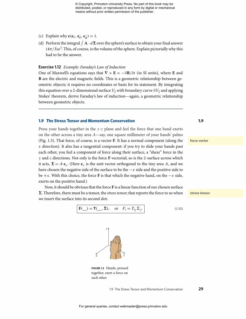
Press your hands together in the y-z plane and feel the force that one hand exertson the other across a tiny area A—say, one square millimeter of your hands’ palms

force vector(Fig. 1.5). That force, of course, is a vector F. It has a normal component (along thex direction). It also has a tangential component: if you try to slide your hands pasteach other, you feel a component of force along their surface, a “shear” force in they and z directions. Not only is the force F vectorial; so is the 2-surface across whichit acts, �= A ex. (Here ex is the unit vector orthogonal to the tiny area A, and wehave chosen the negative side of the surface to be the−x side and the positive side tobe +x. With this choice, the force F is that which the negative hand, on the −x side,exerts on the positive hand.)

Now, it should be obvious that the force F is a linear function of our chosen surfacestress tensor�. Therefore, there must be a tensor, the stress tensor, that reports the force to us when

we insert the surface into its second slot:

F( )= T( , �), or Fi = Tij�j . (1.32)

x y

z

FIGURE 1.5 Hands, pressedtogether, exert a force oneach other.

1.9 The Stress Tensor and Momentum Conservation 29



Newton’s law of action and reaction tells us that the force that the positive handexerts on the negative hand must be equal and opposite to that which the negativehand exerts on the positive. This shows up trivially in Eq. (1.32): by changing the signof �, one reverses which hand is regarded as negative and which positive, and sinceT is linear in �, one also reverses the sign of the force.

The definition (1.32) of the stress tensor gives rise to the following physical mean-ing of its components:

meaning of components ofstress tensor

Tjk =(j component of force per unit areaacross a surface perpendicular to ek

)

=⎛⎝ j component of momentum that crosses a unit

area that is perpendicular to ek, per unit time,with the crossing being from−xk to+xk

⎞⎠.(1.33)

The stresses inside a table with a heavy weight on it are described by the stresstensor T, as are the stresses in a flowing fluid or plasma, in the electromagnetic field,and in any other physical medium. Accordingly, we shall use the stress tensor as animportant mathematical tool in our study of force balance in kinetic theory (Chap.3), elasticity (Part IV), fluid dynamics (Part V), and plasma physics (Part VI).

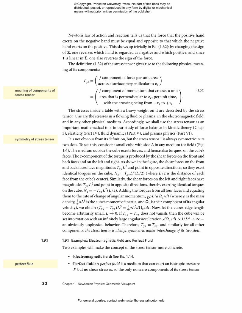
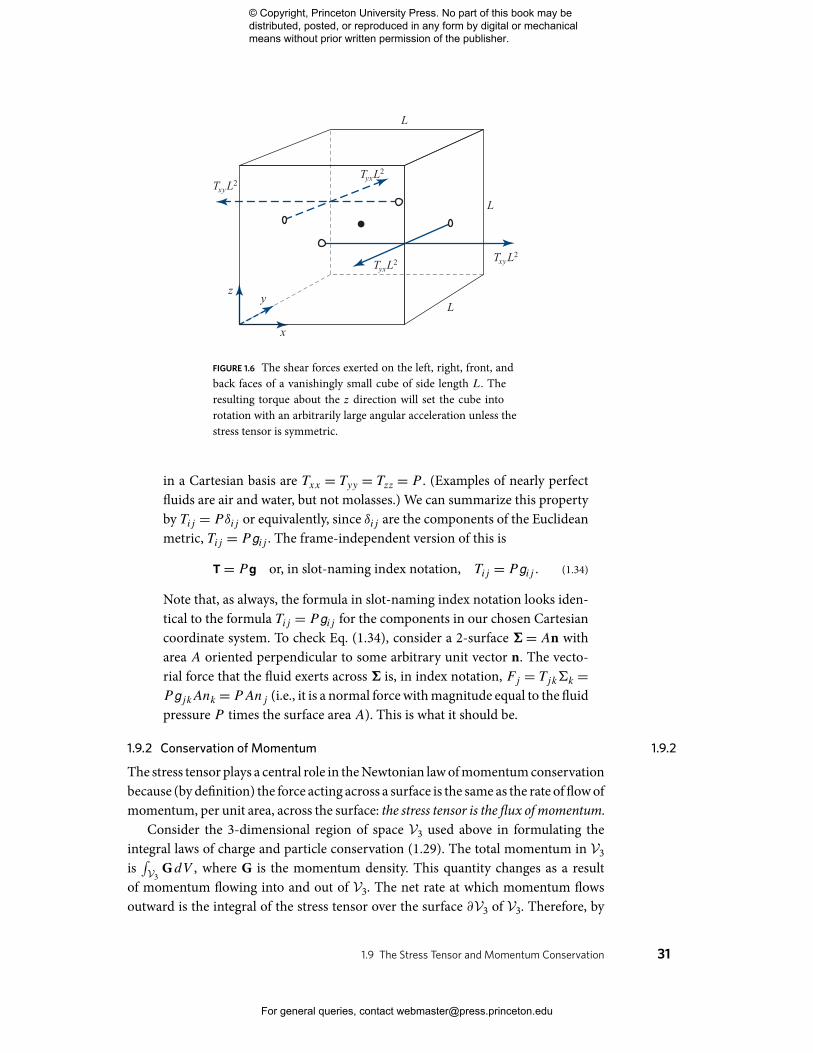
symmetry of stress tensor It is not obvious from its definition, but the stress tensor T is always symmetric in itstwo slots. To see this, consider a small cube with sideL in any medium (or field) (Fig.1.6). The medium outside the cube exerts forces, and hence also torques, on the cube’sfaces. The z-component of the torque is produced by the shear forces on the front andback faces and on the left and right. As shown in the figure, the shear forces on the frontand back faces have magnitudes TxyL2 and point in opposite directions, so they exertidentical torques on the cube, Nz = TxyL2(L/2) (where L/2 is the distance of eachface from the cube’s center). Similarly, the shear forces on the left and right faces havemagnitudesTyxL2 and point in opposite directions, thereby exerting identical torqueson the cube,Nz =−TyxL2(L/2). Adding the torques from all four faces and equatingthem to the rate of change of angular momentum, 1

6ρL5d�z/dt (where ρ is the mass

density, 16ρL

5 is the cube’s moment of inertia, and�z is the z component of its angularvelocity), we obtain (Txy − Tyx)L3= 1

6ρL5d�z/dt . Now, let the cube’s edge length

become arbitrarily small, L→ 0. If Txy − Tyx does not vanish, then the cube will beset into rotation with an infinitely large angular acceleration, d�z/dt ∝ 1/L2→∞—an obviously unphysical behavior. Therefore, Tyx = Txy, and similarly for all othercomponents: the stress tensor is always symmetric under interchange of its two slots.

1.9.1 1.9.1 Examples: Electromagnetic Field and Perfect Fluid

Two examples will make the concept of the stress tensor more concrete.

. Electromagnetic field: See Ex. 1.14.perfect fluid . Perfect fluid: A perfect fluid is a medium that can exert an isotropic pressure

P but no shear stresses, so the only nonzero components of its stress tensor




zy

x

L

L

L

TxyL2

TxyL2

TyxL2

TyxL2

FIGURE 1.6 The shear forces exerted on the left, right, front, andback faces of a vanishingly small cube of side length L. Theresulting torque about the z direction will set the cube intorotation with an arbitrarily large angular acceleration unless thestress tensor is symmetric.

in a Cartesian basis are Txx = Tyy = Tzz = P . (Examples of nearly perfectfluids are air and water, but not molasses.) We can summarize this propertyby Tij = Pδij or equivalently, since δij are the components of the Euclideanmetric, Tij = P gij . The frame-independent version of this is

T = Pg or, in slot-naming index notation, Tij = P gij . (1.34)

Note that, as always, the formula in slot-naming index notation looks iden-tical to the formula Tij = P gij for the components in our chosen Cartesiancoordinate system. To check Eq. (1.34), consider a 2-surface �= An witharea A oriented perpendicular to some arbitrary unit vector n. The vecto-rial force that the fluid exerts across � is, in index notation, Fj = Tjk�k =P gjkAnk = PAnj (i.e., it is a normal force with magnitude equal to the fluidpressure P times the surface area A). This is what it should be.

1.9.21.9.2 Conservation of Momentum

The stress tensor plays a central role in the Newtonian law of momentum conservationbecause (by definition) the force acting across a surface is the same as the rate of flow ofmomentum, per unit area, across the surface: the stress tensor is the flux of momentum.

Consider the 3-dimensional region of space V3 used above in formulating theintegral laws of charge and particle conservation (1.29). The total momentum in V3is∫V3

GdV , where G is the momentum density. This quantity changes as a resultof momentum flowing into and out of V3. The net rate at which momentum flowsoutward is the integral of the stress tensor over the surface ∂V3 of V3. Therefore, by

1.9 The Stress Tensor and Momentum Conservation 31



analogy with charge and particle conservation (1.29), the integral law of momentumconservation says

integral conservation ofmomentum

d

dt

∫V3

GdV +∫∂V3

T . d�= 0. (1.35)

By pulling the time derivative inside the volume integral (where it becomes apartial derivative) and applying the vectorial version of Gauss’s law to the surfaceintegral, we obtain

∫V3(∂G/∂t + ∇ . T) dV = 0. This can be true for all choices of

V3 only if the integrand vanishes:

∂G∂t+∇ . T = 0, or

∂Gj

∂t+ Tjk; k = 0. (1.36)

(Because T is symmetric, it does not matter which of its slots the divergence acts on.)This is the differential law of momentum conservation. It has the standard form for

differential conservationof momentum

any local conservation law: the time derivative of the density of some quantity (heremomentum), plus the divergence of the flux of that quantity (here the momentumflux is the stress tensor), is zero. We shall make extensive use of this Newtonian lawof momentum conservation in Part IV (elasticity), Part V (fluid dynamics), and PartVI (plasma physics).

EXERCISES Exercise 1.13 **Example: Equations of Motion for a Perfect Fluid(a) Consider a perfect fluid with density ρ, pressure P , and velocity v that vary in

time and space. Explain why the fluid’s momentum density is G= ρv, and explainwhy its momentum flux (stress tensor) is

T = Pg+ ρv ⊗ v , or, in slot-naming index notation, Tij = P gij + ρvivj .

(1.37a)

(b) Explain why the law of mass conservation for this fluid is

∂ρ

∂t+∇ . (ρv)= 0. (1.37b)

(c) Explain why the derivative operator

d

dt≡ ∂

∂t+ v . ∇ (1.37c)

describes the rate of change as measured by somebody who moves locally withthe fluid (i.e., with velocity v). This is sometimes called the fluid’s advective timederivative or convective time derivative or material derivative.




(d) Show that the fluid’s law of mass conservation (1.37b) can be rewritten as1ρ

dρ

dt=−∇ . v , (1.37d)

which says that the divergence of the fluid’s velocity field is minus the fractionalrate of change of its density, as measured in the fluid’s local rest frame.

(e) Show that the differential law of momentum conservation (1.36) for the fluid canbe written as

dvdt=−∇P

ρ. (1.37e)

This is called the fluid’s Euler equation. Explain why this Euler equation is New-ton’s second law of motion, F=ma, written on a per unit mass basis.

In Part V of this book, we use Eqs. (1.37) to study the dynamical behaviors of fluids.For many applications, the Euler equation will need to be augmented by the force perunit mass exerted by the fluid’s internal viscosity.

Exercise 1.14 **Problem: Electromagnetic Stress Tensor(a) An electric field E exerts (in SI units) a pressure εoE2/2 orthogonal to itself and

a tension of this same magnitude along itself. Similarly, a magnetic field B exertsa pressure B2/2μo = εoc2B2/2 orthogonal to itself and a tension of this samemagnitude along itself. Verify that the following stress tensor embodies thesestresses:

T = εo2

[(E2 + c2B2)g− 2(E ⊗ E + c2B⊗ B)

]. (1.38)

(b) Consider an electromagnetic field interacting with a material that has acharge density ρe and a current density j. Compute the divergence of the electro-magnetic stress tensor (1.38) and evaluate the derivatives using Maxwell’sequations. Show that the result is the negative of the force density that theelectromagnetic field exerts on the material. Use momentum conservation toexplain why this has to be so.

1.101.10 Geometrized Units and Relativistic Particles for Newtonian Readers

Readers who are skipping the relativistic parts of this book will need to know twoimportant pieces of relativity: (i) geometrized units and (ii) the relativistic energy andmomentum of a moving particle.

1.10.11.10.1 Geometrized Units

The speed of light is independent of one’s reference frame (i.e., independent of howfast one moves). This is a fundamental tenet of special relativity, and in the era before1983, when the meter and the second were defined independently, it was tested and

1.10 Geometrized Units and Relativistic Particles for Newtonian Readers 33



confirmed experimentally with very high precision. By 1983, this constancy hadbecome so universally accepted that it was used to redefine the meter (which is hardto measure precisely) in terms of the second (which is much easier to measure withmodern technology).11 The meter is now related to the second in such a way that thespeed of light is precisely c = 299,792,458 m s−1 (i.e., 1 meter is the distance traveledby light in 1/299,792,458 seconds). Because of this constancy of the light speed, it ispermissible when studying special relativity to set c to unity. Doing so is equivalentto the relationship

c = 2.99792458× 108 m s−1= 1 (1.39a)

between seconds and centimeters; i.e., equivalent to

1 s= 2.99792458× 108 m. (1.39b)

geometrized units We refer to units in which c= 1 as geometrized units, and we adopt them through-out this book when dealing with relativistic physics, since they make equations lookmuch simpler. Occasionally it will be useful to restore the factors of c to an equation,thereby converting it to ordinary (SI or cgs) units. This restoration is achieved easilyusing dimensional considerations. For example, the equivalence of massm and rela-tivistic energy E is written in geometrized units as E =m. In SI units E has dimensionsof joule = kg m2 s−2, whilem has dimensions of kg, so to make E =m dimensionallycorrect we must multiply the right side by a power of c that has dimensions m2 s−2

(i.e., by c2); thereby we obtain E =mc2.

1.10.2 1.10.2 Energy and Momentum of a Moving Particle

A particle with rest massm, moving with velocity v = dx/dt and speed v = |v|, has arelativistic energy andmomentum

relativistic energy E (including its rest mass), relativistic kinetic energyE (excludingits rest mass), and relativistic momentum p given by

E = m√1− v2

≡ m√1− v2/c2

≡ E +m, p= Ev = mv√1− v2

;

so E =√m2 + p2.

(1.40)

In the low-velocity (Newtonian) limit, the energy E with rest mass removed (kineticenergy) and the momentum p take their familiar Newtonian forms:

When v� c ≡ 1, E→ 12mv2 and p→mv . (1.41)

11. The second is defined as the duration of 9,192,631,770 periods of the radiation produced by a certainhyperfine transition in the ground state of a 133Cs atom that is at rest in empty space. Today (2016)all fundamental physical units except mass units (e.g., the kilogram) are defined similarly in terms offundamental constants of Nature.




A particle with zero rest mass (a photon or a graviton)12 always moves with the speedof light v = c= 1, and like other particles it has momentum p= Ev, so the magnitudeof its momentum is equal to its energy: |p| = Ev = Ec = E.

When particles interact (e.g., in chemical reactions, nuclear reactions, andelementary-particle collisions) the sum of the particle energies E is conserved, asis the sum of the particle momenta p.

For further details and explanations, see Chap. 2.

EXERCISESExercise 1.15 Practice: Geometrized UnitsConvert the following equations from the geometrized units in which they are writtento SI units.(a) The “Planck time” tP expressed in terms of Newton’s gravitation constantG and

Planck’s reduced constant �, tP =√G�. What is the numerical value of tP in

seconds? in meters?(b) The energy E = 2m obtained from the annihilation of an electron and a positron,

each with rest massm.(c) The Lorentz force lawmdv/dt = e(E + v × B).(d) The expression p= �ωn for the momentum p of a photon in terms of its angular

frequency ω and direction n of propagation.How tall are you, in seconds? How old are you, in meters?

Bibliographic Note

Most of the concepts developed in this chapter are treated, though from rather dif-ferent viewpoints, in intermediate and advanced textbooks on classical mechanicsor electrodynamics, such as Marion and Thornton (1995); Jackson (1999); Griffiths(1999); Goldstein, Poole, and Safko (2002).

Landau and Lifshitz’s (1976) advanced text Mechanics is famous for its conciseand precise formulations; it lays heavy emphasis on symmetry principles and theirimplications. A similar approach is followed in the next volume in their Course ofTheoretical Physics series, The Classical Theory of Fields (Landau and Lifshitz, 1975),which is rooted in special relativity and goes on to cover general relativity. We referto other volumes in this remarkable series in subsequent chapters.

The three-volume Feynman Lectures on Physics (Feynman, Leighton, and Sands,2013) had a big influence on several generations of physicists, and even more so ontheir teachers. Both of us (Blandford and Thorne) are immensely indebted to RichardFeynman for shaping our own approaches to physics. His insights on the foundations

12. We do not know for sure that photons and gravitons are massless, but the laws of physics as currentlyunderstood require them to be massless, and there are tight experimental limits on their rest masses.

Bibliographic Note 35



of classical physics and its relationship to quantum mechanics, and on calculationaltechniques, are as relevant today as in 1963, when his course was first delivered.

The geometric viewpoint on the laws of physics, which we present and advocatein this chapter, is not common (but it should be because of its great power). For ex-ample, the vast majority of mechanics and electrodynamics textbooks, including allthose listed above, define a tensor as a matrix-like entity whose components trans-form under rotations in the manner described by Eq. (1.13b). This is a complicateddefinition that hides the great simplicity of a tensor as nothing more than a linearfunction of vectors; it obscures thinking about tensors geometrically, without the aidof any coordinate system or basis.

The geometric viewpoint comes to the physics community from mathematicians,largely by way of relativity theory. By now, most relativity textbooks espouse it. See theBibliographic Note to Chap. 2. Fortunately, this viewpoint is gradually seeping intothe nonrelativistic physics curriculum (e.g., Kleppner and Kolenkow, 2013). We hopethis chapter will accelerate that seepage.




modern classical physics: optics, fluids, plasmas ... · modern classical physics: optics, fluids,...

Documents