wind erosion control with scattered vegetation in the sahelian zone of
TRANSCRIPT
Wind Erosion Control with Scattered Vegetation in the Sahelian Zone of Burkina Faso
J. K. Leenders
Tropical Resource Management Papers Documents sur la Gestion des Ressources Tropicales


Wind Erosion Control with Scattered Vegetation
in the Sahelian Zone of Burkina Faso
J. K. Leenders
2006

To my father, who showed me not to lose faith in moments of despair

Acknowledgements In December 2000, I started my PhD not knowing much about turbulence and wind erosion. While studying the processes of turbulence and wind erosion, I experienced that life, while doing a PhD, is turbulent and in a way comparable to the processes involved with wind erosion: from time to time I was uplifted in the air, being transported over a certain distance, landing (smooth or hard) on the surface, thereby entering other phases/stages and leaving spots of erosion or enrichment behind. I learned that a particle cannot be transported by itself, it needs an enabling environment and a transporting mechanism. For me to complete my thesis I needed and received the help of many people. I’m grateful to everybody who supported me scientifically and encouraged and inspired me while doing this research.
The research described in this thesis was financed by NWO-WOTRO, the Netherlands Organisation for Scientific Research – the Foundation for the Advancement of Tropical Research. It was carried out at the Erosion and Soil & Water Conservation group of the Environmental Sciences department at Wageningen University and Research Centre (The Netherlands), in cooperation with l’Institut de l’ Environnement et des Recherches Agricoles (INERA) (Burkina Faso). Both the scientific and organizational support from these two institutes has been highly appreciated. The educational activities I followed within the C.T. de Wit Graduate school were also appreciated.
A special word of thanks goes to my daily supervisor and co-promotor Geert Sterk. Geert, thanks a lot for your guidance and support. I enjoyed working with you. Your comments involved always additional work, but I’m glad you made them. They enabled me to improve my work and I learned a lot from you. My thanks go also to my second co-promotor, John van Boxel, whose contribution to this thesis uplifted the quality of work. Especially your remarks on meteorology were very useful.
During my stays in Burkina Faso I came across many people who helped me in several ways. You made my stay in Burkina Faso unforgettable, and I cherish my periods in Burkina Faso deeply. I thank the people of INERA Kamboise and Dori, for their help and collaboration. The directors of INERA in Dori with whom I worked with, Dr. H. Traore and Dr. S. Ganaba, although very busy always found a spare moment to discuss matters and search for solutions for my problems. Je vous remercies beaucoup. I especially thank Boubacar Diafrag, my field assistant, for the cooperation and friendship that I received. You have been like a brother to me. Special thanks go also to the delegue of Windou for his cooperation and participation in my research and enabling me to work on his fields. I thank the farmers of Windou, Dangadé, Katchari, and Sambonaye, for accepting me in their community and their participation in the interviews. Eddy and Denise, it was a joy and a great fortune that I encountered you in Bobo Dialassou in 2001. It was

always a great pleasure and comfort to know that I was welcome in your house in Ouagadougou. The friendship we developed over the years means a lot to me. My stay in Dori was made unforgettable because of Mariam, Safiatou, Guira, Matthias & Mama & Jasmine, Maestro, Guy, Mammadou, Naoh, Yves, Bebe, Ismael, Cisse, Confé, François, Niang, Malick, Albert and the students I have been working with: Mirjam, Ernesto, Haakon, Tirza, Marijke, Remco and Floor. You have been of great help to me, not in the least because of the work you did for me, but especially because of our lively discussions while drinking a beer on the porch, at the Relais or Seno. Thank you for your company.
In the Netherlands, I enjoyed working in a multi-national environment with my colleagues of the ESW group. I especially enjoyed working with my dear friend Saskia, who witnessed most of my ups and downs in my PhD. We had numerous conversations and discussions about work and personal things during our daily cup of tea (with a chocolate now and then!). Thank you very much for your advice and encouragement on all kind of matters! Whenever there was a (small) problem I found my ESW- colleagues very cooperative to solve it. It’s been a pleasure to work with you all and it was nice to experience the friendly atmosphere among colleagues. Thank you very much Leo, Dirk, Wim, Jan, Piet, Tony, Jolanda, Olga, Ferko, Helena, Luuk, Michel, Anton, Monique, Aad, Jacquelijn and all the international PhD-students! Zacharie Zida, Renate and Rene, thank you for editing my French summary. I also thank Johan Römelingh, Herman Jansen and Pieter Hazenberg for their help in the construction of my experimental setup and helping me figuring out how sonic anemometers and dataloggers work!
Many thanks go also to my family and friends, who had to put up with frustrated calls and complains (both from Burkina Faso and The Netherlands) and helped me to put things into perspective again. Mam, Frederik & Wendy, Wiard Sander & Mariska, thank you for supporting me. Regine & Martijn, Renate & Rene, Anneke, Judith, Jodi, Alinda and Karin, thank you for encouraging and supporting me as well. I also want to thank the members of my discussion groups and my friends of whom I didn’t mention their names, each of you were of great help to keep up the spirit and create the enabling environment for me to do my PhD.
THANK YOU !
BEDANKT ! MERCI BEAUCOUP !
Jakolien
Contents Chapter 1 Introduction
1
Chapter 2 Farmers’ perceptions of the role of scattered vegetation in wind erosion control on arable land in Burkina Faso
13
Chapter 3 Wind forces and related saltation transport
33
Chapter 4 The effect of single vegetation elements on wind speed and sediment transport in the Sahelian zone of Burkina Faso
59
Chapter 5 Modelling the effects of single vegetation elements on wind-blown sediment transport
95
Chapter 6 Sediment transport reduction by scattered woody vegetation in a farmer’s field in northern Burkina Faso 125
Chapter 7 Summary and Conclusions 155


Chapter 7
Summary and Conclusions

Summary and Conclusions
157
7 Summary and Conclusions Wind erosion is a widespread phenomenon in the Sahelian zone of Africa. It occurs whenever the forces of the wind exceed the resistance of the soil. In the Sahel, wind erosion occurs especially at the start of the rainy season, when strong winds precede rainfall and soils are nearly bare. The agricultural damage that can be caused by wind erosion is threefold: sedimentation at undesired places, crop damage when seedlings suffer from abrasion and burial in sand, and soil degradation by the loss of fertile topsoil. By applying soil conservation measures these negative effects of wind erosion can be diminished, but up to present wind erosion control is not widely applied in the Sahel. Methods that have proven to be effective in other parts of the world (e.g. mulching, cover crops and windbreaks) are not adopted in the Sahel because of several reasons: 1) farmers rank wind erosion low as a constraint in crop production compared to other problems, 2) farmers are unaware of certain measures, 3) farmers are hampered to carry out the measure because of lack of labour and means, and 4) there are some technical drawbacks inherent to the measures which complicate application in the Sahel (e.g. mulch material is in too short supply and cover crops and wind breaks are not adopted because of competition for water and nutrients with the main crop). The study described in this thesis explored whether the Sahelian parkland system, with scattered natural woody vegetation standing in cultivated fields, can be used as a wind erosion control strategy. This was done in three phases. First a characterization was done to identify the most common species and vegetation densities used in farming systems in northern Burkina Faso. In addition the local knowledge was determined on how natural woody vegetation influences wind speed, sediment transport and crop production. Second, detailed experimental work was carried out to better understand the relation between wind characteristics and sediment transport, as well as how isolated vegetation elements affect wind speed and sediment transport. Finally, a model was developed to simulate sediment transport as affected by scattered woody vegetation in a field. The perceptions of farmers on the role of scattered vegetation on wind erosion control were studied by interviewing a total of 60 farmers in 3 villages. Although farmers didn’t indicate wind erosion as their most important constraint to crop production, most farmers observed erosion and deposition of sediment during periods of strong winds. In addition 20 % of the interviewed farmers mentioned to experience crop damage caused by wind-blown sand. More than half of the interviewed farmers carried out conservation measures, but the farmers did not necessarily intend these as wind erosion control measures. They used the traditional measures of applying manure and mulch, but as the availability of these materials was limited, the extent of soil protection was limited as well. Other measures were hardly applied because of lack of labour, lack of material and/or unawareness. Most farmers appreciated the presence of natural woody vegetation in their fields. This
Chapter 7
158
was partly related to the use of the by-products of the trees and shrubs for e.g. fodder and food, but agricultural reasons and reasons related to erosion control played a role as well. Most farmers believed that crop yield increases because of the presence of scattered woody vegetation in their field, but they also feared competition for light and nutrients with the crop. In addition, farmers mentioned that the presence of natural woody vegetation at their field increased the deposition of wind-blown sediment and decreased wind erosion. Vegetation’s shape, porosity, flexibility and arrangement of the vegetation in the field were mentioned as the most important vegetative characteristics affecting wind erosion. Despite these perceptions, farmers did not apply this knowledge to the management of the natural woody vegetation on their fields. For a better understanding of the relation between saltation and wind characteristics, detailed experimental work on wind speed and sediment transport was performed. Most of the sediment that is transported by wind is transported by means of saltation. By using advanced equipment of two sonic anemometers, wind speed was measured in three orthogonal directions at high frequencies (< 8 Hz). With these measurements instantaneous values were obtained of horizontal (constituted out of the two orthogonal vectors) and vertical wind speed as well as kinematic stress. The intensity of sediment transport near the soil surface was measured at the same frequencies using two saltiphones. It was shown that the horizontal wind speed was better correlated with height than vertical wind speed and kinematic stress. The correlation coefficients of the horizontal wind speed ranged from 0.42 to 0.92, determined for several heights related to a maximum reference height of 2 m. For the kinematic stress the correlation coefficients ranged from 0.09 to 0.56. In addition saltation was better correlated with the horizontal wind speed component than the kinematic stress. The correlation coefficients between the horizontal wind speed and saltation ranged from 0.34 to 0.63. In contrast, correlation coefficients between the kinematic stress and saltation transport ranged from 0.09 to 0.32. The results of the experiments indicate that the horizontal wind speed would be a good parameter to describe saltation transport at small time scales (up to one minute). Currently most sediment transport equations use an average value of the kinematic stress to describe sediment transport. The local effects of single vegetation elements on wind speed and sediment transport were determined with detailed field measurements around shrubs and tree trunks. Shrubs are defined as vegetation elements whose branches reach down to the soil surface and trees are defined as vegetation elements with a canopy above a trunk. High frequency wind speed measurements (< 8 Hz) were performed with three sonic anemometers. The total sediment flux was measured with 17 sediment catchers. It was shown that shrubs and trees have different local effects on wind speed and sediment transport. It was found that shrubs reduce wind speed and sediment transport downwind, over a distance up to 7.5 times its height. The extent of reduction in wind speed and sediment transport depended mainly on the porosity of the vegetation element and the downward distance from the shrub. In addition shrubs appeared to be effective in trapping material already in transport. At the
Summary and Conclusions
159
sides of the shrubs an increase in wind speed and sediment transport was found. As the reduction zone behind the shrub was much larger than the zones of increase at the sides of the shrub, the net effect on wind speed and sediment transport is a reduction. For trees, an increase in wind speed around the trunk, below the canopy, was measured. Behind the trunk, a decrease in wind speed was observed. However the net effect on the wind speed around the trunk is an increase. The sediment transport around the trunk was not measured. Based upon the wind speed measurements around the trunk an increase in sediment transport can be expected which is supported with field observations. On a larger scale, downwind the canopy of a tree, a reduction in wind speed was measured up to at least 20 meters behind the canopy. As trees are generally larger objects than shrubs, trees are more effective in the reduction of the wind speed than shrubs at the larger scale of a field. Due to their larger size trees extract more momentum from the air, thereby increasing the aerodynamic roughness and decreasing the average wind speed in an area. Shrubs, also extract momentum from the air, but as they are generally small, their effect on increasing the aerodynamic roughness and wind speed, is less than for trees. A spatial explicit model was developed to simulate wind speed and sediment transport around a single shrub-type vegetation element during a storm event. The driving variable for sediment transport in the model is wind speed and an exponential equation was used to relate wind speed to sediment transport. For each minute during a storm event a factor of change in wind speed was calculated around the shrub. From the factor of change in wind speed, an adapted wind speed around the vegetation element was calculated. Subsequently this adapted wind speed was used to calculate sediment transport in the zones of influence. The model overestimated the wind speed along the centreline in the lee of the shrub with 4 per cent. It predicted an 8 per cent larger reduction in sediment transport in the lee of the shrub, than was observed in field data. At the sides of the shrub the model simulated a 22 per cent higher increase in sediment transport than was observed in field data. It was concluded that the results of the model are in acceptable agreement with observed measurements. The model was adapted to study the effects of the scattered vegetation on wind speed and sediment transport at a field. This involved the implementation of tree-type vegetation elements, a parameterisation of overlapping areas of influence of vegetation elements and the inclusion of the large-scale effects of vegetation elements on the alteration of average wind speed in an area. The performance of the model was tested with three measured storm events on two farmer fields that differed with respect to vegetation density. The spatial distribution of sediment transport in a field was only partly explained by the presence of the vegetation elements. The performance of the model could be improved by including aspects of sediment availability and topography. Nevertheless, the model served as a tool to study the interplay of wind forces on two scale levels: the local scale, i.e. the effects in the vicinity of trees and shrubs and the field scale i.e. the effects of trees and shrubs on the average wind speed in a field.
Chapter 7
160
The model at field-scale was used to run scenarios to test the effect of height, number and type of vegetation elements (trees and shrubs), as well as the spatial arrangement of vegetation elements on sediment transport during a storm event. From these scenarios it became clear that sediment transport on a single field is an order of magnitude more affected by the effects of vegetation in average wind speed in an area, than by the local effects directly around vegetation elements. The average wind speed is mainly determined by aerodynamic roughness in the entire area. Therefore, it is recommended that farmers have to cooperate to effectively regenerate and manage scattered natural woody vegetation as a wind erosion control technique. Trees are most effective in diminishing the average wind speed in an area, as they are generally large. On their own fields, farmers can reduce sediment transport even more by maintaining as many shrubs as the cropping system allows in their fields. The optimal number and arrangement of vegetation elements to reduce sediment transport depends on a combination of characteristics of vegetation elements (height, width and porosity), together with the density and ratio of trees and shrubs. The spatial arrangement didn’t appear of too much importance, as natural vegetation in farmer fields is scattered and as such acts as isolated objects in airflow. However, the extent of sediment transport reduction that can be achieved in a certain situation depends not only on the above mentioned aspects. Each farming system is subject to boundary conditions or constraints because the optimum reduction in sediment transport might not be achievable. For example the number of vegetation elements a farmer allows on his field might be restricted. Nevertheless, the use of standing natural vegetation can reduce sediment transport in these situations as well. Overall it is concluded that scattered natural vegetation is effective for reducing wind-blown sediment transport. As Sahelian farmers are already familiar with management of parkland systems, the use of natural woody vegetation to control wind erosion, doesn’t force farmers to adopt measures which are new to them or require additional labour. This, in combination with the willingness of farmers to adopt wind erosion control measures leads to the conclusion that the use of the local parkland as a wind erosion control strategy is promising for the Sahel.
Résumé et Conclusions
161
Résumé et Conclusions Dans la zone sahélienne de l'Afrique, l’érosion éolienne est un phénomène répandu. Elle se produit dès que la force du vent excède la résistance du sol. Dans le Sahel, l'érosion éolienne se produit particulièrement au début de la saison des pluies, quand des vents forts précèdent les précipitations au moment où les sols sont encore nus. Les dommages agricoles qui peuvent être provoqués par érosion éolienne sont de trois ordres: le déplacement des sédiments en des endroits indésirables, la destruction des récoltes dû à l'abrasion et à la couverture des jeunes plantes par les grains de sable, et la dégradation du sol par la perte de sa couche fertile. En appliquant des mesures de conservation de sol ces effets négatifs ne peuvent être diminués, cependant, jusque là, aucunes mesures de maîtrise de l'érosion éolienne, n’aient largement appliquées dans le Sahel. Des mesures qui se sont avérées efficaces (le paillage, les plantes de couverture et les brises-vent) existent dans d'autres régions du monde mais ne sont pas adoptées dans le Sahel pour plusieurs raisons: 1) les fermiers considèrent l’érosion éolienne comme une restriction de production moins importante que tant d’autres problèmes qu’ils rencontrent, 2) l’ignorance de certaines mesures par les fermiers, 3) le manque de main d’œuvre et de moyens de travail, et enfin 4) la complexité technique de certaines mesures réduit leur application dans le Sahel (par exemple le faible approvisionnement en matériel de paillis et la compétition pour l’eau et les nutriments avec les plantes principales causent la non adoption des plantes de couverture et des brises-vent).
L'étude décrite dans cette thèse explore comment le système de parcs agroforestiers du Sahel, avec la végétation boisée et dispersée parmi les domaines cultivés, peut être employé comme stratégie pour maîtriser l'érosion éolienne. Ceci en trois phases. D'abord on a fait une caractérisation pour identifier les espèces et les densités de la végétation dans les systèmes de culture au nord du Burkina Faso. En outre on a étudié la connaissance locale de la façon dont la végétation boisée influence la vitesse du vent, le transport des sédiments et la production des plantes. Deuxièmement, pour mieux comprendre la relation entre les caractéristiques du vent et le transport des sédiments, on a mené des travaux d’expérimentation détaillés. Ainsi, on a fait une étude sur la façon dont les éléments végétaux isolés affectent la vitesse du vent et le transport des sédiments. En conclusion, on a développé un modèle pour simuler le transport des sédiments dans un champ à végétation boisée et dispersée.
En interviewant un total de 60 fermiers dans 3 villages on a étudié les perceptions des fermiers sur le rôle de la végétation dispersée pour maîtriser l'érosion éolienne. Bien que les fermiers n'aient indiqué que l'érosion éolienne est la restriction la plus importante dans la production des plantes, la plupart d’entre-eux ont observé l'érosion et le dépôt des sédiments pendant des périodes des vents forts. En outre 20 % des interviewés ont mentionnés avoir subit des dégâts de récolte dû au transport de sable du fait du vent. Plus de la moitié des interviewés a réalisé des
Chapitre 7
162
mesures de conservation de sol, mais ne les ait pas considérées comme des mesures de maîtriser l'érosion éolienne. Ils ont employé les mesures traditionnelles d'application de l'engrais associé au paillage, mais comme la disponibilité de ces matériaux était limitée, la protection de sol était aussi limitée. D'autres mesures ont été difficiles à appliquer à cause du manque de main d’œuvre et de moyens de travail et/ou de l'ignorance. La plupart des fermiers ont apprécié la présence de la végétation boisée dans leurs domaines. D’une part ceci est en partie lié à l'emploi des sous-produits des arbres et des arbustes pour le fourrage et la nourriture, et d’autre part pour des raisons agricoles dans la maîtrise de l'érosion. La plupart d’entre eux pensent que les récoltes des plantes augmentent en raison de la présence de la végétation boisée et dispersée dans leurs champs. Cependant, on craint la compétition avec la plante pour la lumière et les nutriments du sol. En outre, les fermiers ont mentionné que la présence de la végétation boisée dans leurs champs augmente le dépôt des sédiments transporté par le vent, et diminue l'érosion éolienne. Comme les caractéristiques végétatives les plus importantes affectant l'érosion éolienne, on a mentionné la forme, la porosité, la flexibilité et la disposition de la végétation dans les champs. Malgré ces perceptions, les fermiers n’appliquent pas ces connaissances dans la gestion de la végétation boisée des champs.
Pour une meilleure compréhension de la relation entre la saltation et les caractéristiques du vent, une étude détaillée a été faite sur la vitesse du vent et le transport des sédiments. La majeure partie des sédiments qui est transportée par le vent est transportée au moyen de saltation. En utilisant de l'équipement moderne (deux anémomètres soniques) on a mesuré la vitesse du vent dans trois directions orthogonales sous hautes fréquences (< 8 Hz). Avec cette équipement on a obtenu les valeurs instantanées de la vitesse du vent horizontalement (constitué hors des deux vecteurs orthogonaux) et verticalement ainsi que la tension cinématique. En utilisant deux saltiphones on a mesuré aux mêmes fréquences l'intensité du transport des sédiments près de la surface du sol. Il a été montré que la vitesse du vent horizontale est mieux corrélée avec la hauteur que celle à la verticale et à la tension cinématique. Les coefficients de corrélation de la vitesse du vent horizontale déterminés pour plusieurs hauteurs liés à une hauteur maximum de référence de 2 m varient de 0.42 à 0.92. Pour la tension cinématique les coefficients de corrélation se sont étendus de 0.09 à 0.56. En outre la saltation a été mieux corrélée avec la vitesse du vent horizontale que la tension cinématique. Les coefficients de corrélation entre la vitesse du vent horizontale et la saltation se varient de 0.34 à 0.63. En revanche, les coefficients de corrélation entre la tension cinématique et le transport de saltation se sont étendus de 0.09 à 0.32. Les résultats des expériences indiquent que la vitesse du vent horizontale pourrait être un bon paramètre pour décrire la saltation à de petites échelles de temps (jusqu'à une minute). Actuellement pour décrire le transport des sédiments, la plupart des équations de transport des sédiments emploient une valeur moyenne de la tension cinématique.
Résumé et Conclusions
163
Des expériences détaillées autour des arbustes et des troncs des arbres ont montré les effets locaux des éléments végétaux isolés sur la vitesse du vent et le transport des sédiments. Les arbustes sont définis comme des éléments végétaux dont les branches touchent la surface du sol. Les arbres sont définis comme des éléments végétaux avec une couronne au-dessus d'un tronc. Avec trois anémomètres soniques, on a déterminé la vitesse du vent à haute fréquence (< 8 Hz). Avec 17 capteurs de sédiments, on a mesuré le flux des sédiments. Il a été démontré que les arbustes et les arbres ont de différents effets locaux sur la vitesse du vent et le transport des sédiments. On a constaté qu’en arrière des arbustes, au-delà d'une distance d’environ 7.5 fois sa hauteur, il y a une réduction de la vitesse du vent et du transport des sédiments. L'étendue de la réduction de la vitesse du vent et du transport des sédiments dépend principalement de la porosité de l’élément végétal et de la distance en arrière de l'arbuste. En outre les arbustes paraissent efficaces aussi bien dans le piégeage des grains transportés. Par contre, sur leurs flancs, on constate une augmentation de la vitesse du vent et de transport des sédiments. Mais comme la zone de réduction de la vitesse du vent en arrière de l'arbuste est plus grande que les zones où elle augmente sur les flancs, l'effet net sur la vitesse du vent et le transport des sédiments est une diminution. Pour les arbres, une augmentation de la vitesse du vent autour du tronc, au-dessous de la couronne, a été observée. En arrière du tronc, est constatée une diminution de la vitesse du vent. Cependant, l'effet net sur la vitesse du vent autour du tronc est une augmentation. On n’a pas déterminé le transport des sédiments autour du tronc. Basé sur les déterminations de la vitesse du vent autour du tronc on peut prévoir une augmentation du transport des sédiments ce qui est confirmé par des observations.
A plus grande échelle, en arrière de la couronne d’un arbre, une réduction de la vitesse du vent a été mesurée jusqu'à au moins 20 mètres. Les arbres sont généralement plus grands que des arbustes, ainsi, ils sont plus efficaces dans la réduction de la vitesse du vent que les arbustes à l'échelle d'un champ. À cause de leurs plus grandes tailles, les arbres extraient plus de mouvement de l'air, augmentent la rugosité aérodynamique et diminuent de ce fait la vitesse de vent moyenne dans un champ. Les arbustes extraient également du mouvement de l'air, mais car ils sont généralement petits, l’effet d’augmenter la rugosité aérodynamique et la vitesse de vent, est moins que pour des arbres.
Un modèle spatial a été développé pour simuler la vitesse du vent ainsi que le transport des sédiments autour d'un élément végétal isolé, du type arbuste, pendant une tempête de sable. Dans le modèle, la vitesse du vent est la variable directive pour le transport des sédiments. Une équation exponentielle a été employée pour relier cette vitesse du vent au transport des sédiments. Pendant la tempête de sable un facteur du changement de la vitesse du vent a été calculé autour de l'arbuste pour chaque minute. À partir du facteur du changement de la vitesse du vent, une vitesse du vent adaptée autour de l'arbuste a été déterminée. Ensuite cette vitesse adaptée a été employée pour calculer le transport des sédiments dans les zones d'influence. Le modèle a surestimé à 4% la vitesse du
Chapitre 7
164
vent sur la ligne centrale sous le vent. Il prévoit une réduction du transport des sédiments de l’ordre de 8 %. Sur les flancs de l'arbuste le modèle a simulé une augmentation plus importante des sédiments de l’ordre de 22 %. Tout compte fait, on peut conclure que les résultats du modèle sont acceptables.
Pour étudier les effets de la végétation dispersée sur la vitesse du vent et le transport des sédiments dans un champ on a adapté le modèle. Ceci a comporté à implémenter des arbres, à paramétriser des secteurs de recouvrement d'influence des éléments végétaux et à inclure des effets à grande échelle des éléments végétaux sur le changement de la vitesse moyenne du vent. On a réalisé l'exécution du modèle avec trois tempêtes de sable, mesurées sur deux champs de densité de végétation différente. La distribution spatiale du transport des sédiments dans le champ a été expliquée en partie seulement par la présence des éléments de végétation. L'exécution du modèle pourrait être améliorée en incluant des aspects de disponibilité des sédiments et de topographie du terrain. Néanmoins, le modèle a servi d'outil pour étudier l'effet des forces du vent à deux niveaux d’échelle: l’échelle locale, c.à.d. les effets à proximité des arbres et des arbustes et l’échelle du champ c.à.d. les effets des arbres et des arbustes sur la vitesse moyenne du vent dans le champ.
On a employé le modèle de plein champ pour faire effectuer des scénarios qui examinent l’effet des caractéristiques du vent sur le transport des sédiments pendant une tempête de sable. Les caractéristiques qui sont examinés sont la taille, le nombre et le type d'éléments végétaux (des arbres et des arbustes), aussi bien que la distribution spatiale des éléments végétaux. De ces scénarios il est apparu clairement que le transport des sédiments dans un champ est un ordre de grandeur de plus affecté par les effets de la végétation dans la vitesse moyenne du vent dans le champ, que par les effets locaux directement autour des éléments végétaux. La vitesse moyenne du vent est principalement déterminée par la rugosité aérodynamique du champ entier. Par conséquent, on recommande la coopération des fermiers à régénérer et manager la végétation boisée et dispersée pour l’emploi de maîtrise d'érosion éolienne. La coopération est surtout importante pour les arbres, parce que ils sont les plus efficaces, comparé avec des arbustes, à diminuer la vitesse du vent moyenne à l’échelle d’un champ. Sur leurs propres champs, les fermiers peuvent diminuer le transport des sédiments encore plus en maintenant autant d'arbustes que le système de culture le permet.
Le nombre et la distribution optimaux des éléments végétaux pour réduire le transport des sédiments dépendent d'une combinaison de caractéristiques des éléments végétaux (la taille, la largeur et la porosité), de la densité et de la proportion des arbres et des arbustes dans le champ. La distribution dans l’espace n’a pas trop d'importance, car les éléments végétaux dans les champs sont naturellement et en tant que tels agissent comme éléments isolés dans le flux d'air. Cependant, l'étendue de la réduction du transport des sédiments qui peut être réalisée dans une certaine situation ne dépend pas seulement des aspects mentionnés ci-dessus. Chaque système de culture est sujet aux conditions ou contraintes générales par quoi la réduction optimum du transport des sédiments ne

Résumé et Conclusions
165
pourra pas être réalisable. Par exemple le nombre d'éléments végétaux qu’un fermier permet sur son champ pourra être restreint. Néanmoins, l'emploi de la végétation boisée et dispersée peut aussi bien réduire le transport de sédiment dans ces situations.
De façon générale on peut conclure que la végétation boisée et dispersée est efficace pour réduire le transport des sédiments par le vent. Comme les fermiers du Sahel connaissent déjà le système de gestion des parcs agroforestiers, l'emploi de la végétation boisée pour maîtriser l'érosion éolienne, ne les force pas à adopter des mesures nouvelles ni demande du travail additionnel. Ainsi, avec la bonne volonté des fermiers d'adopter des mesures pour maîtriser l'érosion éolienne on peut conclure que pour le Sahel l'emploi du parc agroforestier comme stratégie de maîtriser l'érosion éolienne est prometteuse.
Hoofdstuk 7
166
Samenvatting en Conlusies Winderosie is een wijd verspreid fenomeen in de Sahelzone van Afrika. Het treedt op als de krachten van de wind de weerstand van de bodem overschrijden. In de Sahel vindt winderosie vooral plaats aan het begin van het regenseizoen, wanneer de bodems bijna kaal zijn en sterke winden voorafgaan aan regenval. De agrarische schade veroorzaakt door winderosie is drievoudig: sedimentatie van zand op ongewenste plaatsen, gewasschade van zaailingen door schuring van en begraving in zand, en bodemdegradatie door het verlies van vruchtbare bovengrond. Deze negatieve effecten kunnen worden verminderd door het toepassen van bodemconserveringsmaatregelen, maar deze worden niet op grote schaal toegepast in de Sahel. De maatregelen die in andere delen van de wereld efficiënt zijn gebleken, zoals het gebruik van mulch, dekkingsgewassen en windhagen worden niet toegepast vanwege verschillende redenen: 1) boeren rangschikken winderosie laag als limiterende factor in gewasproductie in vergelijking met andere problemen, 2) boeren zijn onbekend met bepaalde maatregelen, 3) boeren worden belemmerd om maatregelen uit te voeren door gebrek aan arbeid, middelen en materiaal, en 4) er zijn technische nadelen inherent aan de maatregelen die toepassing in de Sahel compliceren. Zo is er te weinig materiaal beschikbaar dat als mulch gebruikt kan worden, en de concurrentie voor water, licht en voedingsstoffen met het gewas beperken het gebruik van dekkingsgewassen en windhagen.
In de studie beschreven in deze thesis werd onderzocht of het parklandsysteem in de Sahel, met verspreid staande natuurlijke houtachtige vegetatie in agrarische velden, kan worden gebruikt om winderosie te beheersen. Dit werd in drie fasen onderzocht. Als eerste werden de soorten en dichtheid van vegetatie in de landbouwsystemen in het noorden van Burkina Faso geïdentificeerd. Ook werd de lokale kennis met betrekking tot het effect van de natuurlijke houtachtige vegetatie op windsnelheid, sedimenttransport en gewasproductie onderzocht. Ten tweede, werden gedetailleerde veldmetingen uitgevoerd om de relatie tussen windkarakteristieken en sedimenttransport beter te begrijpen. Het effect van geïsoleerde vegetatie-elementen op windsnelheid en sedimenttransport werd ook gemeten. Tot slot werd een model op veldschaal ontwikkeld waarin het effect van verspreid staande houtachtige vegetatie op het sedimenttransport wordt gemodelleerd.
De percepties van boeren met betrekking tot de rol van verspreid staande houtachtige vegetatie voor beheersing van winderosie werden bestudeerd door 60 boeren in 3 dorpen te interviewen. Hoewel de boeren winderosie niet als belangrijkste limiterende factor voor gewasproductie beschouwden, observeerden de meeste boeren erosie en depositie van sediment tijdens periodes van sterke winden. Daarnaast vermeldde 20 % van de geïnterviewde boeren last te hebben van gewasschade ten gevolge van door wind getransporteerd zand. Meer dan de helft van de geïnterviewde boeren paste bodemconserveringsmaatregelen toe, maar deze
Samenvatting en Conclusies
167
waren niet altijd als winderosiemaatregel bedoeld. De boeren gebruikten de traditionele maatregelen als bemesting en het aanbrengen van mulch. Maar aangezien de beschikbaarheid van deze materialen beperkt was, was de omvang van bodembescherming eveneens beperkt. Andere maatregelen werden nauwelijks toegepast wegens gebrek aan arbeid en materiaal en/of onwetendheid. De meeste boeren waardeerden de aanwezigheid van natuurlijke houtachtige vegetatie op hun velden. Het gebruik van de bijproducten van de bomen en de struiken voor b.v. voedsel voor mens en dier waren de belangrijkste redenen, maar redenen met betrekking tot landbouw en erosiebeheersing speelden eveneens een rol. De meeste boeren waren van mening dat de gewasopbrengst door de aanwezigheid van verspreid staande natuurlijke vegetatie in hun veld stijgt, maar zij vreesden de concurrentie voor licht, water en voedingsstoffen met het gewas. Ook vermeldden de boeren dat de aanwezigheid van natuurlijke houtachtige vegetatie in hun veld de depositie van door wind getransporteerd sediment verhoogt en winderosie vermindert. Als belangrijkste vegetatiekarakteristieken die winderosie beïnvloeden werden de vorm, porositeit, flexibiliteit en verdeling van de vegetatie in het veld aangegeven. Ondanks deze waarnemingen en kennis, pasten de boeren deze niet toe voor het beheer van de verspreid staande natuurlijke houtachtige vegetatie in hun velden ter bestrijding van winderosie.
Voor een beter inzicht in de relatie tussen saltatie en windkarakteristieken, werden gedetailleerde veldmetingen van de windsnelheid en het sedimenttransport uitgevoerd. Het grootste deel van het sediment dat door wind wordt getransporteerd wordt als saltatie getransporteerd. Met geavanceerde apparatuur van twee sonische anemometers, werd de windsnelheid bij hoge frequenties (8 Hz) gemeten in drie orthogonale richtingen. Met deze metingen werden de instantane waarden verkregen van horizontale windsnelheid (gevormd uit twee orthogonale vectoren), verticale windsnelheid en kinematische spanning. De intensiteit van sedimenttransport aan het bodemoppervlak werd gemeten bij dezelfde frequenties door middel van twee saltifoons. De horizontale windsnelheid correleerde beter met de hoogte dan de verticale windsnelheid en de kinematische spanning. De correlatiecoëfficiënten voor de horizontale windsnelheid en de hoogte varieerden van 0,42 tot 0,92, bepaald voor verschillende hoogten gerelateerd aan een hoogte van 2 m. De correlatiecoëfficiënten voor de kinematische spanning en hoogte waren het laagst en varieerden van 0,09 tot 0,56. Saltatie was beter gecorreleerd met de horizontale component van de windsnelheid dan de kinematische spanning. De correlatiecoëfficiënten tussen de horizontale windsnelheid en saltatie varieerden van 0,34 tot 0,63. De correlatiecoëfficiënten tussen de kinematische spanning en saltatie varieerden van 0,09 tot 0,32. De resultaten van de experimenten wijzen erop dat de horizontale windsnelheid een goede parameter zou zijn om saltatietransport voor kleine tijdschalen (tot één minuut) te beschrijven. Momenteel wordt vaak een gemiddelde waarde van de kinematische spanning gebruikt om sedimenttransport te beschrijven.
De lokale effecten van een enkel vegetatie-element op windsnelheid en het sedimenttransport werden bepaald aan de hand van gedetailleerde veldmetingen
Hoofdstuk 7
168
rondom struiken en boomstammen. Struiken zijn in deze studie gedefinieerd als vegetatie-elementen waarvan de takken tot het bodemoppervlak reiken. Bomen zijn in deze studie gedefinieerd als vegetatie-elementen met een kroon bovenop een stam. Hoge frequentie windsnelheidsmetingen (8 Hz) werden uitgevoerd met drie sonische anemometers. Het sedimenttransport werd gemeten met 17 sedimentvangers. De lokale effecten van struiken en bomen op windsnelheid en sedimenttransport verschillen. Struiken verminderen windsnelheid en sedimenttransport achter de struik over een afstand tot 7,5 keer de hoogte van de struik. De mate van vermindering van windsnelheid en sedimenttransport hangt hoofdzakelijk af van de porositeit van de struik en de benedenwaartse afstand. Aan de zijkanten van de struiken werd een verhoging van windsnelheid en sedimenttransport gemeten. Struiken bleken ook efficiënt in het invangen van materiaal in transport. Aangezien de zone achter de struik waarin windsnelheid en sedimenttransport werd verminderd groter is dan de zones van verhoging aan de zijkanten van de struik, is het netto effect van windsnelheid en het sedimenttransport rondom een struik een vermindering. Bij bomen werd een verhoging van windsnelheid rond de boomstam, onder de kroon, gemeten. Achter de boomstam werd een vermindering van windsnelheid gemeten. Echter, het netto effect op de windsnelheid rondom de boomstam was een verhoging. Het sedimenttransport rond de boomstam werd niet gemeten. Gebaseerd op de windsnelheidsmetingen rond de boomstam kan een verhoging van sedimenttransport worden verwacht wat wordt bevestigd door observaties in het veld.
Op een grotere schaal, achter de kroon van de boom, werd een vermindering van windsnelheid gemeten tot minstens 20 meter benedenwinds. Aangezien bomen over het algemeen grotere elementen zijn dan struiken, zijn (op grotere schaal) bomen efficiënter in de vermindering van de windsnelheid dan struiken. Door hun grotere omvang onttrekken bomen meer energie uit de lucht en wordt de aërodynamische ruwheid verhoogd, met als gevolg dat de gemiddelde windsnelheid in een gebied vermindert. Struiken onttrekken ook energie uit de lucht, maar omdat zij over het algemeen klein zijn, zijn hun effecten op het verhogen van de aërodynamische ruwheid en daarmee het verminderen van de windsnelheid, minder groot dan in het geval van bomen.
Een ruimtelijk model werd ontwikkeld om windsnelheid en sedimenttransport te simuleren gedurende een windstorm rondom één enkele struik. Het model gebruikt windsnelheid als aansturende variabele voor sedimenttransport. Een exponentiële vergelijking wordt gebruikt om windsnelheid met sedimenttransport te relateren. Voor elke minuut tijdens een windstorm berekent het model een factor van verandering in windsnelheid rond de struik. Op basis van deze windsnelheidsfactor wordt een aangepaste windsnelheid rond de struik berekend, waarmee het sedimenttransport rond de struik wordt berekend. Het model overschatte de windsnelheid langs de lengte-as benedenwinds van de struik met 4 %. In de gehele zone van reductie in sedimenttransport benedenwinds van de struik voorspelde het model een 8 % grotere reductie in sedimenttransport, dan was
Samenvatting en Conclusies
169
waargenomen in veldmetingen. Aan de zijkanten van de struik simuleerde het model een toename in sedimenttransport die 22 % groter was dan werd waargenomen in veldgegevens. De resultaten van het model zijn in aanvaardbare overeenstemming met waargenomen metingen.
Het model werd aangepast om de effecten van verspreid staande vegetatie op windsnelheid en sedimenttransport op veldschaal te bestuderen. Hiervoor werd het model uitgebreid door boom-type vegetatie-elementen toe te voegen en de overlappende gebieden van invloedszones van vegetatie-elementen te parameteriseren. Bovendien werden de ‘grote schaal’ effecten van vegetatie-elementen in het model opgenomen (d.w.z. de effecten van vegetatie op de aërodynamische ruwheid en de gemiddelde windsnelheid in een gebied). Het model op veldschaal werd getest voor drie gemeten windstormen in twee boerenvelden die verschilden qua vegetatiedichtheid. De ruimtelijke verdeling van sedimenttransport in het veld werd slechts gedeeltelijk verklaard door de aanwezigheid van de vegetatie-elementen. De prestaties van het model zouden kunnen worden verbeterd door de toevoeging van de aspecten van sedimentbeschikbaarheid en topografie. Desalniettemin diende het model als hulpmiddel om de interactie van windkrachten op twee schaalniveaus te bestuderen: de lokale schaal (d.w.z. de effecten in de directe nabijheid van bomen en struiken) en de veldschaal (d.w.z. de effecten van bomen en struiken op de gemiddelde windsnelheid in een veld).
Het model op veldschaal is gebruikt voor het doorrekenen van scenario’s die het effect van vegetatiekarakteristieken op het sedimenttransport testten tijdens een windstorm. De geteste karakteristieken zijn hoogte, aantal en type vegetatie-elementen (bomen en struiken), evenals de ruimtelijke verdeling van vegetatie-elementen in een veld. Het sedimenttransport bleek een orde van grootte meer beïnvloed door de effecten van vegetatie op de gemiddelde windsnelheid op veldschaal, dan door de lokale effecten direct rondom vegetatie-elementen. De gemiddelde windsnelheid in een veld is vooral bepaald door de aërodynamische ruwheid bovenwinds van het veld. Daarom is het advies aan boeren om samen te werken om verspreid staande natuurlijke houtachtige vegetatie te regenereren en te beheren opdat het effectief als maatregel tegen winderosie ingezet kan worden. Boeren dienen vooral samen te werken met betrekking tot het beheer van bomen, aangezien bomen efficiënter dan struiken zijn in het verminderen van de gemiddelde windsnelheid. Op hun eigen velden kunnen boeren het sedimenttransport verder verminderen door zo veel mogelijk struiken te handhaven als het landbouwsysteem op hun velden toestaat.
Het optimale aantal en verdeling van vegetatie-elementen voor vermindering van sedimenttransport wordt bepaald door een combinatie van vegetatiekarakteristieken (hoogte, breedte en porositeit) en de dichtheid en verhouding van bomen en struiken in een veld. De ruimtelijke verdeling van vegetatie-elementen in een veld is niet van belang, aangezien de natuurlijke houtachtige vegetatie op agrarische velden verspreid is, met als gevolg dat zij als geïsoleerde objecten in de luchtstroom fungeren. Echter, de mate waarin sedimenttransport kan worden verminderd, is niet alleen afhankelijk van de
Hoofdstuk 7
170
bovengenoemde aspecten. Elk landbouwsysteem is onderworpen aan randvoorwaarden en beperkingen die de optimale reductie in sedimenttransport kunnen belemmeren. Het aantal vegetatie-elementen dat een boer op zijn veld toestaat, kan bijvoorbeeld beperkt zijn. Niettemin kan ook in deze situaties het gebruik van verspreid staande natuurlijke houtachtige vegetatie sedimenttransport verminderen.
De algemene conclusie van dit proefschrift is dat verspreid staande natuurlijke houtachtige vegetatie effectief is om sedimenttransport door wind te reduceren. Aangezien de boeren in de Sahel reeds vertrouwd zijn met beheer van het parklandsysteem, dwingt het gebruik van natuurlijke houtachtige vegetatie hen niet een maatregel toe te passen die nieuw voor hen is of die extra arbeid vereist. Dit, in combinatie met de bereidheid van boeren om bodemconserveringsmaatre-gelen toe te passen, leidt tot de conclusie dat in de Sahel het gebruik van het lokale parklandsysteem als strategie om winderosie te verminderen veelbelovend is.
Chapter 1
Introduction

Introduction
3
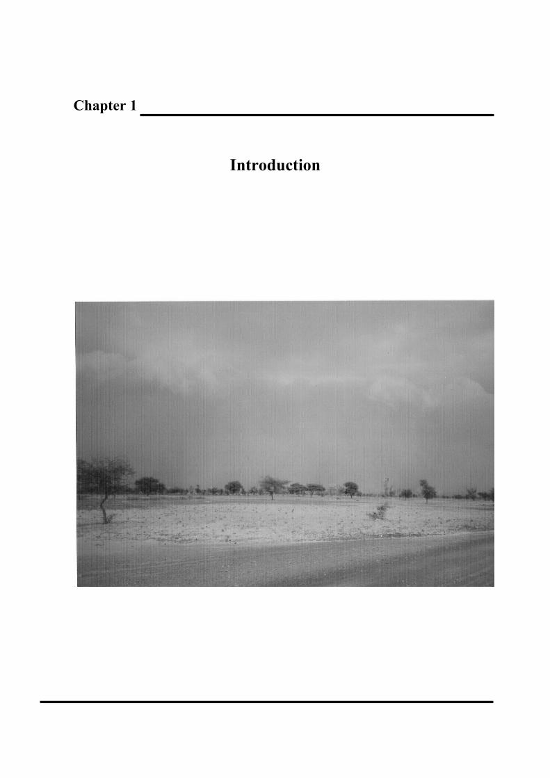
1 Introduction 1.1 Setting The Sahelian zone of Africa is one of the poorest regions of the world (Hillel, 1991). With the exception of Nigeria all Sahelian countries are classified as so-called least developed countries, because of a low per capita income, a low level of human resource development and a high degree of economic vulnerability (UN, 2004). For many people in the Sahel, living conditions are characterized by a lack of basic needs and a minimum nutritional diet is not ensured (Leisinger and Schmitt, 1995). About 90 % of the population in the Sahel depends on rainfed agriculture for their livelihood. In the last two decades, the pressure on food resources increased even more because of an increase in population (Breman et al., 2001).
Food production in the Sahel is complicated because the region is subject to a high interannual and interdecadal variability in rainfall (Hulme, 2001). But, it wasn’t until the 1980’s, that Sahelian drought drew worldwide attention. At this time the effects of a long lasting dry episode that started in 1968 became clear. The adaptive strategies that farmers had developed over the years were not sufficient to cope the drought (Mortimore and Adams, 2001). Millions of people faced famine as well as social and economic disruption (Valentin, 1995). There were hundred thousands drought related deaths among people, and millions among livestock (Batterbury and Warren, 2001). The situation highlighted the vulnerability of the region and the necessity of understanding the processes that cause and result from drought. It is within this framework that research on population growth, intensified use of natural resources and soil degradation by wind and water in the Sahel got attention.
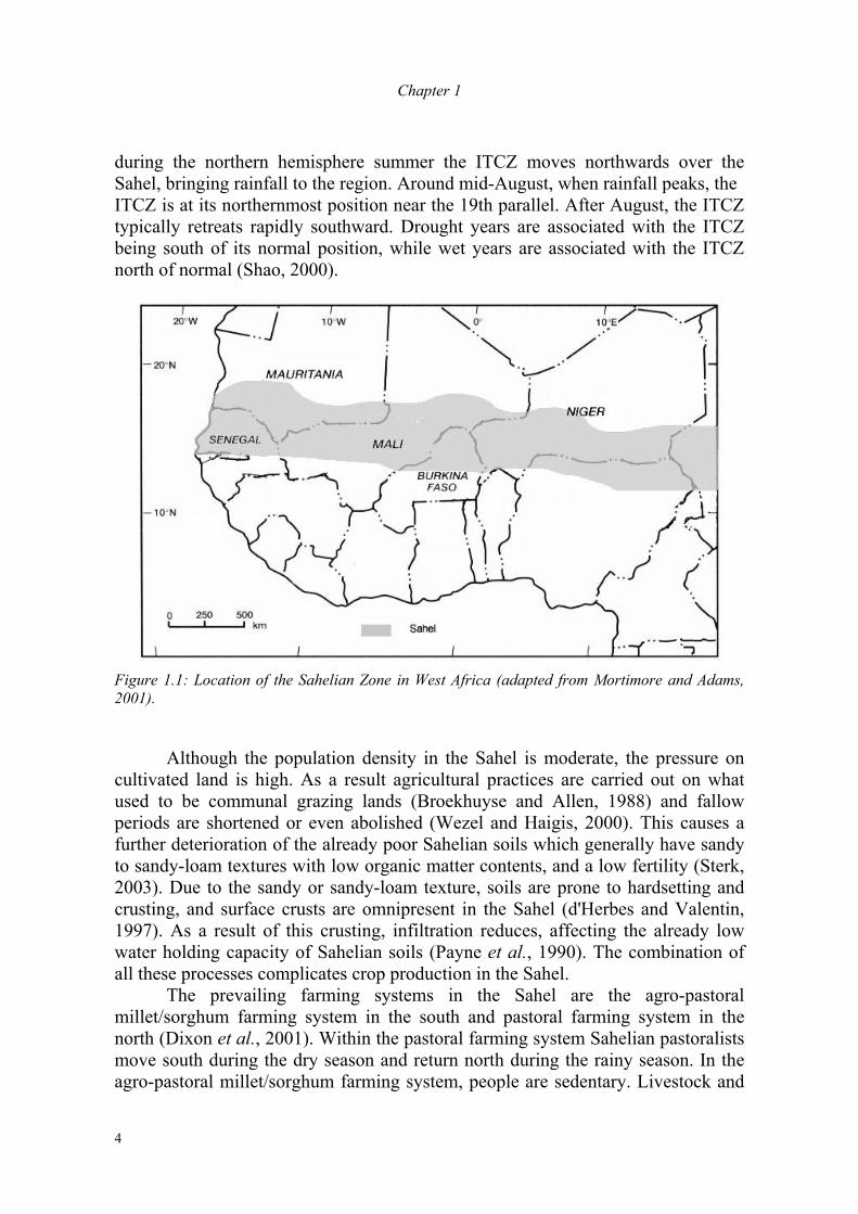
Geographically, the Sahel is a zone of about 5000 km long and 300 km wide, bordering the Sahara desert to the south. The borders of the Sahel correspond roughly with a mean annual rainfall of 200 mm in the north and 600 mm in the south (Le Houérou and Popov, 1981). These borders agree approximately to 13º and 17º Northern Latitude. In West Africa, the Sahel covers significant parts of Senegal, Mauritania, Mali, Burkina Faso, Niger, Nigeria and Chad (Figure 1.1).
The climate of the Sahel is semi-arid, with a long dry season from October to May and a short rainy season from June to September. The average temperature is high all year round. The period of rainfall in the Sahel is associated with the movement of the Inter Tropical Convergence Zone (ITCZ), located where trade winds of the northern and southern hemispheres come together. As such, the ITCZ, also known as the Intertropical Front (ITF) or the Intertropical Discontinuity (ITD), represents the boundary between dry, hot air to the north and warm, humid air to the south. During most of the year the ITCZ is located south of the Sahel. But
Chapter 1
4
during the northern hemisphere summer the ITCZ moves northwards over the Sahel, bringing rainfall to the region. Around mid-August, when rainfall peaks, the ITCZ is at its northernmost position near the 19th parallel. After August, the ITCZ typically retreats rapidly southward. Drought years are associated with the ITCZ being south of its normal position, while wet years are associated with the ITCZ north of normal (Shao, 2000).
Figure 1.1: Location of the Sahelian Zone in West Africa (adapted from Mortimore and Adams, 2001).
Although the population density in the Sahel is moderate, the pressure on
cultivated land is high. As a result agricultural practices are carried out on what used to be communal grazing lands (Broekhuyse and Allen, 1988) and fallow periods are shortened or even abolished (Wezel and Haigis, 2000). This causes a further deterioration of the already poor Sahelian soils which generally have sandy to sandy-loam textures with low organic matter contents, and a low fertility (Sterk, 2003). Due to the sandy or sandy-loam texture, soils are prone to hardsetting and crusting, and surface crusts are omnipresent in the Sahel (d'Herbes and Valentin, 1997). As a result of this crusting, infiltration reduces, affecting the already low water holding capacity of Sahelian soils (Payne et al., 1990). The combination of all these processes complicates crop production in the Sahel.
The prevailing farming systems in the Sahel are the agro-pastoral millet/sorghum farming system in the south and pastoral farming system in the north (Dixon et al., 2001). Within the pastoral farming system Sahelian pastoralists move south during the dry season and return north during the rainy season. In the agro-pastoral millet/sorghum farming system, people are sedentary. Livestock and
Introduction
5
crops are of equal importance in these systems. Pearl millet (Pennisetum glaucum) and to a lesser extent, sorghum (Sorghum bicolor) are the main crops, which can be intercropped with cowpea (Vigna unguiculata). Generally, sorghum is cultivated more southwards than pearl millet. Commonly natural woody vegetation occurs scattered in cultivated or recently fallowed fields. This allows cropping and livestock farming practices to be integrated and combined with management of trees (Petit, 2003). This kind of system is also referred to as ‘parkland system’ (Boffa, 1999). The presence of trees in the (recently) cultivated areas is highly appreciated by farmers because of the products of the trees. For example gum, wood, edible fruits and leaves are used as food, fodder or merchandise (Petit, 2003). There is a wide range in types of parkland systems. Mostly, they are characterized by the dominance of one or a few species; however, some parkland systems include a wide variety of species, without apparent dominance.
1.2 Wind Erosion Processes and Problems Wind erosion is a widespread phenomenon throughout the Sahel (Sterk, 2003). It occurs whenever the soil is loose, dry bare or nearly bare and the wind velocity exceeds the threshold velocity for initiation of soil particle movement (Fryrear and Skidmore, 1985). Soils in the Sahel are susceptible to wind erosion, as they generally have a sandy texture, and are mostly bare except for a few months in the growing season. As a consequence the amounts of wind erosion that can occur at a farmers’ field can be considerable (Sterk, 2003).
There are two distinct periods for wind erosion in the Sahel. The first is during the dry season, when the ITCZ is located to the south of the Sahel. In this period the trade winds from the Sahara, also known as the ‘Harmattan’ carry dust from the Sahara over large distances (Alfaro et al., 2004). Part of this nutrient enriched dust is deposited in the Sahel, increasing the nutrient content of the Sahelian zones (Rampsberger et al., 1998). The second and most important wind erosion period occurs in the early rainy season, when the ITCZ moves northward. During this period large thunderstorms may develop that bring the first rains of the season. The rains are often preceded by strong heavy winds causing the typical dust storms of the Sahel (Shao, 2000). These dust storms are usually of short duration, 10 – 30 minutes, but may cause serious wind erosion (Michels, 1994; Sterk, 1997).
When sediment material is entrained it can be transported by different transport modes. Generally, sand transport starts in the saltation transport mode; the bouncing motion of particles of sizes of ± 70 – 1000 µm (Shao, 2000). A sand particle can jump several millimeters to several metres along the surface. The impact of grains at the end of a bouncing trajectory might cause other particles to be dislodged either in saltation, suspension or creep mode. Particles that are transported in the suspension mode are fine dust particles (± < 70 µm). Once in suspension, the particles are easily dispersed away from the surface and travel large
Chapter 1
6
distances up to thousands of kilometers (Alfaro et al., 2004). Particles larger than 1000 µm generally are too heavy to be lifted from the surface by wind. But they can be pushed by wind or saltating particles to roll and slide along the soil surface over short distances in the creep transport mode (Shao, 2000).
Wind erosion has several negative effects. It can result in severe soil degradation by the loss of relatively fertile top soil material (Sterk et al., 1996) but it can also result in sedimentation at undesired places e.g. irrigation channels (Mohammed et al., 1995). In addition it might cause health problems due to the occurrence of large amounts of dust in the air (Alfaro et al., 2004), and it can cause crop damage due to abrasion or burial by sand during storms (Sterk and Haigis, 1998). 1.3 Wind Erosion Control in the Sahel To diminish the damage of wind erosion and to increase crop production, control measures can be used to reduce the wind velocity at the soil surface, or to increase the resistance of the soil to the forces of the wind. However, at present, adequate wind erosion control is not applied in the Sahel. Measures which have proven to be very effective in other parts of the world, such as leaving post-harvest crop residue as a flat mulch on the soil (Siddoway et al., 1965), cover crops (Tibke, 1988) or wind barriers (Borelli et al., 1989), are not widely adopted in the Sahel region. There are several reasons for not adopting these measures. For example, there is not enough mulch material available to protect the soil sufficiently as the biomass production is low (Manu et al., 1991) and crop residues are also used for fuel, fodder and construction material (Michels et al., 1995). Cover crops and wind barriers are not applied in the Sahel because of the competition for water and nutrients with crops (Sterk and Haigis, 1998). Also the variable wind directions during storms pose a problem in the planning of wind barriers. In addition to these drawbacks, farmers also might not adopt wind erosion control measures because they rank wind erosion as a low constraint to crop production relative to other problems (Bielders et al., 2001), or because they are not aware of certain measures (Visser et al., 2003). In addition, lack of labour and resources to implement measures are of importance as well (Bielders et al., 2001; Visser et al., 2003). A successful implementation and adoption of a control measure only occurs when it actually fits into the local farming system (Baidu-Forson and Napier, 1998) and when the strategy is developed by both farmers and scientists by means of a participatory development project (Van Dissel and De Graaff, 1998).
In Niger, farmers mentioned the potential of the parkland system and especially the regeneration of natural woody vegetation to reduce wind erosion (Sterk and Haigis, 1998; Taylor-Powell, 1991). Studies done by Bielders et al. (2001) and Rinaudo (1996) also pointed out that use of the parkland system could be a promising wind erosion control strategy in the Sahel. There are several reasons
Introduction
7
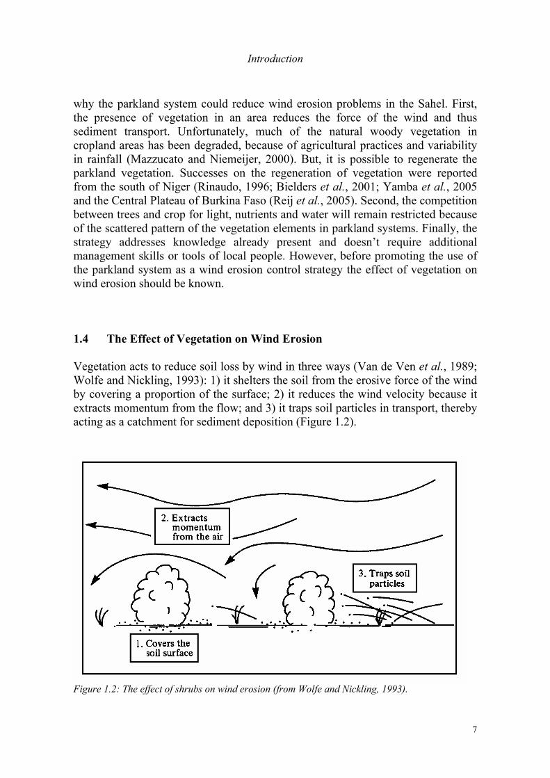
why the parkland system could reduce wind erosion problems in the Sahel. First, the presence of vegetation in an area reduces the force of the wind and thus sediment transport. Unfortunately, much of the natural woody vegetation in cropland areas has been degraded, because of agricultural practices and variability in rainfall (Mazzucato and Niemeijer, 2000). But, it is possible to regenerate the parkland vegetation. Successes on the regeneration of vegetation were reported from the south of Niger (Rinaudo, 1996; Bielders et al., 2001; Yamba et al., 2005 and the Central Plateau of Burkina Faso (Reij et al., 2005). Second, the competition between trees and crop for light, nutrients and water will remain restricted because of the scattered pattern of the vegetation elements in parkland systems. Finally, the strategy addresses knowledge already present and doesn’t require additional management skills or tools of local people. However, before promoting the use of the parkland system as a wind erosion control strategy the effect of vegetation on wind erosion should be known. 1.4 The Effect of Vegetation on Wind Erosion Vegetation acts to reduce soil loss by wind in three ways (Van de Ven et al., 1989; Wolfe and Nickling, 1993): 1) it shelters the soil from the erosive force of the wind by covering a proportion of the surface; 2) it reduces the wind velocity because it extracts momentum from the flow; and 3) it traps soil particles in transport, thereby acting as a catchment for sediment deposition (Figure 1.2).
Figure 1.2: The effect of shrubs on wind erosion (from Wolfe and Nickling, 1993).
Chapter 1
8
In this study it is hypothesised that the type of vegetation element determines the effectiveness of sediment transport reduction at different scales. A distinction is made in vegetation elements whose branches reach down to the soil surface, and vegetation elements with a canopy above a trunk. The first type of vegetation elements is referred to as shrubs and the second as trees. Behind shrubs, a wake region exists in which wind speed, and thus sediment transport, is expected to reduce. Furthermore, shrubs affect the process of wind erosion by trapping soil particles due to their low branches. For trees, an increased sediment transport is expected directly around the trunk of a tree. Below the canopy, around the trunk, streamlines are contracted, resulting in an increased wind speed and sediment transport. Thus whereas shrubs are expected to reduce sediment transport immediately around the element, trees are expected to increase sediment transport. However, in addition to these local effects, both shrubs and trees affect the process of wind erosion also on a larger scale by extracting momentum from the air, causing a reduction in wind speed in an area. As trees are generally larger in height and width than shrubs, it is expected that trees are more effective in reducing the wind speed on this larger scale than shrubs. The spacing between vegetation elements in an area determines the soil surface protected from soil erosion, but until present, the number of vegetation elements necessary to acquire an optimal protection from wind erosion is unknown (Wolfe and Nickling, 1993). 1.5 Aim The aim of this study was to determine the effects of scattered woody vegetation elements (shrubs and trees) on wind erosion processes in the Sahelian zone of Burkina Faso. The fourfold objectives of study were:
1) to determine the most common species of shrubs and trees in the Sahelian zone of Burkina Faso and evaluate the local knowledge of their impact on wind speed, sediment transport and crop production.
2) to study the relation between wind characteristics and saltation transport. 3) to quantify wind speed and sediment transport around isolated vegetation
elements in a farmers’ field in the Sahelian zone of Burkina Faso. 4) to model wind-blown sediment transport in relation to dispersed trees and
shrubs.
Introduction
9
1.6 Study Outline Fieldwork for this thesis was done during three measurement campaigns in northern Burkina Faso. The first campaign was from June until August in 2001 when a survey among farmers in three villages in northern Burkina Faso was carried out. In addition a survey was done on vegetation species present in the area. With these activities, knowledge was obtained on the distribution of the different vegetation species, their role in farming systems in general and within farmers’ fields in particular. Farmers’ perceptions of the effects of woody natural vegetation on wind erosion were also evaluated. The results of these activities are described in Chapter 2. The second and third campaigns were carried out from May to September in 2002 and 2003. During these campaigns experimental work was done in two farmers’ fields that differed with respect to the density and characteristics of the vegetation present. In one of the fields, detailed field measurements of wind speed and sediment transport were performed to study the processes that cause sediment transport and to study the effects of single vegetation elements on the alteration of wind speed and sediment transport. Chapter 3 reports on the relation between wind characteristics and the entrainment and transport of sediment. In particular the relation between wind speed, shear stress and saltation transport are described. Chapter 4 describes how single vegetation elements affect wind speed and sediment transport. In this chapter, first an overview is given of the effects of sparse vegetation and single vegetation elements on wind erosion, as known from literature. Subsequently results are presented of experimental work on the pattern of wind speed and sediment transport around isolated vegetation elements.
The knowledge that was obtained from these detailed measurements was used to develop a model that simulates the effects of single vegetation elements on wind speed and sediment transport. The developed model is spatial explicit and dynamic, i.e. it simulates sediment transport in short intervals during a storm event. Chapter 5 discusses the development and performance of this model compared to field measurements around a single vegetation element. In Chapter 6, this model is adapted to apply it to the scale of a field. The developed model was tested with data obtained during storm events in two farmers’ fields and was used to determine the effect of vegetation characteristics, the number of elements, as well as their distribution on sediment transport. Based on these modelling results, and on the results of Chapters 2 – 5, conclusions were drawn on the optimal use of scattered woody vegetation as a strategy to control wind erosion in cropland. Finally Chapter 7 summarises the main conclusions of this thesis.
Chapter 1
10
References Alfaro S.C., Rajot J.L., Nickling W. 2004: Estimation of PM20 emissions by wind erosion: main
sources of uncertainties. Geomorphology 59: 63-74. Baidu-Forson J., Napier T.L. 1998: Wind erosion control within Niger. Journal of Soil and Water
Conservation 53: 120-125. Batterbury S., Warren A. 2001: Viewpoint: The African Sahel 25 years after the great drought:
assessing progress and moving towards new agendas and approaches. Global Environmental Change 11: 1-8.
Bielders C.L., Alvey S., Cronyn N. 2001: Wind erosion: The perspective of grass-roots communities in the Sahel. Land Degradation & Development 12: 57-70.
Boffa J.M. 1999: Agroforestry parklands in sub-Saharan Africa. FAO Conservation Guide 34 FAO. Rome. 231 pp.
Borelli J., Gregory J.M., Abtew W. 1989: Wind barriers: A re-evaluation of height, spacing and porosity. Transactions of the ASAE 32: 2023-2027.
Breman H., Groot J.J.R., van Keulen H. 2001: Resource limitations in Sahelian agriculture. Global Environmental Change 11: 59-68.
Broekhuyse J.T., Allen A.M. 1988: Farming systems research. Human Organization 47: 330-342. d'Herbes J.M., Valentin C. 1997: Land surface conditions of the Niamey region: ecological and
hydrological implications. Journal of Hydrology 188-189: 18 - 42. Dixon J., Gulliver A., Gibbon D. 2001: Farming systems and poverty: Improving farmers'
livelihoods in a changing world. FAO and Worldbank. Rome and Washington DC. 412 pp.
Fryrear D.W., Skidmore E.L. 1985: Methods for controlling wind erosion. pp 443-457. In: R. F. Follet and B. A. Stewart (Eds.). Soil Erosion and Crop Productivity. American Society of Agronomy, Madison, WI, 533 pp.
Hillel D.J. 1991: Out of the earth: Civilization and the life of the soil. London: Aurum. 321 pp. Hulme M. 2001: Climatic perspectives on Sahelian desiccation: 1973-1998. Global Environmental
Change 11: 19-29. Le Houérou H.N., Popov G.F. 1981: An eco-climatic classification of intertropical Africa. FAO
Plant Production and Protection Paper 31. Leisinger K.M., Schmitt K. 1995: Survival in the Sahel. International Service for National
Agricultural Research. The Hague, The Netherlands. 211 pp. Manu A., Bationo A., Geiger S.C. 1991: Fertility status of selected millet producing soils of West
Africa. Soil Science 152: 315-320. Mazzucato V., Niemeijer D. 2000: Rethinking soil and water consrvation in a changing society, a
case study in eastern Burkina Faso. Department of Environmental Sciences, Erosion and Soil and Water Conservation Group, Wageningen University. Wageningen, The Netherlands, 380 pp.
Michels K. 1994: Wind Erosion in the Southern Sahelian Zone. Extent, Control and Effects on Millet Production. Institut für Pflanzenproduktion in den Tropen und Subtropen, Universität Hohenheim. Hohenheim, Germany, 99 pp.
Michels K., Sivakumar M.V.K., Allison B.E. 1995: Wind erosion control using crop residue I. Effects on soil flux and soil properties. Field Crops Research 40: 101-110.
Mohammed A.E., Stigter C.J., Adam H.S. 1995: Moving sand and its consequences on and near a severely desertified environment and a protective shelterbelt. Arid Soil Research and Rehabilitation 9: 423-435.
Mortimore M.J., Adams W.M. 2001: Farmer adaptation, change and 'crisis' in the Sahel. Global Environmental Change 11: 49-57.
Payne W.A., Wendt C.W., Lascano R.J. 1990: Root zone water balances of three low-input millet fields in Niger, West Africa. Journal of Arid Environments 28: 13-30.
Introduction
11
Petit S. 2003: Parklands with fodder trees: a Fulbe response to environment and social changes. Applied Geography 23: 205-225.
Rampsberger B., Hermann L., Stahr K. 1998: Dust characteristics and source-sink relations in eastern West Africa (SW-Niger and Benin) and South America (Argentinean pampas). Zeitschrift fur Pflanzenernahrung und Bodenkunde 161: 357-363.
Reij C., Tappan G., Belemvire A. 2005: Changing land management practices and vegetation on the Central Plateau of Burkina Faso (1968-2002). Journal of Arid Environments 63: 642-659.
Rinaudo T. 1996: Tailoring wind erosion control methods to farmers' specific needs. pp 161-171. In: B. Buerkert, et al. (Eds.). Proceedings of the International Symposium on 'Wind Erosion in West Africa: The Problem and its Control', Hohenheim, Germany, 5-7 December 1994. Margraf Verlag, Weikersheim, Germany.
Shao Y. 2000: Physics and modelling of wind erosion. Atmospheric and Oceanographic Sciences Library, Vol. 23, Kluwer Academic Publishers. Dordrecht, The Netherlands. 393 pp.
Siddoway F.H., Chepil W.S., Armbrust D.V. 1965: Effect of kind, amount and placement of residue on wind erosion control. Transactions of the ASAE 8: 327-331.
Sterk G. 1997: Wind erosion in the Sahelian zone of Niger: Processes, models and control techniques. Department of Irrigation and Soil and Water Conservation, Wageningen Agricultural University. Wageningen, The Netherlands, 152 pp.
Sterk G. 2003: Causes, consequences and control of wind erosion in Sahelian Africa: A review. Land Degradation & Development 14: 95-108.
Sterk G., Haigis J. 1998: Farmers' knowledge of wind erosion processes and control methods in Niger. Land Degradation & Development 9: 107-114.
Sterk G., Hermann L., Bationo A. 1996: Wind-blown nutrient transport and soil poductivity changes in southwest Niger. Land Degradation & Development 7: 325-335.
Taylor-Powell E. 1991: Integrated management of agricultural watersheds: Land tenure and indigenous knowledge of soil and crop management. Tropical Soils Bulletin 91-04, Texas A&M University: College Station. TX, USA.
Tibke G. 1988: Basic principles of wind erosion control. Agriculture, Ecosystems & Environment 22/23: 103-122.
UN. 2004: Report of the Committee on Development Policy on its sixth session. E/2004/33. United Nations. New York, USA. 33 pp.
Valentin C. 1995: Sealing, crusting and hardsetting soils in Sahelian agriculture. pp 53-76. In: H. B. So, et al. (Eds.). Sealing, Crusting and Hardsetting Soils: Productivity and Conservation. Australian Society of Soil Science, Brisbane, Australia.
Van de Ven T.A.M., Fryrear D.W., Spaan W.P. 1989: Vegetation characteristics and soil loss by wind. Journal of Soil and Water Conservation 44: 347-349.
Van Dissel S.C., De Graaff J. 1998: Differences between farmers and scientists in the perception of soil erosion: A south African case study. Indigenous Knowledge and Development Monitor 6: 8-9.
Visser S.M., Leenders J.K., Leeuwis M. 2003: Farmers' perceptions of erosion by wind and water in northern Burkina Faso. Land Degradation & Development 14: 123-132.
Wezel A., Haigis J. 2000: Famers' perception of vegetation changes in semi-arid Niger. Land Degradation & Development 11: 523-534.
Wolfe S.A., Nickling W.G. 1993: The protective role of sparse vegetation in wind erosion. Progress in Physical Geography 17: 50-68.
Yamba B., Mahamane L., Abdou H., Reij C. 2005: Rapport Etude de Pilote Niger (25 janvier au 10 février 2005). International Resources Group (IRG), Comité Inter-Etats de Lutte contre la Sécheresse au Sahel (CILSS). 30 pp.

Chapter 2
Farmers’ Perceptions of the Role of Scattered Vegetation in Wind Erosion Control on
Arable Land in Burkina Faso
Leenders J.K., Visser S. M. and Stroosnijder L. In: Land Degradation & Development 16: 327 – 337 (2005)

Farmers’ Perceptions of the Role of Scattered Vegetation
15
2 Farmers’Perceptions of the Role of Scattered
Vegetation in Wind Erosion Control on Arable Land in Burkina Faso.
Abstract This paper describes the results of a survey on farmers’ perceptions of the effect of woody natural vegetation on wind erosion. Sixty farmers were interviewed in three villages in northern Burkina Faso. The farmers mentioned that the presence of woody vegetation between the crops could benefit yield, but feared competition between the natural vegetation and the crop. Vegetation in a field was considered to increase deposition and decrease erosion on that field. The most important vegetative characteristics that affect wind erosion were, according to the farmers, vegetation’s shape, porosity, flexibility and arrangement of the vegetation in the field. At present, most farmers do not apply this knowledge to the management of the natural woody vegetation on their fields. 2.1 Introduction Sahelian Africa is one of the regions in the world where there is an imbalance between food demand and food supply. The population, and thus the food demand, has increased by more than 3 per cent per year in the last two decades, whereas the rate of food supply was around 2 per cent (Breman et al., 2001). To enhance food production, farmers did not intensify their farming systems, but they expanded the cropped area (Sterk, 2003) and diminished or abolished the fallow period (Wezel and Haigis, 2002). As a result the marginal lands, which used to be communal grazing land, are now cropped (Broekhuyse and Allen, 1988) and land degradation and desertification occur at a large scale (Hillel, 1991). In fact, the Sahelian zone of Africa is the region of the world that is most subjected to desertification (Valentin, 1995). In Burkina Faso 50 per cent of the total land area is classified as highly to very highly vulnerable for desertification, only 12 per cent of the total land area is estimated as not being vulnerable for desertification (Reich et al., 2001). Wind erosion is a widespread phenomenon throughout the Sahel (Sterk, 2003). It can occur whenever the soil is loose, dry bare or nearly bare and the wind velocity exceeds the threshold velocity for initiation of soil-particle movement (Fryrear and Skidmore, 1985). In the Sahel agricultural lands are liable to wind erosion (Sterk, 2003). The sandy-textured soils are, except for a few months in the growing season, bare and loose and without adequate measures for wind erosion control. The combination of these soil conditions and the severe winds that occur at the onset of the rainy season makes the area susceptible to wind erosion. The amounts of wind erosion that can occur at a farmers’ field can be considerable (Sterk, 2003).
Chapter 2
16
Wind erosion has a negative effect on crop production. Its effects may be threefold: 1) soil degradation, 2) crop damage and 3) sedimentation at undesired places (Sterk, 2003). To diminish the damage of wind erosion and to increase crop production, control measures can be used to reduce the wind velocity at the soil surface, or to help the soil resist the forces of the wind. However, at present, no adequate wind erosion control measure exists for the Sahel. Measures that have proven to be very effective in other parts of the world, such as leaving post-harvest crop residue as a flat mulch on the soil (Siddoway et al., 1965), cover crops (Tibke, 1988) or wind barriers (Borelli et al., 1989), are not widely applied or adopted in the Sahel region. They do not fit into the local farming system. Mulch material, for example, is in too short supply to protect the soil sufficiently as the crop production is low (Manu et al., 1991) and crop residues are also used for fuel, fodder and construction material (Michels et al., 1995). Cover crops and windbreaks are not applied in the Sahel because of the competition for water and nutrients (Sterk and Haigis, 1998). A successful implementation and adoption of a control measure only occurs when it actually fits into the local farming system (Baidu-Forson and Napier, 1998). This can only be achieved by developing a control strategy for both farmers and scientists by means of a participatory project (Van Dissel and De Graaff, 1998). In Niger, farmers mentioned the potential of the natural woody vegetation in cropland, the so-called parkland system, to reduce wind erosion (Sterk and Haigis, 1998; Taylor-Powell, 1991). A parkland system is a landscape in which mature trees occur scattered in cultivated or recently fallowed fields. The system allows the integration of cropping and livestock farming practices in combination with the management of trees (Petit, 2003). Parkland systems are very common in the Sahel (Boffa, 1999) and highly appreciated by farmers because the products of trees e.g. gum, wood, edible fruits and leaves are used as food, fodder or merchandise (Petit, 2003). There is a wide range in types of parkland systems. Mostly, they are characterized by the dominance of one or a few species. However, some parkland systems include a wide variety of species, without apparent dominance. To capture regional and local variation in parkland structure and composition, factors as degree of human intervention, main functional uses, physical structure and reflection of the different natural resource management systems of the diverse ethnic groups should be taken into account (Boffa, 1999). Studies undertaken by Bielders et al. (2001) and Rinaudo (1994) also point out that use of the parkland system could be a promising wind erosion control strategy in the Sahel. It seems promising because of several reasons. First, the presence of standing natural vegetation amongst the crop covers and protects the soil surface, diminishes the net force of the wind on the soil surface and traps soil particles (Van de Ven et al., 1989). Second, the competition between trees and the crop for light, nutrients and water remains restricted because of the scattered pattern of the trees. Finally, the measure addresses knowledge already present and doesn’t require additional management skills or tools from the local people.
Farmers’ Perceptions of the Role of Scattered Vegetation
17
In this study the use of the parkland system as a wind erosion control strategy is studied among sixty farmers in the north of Burkina Faso. The research objectives were: 1) to obtain insight into the farming system and the problem of wind erosion to the farmers in the research area; 2) to evaluate the occurrence and use of the natural vegetation present in the area; and 3) to evaluate farmers’ knowledge on the effect of vegetation on crop production and wind erosion as well as the present use of this knowledge. 2.2 Research Area The study area is located in the north of Burkina Faso, which is part of the southern Sahelian zone. The Sahelian zone of Africa (the Sahel) is situated between the latitudes 13º N and 16º N, the isohyet of 200 mm borders the zone in the north and the one of 600 mm in the south. The Sahelian Zone can be seen as the transition zone between the arid Sahara in the north and the more humid Sudanian Zone in the south (Le Houérou and Popov, 1981). From north to south average annual rainfall progressively increases and with this change in rainfall the vegetation and land-use characteristics also change. From east to west, there is not much variation in average annual rainfall or in vegetation and land-use characteristics. (Breman and de Ridder, 1991).
Wind erosion in the Sahel may occur during two distinct periods. The first period is during the dry season (October to April), when the area is subjected to dry, north-easterly trade winds, originating from a dry continental airmass above the Sahara Desert. These trade winds are known as the Harmattan and may result in low to moderate wind erosion (Michels et al., 1995). The second and most important period for wind erosion is the early rainy season (May to July). At this period, the tropical maritime anticyclone to the south of West Africa expands (Hayward and Oguntoyinbo, 1987), pushing the Harmattan winds northward and bringing warm, moist air and rain to the area. The strong winds that precede a rain event, last for only 10 to 30 minutes, but may result in intense particle movement (Michels et al., 1995). Although there exists a wide variety in woody species among parkland systems in the Sahel, Pullan (1974) mentioned some dominant species for the Sahel. They are thorny trees and shrubs, which are well adapted to the harsh climate: Acacia raddiana, Balanites aegyptiaca, Hyphaene thebaica, Acacia senegal, Tamarindus indica, Piliostigma reticulatum and Borassus aethiopum. The most common herbaceous species are Panicum laetum, Cassia tora, Aristida adscensionis and Schoenefeldia gracilis (Fontès and Guinko, 1995).
The research was conducted in three typical Sahelian villages in Seno Province, in the north of Burkina Faso. The villages, Dangadé, Katchari and Sambonaye, are within 25 km of Dori, the provincial capital (14º00’N to 0º10’W) (Figure 2.1). The average annual precipitation in the area is 420 mm. However, the
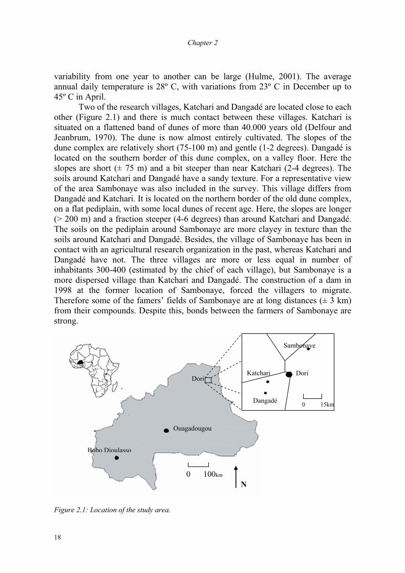
Chapter 2
18
variability from one year to another can be large (Hulme, 2001). The average annual daily temperature is 28º C, with variations from 23º C in December up to 45º C in April.
Two of the research villages, Katchari and Dangadé are located close to each other (Figure 2.1) and there is much contact between these villages. Katchari is situated on a flattened band of dunes of more than 40.000 years old (Delfour and Jeanbrum, 1970). The dune is now almost entirely cultivated. The slopes of the dune complex are relatively short (75-100 m) and gentle (1-2 degrees). Dangadé is located on the southern border of this dune complex, on a valley floor. Here the slopes are short (± 75 m) and a bit steeper than near Katchari (2-4 degrees). The soils around Katchari and Dangadé have a sandy texture. For a representative view of the area Sambonaye was also included in the survey. This village differs from Dangadé and Katchari. It is located on the northern border of the old dune complex, on a flat pediplain, with some local dunes of recent age. Here, the slopes are longer (> 200 m) and a fraction steeper (4-6 degrees) than around Katchari and Dangadé. The soils on the pediplain around Sambonaye are more clayey in texture than the soils around Katchari and Dangadé. Besides, the village of Sambonaye has been in contact with an agricultural research organization in the past, whereas Katchari and Dangadé have not. The three villages are more or less equal in number of inhabitants 300-400 (estimated by the chief of each village), but Sambonaye is a more dispersed village than Katchari and Dangadé. The construction of a dam in 1998 at the former location of Sambonaye, forced the villagers to migrate. Therefore some of the famers’ fields of Sambonaye are at long distances (± 3 km) from their compounds. Despite this, bonds between the farmers of Sambonaye are strong.
Figure 2.1: Location of the study area.
Dori
Dangadé
Sambonaye
Katchari
0 15km
N
Dori
Ouagadougou
Bobo Dioulasso
0 100km
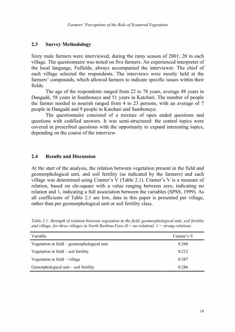
Farmers’ Perceptions of the Role of Scattered Vegetation
19
2.3 Survey Methodology Sixty male farmers were interviewed, during the rainy season of 2001; 20 in each village. The questionnaire was tested on five farmers. An experienced interpreter of the local language, Fulfulde, always accompanied the interviewer. The chief of each village selected the respondents. The interviews were mostly held at the farmers’ compounds, which allowed farmers to indicate specific issues within their fields. The age of the respondents ranged from 22 to 78 years, average 48 years in Dangadé, 58 years in Sambonaye and 51 years in Katchari. The number of people the farmer needed to nourish ranged from 4 to 23 persons, with an average of 7 people in Dangadé and 9 people in Katchari and Sambonaye. The questionnaire consisted of a mixture of open ended questions and questions with codified answers. It was semi-structured: the central topics were covered in prescribed questions with the opportunity to expand interesting topics, depending on the course of the interview. 2.4 Results and Discussion At the start of the analysis, the relation between vegetation present in the field and geomorphological unit, and soil fertility (as indicated by the farmers) and each village was determined using Cramer’s V (Table 2.1). Cramer’s V is a measure of relation, based on chi-square with a value ranging between zero, indicating no relation and 1, indicating a full association between the variables (SPSS, 1999). As all coefficients of Table 2.1 are low, data in this paper is presented per village, rather than per geomorphological unit or soil fertility class. Table 2.1: Strength of relation between vegetation in the field, geomorphological unit, soil fertility and village, for three villages in North Burkina Faso (0 = no relationl; 1 = strong relation).
Variable Cramer’s V
Vegetation in field – geomorphological unit 0.260
Vegetation in field – soil fertility 0.212
Vegetation in field – village 0.387
Gemorphological unit – soil fertility 0.286
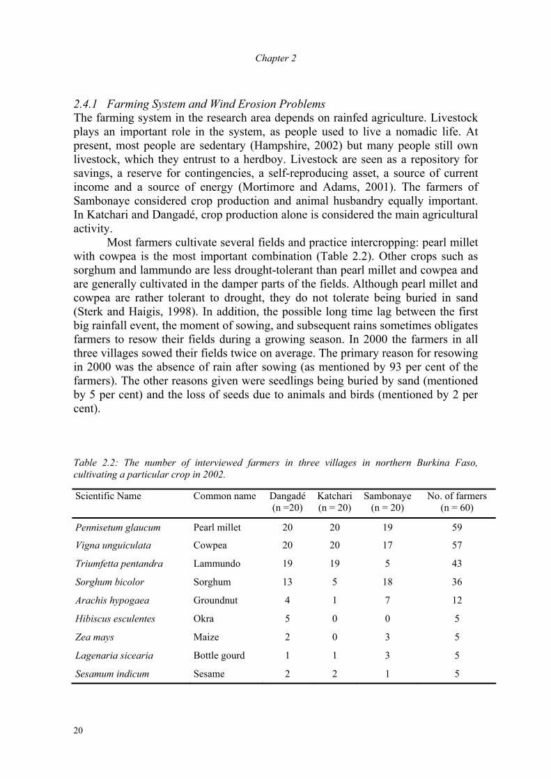
Chapter 2
20
2.4.1 Farming System and Wind Erosion Problems The farming system in the research area depends on rainfed agriculture. Livestock plays an important role in the system, as people used to live a nomadic life. At present, most people are sedentary (Hampshire, 2002) but many people still own livestock, which they entrust to a herdboy. Livestock are seen as a repository for savings, a reserve for contingencies, a self-reproducing asset, a source of current income and a source of energy (Mortimore and Adams, 2001). The farmers of Sambonaye considered crop production and animal husbandry equally important. In Katchari and Dangadé, crop production alone is considered the main agricultural activity.
Most farmers cultivate several fields and practice intercropping: pearl millet with cowpea is the most important combination (Table 2.2). Other crops such as sorghum and lammundo are less drought-tolerant than pearl millet and cowpea and are generally cultivated in the damper parts of the fields. Although pearl millet and cowpea are rather tolerant to drought, they do not tolerate being buried in sand (Sterk and Haigis, 1998). In addition, the possible long time lag between the first big rainfall event, the moment of sowing, and subsequent rains sometimes obligates farmers to resow their fields during a growing season. In 2000 the farmers in all three villages sowed their fields twice on average. The primary reason for resowing in 2000 was the absence of rain after sowing (as mentioned by 93 per cent of the farmers). The other reasons given were seedlings being buried by sand (mentioned by 5 per cent) and the loss of seeds due to animals and birds (mentioned by 2 per cent). Table 2.2: The number of interviewed farmers in three villages in northern Burkina Faso, cultivating a particular crop in 2002.
Scientific Name Common name Dangadé (n =20)
Katchari (n = 20)
Sambonaye (n = 20)
No. of farmers (n = 60)
Pennisetum glaucum Pearl millet 20 20 19 59
Vigna unguiculata Cowpea 20 20 17 57
Triumfetta pentandra Lammundo 19 19 5 43
Sorghum bicolor Sorghum 13 5 18 36
Arachis hypogaea Groundnut 4 1 7 12
Hibiscus esculentes Okra 5 0 0 5
Zea mays Maize 2 0 3 5
Lagenaria sicearia Bottle gourd 1 1 3 5
Sesamum indicum Sesame 2 2 1 5
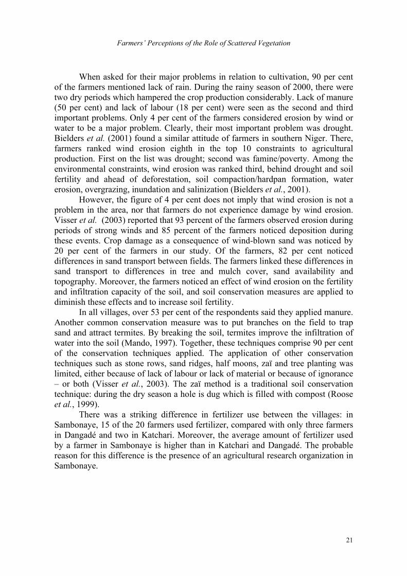
Farmers’ Perceptions of the Role of Scattered Vegetation
21
When asked for their major problems in relation to cultivation, 90 per cent of the farmers mentioned lack of rain. During the rainy season of 2000, there were two dry periods which hampered the crop production considerably. Lack of manure (50 per cent) and lack of labour (18 per cent) were seen as the second and third important problems. Only 4 per cent of the farmers considered erosion by wind or water to be a major problem. Clearly, their most important problem was drought. Bielders et al. (2001) found a similar attitude of farmers in southern Niger. There, farmers ranked wind erosion eighth in the top 10 constraints to agricultural production. First on the list was drought; second was famine/poverty. Among the environmental constraints, wind erosion was ranked third, behind drought and soil fertility and ahead of deforestation, soil compaction/hardpan formation, water erosion, overgrazing, inundation and salinization (Bielders et al., 2001).
However, the figure of 4 per cent does not imply that wind erosion is not a problem in the area, nor that farmers do not experience damage by wind erosion. Visser et al. (2003) reported that 93 percent of the farmers observed erosion during periods of strong winds and 85 percent of the farmers noticed deposition during these events. Crop damage as a consequence of wind-blown sand was noticed by 20 per cent of the farmers in our study. Of the farmers, 82 per cent noticed differences in sand transport between fields. The farmers linked these differences in sand transport to differences in tree and mulch cover, sand availability and topography. Moreover, the farmers noticed an effect of wind erosion on the fertility and infiltration capacity of the soil, and soil conservation measures are applied to diminish these effects and to increase soil fertility. In all villages, over 53 per cent of the respondents said they applied manure. Another common conservation measure was to put branches on the field to trap sand and attract termites. By breaking the soil, termites improve the infiltration of water into the soil (Mando, 1997). Together, these techniques comprise 90 per cent of the conservation techniques applied. The application of other conservation techniques such as stone rows, sand ridges, half moons, zaï and tree planting was limited, either because of lack of labour or lack of material or because of ignorance – or both (Visser et al., 2003). The zaï method is a traditional soil conservation technique: during the dry season a hole is dug which is filled with compost (Roose et al., 1999). There was a striking difference in fertilizer use between the villages: in Sambonaye, 15 of the 20 farmers used fertilizer, compared with only three farmers in Dangadé and two in Katchari. Moreover, the average amount of fertilizer used by a farmer in Sambonaye is higher than in Katchari and Dangadé. The probable reason for this difference is the presence of an agricultural research organization in Sambonaye.

Chapter 2
22
2.4.2 Occurrence and Use of Natural Vegetation Three of the most common tree and shrub species in the farmers’ fields (Acacia raddiana, Balanites aegyptiaca and Hyphaene thebaica) as mentioned by the farmers (Table 2.3), are also described by Pullan (1974) as being characteristic of the Sahelian parkland. Table 2.3: The five most common woody species present in the fields of the 60 farmers interviewed.
Dangadé (n = 192)a Katchari (n = 251)a Sambonaye (n =278)a Total (n = 721)b
Species(n= 21)c % Species(n= 20)c % Species(n= 26)c % Species(n= 32)c %
Balan aegyptiaca 15.6 Balan aegyptiaca 20.7 Acacia raddiana 13.3 Balan aegyptiaca 13.1
Faidherbia albida 13.0 Acacia raddiana 16.3 Balan aegyptiaca 12.6 Acacia raddiana 14.0
Acacia raddiana 12.5 Faidherbia alb. 12.7 Ziziphus maur. 11.9 Ziziphus maur. 10.3
Hyphaene theb. 10.4 Ziziphus maur. 10.4 Acacia seyal 09.4 Faidherbia alb. 9.6
Sclerocarya birrea
08.9 Sclerocarya birrea
09.2 Bauhinia ruf Dichostachys cin.Sclerocarya bir
06.5 06.5 06.5
Sclerocarya bir. 8.0
Remainder (16 species)
39.6 Remainder (15 species)
30.7 Remainder (18 species)
33.3 Remainder (27 species)
45.0
aNumber of statements on plant species per village. bTotal number of statements on plant species. cNumber of species mentioned. To find out whether the farmers eradicate or cut down particular species from their fields, they were also asked which species were present near their fields. As the most common species of vegetation around fields were the same as those in the fields, and the farmers mentioned more species in their fields than that around their fields (Table 2.4), it was concluded that farmers did not systematically eradicate particular species. There are no physical reasons to explain why more species were mentioned as growing in the fields than outside the fields. We suggest that the explanation is related to the farmers’ perception of the neighbourhood: vegetation in their fields lies within the area important to them; the vegetation around the fields is perceived as less important and is therefore less familiar. Species richness is higher in Sambonaye compared to Dangadé/Katchari. This is attributed to the more clayey soils of the pediplain around Sambonaye, compared to the more sandy soils of the dunes around Dangadé and Katchari. The fertilizer use by the farmers of Sambonaye, also might contribute to this. According to 96 per cent of the farmers, the overall natural vegetation has decreased during the last ten years. No specific species were mentioned as declining significantly, but most farmers (75 per cent) did give a reason for the
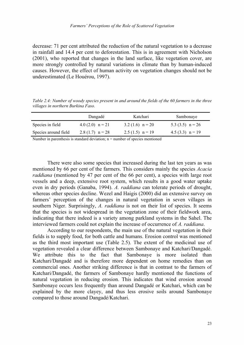
Farmers’ Perceptions of the Role of Scattered Vegetation
23
decrease: 71 per cent attributed the reduction of the natural vegetation to a decrease in rainfall and 14.4 per cent to deforestation. This is in agreement with Nicholson (2001), who reported that changes in the land surface, like vegetation cover, are more strongly controlled by natural variations in climate than by human-induced causes. However, the effect of human activity on vegetation changes should not be underestimated (Le Houérou, 1997). Table 2.4: Number of woody species present in and around the fields of the 60 farmers in the three villages in northern Burkina Faso.
Dangadé Katchari Sambonaye
Species in field 4.0 (2.0) n = 21 3.2 (1.6) n = 20 5.3 (3.5) n = 26
Species around field 2.8 (1.7) n = 28 2.5 (1.5) n = 19 4.5 (3.3) n = 19 Number in parenthesis is standard deviation; n = number of species mentioned
There were also some species that increased during the last ten years as was mentioned by 66 per cent of the farmers. This considers mainly the species Acacia raddiana (mentioned by 47 per cent of the 66 per cent), a species with large root vessels and a deep, extensive root system, which results in a good water uptake even in dry periods (Ganaba, 1994). A. raddiana can tolerate periods of drought, whereas other species decline. Wezel and Haigis (2000) did an extensive survey on farmers’ perception of the changes in natural vegetation in seven villages in southern Niger. Surprisingly, A. raddiana is not on their list of species. It seems that the species is not widespread in the vegetation zone of their fieldwork area, indicating that there indeed is a variety among parkland systems in the Sahel. The interviewed farmers could not explain the increase of occurrence of A. raddiana.
According to our respondents, the main use of the natural vegetation in their fields is to supply food, for both cattle and humans. Erosion control was mentioned as the third most important use (Table 2.5). The extent of the medicinal use of vegetation revealed a clear difference between Sambonaye and Katchari/Dangadé. We attribute this to the fact that Sambonaye is more isolated than Katchari/Dangadé and is therefore more dependent on home remedies than on commercial ones. Another striking difference is that in contrast to the farmers of Katchari/Dangadé, the farmers of Sambonaye hardly mentioned the functions of natural vegetation in reducing erosion. This indicates that wind erosion around Sambonaye occurs less frequently than around Dangadé or Katchari, which can be explained by the more clayey, and thus less erosive soils around Sambonaye compared to those around Dangadé/Katchari.
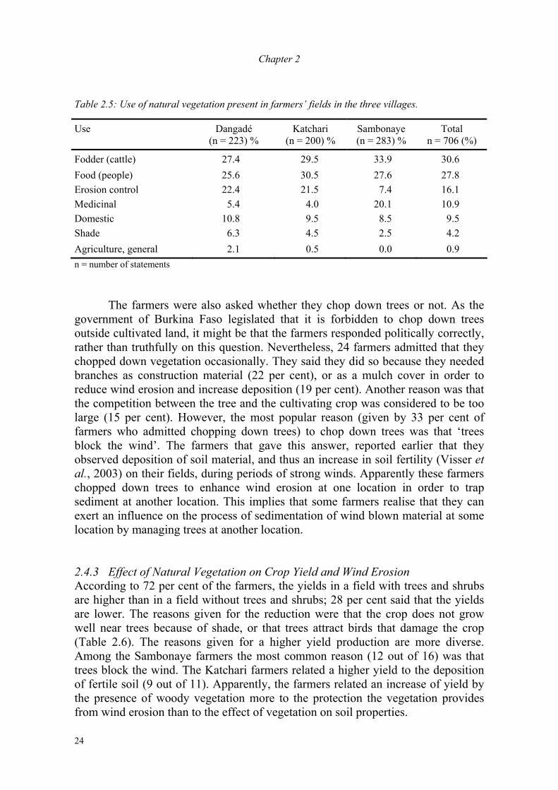
Chapter 2
24
Table 2.5: Use of natural vegetation present in farmers’ fields in the three villages.
Use Dangadé (n = 223) %
Katchari (n = 200) %
Sambonaye (n = 283) %
Total n = 706 (%)
Fodder (cattle) 27.4 29.5 33.9 30.6 Food (people) 25.6 30.5 27.6 27.8 Erosion control 22.4 21.5 7.4 16.1 Medicinal 5.4 4.0 20.1 10.9 Domestic 10.8 9.5 8.5 9.5 Shade 6.3 4.5 2.5 4.2 Agriculture, general 2.1 0.5 0.0 0.9 n = number of statements
The farmers were also asked whether they chop down trees or not. As the government of Burkina Faso legislated that it is forbidden to chop down trees outside cultivated land, it might be that the farmers responded politically correctly, rather than truthfully on this question. Nevertheless, 24 farmers admitted that they chopped down vegetation occasionally. They said they did so because they needed branches as construction material (22 per cent), or as a mulch cover in order to reduce wind erosion and increase deposition (19 per cent). Another reason was that the competition between the tree and the cultivating crop was considered to be too large (15 per cent). However, the most popular reason (given by 33 per cent of farmers who admitted chopping down trees) to chop down trees was that ‘trees block the wind’. The farmers that gave this answer, reported earlier that they observed deposition of soil material, and thus an increase in soil fertility (Visser et al., 2003) on their fields, during periods of strong winds. Apparently these farmers chopped down trees to enhance wind erosion at one location in order to trap sediment at another location. This implies that some farmers realise that they can exert an influence on the process of sedimentation of wind blown material at some location by managing trees at another location. 2.4.3 Effect of Natural Vegetation on Crop Yield and Wind Erosion According to 72 per cent of the farmers, the yields in a field with trees and shrubs are higher than in a field without trees and shrubs; 28 per cent said that the yields are lower. The reasons given for the reduction were that the crop does not grow well near trees because of shade, or that trees attract birds that damage the crop (Table 2.6). The reasons given for a higher yield production are more diverse. Among the Sambonaye farmers the most common reason (12 out of 16) was that trees block the wind. The Katchari farmers related a higher yield to the deposition of fertile soil (9 out of 11). Apparently, the farmers related an increase of yield by the presence of woody vegetation more to the protection the vegetation provides from wind erosion than to the effect of vegetation on soil properties.
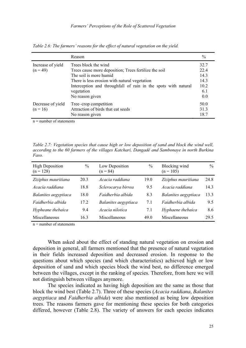
Farmers’ Perceptions of the Role of Scattered Vegetation
25
Table 2.6: The farmers’ reasons for the effect of natural vegetation on the yield.
Reason %
Increase of yield (n = 49)
Trees block the wind Trees cause more deposition; Trees fertilize the soil The soil is more humid There is less erosion with natural vegetation Interception and throughfall of rain in the spots with natural vegetation No reason given
32.7 22.4 14.3 14.3 10.2
6.1 0.0
Decrease of yield (n = 16)
Tree–crop competition Attraction of birds that eat seeds No reason given
50.0 31.3 18.7
n = number of statements Table 2.7: Vegetation species that cause high or low deposition of sand and block the wind well, according to the 60 farmers of the villages Katchari, Dangadé and Sambonaye in north Burkina Faso.
High Deposition (n = 128)
% Low Deposition (n = 84)
% Blocking wind (n = 105)
%
Ziziphus mauritiana 20.3 Acacia raddiana 19.0 Ziziphus mauritiana 24.8
Acacia raddiana 18.8 Sclerocarya birrea 9.5 Acacia raddiana 14.3
Balanites aegyptiaca 18.0 Faidherbia albida 8.3 Balanites aegyptiaca 13.3
Faidherbia albida 17.2 Balanites aegyptiaca 7.1 Faidherbia albida 9.5
Hypheane thebaica 9.4 Acacia nilotica 7.1 Hyphaene thebaica 8.6
Miscellaneous 16.3 Miscellaneous 49.0 Miscellaneous 29.5n = number of statements
When asked about the effect of standing natural vegetation on erosion and deposition in general, all farmers mentioned that the presence of natural vegetation in their fields increased deposition and decreased erosion. In response to the questions about which species (and which characteristics) achieved high or low deposition of sand and which species block the wind best, no difference emerged between the villages, except in the ranking of species. Therefore, from here we will not distinguish between villages anymore.
The species indicated as having high deposition are the same as those that block the wind best (Table 2.7). Three of these species (Acacia raddiana, Balanites aegyptiaca and Faidherbia albida) were also mentioned as being low deposition trees. The reasons farmers gave for mentioning these species for both categories differed, however (Table 2.8). The variety of answers for each species indicates
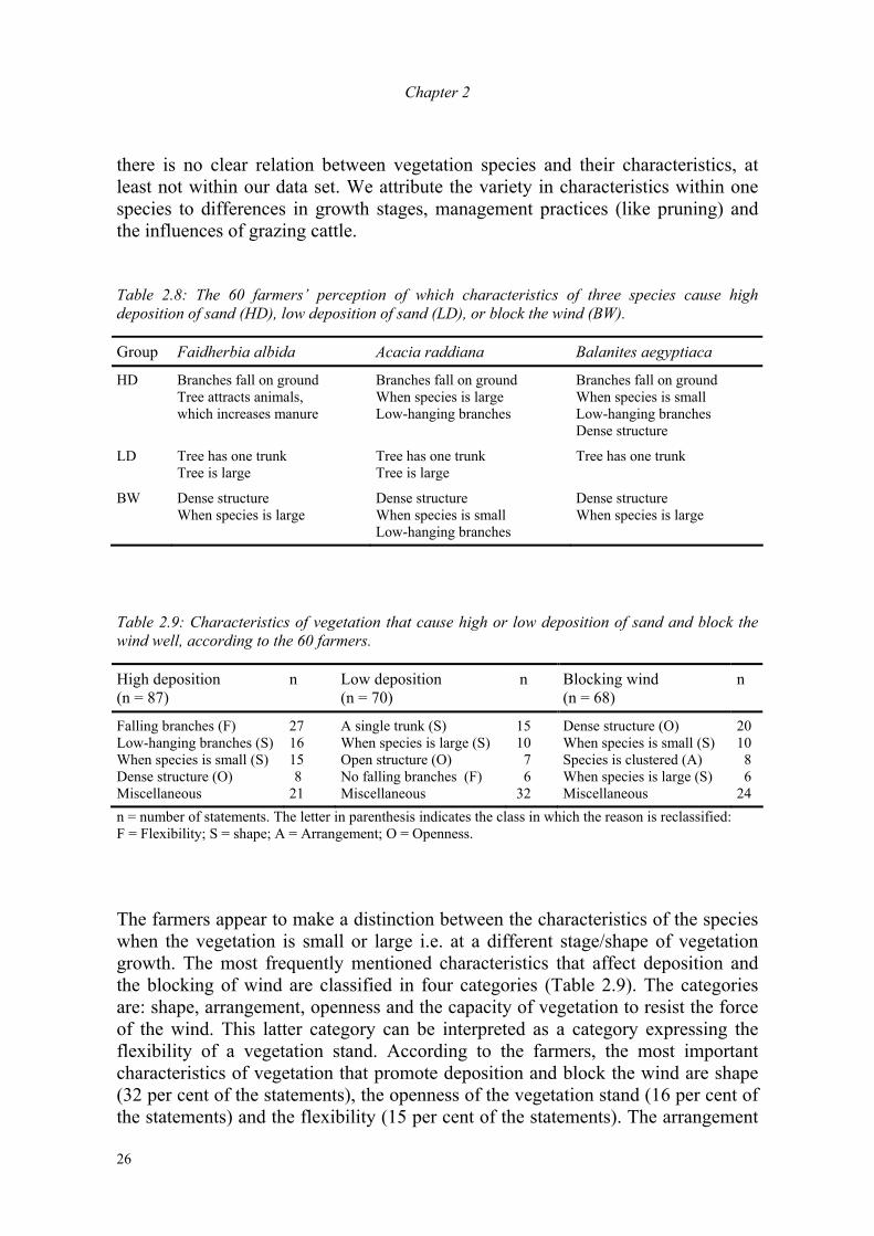
Chapter 2
26
there is no clear relation between vegetation species and their characteristics, at least not within our data set. We attribute the variety in characteristics within one species to differences in growth stages, management practices (like pruning) and the influences of grazing cattle. Table 2.8: The 60 farmers’ perception of which characteristics of three species cause high deposition of sand (HD), low deposition of sand (LD), or block the wind (BW).
Group Faidherbia albida Acacia raddiana Balanites aegyptiaca
HD
Branches fall on ground Tree attracts animals, which increases manure
Branches fall on ground When species is large Low-hanging branches
Branches fall on ground When species is small Low-hanging branches Dense structure
LD Tree has one trunk Tree is large
Tree has one trunk Tree is large
Tree has one trunk
BW Dense structure When species is large
Dense structure When species is small Low-hanging branches
Dense structure When species is large
Table 2.9: Characteristics of vegetation that cause high or low deposition of sand and block the wind well, according to the 60 farmers.
High deposition (n = 87)
n Low deposition (n = 70)
n Blocking wind (n = 68)
n
Falling branches (F) Low-hanging branches (S) When species is small (S) Dense structure (O) Miscellaneous
27 16 15 8
21
A single trunk (S) When species is large (S) Open structure (O) No falling branches (F) Miscellaneous
15 10
7 6
32
Dense structure (O) When species is small (S) Species is clustered (A) When species is large (S) Miscellaneous
20 10
8 6
24 n = number of statements. The letter in parenthesis indicates the class in which the reason is reclassified: F = Flexibility; S = shape; A = Arrangement; O = Openness. The farmers appear to make a distinction between the characteristics of the species when the vegetation is small or large i.e. at a different stage/shape of vegetation growth. The most frequently mentioned characteristics that affect deposition and the blocking of wind are classified in four categories (Table 2.9). The categories are: shape, arrangement, openness and the capacity of vegetation to resist the force of the wind. This latter category can be interpreted as a category expressing the flexibility of a vegetation stand. According to the farmers, the most important characteristics of vegetation that promote deposition and block the wind are shape (32 per cent of the statements), the openness of the vegetation stand (16 per cent of the statements) and the flexibility (15 per cent of the statements). The arrangement

Farmers’ Perceptions of the Role of Scattered Vegetation
27
of vegetation in the field was considered to be less important (5 per cent of the statements). These factors, together with height, width and cover are also mentioned in literature as being important for the effect on wind velocity (Marshall, 1970; Musick and Gillette, 1990; Wolfe and Nickling, 1993). From studies on windbreaks it is known that the windbreak porosity is the major factor determining the amount of shelter (Cleugh, 1998). Whether this holds true for isolated individual trees has not yet been investigated.
According to 46 of the 60 farmers, the best type of spatial arrangement (trees in groups, lines or single trees) to block the wind is, trees in lines, with trees in groups second best. Single trees were unanimously considered to be the least effective arrangement to block the wind. Farmers are less clear on the preferred type of arrangement at a farmers’ field (Table 2.10). Evidently there are other motivations, like tree–crop competition than wind erosion control alone for wanting a certain arrangement of vegetation in their field. Table 2.10: The 60 farmers’ preference regarding the spatial arrangement of woody natural vegetation in their fields.
Dangadé (n = 20)
Katchari (n = 20)
Sambonaye (n = 20)
Vegetation in groups 5 11 6
Vegetation in lines 9 8 14
Single stand 2 0 0
No answer given 4 1 0 n = number of farmers Table 2.11: Uses of the five most preferred vegetation species in the 60 farmers’ fields.
Species n
Fodder
(%)
Food
(%)
Erosion control
(%)
Medicinal
(%)
Domestic
(%)
Shade & Agriculture
(%)
Faidherbia albida 78 42.3 6.4 14.1 6.4 24.4 6.4
Balan. aegyptiaca 105 18.1 45.7 17.1 12.4 5.7 1.0
Hypheane thebaica 54 7.4 57.3 18.5 1.9 13.0 1.9
Sclerocarya birrea 51 31.4 49.0 3.9 5.9 7.8 2.0
Ziziphus mauritiana 90 16.7 48.9 15.6 14.4 1.1 3.3 n = number of statements
Chapter 2
28
The responses concerning which species the farmer preferred to have on his field, indicate this as well. Farmers prefer Faidherbia albida, Balanites aegyptiaca, Hyphaene thebaica, Scleracarya birrea and Ziziphus mauritiana on their fields. Four of these species were mentioned as blocking the wind well and promoting high deposition while one, Sclerocarya birrea, was mentioned as being a ‘low or no-deposition’ species. The uses of these species in the farming system (Table 2.11) are mainly fodder and food. Except for the S. birrea, the effect of these vegetation species on erosion was mentioned as the second or third important factor.
The farmers had several agricultural reasons for preferring these species in their fields: 1) the falling of branches on the ground (14 per cent), 2) the deposition of fertile soil (12 per cent), 3) the by-products (10 per cent), 4) the reduction in soil erosion (10 per cent), 5) the effect of attracting animals, and thus the deposition of manure (9 per cent) and 6) the absence of leaves during the growing season (8 per cent). The mentioned preferences and reasons for having trees and shrubs in their fields are similar to those given by farmers in southern Niger (Wezel and Haigis, 2000). 2.5 Conclusion Apart from the application of manure, there is hardly any external input in the farming system of northern Burkina Faso. In our study area, the farmers’ knowledge concerning woody natural vegetation standing amongst crops in their fields aligns well with scientists’ understanding of parkland systems. The farmers in our study mentioned the positive effects of the local agro-forestry system on their yields but at the same time recognised the negative effects of competition for shade, water and nutrients. The prime agronomic benefit is that the woody natural vegetation on farmers’ fields contributes importantly to the nutrition of cattle and people. The farmers’ perception of the degeneration of the natural vegetation is also in accordance with reports in the literature.
The study reveals that the farmers also have knowledge about the effects of natural vegetation on wind erosion. Some farmers even are aware of managing trees to influence sedimentation of sand. Most farmers, however, do not use vegetation intentionally as a conservation measure. The protection vegetation provides against wind erosion is considered as an important additional advantage, but as yet not as a management practice to exploit. The present study shows that exploring the possibilities of the parkland systems as a wind erosion control is promising. For an optimal design of such a measure, the effect of different vegetation characteristics (e.g. height, shape and porosity) of single vegetation stands on wind erosion needs to be known. Furthermore, the effect of different arrangements of single vegetation stands on wind erosion needs to be explored as well.
Farmers’ Perceptions of the Role of Scattered Vegetation
29
References Baidu-Forson J., Napier T.L. 1998: Wind erosion control within Niger. Journal of Soil and Water
Conservation 53: 120 - 125. Bielders C.L., Alvey S., Cronyn N. 2001: Wind erosion: The perspective of grass-roots
communities in the Sahel. Land Degradation & Development 12: 57 - 70. Boffa J.M. 1999: Agroforestry parklands in sub-Saharan Africa. FAO Conservation Guide 34
FAO, Rome. 231 pp. Borelli J., Gregory J.M., Abtew W. 1989: Wind barriers: A reevaluation of height, spacing and
porosity. Transactions of the ASAE 32: 2023-2027. Breman H., de Ridder N. 1991: Manuel sur les pâturages des pays sahéliens. Karthala, Paris. 480
pp. Breman H., Groot J.J.R., van Keulen H. 2001: Resource limitations in Sahelian agriculture. Global
Environmental Change 11: 59 - 68. Broekhuyse J.T., Allen A.M. 1988: Farming systems research. Human Organization 47: 330-342. Cleugh H.A. 1998: Effects of windbreaks on airflow, microclimates and crop yields. Agroforestry
Systems 41: 55 - 84. Delfour J., Jeanbrum M. 1970: Notice explicative de la carte géologique au 1/200000 (Oudalan).
Éditions du Bureau de Recherches Géologique et Minières: Paris. Fontès J., Guinko S. 1995: Burkina Faso: Carte de la végétation naturelle et de l'occupation du sol
- Notice explicative. Institut de la carte internationale de la végétation, Toulouse Cedex. Fryrear D.W., Skidmore E.L. (Eds.). 1985: Methods for controlling wind erosion. Soil Erosion and
Crop Productivity, ASA-CSSA-SSSA, Madison, WI, 443-457 pp. Fryrear D.W., Skidmore E.L. 1985: Methods for controlling wind erosion. pp 443-457. In: R. F.
Follet and B. A. Stewart (Eds.). Soil Erosion and Crop Productivity. American Society of Agronomy, Madison, WI, 533 pp.
Ganaba S. 1994: Role des structures racinaires dans la dynamique du peuplement ligneux de la région de la mare d'Oursi (Burkina Faso) entre 1980 et 1992. Faculté des Sciences et Technique, Laboratoire de Botanique et Biologie Végétale, Université de Ouagadougou. Ouagadougou, 146p pp.
Hampshire K. 2002: Fulani on the move: Seasonal economic migration in the Sahel as a social process. Journal of Development Studies 38: 15-36.
Hayward D.F., Oguntoyinbo J.S. 1987: The climatology of West Africa. Barnes & Noble books Totowa. London, UK. 271 pp.
Hillel D.J. 1991: Out of the earth: Civilization and the life of the soil. London: Aurum. 321 pp. Hulme M. 2001: Climatic perspectives on Sahelian desiccation: 1973-1998. Global Environmental
Change 11: 19-29. Le Houérou H.N. 1997: Climate, flora and fauna changes in the Sahara over the past 500 million
years. Journal of Arid Environments 37: 619-647. Le Houérou H.N., Popov G.F. 1981: An eco-climatic classification of intertropical Africa. FAO
Plant Production and Protection Paper 31. Mando A. 1997: The impact of termites and mulch on the water balance of crusted Sahelian soil.
Soil Technology 11: 121-138. Manu A., Bationo A., Geiger S.C. 1991: Fertility status of selected millet producing soils of West
Africa. Soil Science 152: 315-320. Marshall J.K. 1970: Assesing the protective role of shrub-dominated rangeland vegetation against
soil erosion by wind. Proceedings of the 11th International Grassland Congress: 19-23. Michels K., Sivakumar M.V.K., Allison B.E. 1995: Wind erosion control using crop residue I.
Effects on soil flux and soil properties. Field Crops Research 40: 101-110. Mortimore M.J., Adams W.M. 2001: Farmer adaptation, change and 'crisis' in the Sahel. Global
Environmental Change 11: 49-57.

Chapter 2
30
Musick H.B., Gillette D.A. 1990: Field evaluation of relationships between a vegetation structural parameter and sheltering against wind erosion. Land Degradation and Rehabilitation 2: 87-94.
Nicholson S.E. 2001: Climatic and environmental change in Africa during the last two centuries. Climate Research 17: 123 - 144.
Petit S. 2003: Parklands with fodder trees: a Fulbe response to environment and social changes. Applied Geography 23: 205-225.
Pullan R.A. 1974: Farmed parkland in West Africa. Savanna 3: 119 - 151. Reich P.F., Numbem S.T., Almaraz R.A., Eswaran H. 2001: Land resource stresses and
desertification in Africa. pp In: E. M. Bridges, et al. (Eds.). Response to Land Degradation. Science Publishers, Inc, Enfield (NH), USA, 510 pp.
Rinaudo T. 1994: Tailoring wind erosion control methods to farmers' specific needs. pp 161-171. In: B. Buerkert, et al. (Eds.). 'Wind Erosion in West Africa: The Problem and its Control', Germany, 5-7 December 1994. University of Hohenheim.
Roose E., Kabore V., Guenat C. 1999: Zaï practice: A West-African traditional rehabilitation system for semiarid degraded lands, a case study in Burkina Faso. Arid Soil Research and Rehabilitation 13: 343-355.
Siddoway F.H., Chepil W.S., Armbrust D.V. 1965: Effect of kind, amount and placement of residue on wind erosion control. Transactions of the ASAE 8: 327-331.
SPSS. 1999: Help of SPSS for Windows version 10.0.5. Sterk G. 2003: Causes, consequences and control of wind erosion in Sahelian Africa: A review.
Land Degradation & Development 14: 95-108. Sterk G., Haigis J. 1998: Farmers' knowledge of wind erosion processes and control methods in
Niger. Land Degradation & Development 9: 107-114. Taylor-Powell E. 1991: Integrated management of agricultural watersheds: Land tenure and
indigenous knowledge of soil and crop management. Tropical Soils Bulletin 91-04 Texas A&M University: College Station, TX.
Tibke G. 1988: Basic principles of wind erosion control. Agriculture, Ecosystems & Environment 22/23: 103 - 122.
Valentin C. 1995: Sealing, crusting and hardsetting soils in Sahelian agriculture. pp 53-76. In: H. So, et al. (Eds.). Sealing, Crusting and Hardsetting Soils: Productivity and Conservation. Australian Society of Soil Science, Brisbane, Australia.
Van de Ven T.A.M., Fryrear D.W., Spaan W.P. 1989: Vegetation characteristics and soil loss by wind. Journal of Soil and Water Conservation 44: 347-349.
Van Dissel S.C., De Graaff J. 1998: Differences between farmers and scientists in the perception of soil erosion: A south African case study. Indigenous Knowledge and Development Monitor 6: 8-9.
Visser S.M., Leenders J.K., Leeuwis M. 2003: Farmers' perceptions of erosion by wind and water in northern Burkina Faso. Land Degradation & Development 14: 123-132.
Wezel A., Haigis J. 2000: Farmers' perception of vegetation changes in semi-arid Niger. Land Degradation & Development 11: 523-534.
Wezel A., Haigis J. 2002: Fallow cultivation system and farmers' resource management in Niger, West Africa. Land Degradation & Development 13: 221-231.
Wolfe S.A., Nickling W.G. 1993: The protective role of sparse vegetation in wind erosion. Progress in Physical Geography 17: 50-68.


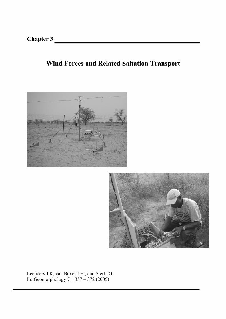
Chapter 3
Wind Forces and Related Saltation Transport
Leenders J.K, van Boxel J.H., and Sterk, G. In: Geomorphology 71: 357 – 372 (2005)

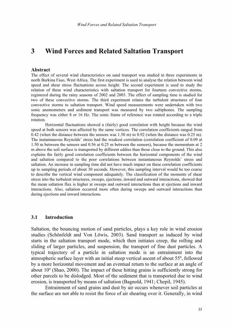
Wind Forces and Related Saltation Transport
35
3 Wind Forces and Related Saltation Transport Abstract The effect of several wind characteristics on sand transport was studied in three experiments in north Burkina Faso, West Africa. The first experiment is used to analyse the relation between wind speed and shear stress fluctuations across height. The second experiment is used to study the relation of these wind characteristics with saltation transport for fourteen convective storms, registered during the rainy seasons of 2002 and 2003. The effect of sampling time is studied for two of these convective storms. The third experiment relates the turbulent structures of four convective storms to saltation transport. Wind speed measurements were undertaken with two sonic anemometers and sediment transport was measured by two saltiphones. The sampling frequency was either 8 or 16 Hz. The sonic frame of reference was rotated according to a triple rotation. Horizontal fluctuations showed a (fairly) good correlation with height because the wind speed at both sensors was affected by the same vortices. The correlation coefficients ranged from 0.42 (when the distance between the sensors was 1.50 m) to 0.92 (when the distance was 0.25 m). The instantaneous Reynolds’ stress had the weakest correlation (correlation coefficient of 0.09 at 1.50 m between the sensors and 0.56 at 0.25 m between the sensors), because the momentum at 2 m above the soil surface is transported by different eddies than those close to the ground. This also explains the fairly good correlation coefficients between the horizontal components of the wind and saltation compared to the poor correlations between instantaneous Reynolds’ stress and saltation. An increase in sampling time did not have much impact on these correlation coefficients up to sampling periods of about 30 seconds. However, this sampling interval would be too coarse to describe the vertical wind component adequately. The classification of the moments of shear stress into the turbulent structures, sweeps, ejections, inward and outward interactions, showed that the mean saltation flux is higher at sweeps and outward interactions than at ejections and inward interactions. Also, saltation occurred more often during sweeps and outward interactions than during ejections and inward interactions. 3.1 Introduction Saltation, the bouncing motion of sand particles, plays a key role in wind erosion studies (Schönfeldt and Von Löwis, 2003). Sand transport as induced by wind starts in the saltation transport mode, which then initiates creep, the rolling and sliding of larger particles, and suspension, the transport of fine dust particles. A typical trajectory of a particle in saltation mode is an entrainment into the atmospheric surface layer with an initial steep vertical ascent of about 55º, followed by a more horizontal movement and an eventual return to the surface at an angle of about 10º (Shao, 2000). The impact of these hitting grains is sufficiently strong for other parcels to be dislodged. Most of the sediment that is transported due to wind erosion, is transported by means of saltation (Bagnold, 1941; Chepil, 1945). Entrainment of sand grains and dust by air occurs whenever soil particles at the surface are not able to resist the force of air shearing over it. Generally, in wind
Chapter 3
36
erosion studies, the driving force for saltation is considered to be the streamwise shear stress (Bagnold, 1941; Chepil and Woodruff, 1963; Wilson and Cooke, 1980; Shao, 2000). This stress results from the transfer of horizontal momentum from the atmosphere to the soil surface, and is only significant when the fluid is in turbulent motion. For airflow this is always the case as the flow depth in the atmosphere is relatively large and the viscosity of air is low. Usually the shear stress is quantified by friction velocity, one of the main scaling parameters in similarity theory of the atmospheric boundary layer (Stull, 1988). Recently, there has been some debate on the driving force of saltation. Sterk et al. (1998) stated that it is not the streamwise shear stress component, but the horizontal drag that is the driving force for saltation. This statement was based on fairly good correlations between moments of saltation transport and fluctuations in horizontal wind speed, compared to poor correlations between moments of saltation transport and instantaneous shear stress. Earlier, Heathershaw and Thorne (1985) drew the same conclusion for the movement of sediment in tidal currents. Although the results of Sterk et al. (1998) can be criticised on the equipment and low sampling frequency, Schönfeldt and Von Löwis (2003) substantiated the results, using higher sampling frequencies and equipment with a faster response time. In most practical wind erosion studies an indirect quantification (or surrogate) of shear stress is used. Often, the average momentum flux, known as the friction velocity, is derived from the profile of the mean wind. This method is based on an important feature of the atmospheric surface layer, namely a constant shear stress layer within it (Shao, 2000). In order to obtain sound values of the average horizontal momentum flux, or friction velocity, the measurement period needs to be sufficiently long to contain at least some of the largest eddies. However, if the measurement period is too long, the trends resulting from the daily course will start influencing the results. Van Boxel et al. (2004) recommended a measuring interval of about 20 minutes when the sensors are placed up to 2.0 m from the surface. In some wind erosion studies, the instantaneous momentum flux at a certain position in the atmospheric boundary layer can be measured directly. In those studies equipment such as a sonic anemometer, is used to measure the wind vector accurately at a high sample rate. Van Boxel et al. (2004) used sonic anemometers to determine correlations between instantaneous shear stress measured at different heights between 0.2 and 2.0 m above the surface. It was shown that at a certain moment the instantaneous shear stress at some height above the surface is not representative for the instantaneous shear stress near the surface. The momentum transported at a couple of metres above the soil surface at a specific time is transported by different vortices than those very close to the surface. This means that the instantaneous shear stress at the soil surface, that is supposed to initiate particle transport, cannot be determined with sonic anemometers. Even though the measured shear stresses were based on runs of five minutes, which is rather short to obtain sound values of shear stress (Van Boxel et al., 2004), these results create at least some doubt that
Wind Forces and Related Saltation Transport
37
the streamwise shear stress component is not the driving force for sediment transport as made by Sterk et al. (1998) and Heathershaw and Thorne (1985). In most sand-transport equations (e.g. Bagnold, 1937; Zingg, 1953; Kawamura, 1964; Owen, 1964; Lettau and Lettau, 1978; White, 1979; Anderson and Haff, 1991; Shao and Li, 1999) the streamwise saltation flux is expressed as a function of the friction velocity and threshold friction velocity. The threshold friction velocity is the minimum friction velocity required for the aerodynamic forces to overcome the retarding forces of the surface (Shao, 2000). Each of these transport equations attempts to quantify the amount of sediment transport in a certain area. They are not very suitable for obtaining insight into the moments that sediment transport actually occurs. For this, sediment transport should be modelled at short time steps, of e.g. several seconds or one minute. However, these intervals are too short to obtain correct values of friction velocity (Van Boxel et al., 2004). Therefore, it might be worthwhile considering the use of other parameters instead of friction velocity to improve the current sand transport equations. Sterk et al. (1998) suggested exploring the possibility of the drag force for this purpose. The aim of this paper is to provide more insight into the relationship between turbulent air flow and related saltation transport. In addition it examines which parameter - shear stress or drag force - would be best for modelling purposes on small timescales. 3.2 Theoretical background The wind vector above a surface can be described by three orthogonal components (u, v and w). In a streamline coordinate system the x-axis (u-component) is oriented into the mean local wind direction, the z-axis (w-component) is orthogonal to x, perpendicular to and up from the plane of the local terrain and the y-axis (v-component) lies in the plane of the local terrain in such a direction that a right-handed coordinate system results (Wilczak et al., 2000). Each component of this wind vector can then be split by Reynolds averaging (Reynolds, 1895) into a mean part (denoted by an overline) and a fluctuating part (denoted by a prime): 'uuu += ;
'vvv += and 'www += . The fluctuating components (u’, v’ and w’) cause shear stress in the fluid. The total stress exerted by the turbulent fluid flow is described by the Reynolds’ stress (RS) tensor, which consists of nine stress components. The shear stress at a solid boundary is equal to the average vertical flux of horizontal momentum measured near the surface. This is expressed by two parameters of the RS-tensor:
''wuxz ρτ −= and ''wvyz ρτ −= , in which xzτ is the vertical flux of momentum in the x-direction and yzτ the vertical flux of momentum in the y-direction; ρ is the density of the fluid; u’, v’ and w’ are the perturbation values of wind speed in the x-, y- and z- plane respectively. Friction velocity is defined by ρτ Ru ≡2
* , in which
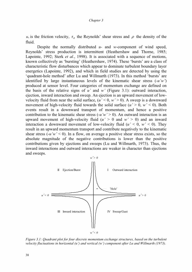
Chapter 3
38
*u is the friction velocity, Rτ the Reynolds’ shear stress and ρ the density of the fluid. Despite the normally distributed u- and w-component of wind speed, Reynolds’ stress production is intermittent (Heathershaw and Thorne, 1985; Lapointe, 1992; Sterk et al., 1998). It is associated with a sequence of motions, known collectively as ‘bursting’ (Heathershaw, 1974). These ‘bursts’ are a class of characteristic flow disturbances which appear to dominate turbulent boundary layer energetics (Lapointe, 1992), and which in field studies are detected by using the ‘quadrant-hole method’ after Lu and Willmarth (1973). In this method ‘bursts’ are identified by large instantaneous levels of the kinematic shear stress (-u’w’) produced at sensor level. Four categories of momentum exchange are defined on the basis of the relative signs of u’ and w’ (Figure 3.1): outward interaction, ejection, inward interaction and sweep. An ejection is an upward movement of low-velocity fluid from near the solid surface, (u’ < 0, w’ > 0). A sweep is a downward movement of high-velocity fluid towards the solid surface (u’ > 0, w’ < 0). Both events result in a downward transport of momentum, and hence a positive contribution to the kinematic shear stress (-u’w’ > 0). An outward interaction is an upward movement of high-velocity fluid (u’ > 0 and w’ > 0) and an inward interaction a downward movement of low-velocity fluid (u’ < 0, w’ < 0). They result in an upward momentum transport and contribute negatively to the kinematic shear stress (-u’w’ < 0). In a flow, on average a positive shear stress exists, so the absolute magnitude of the negative contributions is lower than the positive contributions given by ejections and sweeps (Lu and Willmarth, 1973). Thus, the inward interactions and outward interactions are weaker in character than ejections and sweeps.
w′ > 0
w′ < 0
u′ > 0 u′ < 0
I II
III IV
Outward interaction Ejection/Burst
Inward interaction Sweep/Gust
′Hole′
Figure 3.1: Quadrant plot for four discrete momentum exchange structures, based on the turbulent velocity fluctuations in horizontal (u’) and vertical (w’) component after Lu and Willmarth (1973).
Wind Forces and Related Saltation Transport
39
The ‘hole’ of the ‘quadrant-hole’ technique refers to the exclusion of values of kinematic stress less than some threshold H, to distinguish true ‘bursts’ from weaker background events (Lapointe, 1992). Only those events that exceeded the average kinematic stress by threshold, H, are identified as structures, the instantaneous values in the interval of [ HwuHwu +−−− '','' ] are not considered as a turbulent structure. The vexed question is what constitutes a proper threshold, H, to identify an event (Lapointe, 1992). Willmarth and Lu (1974) used an event threshold of 10 times the mean stress, based on the disappearance of sweep events above this threshold far from the wall in a flume. Bogard and Tiederman (1986), who worked much closer to the boundary, recommended a threshold roughly 2-3 times mean stress. Gordon (1974), working with large scale flows, used a threshold equal to twice the median value of -u’w’. Finally, Sterk et al. (1998) used one standard deviation of -u’w’ as a threshold value. Few studies that are based on field experiments, have tried to relate the structures of Reynolds’ shear stress in the boundary layer to sediment transport. The major drawback was the resolution time of sediment transport measurements. One of the first of these studies dealt with bed load transport at the sea bed (Heathershaw and Thorne, 1985). The results showed that bed-load movement of sea-bed gravels was caused principally by sweep-type motions in the bottom boundary layer and to a lesser extent by outward interactions. In a different study, it was found that suspended load transport of finer sediments in a river was dominated by ejection-type events (Lapointe, 1992). Sterk et al. (1998) were the first who tried to relate turbulent structures to wind-blown saltation transport. Their results were consistent with the results of Heathershaw and Thorne (1985), and showed that saltation transport was mainly occurring during sweeps and outward interactions, while saltation transport was almost negligible during ejections and inward interactions. These results were later substantiated by Schönfeldt and Von Löwis (2003), who used a higher sampling frequency than Sterk et al. (1998). 3.3 Materials and Methods 3.3.1 Study site The experiment was carried out on a farmer’s field 7 km south east of Dori, the capital of Seno province in north Burkina Faso, during the rainy seasons of 2002 and 2003. The climate of the region is typical Sahelian with a rainy season from May to September and high temperatures throughout the year. The average annual rainfall in the area is 420 mm, but both seasons of 2002 and 2003 deviated from average; in 2002 the measured total amount of rainfall was 350 mm, in 2003 this was 1050 mm. At the start of the rainy season, large cumulonimbus clouds that bring the first rains develop throughout the Sahel. These clouds are often accompanied by short wind storms, lasting 10 to 30 minutes, preceding rainfall. The storms are the
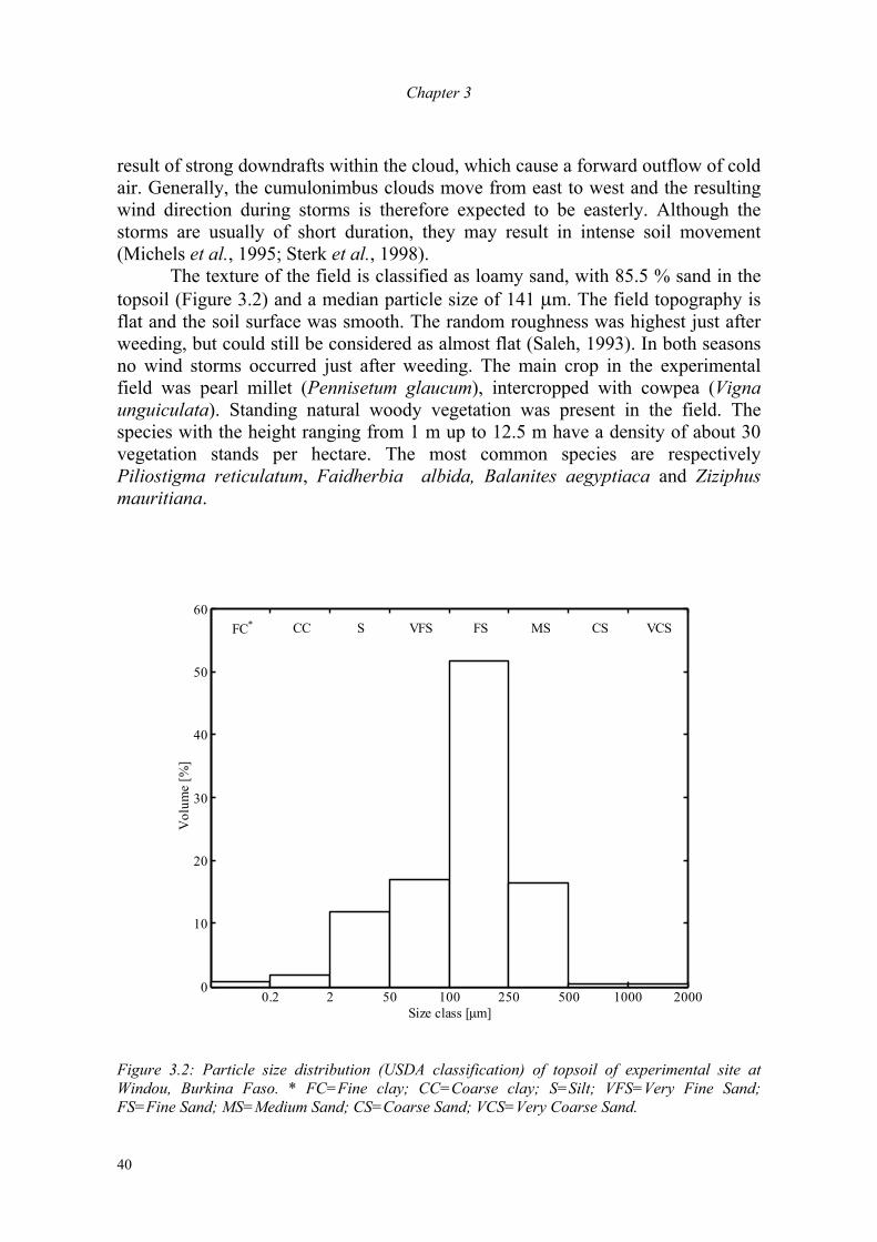
Chapter 3
40
result of strong downdrafts within the cloud, which cause a forward outflow of cold air. Generally, the cumulonimbus clouds move from east to west and the resulting wind direction during storms is therefore expected to be easterly. Although the storms are usually of short duration, they may result in intense soil movement (Michels et al., 1995; Sterk et al., 1998). The texture of the field is classified as loamy sand, with 85.5 % sand in the topsoil (Figure 3.2) and a median particle size of 141 µm. The field topography is flat and the soil surface was smooth. The random roughness was highest just after weeding, but could still be considered as almost flat (Saleh, 1993). In both seasons no wind storms occurred just after weeding. The main crop in the experimental field was pearl millet (Pennisetum glaucum), intercropped with cowpea (Vigna unguiculata). Standing natural woody vegetation was present in the field. The species with the height ranging from 1 m up to 12.5 m have a density of about 30 vegetation stands per hectare. The most common species are respectively Piliostigma reticulatum, Faidherbia albida, Balanites aegyptiaca and Ziziphus mauritiana.
0.2 2 50 100 250 500 1000 20000
10
20
30
40
50
60
Size class [µm]
Vol
ume
[%]
FC* CC S VFS FS MS CS VCS
Figure 3.2: Particle size distribution (USDA classification) of topsoil of experimental site at Windou, Burkina Faso. * FC=Fine clay; CC=Coarse clay; S=Silt; VFS=Very Fine Sand; FS=Fine Sand; MS=Medium Sand; CS=Coarse Sand; VCS=Very Coarse Sand.
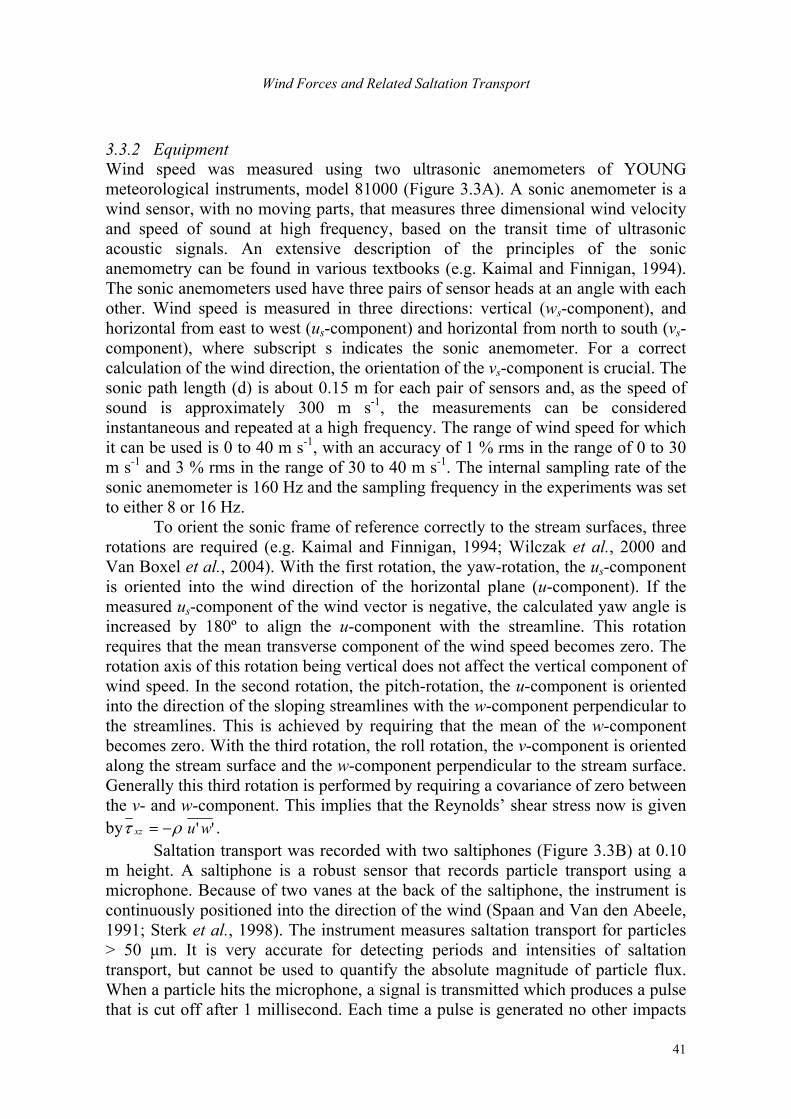
Wind Forces and Related Saltation Transport
41
3.3.2 Equipment Wind speed was measured using two ultrasonic anemometers of YOUNG meteorological instruments, model 81000 (Figure 3.3A). A sonic anemometer is a wind sensor, with no moving parts, that measures three dimensional wind velocity and speed of sound at high frequency, based on the transit time of ultrasonic acoustic signals. An extensive description of the principles of the sonic anemometry can be found in various textbooks (e.g. Kaimal and Finnigan, 1994). The sonic anemometers used have three pairs of sensor heads at an angle with each other. Wind speed is measured in three directions: vertical (ws-component), and horizontal from east to west (us-component) and horizontal from north to south (vs-component), where subscript s indicates the sonic anemometer. For a correct calculation of the wind direction, the orientation of the vs-component is crucial. The sonic path length (d) is about 0.15 m for each pair of sensors and, as the speed of sound is approximately 300 m s-1, the measurements can be considered instantaneous and repeated at a high frequency. The range of wind speed for which it can be used is 0 to 40 m s-1, with an accuracy of 1 % rms in the range of 0 to 30 m s-1 and 3 % rms in the range of 30 to 40 m s-1. The internal sampling rate of the sonic anemometer is 160 Hz and the sampling frequency in the experiments was set to either 8 or 16 Hz. To orient the sonic frame of reference correctly to the stream surfaces, three rotations are required (e.g. Kaimal and Finnigan, 1994; Wilczak et al., 2000 and Van Boxel et al., 2004). With the first rotation, the yaw-rotation, the us-component is oriented into the wind direction of the horizontal plane (u-component). If the measured us-component of the wind vector is negative, the calculated yaw angle is increased by 180º to align the u-component with the streamline. This rotation requires that the mean transverse component of the wind speed becomes zero. The rotation axis of this rotation being vertical does not affect the vertical component of wind speed. In the second rotation, the pitch-rotation, the u-component is oriented into the direction of the sloping streamlines with the w-component perpendicular to the streamlines. This is achieved by requiring that the mean of the w-component becomes zero. With the third rotation, the roll rotation, the v-component is oriented along the stream surface and the w-component perpendicular to the stream surface. Generally this third rotation is performed by requiring a covariance of zero between the v- and w-component. This implies that the Reynolds’ shear stress now is given by ''wuxz ρτ −= . Saltation transport was recorded with two saltiphones (Figure 3.3B) at 0.10 m height. A saltiphone is a robust sensor that records particle transport using a microphone. Because of two vanes at the back of the saltiphone, the instrument is continuously positioned into the direction of the wind (Spaan and Van den Abeele, 1991; Sterk et al., 1998). The instrument measures saltation transport for particles > 50 µm. It is very accurate for detecting periods and intensities of saltation transport, but cannot be used to quantify the absolute magnitude of particle flux. When a particle hits the microphone, a signal is transmitted which produces a pulse that is cut off after 1 millisecond. Each time a pulse is generated no other impacts
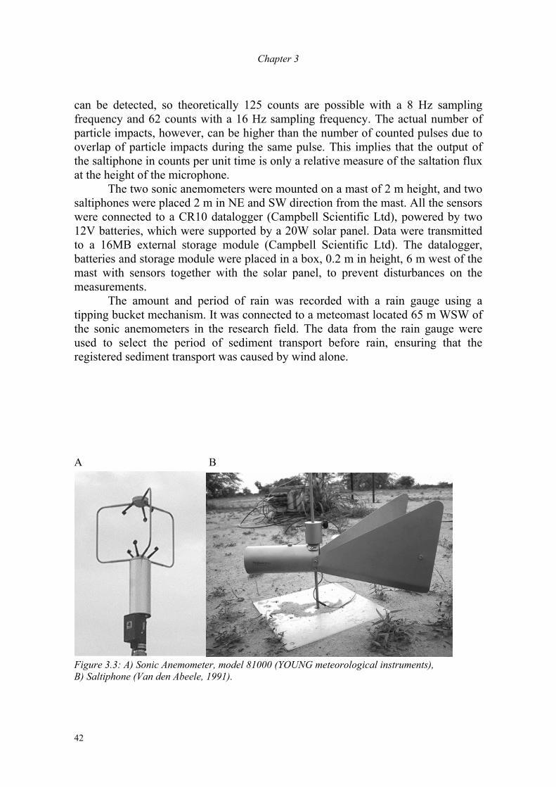
Chapter 3
42
can be detected, so theoretically 125 counts are possible with a 8 Hz sampling frequency and 62 counts with a 16 Hz sampling frequency. The actual number of particle impacts, however, can be higher than the number of counted pulses due to overlap of particle impacts during the same pulse. This implies that the output of the saltiphone in counts per unit time is only a relative measure of the saltation flux at the height of the microphone. The two sonic anemometers were mounted on a mast of 2 m height, and two saltiphones were placed 2 m in NE and SW direction from the mast. All the sensors were connected to a CR10 datalogger (Campbell Scientific Ltd), powered by two 12V batteries, which were supported by a 20W solar panel. Data were transmitted to a 16MB external storage module (Campbell Scientific Ltd). The datalogger, batteries and storage module were placed in a box, 0.2 m in height, 6 m west of the mast with sensors together with the solar panel, to prevent disturbances on the measurements. The amount and period of rain was recorded with a rain gauge using a tipping bucket mechanism. It was connected to a meteomast located 65 m WSW of the sonic anemometers in the research field. The data from the rain gauge were used to select the period of sediment transport before rain, ensuring that the registered sediment transport was caused by wind alone. A B
Figure 3.3: A) Sonic Anemometer, model 81000 (YOUNG meteorological instruments), B) Saltiphone (Van den Abeele, 1991).
Wind Forces and Related Saltation Transport
43
3.3.3 Experiment 1 The first experiment was set up to determine the relation between the u- and w-component of wind speed and the instantaneous RS across height. Wind measurements were undertaken with the two sonic anemometers placed at different heights on the mast. One of the sonic anemometers was always positioned on top of the mast, with the centre of the sonic path at 2 m height. The other was placed on an arm of 0.5 m length, which was attached to the mast, oriented to the east and adjustable in height. The experiment consisted of seven runs with a sampling period of 30 minutes and a sampling rate of 8 Hz. The measurements were made with the centre of the second sonic at 0.25 m, 0.50 m, 0.75 m, 1.00 m, 1.25 m, 1.50 m and 1.75 m height. The sampling period of 30 minutes is statistically long enough to contain at least a few of the largest eddies (Stull, 1988; Van Boxel et al., 2004). The mean wind vector and direction of this experiment were calculated over the whole record of 30 minutes. The instantaneous us-, vs- and ws-velocity components of each run were converted to the components of u, v and w by performing a triple rotation of the coordinate axes (e.g. Kaimal and Finnigan, 1994; Wilczak et al., 2000; Van Boxel et al., 2004). The u- and w-components were subsequently used to calculate the instantaneous values of shear stress. Finally, the correlation coefficients between the components of u and w and instantaneous shear stress across height were calculated. 3.3.4 Experiment 2 A second experiment was set up to determine the relation between saltation transport and fluctuations in wind speed and shear stress and to study the effect of sampling frequency. For this experiment the sonic anemometers were installed with the centre at 1 m and 2 m above the soil surface. Two saltiphones were placed 2 m in NE and SW direction from the mast with the sonic anemometers, with the microphone at 0.10 m above the soil surface. The sampling frequency of the sonic anemometers and the saltiphones was set to 8 Hz in 2002. In 2003 the sampling frequency was increased to 16 Hz to enable a more detailed recording of fluctuations. In this setup the station was programmed so that the sonic anemometers started to measure, when the saltiphones registered a particle transport of ≥ 40 hits per second. If the saltiphones registered a particle transport of ≤ 24 hits per second during 5 minutes, the sonic anemometers were turned off automatically. The average windvector and direction were calculated for the duration of the event. The start of an event was a registration of ≥ 40 hits per second by the saltiphones. The end was marked by either a registration of the saltiphones of ≤ 24 hits per second, or by the moment that it started to rain, which immediately stopped all saltation transport. For each event the instantaneous us-, vs- and ws-velocity components were converted to the components of u, v and w by performing a triple
Chapter 3
44
rotation of the coordinate axes (e.g. Kaimal and Finnigan, 1994; Wilczak et al., 2000; Van Boxel et al., 2004). Subsequently the instantaneous RS was calculated and together with the values of u and w related to the measured saltation flux. The effect of sampling time was studied for the event with the longest duration of each year. The direct output of the sonic anemometers was averaged to simulate the effect of lower sampling frequencies. In 2002, the simulated sampling frequencies were 4 Hz, 2 Hz, 1 Hz, 2 sec, 4 sec, 8 sec, 16 sec, 30 sec, 60 sec and 2 min. For 2003, the same frequencies were simulated, extended with the frequency of 8 Hz. The averaged us-, vs- and ws-velocity components were transformed to new u-, v- and w- velocity components with a triple rotation of the coordinate system (Kaimal and Finnigan, 1994; Wilczak et al., 2000; Van Boxel et al., 2004). Finally, correlations between the saltation flux and the u-component, w-component and instantaneous RS were calculated. 3.3.5 Experiment 3 A third experiment was used to relate saltation transport to turbulent structures. For this experiment the same experimental setup was used as for experiment 2. For both experimental seasons two events were selected for the analysis of this experiment; one with a low frequent saltation transport, and one with a high frequent saltation transport. For each of these events, the categories of momentum exchange were defined on the relative signs of the perturbation values of the u- and w-component, according to the ‘quadrant-hole method’ of Lu and Willmarth (1973) (Figure 3.1). The threshold to distinguish a turbulent structure from the weaker background was set to the standard deviation of the kinematic stress (Sterk et al., 1998). 3.4 Results 3.4.1 Experiment 1 The experiment was carried out on the 2nd of July and the 7th of August in 2002. The average temperatures during the experiment were 32.9º C (σ = 2.4º C) and 31.8º C (σ = 1.7º C) respectively. The average wind velocity at 2 m on 2 July 2002 was 5.3 m s-1 (σ = 1.2 m s-1), with a direction of 247º (σ = 16º). On 7 August 2002 the average wind speed was 2.8 m s-1 (σ = 1.0 m s-1) with a direction of 196º (σ = 23º). For each run, the u-component of both sensors showed the best correlation, compared to the w-component and instantaneous shear stress (Figure 3.4). The RS showed the poorest correlation with height. As the distance between the sensors increased, the strength of correlation decreased. At a large distance between the sensors, the values deviate slightly, as one of the sonic anemometers is positioned very close to the surface. For the u-component on 2 July 2002, the correlation
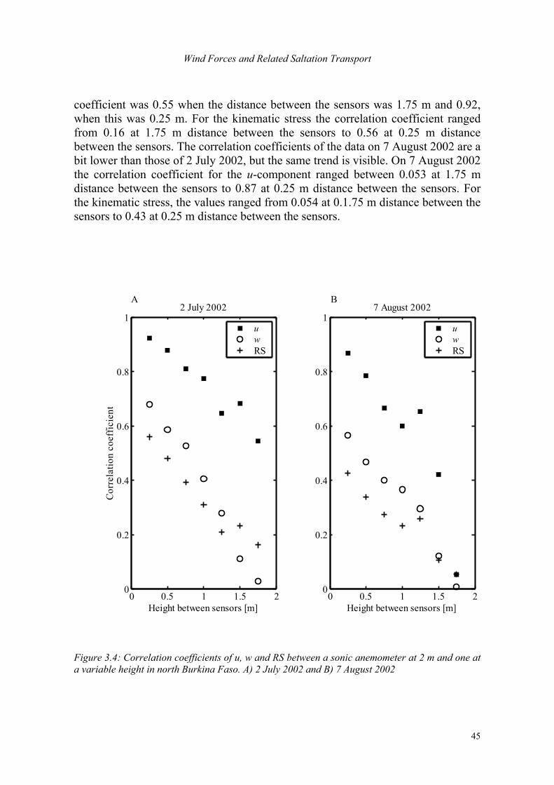
Wind Forces and Related Saltation Transport
45
coefficient was 0.55 when the distance between the sensors was 1.75 m and 0.92, when this was 0.25 m. For the kinematic stress the correlation coefficient ranged from 0.16 at 1.75 m distance between the sensors to 0.56 at 0.25 m distance between the sensors. The correlation coefficients of the data on 7 August 2002 are a bit lower than those of 2 July 2002, but the same trend is visible. On 7 August 2002 the correlation coefficient for the u-component ranged between 0.053 at 1.75 m distance between the sensors to 0.87 at 0.25 m distance between the sensors. For the kinematic stress, the values ranged from 0.054 at 0.1.75 m distance between the sensors to 0.43 at 0.25 m distance between the sensors.
0 0.5 1 1.5 20
0.2
0.4
0.6
0.8
12 July 2002
Height between sensors [m]
Corr
elat
ion
coef
ficie
nt
uwRS
0 0.5 1 1.5 20
0.2
0.4
0.6
0.8
17 August 2002
Height between sensors [m]
uwRS
A B
Figure 3.4: Correlation coefficients of u, w and RS between a sonic anemometer at 2 m and one at a variable height in north Burkina Faso. A) 2 July 2002 and B) 7 August 2002
Chapter 3
46
These values are in correspondence with those that were found by Van Boxel et al. (2004). The much better cross-correlation with height for the horizontal wind component than for the vertical component can be explained by the type of vortices that contribute to the different wind components. Large vortices, with low frequencies contribute much to fluctuations in the horizontal wind speed. These vortices have relatively long lifetimes and the vortex that causes a fluctuation in the wind speed at 2 m height will also affect the wind speed at lower heights. The vortices that contribute most to the vertical fluctuations have sizes in the order of the observation height, which means that the vertical wind speed fluctuations near the ground, are caused by different eddies that those at 2 m height. This implies that the instantaneous RS at the soil surface, the stress that causes entrainment of soil particles, is not well registered at several metres above the soil surface. Therefore a high correlation between instantaneous RS as measured at some distance from the soil surface and saltation transport is not to be expected. 3.4.2 Experiment 2 During the two measuring campaigns, a total of 28 events with sand transport occurred, 18 in 2002 and 10 in 2003. Some of these events were of very low intensity and lasted only a few minutes. For the year 2002, complete records of events were only recorded for the month of June because of malfunctioning of the station in the other months. In total, data from 14 storms (6 in 2002 and 8 in 2003) were obtained for use in the analysis of this paper. In Table 3.1A and 3.1B the general wind characteristics at 2 m height of these storms are summarised, together with the data of one of the saltiphones. There is a large variety among the events. Half of the events, e.g. those of 4 June 2002 and 15 May 2003, were actually followed by rain. This was not related to the direction of the storm; the events of both 4 June 2003 and 13 July 2003 came from the same direction and only the event of 13 July 2003 was followed by rainfall. The duration of the events varied from less than 10 minutes up to one and a half hours. This duration was not related to the intensity of saltation. The event of 13 July 2003, for example, had an intense saltation transport during 8.2 minutes and on 14 June 2002 there was intense saltation transport for more than an hour. The average wind speed of the storms ranged from 7.4 m s-1 up to 12.2 m s-1. What is striking is that the last four events in 2003, recorded a higher average wind velocity than the first four events that were recorded in 2003. This is explained by the pearl millet, which was sown the 27th of May 2003 that protected the soil surface increasing its resistance for wind erosion. In these circumstances, higher wind velocities are necessary than at the start of the season, for wind erosion to occur. The direction of the storms ranged from NNE (23º on 21 May 2003) to SSW (191º on 15 May 2003). Also, within a storm a wide range of wind direction existed.
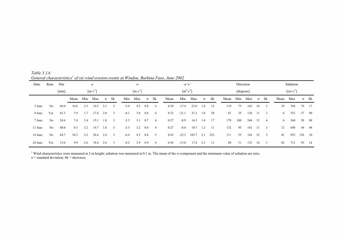
Table 3.1A: General characteristics1 of six wind erosion events at Windou, Burkina Faso, June 2002
Date Rain Dur u w -u’w’ Direction Saltation
[min] [m s-1] [m s-1] [m2 s-2] [degrees] [cts s-1]
Mean Min Max σ Sk Min Max σ Sk Mean Min Max σ Sk Mean Min Max σ Sk Mean Max σ Sk
3 June No 69.0 10.6 3.5 19.5 2.3 3 -3.9 4.5 0.8 4 0.39 -17.4 22.0 1.8 15 119 75 163 10 3 39 768 79 17
4 June Yes 43.3 7.9 1.7 17.6 2.0 3 -4.1 3.8 0.8 4 0.32 -21.1 31.2 1.8 28 81 35 126 11 3 6 552 27 90
7 June No 24.6 7.4 2.4 15.1 1.8 3 -3.3 3.1 0.7 4 0.27 -8.9 16.3 1.4 17 178 100 244 13 4 4 360 20 88
11 June No 40.0 8.3 3.2 14.7 1.8 3 -3.3 3.2 0.6 4 0.27 -8.8 10.7 1.2 11 132 95 181 11 3 12 640 44 48
14 June No 64.7 10.3 3.2 26.6 2.4 3 -6.4 4.5 0.8 5 0.43 -32.3 103.7 2.1 223 111 55 164 12 3 81 952 156 10
24 June Yes 13.6 9.9 2.6 18.4 2.6 3 -4.2 3.9 0.9 4 0.56 -15.8 17.4 2.3 11 88 31 132 14 3 42 712 95 14
1 Wind characteristics were measured at 2 m height; saltation was measured at 0.1 m. The mean of the w-component and the minimum value of saltation are zero. σ = standard deviation; Sk = skewness
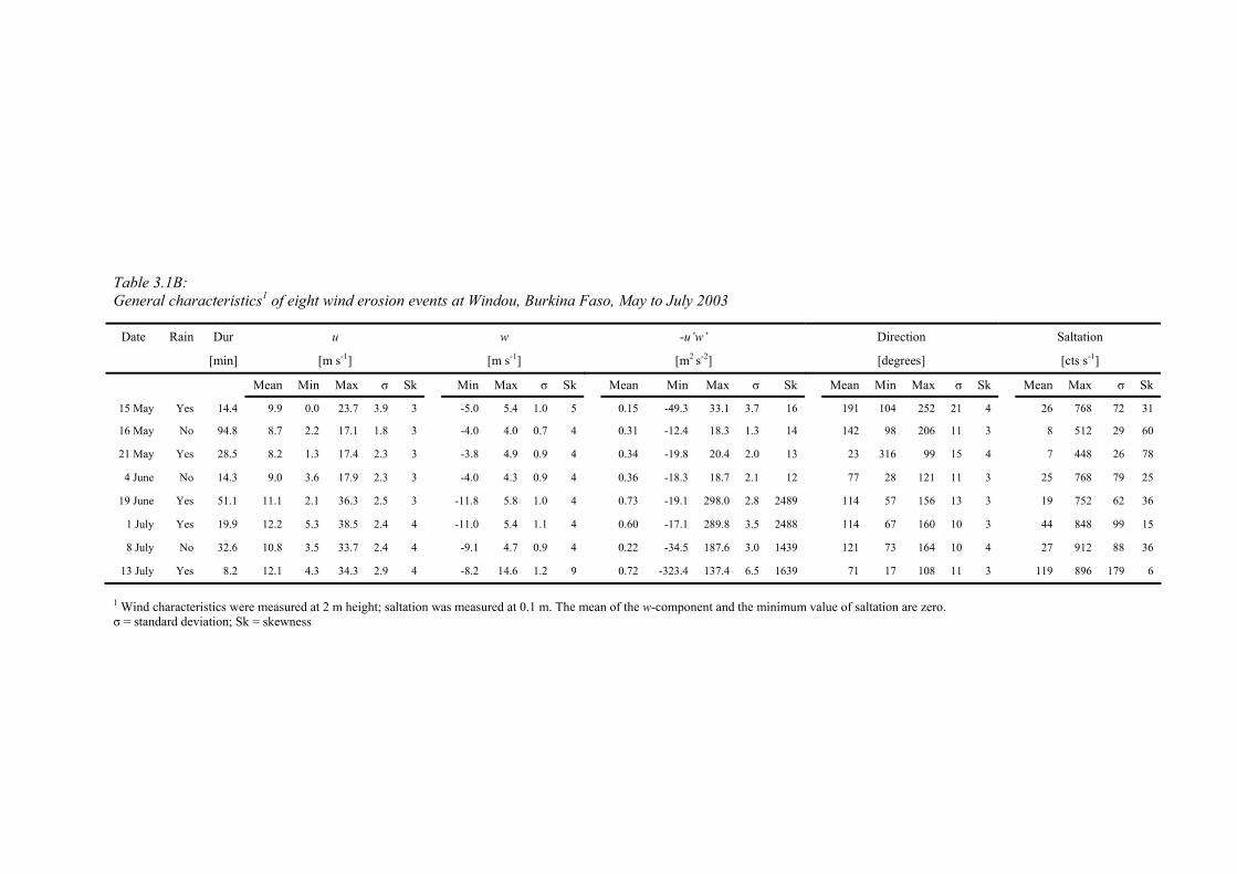
Table 3.1B: General characteristics1 of eight wind erosion events at Windou, Burkina Faso, May to July 2003
Date Rain Dur u w -u’w’ Direction Saltation
[min] [m s-1] [m s-1] [m2 s-2] [degrees] [cts s-1]
Mean Min Max σ Sk Min Max σ Sk Mean Min Max σ Sk Mean Min Max σ Sk Mean Max σ Sk
15 May Yes 14.4 9.9 0.0 23.7 3.9 3 -5.0 5.4 1.0 5 0.15 -49.3 33.1 3.7 16 191 104 252 21 4 26 768 72 31
16 May No 94.8 8.7 2.2 17.1 1.8 3 -4.0 4.0 0.7 4 0.31 -12.4 18.3 1.3 14 142 98 206 11 3 8 512 29 60
21 May Yes 28.5 8.2 1.3 17.4 2.3 3 -3.8 4.9 0.9 4 0.34 -19.8 20.4 2.0 13 23 316 99 15 4 7 448 26 78
4 June No 14.3 9.0 3.6 17.9 2.3 3 -4.0 4.3 0.9 4 0.36 -18.3 18.7 2.1 12 77 28 121 11 3 25 768 79 25
19 June Yes 51.1 11.1 2.1 36.3 2.5 3 -11.8 5.8 1.0 4 0.73 -19.1 298.0 2.8 2489 114 57 156 13 3 19 752 62 36
1 July Yes 19.9 12.2 5.3 38.5 2.4 4 -11.0 5.4 1.1 4 0.60 -17.1 289.8 3.5 2488 114 67 160 10 3 44 848 99 15
8 July No 32.6 10.8 3.5 33.7 2.4 4 -9.1 4.7 0.9 4 0.22 -34.5 187.6 3.0 1439 121 73 164 10 4 27 912 88 36
13 July Yes 8.2 12.1 4.3 34.3 2.9 4 -8.2 14.6 1.2 9 0.72 -323.4 137.4 6.5 1639 71 17 108 11 3 119 896 179 6
1 Wind characteristics were measured at 2 m height; saltation was measured at 0.1 m. The mean of the w-component and the minimum value of saltation are zero. σ = standard deviation; Sk = skewness
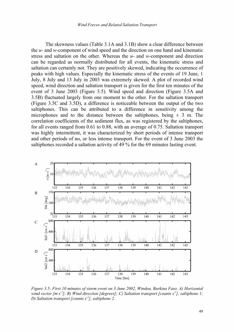
Wind Forces and Related Saltation Transport
49
The skewness values (Table 3.1A and 3.1B) show a clear difference between the u- and w-component of wind speed and the direction on one hand and kinematic stress and saltation on the other. Whereas the u- and w-component and direction can be regarded as normally distributed for all events, the kinematic stress and saltation can certainly not. They are positively skewed, indicating the occurrence of peaks with high values. Especially the kinematic stress of the events of 19 June, 1 July, 8 July and 13 July in 2003 was extremely skewed. A plot of recorded wind speed, wind direction and saltation transport is given for the first ten minutes of the event of 3 June 2003 (Figure 3.5). Wind speed and direction (Figure 3.5A and 3.5B) fluctuated largely from one moment to the other. For the saltation transport (Figure 3.5C and 3.5D), a difference is noticeable between the output of the two saltiphones. This can be attributed to a difference in sensitivity among the microphones and to the distance between the saltiphones, being ± 3 m. The correlation coefficients of the sediment flux, as was registered by the saltiphones, for all events ranged from 0.61 to 0.88, with an average of 0.75. Saltation transport was highly intermittent, it was characterized by short periods of intense transport and other periods of no, or less intense transport. For the event of 3 June 2003 the saltiphones recorded a saltation activity of 49 % for the 69 minutes lasting event.
133 134 135 136 137 138 139 140 141 142 143
10
20
u [m
s-1]
133 134 135 136 137 138 139 140 141 142 14350
100
150
Dir
[deg
]
133 134 135 136 137 138 139 140 141 142 143
400
800
Sal1
[cts
s-1]
133 134 135 136 137 138 139 140 141 142 143
400
800
Sal2
[cts
s-1]
Time [hm]
A
B
C
D
Figure 3.5: First 10 minutes of storm event on 3 June 2002, Windou, Burkina Faso. A) Horizontal wind vector [m s-1]; B) Wind direction [degrees]; C) Saltation transport [counts s-1], saltiphone 1; D) Saltation transport [counts s-1], saltiphone 2.
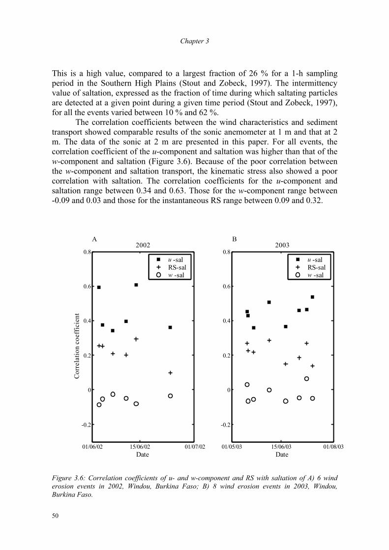
Chapter 3
50
This is a high value, compared to a largest fraction of 26 % for a 1-h sampling period in the Southern High Plains (Stout and Zobeck, 1997). The intermittency value of saltation, expressed as the fraction of time during which saltating particles are detected at a given point during a given time period (Stout and Zobeck, 1997), for all the events varied between 10 % and 62 %.
The correlation coefficients between the wind characteristics and sediment transport showed comparable results of the sonic anemometer at 1 m and that at 2 m. The data of the sonic at 2 m are presented in this paper. For all events, the correlation coefficient of the u-component and saltation was higher than that of the w-component and saltation (Figure 3.6). Because of the poor correlation between the w-component and saltation transport, the kinematic stress also showed a poor correlation with saltation. The correlation coefficients for the u-component and saltation range between 0.34 and 0.63. Those for the w-component range between -0.09 and 0.03 and those for the instantaneous RS range between 0.09 and 0.32.
01/06/02 15/06/02 01/07/02
-0.2
0
0.2
0.4
0.6
0.82002
Date
Cor
rela
tion
coef
ficie
nt
u -salRS-salw -sal
01/05/03 15/06/03 01/08/03
-0.2
0
0.2
0.4
0.6
0.82003
Date
u -salRS-salw -sal
A B
Figure 3.6: Correlation coefficients of u- and w-component and RS with saltation of A) 6 wind erosion events in 2002, Windou, Burkina Faso; B) 8 wind erosion events in 2003, Windou, Burkina Faso.
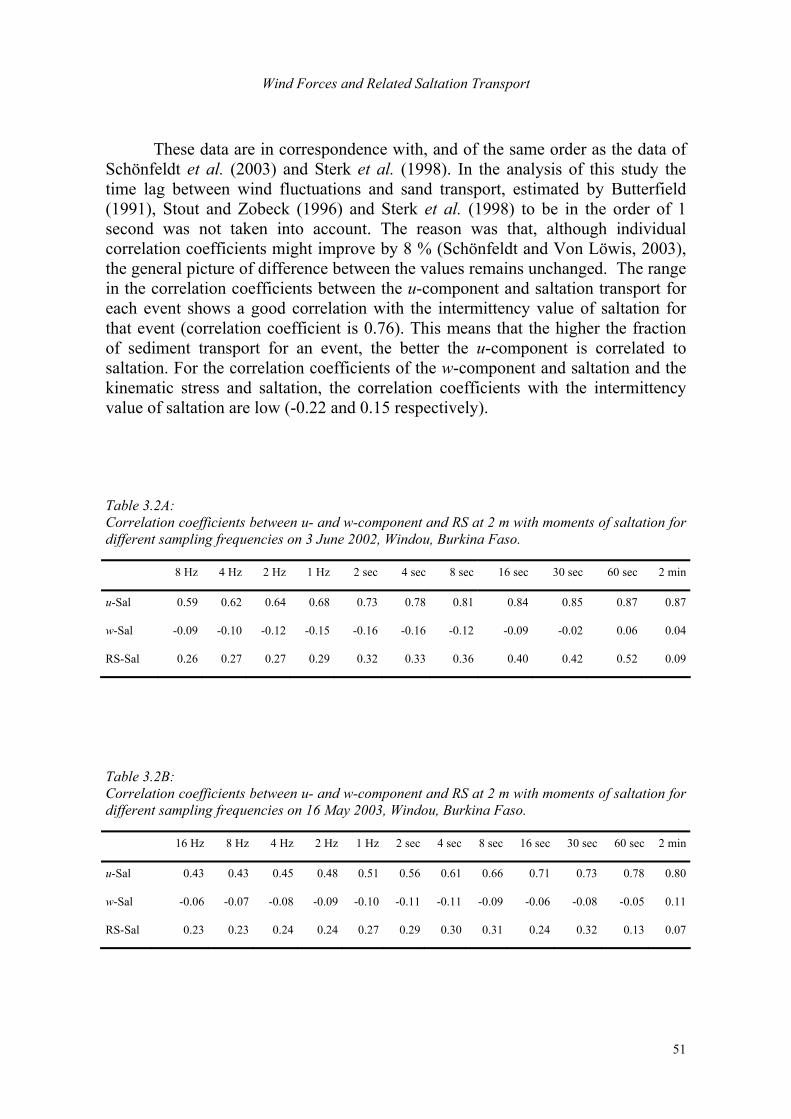
Wind Forces and Related Saltation Transport
51
These data are in correspondence with, and of the same order as the data of Schönfeldt et al. (2003) and Sterk et al. (1998). In the analysis of this study the time lag between wind fluctuations and sand transport, estimated by Butterfield (1991), Stout and Zobeck (1996) and Sterk et al. (1998) to be in the order of 1 second was not taken into account. The reason was that, although individual correlation coefficients might improve by 8 % (Schönfeldt and Von Löwis, 2003), the general picture of difference between the values remains unchanged. The range in the correlation coefficients between the u-component and saltation transport for each event shows a good correlation with the intermittency value of saltation for that event (correlation coefficient is 0.76). This means that the higher the fraction of sediment transport for an event, the better the u-component is correlated to saltation. For the correlation coefficients of the w-component and saltation and the kinematic stress and saltation, the correlation coefficients with the intermittency value of saltation are low (-0.22 and 0.15 respectively). Table 3.2A: Correlation coefficients between u- and w-component and RS at 2 m with moments of saltation for different sampling frequencies on 3 June 2002, Windou, Burkina Faso.
8 Hz 4 Hz 2 Hz 1 Hz 2 sec 4 sec 8 sec 16 sec 30 sec 60 sec 2 min
u-Sal 0.59 0.62 0.64 0.68 0.73 0.78 0.81 0.84 0.85 0.87 0.87
w-Sal -0.09 -0.10 -0.12 -0.15 -0.16 -0.16 -0.12 -0.09 -0.02 0.06 0.04
RS-Sal 0.26 0.27 0.27 0.29 0.32 0.33 0.36 0.40 0.42 0.52 0.09
Table 3.2B: Correlation coefficients between u- and w-component and RS at 2 m with moments of saltation for different sampling frequencies on 16 May 2003, Windou, Burkina Faso.
16 Hz 8 Hz 4 Hz 2 Hz 1 Hz 2 sec 4 sec 8 sec 16 sec 30 sec 60 sec 2 min
u-Sal 0.43 0.43 0.45 0.48 0.51 0.56 0.61 0.66 0.71 0.73 0.78 0.80
w-Sal -0.06 -0.07 -0.08 -0.09 -0.10 -0.11 -0.11 -0.09 -0.06 -0.08 -0.05 0.11
RS-Sal 0.23 0.23 0.24 0.24 0.27 0.29 0.30 0.31 0.24 0.32 0.13 0.07
Chapter 3
52
The events of 3 June 2002 and 16 May 2003 were selected to analyse the effect of sampling time on the correlation coefficients. Due to the long duration of those events, a sufficiently large database is provided to calculate correlation coefficients for longer sampling intervals. The correlation coefficient between the u-component and the moments of saltation remained high and increased with an increase in sampling time (Table 3.2A and 3.2B). The correlation between the w-component and moments of saltation remained low. When the sampling time was in the order of a minute, the correlation of the w-component with saltation changed sign. At this point the sampling interval has become too rough to measure the w-component adequately, and therefore a quantification of the instantaneous value of kinematic stress doesn’t exist anymore. 3.4.3 Experiment 3 In 2002, the events of 3 June and 4 June were selected to analyze the effect of turbulent structures on saltation transport. They had an intermittency level of respectively 0.49 and 0.13. In 2003 it concerned the events of 21 May, with an intermittency level of 0.19 and 13 July, with an intermittency level of 0.65. Table 3.3 summarises some characteristics for each turbulent structure for these events. Of the distinguished turbulent structures, the occurrence of sweeps at both sonic anemometers is the most frequent. The correlation between the structures registered at 1 m and at 2 m is the strongest for the events with a low overall intermittency value of saltation (and a low wind speed); the events of 4 June 2002 and 21 May 2003. During these events, in 19 % of the cases that the sonic at 2 m registered a sweep, the sonic at 1 m also registered a sweep. For the events of 3 June 2002 and 13 July 2003 this value is only 5 %.
Turbulent structures occurred in less than 20 % of the time, but contributed to approximately 60 % of the shear stress. Of the structures, sweeps contributed most to the shear stress. They were the most frequent and their value of mean stress was the highest. After sweeps, the outward interactions were the most frequent, followed by ejections and inward interactions. The calculated duration of a turbulent structure seems very much influenced by the sampling frequency. In this study, the average duration of turbulent structures was estimated to be around 0.2 sec in 2002, when the sampling frequency was 8 Hz and around 0.1 sec with a sampling frequency of 16 Hz. Sterk et al. (1998) found average durations of turbulent structures between 1 and 1.5 seconds. Their sampling frequency was 1 Hz. The difference in average duration is explained by the sampling frequency. Higher sampling frequencies enable a better distinction in moments of high and low kinematic stress, which results in a shortening of the estimated durations of a turbulent structure. Overall, the turbulent structures showed a poor correlation with saltation. This is partly explained because saltation does not occur for a certain period of time. Over this period saltation is constant whereas u’ and w’ vary, resulting in a low correlation. The turbulent structures with a positive u’, sweeps and outward
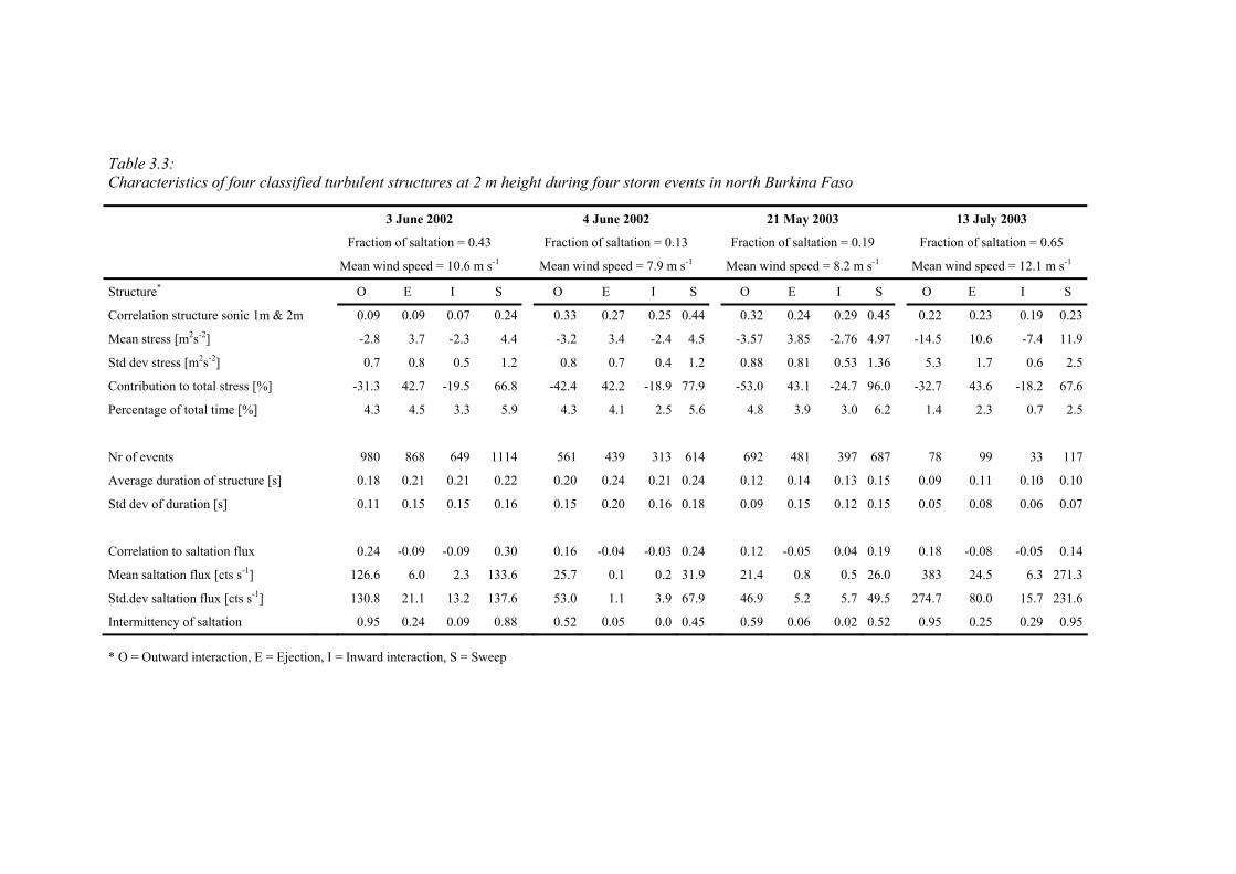
Table 3.3: Characteristics of four classified turbulent structures at 2 m height during four storm events in north Burkina Faso
3 June 2002 4 June 2002 21 May 2003 13 July 2003
Fraction of saltation = 0.43 Fraction of saltation = 0.13 Fraction of saltation = 0.19 Fraction of saltation = 0.65
Mean wind speed = 10.6 m s-1 Mean wind speed = 7.9 m s-1 Mean wind speed = 8.2 m s-1 Mean wind speed = 12.1 m s-1
Structure* O E I S O E I S O E I S O E I S
Correlation structure sonic 1m & 2m 0.09 0.09 0.07 0.24 0.33 0.27 0.25 0.44 0.32 0.24 0.29 0.45 0.22 0.23 0.19 0.23
Mean stress [m2s-2] -2.8 3.7 -2.3 4.4 -3.2 3.4 -2.4 4.5 -3.57 3.85 -2.76 4.97 -14.5 10.6 -7.4 11.9
Std dev stress [m2s-2] 0.7 0.8 0.5 1.2 0.8 0.7 0.4 1.2 0.88 0.81 0.53 1.36 5.3 1.7 0.6 2.5
Contribution to total stress [%] -31.3 42.7 -19.5 66.8 -42.4 42.2 -18.9 77.9 -53.0 43.1 -24.7 96.0 -32.7 43.6 -18.2 67.6
Percentage of total time [%] 4.3 4.5 3.3 5.9 4.3 4.1 2.5 5.6 4.8 3.9 3.0 6.2 1.4 2.3 0.7 2.5
Nr of events 980 868 649 1114 561 439 313 614 692 481 397 687 78 99 33 117
Average duration of structure [s] 0.18 0.21 0.21 0.22 0.20 0.24 0.21 0.24 0.12 0.14 0.13 0.15 0.09 0.11 0.10 0.10
Std dev of duration [s] 0.11 0.15 0.15 0.16 0.15 0.20 0.16 0.18 0.09 0.15 0.12 0.15 0.05 0.08 0.06 0.07
Correlation to saltation flux 0.24 -0.09 -0.09 0.30 0.16 -0.04 -0.03 0.24 0.12 -0.05 0.04 0.19 0.18 -0.08 -0.05 0.14
Mean saltation flux [cts s-1] 126.6 6.0 2.3 133.6 25.7 0.1 0.2 31.9 21.4 0.8 0.5 26.0 383 24.5 6.3 271.3
Std.dev saltation flux [cts s-1] 130.8 21.1 13.2 137.6 53.0 1.1 3.9 67.9 46.9 5.2 5.7 49.5 274.7 80.0 15.7 231.6
Intermittency of saltation 0.95 0.24 0.09 0.88 0.52 0.05 0.0 0.45 0.59 0.06 0.02 0.52 0.95 0.25 0.29 0.95 * O = Outward interaction, E = Ejection, I = Inward interaction, S = Sweep
Chapter 3
54
interactions, showed a positive correlation coefficient with saltation, for the other structures this was negative. Besides, the correlation coefficient for sweeps and outward interactions was larger than those for ejections and inward interactions. Yet they were low. Only for the event of 13 July 2003 were the correlation coefficients of sweeps and outward interactions with saltation higher than the correlation coefficient of kinematic stress and saltation for the whole event. Despite these low correlation coefficients, sweeps and outward interactions seem related to saltation transport. The mean saltation flux during ejections and inward interactions is much lower than the average saltation flux for the entire event, whereas the average saltation flux during moments of sweeps and outward interactions is higher than the average of the entire event. Besides, the intermittency values of saltation during sweeps and outward interactions are evidently larger than during ejections and inward interactions. 3.5 Discussion and Conclusion The first experiment showed that the horizontal wind component is better correlated across height than the vertical wind component and kinematic stress. As the height difference between the sensors gets smaller, the correlation gets better. The vortex that causes a horizontal fluctuation in the wind speed at some distance from the surface affects the horizontal wind speed near the soil surface. The vertical wind speed at several metres above the soil surface, however, is caused by different eddies than that just above the soil surface (Van Boxel et al., 2004). Thus, the instantaneous Reynolds’ stress at 1 or 2 m above the soil surface is not a good indicator for the Reynolds’ stress at or near the soil surface, the horizontal wind component is. In the second experiment fairly good correlations between the horizontal wind component and saltation were found, compared to poor correlations between the kinematic stress and saltation. These results confirmed the results of Sterk et al. (1998) and Schönfeldt and Von Löwis (2003). At first, these results seem surprising, but they can be understood by the process of wind erosion. Before particles are transported by wind, they need to be entrained. The entrainment is done by the force of the wind on the soil surface, i.e. the Reynolds’ stress (Shao, 2000). The transportation is determined by the wind vector. Measuring saltation by the saltiphones, is measuring sediment that is already in motion and thus a high correlation coefficient between the windvector and saltation transport is to be expected. The higher correlation for the u-component and saltation is also revealed in the analyses of turbulent structures and saltation transport in the third experiment. Those structures with positive fluctuations in u’ contributed more to saltation than those with a positive contribution to the shear stress. Although the correlation coefficients between the different turbulent structures and saltation transport are not strong, there is a difference between the periods of positive and
Wind Forces and Related Saltation Transport
55
negative perturbation values of the horizontal wind component and saltation. During sweeps and outward interactions (u’ > 0), mean saltation flux is higher and saltation is more frequent than during ejections and inward interactions (u’ < 0). The second experiment also showed that sampling wind speed for sand transport research at a high sampling rate of e.g. 16 Hz, does not provide more information than if the wind speed was measured with a lower sampling rate of e.g. 16 seconds. A sampling rate of 1 second or lower, however, is not recommended because of incorrect measurements on the w-component. Butterfield (1993) recommended measurements of both mass flux and wind velocity to frequencies of at least 1 Hz, to derive realistic and environmentally useful sediment transport relations. However, the third experiment showed that in order to distinguish turbulent structures adequately, high frequent sampling (in the order of 16 Hz) is necessary. Thus, it depends on the aim and objectives of the research whether, high frequent measuring with advanced equipment is necessary or not. Apart from measuring sediment transport and wind velocities, models can be used to quantify erosion in an area. At present, most sand-transport equations (e.g. Kawamura, 1964; Lettau and Lettau, 1978; Owen, 1964; White, 1979), express the streamwise saltation flux as a function of friction velocity and threshold friction velocity (Shao, 2000). As was shown in this study, the instantaneous values of shear stress do not relate well to saltation transport and it is even doubtful whether a correct quantification of instantaneous values of shear stress at the soil surface is possible. Therefore, it is unlikely that a value of average shear stress will be a good key parameter for modelling sand transport on small time scales. Our results indicate that the use of the horizontal wind component as a parameter in transport equations, rather than shear stress, would improve wind erosion modelling in these situations. References Anderson R.S., Haff P.K. 1991: Wind modification and bed response during saltation of sand air.
Acta Mechanica Suppl. 1: 21-51. Bagnold R.A. 1937: The transport of sand by wind. Geographical Journal 89: 409-438. Bagnold R.A. 1941: The physics of blown sand and desert dunes. Methuen. London. Bogard D.G., Tiederman W.G. 1986: Burst detection with single-point velocity measurements.
Journal of Fluid Mechanics 162: 389-413. Butterfield G.R. 1991: Grain transport in steady and unsteady turbulent airflows. Acta Mechanica
Suppl. 1: 97-122. Butterfield G.R. 1993: Sand transport response to fluctuating wind velocity. pp 303-335. In: N. J.
Clifford, et al. (Eds.). Turbulence: Perspectives on flow and sediment transport. Wiley, Chicester, 376 pp.
Chepil W.S. 1945: Dynamics of wind erosion I. Nature of movement of soil by wind. Soil Science 60: 305-320.
Chepil W.S., Woodruff N.P. 1963: The physics of wind erosion and its control. Advances in Agronomy 15: 211-302.
Gordon C.M. 1974: Intermittent momentum transport in a geophysical boundary layer. Nature 248: 392-394.
Chapter 3
56
Heathershaw A.D. 1974: 'Bursting' phenomena in the sea. Nature 248: 394-395. Heathershaw A.D., Thorne P.D. 1985: Sea-bed noises reveal role of turbulent bursting
phenomenon in sediment transport by tidal currents. Nature 316: 339-342. Kaimal J.C., Finnigan J.J. 1994: Atmospheric boundary layer flows, their structure and
measurement. Oxford Univ. Press, New York, 289 pp. Kawamura R. 1964: Study of sand movement by wind. Hydraulic Engineering Labaratory -
Technical Report HEL-2-8. University of California. Berkely. 99-108 pp. Lapointe M. 1992: Burst-like sediment suspension events in a sand bed river. Earth Surface
Processes and Landforms 17: 253-270. Lettau K., Lettau H.H. 1978: Experimental and micrometeorological field studies of dune
migration. pp 110-147. In: H. H. Lettau and K. Lettau (Eds.). Exploring the World's Driest Climate. University of Wisconsin, Madison.
Lu S.S., Willmarth W.W. 1973: Measurements of the structure of Reynolds' stress in a turbulent boundary layer. Journal of Fluid Mechanics 60: 481-511.
Michels K., Sivakumar M.V.K., Allison B.E. 1995: Wind erosion control using crop residue I. Effects on soil flux and soil properties. Field Crops Research 40: 101-110.
Owen R.P. 1964: Saltation of uniform grains in air. Journal of Fluid Mechanics 20: 225-242. Reynolds O. 1895: On the dynamical theory of incompressible fluids and the determination of the
criterion. Philosophical transactions of the Royal Society of London. Series A, Mathematical and Physical Sciences 186A: 123-164.
Saleh A. 1993: Soil roughness measurement: Chain method. Journal of Soil and Water Conservation 48: 527-529.
Schönfeldt H.J., Von Löwis S. 2003: Turbulence-driven saltation in the atmospheric surface layer. Meteorologische Zeitschrift 12: 257-268.
Shao Y. 2000: Physics and modelling of wind erosion. R. Sadourny (Ed.) Atmospheric and Oceanographic Sciences Library, Vol. 23, Kluwer Academic Publishers. Dordrecht, The Netherlands. 393 pp.
Shao Y., Li A. 1999: Numerical modelling of saltation in atmospheric surface layer. Boundary-Layer Meteorology 91: 199-225.
Spaan W.P., Van den Abeele G.D. 1991: Wind borne particle measurements with acoustic sensors. Soil Technology 4: 51-63.
Sterk G., Jacobs A.F.G., van Boxel J.H. 1998: The effect of turbulent flow structures on saltation transport in the atmospheric boundary layer. Earth Surface Processes and Landforms 23: 877-887.
Stout J.E., Zobeck T.M. 1996: Establishing the threshold condition for soil movement in wind-eroding fields. pp 65-71. In: Proceedings of the International Conference on air pollution from agricultural operations MidWest Plan Service (MWPS C-3), Kansas City.
Stout J.E., Zobeck T.M. 1997: Intermittent saltation. Sedimentology 44: 959-970. Stull R.B. 1988: An introduction to boundary layer meteorology. Kluwer Academic Publishers.
Dordrecht, The Netherlands. 317 pp. Van Boxel J.H., Sterk G., Arens S.M. 2004: Sonic anemometers in aeolian sediment transport
research. Geomorphology 59: 131-147. White B. 1979: Soil transport by winds on Mars. Journal of Geophysical Research 84: 4643-4651. Wilczak J.M., Oncley S.P., Stage S.A. 2000: Sonic anemometer tilt correction algorithms.
Boundary-Layer Meteorology 99: 127-150. Willmarth W.W., Lu S.S. 1974: Structure of the Reynolds' stress and the occurrence of bursts in
the turbulent boundary layer. Advances in Geophysics 18A: 287-314. Wilson S.J., Cooke R.U. 1980: Wind erosion. pp 217-251. In: M. J. Kirkby and R. P. C. Morgan
(Eds.). Soil erosion. Wiley, Chichester, 326 pp. Zingg A.W. 1953: Wind-tunnel studies of the movement of sedimentary material. pp 111-135. In:
Proceedings of the 5th Hydraulic Conference, Iowa City. Institute of Hydraulics.


Chapter 4
The Effect of Single Vegetation Elements on Wind Speed and Sediment Transport in the Sahelian zone of Burkina Faso
Leenders J.K., Van Boxel J.H., and Sterk, G. Accepted for Publication in: Earth Surface Processes and Landforms

The Effect of Single Vegetation Elements on Wind Speed and Sediment Transport
61
4 The Effect of Single Vegetation Elements on Wind
Speed and Sediment Transport in the Sahelian Zone of Burkina Faso
Abstract Soil loss caused by wind erosion is a widespread phenomenon in the Sahelian zone of West Africa. According to Sahelian farmers, scattered vegetation standing in amongst the crop has the potential for a wind erosion control strategy. This study was conducted to study the effect of single vegetation elements on the pattern of average wind speed and sediment transport. This was done by two experiments that were carried out during the rainy seasons of 2002 and 2003 in north Burkina Faso, West Africa. Wind speeds were measured using three sonic anemometers, at a sampling frequency of 16 Hz. Sediment transport was determined by calculating the mass fluxes from 17 MWAC catchers. In this study, a shrub was defined as a vegetation element with branches until ground and a tree as a vegetation element with a distinctive trunk below a canopy.
Behind shrubs wind speed near the soil surface was reduced up to approximately 7 times the height of the shrub. The observed reduction in wind speed in the area where wind speed was reduced was 15 % on average. At the sides of the shrub, wind speed was increased, with on average 6 %. As the area of increase in wind speed is 1/3 of the area of decrease in wind speed, the net effect of a shrub is a reduction in wind speed. A similar pattern was visible for the pattern of sediment transport around a shrub. Downwind of a shrub, sediment transport was diminished up to 7 times the height of the shrub. Probably most of this material was trapped by the shrub. Trees showed a local increase of wind around the trunk, which is expected to relate to an increase in sediment transport around the trunk. Mass flux measurements of sediment transport were not done, but visual observations in the field substantiate this. Behind the canopy of a tree, a tree acts similar to a shrub regarding its effects on average wind speed. But as a tree is generally a larger obstacle than a shrub, the extent of this effect is larger than for shrubs. Thus, whereas shrubs are more effective than trees regarding their direct effect on soil loss by trapping sand particles near the soil surface, trees are more effective in affecting soil loss indirectly by reducing the wind speed downwind more effectively than shrubs. Therefore, to reduce soil loss in an area, the presence of both trees and shrubs is crucial. 4.1 Introduction The Sahelian zone of Africa is the region of the world that is globally most subjected to land degradation (Valentin, 1995), and wind erosion is an important soil degradation process in this region. It occurs whenever the forces of the wind exceed the resistance of the soil. Soils are generally vulnerable to wind erosion, due to their sandy texture, the dry climatic conditions, the bare surface conditions during most of the year and the absence of adequate wind erosion control measures (Sterk, 2003).
Wind erosion can result in severe soil degradation by the loss of relatively fertile top soil material (Sterk et al., 1996). Other negative effects of wind erosion are the cause of health problems due to the occurrence of large amounts of dust in
Chapter 4
62
the air (Alfaro et al., 2004), it can result in sedimentation at undesired places e.g. irrigation channels (Mohammed et al., 1995) and it can cause crop damage due to abrasion or burial by sand during storms (Sterk and Haigis, 1998).
Wind erosion control measures are aimed at a decrease of the strength of the wind or an increase of the resistance of the soil surface, or both. Available methods involve roughening of the soil surface, maintaining soil cover or using wind barriers (Tibke, 1988). Some of these wind erosion control measures, such as sand ridges, mulching and windbreaks, have been tested in the Sahel (Mohammed et al., 1995; Michels et al., 1995; Sterk and Spaan, 1997; Bielders et al., 2000). All of them proved to be effective in diminishing wind erosion, but they also have disadvantages that limit their adoption by Sahelian farmers (Rinaudo, 1996). For example, sand ridges perpendicular to the prevailing wind are easily destroyed by rain (Bielders et al., 2000). For mulch the availability of material is limited (Michels et al., 1995) and the effect of a certain mulch cover decreases as the average wind speed of a storm increases (Sterk and Spaan, 1997). A disadvantage of wind barriers is that they can reduce the growth of an adjacent crop because of competition for water, light and nutrients (Lamers et al., 1995). Besides these technical drawbacks, the non-adoption of these measures can also be attributed to other reasons. One of these is that farmers rank wind erosion low regarding its effect on crop production (Bielders et al., 2001). Another reason might be that farmers are not aware of certain measures, or they are not able to implement some measures because of lack of labour and resources (Visser et al., 2003). Successful implementation and adoption of a control measure only occurs when it actually fits into the local farming system. This can only be achieved by developing a control strategy by both farmers and scientists by means of a participatory project (Van Dissel and de Graaff, 1998).
Four studies carried out in Niger (Taylor-Powell, 1991; Rinaudo, 1996; Sterk and Haigis, 1998; Bielders et al., 2001), and one in Burkina Faso (Leenders et al. 2005a) mentioned the farmers’ interest in reducing wind erosion through regeneration of the natural woody vegetation in cropland. In the past few decades, much of the standing natural woody vegetation in cropland declined because of climatic change and human activity (Le Houérou, 1997). Nowadays, development projects encourage farmers to regenerate the vegetation. For example, farmers in the south of Niger regenerated vegetation by leaving young trees or shrubs in the field, and they improved their land clearing methods (i.e. not burning crop residue, not cutting bushes to the ground and not burning weeds and bushes) (Bielders et al., 2001). This kind of agroforestry system, with single trees and shrubs scattered in cultivated or recently fallowed fields is commonly known in the Sahel as a parkland system. It is highly appreciated by farmers, because the by-products of the trees are a source of food, fodder, firewood, medicine and construction material (Petit, 2003).
The project of Rinaudo (1996) was the first and till present the only project that actually used the parkland system as a wind erosion control strategy. After 10 years of trial and error testing in southern central Niger, a strategy had been
The Effect of Single Vegetation Elements on Wind Speed and Sediment Transport
63
developed that was successful in reducing wind erosion and improving crop yields. However, given the site-specific conditions during its development it is uncertain whether this strategy can be transferred to other places, where environmental conditions are different.
The parkland system as a wind erosion control strategy seems promising and might be adopted by farmers for several reasons: Firstly, the soil loss is expected to reduce because of the standing natural vegetation amongst the crop. Secondly, the scattered pattern of the vegetation will mitigate the negative effect on crop production due to restricted competition between trees and crops for light, nutrients and water. Thirdly, the by-products of trees and shrubs can be useful for the farmer for different purposes. Finally, the strategy doesn’t require additional management skills or tools of local people; it addresses knowledge on natural vegetation that is already present. (Leenders et al., 2005a).
A first step in understanding the processes that cause the reduction of soil loss by the parkland system involves basic research on the protective properties of different single vegetation elements, regarding wind speed and sediment transport. It is expected that local differences in sediment transport around a vegetation element are related to the geometric differences of height and shape in the vegetation. The hypothesis to be tested is that shrubs affect wind erosion on a smaller scale than trees, due to their difference in size and shape. Here, a shrub is defined as a vegetation element whose branches reach the ground and a tree as a vegetation element with a distinctive trunk below a canopy. The terminology of a vegetation element being a tree or a shrub in this paper depends thus solely on the morphology of the element and not on the species or height.
A second step in understanding the processes that cause the reduction of soil loss by the parkland system involves research on a larger scale of e.g. a field to determine the density of vegetation elements that are necessary to protect the soil surface. With increasing element density, and thus a decrease in spacing, the protected soil surface from wind erosion is expected to increase. The degree of erosion protection by isolated vegetation elements as trees and shrubs and the required number of these elements to protect the soil surface from wind erosion remains unknown (Wolfe and Nickling, 1993).
Not much research has been done on the effect of single trees and shrubs on wind speed and sediment transport. However, much research has been on the effects of windbreaks and natural shelterbelts on wind speed and sediment transport. Although the physics of the processes will be comparable, results of studies on windbreaks or shelterbelts cannot be easily translated to a single tree or shrub because of the difference in shape between the objects. For a shelterbelt, the width is many times larger than the height; the area that is protected from soil loss is thus mainly determined by the airflow that crosses the shelterbelt, and can be considered as two-dimensional. For a single tree or shrub the height and width of the element are of the same order, which means that the area that is protected from soil loss is determined by both the flow around and across the vegetation element. This makes the problem three-dimensional.
Chapter 4
64
The aim of this study was to determine the effects of a single tree and shrub on wind speed and sediment transport in the Sahelian zone of Burkina Faso. First an overview will be given on the effects of sparse vegetation and single vegetation elements on wind speed and sediment transport as known from literature. Subsequently results of experimental work that was done in the north of Burkina Faso on the pattern of wind speed and sediment transport around single trees and shrubs will be presented. 4.2 Physical Background 4.2.1 Effect of sparse vegetation on wind erosion Vegetation acts to reduce soil loss by wind in three ways (Van de Ven et al., 1989). First, vegetation shelters the soil from the erosive force of the wind by covering a proportion of the surface. Second, vegetation reduces the wind velocity because it extracts momentum from the flow. Finally, vegetation traps soil particles already in transport, resulting in sediment deposition.
The area that is protected from soil erosion by sparse vegetation is determined by the spacing between vegetation elements (Wolfe and Nickling, 1993). Morris (1955) related the spacing of elements to three types of flow, increasing in their protection of the soil surface from wind erosion: isolated roughness flow, wake interference flow and skimming flow. Isolated roughness flow exists when the roughness elements are widely spaced and each roughness element acts in isolation. Wake interference flow exists when the wakes formed by the roughness element do not fully develop before another roughness element is encountered. Finally, skimming flow exists when the entire soil surface is within the protected wake region, even though there may be a considerable proportion of bare surface. Until present, the number of vegetation elements necessary within each flow regime is unknown (Wolfe and Nickling, 1993).
At present, the protective effect of sparse vegetation on soil loss is mostly described by an alteration of the wind profile or by the theory of stress partitioning. In the surface layer, wind speed usually varies approximately logarithmically with height. Near the ground, wind speed becomes zero because of frictional drag and wind speed increases with height due to pressure gradient forces. In thermally neutral air, the wind profile generally can be described by:
⎟⎟⎠
⎞⎜⎜⎝
⎛=
0
* ln)(zzu
zuκ
(4.1)
where, )(zu is the mean horizontal wind speed at height z, z0 is the aerodynamic roughness length and κ is the von Karman constant, ranging between 0.35 and 0.40 (Shao, 2000). Mostly κ is taken as 0.40 (Wolfe and Nickling, 1993). *u is the
The Effect of Single Vegetation Elements on Wind Speed and Sediment Transport
65
friction velocity defined as ρτ 0*=u , where τ0 is the shear stress at the surface and ρ is the air density. Thus from the log-profile, the surface shear stress can be determined. The aerodynamic roughness length (z0) describes the capacity of the surface for absorbing momentum. If the individual roughness elements are packed very closely, then the entire flow is displaced over a certain height. The wind profile is then given by:
⎟⎟⎠
⎞⎜⎜⎝
⎛ −=0
* ln)(z
dzuzu
κ (4.2)
in which d is the displacement height and z0 is the roughness length primarily defined by the roughness elements. In practice, the displacement height represents the adjustment in measured height above the ground surface required to obtain the best fit of the logarithmic model. It can be interpreted as the mean level at which momentum is absorbed by the individual elements of the community (Shaw and Pereira, 1982; Jacobs and Van Boxel, 1988a; 1988b; Wolfe and Nickling, 1993).
The theory of stress partitioning is based on the study of Schlichting (1936) that stated that the total drag force (F) imparted to a rough surface due to fluid flow can be partitioned into a force acting on the roughness elements (FR) and a force acting on the surface (FS):
SR FFF += (4.3)
When solved for the shear stress the drag partition can be written as:
SR τττ +=0 (4.4)
in which, τ0 is the total shear stress, τR is shear stress caused by roughness elements and τS is shear stress acting on the bare surface of area S.
The theory was placed in the context of wind erosion for the first time by Marshall (1971). Raupach et al. (1993) used it to develop a theoretically based model for predicting the protective role of non-erodible roughness elements (such as trees and shrubs) in terms of a threshold friction velocity ratio as a function of roughness geometry at the surface. The model of stress partitioning has been evaluated by numerous studies e.g. Gillette and Stockton (1989), Musick and Gillette (1990), Wolfe and Nickling (1996) and Lancaster and Baas (1998). However, the predictive capacity of this model remains uncertain and the protective role of vegetation is yet to be fully understood (Crawley and Nickling, 2003).
Both the logarithmic wind profile and the model of shear stress partitioning are models that account for a spatial scale of at least a field and not for a single vegetation element. These models cannot be applied for a single vegetation element, because τS, and thus τ0, cannot be determined in the zone of influence of the vegetative element due to the complexity of flow in this region.
Chapter 4
66
4.2.2 Effect of a single vegetation element on airflow A single roughness element, such as an isolated tree or shrub, affects the wind flow pattern as is shown in Figure 4.1. Typically, a wake region develops downwind of the obstacle in which the wind speed is less than the surrounding region. Within the wake region, eddies are shed by the obstacle, causing the flow to separate from the surrounding air mass. Over the element and beside the element a region of accelerated wind develops as air is forced around the element (Wolfe and Nickling, 1993). In case of smooth, solid objects the interaction with the flow is fairly predictable. The object sheds regular eddies at a frequency, which can be calculated if the dimensions of the object and the velocity of flow are known. Downstream these eddies break into smaller ones and the flow becomes completely chaotic. Ultimately, the eddies become too small to be detectable (Van Gardingen and Grace, 1991). However, trees and shrubs aren’t smooth and solid obstacles. They are rough, flexible, porous and of diverse geometry. Airflow passing a vegetation element diverges around the shoots and some of the air flows through the gaps.
Judd et al. (1996) classified the flow around a porous obstacle of a windbreak into six airflow regimes: A) approach flow, B) displaced profile, C) bleed flow, D) quiet zone, E) mixing zone or wake, and F) re-equilibration zone. Although these experiments were carried out on windbreaks in a wind tunnel, the classification is likely to hold also for single vegetation elements (Figure 4.1). As air approaches the obstacle (A), the air in the layer below the top of the obstacle begins to slow and diverge at some distance upwind of the obstacle. Some air continues to flow through to the porous obstacle, creating a region of bleed flow immediately to the lee (C). The velocity of the bleed flow is reduced because of the drag exerted by the obstacle. Most of the air however, flows over the top of the obstacle, with an increase in wind speed (B). A sheltered area, the quiet zone (D), is formed in the lee of the obstacle. This quiet zone roughly has a triangular shape. The boundaries are formed by the obstacle, the ground surface and a line sloping downwards and downwind from the top of the obstacle, intersecting the ground at some distance downwind. The minimum wind speed occurs in this quiet zone. The turbulent characteristics in this zone are smaller and less energetic than those upwind. They are influenced by the obstacle’s morphology and by the approaching airflow. If the obstacle is very dense, the flow in the quiet zone can reverse direction to form a recirculating eddy (Cleugh, 1998). Above and downwind of the quiet zone is a turbulent layer of air, the mixing layer (E). This zone is also called the wake zone. The mixing layer grows downwards from a thin layer initiated at the top of the obstacle, where the wind profile is inflected, and intersects the ground surface downwind, marking the limit of the quiet zone. Eventually, this mixing layer merges into an equilibration zone, where the upwind profile is re-established (F).
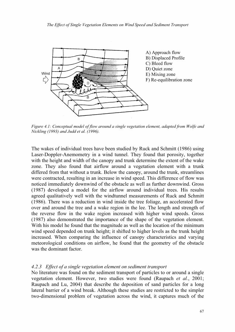
The Effect of Single Vegetation Elements on Wind Speed and Sediment Transport
67
Figure 4.1: Conceptual model of flow around a single vegetation element, adapted from Wolfe and Nickling (1993) and Judd et al. (1996).
The wakes of individual trees have been studied by Ruck and Schmitt (1986) using Laser-Doppler-Anemometry in a wind tunnel. They found that porosity, together with the height and width of the canopy and trunk determine the extent of the wake zone. They also found that airflow around a vegetation element with a trunk differed from that without a trunk. Below the canopy, around the trunk, streamlines were contracted, resulting in an increase in wind speed. This difference of flow was noticed immediately downwind of the obstacle as well as further downwind. Gross (1987) developed a model for the airflow around individual trees. His results agreed qualitatively well with the windtunnel measurements of Ruck and Schmitt (1986). There was a reduction in wind inside the tree foliage, an accelerated flow over and around the tree and a wake region in the lee. The length and strength of the reverse flow in the wake region increased with higher wind speeds. Gross (1987) also demonstrated the importance of the shape of the vegetation element. With his model he found that the magnitude as well as the location of the minimum wind speed depended on trunk height; it shifted to higher levels as the trunk height increased. When comparing the influence of canopy characteristics and varying meteorological conditions on airflow, he found that the geometry of the obstacle was the dominant factor. 4.2.3 Effect of a single vegetation element on sediment transport No literature was found on the sediment transport of particles to or around a single vegetation element. However, two studies were found (Raupach et al., 2001; Raupach and Lu, 2004) that describe the deposition of sand particles for a long lateral barrier of a wind break. Although these studies are restricted to the simpler two-dimensional problem of vegetation across the wind, it captures much of the
A) Approach flow B) Displaced Profile C) Bleed flow D) Quiet zone E) Mixing zone F) Re-equilibration zone
Chapter 4
68
physics in the full three-dimensional problem (Raupach and Lu, 2004). When oncoming particle-laden airflow approaches the vegetation element, some of the oncoming air passes over the obstacle, while some flows through it. In the air flowing over the obstacle, particle concentrations are not much different from the approach flow (Raupach et al., 2001). In the flow that passes through the obstacle, particles are filtered from the flow and deposited onto vegetation elements. The fraction of particles in the oncoming flow which pass through the windbreak is related to the optical porosity of the windbreak. In the lee of the windbreak, wind speed is reduced, causing a reduction in sediment transport. Thus, there is a deposition of particles to the obstacle, together with a reduction in deposition to the downwind surface. This reduction in sediment transport was caused by the reduced particle concentration and the reduced wind speed in the downwind sheltered region. With increasing downwind distance, particles from the flow above are mixed downwards into the sheltered region. This results in an increase in both near-surface particle concentration and surface deposition. Eventually the same concentration of particles is found as that far upwind of the obstacle (Raupach et al., 2001) . The shelter effect of porous wind fences on wind erosion of sand particles was studied experimentally by Lee et al. (2002), who found a fence with a porosity of 30 % the most effective in diminishing wind blown sand particles. It was furthermore noticed that areas of backward sediment transport were related to the recirculating flows that were formed behind the wind fence. With an increase in the porosity of the fence, the location of the backward sediment shifted further downwind. Whether this holds for single vegetation elements is presently unknown. 4.3 Materials and Methods 4.3.1 Study Site Field measurements were carried out in a farmers’ field ± 7 km east of Dori in north Burkina Faso. The area is part of the southern Sahelian zone, which is characterized by high temperatures all year round and a short rainy season of 4 months, from June to September. The average annual rainfall is 420 mm.
In the early rainy season in the Sahel, heavy thunderstorms develop that bring the first rains. In this period of the year severe wind erosion may occur, because the thunderstorms are often accompanied by strong winds that precede rainfall. These winds are the result of strong downdrafts within the thunderstorm cloud, which cause a forward outflow of cold air. Although the storms are usually of short duration (10 to 30 minutes), they may result in intense soil movement, especially on unprotected soils (Michels et al., 1995; Sterk et al., 1998).
The soil texture in the experimental field was loamy sand, with 85.5 % sand, 11.1 % silt and 3.4 % clay. The median particle size was 141 µm. The main crop in
The Effect of Single Vegetation Elements on Wind Speed and Sediment Transport
69
the field was pearl millet (Pennisetum glaucum), intercropped with cowpea (Vigna unguiculata). Within the field, natural vegetation was present. The density of vegetation elements larger than 0.5 m height was 70 elements per hectare. Most of these vegetation elements comprised shrubs (87 %). The most common tree and shrub species in the field were Piliostigma reticulatum, Faidherbia albida, Balanites aegyptiaca, Sclerocarya birrea and Ziziphus mauritiana. 4.3.2 Equipment Wind speed was measured with sonic anemometers. A sonic anemometer is a wind sensor, with no moving parts, that measures three dimensional wind velocity at a high frequency. The measurement technique is based on the transit times of ultrasonic acoustic signals. The principles of sonic anemometry are extensively described in several textbooks (e.g. Kaimal and Finnigan, 1994). In this study three sonic anemometers of Young Meteorological Instruments, model 81000, were used. The sensor of this sonic anemometer consists of three pairs of sensor heads at an angle with each other. Wind speed is measured in three directions: vertical (ws-component), horizontal from east to west (us-component) and horizontal from north to south (vs-component), where the subscript s indicates the sonic anemometer. The measuring range of wind speed was 0 to 40 m s-1, with an accuracy of wind speed measurement of 1 % in the range of 0 to 30 m s-1 and 3 % above 30 m s-1. The internal sampling rate of the sensors is 160 Hz, while the sampling frequency used in this study was 16 Hz. Two sonic anemometers were connected to a CR10 datalogger of Campbell Scientific Ltd. that was powered by two batteries of 12V. One sonic anemometer was connected to a CR10X datalogger of Campbell Scientific Ltd., which was also powered by two batteries of 12V.
Sediment transport was measured with Modified Wilson and Cooke (MWAC) catchers (Figure 4.2; for more details see Sterk and Raats, 1996). The catchers used in this study trap moving material across five heights. The intended measuring heights were 0.05, 0.12, 0.19, 0.26 and 0.75 meter above the soil surface. But these values could change 5 to 20 mm because of soil surface changes. Each trap consists of a plastic bottle with an inlet and an outlet glass tube, mounted horizontally on a mast that rotates about a central pole. A wind vane connected to the mast ensures that the inlet of the glass tube is pointed into the wind. The sediment that is transported in the air enters the inlet glass tube together with the air and settles in the sample bottle. The air escapes through the outlet glass tube. The inlet and the outlet of the glass tubes have an internal diameter of 8 mm, the opening of the glass tube is thus 50.3 mm2. In order to determine the duration of a wind storm prior to rainfall, a tipping bucket rain gauge was used to measure rainfall. Its registration time was set to one minute.
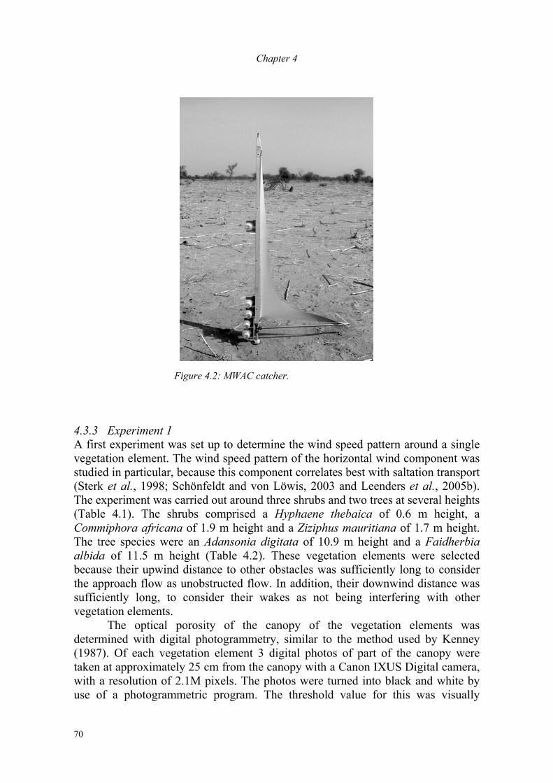
Chapter 4
70
Figure 4.2: MWAC catcher. 4.3.3 Experiment 1 A first experiment was set up to determine the wind speed pattern around a single vegetation element. The wind speed pattern of the horizontal wind component was studied in particular, because this component correlates best with saltation transport (Sterk et al., 1998; Schönfeldt and von Löwis, 2003 and Leenders et al., 2005b). The experiment was carried out around three shrubs and two trees at several heights (Table 4.1). The shrubs comprised a Hyphaene thebaica of 0.6 m height, a Commiphora africana of 1.9 m height and a Ziziphus mauritiana of 1.7 m height. The tree species were an Adansonia digitata of 10.9 m height and a Faidherbia albida of 11.5 m height (Table 4.2). These vegetation elements were selected because their upwind distance to other obstacles was sufficiently long to consider the approach flow as unobstructed flow. In addition, their downwind distance was sufficiently long, to consider their wakes as not being interfering with other vegetation elements.
The optical porosity of the canopy of the vegetation elements was determined with digital photogrammetry, similar to the method used by Kenney (1987). Of each vegetation element 3 digital photos of part of the canopy were taken at approximately 25 cm from the canopy with a Canon IXUS Digital camera, with a resolution of 2.1M pixels. The photos were turned into black and white by use of a photogrammetric program. The threshold value for this was visually
The Effect of Single Vegetation Elements on Wind Speed and Sediment Transport
71
determined. The percentage of white pixels in the photo was taken as the porosity of the canopy. This value of porosity is the optical porosity, which is not the same as the volumetric porosity. Generally the optical porosity is an underestimation of the volumetric porosity because much of the small scale porosity (between leaves and branches) is beyond the resolution of analysis and the vegetation elements obscures transmission of light through it (Grant and Nickling, 1998).
One of the sonic anemometers was used as a reference in the experiment. It was placed upwind of the experimental plot, in a non-distorted environment. The other two sensors were placed in a grid around the vegetation element in the direction of the wind in such a way that wind speed was measured on 19 locations in 11 runs (Figure 4.3). In order to provide sufficient data in front and behind of the vegetation element, the measuring period for the positions at the centreline was set to 30 minutes. On the other locations wind speed was measured for 15 minutes. The total sampling time was 225 minutes. For each run, the start and end time were noted, as well as the wind direction and distance from the vegetation element.
Table 4.1: Height of wind measurements and number of times Experiment 1 was carried out.
Species Height of measurement [m]
Number of experiment [-]
Shrub Hyphaene thebaica 0.40 2 Commiphora africana
0.45 0.65 0.85
2 2 1
Ziziphus mauritiana
0.40 0.60 0.80
2 1 1
Tree Adansonia digitata
1.25 1.50 2.5 3.8
1 2 2 2
Faidherbia albida
1.25 2.5 3.8
2 1 2
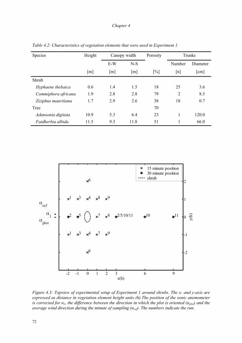
Chapter 4
72
Table 4.2: Characteristics of vegetation elements that were used in Experiment 1.
Species Height Canopy width Porosity Trunks
E-W N-S Number Diameter
[m] [m] [m] [%] [n] [cm]
Shrub Hyphaene thebaica 0.6 1.4 1.5 18 25 3.6 Commiphora africana 1.9 2.8 2.8 79 2 8.5 Ziziphus mauritiana 1.7 2.9 2.6 38 18 0.7 Tree 70 Adansonia digitata 10.9 5.3 6.4 23 1 120.0 Faidherbia albida 11.5 9.3 11.8 51 1 66.0
αplot
αref
α1
-2 -1 0 1 2 3 6 9
-2
-1
0
1
2
1
1
3
3
6
4
4
6
7
7
8
9
8
9
2 5 2/5/10/11 10 11
x(h)
y(h)
15 minute position30 minute positionshrub
Figure 4.3: Topview of experimental setup of Experiment 1 around shrubs. The x- and y-axis are expressed as distance in vegetation element height units (h).The position of the sonic anemometer is corrected for α1, the difference between the direction in which the plot is oriented (αplot) and the average wind direction during the minute of sampling (αref). The numbers indicate the run.
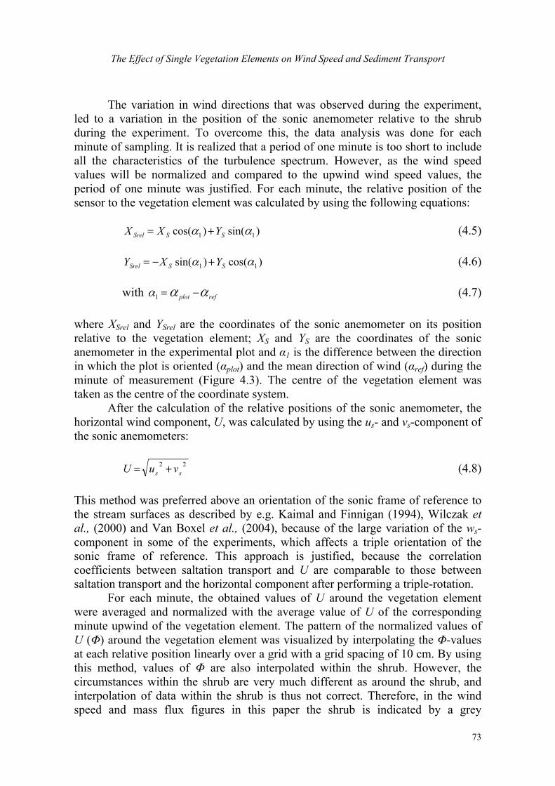
The Effect of Single Vegetation Elements on Wind Speed and Sediment Transport
73
The variation in wind directions that was observed during the experiment, led to a variation in the position of the sonic anemometer relative to the shrub during the experiment. To overcome this, the data analysis was done for each minute of sampling. It is realized that a period of one minute is too short to include all the characteristics of the turbulence spectrum. However, as the wind speed values will be normalized and compared to the upwind wind speed values, the period of one minute was justified. For each minute, the relative position of the sensor to the vegetation element was calculated by using the following equations:
)sin()cos( 11 αα SSSrel YXX += (4.5)
)cos()sin( 11 αα SSSrel YXY +−= (4.6)
with refplot ααα −=1 (4.7)
where XSrel and YSrel are the coordinates of the sonic anemometer on its position relative to the vegetation element; XS and YS are the coordinates of the sonic anemometer in the experimental plot and α1 is the difference between the direction in which the plot is oriented (αplot) and the mean direction of wind (αref) during the minute of measurement (Figure 4.3). The centre of the vegetation element was taken as the centre of the coordinate system. After the calculation of the relative positions of the sonic anemometer, the horizontal wind component, U, was calculated by using the us- and vs-component of the sonic anemometers:
22ss vuU += (4.8)
This method was preferred above an orientation of the sonic frame of reference to the stream surfaces as described by e.g. Kaimal and Finnigan (1994), Wilczak et al., (2000) and Van Boxel et al., (2004), because of the large variation of the ws-component in some of the experiments, which affects a triple orientation of the sonic frame of reference. This approach is justified, because the correlation coefficients between saltation transport and U are comparable to those between saltation transport and the horizontal component after performing a triple-rotation.
For each minute, the obtained values of U around the vegetation element were averaged and normalized with the average value of U of the corresponding minute upwind of the vegetation element. The pattern of the normalized values of U (Φ) around the vegetation element was visualized by interpolating the Φ-values at each relative position linearly over a grid with a grid spacing of 10 cm. By using this method, values of Φ are also interpolated within the shrub. However, the circumstances within the shrub are very much different as around the shrub, and interpolation of data within the shrub is thus not correct. Therefore, in the wind speed and mass flux figures in this paper the shrub is indicated by a grey
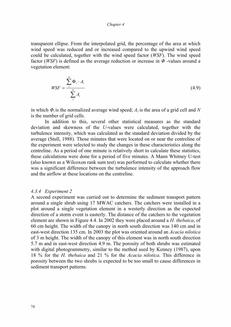
Chapter 4
74
transparent ellipse. From the interpolated grid, the percentage of the area at which wind speed was reduced and or increased compared to the upwind wind speed could be calculated, together with the wind speed factor (WSF). The wind speed factor (WSF) is defined as the average reduction or increase in Φ -values around a vegetation element:
∑
∑ ⋅Φ= N
ii
i
N
ii
A
AWSF (4.9)
in which Φi is the normalized average wind speed; Ai is the area of a grid cell and N is the number of grid cells.
In addition to this, several other statistical measures as the standard deviation and skewness of the U-values were calculated, together with the turbulence intensity, which was calculated as the standard deviation divided by the average (Stull, 1988). Those minutes that were located on or near the centreline of the experiment were selected to study the changes in these characteristics along the centreline. As a period of one minute is relatively short to calculate these statistics, these calculations were done for a period of five minutes. A Mann Whitney U-test (also known as a Wilcoxon rank sum test) was performed to calculate whether there was a significant difference between the turbulence intensity of the approach flow and the airflow at these locations on the centreline. 4.3.4 Experiment 2 A second experiment was carried out to determine the sediment transport pattern around a single shrub using 17 MWAC catchers. The catchers were installed in a plot around a single vegetation element in a westerly direction as the expected direction of a storm event is easterly. The distance of the catchers to the vegetation element are shown in Figure 4.4. In 2002 they were placed around a H. thebaica, of 60 cm height. The width of the canopy in north south direction was 140 cm and in east-west direction 135 cm. In 2003 the plot was oriented around an Acacia nilotica of 3 m height. The width of the canopy of this element was in north south direction 5.7 m and in east-west direction 4.9 m. The porosity of both shrubs was estimated with digital photogrammetry, similar to the method used by Kenney (1987), upon 18 % for the H. thebaica and 21 % for the Acacia nilotica. This difference in porosity between the two shrubs is expected to be too small to cause differences in sediment transport patterns.
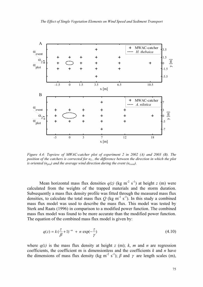
The Effect of Single Vegetation Elements on Wind Speed and Sediment Transport
75
-1.5 0 1.5 3.5 6.5 10.5
-3.5
-1.5
0
1.5
3.5
x [m]
y [m
]
MWAC-catcher H. thebaica
-3 0 3 7 12 18
-7
-3
0
3
7
x [m]
y [m
]
MWAC-catcher A. nilotica
A
B
αplot
αevent
α2
αplot
αevent
α2
Figure 4.4: Topview of MWAC-catcher plot of experiment 2 in 2002 (A) and 2003 (B). The position of the catchers is corrected for α2 , the difference between the direction in which the plot is oriented (αplot) and the average wind direction during the event (αevent).
Mean horizontal mass flux densities q(z) (kg m-2 s-1) at height z (m) were
calculated from the weights of the trapped materials and the storm duration. Subsequently a mass flux density profile was fitted through the measured mass flux densities, to calculate the total mass flux Q (kg m-1 s-1). In this study a combined mass flux model was used to describe the mass flux. This model was tested by Sterk and Raats (1996) in comparison to a modified power function. The combined mass flux model was found to be more accurate than the modified power function. The equation of the combined mass flux model is given by:
)exp()1()(γβznzkzq m −++= − (4.10)
where q(z) is the mass flux density at height z (m); k, m and n are regression coefficients, the coefficient m is dimensionless and the coefficients k and n have the dimensions of mass flux density (kg m-2 s-1); β and γ are length scales (m),
Chapter 4
76
taken as 1 m in this study. An extensive description of the model and the fitting method can be found in Sterk and Raats (1996).
The fitted mass flux density profile was integrated over height from 0 to 1 m, to calculate the mass flux at the sampling location (kg m-1 s-1) up to 1 m above the soil surface. The total mass flux, Qt (kg m-1 s-1), was obtained by dividing Q by the trapping efficiency of the catcher. According to Sterk (1993) the overall trapping efficiency of the MWAC catcher is 0.49 with a standard deviation of 0.03. This was based on 12 runs in a wind tunnel with wind speeds ranging from 9.9 to 11.5 m s-1. Goossens et al. (2000) found an overall efficiency twice as high, based on 15 runs in a wind tunnel with wind speeds ranging from 6.6 to 14.4 m s-1. These differences in efficiencies are crucial in studies on the quantification of sediment transport. However, the results of this study are not affected because the sediment transport values are studied relative to each other for the pattern of sediment transport.
After the calculation of the total mass flux measured by each MWAC catcher around the shrub, the relative position of the MWAC catcher to the shrub was calculated for each storm, by using equations similar to equation 4.5 to 4.7:
)sin()cos( 22 αα MMMrel YXX += (4.11)
)cos()sin( 22 αα MMMrel YXY +−= (4.12)
with eventplot ααα −=2 (4.13)
where XMrel and YMrel are the coordinates of the MWAC catcher on its position relative to the vegetation element; XM and YM are the coordinates of the MWAC catcher in the experimental plot and 2α is the difference between the direction in which the plot is oriented ( plotα ), which is westerly, thus 270 degrees, and the mean direction of wind ( eventα ) during the storm. The centre of the shrub is taken as (0,0)-coordinate. For both shrubs, a zone was defined in which the sediment transport was thought to be affected by the shrub. The borders of this ‘influence zone’ were for the H. thebaica set to -2 and 12 m in the east-west direction and -2 and +2 m in the north-south direction. For the Acacia nilotica they were set to -6 m and +30 m in the east-west direction and -5 and +5 m in the north-south direction.
The fluxes measured by the catchers that had a relative position within this zone were normalized using the average mass flux of those catchers that had a relative position outside this zone as the reference. The result was a normalized sediment transport factor (ψ). Because of this and the correction for wind direction for each event, the total mass flux values of several events could be projected within one picture. The pattern of total mass flux values around each shrub was visualized by interpolating the normalized mass fluxes at each relative position over a grid with a grid spacing of 10 cm. As the data within the area of the shrub are uncertain, because the typical circumstances within a shrub differ from those
The Effect of Single Vegetation Elements on Wind Speed and Sediment Transport
77
around, the shrub was indicated by an ellipse. Based on the interpolated grid, the percentage of the area was calculated at which total mass flux was reduced or increased compared to the average value of total mass flux of the reference catchers (ψ). This was done for each event. A sediment factor, defined as the average reduction or increase in total mass flux was also calculated. These parameters were combined to calculate the net effect on sediment transport (STF) around the vegetation element:
∑
∑ ⋅= N
ii
i
N
ii
A
ASTF
ψ (4.14)
in which ψi is the normalized total mass flux; Ai is the area of a grid cell and N is the number of grid cells. 4.4 Results and Discussion 4.4.1 Wind speed around a single vegetation element The measurements of wind speed patterns around single vegetation elements were carried out around five vegetation elements (Table 4.1). Here the results for two shrubs, the H. thebaica and the C. africana, and one tree, the F. albida will be discussed. The results of the measurements around the Z. mauritiana and the A. digitata were similar to those discussed. The measurements were carried out on windy days. Approach wind speeds, as measured upwind from the vegetation element, varied typically between 2.5 and 3.9 m s-1 (one minute averages) at the measuring height (Table 4.3). The range in wind directions during the experiment varied from 45 degrees for the C. africana at 0.45 m height to 127 degrees for the H. thebaica at 0.4 m height (Table 4.3). The maximum number of minutes of wind speed measurements that were discarded from further analysis, as a consequence of the variation in wind direction was 51 for the F. albida at 3.8 m height. This was 11.3 % of the measurements. This means that for each dataset at least 399 data points were used for the interpolation of wind speed around a vegetation element. The figures that were obtained from interpolation of wind speed measurements (Figures 4.5, 4.7 and 4.8) were analyzed regarding the general pattern that is visible in these figures. The scatter, which is present as well, was not analyzed in detail. The scatter was partly ascribed to the morphology within a vegetation element (e.g. gaps in the canopy) and to the short averaging time of one minute.
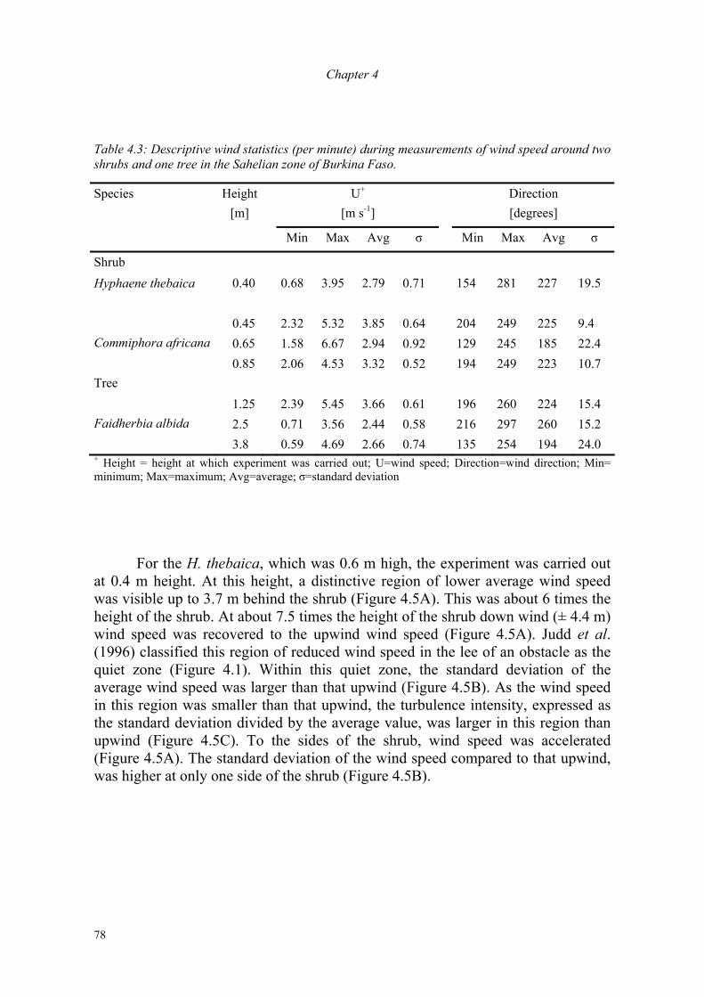
Chapter 4
78
Table 4.3: Descriptive wind statistics (per minute) during measurements of wind speed around two shrubs and one tree in the Sahelian zone of Burkina Faso.
Species Height [m]
U+
[m s-1] Direction
[degrees]
Min Max Avg σ Min Max Avg σ
Shrub Hyphaene thebaica 0.40 0.68 3.95 2.79 0.71 154 281 227 19.5 0.45 2.32 5.32 3.85 0.64 204 249 225 9.4 Commiphora africana 0.65 1.58 6.67 2.94 0.92 129 245 185 22.4 0.85 2.06 4.53 3.32 0.52 194 249 223 10.7 Tree 1.25 2.39 5.45 3.66 0.61 196 260 224 15.4 Faidherbia albida 2.5 0.71 3.56 2.44 0.58 216 297 260 15.2 3.8 0.59 4.69 2.66 0.74 135 254 194 24.0 + Height = height at which experiment was carried out; U=wind speed; Direction=wind direction; Min= minimum; Max=maximum; Avg=average; σ=standard deviation
For the H. thebaica, which was 0.6 m high, the experiment was carried out
at 0.4 m height. At this height, a distinctive region of lower average wind speed was visible up to 3.7 m behind the shrub (Figure 4.5A). This was about 6 times the height of the shrub. At about 7.5 times the height of the shrub down wind (± 4.4 m) wind speed was recovered to the upwind wind speed (Figure 4.5A). Judd et al. (1996) classified this region of reduced wind speed in the lee of an obstacle as the quiet zone (Figure 4.1). Within this quiet zone, the standard deviation of the average wind speed was larger than that upwind (Figure 4.5B). As the wind speed in this region was smaller than that upwind, the turbulence intensity, expressed as the standard deviation divided by the average value, was larger in this region than upwind (Figure 4.5C). To the sides of the shrub, wind speed was accelerated (Figure 4.5A). The standard deviation of the wind speed compared to that upwind, was higher at only one side of the shrub (Figure 4.5B).
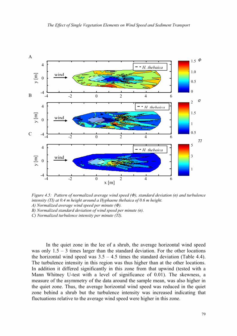
The Effect of Single Vegetation Elements on Wind Speed and Sediment Transport
79
Figure 4.5: Pattern of normalized average wind speed (Φ), standard deviation (σ) and turbulence intensity (TI) at 0.4 m height around a Hyphaene thebaica of 0.6 m height. A) Normalized average wind speed per minute (Φ). B) Normalized standard deviation of wind speed per minute (σ). C) Normalized turbulence intensity per minute (TI).
In the quiet zone in the lee of a shrub, the average horizontal wind speed
was only 1.5 – 3 times larger than the standard deviation. For the other locations the horizontal wind speed was 3.5 – 4.5 times the standard deviation (Table 4.4). The turbulence intensity in this region was thus higher than at the other locations. In addition it differed significantly in this zone from that upwind (tested with a Mann Whitney U-test with a level of significance of 0.01). The skewness, a measure of the asymmetry of the data around the sample mean, was also higher in the quiet zone. Thus, the average horizontal wind speed was reduced in the quiet zone behind a shrub but the turbulence intensity was increased indicating that fluctuations relative to the average wind speed were higher in this zone.
1.5
0
0.5
1.0
2
0.5
1
1.5
H. thebaica
wind
4
-4
0
y [m
]
-4 -2 0 6 2 4
H. thebaica
wind
4
-4
0 y [m
]
-4 -2 0 6 2 4
H. thebaica
wind
4
-4
0
y [m
]
-4 -2 0 6 2 4
5
1
3
Φ σ TI
A B C
x [m]
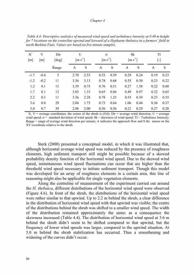
Chapter 4
80
Table 4.4: Descriptive statistics of measured wind speed and turbulence intensity at 0.40 m height for 7 locations on the centreline upwind and leeward of a Hyphaene thebaica in a farmers’ field in north Burkina Faso. Values are based on five minute samples.
X+
[m] Y
[m]
Dir [deg]
U
[m s-1]
σ [m s-1]
Sk
[m s-1]
TI [-]
Range A S A S A S A S
-1.7 -0.4 5 2.70 2.53 0.53 0.59 0.29 0.24 0.19 0.23-1.2 -0.2 11 3.36 3.13 0.78 0.68 0.55 0.30 0.23 0.221.2 0.1 13 3.39 0.75 0.76 0.51 0.27 1.58 0.22 0.681.7 0.1 12 3.03 1.33 0.65 0.86 0.49 0.97 0.22 0.652.2 0.3 11 3.36 2.28 0.78 1.25 0.55 0.39 0.23 0.553.6 0.0 29 2.04 1.73 0.73 0.64 1.06 0.44 0.36 0.375.0 0.7 39 2.06 2.00 0.56 0.56 0.21 0.29 0.27 0.28
+ X, Y = average coordinates, the centre of the shrub is (0,0); Dir = average wind direction; U = average wind speed; σ = standard deviation of wind speed; Sk = skewness of wind speed; TI = Turbulence Intensity; Range = range of average wind direction per minute; A indicates the approach flow and S the sensor on the XY coordinate relative to the shrub.
Sterk (2000) presented a conceptual model, in which it was illustrated that,
although horizontal average wind speed was reduced by the presence of roughness elements, high sediment transport still might be possible because of a skewed probability density function of the horizontal wind speed. Due to the skewed wind speed, instantaneous wind speed fluctuations can occur that are higher than the threshold wind speed necessary to initiate sediment transport. Though this model was developed for an array of roughness elements in a certain area, this line of reasoning might also be applicable for single vegetation elements.
Along the centreline of measurement of the experiment carried out around the H. thebaica, different distributions of the horizontal wind speed were observed (Figure 4.6). In front of the shrub, the distributions of the horizontal wind speed were rather similar to that upwind. Up to 2.2 m behind the shrub, a clear difference in the distribution of horizontal wind speed with that upwind was visible; the centre of the distributions behind the shrub was shifted to a smaller wind speed. The width of the distribution remained approximately the same; as a consequence the skewness increased (Table 4.4). The distribution of horizontal wind speed at 3.6 m behind the shrub didn’t seem to be shifted compared to that upwind, but the frequency of lower wind speeds was larger, compared to the upwind situation. At 5.0 m behind the shrub stabilization has occurred. Thus a smoothening and widening of the curves didn’t occur.
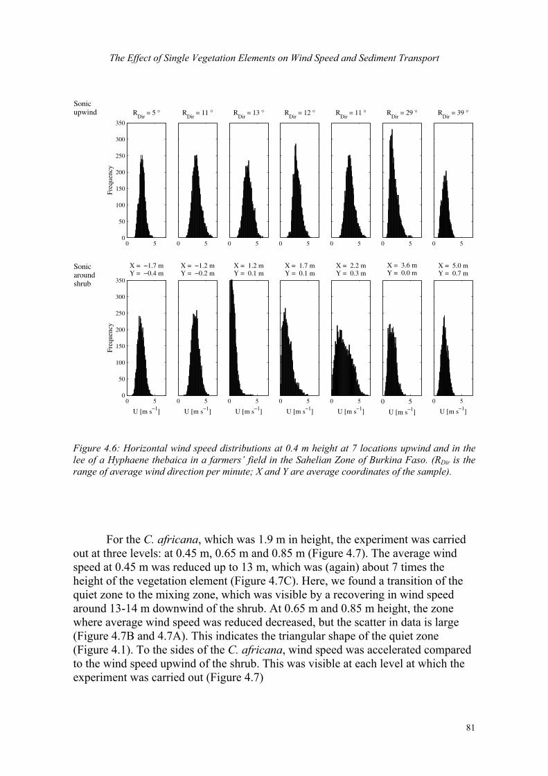
The Effect of Single Vegetation Elements on Wind Speed and Sediment Transport
81
0 50
50
100
150
200
250
300
350
Freq
uenc
yR
Dir = 5 °
0 5
RDir
= 11 °
0 5
RDir
= 13 °
0 5
RDir
= 12 °
0 5
RDir
= 11 °
0 5
RDir
= 29 °
0 5
RDir
= 39 °
0 50
50
100
150
200
250
300
350
Freq
uenc
y
U [m s−1]
X = −1.7 mY = −0.4 m
0 5
U [m s−1]
X = −1.2 mY = −0.2 m
0 5
U [m s−1]
X = 1.2 mY = 0.1 m
0 5
U [m s−1]
X = 1.7 mY = 0.1 m
0 5
U [m s−1]
X = 2.2 mY = 0.3 m
0 5
U [m s−1]
X = 3.6 mY = 0.0 m
0 5
U [m s−1]
X = 5.0 mY = 0.7 m
Sonicupwind
Sonicaroundshrub
Figure 4.6: Horizontal wind speed distributions at 0.4 m height at 7 locations upwind and in the lee of a Hyphaene thebaica in a farmers’ field in the Sahelian Zone of Burkina Faso. (RDir is the range of average wind direction per minute; X and Y are average coordinates of the sample). For the C. africana, which was 1.9 m in height, the experiment was carried out at three levels: at 0.45 m, 0.65 m and 0.85 m (Figure 4.7). The average wind speed at 0.45 m was reduced up to 13 m, which was (again) about 7 times the height of the vegetation element (Figure 4.7C). Here, we found a transition of the quiet zone to the mixing zone, which was visible by a recovering in wind speed around 13-14 m downwind of the shrub. At 0.65 m and 0.85 m height, the zone where average wind speed was reduced decreased, but the scatter in data is large (Figure 4.7B and 4.7A). This indicates the triangular shape of the quiet zone (Figure 4.1). To the sides of the C. africana, wind speed was accelerated compared to the wind speed upwind of the shrub. This was visible at each level at which the experiment was carried out (Figure 4.7)
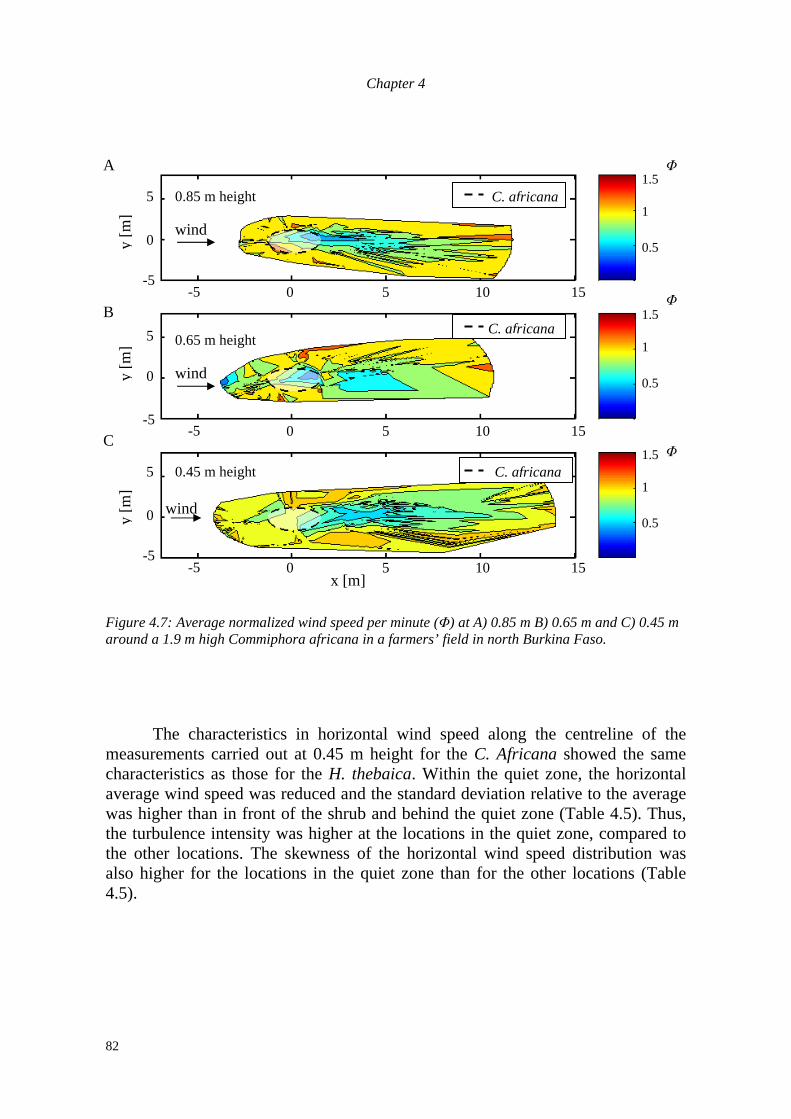
Chapter 4
82
Figure 4.7: Average normalized wind speed per minute (Φ) at A) 0.85 m B) 0.65 m and C) 0.45 m around a 1.9 m high Commiphora africana in a farmers’ field in north Burkina Faso.
The characteristics in horizontal wind speed along the centreline of the
measurements carried out at 0.45 m height for the C. Africana showed the same characteristics as those for the H. thebaica. Within the quiet zone, the horizontal average wind speed was reduced and the standard deviation relative to the average was higher than in front of the shrub and behind the quiet zone (Table 4.5). Thus, the turbulence intensity was higher at the locations in the quiet zone, compared to the other locations. The skewness of the horizontal wind speed distribution was also higher for the locations in the quiet zone than for the other locations (Table 4.5).
C. africana
C. africana
C. africana
wind
0.85 m height
wind
0.65 m height
wind
0.45 m height
-5 5 10 0 15
-5 5 10 0 15
-5 5 10 0 15
-5
5
0 y [m
]
-5
5
0 y [m
]
-5
5
0 y [m
]
x [m]
1.5
1
0.5
1.5
1
0.5
1.5
1
0.5
Φ Φ Φ
A B C
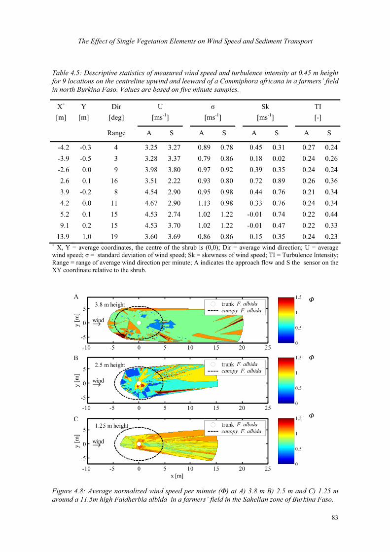
The Effect of Single Vegetation Elements on Wind Speed and Sediment Transport
83
Table 4.5: Descriptive statistics of measured wind speed and turbulence intensity at 0.45 m height for 9 locations on the centreline upwind and leeward of a Commiphora africana in a farmers’ field in north Burkina Faso. Values are based on five minute samples.
X+
[m] Y
[m] Dir
[deg] U
[ms-1] σ
[ms-1] Sk
[ms-1] TI
[-]
Range A S A S A S A S
-4.2 -0.3 4 3.25 3.27 0.89 0.78 0.45 0.31 0.27 0.24-3.9 -0.5 3 3.28 3.37 0.79 0.86 0.18 0.02 0.24 0.26-2.6 0.0 9 3.98 3.80 0.97 0.92 0.39 0.35 0.24 0.242.6 0.1 16 3.51 2.22 0.93 0.80 0.72 0.89 0.26 0.363.9 -0.2 8 4.54 2.90 0.95 0.98 0.44 0.76 0.21 0.344.2 0.0 11 4.67 2.90 1.13 0.98 0.33 0.76 0.24 0.345.2 0.1 15 4.53 2.74 1.02 1.22 -0.01 0.74 0.22 0.449.1 0.2 15 4.53 3.70 1.02 1.22 -0.01 0.47 0.22 0.33
13.9 1.0 19 3.60 3.69 0.86 0.86 0.15 0.35 0.24 0.23+ X, Y = average coordinates, the centre of the shrub is (0,0); Dir = average wind direction; U = average wind speed; σ = standard deviation of wind speed; Sk = skewness of wind speed; TI = Turbulence Intensity; Range = range of average wind direction per minute; A indicates the approach flow and S the sensor on the XY coordinate relative to the shrub.
-10 -5 0 5 10 15 20 25
-5
0
5
→wind
3.8 m height
y [m
]
trunk F. albidacanopy F. albida
0
0.5
1
1.5
-10 -5 0 5 10 15 20 25
-5
0
5
→wind
2.5 m height
y [m
]
trunk F. albidacanopy F. albida
0
0.5
1
1.5
-10 -5 0 5 10 15 20 25
-5
0
5
→wind
1.25 m height
x [m]
y [m
]
trunk F. albidacanopy F. albida
0
0.5
1
1.5
A
B
C
Figure 4.8: Average normalized wind speed per minute (Φ) at A) 3.8 m B) 2.5 m and C) 1.25 m around a 11.5m high Faidherbia albida in a farmers’ field in the Sahelian zone of Burkina Faso.
Φ Φ Φ
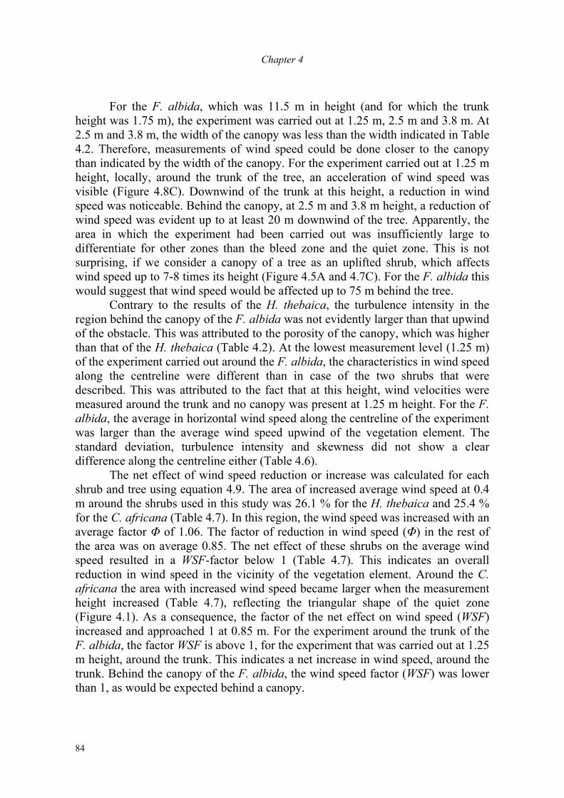
Chapter 4
84
For the F. albida, which was 11.5 m in height (and for which the trunk height was 1.75 m), the experiment was carried out at 1.25 m, 2.5 m and 3.8 m. At 2.5 m and 3.8 m, the width of the canopy was less than the width indicated in Table 4.2. Therefore, measurements of wind speed could be done closer to the canopy than indicated by the width of the canopy. For the experiment carried out at 1.25 m height, locally, around the trunk of the tree, an acceleration of wind speed was visible (Figure 4.8C). Downwind of the trunk at this height, a reduction in wind speed was noticeable. Behind the canopy, at 2.5 m and 3.8 m height, a reduction of wind speed was evident up to at least 20 m downwind of the tree. Apparently, the area in which the experiment had been carried out was insufficiently large to differentiate for other zones than the bleed zone and the quiet zone. This is not surprising, if we consider a canopy of a tree as an uplifted shrub, which affects wind speed up to 7-8 times its height (Figure 4.5A and 4.7C). For the F. albida this would suggest that wind speed would be affected up to 75 m behind the tree.
Contrary to the results of the H. thebaica, the turbulence intensity in the region behind the canopy of the F. albida was not evidently larger than that upwind of the obstacle. This was attributed to the porosity of the canopy, which was higher than that of the H. thebaica (Table 4.2). At the lowest measurement level (1.25 m) of the experiment carried out around the F. albida, the characteristics in wind speed along the centreline were different than in case of the two shrubs that were described. This was attributed to the fact that at this height, wind velocities were measured around the trunk and no canopy was present at 1.25 m height. For the F. albida, the average in horizontal wind speed along the centreline of the experiment was larger than the average wind speed upwind of the vegetation element. The standard deviation, turbulence intensity and skewness did not show a clear difference along the centreline either (Table 4.6).
The net effect of wind speed reduction or increase was calculated for each shrub and tree using equation 4.9. The area of increased average wind speed at 0.4 m around the shrubs used in this study was 26.1 % for the H. thebaica and 25.4 % for the C. africana (Table 4.7). In this region, the wind speed was increased with an average factor Φ of 1.06. The factor of reduction in wind speed (Φ) in the rest of the area was on average 0.85. The net effect of these shrubs on the average wind speed resulted in a WSF-factor below 1 (Table 4.7). This indicates an overall reduction in wind speed in the vicinity of the vegetation element. Around the C. africana the area with increased wind speed became larger when the measurement height increased (Table 4.7), reflecting the triangular shape of the quiet zone (Figure 4.1). As a consequence, the factor of the net effect on wind speed (WSF) increased and approached 1 at 0.85 m. For the experiment around the trunk of the F. albida, the factor WSF is above 1, for the experiment that was carried out at 1.25 m height, around the trunk. This indicates a net increase in wind speed, around the trunk. Behind the canopy of the F. albida, the wind speed factor (WSF) was lower than 1, as would be expected behind a canopy.
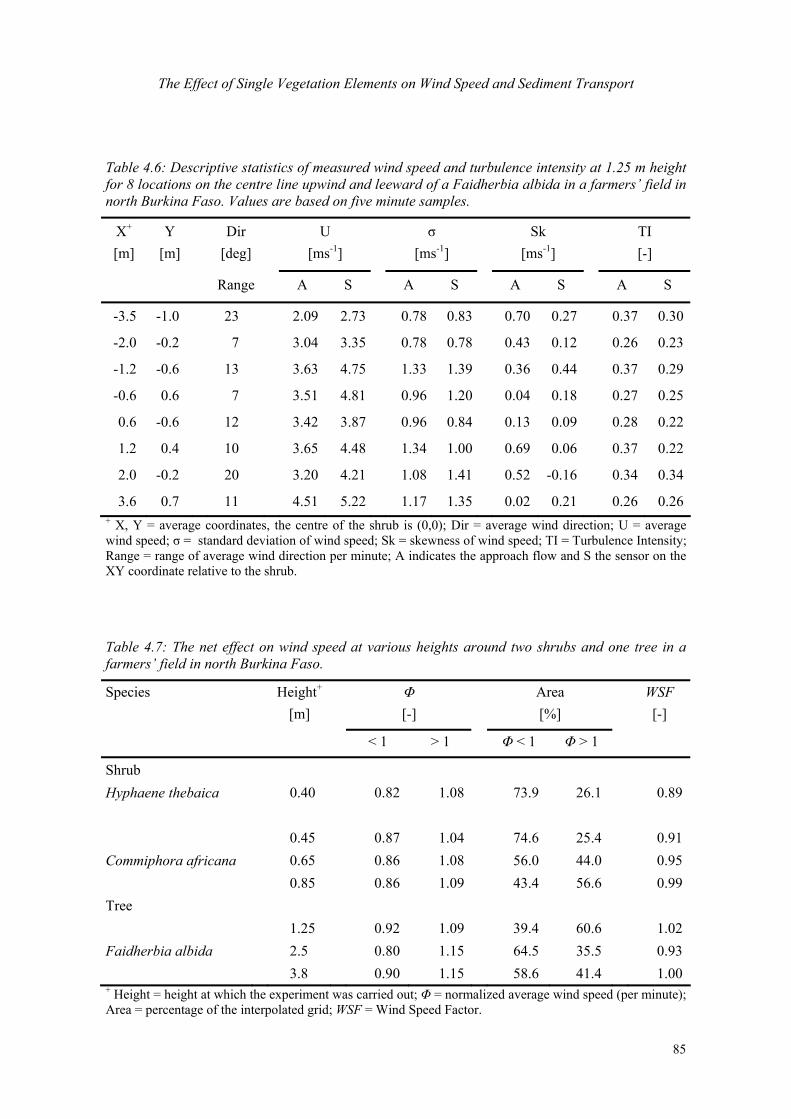
The Effect of Single Vegetation Elements on Wind Speed and Sediment Transport
85
Table 4.6: Descriptive statistics of measured wind speed and turbulence intensity at 1.25 m height for 8 locations on the centre line upwind and leeward of a Faidherbia albida in a farmers’ field in north Burkina Faso. Values are based on five minute samples.
X+
[m] Y
[m] Dir
[deg] U
[ms-1] σ
[ms-1] Sk
[ms-1] TI
[-]
Range A S A S A S A S
-3.5 -1.0 23 2.09 2.73 0.78 0.83 0.70 0.27 0.37 0.30
-2.0 -0.2 7 3.04 3.35 0.78 0.78 0.43 0.12 0.26 0.23
-1.2 -0.6 13 3.63 4.75 1.33 1.39 0.36 0.44 0.37 0.29
-0.6 0.6 7 3.51 4.81 0.96 1.20 0.04 0.18 0.27 0.25
0.6 -0.6 12 3.42 3.87 0.96 0.84 0.13 0.09 0.28 0.22
1.2 0.4 10 3.65 4.48 1.34 1.00 0.69 0.06 0.37 0.22
2.0 -0.2 20 3.20 4.21 1.08 1.41 0.52 -0.16 0.34 0.34
3.6 0.7 11 4.51 5.22 1.17 1.35 0.02 0.21 0.26 0.26+ X, Y = average coordinates, the centre of the shrub is (0,0); Dir = average wind direction; U = average wind speed; σ = standard deviation of wind speed; Sk = skewness of wind speed; TI = Turbulence Intensity; Range = range of average wind direction per minute; A indicates the approach flow and S the sensor on the XY coordinate relative to the shrub.
Table 4.7: The net effect on wind speed at various heights around two shrubs and one tree in a farmers’ field in north Burkina Faso.
Species
Height+
[m]
Φ [-]
Area [%]
WSF [-]
< 1 > 1 Φ < 1 Φ > 1
Shrub Hyphaene thebaica 0.40 0.82 1.08 73.9 26.1 0.89 0.45 0.87 1.04 74.6 25.4 0.91 Commiphora africana 0.65 0.86 1.08 56.0 44.0 0.95 0.85 0.86 1.09 43.4 56.6 0.99 Tree 1.25 0.92 1.09 39.4 60.6 1.02 Faidherbia albida 2.5 0.80 1.15 64.5 35.5 0.93 3.8 0.90 1.15 58.6 41.4 1.00 + Height = height at which the experiment was carried out; Φ = normalized average wind speed (per minute); Area = percentage of the interpolated grid; WSF = Wind Speed Factor.
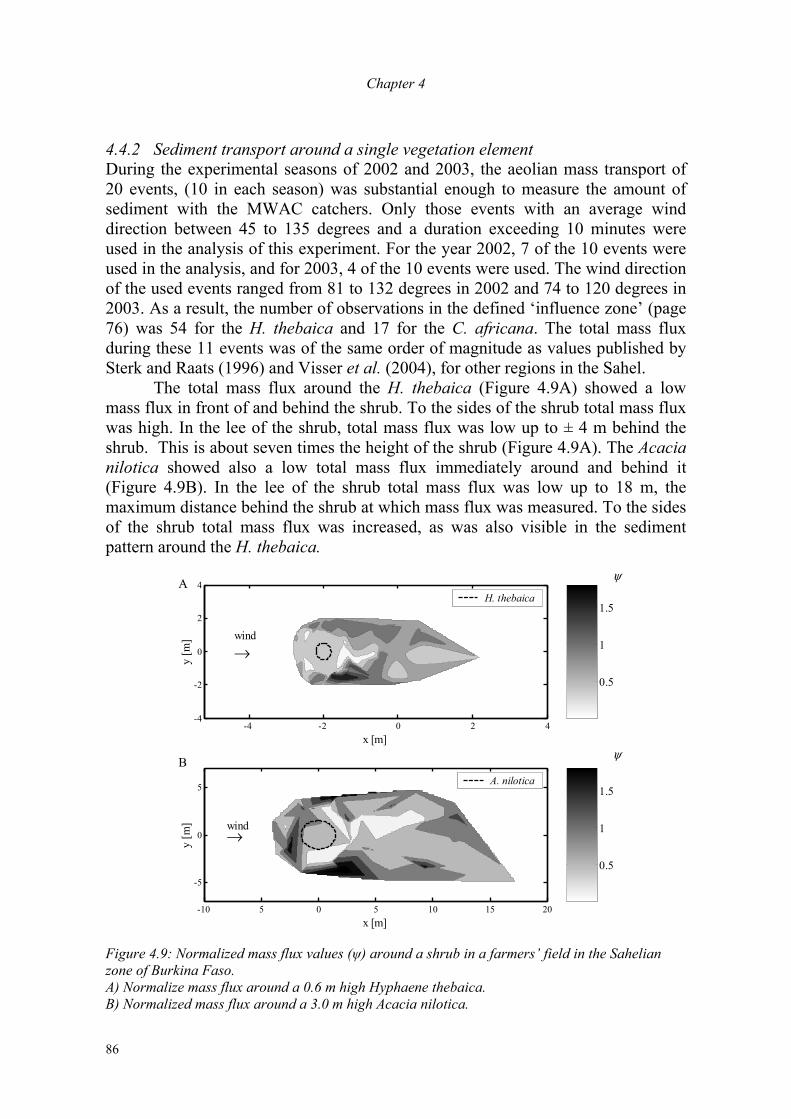
Chapter 4
86
4.4.2 Sediment transport around a single vegetation element During the experimental seasons of 2002 and 2003, the aeolian mass transport of 20 events, (10 in each season) was substantial enough to measure the amount of sediment with the MWAC catchers. Only those events with an average wind direction between 45 to 135 degrees and a duration exceeding 10 minutes were used in the analysis of this experiment. For the year 2002, 7 of the 10 events were used in the analysis, and for 2003, 4 of the 10 events were used. The wind direction of the used events ranged from 81 to 132 degrees in 2002 and 74 to 120 degrees in 2003. As a result, the number of observations in the defined ‘influence zone’ (page 76) was 54 for the H. thebaica and 17 for the C. africana. The total mass flux during these 11 events was of the same order of magnitude as values published by Sterk and Raats (1996) and Visser et al. (2004), for other regions in the Sahel. The total mass flux around the H. thebaica (Figure 4.9A) showed a low mass flux in front of and behind the shrub. To the sides of the shrub total mass flux was high. In the lee of the shrub, total mass flux was low up to ± 4 m behind the shrub. This is about seven times the height of the shrub (Figure 4.9A). The Acacia nilotica showed also a low total mass flux immediately around and behind it (Figure 4.9B). In the lee of the shrub total mass flux was low up to 18 m, the maximum distance behind the shrub at which mass flux was measured. To the sides of the shrub total mass flux was increased, as was also visible in the sediment pattern around the H. thebaica.
-4 -2 0 2 4-4
-2
0
2
4
→wind
x [m]
y [m
]
H. thebaica
0.5
1
1.5
-10 5 0 5 10 15 20
-5
0
5
→wind
x [m]
y [m
]
A. nilotica
0.5
1
1.5
A
B
ψ
ψ
Figure 4.9: Normalized mass flux values (ψ) around a shrub in a farmers’ field in the Sahelian zone of Burkina Faso. A) Normalize mass flux around a 0.6 m high Hyphaene thebaica. B) Normalized mass flux around a 3.0 m high Acacia nilotica.
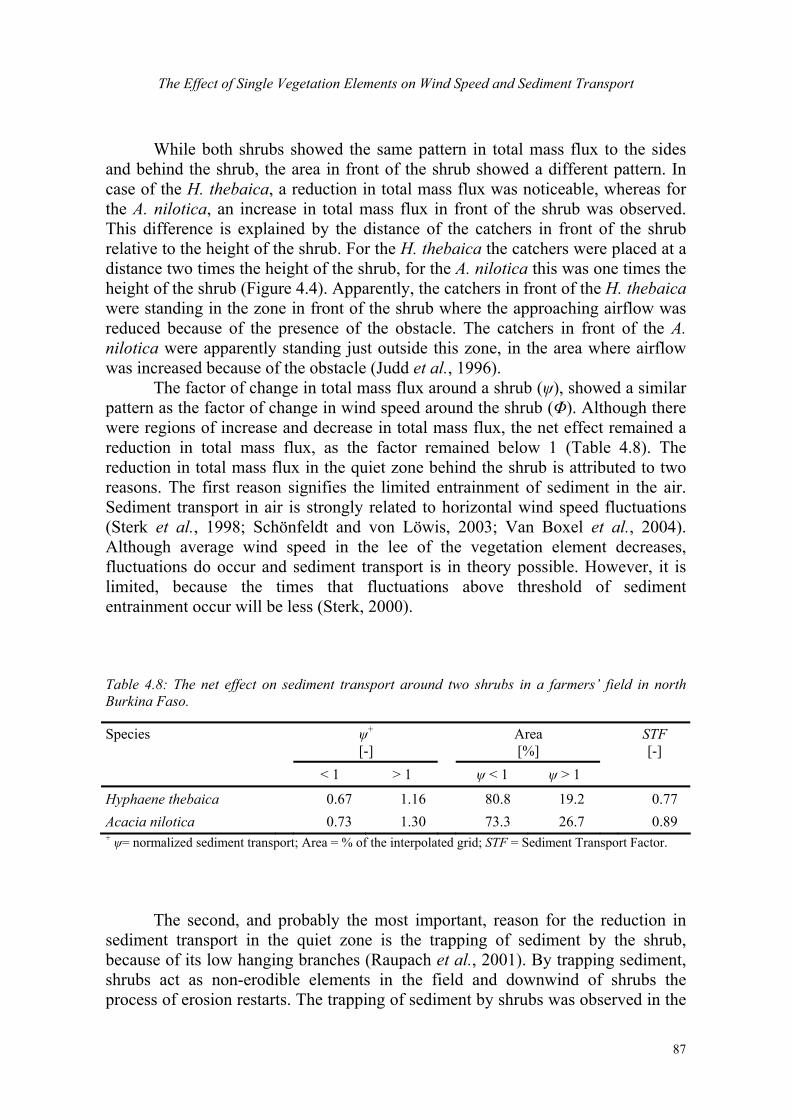
The Effect of Single Vegetation Elements on Wind Speed and Sediment Transport
87
While both shrubs showed the same pattern in total mass flux to the sides and behind the shrub, the area in front of the shrub showed a different pattern. In case of the H. thebaica, a reduction in total mass flux was noticeable, whereas for the A. nilotica, an increase in total mass flux in front of the shrub was observed. This difference is explained by the distance of the catchers in front of the shrub relative to the height of the shrub. For the H. thebaica the catchers were placed at a distance two times the height of the shrub, for the A. nilotica this was one times the height of the shrub (Figure 4.4). Apparently, the catchers in front of the H. thebaica were standing in the zone in front of the shrub where the approaching airflow was reduced because of the presence of the obstacle. The catchers in front of the A. nilotica were apparently standing just outside this zone, in the area where airflow was increased because of the obstacle (Judd et al., 1996).
The factor of change in total mass flux around a shrub (ψ), showed a similar pattern as the factor of change in wind speed around the shrub (Φ). Although there were regions of increase and decrease in total mass flux, the net effect remained a reduction in total mass flux, as the factor remained below 1 (Table 4.8). The reduction in total mass flux in the quiet zone behind the shrub is attributed to two reasons. The first reason signifies the limited entrainment of sediment in the air. Sediment transport in air is strongly related to horizontal wind speed fluctuations (Sterk et al., 1998; Schönfeldt and von Löwis, 2003; Van Boxel et al., 2004). Although average wind speed in the lee of the vegetation element decreases, fluctuations do occur and sediment transport is in theory possible. However, it is limited, because the times that fluctuations above threshold of sediment entrainment occur will be less (Sterk, 2000).
Table 4.8: The net effect on sediment transport around two shrubs in a farmers’ field in north Burkina Faso.
Species ψ+
[-] Area [%] STF
[-] < 1 > 1 ψ < 1 ψ > 1
Hyphaene thebaica 0.67 1.16 80.8 19.2 0.77 Acacia nilotica 0.73 1.30 73.3 26.7 0.89 + ψ= normalized sediment transport; Area = % of the interpolated grid; STF = Sediment Transport Factor.
The second, and probably the most important, reason for the reduction in
sediment transport in the quiet zone is the trapping of sediment by the shrub, because of its low hanging branches (Raupach et al., 2001). By trapping sediment, shrubs act as non-erodible elements in the field and downwind of shrubs the process of erosion restarts. The trapping of sediment by shrubs was observed in the
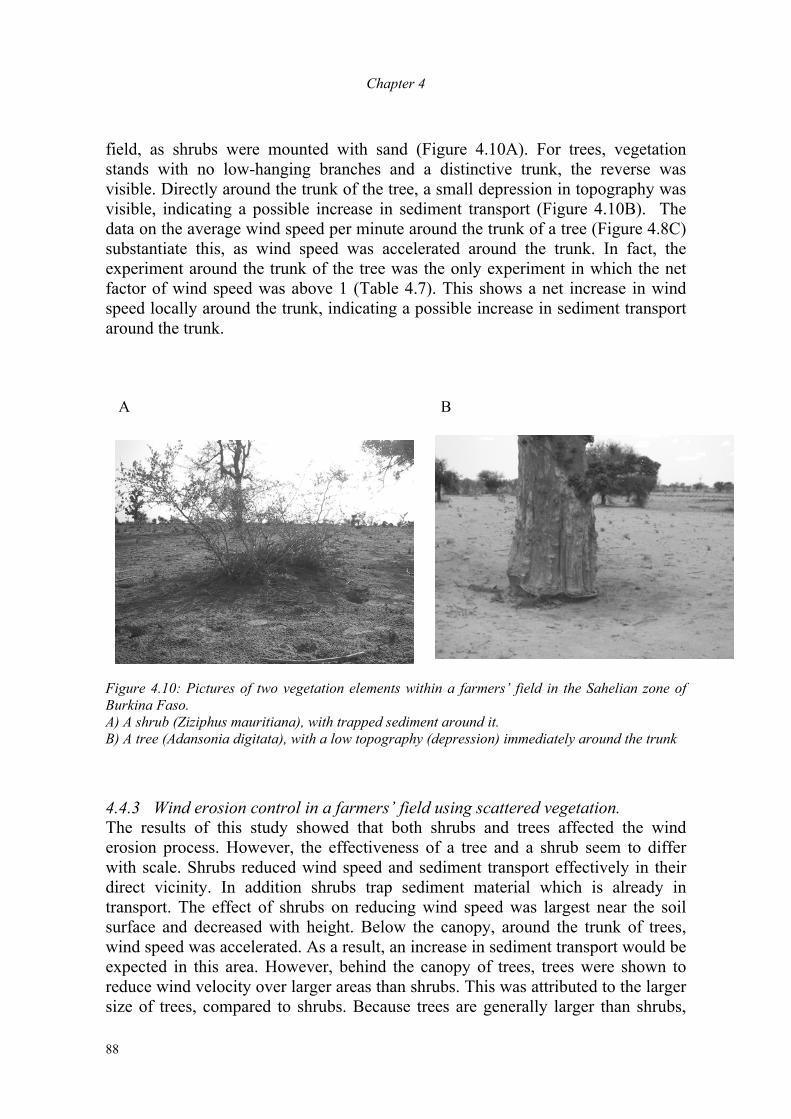
Chapter 4
88
field, as shrubs were mounted with sand (Figure 4.10A). For trees, vegetation stands with no low-hanging branches and a distinctive trunk, the reverse was visible. Directly around the trunk of the tree, a small depression in topography was visible, indicating a possible increase in sediment transport (Figure 4.10B). The data on the average wind speed per minute around the trunk of a tree (Figure 4.8C) substantiate this, as wind speed was accelerated around the trunk. In fact, the experiment around the trunk of the tree was the only experiment in which the net factor of wind speed was above 1 (Table 4.7). This shows a net increase in wind speed locally around the trunk, indicating a possible increase in sediment transport around the trunk.
A B
Figure 4.10: Pictures of two vegetation elements within a farmers’ field in the Sahelian zone of Burkina Faso. A) A shrub (Ziziphus mauritiana), with trapped sediment around it. B) A tree (Adansonia digitata), with a low topography (depression) immediately around the trunk 4.4.3 Wind erosion control in a farmers’ field using scattered vegetation. The results of this study showed that both shrubs and trees affected the wind erosion process. However, the effectiveness of a tree and a shrub seem to differ with scale. Shrubs reduced wind speed and sediment transport effectively in their direct vicinity. In addition shrubs trap sediment material which is already in transport. The effect of shrubs on reducing wind speed was largest near the soil surface and decreased with height. Below the canopy, around the trunk of trees, wind speed was accelerated. As a result, an increase in sediment transport would be expected in this area. However, behind the canopy of trees, trees were shown to reduce wind velocity over larger areas than shrubs. This was attributed to the larger size of trees, compared to shrubs. Because trees are generally larger than shrubs,
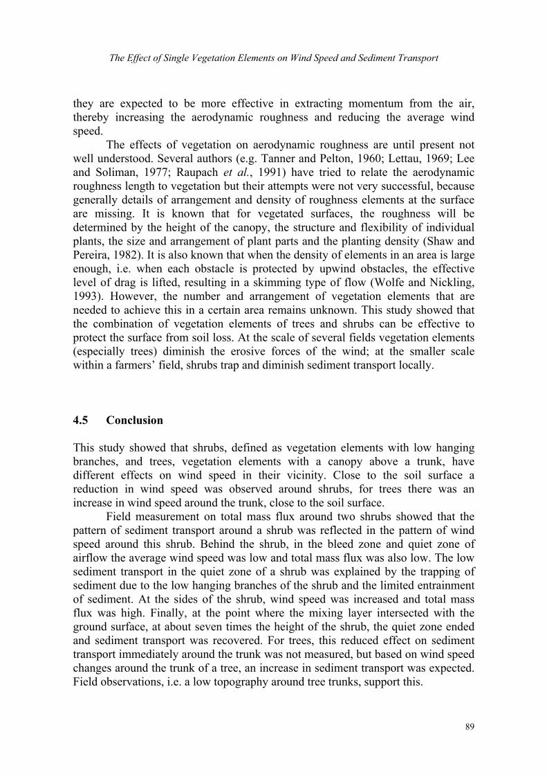
The Effect of Single Vegetation Elements on Wind Speed and Sediment Transport
89
they are expected to be more effective in extracting momentum from the air, thereby increasing the aerodynamic roughness and reducing the average wind speed.
The effects of vegetation on aerodynamic roughness are until present not well understood. Several authors (e.g. Tanner and Pelton, 1960; Lettau, 1969; Lee and Soliman, 1977; Raupach et al., 1991) have tried to relate the aerodynamic roughness length to vegetation but their attempts were not very successful, because generally details of arrangement and density of roughness elements at the surface are missing. It is known that for vegetated surfaces, the roughness will be determined by the height of the canopy, the structure and flexibility of individual plants, the size and arrangement of plant parts and the planting density (Shaw and Pereira, 1982). It is also known that when the density of elements in an area is large enough, i.e. when each obstacle is protected by upwind obstacles, the effective level of drag is lifted, resulting in a skimming type of flow (Wolfe and Nickling, 1993). However, the number and arrangement of vegetation elements that are needed to achieve this in a certain area remains unknown. This study showed that the combination of vegetation elements of trees and shrubs can be effective to protect the surface from soil loss. At the scale of several fields vegetation elements (especially trees) diminish the erosive forces of the wind; at the smaller scale within a farmers’ field, shrubs trap and diminish sediment transport locally. 4.5 Conclusion This study showed that shrubs, defined as vegetation elements with low hanging branches, and trees, vegetation elements with a canopy above a trunk, have different effects on wind speed in their vicinity. Close to the soil surface a reduction in wind speed was observed around shrubs, for trees there was an increase in wind speed around the trunk, close to the soil surface.
Field measurement on total mass flux around two shrubs showed that the pattern of sediment transport around a shrub was reflected in the pattern of wind speed around this shrub. Behind the shrub, in the bleed zone and quiet zone of airflow the average wind speed was low and total mass flux was also low. The low sediment transport in the quiet zone of a shrub was explained by the trapping of sediment due to the low hanging branches of the shrub and the limited entrainment of sediment. At the sides of the shrub, wind speed was increased and total mass flux was high. Finally, at the point where the mixing layer intersected with the ground surface, at about seven times the height of the shrub, the quiet zone ended and sediment transport was recovered. For trees, this reduced effect on sediment transport immediately around the trunk was not measured, but based on wind speed changes around the trunk of a tree, an increase in sediment transport was expected. Field observations, i.e. a low topography around tree trunks, support this.
Chapter 4
90
While shrubs showed a direct impact on soil loss, by trapping and decreasing sediment transport immediately around the vegetation element, their effect on a larger scale, i.e. an increase of the aerodynamic roughness by extracting momentum from the air is expected to be limited because of their size. As trees are generally large objects, trees are expected to be more effective in extracting momentum from the air and reducing the average wind speed in an area than shrubs. Therefore it is concluded that both trees and shrubs are crucial elements of the parkland system, to diminish the erosive forces of the wind. Trees are effective in diminishing the average wind speed and shrubs trap and reduce sediment locally. The amount of trees and shrubs, together with an optimal arrangement of them within a farmers’ field in order to prevent wind erosion adequately demands further research. References Alfaro S.C., Rajot J.L., Nickling W. 2004: Estimation of PM20 emissions by wind erosion: main
sources of uncertainties. Geomorphology 59: 63-74. Bielders C.L., Michels K., Rajot J.L. 2000: On-farm evaluation of ridging and residue
management practices to reduce wind erosion in Niger. Soil Science Society of America Journal 64: 1776-1785.
Bielders C.L., Alvey S., Cronyn N. 2001: Wind erosion: The perspective of grass-roots communities in the Sahel. Land Degradation & Development 12: 57-70.
Cleugh H.A. 1998: Effects of windbreaks on airflow, microclimates and crop yields. Agroforestry Systems 41: 55-84.
Crawley D.M., Nickling W. 2003: Drag partition for regularly-arrayed rough surfaces. Boundary-Layer Meterology 107: 445-468.
Gillette D.A., Stockton P.H. 1989: The effect of nonerodible particles on wind erosion of erodible surface. Journal of Geophysical Research 94: 12885-12893.
Goossens D., Offer Z., London G. 2000: Wind tunnel and field calibration of five aeolian sand traps. Geomorphology 35: 233-252.
Grant P.F., Nickling W.G. 1998: Direct field measurement of wind drag on vegetation for application to windbreak design and modelling. Land Degradation & Development 9: 57-66.
Gross G. 1987: A numerical study of the air flow within an around a single tree. Boundary Layer Meterology 40: 311-327.
Jacobs A.F.G., Van Boxel J.H. 1988a: Changes of the displacement height and roughness length of maize during a growing season. Agricultural and Forest Meteorology 42: 53-62.
Jacobs A.F.G., Van Boxel J.H. 1988b: Computational parameter estimation for a maize crop. Boundary Layer Meteorology 42: 265-279.
Judd M.J., Raupach M.R., Finnigan J.J. 1996: A wind tunnel study of turbulent flow around single and multiple windbreaks. Part I: velocity fields. Boundary Layer Meterology 80: 127-165.
Kaimal J.C., Finnigan J.J. 1994: Atmospheric boundary layer flows, their structure and measurement. Oxford Univ. Press, New York, 289 pp.
Kenny W.A. 1987: A method for estimating windbreak porosity using digitized photographic silhouettes. Agricultural and Forest Meteorology 39: 91-94.
Lamers J.P.A., Michels K., Feil P.R. 1995: Wind erosion control using windbreaks and crop residues: Local knowledge and experimental results. Der Tropenlandwirt, Beiträge zur tropischen Landwirtschaft und Veterinärmedizin 96: 87-96.
The Effect of Single Vegetation Elements on Wind Speed and Sediment Transport
91
Lancaster N., Baas A. 1998: Influence of vegetation cover on sand transport by wind: Field studies at Owens Lake, California. Earth Surface Processes and Landforms 23: 69-82.
Le Houérou H.N. 1997: Climate, flora and fauna changes in the Sahara over the past 500 million years. Journal of Arid Environments 37: 619-647.
Lee B.E., Soliman B.F. 1977: An investigation of the forces on three dimensional bluff bodies in rough wall turbulent boundary layers. Transactions of the ASME, Journal of Fluids Engineering 99: 503-510.
Lee S.J., Park K.C., Park C.W. 2002: Wind tunnel observations about the shelter effect of porous fences on the sand particle movements. Atmospheric Environment 36: 1453-1463.
Leenders J.K., Visser S.M., Stroosnijder L. 2005a: Farmers' perceptions of the role of scattered vegetation in wind erosion control in Burkina Faso. Land Degradation & Development 16: 327-337.
Leenders J.K., Van Boxel J.H., Sterk G. 2005b: Wind forces and related saltation transport in the Sahelian zone of Burkina Faso. Geomorphology 71: 357-752.
Lettau H. 1969: Note on aerodynamic roughness-parameter estimation on the basis of roughness-element description. Journal of Applied Meteorology 8: 828-832.
Marshall J.K. 1971: Drag measurements in roughness arrays of varying density and distribution. Agricultural Meteorology 8: 269-292.
Michels K., Sivakumar M.V.K., Allison B.E. 1995: Wind erosion control using crop residue I. Effects on soil flux and soil properties. Field Crops Res. 40: 101-110.
Mohammed A.E., Stigter C.J., Adam H.S. 1995: Moving sand and its consequences on and near a severely desertified environment and a protective shelterbelt. Arid soil Research and Rehabilitation 9: 423-435.
Morris H.M. 1955: Flow in rough conditions. Transactions of the ASAE 120: 373-398. Musick H.B., Gillette D.A. 1990: Field evaluation of relationships between a vegetation structural
parameter and sheltering against wind erosion. Land Degradation and Rehabilitation 2: 87-94.
Petit S. 2003: Parklands with fodder trees: a Fulbe response to environment and social changes. Applied Geography 23: 205-225.
Raupach M.R., Lu H. 2004: Representation of land-surface processes in aeolian transport models. Environmental Modelling & Software 19: 93 - 112.
Raupach M.R., Antonia R.A., Rajagopalan S. 1991: Rough-wall turbulent boundary layers. Applied Mechanics Reviews 44: 1-25.
Raupach M.R., Gillette D.A., Leys J.F. 1993: The effect of roughness elements on wind erosion threshold. Journal of Geophysical Research-Atmospheres 98: 3023-3029.
Raupach M.R., Woods N., Dorr G., Leys J.F., Cluegh H.A. 2001: The entrapment of particles by windbreaks. Atmospheric Environment 35: 3373 - 3383.
Rinaudo T. 1996: Tailoring wind erosion control methods to farmers' specific needs. pp 161-171. In: B. Buerkert, et al. (Eds.). 'Wind Erosion in West Africa: The Problem and its Control', Germany, 5-7 December 1994. University of Hohenheim.
Ruck V.B., Schmitt F. 1986: Das Strömungsfeld der Einzelbaumuströmung. Abschätzung von Depositionswahrscheinlichkeiten für Feinsttröpfchen. Forstwissenschaftliches Centralblatt 105: 178-196.
Schlichting H. 1936: Experimentelle Untersuchungen zum Rauhigkeitsproblem. Ingen.-Arch 7: 1-34.
Schönfeldt H.J., von Löwis S. 2003: Turbulence-driven saltation in the atmospheric surface layer. Meteorologische Zeitschrift 12: 257-268.
Shao Y. 2000: Physics and modelling of wind erosion. R. Sadourny (Ed.) Atmospheric and Oceanographic Sciences Library, Vol. 23, Kluwer Academic Publishers. Dordrecht, The Netherlands. 393 pp.
Shaw R.H., Pereira A.R. 1982: Aerodynamic roughness of a plant canopy: A numerical experiment. Agricultural Meteorology 26: 61-65.
Chapter 4
92
Sterk G. 1993: Sahelian wind erosion research project, Report III. Description and calibration of sediment samplers. Dep. of Irrigation and Soil & Water Conservation, Wageningen University. Wageningen, The Netherlands.
Sterk G. 2000: Flattened residue effects on wind speed and sediment transport. Soil Science Society of America Journal 64: 852-858.
Sterk G. 2003: Causes, consequences and control of wind erosion in Sahelian Africa: A review. Land Degradation & Development 14: 95-108.
Sterk G., Raats P.A.C. 1996: Comparison of models describing the vertical distribution of wind-eroded sediment. Soil Science Society of America Journal 60: 1914-1919.
Sterk G., Spaan W.P. 1997: Wind erosion control with crop residues in the Sahel. Soil Science Society of America Journal 61: 911-917.
Sterk G., Haigis J. 1998: Farmers' knowledge of wind erosion processes and control methods in Niger. Land Degradation & Development 9: 107-114.
Sterk G., Hermann L., Bationo A. 1996: Wind-blown nutrient transport and soil poductivity changes in southwest Niger. Land Degradation & Development 7: 325-335.
Sterk G., Jacobs A.F.G., Van Boxel J.H. 1998: The effect of turbulent flow structures on saltation transport in the atmospheric boundary layer. Earth Surface Processes and Landforms 23: 877-887.
Stull R.B. 1988: An introduction to boundary layer meteorology. Prentice Hall. Englewood Cliffs, New Jersey. 317 pp.
Tanner C.B., Pelton W.L. 1960: Potential evapotranspiration estimates by the approximate energy balance method of Penman. Journal of Geophysical Research 65: 3391-3413.
Taylor-Powell E. 1991: Integrated management of agricultural watersheds: Land tenure and indigenous knowledge of soil and crop management. Tropical Soils Bulletin 91-04 Texas A&M University: College Station, TX.
Tibke G. 1988: Basic principles of wind erosion control. Agriculture, Ecosystems & Environment 22/23: 103 - 122.
Valentin C. 1995: Sealing, crusting and hardsetting soils in Sahelian agriculture. pp 53-76. In: So HB et al. (Eds). Sealing, Crusting and Hardsetting Soils: Productivity and Conservation. Australian Society of Soil Science, Brisbane, Australia.
van Boxel J.H., Sterk G., Arens S.M. 2004: Sonic anemometers in aeolian sediment transport research. Geomorphology 59: 131-147.
Van de Ven T.A.M., Fryrear D.W., Spaan W.P. 1989: Vegetation characteristics and soil loss by wind. Journal of Soil and Water Conservation 44: 347-349.
Van Dissel S.C., de Graaff J. 1998: Differences between farmers and scientists in the perception of soil erosion: a south African case study. Indigenous Knowledge and Development Monitor 6: 8-9.
Van Gardingen P., Grace J. 1991: Plants and Wind. Advances in Botanical Research 18: 189-253. Visser S.M., Leenders J.K., Leeuwis M. 2003: Farmers' perceptions of erosion by wind and water
in northern Burkina Faso. Land Degradation & Development 14: 123-132. Visser S.M., Sterk G., Snepvangers J.J.J.C. 2004: Spatial variation in wind-blown sediment
transport in geomorphic units in northern Burkina Faso using geostatistical mapping. Geoderma 120: 95-107.
Wilczak J.M., Oncley S.P., Stage S.A. 2000: Sonic anemometer tilt correction algorithms. Boundary-Layer Meteorology 99: 127-150.
Wolfe S.A., Nickling W.G. 1993: The protective role of sparse vegetation in wind erosion. Progress in Physical Geography 17: 50-68.
Wolfe S.A., Nickling W.G. 1996: Shear stress partitioning in sparsely vegetated desert canopies. Earth Surface Processes and Landforms 21: 607-619.


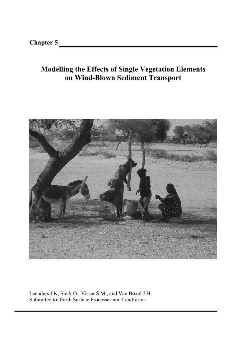
Chapter 5
Modelling the Effects of Single Vegetation Elements on Wind-Blown Sediment Transport
Leenders J.K, Sterk G., Visser S.M., and Van Boxel J.H. Submitted to: Earth Surface Processes and Landforms

Modelling the Effects of Single Vegetation Elements on Wind-Blown Sediment Transport
97
5 Modelling the Effects of Single Vegetation Elements
on Wind-Blown Sediment Transport Abstract Quantification of sediment transport along with the occurrence and the spatial variability of sediment transport at field conditions is a terrain of continuous research. This study is about the modelling of wind-blown sediment transport around a single shrub-type vegetation element. Starting with the selection of a suitable transport equation from four transport equations, the effects of a single vegetation element on wind speed were parameterised. The modified wind speed was then applied to a transport equation to model the change in mass flux around a shrub. The model was tested with field data on wind speed and sediment transport measured around isolated shrubs on a farmer’s field in the north of Burkina Faso.
Of the tested sediment transport equations, a simple empirical equation of Radok (1977) performed best. This was the case for both the entire event duration and for each minute within an event. Uniform values for the empirical constants in the transport equation could not be obtained because of the large variability in soil and roughness characteristics.
The pattern of wind speed and sediment transport around a shrub was modelled by using ellipses to describe the areas of influence behind and on either side of it. The wind speed changed in the lee of the vegetation element depending on its porosity, height and downwind position. Wind speed was recovered to the speed of the approach flow at a downwind distance of 7.5 times the height of the shrub. The variability in wind direction created a “rotating” area of influence around the shrub. The model predicted a 8 % larger reduction in sediment transport in the lee of the vegetation element, and a 22 % larger increase at the sides of it than was observed in field data. 5.1 Introduction Wind-blown sediment transport is a widespread phenomenon in the Sahelian Zone of Africa. It is the cause of many adverse effects. Severe soil degradation can occur as a result of the loss of relatively fertile top soil material (Sterk et al., 1996; Sterk, 2003). Crop damage by abrasion or burial by sand during storms can also occur (Sterk and Haigis, 1998). In addition, it can give rise to health problems due to the occurrence of large amounts of dust in the air (Alfaro et al., 2004) and it can result in sedimentation at undesired places (Mohammed et al., 1995).
Sediment is entrained whenever the force of the wind exceeds the resistance of the soil. When sediment is entrained, the material can be transported in three transport modes: creep, saltation and suspension (Bagnold, 1941). The sand fraction of the sediment (approx. 70 – 1000 µm) is mainly transported in saltation, the bouncing motion of grains. Saltation also initiates the transport of other soil particles. It induces creep, the rolling and sliding of large particles (> 1000 µm) over the surface, and suspension, the raising of fine soil particles (< 70 µm) in the air (Shao, 2000). As wind direction, wind speed and duration of wind erosion
Chapter 5
98
events is variable, the amount of sediment transported in each event is also variable.
The variability of sediment transport is further enhanced by the erodibility of a soil, which also varies in space and time. The erodibility of a soil is determined by several variables such as: soil moisture (Chepil, 1956; Namikas and Sherman, 1995), soil texture (Fryrear et al., 1994), presence of surface crusts (Rice and McEwan, 2001; Goossens, 2004), soil cover (Fryrear, 1985), surface roughness (McKenna Neuman, 1998) and topography (Iversen and Rasmussen, 1999; Sterk et al., 2004). These variables might limit the entrainment of particles in the air and cause sediment transport to be supply-limited. In addition, some of these variables (e.g. soil coverage and surface roughness), might induce trapping of sediment once sediment is entrained and being transported (Raupach et al., 2001).
Modelling is an important tool to understand the process of sediment transport and to develop measures and or strategies to prevent wind erosion. Studies on farmers’ perceptions in Niger and Burkina Faso (Taylor-Powell, 1991; Rinaudo, 1996; Sterk and Haigis, 1998; Bielders et al., 2001; Leenders et al., 2005a) indicated that scattered woody vegetation (trees and shrubs) potentially reduces wind erosion in the Sahel. This was supported by a study on the pattern of sediment transport around a single vegetation element (Leenders et al., 2006). Scattered vegetation reduces sediment transport in three ways: 1) it shelters the soil from the erosive force of the wind by covering a proportion of the surface; 2) it reduces the wind velocity by extracting momentum from the flow; 3) it traps sediment particles (Van de Ven et al., 1989; Wolfe and Nickling, 1993).
The modelling of wind-blown sediment transport around a single vegetation element is an important step towards exploiting and developing strategies of using scattered vegetation to control soil loss. The key in modelling sediment transport is to develop the correct parameterisation of the driving forces of the wind and the erodibility of the soil. Shear stress, expressed by the friction velocity (u*), is used in most sediment transport equations (Greely and Iversen, 1985). Values of the friction velocity are usually obtained from wind speed profiles averaged over periods of at least 10 minutes (Namikas et al., 2003). This way, friction velocity can be obtained by fitting a logarithmic wind profile to the data. But behind an obstacle, wakes generated by roughness elements complicate the flow and the velocity profile departs from the logarithmic wind profile (Raupach et al., 1980). In addition, the process of sediment transport is highly intermittent and characterised by short periods of intense transport and other periods of no or less intense transport. This intermittency is only noticeable at small timescales (part of a second) (Leenders et al., 2005b). It is therefore questionable whether time-averaged, profile-derived estimates of friction velocity are adequate to characterise the wind field for the purpose of sediment transport modelling at small spatial and temporal scales. When wind speed is measured at a high frequency (> 1 Hz), sediment transport correlates well with horizontal wind speed (Sterk et al., 1998; Schönfeldt and Von Löwis, 2003; Leenders et al., 2005b).
Modelling the Effects of Single Vegetation Elements on Wind-Blown Sediment Transport
99
Apart from a distinction between sediment transport models based on friction velocity or wind speed, sediment transport models can also be divided into models that are physically based or empirical. Physically based models try to predict the sediment transport by theoretically describing the processes involved, while empirical models are based on statistical analysis of actual data of wind speed and sediment transport to predict sediment transport. In practice most models are semi-empirical, i.e. a relatively simple theoretical basis combined with empirical equations.
The central issue in modelling sediment transport is to estimate the amount of sediment transported by the wind. At present, however, there is no model that is uniformly valid at a variety of sites (Dong et al., 2003). This is mainly attributed to the deviation of the ideal conditions in wind tunnels, where most transport models were developed, from the field, where ideal conditions usually are absent (Sherman et al., 1998).The ideal conditions related to the wind forces include a unidirectional, fully turbulent, uniform and steady wind and a wind velocity profile that obeys the logarithmic wind profile when sediment is transported. Ideal conditions related to the erodibility of the soil comprise clean, dry and uniformly sized sands and a planar and unobstructed surface (Dong et al., 2003). At the spatial scale of a Sahelian farmer’s field, these ideal conditions are usually not met, due to the presence of a variety of (isolated) vegetation elements. In order to describe sediment transport within an entire field with scattered vegetation, the sediment transport around a single vegetation element needs to be known and modelled first. The aim of this paper, therefore, was to model wind-blown sediment transport around a single vegetation element. Specific objectives were: 1) to select a transport equation that adequately predicts sediment transport; 2) to parameterise the effects of a single vegetation element on wind speed and sediment transport in two dimensions.
5.2 Model concept Two-dimensional modelling of sediment transport around a single vegetation element involves two parameterisations: 1) spatial representation of the areas around a vegetation element in which sediment transport is affected, and 2) quantification of sediment transport within the affected areas. The modelling of sediment transport around single vegetation elements was done by calculating the alteration of wind flow around single vegetation elements. Subsequently the altered wind speed was used to quantify sediment transport around the vegetation element. The model performs these calculations several times during the course of a wind erosion event and is therefore a dynamic model. This was done to capture the variability in wind speed and wind direction during a storm event. The presented model was especially developed for vegetation elements with a canopy starting at the soil surface, which is further referred to as shrubs.
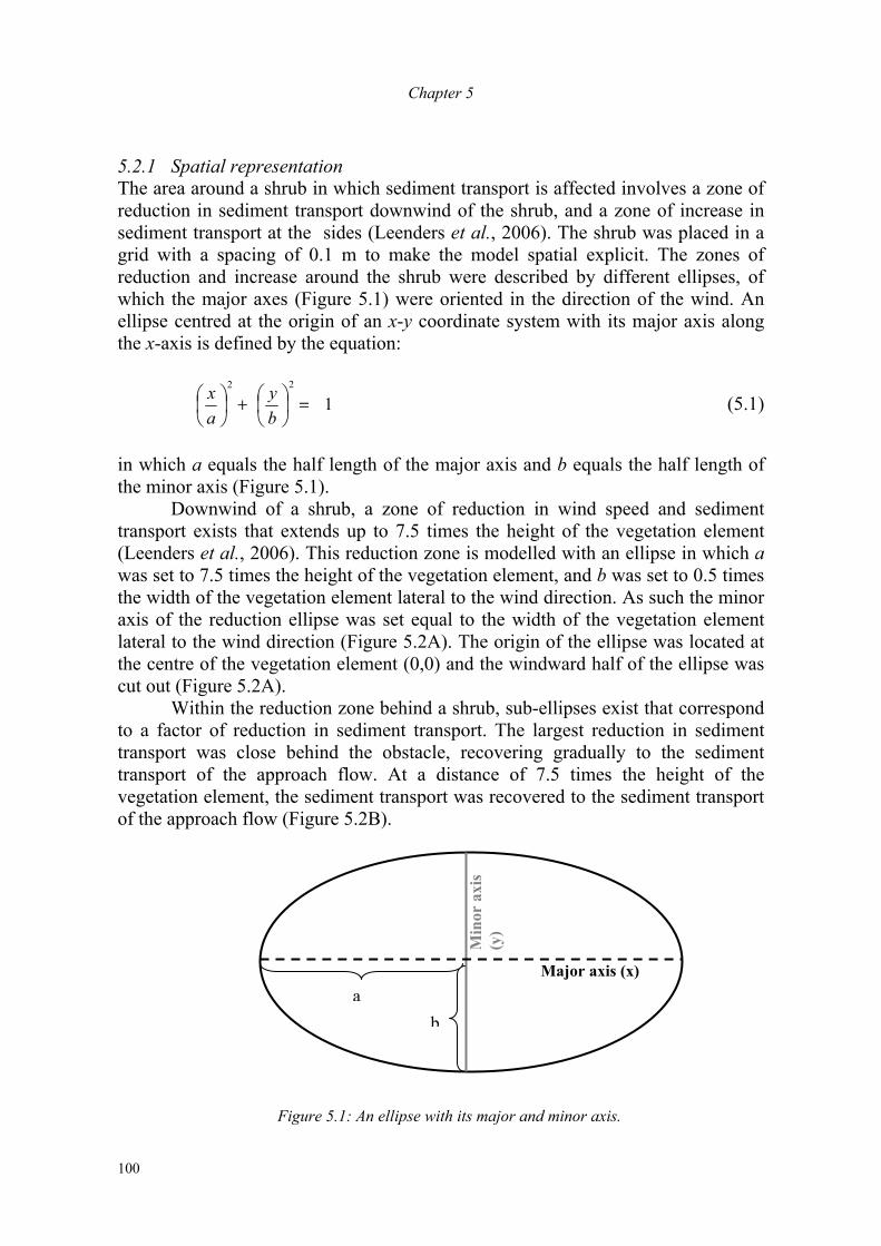
Chapter 5
100
5.2.1 Spatial representation The area around a shrub in which sediment transport is affected involves a zone of reduction in sediment transport downwind of the shrub, and a zone of increase in sediment transport at the sides (Leenders et al., 2006). The shrub was placed in a grid with a spacing of 0.1 m to make the model spatial explicit. The zones of reduction and increase around the shrub were described by different ellipses, of which the major axes (Figure 5.1) were oriented in the direction of the wind. An ellipse centred at the origin of an x-y coordinate system with its major axis along the x-axis is defined by the equation:
122
=⎟⎠⎞
⎜⎝⎛+⎟
⎠⎞
⎜⎝⎛
by
ax (5.1)
in which a equals the half length of the major axis and b equals the half length of the minor axis (Figure 5.1).
Downwind of a shrub, a zone of reduction in wind speed and sediment transport exists that extends up to 7.5 times the height of the vegetation element (Leenders et al., 2006). This reduction zone is modelled with an ellipse in which a was set to 7.5 times the height of the vegetation element, and b was set to 0.5 times the width of the vegetation element lateral to the wind direction. As such the minor axis of the reduction ellipse was set equal to the width of the vegetation element lateral to the wind direction (Figure 5.2A). The origin of the ellipse was located at the centre of the vegetation element (0,0) and the windward half of the ellipse was cut out (Figure 5.2A).
Within the reduction zone behind a shrub, sub-ellipses exist that correspond to a factor of reduction in sediment transport. The largest reduction in sediment transport was close behind the obstacle, recovering gradually to the sediment transport of the approach flow. At a distance of 7.5 times the height of the vegetation element, the sediment transport was recovered to the sediment transport of the approach flow (Figure 5.2B).
Figure 5.1: An ellipse with its major and minor axis.
Major axis (x)
Min
or a
xis
(y)
ba
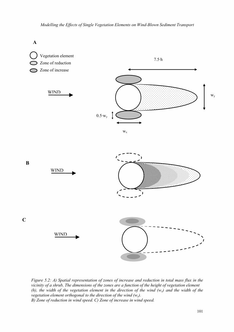
Modelling the Effects of Single Vegetation Elements on Wind-Blown Sediment Transport
101
Figure 5.2: A) Spatial representation of zones of increase and reduction in total mass flux in the vicinity of a shrub, The dimensions of the zones are a function of the height of vegetation element (h), the width of the vegetation element in the direction of the wind (wx) and the width of the vegetation element orthogonal to the direction of the wind (wy). B) Zone of reduction in wind speed. C) Zone of increase in wind speed.
WIND
WIND
wx
wy
7.5·h
0.5·wy
WIND
A
B
C
Vegetation element Zone of reductionZone of increase
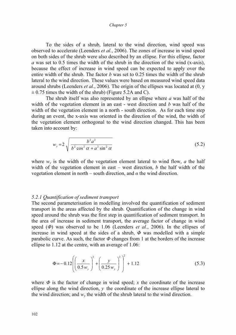
Chapter 5
102
To the sides of a shrub, lateral to the wind direction, wind speed was observed to accelerate (Leenders et al., 2006). The zones of increase in wind speed on both sides of the shrub were also described by an ellipse. For this ellipse, factor a was set to 0.5 times the width of the shrub in the direction of the wind (x-axis), because the effect of increase in wind speed can be expected to apply over the entire width of the shrub. The factor b was set to 0.25 times the width of the shrub lateral to the wind direction. These values were based on measured wind speed data around shrubs (Leenders et al., 2006). The origin of the ellipses was located at (0, y ± 0.75 times the width of the shrub) (Figure 5.2A and C).
The shrub itself was also represented by an ellipse where a was half of the width of the vegetation element in an east - west direction and b was half of the width of the vegetation element in a north - south direction. As for each time step during an event, the x-axis was oriented in the direction of the wind, the width of the vegetation element orthogonal to the wind direction changed. This has been taken into account by:
αα 2222
22
sincos2
ababwy +
= (5.2)
where wy is the width of the vegetation element lateral to wind flow, a the half width of the vegetation element in east – west direction, b the half width of the vegetation element in north – south direction, and α the wind direction. 5.2.1 Quantification of sediment transport The second parameterisation in modelling involved the quantification of sediment transport in the areas affected by the shrub. Quantification of the change in wind speed around the shrub was the first step in quantification of sediment transport. In the area of increase in sediment transport, the average factor of change in wind speed (Φ) was observed to be 1.06 (Leenders et al., 2006). In the ellipses of increase in wind speed at the sides of a shrub, Φ was modelled with a simple parabolic curve. As such, the factor Φ changes from 1 at the borders of the increase ellipse to 1.12 at the centre, with an average of 1.06:
12.125.05.0
12.0
222
+⎟⎟
⎠
⎞
⎜⎜
⎝
⎛
⎟⎟⎠
⎞⎜⎜⎝
⎛+⎟
⎟⎠
⎞⎜⎜⎝
⎛−=Φ
yy wy
wx (5.3)
where Φ is the factor of change in wind speed; x the coordinate of the increase ellipse along the wind direction, y the coordinate of the increase ellipse lateral to the wind direction; and wy the width of the shrub lateral to the wind direction.
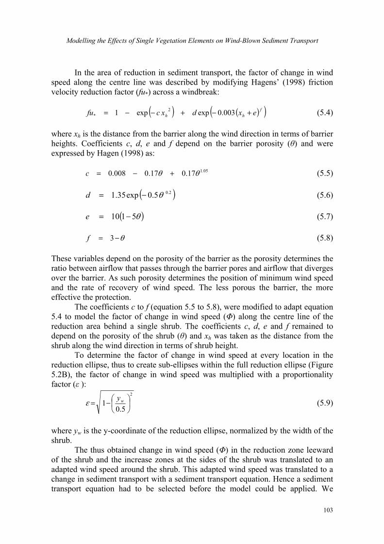
Modelling the Effects of Single Vegetation Elements on Wind-Blown Sediment Transport
103
In the area of reduction in sediment transport, the factor of change in wind speed along the centre line was described by modifying Hagens’ (1998) friction velocity reduction factor (fu*) across a windbreak:
( ) ( )( )f
hh exdxcfu +−+−−= 003.0expexp1 2* (5.4)
where xh is the distance from the barrier along the wind direction in terms of barrier heights. Coefficients c, d, e and f depend on the barrier porosity (θ) and were expressed by Hagen (1998) as:
05.117.017.0008.0 θθ +−=c (5.5)
( )2.05.0exp35.1 θ−=d (5.6)
( )θ5110 −=e (5.7)
θ−= 3f (5.8) These variables depend on the porosity of the barrier as the porosity determines the ratio between airflow that passes through the barrier pores and airflow that diverges over the barrier. As such porosity determines the position of minimum wind speed and the rate of recovery of wind speed. The less porous the barrier, the more effective the protection.
The coefficients c to f (equation 5.5 to 5.8), were modified to adapt equation 5.4 to model the factor of change in wind speed (Φ) along the centre line of the reduction area behind a single shrub. The coefficients c, d, e and f remained to depend on the porosity of the shrub (θ) and xh was taken as the distance from the shrub along the wind direction in terms of shrub height.
To determine the factor of change in wind speed at every location in the reduction ellipse, thus to create sub-ellipses within the full reduction ellipse (Figure 5.2B), the factor of change in wind speed was multiplied with a proportionality factor (ε ):
2
5.01 ⎟
⎠⎞
⎜⎝⎛−= wyε (5.9)
where yw is the y-coordinate of the reduction ellipse, normalized by the width of the shrub.
The thus obtained change in wind speed (Φ) in the reduction zone leeward of the shrub and the increase zones at the sides of the shrub was translated to an adapted wind speed around the shrub. This adapted wind speed was translated to a change in sediment transport with a sediment transport equation. Hence a sediment transport equation had to be selected before the model could be applied. We
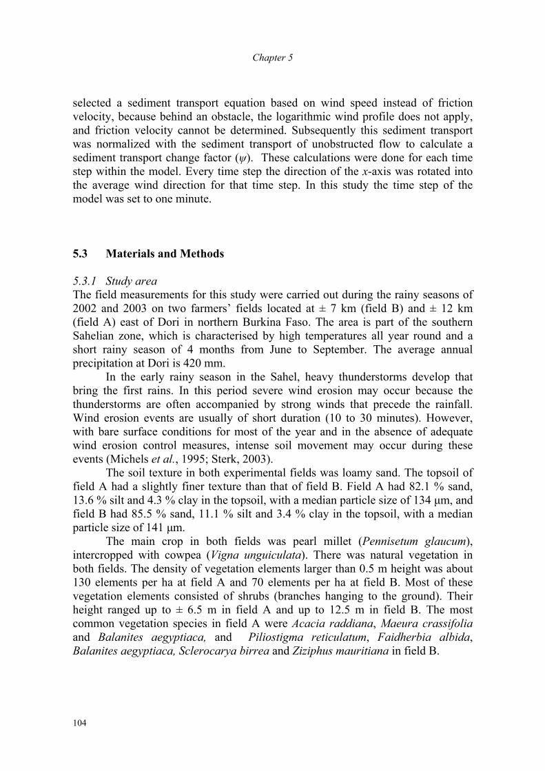
Chapter 5
104
selected a sediment transport equation based on wind speed instead of friction velocity, because behind an obstacle, the logarithmic wind profile does not apply, and friction velocity cannot be determined. Subsequently this sediment transport was normalized with the sediment transport of unobstructed flow to calculate a sediment transport change factor (ψ). These calculations were done for each time step within the model. Every time step the direction of the x-axis was rotated into the average wind direction for that time step. In this study the time step of the model was set to one minute.
5.3 Materials and Methods 5.3.1 Study area The field measurements for this study were carried out during the rainy seasons of 2002 and 2003 on two farmers’ fields located at ± 7 km (field B) and ± 12 km (field A) east of Dori in northern Burkina Faso. The area is part of the southern Sahelian zone, which is characterised by high temperatures all year round and a short rainy season of 4 months from June to September. The average annual precipitation at Dori is 420 mm.
In the early rainy season in the Sahel, heavy thunderstorms develop that bring the first rains. In this period severe wind erosion may occur because the thunderstorms are often accompanied by strong winds that precede the rainfall. Wind erosion events are usually of short duration (10 to 30 minutes). However, with bare surface conditions for most of the year and in the absence of adequate wind erosion control measures, intense soil movement may occur during these events (Michels et al., 1995; Sterk, 2003).
The soil texture in both experimental fields was loamy sand. The topsoil of field A had a slightly finer texture than that of field B. Field A had 82.1 % sand, 13.6 % silt and 4.3 % clay in the topsoil, with a median particle size of 134 µm, and field B had 85.5 % sand, 11.1 % silt and 3.4 % clay in the topsoil, with a median particle size of 141 µm.
The main crop in both fields was pearl millet (Pennisetum glaucum), intercropped with cowpea (Vigna unguiculata). There was natural vegetation in both fields. The density of vegetation elements larger than 0.5 m height was about 130 elements per ha at field A and 70 elements per ha at field B. Most of these vegetation elements consisted of shrubs (branches hanging to the ground). Their height ranged up to ± 6.5 m in field A and up to 12.5 m in field B. The most common vegetation species in field A were Acacia raddiana, Maeura crassifolia and Balanites aegyptiaca, and Piliostigma reticulatum, Faidherbia albida, Balanites aegyptiaca, Sclerocarya birrea and Ziziphus mauritiana in field B.
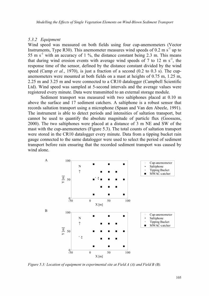
Modelling the Effects of Single Vegetation Elements on Wind-Blown Sediment Transport
105
5.3.2 Equipment Wind speed was measured on both fields using four cup-anemometers (Vector Instruments, Type R30). This anemometer measures wind speeds of 0.2 m s-1 up to 55 m s-1 with an accuracy of 1 %, the distance constant being 2.3 m. This means that during wind erosion events with average wind speeds of 7 to 12 m s-1, the response time of the sensor, defined by the distance constant divided by the wind speed (Camp et al., 1970), is just a fraction of a second (0.2 to 0.3 s). The cup-anemometers were mounted at both fields on a mast at heights of 0.75 m, 1.25 m, 2.25 m and 3.25 m and were connected to a CR10 datalogger (Campbell Scientific Ltd). Wind speed was sampled at 5-second intervals and the average values were registered every minute. Data were transmitted to an external storage module.
Sediment transport was measured with two saltiphones placed at 0.10 m above the surface and 17 sediment catchers. A saltiphone is a robust sensor that records saltation transport using a microphone (Spaan and Van den Abeele, 1991). The instrument is able to detect periods and intensities of saltation transport, but cannot be used to quantify the absolute magnitude of particle flux (Goossens, 2000). The two saltiphones were placed at a distance of 3 m NE and SW of the mast with the cup-anemometers (Figure 5.3). The total counts of saltation transport were stored in the CR10 datalogger every minute. Data from a tipping bucket rain gauge connected to the same datalogger were used to select the period of sediment transport before rain ensuring that the recorded sediment transport was caused by wind alone.
-50 0 50 1000
50
100
↑
N
X [m]
Y [m
]
Cup-anemometerSaltiphoneTipping BucketMWAC-catcher
-50 0 50 1000
50
100
↑
N
X [m]
Y [m
]
Cup-anemometerSaltiphoneTipping BucketMWAC-catcher
A
B
Figure 5.3: Location of equipment in experimental site at Field A (A) and Field B (B).
Chapter 5
106
The total particle flux during a storm was measured with Modified Wilson and Cooke (MWAC) catchers, which trap moving material across height. The traps consist of a plastic bottle with an inlet and an outlet glass tube entering the bottle through the cap. The internal diameter of the inlet and outlet glass tubes measures 8 mm making the opening of the glass tube 50.3 mm2. Traps are mounted horizontally on a mast. A wind vane connected to the mast ensures that the inlet tubes are pointed into the wind. Sediment transported in the air enters the inlet glass tube along with the air and settles in the sample bottle. The air escapes through the outlet glass tube. The MWAC catchers used in this study measured sediment transport at five heights. The intended measuring heights were 0.05, 0.12, 0.19, 0.26 and 0.75 metres above the soil surface, but these values could change up to 20 mm because of soil surface changes during storms. For more details on the MWAC catcher see Sterk and Raats (1996). 5.3.3 Calculation of transported mass Mean horizontal mass flux densities q(z) (kg m-2 s-1) at height z (m) were calculated from the weights of the trapped materials and the event duration. Subsequently, a mass flux density profile was fitted through the measured mass flux densities to calculate the total mass flux Q (kg m-1 s-1). For this purpose, a combined model was used to describe the mass flux densities (Sterk et al., 1996). This model was found to be more accurate than a modified power function as suggested by Zingg (1953). The equation of the combined mass flux model is given by:
)exp()1()(γβznzkzq m −++= − (5.10)
where q(z) is the mass flux density (kg m-2 s-1) at height z (m); and k, m and n are regression coefficients. The coefficient m is dimensionless while the coefficients k and n have the dimensions of mass flux density (kg m-2 s-1); the length scales β and γ were taken as 1 m in this study. An extensive description of the model and the fitting method can be found in Sterk and Raats (1996).
The fitted mass flux density profile was integrated over height from 0 to 1m, to calculate the mass flux at the sampling location (kg m-1 s-1) up to 1 m above the soil surface. The total mass flux, Qt (kg m-1 s-1), was obtained by dividing Q by the trapping efficiency of the catcher. But, there is some debate on the trapping efficiency of the MWAC catcher. Sterk (1993) found an overall trapping efficiency of the MWAC catcher of 0.49 with a standard deviation of 0.03. This was based on 12 runs in a wind tunnel with wind speeds ranging from 9.9 to 11.5 m s-1 using Sahelian sand. A comparable efficiency (0.51) was found by Cornelis et al. (2004). Goossens et al. (2000) obtained an overall efficiency twice as high, based on 15 runs in a wind tunnel with wind speeds ranging from 6.6 to 14.4 ms-1. The efficiency measured by Goossens et al. (2000) varied from 0.7 – 1.2, depending on
Modelling the Effects of Single Vegetation Elements on Wind-Blown Sediment Transport
107
sediment size and wind speed. The method to determine the efficiency of the catcher in these studies differed. Sterk (1993) and Cornelis et al. (2004) used the entire catcher, whereas Goossens et al. (2000) only used one sediment trap. Another possibility to explain the smaller trapping efficiency of Sterk (1993) might be an underestimation of the predicted amount of sediment transport by equation 5.10 close to the surface compared to other mass transport equations (e.g. Stout and Zobeck (1996)). In our study an efficiency of 0.49 was used because we applied the same equation as Sterk (1993) and because this efficiency was determined by using Sahelian sand. In addition the efficiency of 0.49 was supported by the study of Cornelis et al., (2004). 5.3.4 Fit of transport equations Four transport equations were used to fit the measured total mass fluxes (Qt) to wind characteristics (Table 5.1). These were the transport equations of O’Brien and Rindlaub (1936); Kuhlman (1958); Radok (1977); and Dong et al. (2003). The model of Radok (1977) is the only fully empirical model in the list, the others have relatively sound theoretical support (Dong et al., 2003). Radok’s model (1977) and the model of Kuhlman (1958) have the limitation that they can predict sediment transport even when wind velocity is below threshold. Therefore these models should only be applied when wind velocity is above the threshold wind velocity for sediment transport. For the models of Kuhlman (1958) and Dong et al., (2003) this problem is solved by introducing a threshold velocity. The threshold wind velocity at both fields was set to 6 m s-1 at a height of 3.25 m.
The performance of the four transport models was tested at experimental site B for the storm events of the rainy season in 2003. The equations of Table 5.1 were fitted to find optimum values for the empirical constants and thus an optimum goodness of fit. The wind speed measured at 3.25 m height, together with the median of the measured total mass flux was used for the curve fitting. First, a curve fitting was done for the median of the total mass flux that was observed in the entire event. Second, the transport models were fitted to the measured total mass flux per minute for each minute within an event. These one-minute total mass fluxes were determined by multiplying the total mass flux Qt (kg m-1 s-1) with the fraction of saltation transport for each minute. This fraction was taken as the number of hits that was registered by the saltiphone for each minute divided by the total number of hits registered during the event. The performance of the best overall fit of the transport equations was validated by applying it at site A for the events in 2003.
Chapter 5
108
Table 5.1: Overview of the transport models used in this study (after Dong et al., 2003).
Contributor Expression Equation
O’Brien and Rindlaub (1936) Q = C1 (ρ/g) u3 (5.11)
Kuhlman (1958) Q = C2 (1-Ru3) (ρ/g) u3 (5.12)
Radok (1977) Q = A etu (5.13)
Dong et al. (2003) Q = C3 (1-Ru)2 (ρ/g) u3 (5.14)
Q = mass flux [kg m-1 s-1 ]; C1-3 = constant [-];ρ = air density [kg m-3]; g = acceleration due to gravity [m s-2]; u = wind velocity [m s-1]; Ru = ut/u: threshold wind velocity/wind velocity [-]; A = empirical constant [kg m-1 s-1 ]; t = empirical constant [s m-1 ]. 5.3.5 Modelling sediment transport around a shrub The change in wind speed was modelled downwind of two shrubs at experimental site B: a Hyphaene thebaica of 0.6 m height and a Commiphora africana of 1.9 m height (Figure 5.4). The optical porosity (θ) of H. thebaica and C. africana was 18 % and 79 %, respectively. It was determined by digital photogrammetry, similar to the method used by Kenney (1987). A digital photo of part of the canopy was taken at approximately 25 cm from the canopy with a Canon IXUS Digital camera with a resolution of 2.1M pixels and turned into black and white. The threshold value to turn pixels into black or white was visually determined. The percentage of white pixels in the photo was taken as the porosity of the canopy. This value of porosity is the optical porosity, which is not the same as the volumetric porosity. Optical porosity is generally an underestimation of volumetric porosity because much of the small-scale porosity (between leaves and branches) is beyond the resolution of analysis and the vegetation element obscures transmission of light through it (Grant and Nickling, 1998).
First, the coefficients c, d, e and f (equation 5.5-5.8) were adapted to model the factor of change in wind speed (Φ) along the centre line of the reduction area behind a shrub. This was done by fitting equation 5.4 to data that were obtained from two experiments on the change of wind speed measured around the H. thebaica (Leenders et al., 2006). These datasets were obtained at 0.40 m above the soil surface. One of the datasets was obtained with an average wind speed of 2.8 m s-1, the other with an average wind speed of 4.2 m s-1 at 0.40 m. The datasets comprised of 436 and 450 observations of average wind speed per minute, normalized with upwind average wind speed per minute at different locations around the shrub. As such these observation points represent the factor of change in wind speed (Φ) around a shrub. The observation points were interpolated to a grid with spacing of 0.1 m with a triangle-based linear interpolation (Leenders et al., 2006). The thus fitted coefficients of c to f were tested with a dataset of changes in wind speed around the C. africana. This dataset was obtained at 0.45 m height, with an average wind speed of 3.85 m s-1 at 0.45 m above the soil surface. It
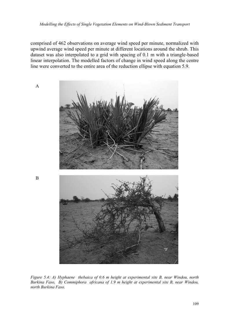
Modelling the Effects of Single Vegetation Elements on Wind-Blown Sediment Transport
109
comprised of 462 observations on average wind speed per minute, normalized with upwind average wind speed per minute at different locations around the shrub. This dataset was also interpolated to a grid with spacing of 0.1 m with a triangle-based linear interpolation. The modelled factors of change in wind speed along the centre line were converted to the entire area of the reduction ellipse with equation 5.9.
Figure 5.4: A) Hyphaene thebaica of 0.6 m height at experimental site B, near Windou, north Burkina Faso, B) Commiphora africana of 1.9 m height at experimental site B, near Windou, north Burkina Faso.
A
B
Chapter 5
110
Second, the developed model to simulate changes in sediment transport around a shrub was run for the events of 2002 around the H. thebaica. It was validated with the total mass fluxes around the H. thebaica that were measured during the rainy season of 2002 (Leenders et al., 2006). This comprised data of 54 observation points on changes in total mass flux at different locations around the H. thebaica. These observations were interpolated to a grid with spacing of 0.1 m with a triangle-based linear interpolation (Leenders et al., 2006).
5.4 Results 5.4.1 Fit of transport equations During the rainy season of 2003, a total of 10 events with sediment transport occurred at both fields. Two events were of very low intensity and lasted only a few minutes. At both fields the record of one event was incomplete due to malfunctioning of the saltiphone. As a result data from 7 events were used in the analysis.
The variability among the events was large (Table 5.2). Some events lasted less than 30 minutes whereas others lasted more than an hour. The average wind direction as well as the mean wind velocity varied considerably. In addition, wind velocity and wind direction differed during an event. For example, in the event of 27 May on experimental site A, both wind velocity and wind direction had a larger variability than during the event of 8 July on the same experimental site. Average wind velocity, wind direction and duration of an event changed per experimental site as well. This indicates the local character of events. The event of 4 June for example did only occur at experimental site B while the event of 24 June was only observed at experimental site A. (Table 5.2). At experimental site A, the wind velocities of the events were generally lower than at experimental site B. This was explained by the presence of more vegetation elements at site A compared to site B.
The observed total mass fluxes at the two experimental sites (Figure 5.5) were of the same order of magnitude as those observed by Sterk and Raats (1996) in the South of Niger. Measured total mass flux varied from event to event, even when event characteristics were similar. For example, at experimental site A, the observed sediment transport during the events of 27 May and 1 July differed (Figure 5.5A), while characteristics of the events were similar (Table 5.2A). The difference in measured total mass flux for these events was probably related to the increased roughness due to the crop canopy. Experimental site A was sown on 29 May, thus on 27 May the soil surface was still bare, whereas on 1 July a crop was present. The range in total mass flux that was observed in the 17 MWAC catchers for a single event could be large (e.g. the event of 26 June at experimental site A) (Figure 5.5A). This indicates the high spatial variability in total mass fluxes, which was also observed by Sterk and Stein (1997) and Visser et al. (2004). In addition to the variability in mass flux within the experimental plots, mass fluxes varied also
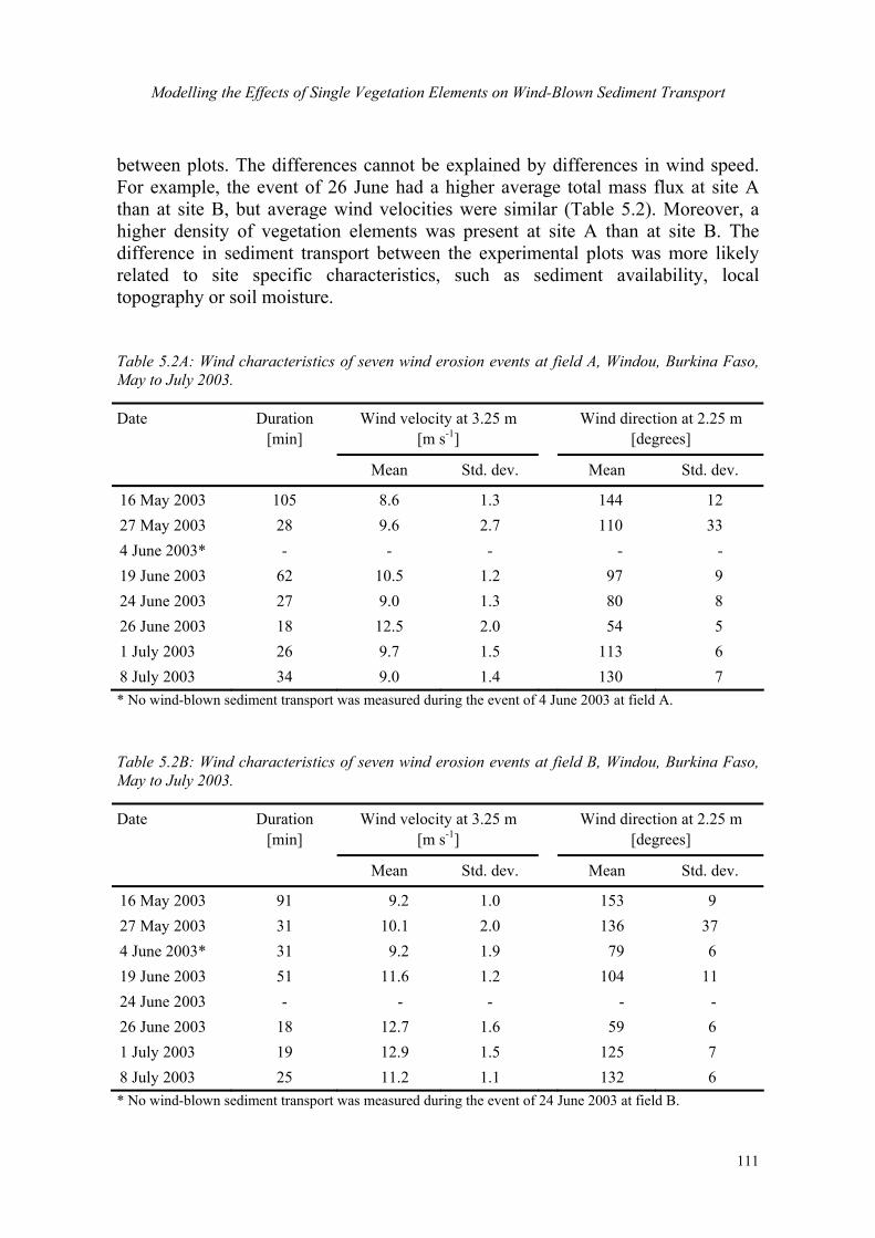
Modelling the Effects of Single Vegetation Elements on Wind-Blown Sediment Transport
111
between plots. The differences cannot be explained by differences in wind speed. For example, the event of 26 June had a higher average total mass flux at site A than at site B, but average wind velocities were similar (Table 5.2). Moreover, a higher density of vegetation elements was present at site A than at site B. The difference in sediment transport between the experimental plots was more likely related to site specific characteristics, such as sediment availability, local topography or soil moisture.
Table 5.2A: Wind characteristics of seven wind erosion events at field A, Windou, Burkina Faso, May to July 2003.
Date Duration [min]
Wind velocity at 3.25 m [m s-1]
Wind direction at 2.25 m [degrees]
Mean Std. dev. Mean Std. dev.
16 May 2003 105 8.6 1.3 144 12 27 May 2003 28 9.6 2.7 110 33 4 June 2003* - - - - - 19 June 2003 62 10.5 1.2 97 9 24 June 2003 27 9.0 1.3 80 8 26 June 2003 18 12.5 2.0 54 5 1 July 2003 26 9.7 1.5 113 6 8 July 2003 34 9.0 1.4 130 7 * No wind-blown sediment transport was measured during the event of 4 June 2003 at field A.
Table 5.2B: Wind characteristics of seven wind erosion events at field B, Windou, Burkina Faso, May to July 2003.
Date Duration [min]
Wind velocity at 3.25 m [m s-1]
Wind direction at 2.25 m [degrees]
Mean Std. dev. Mean Std. dev.
16 May 2003 91 9.2 1.0 153 9 27 May 2003 31 10.1 2.0 136 37 4 June 2003* 31 9.2 1.9 79 6 19 June 2003 51 11.6 1.2 104 11 24 June 2003 - - - - - 26 June 2003 18 12.7 1.6 59 6 1 July 2003 19 12.9 1.5 125 7 8 July 2003 25 11.2 1.1 132 6 * No wind-blown sediment transport was measured during the event of 24 June 2003 at field B.
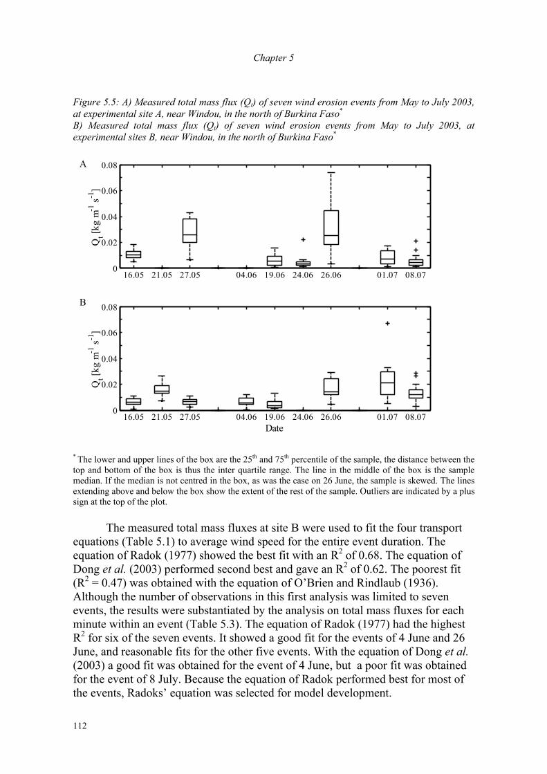
Chapter 5
112
Figure 5.5: A) Measured total mass flux (Qt) of seven wind erosion events from May to July 2003, at experimental site A, near Windou, in the north of Burkina Faso* B) Measured total mass flux (Qt) of seven wind erosion events from May to July 2003, at experimental sites B, near Windou, in the north of Burkina Faso*
16.05 21.05 27.05 04.06 19.06 24.06 26.06 01.07 08.070
0.02
0.04
0.06
0.08
Qt [k
g m-1
s-1
]
16.05 21.05 27.05 04.06 19.06 24.06 26.06 01.07 08.070
0.02
0.04
0.06
0.08
Qt [k
g m-1
s-1
]
Date
A
B
* The lower and upper lines of the box are the 25th and 75th percentile of the sample, the distance between the top and bottom of the box is thus the inter quartile range. The line in the middle of the box is the sample median. If the median is not centred in the box, as was the case on 26 June, the sample is skewed. The lines extending above and below the box show the extent of the rest of the sample. Outliers are indicated by a plus sign at the top of the plot. The measured total mass fluxes at site B were used to fit the four transport equations (Table 5.1) to average wind speed for the entire event duration. The equation of Radok (1977) showed the best fit with an R2 of 0.68. The equation of Dong et al. (2003) performed second best and gave an R2 of 0.62. The poorest fit (R2 = 0.47) was obtained with the equation of O’Brien and Rindlaub (1936). Although the number of observations in this first analysis was limited to seven events, the results were substantiated by the analysis on total mass fluxes for each minute within an event (Table 5.3). The equation of Radok (1977) had the highest R2 for six of the seven events. It showed a good fit for the events of 4 June and 26 June, and reasonable fits for the other five events. With the equation of Dong et al. (2003) a good fit was obtained for the event of 4 June, but a poor fit was obtained for the event of 8 July. Because the equation of Radok performed best for most of the events, Radoks’ equation was selected for model development.

Modelling the Effects of Single Vegetation Elements on Wind-Blown Sediment Transport
113
Table 5.3: Best fit of total mass flux per minute to four transport equations for seven storm events at field B, Windou, north Burkina Faso.
Date
n
[min]
R2 O’Brien and Rindlaub
(eq. 5.11)
R2 Kuhlman (eq. 5.12)
R2 Radok
(eq. 5.13)
R2 Dong et al (eq. 5.14)
16 May 2003 91 0.27 0.30 0.51 0.55
27 May 2003 31 0.40 0.43 0.48 0.37
4 June 2003 31 0.53 0.57 0.78 0.73
19 June 2003 51 0.19 0.20 0.44 0.37
26 June 2003 18 0.28 0.31 0.82 0.36
1 July 2003 19 0.30 0.30 0.49 0.31
8 July 2003 25 0.16 0.16 0.43 0.17
Although the equation of Radok (1977) best fitted the data of both the entire
event duration as well as the one-minute data during an event, the empirical constants A and t differed per fit (Table 5.4). The constants, however, seemed to be related: when A was plotted against t, a fit of an exponential curve through the data explained the variance in A for 82%. Therefore, the sediment transport data of each minute within an event were also fitted to the equation of Radok (1977) by fixing the empirical constant t to 0.7 for each event (Table 5.4). The value of 0.7 was chosen because it was the average of the fitted values of t, for all events at experimental site B using both saltiphones. The resulting R2-values were comparable to those obtained through an optimal fit of both A and t. A constant value for A, that would represent the soil conditions during the event, keeping t fixed to 0.7, was not obtained. This was attributed to the variability of soil characteristics (e.g. soil moisture, crusting and crop growth) during the season. However, with the exception of the event of 4 June, the constant A showed an increasing trend during the growing season (Table 5.4). This seems logical as the resistance of the soil to entrainment is expected to increase during the growing season because of an increased crop canopy. The deviation of the A-value of 4 June might be related to an increased sediment availability because field B was entirely hoed when the site was sown on 27 May.

Chapter 5
114
Table 5.4:Empirical constants A and t for each event in 2003 at field B, together with goodness of fit for the optimal fit and in case of t = 0.7 s m-1.
Date Optimal fit A and t Best fit A, t = 0.7 [s m-1]
A [kg m-1 s-1]
t [s m-1]
R2 [%]
A [kg m-1 s-1]
R2 [%]
16 May 2003 9.65E-09 0.92 0.51 8.54E-08 0.48
27 May 2003 5.51E-06 0.35 0.48 2.86E-08 0.12
4 June 2003 2.03E-07 0.67 0.78 1.09E-07 0.78
19 June 2003 1.04E-08 0.74 0.44 1.36E-08 0.42
26 June 2003 2.09E-07 0.62 0.82 4.77E-08 0.81
1 July 2003 1.51E-06 0.50 0.49 2.27E-07 0.47
8 July 2003 3.40E-07 0.64 0.43 3.83E-07 0.39
Radok’s model (1977) was tested with the sediment transport data of site A
by using the values of the constants A and t, from field B for each event. The constant A of site B was adjusted by dividing it by 2 to take the larger number of vegetation elements of site A into account (about twice as much). The resulting R2-values were low. Two of the seven events, those on 16 May and 8 July, showed a moderate fit of mass flux data, the R2 was 0.49 for both events. The event of 27 May showed a poor fit with an R2 of 0.25. For the rest of the events the fit even fell out of the range of the dataset, which was shown by a residual sum of squares being larger than the total sum of squares. These results show that standard transport equations developed in a wind tunnel always need to be adapted to the ”site-specific” field situation. In order to develop, calibrate and validate a sediment transport equation, good quality data on sediment transport, wind and soil characteristics are required. This means, that either the soil characteristics need to be determined closely to grasp the spatial and temporal variability in the field, or measurements on sediment transport need to be done to adapt and calibrate existing models. It was further shown that this adaptation should be done for each event separately. 5.4.2 Modelling sediment transport around a single vegetation element Figure 5.6 shows the interpolated wind speed data at the centre line downwind of the H. thebaica and C. Africana that were obtained from the dataset of wind speed measurements around shrubs (Leenders et al., 2006). The figure shows the effect of porosity and downwind distance from the shrub on the reduction of wind speed. The two experiments around the H. thebaica showed similar results. The H.
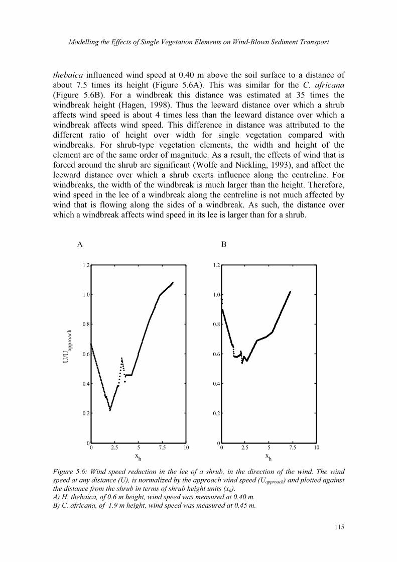
Modelling the Effects of Single Vegetation Elements on Wind-Blown Sediment Transport
115
thebaica influenced wind speed at 0.40 m above the soil surface to a distance of about 7.5 times its height (Figure 5.6A). This was similar for the C. africana (Figure 5.6B). For a windbreak this distance was estimated at 35 times the windbreak height (Hagen, 1998). Thus the leeward distance over which a shrub affects wind speed is about 4 times less than the leeward distance over which a windbreak affects wind speed. This difference in distance was attributed to the different ratio of height over width for single vegetation compared with windbreaks. For shrub-type vegetation elements, the width and height of the element are of the same order of magnitude. As a result, the effects of wind that is forced around the shrub are significant (Wolfe and Nickling, 1993), and affect the leeward distance over which a shrub exerts influence along the centreline. For windbreaks, the width of the windbreak is much larger than the height. Therefore, wind speed in the lee of a windbreak along the centreline is not much affected by wind that is flowing along the sides of a windbreak. As such, the distance over which a windbreak affects wind speed in its lee is larger than for a shrub. A B
0 2.5 5 7.5 100
0.2
0.4
0.6
0.8
1.0
1.2
xh
U/U
appr
oach
0 2.5 5 7.5 100
0.2
0.4
0.6
0.8
1.0
1.2
xh
Figure 5.6: Wind speed reduction in the lee of a shrub, in the direction of the wind. The wind speed at any distance (U), is normalized by the approach wind speed (Uapproach) and plotted against the distance from the shrub in terms of shrub height units (xh). A) H. thebaica, of 0.6 m height, wind speed was measured at 0.40 m. B) C. africana, of 1.9 m height, wind speed was measured at 0.45 m.
Chapter 5
116
The reduction in wind speed behind the C. Africana was less than behind the H. thebaica (Figure 5.6). This was attributed to the higher (optical) porosity of the C. africana (79 %) compared to the H. thebaica (18 %). The interpolated wind speed data at the centreline downwind of the H. thebaica as shown in Figure 5.6A were used to modify the coefficients c, d, e and f of equation 4 for a shrub-type vegetation element. This resulted in:
( )05.117.017.0008.013 θθ +−=c (5.15)
( )2.05.0exp05.1 θ−=d (5.16)
( )θ5.015.2 −=e (5.17)
θ−= 5f (5.18)
where θ is the porosity of the vegetation element.
The validity of the coefficients c to f, as expressed in equation (5.15) to (5.18), was tested with the dataset along the centreline behind the C. Africana (Figure 5.6B). Using the coefficients c to f calculated from equation 5.15 to 5.18 in equation 5.4, predicted an average reduction in wind speed of 23 % along the centre line downwind of the C. africana. In the dataset of (Leenders et al., 2006) a reduction in wind speed of 27 % was measured behind the C. africana. The modelled reduction in wind speed underestimated the observed reduction, but the values are in reasonable agreement. With the calculated values for reduction in wind speed on the centreline downwind of a shrub an adapted wind speed was calculated, which was used in the Radok equation to calculate the change in total mass flux. A typical pattern of the factor of reduction in wind speed (Φ) and total mass flux (ψ) in the lee of a shrub is shown in Figure 5.7. In the immediate lee of the shrub, sediment transport is limited, and it gradually recovers to an undisturbed total mass flux (ψ = 1) at a distance of 7.5 times the height of the vegetation element. When modelling all the events of 2002 an average reduction in total mass flux of 58 % was modelled along the centre line behind the H. thebaica. The reduction in measured mass flux along the centre line behind this element was 53 %. The difference between predicted and observed sediment transport was thus only 5 %. The modelled reduction in mass flux along the centre line overestimated the observed reduction, but the values are in reasonable agreement. For the entire area of reduction downwind of the H. thebaica, the difference between measured total mass flux and modelled total mass flux was 8 %. The model predicted a reduction of 57 % in total mass flux in the reduction zone, whereas a reduction of 49 % was derived from measurements. Also for the entire reduction zone, the modelled reduction in mass flux was overestimated, but the values are in reasonable agreement.
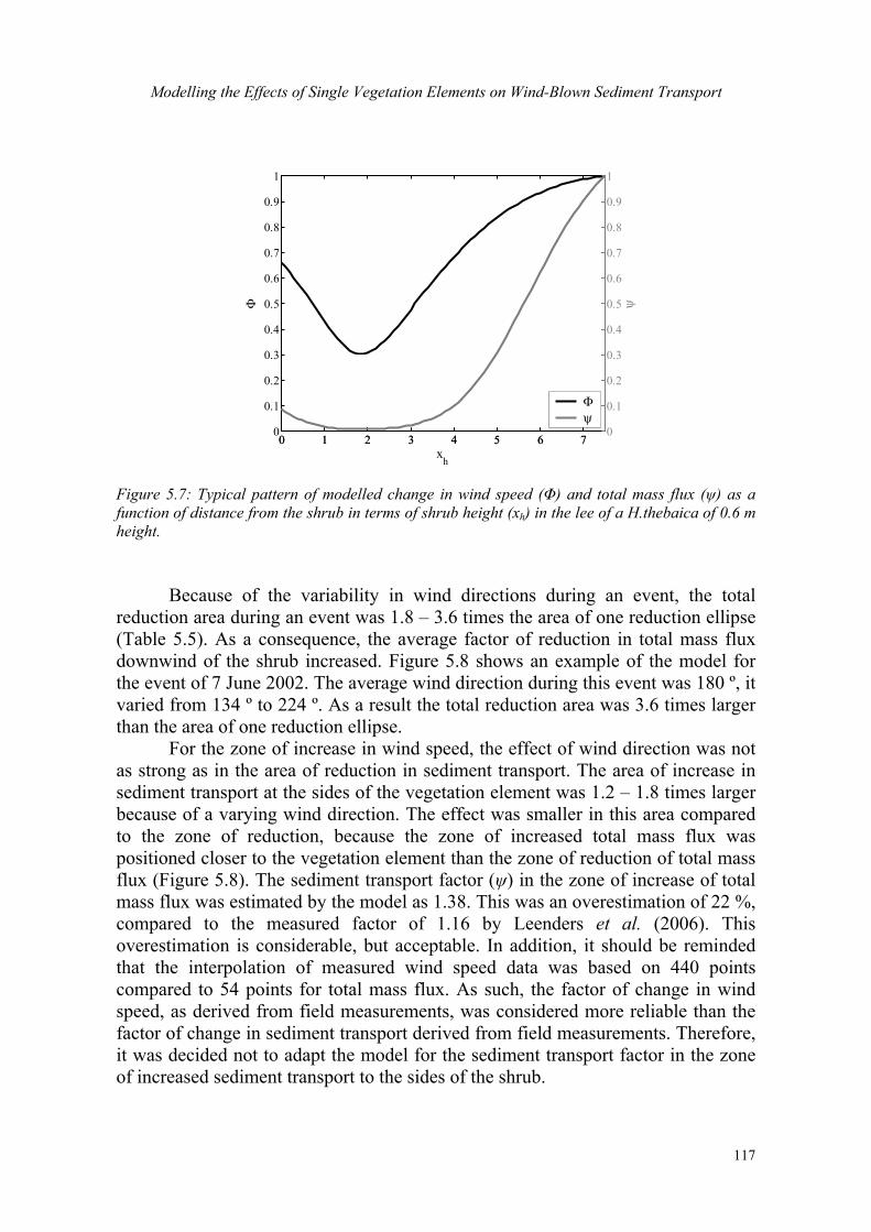
Modelling the Effects of Single Vegetation Elements on Wind-Blown Sediment Transport
117
0 1 2 3 4 5 6 70
0.1
0.2
0.3
0.4
0.5
0.6
0.7
0.8
0.9
1
Φ
xh
Φψ
0 1 2 3 4 5 6 70
0.1
0.2
0.3
0.4
0.5
0.6
0.7
0.8
0.9
1
ψ
Figure 5.7: Typical pattern of modelled change in wind speed (Φ) and total mass flux (ψ) as a function of distance from the shrub in terms of shrub height (xh) in the lee of a H.thebaica of 0.6 m height.
Because of the variability in wind directions during an event, the total
reduction area during an event was 1.8 – 3.6 times the area of one reduction ellipse (Table 5.5). As a consequence, the average factor of reduction in total mass flux downwind of the shrub increased. Figure 5.8 shows an example of the model for the event of 7 June 2002. The average wind direction during this event was 180 º, it varied from 134 º to 224 º. As a result the total reduction area was 3.6 times larger than the area of one reduction ellipse.
For the zone of increase in wind speed, the effect of wind direction was not as strong as in the area of reduction in sediment transport. The area of increase in sediment transport at the sides of the vegetation element was 1.2 – 1.8 times larger because of a varying wind direction. The effect was smaller in this area compared to the zone of reduction, because the zone of increased total mass flux was positioned closer to the vegetation element than the zone of reduction of total mass flux (Figure 5.8). The sediment transport factor (ψ) in the zone of increase of total mass flux was estimated by the model as 1.38. This was an overestimation of 22 %, compared to the measured factor of 1.16 by Leenders et al. (2006). This overestimation is considerable, but acceptable. In addition, it should be reminded that the interpolation of measured wind speed data was based on 440 points compared to 54 points for total mass flux. As such, the factor of change in wind speed, as derived from field measurements, was considered more reliable than the factor of change in sediment transport derived from field measurements. Therefore, it was decided not to adapt the model for the sediment transport factor in the zone of increased sediment transport to the sides of the shrub.
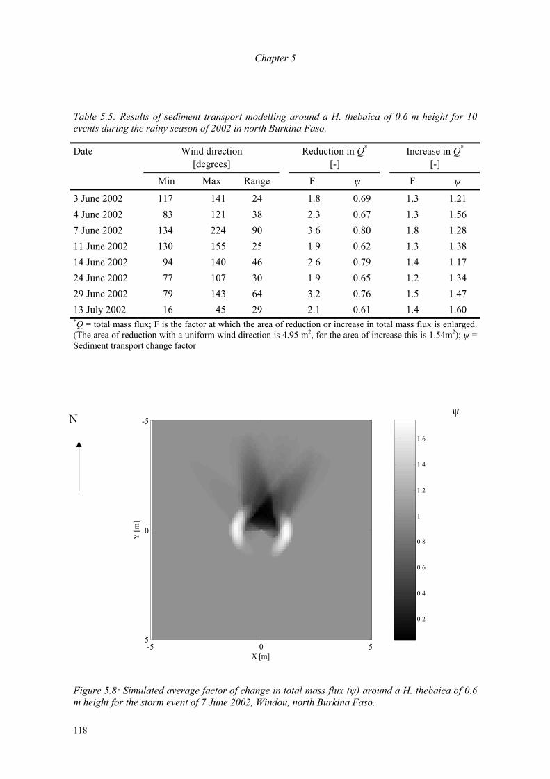
Chapter 5
118
Table 5.5: Results of sediment transport modelling around a H. thebaica of 0.6 m height for 10 events during the rainy season of 2002 in north Burkina Faso.
Date
Wind direction [degrees]
Reduction in Q*
[-] Increase in Q*
[-]
Min Max Range F ψ F ψ
3 June 2002 117 141 24 1.8 0.69 1.3 1.21 4 June 2002 83 121 38 2.3 0.67 1.3 1.56 7 June 2002 134 224 90 3.6 0.80 1.8 1.28 11 June 2002 130 155 25 1.9 0.62 1.3 1.38 14 June 2002 94 140 46 2.6 0.79 1.4 1.17 24 June 2002 77 107 30 1.9 0.65 1.2 1.34 29 June 2002 79 143 64 3.2 0.76 1.5 1.47 13 July 2002 16 45 29 2.1 0.61 1.4 1.60 *Q = total mass flux; F is the factor at which the area of reduction or increase in total mass flux is enlarged. (The area of reduction with a uniform wind direction is 4.95 m2, for the area of increase this is 1.54m2); ψ = Sediment transport change factor
0.2
0.4
0.6
0.8
1
1.2
1.4
1.6
X [m]
Y [m
]
-5 0 5
-5
0
5
Figure 5.8: Simulated average factor of change in total mass flux (ψ) around a H. thebaica of 0.6 m height for the storm event of 7 June 2002, Windou, north Burkina Faso.
ψ N
Modelling the Effects of Single Vegetation Elements on Wind-Blown Sediment Transport
119
5.5 Discussion and Conclusion This study showed that sediment transport was predicted best with a simple empirical equation of Radok (1977). It expresses the total mass flux being exponential to the wind velocity and two empirical constants. One of the empirical constants t was the ”growth” factor of sediment transport and could be fixed at 0.7 s m-1 for each storm. The other empirical constant can be interpreted as the erodibility of the soil. But the variability of events in this study was so diverse that this ‘erodibility’ parameter could not be fixed. It showed an increasing trend during the growing season. The analysis of this study raises the question as to whether a general transport model exists, knowing that field conditions are variable, both in space and time. It was concluded that in order to predict sediment transport adequately, modelling results should always be supported and substantiated by actual measurements of sediment transport and/or an accurate documentary on the soil erodibility factors.
A model was developed to simulate wind speed and sediment transport around a single shrub-type vegetation element. In this model, porosity, height and width of the vegetation element determine the extent of the wake zone. Porosity mainly determines the position of minimum wind speed and the rate of recovery of wind speed – the less porous the obstacle, the more effective the protection. A curve describing wind speed changes in the lee of a shrub with a porosity of only 18 % was tested for a shrub with a porosity of 79 % and agreed reasonably well with measured data. The estimation of wind speed along the centre line in the lee of the shrub up to 7.5 times the element height was acceptable. But, it should be mentioned that very dense obstacles can induce an area of recirculating eddies in the immediate lee, with increased turbulence (Cleugh, 1998). For such obstacles the wind changes show a lower minimum wind speed, because the rate of wind speed recovery is faster near the lee of the obstacle and slower thereafter. Low porosity obstacles are assumed to be less effective in reducing wind velocity than medium porosity obstacles (Wang and Takle, 1996). Cornelis and Gabriels (2005) concluded that a porosity of 20 - 35 % is optimal for wind barriers in terms of wind-velocity reduction. Ruck and Schmitt (1986) who used Laser-Doppler-Anemometry in a wind tunnel, also showed that porosity, height and width of an obstacle determine the extent of a wake zone. They also found that airflow around a vegetation element with a trunk differed from that without, due to the flow underneath the canopy. This difference was noticed immediately downwind of the obstacle as well as further downwind. Leenders et al. (2006) illustrated this difference in morphology among vegetation elements with respect to the airflow pattern from experimental results in a farmer’s field.
Gross (1987) developed a numerical model for the airflow around individual trees, both with and without a trunk. His results corresponded qualitatively well with the wind tunnel measurements of Ruck and Schmitt (1986). The model of Gross (1987) is merely physically based; it uses the Navier Stokes equations, the
Chapter 5
120
continuity equation and the first law of thermodynamics. The model presented here is empirically based and is a relatively simple model and therefore easy to apply by researchers, extension workers and others who aim to develop wind erosion control strategies that use scattered vegetation. It only simulates wind flow and sediment transport around shrubs. Currently it can not be used to simulate sediment transport near trees.
For the shrub tested in this study, a reduction of 57 % in total mass flux was simulated in its lee. To the sides an increase of 38 % in total mass flux was simulated. As the area of the zone of reduction in total mass flux was larger than the area of the zone of increase in total mass flux, the model simulated a net reduction in total mass flux around a shrub, as was observed in field measurements (Leenders et al., 2006). In addition, during a storm event with variable wind directions, the area over which a shrub affects total mass flux increased. These findings suggest that shrubs, being scattered in a farmer’s field could be used as a tool to diminish and control sediment transport, and thus wind erosion in a field.
But, in order to develop a control strategy that uses shrubs or scattered woody vegetation to control sediment transport, it is necessary to understand the effects of scattered vegetation on a larger scale than a single vegetation element, i.e. the scale of a field or several fields. These effects comprise the arrangement of vegetation elements together with the distribution in type, height, width and porosity of vegetation elements, the interaction between vegetation elements and their effects to extract momentum form the air at a larger scale (Gross, 1987; Wolfe and Nickling, 1993; Musick et al., 1996). The model presented in this paper is not yet adequate to describe these conditions and therefore should be further developed to include the effects of trees on wind speed and sediment transport. If scaled up effectively, the model could be used to determine the effect of different vegetation patterns with different vegetation characteristics. The results could subsequently be used to develop wind erosion control strategies by using scattered vegetation.
Modelling the Effects of Single Vegetation Elements on Wind-Blown Sediment Transport
121
References Alfaro S.C., Rajot J.L., Nickling W. 2004: Estimation of PM20 emissions by wind erosion: main
sources of uncertainties. Geomorphology 59: 63-74. Bagnold R.A. 1941: The physics of blown sand and desert dunes. Methuen. London. 265 pp. Bielders C.L., Alvey S., Cronyn N. 2001: Wind erosion: The perspective of grass-roots
communities in the Sahel. Land Degradation & Development 12: 57 - 70. Camp D.W., Turner R.E., Gilchris L.P. 1970: Response tests of cup, vane and propeller wind
sensors. Journal of Geophysical Research 75: 5265-5270. Chepil W.S. 1956: Influence of moisture on erodibility of soil by wind. Soil Science Society of
America Journal 20: 288-292. Cleugh H.A. 1998: Effects of windbreaks on airflow, microclimates and crop yields. Agroforestry
Systems 41: 55 - 84. Cornelis W.M., Gabriels D. 2005: Optimal windbreak design for wind erosion control. Journal of
Arid Environments 61: 315-332. Cornelis W.M., Oltenfreiter G., Gabriels D., Hartman R. 2004: Splash-Saltation of sand dune to
wind-driven rain: Horizontal flux and sediment transport rate. Soil Science Society of America Journal 68: 41-46.
Dong Z., Liu X., Wang H., Wang X. 2003: Aeolian sand transport: a wind tunnel model. Sedimentary Geology 161: 71-83.
Fryrear D.W. 1985: Soil cover and wind erosion. Transactions of the ASAE 28: 781-784. Fryrear D.W., Krammes C.A., Williamson D.L., Zobeck T.M. 1994: Computing the wind erodible
fraction of soils. Journal of Soil and Water Conservation 49: 183-188. Goossens D. 2000: Wind tunnel and field calibration of five aeolian sand traps. Geomorphology
35: 233-252. Goossens D. 2004: Effect of soil crusting on the emission and transport of wind-eroded sediment:
field measurements on loamy sandy soil. Geomorphology 58: 145-160. Grant P.F., Nickling W.G. 1998: Direct field measurement of wind drag on vegetation for
application to windbreak design and modelling. Land Degradation and Development 9: 57-66.
Greely R., Iversen J.D. 1985: Wind as a Geological Process. Cambridge University Press. 333 pp. Gross G. 1987: A numerical study of the air flow within and around a single tree. Boundary-Layer
Meteorology 40: 311-327. Hagen L.J. 1998: WEPS: Wind Erosion Prediction System. Iversen J.D., Rasmussen K.R. 1999: The effect of wind speed and bed slope on sand transport.
Sedimentology 46: 723-731. Kenney W.A. 1987: A Method for estimating windbreak porosity using digitized photographic
silhouettes. Agricultural and Forest Meteorology 39: 91-94. Kuhlman H. 1958: Quantitative measurements of aeolian sand transport. Geografisk Tidsskrift 57. Leenders J.K., Visser S.M., Stroosnijder L. 2005a: Farmers' perceptions of the role of scattered
vegetation in wind erosion control in Burkina Faso. Land Degradation & Development 16: 327-337.
Leenders J.K., van Boxel J.H., Sterk G. 2005b: Wind forces and related saltation transport. Geomorphology 71: 357-372.
Leenders J.K., van Boxel J.H., Sterk G. 2006: The effect of single vegetation elements on wind speed and sediment transport in the Sahelian zone of Burkina Faso. Accepted for publication in: Earth Surface Processes and Landforms.
McKenna Neuman C. 1998: Particle transport and adjustments of the boundary layer over rough surfaces with an unrestricted, upwind supply of sediment. Geomorphology 25: 1-17.
Michels K., Sivakumar M.V.K., Allison B.E. 1995: Wind erosion control using crop residue I. Effects on soil flux and soil properties. Field Crops Research 40: 101-110.

Modelling the Effects of Single Vegetation Elements on Wind-Blown Sediment Transport
123
Sterk G., Stein A., Stroosnijder L. 2004: Wind effects on spatial variability in pearl millet yields in the Sahel. Soil &Tillage Reseachr 76: 25 - 37.
Stout J.E., Zobeck T.M. 1996: Establishing the threshold condition for soil movement in wind-eroding fields. pp 65-71. In: Proceedings of the International Conference on air pollution from agricultural operations MidWest Plan Service (MWPS C-3), Kansas City.
Taylor-Powell E. 1991: Integrated management of agricultural watersheds: Land tenure and indigenous knowledge of soil and crop management. T. S. B. 91-04 Texas A&M University: College Station. TX, USA.
Van de Ven T.A.M., Fryrear D.W., Spaan W.P. 1989: Vegetation characteristics and soil loss by wind. Journal of Soil and Water Conservation 44: 347-349.
Visser S.M., Sterk G., Snepvangers J.J.J.C. 2004: Spatial variation in wind-blown sediment transport in geomorphic units in northern Burkina Faso using geostatical mapping. Geoderma 120: 95-107.
Wang H., Takle E.S. 1996: Momentum budget and shelter mechanism of boundary-layer flow near a shelterbelt. Boundary Layer Meteorology 82: 417-435.
Wolfe S.A., Nickling W.G. 1993: The protective role of sparse vegetation in wind erosion. Progress in Physical Geography 17: 50-68.
Zingg A.W. 1953: Wind-tunnel studies of the movement of sedimentary material. pp 111-135. In: Proceedings of the 5th Hydraulic Conference, Iowa City. Institute of Hydraulics.
Chapter 5
122
Mohammed A.E., Stigter C.J., Adam H.S. 1995: Moving sand and its consequences on and near a severely desertified environment and a protective shelterbelt. Arid soil Research and Rehabilitation 9: 423-435.
Musick H.B., Trujillo S.M., Truman C.R. 1996: Wind-tunnel modelling of the influence of vegetation structure on saltation threshold. Earth Surface Processes and Landforms 21: 589-605.
Namikas S.L., Sherman D.J. 1995: A review of the effects of surface moisture content on aeolian sand transport. pp 269 - 293. In: V. P. Tchakerian Ed. Desert Aeolian Processes. Chapman and Hall, London.
Namikas S.L., Bauer B.O., Sherman D.J. 2003: Influence of averaging interval on shear velocity estimates for aeolian transport modeling. Geomorphology 53: 235 - 246.
O'Brien M.P., Rindlaub B.D. 1936: The transportation of sand by wind. Civil Engineering 6: 325-327.
Radok U. 1977: Snow drift. Journal of Glaciology 19: 123-139. Raupach M.R., Thom A.S., Edwards I. 1980: A wind-tunnel study of turbulent flow close to
regularly arrayed rough surfaces. Boundary-Layer Meteorology 18: 373-397. Raupach M.R., Woods N., Dorr G., Leys J.F., Cluegh H.A. 2001: The entrapment of particles by
windbreaks. Atmospheric Environment 35: 3373 - 3383. Rice M.A., McEwan I.K. 2001: Crust strength: A wind tunnel study of the effect of impact by
saltating particles on cohesive soil surfaces. Earth Surface Processes and Landforms 26. Rinaudo T. 1996: Tailoring wind erosion control methods to farmers' specific needs. pp 161-171.
In: v. M. Oppen. Proceedings of the International Symposium on 'Wind Erosion in West Africa: The Problem and its Control', Hohenheim, Germany, 5-7 December 1994. Margraf Verlag, Weikersheim, Germany.
Ruck V.B., Schmitt F. 1986: Das Strömungsfeld der Einzelbaumuströmung. Abschätzung von Depositionswahrscheinlichkeiten für Feinsttröpfchen. Forstwissenschaftliches Centralblatt 105: 178 - 196.
Schönfeldt H.J., Von Löwis S. 2003: Turbulence-driven saltation in the atmospheric surface layer. Meteorologische Zeitschrift 12: 257-268.
Shao Y. 2000: Physics and modelling of wind erosion. R. Sadourny Atmospheric and Oceanographic Sciences Library, Vol. 23, Kluwer Academic Publishers. Dordrecht. 393 pp pp.
Sherman D.J., Jackson D.W.T., Namikas S.L., Wang J. 1998: Wind-blown sand on beaches: an evaluation of models. Geomorphology 22: 113 - 133.
Spaan W.P., Van den Abeele G.D. 1991: Wind borne particle measurements with acoustic sensors. Soil Technology 4: 51-63.
Sterk G. 1993: Sahelian wind erosion research project, Report III. Description and calibration of sediment samplers. Dep. of Irrigation adn Soil & Water Conservation, Wageningen University. Wageningen, The Netherlands. pp.
Sterk G. 2003: Causes, consequences and control of wind erosion in Sahelian Africa: A review. Land Degradation & Development 14: 95 - 108.
Sterk G., Raats P.A.C., 1996: Comparison of models describing the vertical distribution of wind-eroded sediment. Soil Science Society of America Journal 60: 1914-1919.
Sterk G., Stein A. 1997: Mapping wind-blown mass transport by modeling variability in space and time. Soil Science Society of America Journal 61: 232-239.
Sterk G., Haigis J. 1998: Farmers' knowledge of wind erosion processes and control methods in Niger. Land Degradation & Development 9: 107 - 114.
Sterk G., Hermann L., Bationo A. 1996: Wind-blown nutrient transport and soil poductivity changes in southwest Niger. Land Degradation & Development 7: 325-335.
Sterk G., Jacobs A.F.G., van Boxel J.H. 1998: The effect of turbulent flow structures on saltation transport in the atmospheric boundary layer. Earth Surface Processes and Landforms 23: 877-887.

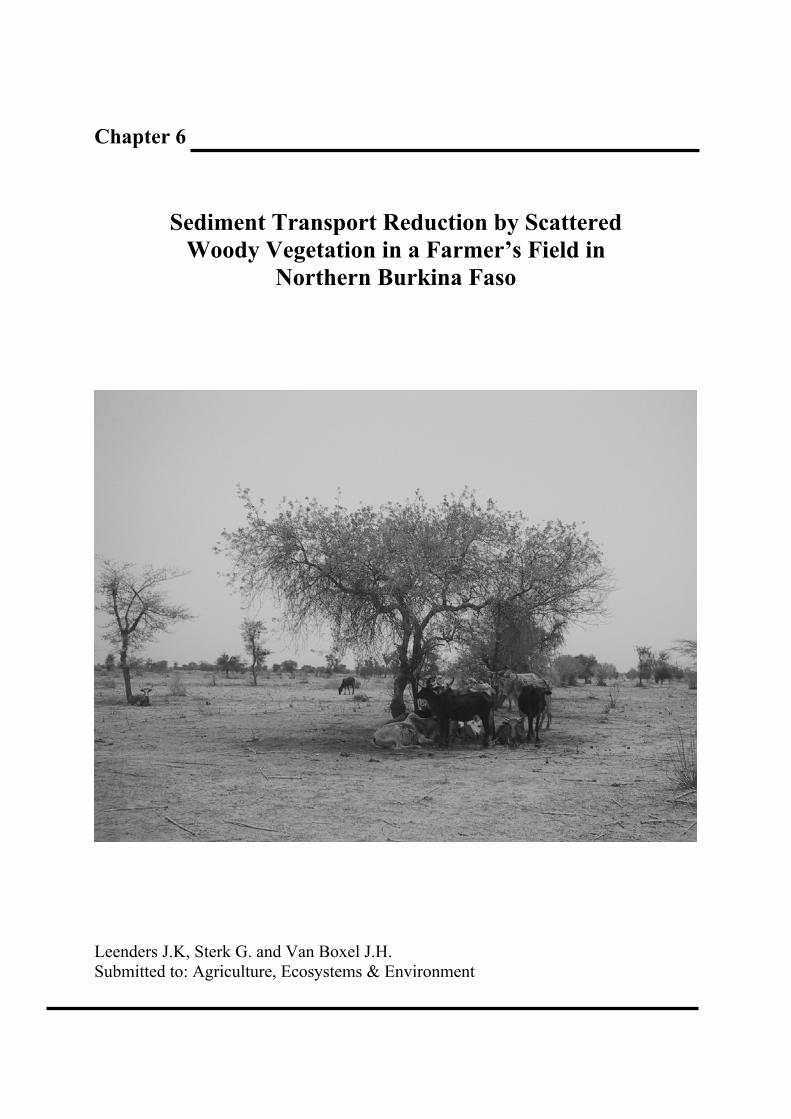
Chapter 6
Sediment Transport Reduction by Scattered Woody Vegetation in a Farmer’s Field in
Northern Burkina Faso
Leenders J.K, Sterk G. and Van Boxel J.H. Submitted to: Agriculture, Ecosystems & Environment

Chapter 6
128
are usually of short duration, 10 – 30 minutes in general, the soil movement that occurs during these events is much more intense than the soil movement during the ‘Harmattan’ (Michels et al., 1995).
By using control measures, wind erosion can be reduced. Wind erosion control measures either decrease the strength of the wind at the soil surface or increase the resistance of the soil surface, or both. However, at present, adoption of wind erosion control measures by Sahelian farmers is low (Sterk and Haigis, 1998; Bielders et al., 2001;Visser et al., 2003), as most recommended measures do not fit into the local farming systems (Baidu-Forson and Napier, 1998). For example despite the fact that the use of sand ridges, mulching and windbreaks, have been tested and proved to be effective in diminishing wind erosion in the Sahel (Mohammed et al., 1995; Michels et al., 1995; Sterk and Spaan, 1997; Bielders et al., 2000), these measures are not widely applied. This is partly attributed to certain disadvantages inherent to these measures. Sand ridges perpendicular to the prevailing wind are easily destroyed by rain (Bielders et al., 2000). In case of mulch, the availability of mulch material is limited (Michels et al., 1995) and the effect of a certain mulch cover decreases as the average wind speed of a storm increases (Sterk and Spaan, 1997; Sterk, 2000). Wind barriers are not widely applied, because they reduce crop growth due to competition for water, light and nutrients (Lamers et al., 1995). In addition, farmers also pointed out that some measures were not implemented because of lack of labour and resources, or because they were not familiar with certain measures (Visser et al., 2003). Thus there is a need for wind erosion control measures that actually fit in the local farming systems and do not require much additional input of labour and resources.
Studies carried out in Niger (Taylor-Powell, 1991; Rinaudo, 1996; Sterk and Haigis, 1998; Bielders et al., 2001), and in Burkina Faso (Leenders et al., 2005a) reported the farmers’ interest in reducing wind erosion through regeneration of the natural woody vegetation in cropland. Landscapes in which scattered vegetation of trees and shrubs occurs in cultivated or recently fallowed fields is called a ‘parkland system’ (Boffa, 1999). It is highly appreciated by farmers, because the by-products of the trees are a source of food, fodder, firewood, medicine and construction material (Petit, 2003). But, much of the standing natural woody vegetation in cropland has disappeared because of climatic change and human activity (Le Houérou, 1997). Development projects encourage farmers to regenerate the natural vegetation and some successes on regeneration of natural vegetation have been obtained in the south of Niger (Bielders et al., 2001; Yamba et al., 2005) and on the Central Plateau of Burkina Faso (Reij et al., 2005). In the south of Niger, natural regeneration of woody vegetation was actually used as a wind erosion control strategy (Rinaudo, 1996). The developed strategy was successful in reducing wind erosion and improving crop yields, but was developed from trial and error testing of different strategies. Given the site-specific conditions during its development it is uncertain whether this strategy can be transferred to other places, where environmental conditions are different.
Sediment Transport Reduction by Scattered Woody Vegetation in a Farmer’s Field
127
6 Sediment Transport Reduction by Scattered Woody
Vegetation in a Farmer’s Field in Northern Burkina Faso
Abstract This paper reports on an analysis on the effect of scattered vegetation on sediment transport in a farmers’ field in the north of Burkina Faso. For this purpose a model was adapted that was developed to simulate the alteration of wind speed and sediment transport around shrubs (single vegetation elements with low hanging braches). The performance of the developed model was verified by using field measurements on sediment transport that were obtained on two farmers’ fields in north Burkina Faso during the rainy season of 2003. The characteristics of the vegetation and the density of vegetation elements differed per field. The model was used to do scenario studies to test the effect of height, number, element type and spatial arrangement of vegetation elements on aeolian sediment transport. It was concluded that the performance of the model would possibly improve by including the aspects of topography and sediment availability. In addition it was recommended to test the model in a variety of sparsely vegetated terrains.
From the scenarios it appeared that the effects on wind speed and sediment transport in the vicinity of vegetation elements, although present, are small compared to the effects vegetation elements exert on sediment transport by influencing the aerodynamic roughness length. With relatively small changes in the characteristics of scattered woody vegetation, sediment transport could change considerable. Therefore it was concluded that scattered woody vegetation can be used to reduce sediment transport. Applying scattered woody vegetation to reduce sediment transport effectively, involves cooperation of farmers. Regeneration and management of vegetation at village level is advocated. The optimal arrangement of vegetation elements in an area is an interrelation between the number of vegetation elements, the silhouette area and the type of vegetation elements present. Based on this study it is concluded that the use of scattered vegetation as a wind erosion control strategy is an attractive and promising tool, it fits in a variety of farming systems and can easily be adapted to specific needs of farmers. 6.1 Introduction The Sahelian zone of Africa is the region that is globally most subjected to land degradation, with wind erosion being the most important soil degradation process (Valentin, 1995). Wind erosion occurs whenever the forces of the wind exceed the resistance of the soil. In the Sahel, wind erosion occurs mainly during two periods of the year: in the dry season (October – April) and in the early rainy season (May – July). During the dry season, the Sahel is invaded by the so-called ‘Harmattan’; dry and rather strong winds, that blow south-west and west off the Sahara. These winds mostly carry much dust and cause moderate wind erosion (Michels et al., 1995). The wind erosion that occurs at the start of the rainy season is caused by strong windstorms that precede convective rainstorms. Although these windstorms
Sediment Transport Reduction by Scattered Woody Vegetation in a Farmer’s Field
129
Using the parkland system as a wind erosion control strategy seems promising for several reasons: 1) the soil loss is expected to reduce because of the standing natural vegetation amongst the crop; 2) a negative effect on crop production, due to competition between trees, shrubs and crops for light, nutrients and water is limited, because of the scattered pattern of the woody vegetation; 3) the by-products of trees and shrubs can be useful for the farmer for different purposes; 4) the strategy doesn’t require additional management skills or tools of local people because it addresses knowledge on natural vegetation that is already present.
Before promoting the parkland system as a wind erosion control strategy, the effect of scattered woody vegetation on wind erosion should be understood and quantified. Data of measurements on wind speed and sediment transport around isolated vegetation elements showed that the morphology of elements determines the effects on wind speed and sediment transport (Ruck and Schmitt, 1986; Leenders et al., 2006a). Two types of elements can be distinguished; elements with a canopy starting at the soil surface and elements which have a distinctive trunk with a canopy above it. In this paper the first type of elements is referred to as ‘shrubs’ and the second type of elements as ‘trees’. Shrubs were found to reduce wind speed and sediment transport up to approximately 7.5 times the height of the element (Leenders et al., 2006a; 2006b). The extent of reduction in wind speed downward of a shrub depends mainly on the porosity of the element and the position downwind. In addition, material already in transport was trapped effectively by shrubs. Trees showed a different effect on wind speed and sediment transport. Below the canopy and around the trunk, streamlines are contracted resulting in an increased wind speed and sediment transport. In addition to these local effects, the presence of trees and shrubs has also an effect at the larger scale. Both trees and shrubs extract momentum from the wind, which diminishes the wind speed in an area. As trees are generally larger in height and width than shrubs, it is expected that trees are more effective in reducing the wind speed in an area than shrubs (Leenders et al., 2006a).
The degree of erosion protection by different vegetation elements and the optimal vegetation arrangement to protect Sahelian cropland from wind erosion is currently unknown. The aim of this study was to determine the impact of scattered woody vegetation on sediment transport in a farmers’ field in the north of Burkina Faso. First a model was developed to simulate sediment transport influenced by vegetation elements in a field. Then, this model was used to determine 1) the effect of height and number of vegetation elements on sediment transport; 2) the effect of the distribution of element types on sediment transport (i.e. ratio of number of trees and shrubs); and 3) the effect of spatial arrangement of vegetation elements on sediment transport.
Chapter 6
130
6.2 Materials and Methods 6.2.1 Study area During the rainy season of 2003, experimental work was carried out in two agricultural fields, located at approximately 7 km (field B) and 12 km (field A) east of Dori in north Burkina Faso. The area is part of the southern Sahelian zone, which is characterized by high temperatures all year round and a short rainy season of 4 months, from June to September. The average annual rainfall is 420 mm, but variability in annual rainfall is high. For example, during the rainy season of 2003 the total amount of rainfall was 1050 mm.
The soil texture in the experimental fields was loamy sand. Field A had 82.1 % sand, 13.6 % silt and 4.3 % clay in the topsoil (0-5 cm), with a median particle size of 134 µm, and field B had 85.5 % sand, 11.1 % silt and 3.4 % clay in the topsoil, with a median particle size of 141 µm. The main crop in both experimental fields was pearl millet (Pennisetum glaucum), intercropped with cowpea (Vigna unguiculata). Within both fields, natural vegetation was present. The most common vegetation species were Acacia raddiana, Maeura crassifolia and Balanites aegyptiaca in field A, and Piliostigma reticulatum, Faidherbia albida, Balanites aegyptiaca, Sclerocary birrea and Ziziphus mauritiana in field B. 6.2.2 Field measurements On both fields a detailed vegetation survey was carried out in a plot of 100 x 100 m. Within this plot the vegetation species were determined, and characteristics of the vegetation that influence wind speed and sediment transport were measured. These characteristics were trunk height and trunk width (for trees only), total height, canopy width (both in NS and EW directions), the location in the plot, and optical porosity of the canopy. The latter was estimated using digital pictures and image software, similar to the method of Kenney (1987). The species, height and width of the vegetation in the rest of the experimental fields were also determined.
Wind speed on both fields was measured with four cup-anemometers that were mounted on a mast at 0.75 m 1.25 m 2.25 m and 3.25 m at both fields. Every 5 seconds wind speed was sampled, and the average value was registered every minute. Wind direction was measured at 2.25 m with a wind vane at one-minute intervals. In addition a tipping bucket rain gauge was used to measure rainfall, every minute. The data were used to determine the duration of a windstorm prior to rainfall.
Sediment transport was measured with two saltiphones (Spaan and Van den Abeele, 1991), which is a robust sensor that counts impacts of saltating particles with a microphone. It can be used for detecting periods and intensities of saltation transport, but cannot be used to quantify the mass of particle flux (Goossens et al., 2000). The two saltiphones were placed 3 m in NE and SW directions of the meteorology mast, and the centre of the microphones was positioned at 0.10 m above the surface. The total mass of particle flux was measured with 17 MWAC
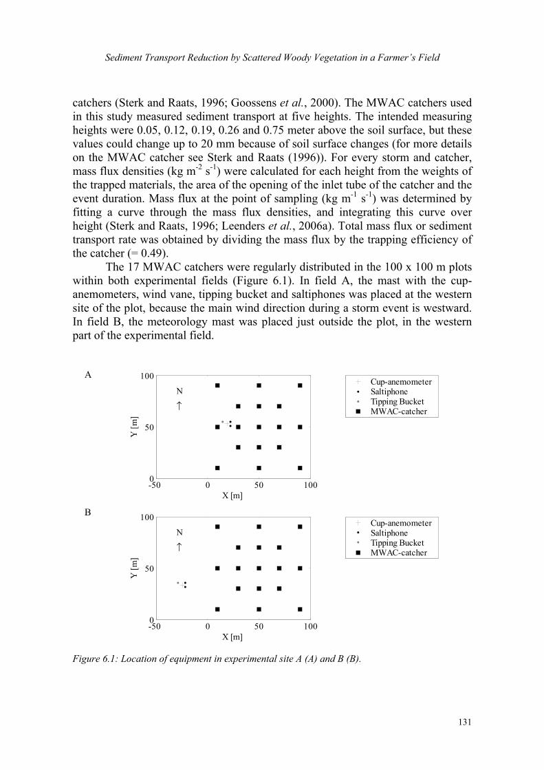
Sediment Transport Reduction by Scattered Woody Vegetation in a Farmer’s Field
131
catchers (Sterk and Raats, 1996; Goossens et al., 2000). The MWAC catchers used in this study measured sediment transport at five heights. The intended measuring heights were 0.05, 0.12, 0.19, 0.26 and 0.75 meter above the soil surface, but these values could change up to 20 mm because of soil surface changes (for more details on the MWAC catcher see Sterk and Raats (1996)). For every storm and catcher, mass flux densities (kg m-2 s-1) were calculated for each height from the weights of the trapped materials, the area of the opening of the inlet tube of the catcher and the event duration. Mass flux at the point of sampling (kg m-1 s-1) was determined by fitting a curve through the mass flux densities, and integrating this curve over height (Sterk and Raats, 1996; Leenders et al., 2006a). Total mass flux or sediment transport rate was obtained by dividing the mass flux by the trapping efficiency of the catcher (= 0.49).
The 17 MWAC catchers were regularly distributed in the 100 x 100 m plots within both experimental fields (Figure 6.1). In field A, the mast with the cup-anemometers, wind vane, tipping bucket and saltiphones was placed at the western site of the plot, because the main wind direction during a storm event is westward. In field B, the meteorology mast was placed just outside the plot, in the western part of the experimental field.
-50 0 50 1000
50
100
↑
N
X [m]
Y [m
]
Cup-anemometerSaltiphoneTipping BucketMWAC-catcher
-50 0 50 1000
50
100
↑
N
X [m]
Y [m
]
Cup-anemometerSaltiphoneTipping BucketMWAC-catcher
A
B
Figure 6.1: Location of equipment in experimental site A (A) and B (B).
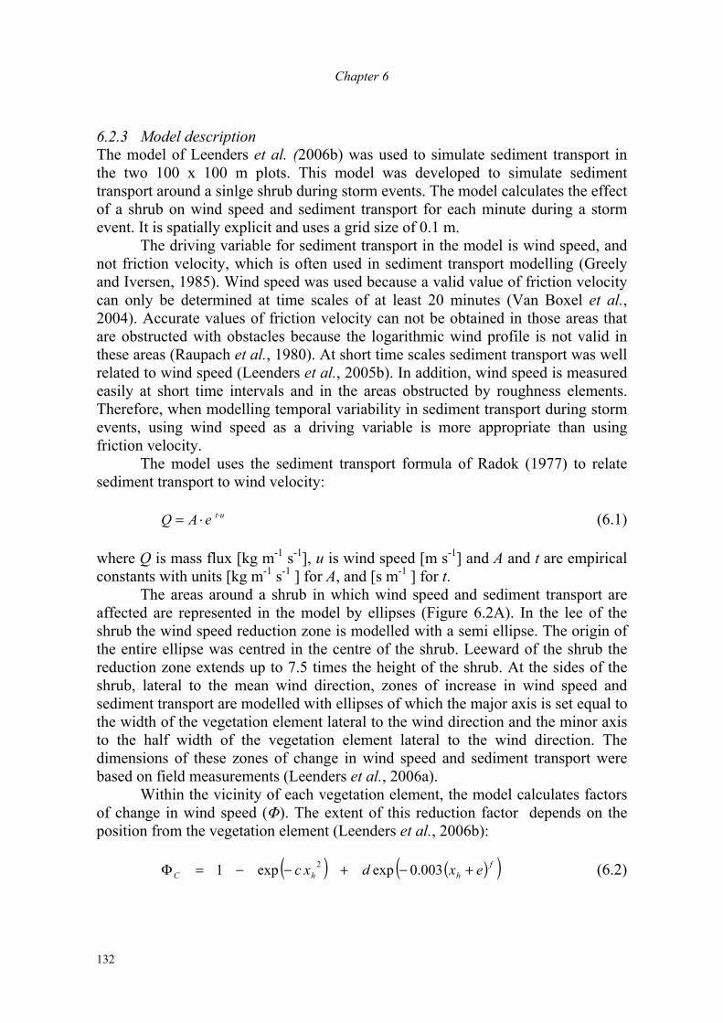
Chapter 6
132
6.2.3 Model description The model of Leenders et al. (2006b) was used to simulate sediment transport in the two 100 x 100 m plots. This model was developed to simulate sediment transport around a sinlge shrub during storm events. The model calculates the effect of a shrub on wind speed and sediment transport for each minute during a storm event. It is spatially explicit and uses a grid size of 0.1 m.
The driving variable for sediment transport in the model is wind speed, and not friction velocity, which is often used in sediment transport modelling (Greely and Iversen, 1985). Wind speed was used because a valid value of friction velocity can only be determined at time scales of at least 20 minutes (Van Boxel et al., 2004). Accurate values of friction velocity can not be obtained in those areas that are obstructed with obstacles because the logarithmic wind profile is not valid in these areas (Raupach et al., 1980). At short time scales sediment transport was well related to wind speed (Leenders et al., 2005b). In addition, wind speed is measured easily at short time intervals and in the areas obstructed by roughness elements. Therefore, when modelling temporal variability in sediment transport during storm events, using wind speed as a driving variable is more appropriate than using friction velocity.
The model uses the sediment transport formula of Radok (1977) to relate sediment transport to wind velocity:
uteAQ ⋅⋅= (6.1)
where Q is mass flux [kg m-1 s-1], u is wind speed [m s-1] and A and t are empirical constants with units [kg m-1 s-1 ] for A, and [s m-1 ] for t.
The areas around a shrub in which wind speed and sediment transport are affected are represented in the model by ellipses (Figure 6.2A). In the lee of the shrub the wind speed reduction zone is modelled with a semi ellipse. The origin of the entire ellipse was centred in the centre of the shrub. Leeward of the shrub the reduction zone extends up to 7.5 times the height of the shrub. At the sides of the shrub, lateral to the mean wind direction, zones of increase in wind speed and sediment transport are modelled with ellipses of which the major axis is set equal to the width of the vegetation element lateral to the wind direction and the minor axis to the half width of the vegetation element lateral to the wind direction. The dimensions of these zones of change in wind speed and sediment transport were based on field measurements (Leenders et al., 2006a).
Within the vicinity of each vegetation element, the model calculates factors of change in wind speed (Φ). The extent of this reduction factor depends on the position from the vegetation element (Leenders et al., 2006b):
( ) ( )( )f
hhC exdxc +−+−−=Φ 003.0expexp1 2 (6.2)

Sediment Transport Reduction by Scattered Woody Vegetation in a Farmer’s Field
133
where ΦC is the factor of change in wind speed along the centre line and xh is the distance downwind from the obstacle along the wind direction in terms of obstacle height. Equation 6.2 is based on the equation for wind speed reduction behind windbreaks developed by Hagen (1998). Coefficients c, d, e and f depend on the canopy porosity (θ):
)17.017.0008.0(13 05.1θθ +−=c (6.3)
( )2.05.0exp05.1 θ−=d (6.4)
( )θ5.015.2 −=e (6.5)
θ−= 5f (6.6) Off the centre line, the factors in reduction of wind speed were modelled
proportional to those on the centre line. The factor of change in wind speed at every location in the lee of the shrub was obtained by multiplying ΦC with a proportionality factor (ε ):
2
5.01 ⎟
⎠⎞
⎜⎝⎛−= wyε (6.7)
where yw is the y-coordinate of the ellipse, normalized with the width of the shrub. As such the reduction of wind speed in the lee of the shrub was represented in ellipses and sub-ellipses. (Figure 6.2B)
On both sides of the shrub, zones of increase in wind speed were modelled by using ellipses with a length equal to the width of the vegetation element and a width of half the width of the vegetation element (Figure 6.2C). In these zones wind speed was modelled with a simple quadratic curve:
12.125.05.0
12.0
222
+⎟⎟
⎠
⎞
⎜⎜
⎝
⎛
⎟⎟⎠
⎞⎜⎜⎝
⎛+⎟
⎟⎠
⎞⎜⎜⎝
⎛−=Φ
yy wy
wx (6.8)
where Φ is the factor of change in wind speed; x the coordinate of the increase ellipse along the wind direction, y the coordinate of the increase ellipse lateral to the wind direction; and wy the width of the vegetation element lateral to the wind direction. The coefficients of 0.5 and 0.25 within the parentheses form the boundaries of the increase ellipse. The coefficients -0.12 and 1.12 result in an average Φ of 1.06, which was measured in the field around a number of shrubs (Leenders et al., 2006a).
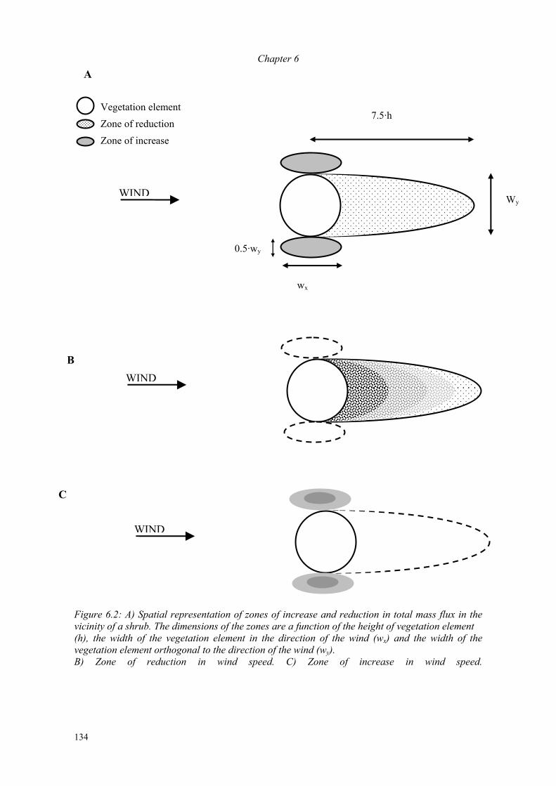
Chapter 6
134
Figure 6.2: A) Spatial representation of zones of increase and reduction in total mass flux in the vicinity of a shrub. The dimensions of the zones are a function of the height of vegetation element (h), the width of the vegetation element in the direction of the wind (wx) and the width of the vegetation element orthogonal to the direction of the wind (wy). B) Zone of reduction in wind speed. C) Zone of increase in wind speed.
WIND
WIND
wx
Wy
7.5·h
0.5·wy
WIND
A
B
C
Vegetation element Zone of reduction Zone of increase
Sediment Transport Reduction by Scattered Woody Vegetation in a Farmer’s Field
135
For each time step in the model, the central axis of the ellipses of reduction and increase in wind speed were oriented in the average wind direction for that time step. Each time step, a factor of change in wind speed (Φ) around the vegetation element was calculated. This factor was used to calculate an adapted wind speed around the shrub. With Radok’s transport equation (eq. 6.1), this adapted wind speed was converted to the sediment transport around the vegetation element. This sediment transport then was normalized with the sediment transport of unobstructed flow to calculate a sediment transport change factor (ψ). On the local scale, around an isolated shrub, the simulated change in sediment transport agreed reasonably well with the measured sediment transport (Leenders et al., 2006a).
In order to apply this model to simulate the effects of several vegetation elements in a field, the model needed to be adapted to include the following three aspects: 1) the local effects of tree-type vegetation elements (elements with a canopy above a trunk); 2) a parameterization to enable overlapping wake zones of vegetation elements; and 3) the effects of vegetation elements on the average wind speed in an area.
First, the extent of the local effect of increase in wind speed and sediment transport around the trunk of trees was included in the model (Figure 6.3). This extension was based on assumptions derived from field experiments (Leenders et al., 2006a). Windward, the wind speed was assumed to be affected up to 0.5 times the trunk height. Leeward this was set up to 5 times the trunk height. Sideward the influence was modelled to affect up to 2 times the diameter of the trunk (Figure 6.3).
Figure 6.3: Spatial representation of zone of increase in sediment transport in the vicinity of a tree. The dimensions of the zone are a function of the height (hT) and diameter of the trunk (dT). In this zone wind speed was modelled with a quadratic curve:
2.12
2.0
222
+⎟⎟
⎠
⎞
⎜⎜
⎝
⎛⎟⎟⎠
⎞⎜⎜⎝
⎛+⎟⎟
⎠
⎞⎜⎜⎝
⎛−=Φ
TT dy
hex (6.9)
Trunc Zone of increase
WIND 4 dT
5 hT 0.5 hT
Chapter 6
136
where Φ is the factor of change in wind speed; x the coordinate of the increase zone along the wind direction, y the coordinate of the increase zone lateral to the wind direction; hT the height of the trunk; dT the diameter of the trunk. The coefficient e was 0.5 windward and 5 leeward, indicating the boundaries of the zone of increase in wind speed in front of and behind the trunk. The coefficients -0.2 and 1.2 in equation 6.9 result in an average Φ of 1.1, which is in agreement with experimental derived values (Leenders et al., 2006a).
Second, the overlapping of zones of influence of several vegetation elements was included in the model by simply multiplying the wind speed factors (Φ) of the influence zones. Finally, the effects of vegetation elements on the larger scale were modelled by combining the exposure correction method of Wieringa (1976) with the simple aerodynamic roughness model of Lettau (1969). The method of Wieringa is based on the validity of the logarithmic wind profile in an area. It extrapolates the known wind speed profile in that area (area 1), to an area where aerodynamic roughness and shear stress are different because of different arrangement and characteristics of the roughness elements (area 2). From the measured wind profile in area 1, the wind speed is calculated at a height where wind speed is considered constant (e.g. 100 m), meaning that wind speed changes due to a different aerodynamic roughness at the surface are negligible. By estimating the aerodynamic roughness length z0 in area 2, and knowing the wind velocity near the surface in area 1, the wind velocity near the ground surface at area 2 can be calculated with:
)/100(ln
)/(ln)/(ln)/100(ln
)2(0
)2(0
)1(0
)1(012 z
zzzzz
UU ⋅⋅= (6.10)
Where U2 is the average wind speed in area 2 at station height z; U1 is the measured average wind speed in area 1 at station height z; z0(1) is the aerodynamic roughness length of area 1; and z0(2) is the aerodynamic roughness length at area 2. The change in aerodynamic roughness length (z0) was estimated with the simple model of Lettau (1969):
Sshz ⋅⋅= 5.0
0 (6.11)
where z0 is the aerodynamic roughness length [m], h is the average height of the vegetation element [m], s the silhouette area of the average obstacle [m2], and S is the specific area, or lot area [m2] measured in the horizontal plane, corrected for the number of vegetation elements (n). If n is the total number of roughness elements on a site of total area B, then nBS /= . The silhouette area of the average obstacle (s) is calculated by multiplying the average height of the obstacle ( h ) with the average width, lateral to the wind direction ( w ), corrected for the porosity of the
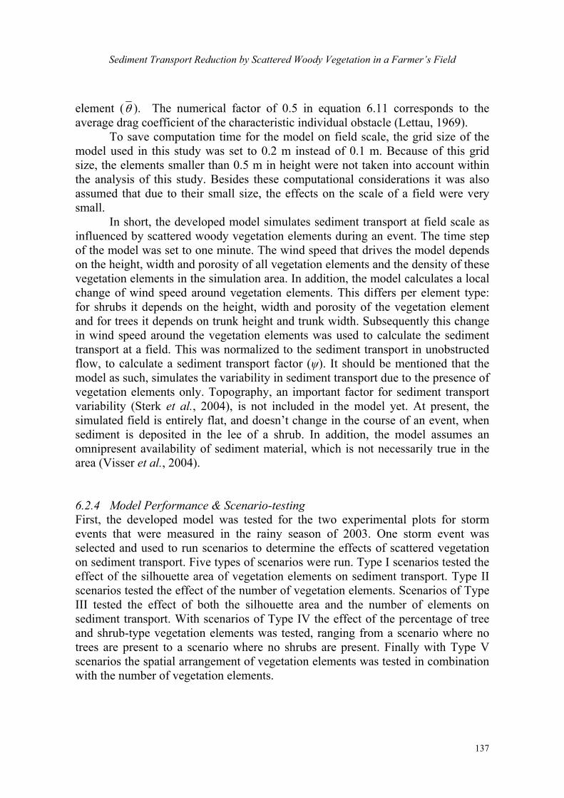
Sediment Transport Reduction by Scattered Woody Vegetation in a Farmer’s Field
137
element (θ ). The numerical factor of 0.5 in equation 6.11 corresponds to the average drag coefficient of the characteristic individual obstacle (Lettau, 1969).
To save computation time for the model on field scale, the grid size of the model used in this study was set to 0.2 m instead of 0.1 m. Because of this grid size, the elements smaller than 0.5 m in height were not taken into account within the analysis of this study. Besides these computational considerations it was also assumed that due to their small size, the effects on the scale of a field were very small.
In short, the developed model simulates sediment transport at field scale as influenced by scattered woody vegetation elements during an event. The time step of the model was set to one minute. The wind speed that drives the model depends on the height, width and porosity of all vegetation elements and the density of these vegetation elements in the simulation area. In addition, the model calculates a local change of wind speed around vegetation elements. This differs per element type: for shrubs it depends on the height, width and porosity of the vegetation element and for trees it depends on trunk height and trunk width. Subsequently this change in wind speed around the vegetation elements was used to calculate the sediment transport at a field. This was normalized to the sediment transport in unobstructed flow, to calculate a sediment transport factor (ψ). It should be mentioned that the model as such, simulates the variability in sediment transport due to the presence of vegetation elements only. Topography, an important factor for sediment transport variability (Sterk et al., 2004), is not included in the model yet. At present, the simulated field is entirely flat, and doesn’t change in the course of an event, when sediment is deposited in the lee of a shrub. In addition, the model assumes an omnipresent availability of sediment material, which is not necessarily true in the area (Visser et al., 2004).
6.2.4 Model Performance & Scenario-testing First, the developed model was tested for the two experimental plots for storm events that were measured in the rainy season of 2003. One storm event was selected and used to run scenarios to determine the effects of scattered vegetation on sediment transport. Five types of scenarios were run. Type I scenarios tested the effect of the silhouette area of vegetation elements on sediment transport. Type II scenarios tested the effect of the number of vegetation elements. Scenarios of Type III tested the effect of both the silhouette area and the number of elements on sediment transport. With scenarios of Type IV the effect of the percentage of tree and shrub-type vegetation elements was tested, ranging from a scenario where no trees are present to a scenario where no shrubs are present. Finally with Type V scenarios the spatial arrangement of vegetation elements was tested in combination with the number of vegetation elements.
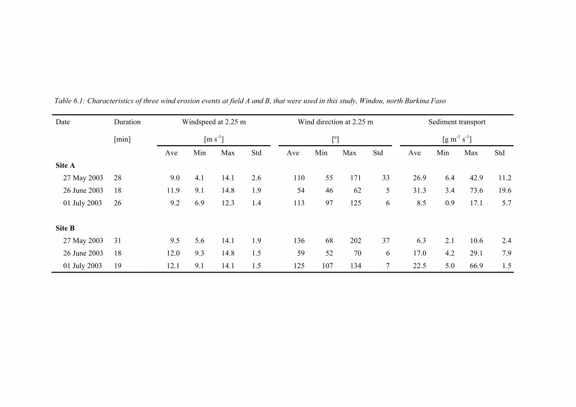
Table 6.1: Characteristics of three wind erosion events at field A and B, that were used in this study, Windou, north Burkina Faso Date Duration
[min]
Windspeed at 2.25 m
[m s-1]
Wind direction at 2.25 m
[º]
Sediment transport
[g m-1 s-1]
Ave Min Max Std Ave Min Max Std Ave Min Max Std
Site A
27 May 2003 28 9.0 4.1 14.1 2.6 110 55 171 33 26.9 6.4 42.9 11.2
26 June 2003 18 11.9 9.1 14.8 1.9 54 46 62 5 31.3 3.4 73.6 19.6
01 July 2003 26 9.2 6.9 12.3 1.4 113 97 125 6 8.5 0.9 17.1 5.7
Site B
27 May 2003 31 9.5 5.6 14.1 1.9 136 68 202 37 6.3 2.1 10.6 2.4
26 June 2003 18 12.0 9.3 14.8 1.5 59 52 70 6 17.0 4.2 29.1 7.9
01 July 2003 19 12.1 9.1 14.1 1.5 125 107 134 7 22.5 5.0 66.9 1.5
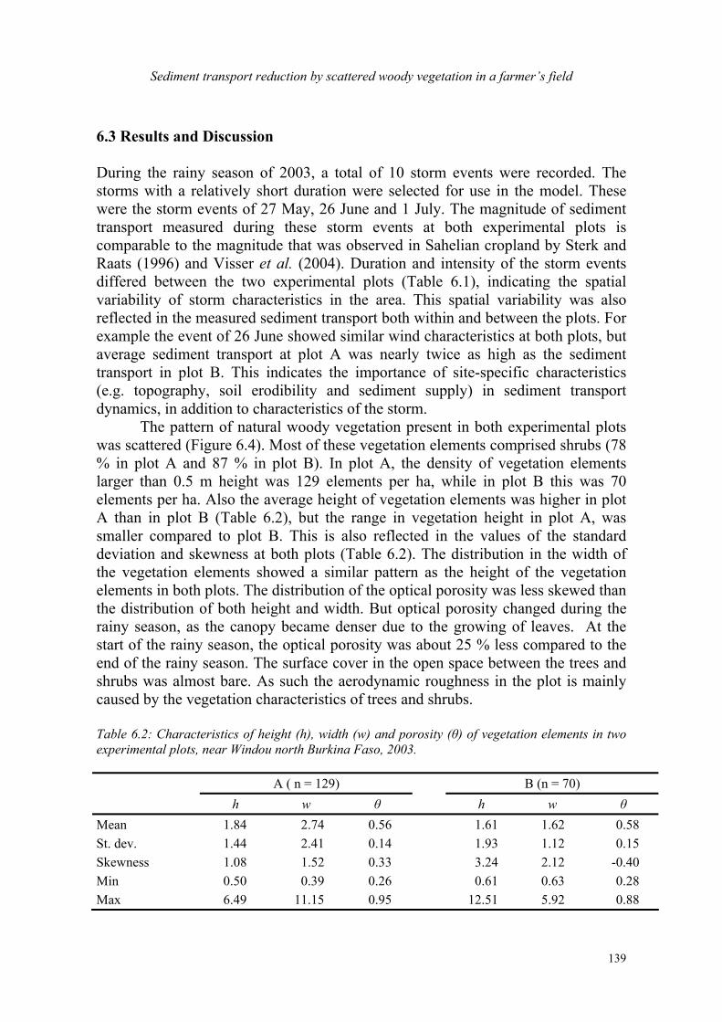
Sediment transport reduction by scattered woody vegetation in a farmer’s field
139
6.3 Results and Discussion During the rainy season of 2003, a total of 10 storm events were recorded. The storms with a relatively short duration were selected for use in the model. These were the storm events of 27 May, 26 June and 1 July. The magnitude of sediment transport measured during these storm events at both experimental plots is comparable to the magnitude that was observed in Sahelian cropland by Sterk and Raats (1996) and Visser et al. (2004). Duration and intensity of the storm events differed between the two experimental plots (Table 6.1), indicating the spatial variability of storm characteristics in the area. This spatial variability was also reflected in the measured sediment transport both within and between the plots. For example the event of 26 June showed similar wind characteristics at both plots, but average sediment transport at plot A was nearly twice as high as the sediment transport in plot B. This indicates the importance of site-specific characteristics (e.g. topography, soil erodibility and sediment supply) in sediment transport dynamics, in addition to characteristics of the storm.
The pattern of natural woody vegetation present in both experimental plots was scattered (Figure 6.4). Most of these vegetation elements comprised shrubs (78 % in plot A and 87 % in plot B). In plot A, the density of vegetation elements larger than 0.5 m height was 129 elements per ha, while in plot B this was 70 elements per ha. Also the average height of vegetation elements was higher in plot A than in plot B (Table 6.2), but the range in vegetation height in plot A, was smaller compared to plot B. This is also reflected in the values of the standard deviation and skewness at both plots (Table 6.2). The distribution in the width of the vegetation elements showed a similar pattern as the height of the vegetation elements in both plots. The distribution of the optical porosity was less skewed than the distribution of both height and width. But optical porosity changed during the rainy season, as the canopy became denser due to the growing of leaves. At the start of the rainy season, the optical porosity was about 25 % less compared to the end of the rainy season. The surface cover in the open space between the trees and shrubs was almost bare. As such the aerodynamic roughness in the plot is mainly caused by the vegetation characteristics of trees and shrubs. Table 6.2: Characteristics of height (h), width (w) and porosity (θ) of vegetation elements in two experimental plots, near Windou north Burkina Faso, 2003. A ( n = 129) B (n = 70) h w θ h w θ Mean 1.84 2.74 0.56 1.61 1.62 0.58 St. dev. 1.44 2.41 0.14 1.93 1.12 0.15 Skewness 1.08 1.52 0.33 3.24 2.12 -0.40 Min 0.50 0.39 0.26 0.61 0.63 0.28 Max 6.49 11.15 0.95 12.51 5.92 0.88
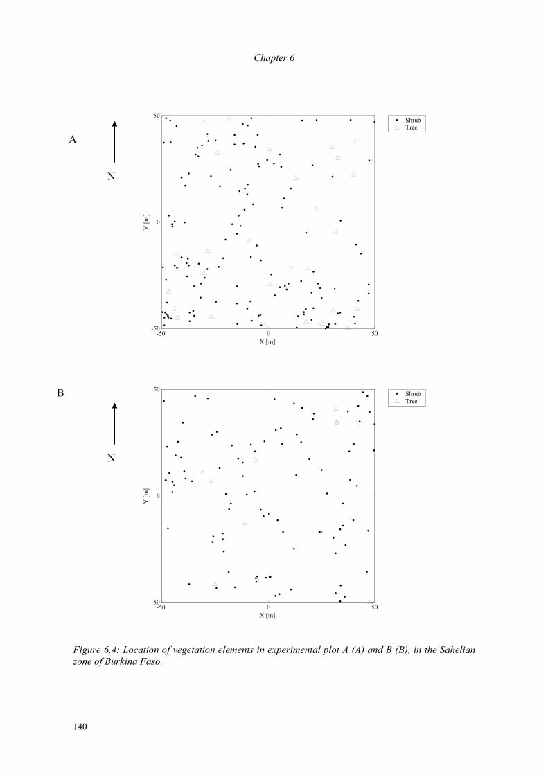
Chapter 6
140
-50 0 50-50
0
50
X [m]
Y [m
]
ShrubTree
-50 0 50-50
0
50
X [m]
Y [m
]
ShrubTree
Figure 6.4: Location of vegetation elements in experimental plot A (A) and B (B), in the Sahelian zone of Burkina Faso.
N
B
N
A
Sediment transport reduction by scattered woody vegetation in a farmer’s field
141
6.3.1 Estimation of Aerodynamic Roughness Length Lettau’s model (1969) predicted a value of z0 in plot A of 26 mm. In plot B this was 6 mm. The higher prediction in aerodynamic roughness length for plot A compared to plot B is mainly caused by the difference in density of vegetation elements. Overall, the estimated values of z0 are low. A z0-value of 6 mm corresponds to a roughness in a homogenous terrain of fallow ground, and a z0-value of 26 mm corresponds to values found in long grass and heather (Wieringa, 1993). The low values of z0 were attributed to the dispersed character of the vegetation and the bare surface in between the vegetation at the start of the growing season. The models of Lettau (1969) and Wieringa (1976) were applied to determine the effect of the present vegetation at both plots on wind speed compared to the situation when all woody vegetation would have been removed (bare plot). For this purpose the z0-value of a bare plot was taken as 0.5 mm. This z0-value corresponds to z0-values found in a flat desert (Wieringa, 1993). At a station height of 3.25 m at plot A, wind speed for a bare plot would have increased by 123 % compared to the current situation. For experimental plot B this was 111 %. Hence, the actual vegetation covers of woody vegetation in both plots had already a significant effect on the average wind speed.
In this study the model of Lettau was selected to model z0-values because of its simplicity and because it takes the effect of coverage, obstacle shape and height of the vegetation elements into account to calculate the z0-value. This was considered as an advantage over other simple models that estimate the value of z0 based on height alone (see Brutsaert, 1982). Wieringa (1993) stated that Lettau’s model is limited up to moderately inhomogeneous situations and its application in wake interference flow is not proven, but the results presented in Petersen (1997) extend the applicable range of the method to at least moderately inhomogeneous situations. According to Petersen (1997), Lettau’s model provides a good estimate of the surface roughness length. However, the research of Petersen (1997) comprised a wind tunnel study on industrial terrains, which differs from sparsely vegetated terrain. For the sparse vegetated surface of the Sahel Lettau’s model was applied by Lloyd et al. (1992). In that study Lettaus’ model predicted a value of z0 which was similar to the measured z0-values. The average of the measured z0-values by Lloyd et al. (1992) was 153 mm. Lettau’s model predicted a z0-value of 145 mm. This z0-value is an order of magnitude larger than the z0-values that were found in our study. This is attributed to the difference in surface cover with our study. Lloyds’ study was carried out in a fallow savannah, the surface in between the scattered woody vegetation was for 78 % covered with a mixture of leguminous and grass species, with an average height of 0.74 m (Lloyd et al., 1992). Our study is situated in cropland areas and the surface cover in between the scattered woody vegetation was bare. The validity of Lettaus’ model should be tested in a range of sparsely vegetated terrains in the Sahel, to enlarge and test its applicability.
The effects of the vegetation elements at both plots on the wind speed on a local scale, in the vicinity of the vegetation elements, were calculated for the events of 27 May, 26 June and 1 July. A clear difference between the study sites and
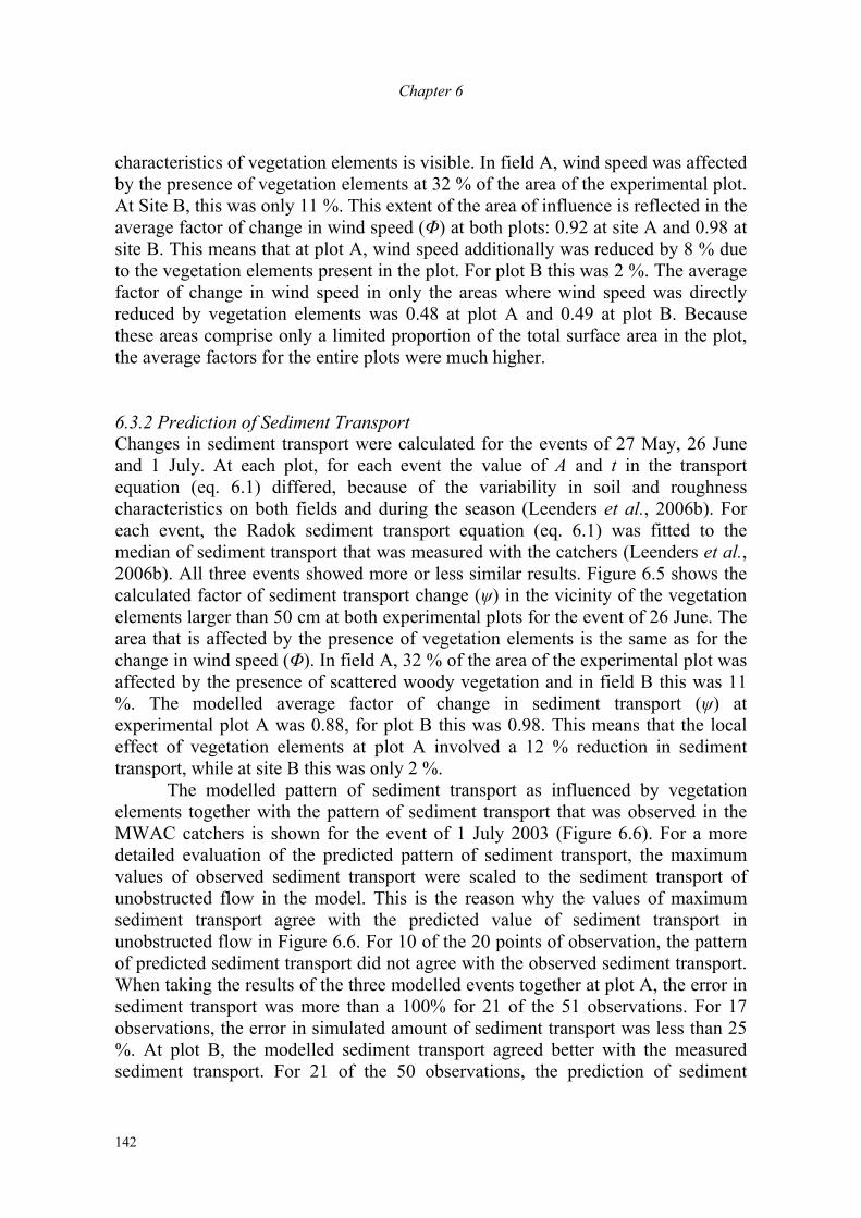
Chapter 6
142
characteristics of vegetation elements is visible. In field A, wind speed was affected by the presence of vegetation elements at 32 % of the area of the experimental plot. At Site B, this was only 11 %. This extent of the area of influence is reflected in the average factor of change in wind speed (Φ) at both plots: 0.92 at site A and 0.98 at site B. This means that at plot A, wind speed additionally was reduced by 8 % due to the vegetation elements present in the plot. For plot B this was 2 %. The average factor of change in wind speed in only the areas where wind speed was directly reduced by vegetation elements was 0.48 at plot A and 0.49 at plot B. Because these areas comprise only a limited proportion of the total surface area in the plot, the average factors for the entire plots were much higher. 6.3.2 Prediction of Sediment Transport Changes in sediment transport were calculated for the events of 27 May, 26 June and 1 July. At each plot, for each event the value of A and t in the transport equation (eq. 6.1) differed, because of the variability in soil and roughness characteristics on both fields and during the season (Leenders et al., 2006b). For each event, the Radok sediment transport equation (eq. 6.1) was fitted to the median of sediment transport that was measured with the catchers (Leenders et al., 2006b). All three events showed more or less similar results. Figure 6.5 shows the calculated factor of sediment transport change (ψ) in the vicinity of the vegetation elements larger than 50 cm at both experimental plots for the event of 26 June. The area that is affected by the presence of vegetation elements is the same as for the change in wind speed (Φ). In field A, 32 % of the area of the experimental plot was affected by the presence of scattered woody vegetation and in field B this was 11 %. The modelled average factor of change in sediment transport (ψ) at experimental plot A was 0.88, for plot B this was 0.98. This means that the local effect of vegetation elements at plot A involved a 12 % reduction in sediment transport, while at site B this was only 2 %.
The modelled pattern of sediment transport as influenced by vegetation elements together with the pattern of sediment transport that was observed in the MWAC catchers is shown for the event of 1 July 2003 (Figure 6.6). For a more detailed evaluation of the predicted pattern of sediment transport, the maximum values of observed sediment transport were scaled to the sediment transport of unobstructed flow in the model. This is the reason why the values of maximum sediment transport agree with the predicted value of sediment transport in unobstructed flow in Figure 6.6. For 10 of the 20 points of observation, the pattern of predicted sediment transport did not agree with the observed sediment transport. When taking the results of the three modelled events together at plot A, the error in sediment transport was more than a 100% for 21 of the 51 observations. For 17 observations, the error in simulated amount of sediment transport was less than 25 %. At plot B, the modelled sediment transport agreed better with the measured sediment transport. For 21 of the 50 observations, the prediction of sediment
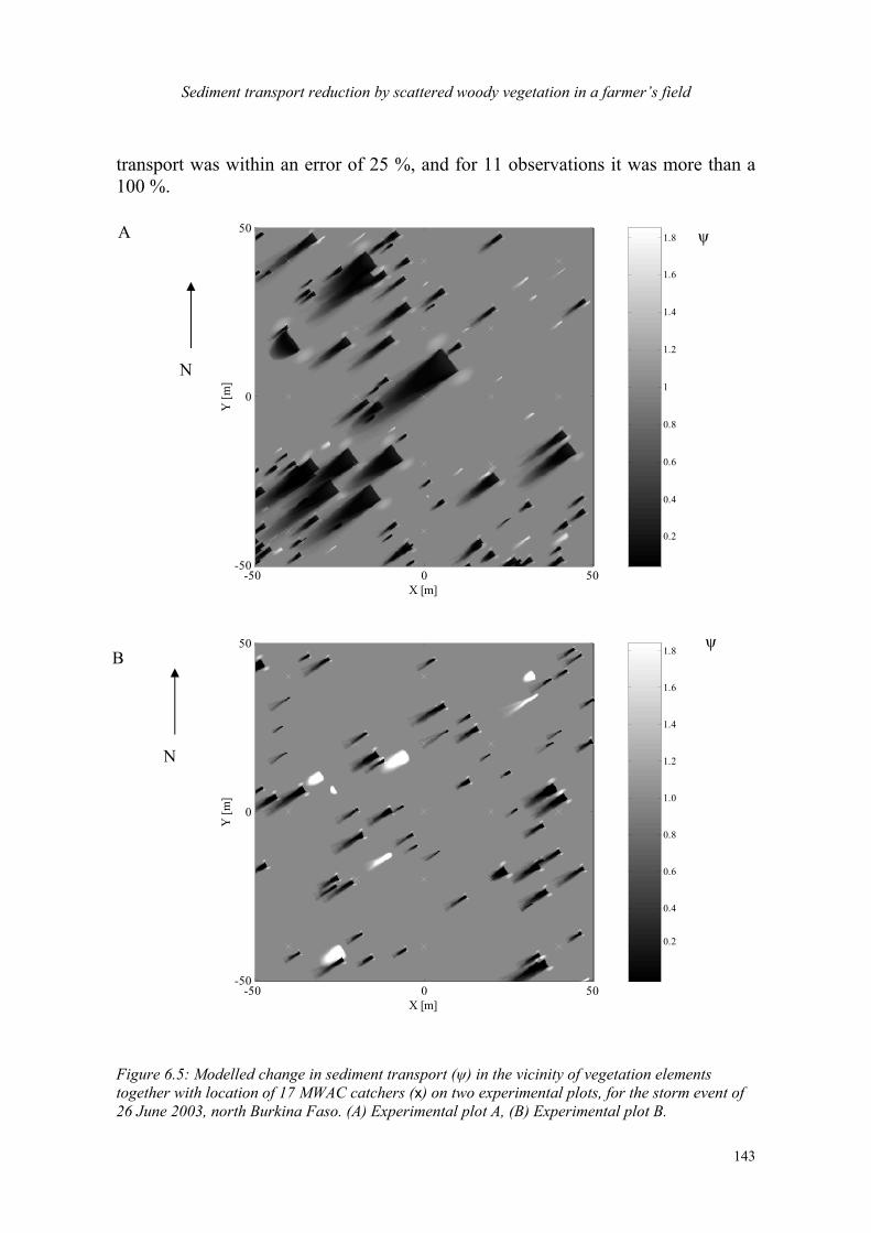
Sediment transport reduction by scattered woody vegetation in a farmer’s field
143
transport was within an error of 25 %, and for 11 observations it was more than a 100 %.
0.2
0.4
0.6
0.8
1
1.2
1.4
1.6
1.8
X [m]
Y [m
]
-50 0 50
50
0
-50
0.2
0.4
0.6
0.8
1.0
1.2
1.4
1.6
1.8
X [m]
Y [m
]
-50 0 50
50
0
-50
Figure 6.5: Modelled change in sediment transport (ψ) in the vicinity of vegetation elements together with location of 17 MWAC catchers (x) on two experimental plots, for the storm event of 26 June 2003, north Burkina Faso. (A) Experimental plot A, (B) Experimental plot B.
N
N
B
A ψ
ψ
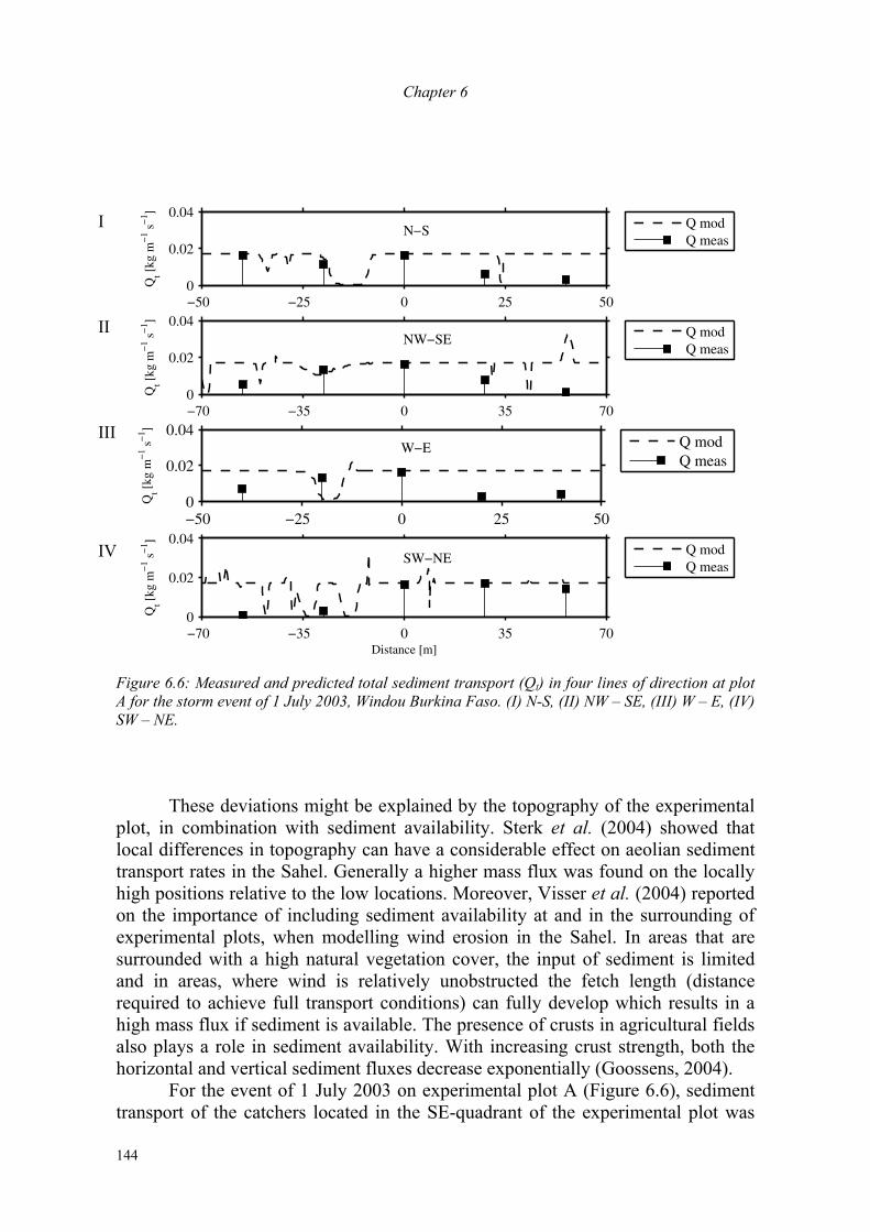
Chapter 6
144
−50 −25 0 25 500
0.02
0.04
Qt [
kg m
−1 s
−1 ]
N−S Q mod
Q meas
−70 −35 0 35 700
0.02
0.04
Qt [
kg m
−1 s
−1 ]
NW−SE Q mod
Q meas
−50 −25 0 25 500
0.02
0.04
Qt [
kg m
−1 s
−1 ]
W−E Q mod
Q meas
−70 −35 0 35 700
0.02
0.04
Distance [m]
Qt [
kg m
−1 s
−1 ]
SW−NE
Q modQ meas
Figure 6.6: Measured and predicted total sediment transport (Qt) in four lines of direction at plot A for the storm event of 1 July 2003, Windou Burkina Faso. (I) N-S, (II) NW – SE, (III) W – E, (IV) SW – NE. These deviations might be explained by the topography of the experimental plot, in combination with sediment availability. Sterk et al. (2004) showed that local differences in topography can have a considerable effect on aeolian sediment transport rates in the Sahel. Generally a higher mass flux was found on the locally high positions relative to the low locations. Moreover, Visser et al. (2004) reported on the importance of including sediment availability at and in the surrounding of experimental plots, when modelling wind erosion in the Sahel. In areas that are surrounded with a high natural vegetation cover, the input of sediment is limited and in areas, where wind is relatively unobstructed the fetch length (distance required to achieve full transport conditions) can fully develop which results in a high mass flux if sediment is available. The presence of crusts in agricultural fields also plays a role in sediment availability. With increasing crust strength, both the horizontal and vertical sediment fluxes decrease exponentially (Goossens, 2004).
For the event of 1 July 2003 on experimental plot A (Figure 6.6), sediment transport of the catchers located in the SE-quadrant of the experimental plot was
I
II
III
IV
Sediment transport reduction by scattered woody vegetation in a farmer’s field
145
largely overestimated. The issue of sediment availability is clearly illustrated for the most SE-catcher in Figure 6.6-II. The catcher was positioned nearby a trunk of a tree, within the area in which wind speed was accelerated. As such a large transport capacity of the wind was expected at this point. However, the observed sediment transport at this location was low. Thus, although sediment transport was possible from an aerodynamic point of view, sediment was not transported because it probably was not available. The reduction in sediment transport in the NW-quadrant is partly explained by the vegetation present (Figure 6.6-II), but the topography also might have played a role.
The storm event of the 1st of July 2003 indicates that the model-performance could possibly be improved by including the aspects of sediment availability and topography. Although the model at present is limited to this respect, the model still serves as a tool to study the effects of vegetation elements wind speed and sediment transport at the local scale and the scale of a field. Despite incomplete, the presented model can simulate the general pattern of sediment transport in a field as influenced by scattered vegetation and offers insight in wind erosion processes at different scales. 6.3.3 Scenario testing Scenarios of different vegetation characteristics and densities were developed and run for the event of 26 June 2003 for the experimental plot of field B. This event was chosen because it was of short duration and had a high average wind speed (Table 6.1). The results of the scenarios that were run are presented in Table 6.3. The change in wind speed and sediment transport was expressed with factors relative to the modelled results for the same event. Factor US stands for the factor of change in average wind speed for the area, due to an alteration in aerodynamic roughness length in the scenario. Factor QS expresses the change in sediment transport of unobstructed flow, because of the change in average wind speed. Factor ψS represents the local changes in sediment transport in the vicinity of the vegetation elements (Figure 6.2 and 6.3). It was calculated by scaling the average ψ factor of the scenario to the average ψ factor that was obtained for the event of 26 June 2003 (which was 0.98). The overall effect on sediment transport (Ω) of a scenario was calculated by dividing the average amount of sediment transport that was modelled using the scenario, with the average amount of sediment transport that was modelled for the event of 26 June 2003. The factor Ω thus comprises both the local effect of vegetation elements (ψS) and the large-scale effect of these elements (QS).
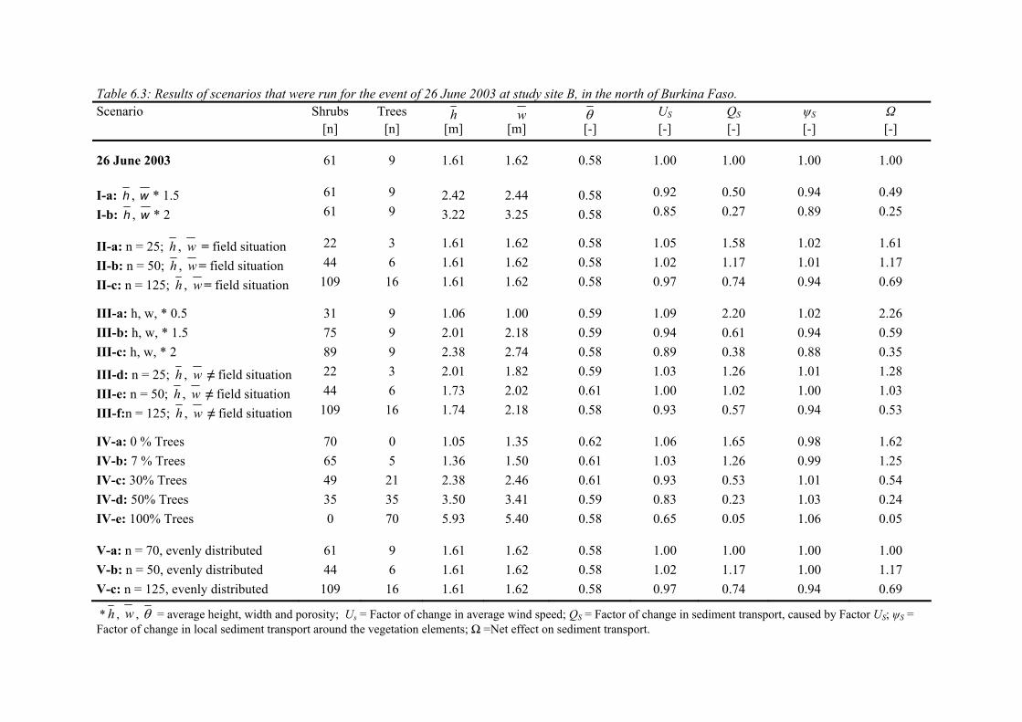
Table 6.3: Results of scenarios that were run for the event of 26 June 2003 at study site B, in the north of Burkina Faso. Scenario Shrubs Trees h w θ US QS ψS Ω [n] [n] [m] [m] [-] [-] [-] [-] [-]
26 June 2003 61 9 1.61 1.62 0.58 1.00 1.00 1.00 1.00
I-a: h , w * 1.5 61 9 2.42 2.44 0.58 0.92 0.50 0.94 0.49
I-b: h , w * 2 61 9 3.22 3.25 0.58 0.85 0.27 0.89 0.25
II-a: n = 25; h , w = field situation 22 3 1.61 1.62 0.58 1.05 1.58 1.02 1.61
II-b: n = 50; h , w = field situation 44 6 1.61 1.62 0.58 1.02 1.17 1.01 1.17
II-c: n = 125; h , w = field situation 109 16 1.61 1.62 0.58 0.97 0.74 0.94 0.69
III-a: h, w, * 0.5 31 9 1.06 1.00 0.59 1.09 2.20 1.02 2.26 III-b: h, w, * 1.5 75 9 2.01 2.18 0.59 0.94 0.61 0.94 0.59 III-c: h, w, * 2 89 9 2.38 2.74 0.58 0.89 0.38 0.88 0.35
III-d: n = 25; h , w ≠ field situation 22 3 2.01 1.82 0.59 1.03 1.26 1.01 1.28
III-e: n = 50; h , w ≠ field situation 44 6 1.73 2.02 0.61 1.00 1.02 1.00 1.03
III-f:n = 125; h , w ≠ field situation 109 16 1.74 2.18 0.58 0.93 0.57 0.94 0.53
IV-a: 0 % Trees 70 0 1.05 1.35 0.62 1.06 1.65 0.98 1.62 IV-b: 7 % Trees 65 5 1.36 1.50 0.61 1.03 1.26 0.99 1.25 IV-c: 30% Trees 49 21 2.38 2.46 0.61 0.93 0.53 1.01 0.54 IV-d: 50% Trees 35 35 3.50 3.41 0.59 0.83 0.23 1.03 0.24 IV-e: 100% Trees 0 70 5.93 5.40 0.58 0.65 0.05 1.06 0.05
V-a: n = 70, evenly distributed 61 9 1.61 1.62 0.58 1.00 1.00 1.00 1.00 V-b: n = 50, evenly distributed 44 6 1.61 1.62 0.58 1.02 1.17 1.00 1.17 V-c: n = 125, evenly distributed 109 16 1.61 1.62 0.58 0.97 0.74 0.94 0.69
* h , w , θ = average height, width and porosity; Us = Factor of change in average wind speed; QS = Factor of change in sediment transport, caused by Factor US; ψS = Factor of change in local sediment transport around the vegetation elements; Ω =Net effect on sediment transport.
Sediment transport reduction by scattered woody vegetation
147
Type I scenarios tested the effect of the average silhouette area of the vegetation elements present in the experimental plot. The height and width of the vegetation elements that were taken into account in the field situation were multiplied with a constant factor. With increasing silhouette area, the net change in sediment transport (Ω) decreased exponentially. With Type II-scenarios the effect of the number of vegetation elements was tested. The percentage of trees and the average characteristics of the vegetation elements stayed the same as in the field situation. The location of the vegetation elements in the plot was chosen randomly. In this scenario, Ω seemed to reduce exponentially as well, although the exponential decline is less compared with Type I scenarios.
In scenario Type III both the silhouette area and the number of vegetation elements changed. In scenarios III-a, III-b and III-c the height and width of all vegetation elements that were observed in the experimental plot were multiplied with a constant factor. By doing this, the percentage of trees and the number of vegetation elements changed in these scenarios. For example, in the original run of 26 June, a vegetation element of 0.4 m height was not taken into account because it was smaller than 0.5 m. In scenario III-b and III-c, this element was taken into account because the height was multiplied with a factor 1.5 and 2, respectively, resulting in a height larger than 0.5 m. The results of scenarios III-a, III-b and III-c showed also an exponential decrease in sediment transport (Ω), but the exponential decrease is less than in scenario Type I. Despite the larger number of vegetation elements in scenario III-b and III-c, these scenarios resulted in a larger factor of Ω, than scenario Type I-a and I-b. This was related to the lower silhouette area of scenario III-b and III-c compared to scenario I-a and I-b (Table 6.3).
A more realistic situation of changing the number and characteristics of vegetation elements was simulated in scenarios III-d, III-e and III-f. In these scenarios, the characteristics of the vegetation elements were generated randomly from the vegetation database of the entire field. The percentage of trees was the same as in the field situation and the location of the vegetation elements in the plot was chosen randomly. Scenarios III-d, III-e and III-f showed a linear decrease in factor Ω with increasing number of vegetation elements. In scenario III-e, the number of vegetation elements was decreased with almost 30 % (from 70 to 50), but the model simulated a sediment transport that differed only 3 % with the modelled sediment transport in the real field situation. This was related to a larger silhouette area in scenario III-e, compared to the field situation. Apparently the increase in wind speed due to a decrease in number of vegetation elements was more or less counterbalanced by the decrease in wind speed due to an increase in silhouette area.
Type IV scenarios tested the effect of the ratio of tree-type vegetation elements to shrub-type vegetation elements. The number of vegetation elements in these scenarios was equal to the number of elements in the field situation (Table 6.3). By increasing the percentage of trees, the silhouette area increased (Table 6.3) and average wind speed and sediment transport decreased. Although, locally in the field sediment transport was increased due to the increase of wind speed around the
Chapter 6
148
trunk of trees (ψS is larger than 1 in scenario IV-c, IV-d and IV-e), this effect seems insignificant when comparing it to the effect these large vegetation elements exert on the sediment transport by affecting the wind speed for the entire field (QS). For example, for a tree percentage of 30 % the model simulated an increase in the local sediment transport in the plot (ψS) with 3 %. However, due to the changes in the average wind speed (US), the amount of sediment transport in unobstructed flow (QS) decreased 77 %. The net effect of this scenario (Ω) was a reduction of 76 % in sediment transport compared to the field situation.
Scenario Type IV clearly indicates that the presence of trees is important in influencing sediment transport in an area. Trees are large objects and as a consequence the number of trees in an area has an important effect on the average silhouette area in an area (Table 6.3). The US factors of scenario type IV-a and IV-b, show that trees are more effective in extracting momentum from the air and reducing the average wind speed in an area than shrubs. In scenario IV-a, factor US increased 6 % as a result of removing the 9 trees present in the area. In scenario IV-b, 4 of the 9 trees were removed, resulting in an increase of 3 % in the average wind speed. This illustrates the crucial role trees have in the parkland system, with respect to reducing the average wind speed in an area.
A final scenario was run on the arrangement of vegetation elements in a field. It was checked whether vegetation elements that are evenly distributed in the field would result in a lower sediment transport compared to vegetation elements that are randomly scattered in the field. The modelled results of scenario V-a, V-b and V-c are exactly the same as respectively those of the field situation, scenario II-b and scenario II-c. This indicates that there is no difference in effect of spatial distribution when vegetation is evenly or randomly distributed, when considering scattered vegetation. This result is not surprising, as the density in scattered vegetation is generally so low, that obstacles act in isolation and wind speed reduction zones do not interfere much with each other (Figure 6.4B).
From the performed scenarios two general features become clear. First, the scenarios showed that the local effect of trees and shrubs on sediment transport (ψS) varied less than the effect these vegetation elements exerted on sediment transport through affecting the average wind speed in an area (QS) (Table 6.3). In the model, the vegetation elements in the tested scenarios altered the sediment transport in their vicinity (ψS) up to 11 % (scenario I-b). The effects on sediment transport due to the change in the wind profile were an order of magnitude larger (120 % in scenario III-a).
Although the local effects of vegetation elements are less than the large-scale effects, it can not be concluded that the local effects of vegetation elements on sediment transport are not important. Due to the ‘local effects’, e.g. the enrichment of the soil by trapping of sediment by shrubs, the crop production might locally increase (Sterk et al., 2004). For a farmer this is extremely important. However, the scenario runs indicate that average sediment transport in a field is much more affected by the vegetation elements in upwind areas than by the vegetation elements that are actually present in the field. The possibility of sediment transport
Sediment transport reduction by scattered woody vegetation
149
reduction one can achieve in a field, by managing the natural woody vegetation present in this field is thus limited. Therefore, a farmer who wants to diminish the sediment transport in his field(s) effectively has to ensure that vegetation elements are present in areas upwind of his field(s). Because of the variable wind direction of storm events, the location of upwind fields differs. This means that for an effective reduction in sediment transport in one field, vegetation elements have to be present in fields surrounding this field. As such it is concluded that using natural woody vegetation as a wind erosion control strategy involves collaboration between farmers. Therefore it is recommended to regenerate and manage woody vegetation at the scale of at least a village. This coincides well with a popular community-based resource management approach in the Sahelian region practiced since the mid-1980s. This village land management approach, commonly referred to as the “Gestion de Terroirs Villageois”, is characterized by a consideration of social and institutional factors in resource management. It also intends to authorize local communities with resource management and utilizes local knowledge through participatory projects (Turner, 1999).
A second feature that can be deduced from the scenarios is that different combinations of vegetation characteristics and number of vegetation elements present in an area result in the same change of sediment transport. An increase in the number of vegetation elements from 70 to 125 (scenario III-f) resulted in the same reduction in sediment transport as an increase of percentage of trees from 13 % to 30 % (scenario IV-c). A decrease in the number of vegetation elements from 70 to 25 (scenario II-a) resulted in the same reduction in sediment transport as a situation in which no trees were present (scenario IV-a). Thus the combination of characteristics of vegetation elements in a field determines the protection of scattered vegetation for sediment transport. Rather than one optimum there is a range of combinations in silhouette area, type of vegetation elements (trees and shrubs) and the density of vegetation elements that determine the extent of change in sediment transport. The best reduction in sediment transport is obtained by a combination of a high number of vegetation elements, a high percentage of trees and a large silhouette area. However, it is obvious that a farmer is not willing or able to meet these criteria. For example, farmers might not want to have more than a certain number of vegetation elements within their fields because they fear competition for water, light and nutrients with the main crop. The reduction in sediment transport that is achievable in a specific situation, therefore, is also subject to boundary conditions inherent to the farming system and specific needs and interests of farmers.
Chapter 6
150
6.4 Conclusions The model presented in this study was based on a model that was developed for a single shrub-type vegetation element. The latter model was tested for an isolated shrub, for which it simulated the change in wind speed and sediment transport reasonably well (Leenders et al., 2006b). Here, the model has been adapted to apply it to the field scale, and used to study the effects of different scenarios on sediment transport. The model of Lettau (1969) was taken to incorporate the effects vegetation elements exert on the aerodynamic roughness and average wind speed in an area. However, the validity of Lettaus’ model is not widely proven. Therefore a first step in improving and validating the presented model of this study would be to test the validity of Lettaus’ model in a range of sparsely vegetated terrains.
Field measurements on sediment transport during three storms on two experimental plots showed that the model of this study could also be improved by expanding it with the aspects of topography and sediment availability in fields. In addition the applicability and usability of the model would enhance when a general sediment transport equation would be available to predict sediment transport. This latter issue remains a topic of research. Despite these limitations, the developed model serves as a tool to provide insight in the effects vegetation elements exert on sediment transport on different scale levels.
The scenario runs clearly illustrated that considerable effects in sediment transport can be obtained with relatively small changes in vegetation characteristics (e.g. scenario II-b and IV-b, compared to the field situation). It was also illustrated that the large-scale effects of vegetation elements on sediment transport i.e. the effects on sediment transport by influencing the average wind speed in an area outweigh the small scale effects vegetation elements exert in their vicinity. Especially trees appeared to be very effective in affecting the average wind speed in an area by extracting momentum from the air. It is concluded that the regeneration and management of scattered vegetation has to be approached at the scale of a village or community, when using natural woody vegetation as a wind erosion control strategy. The change in sediment transport obtainable by a farmer in his field alone is an order of magnitude less than the change in sediment transport that can be obtained with more trees in upwind areas.
In addition, the model showed that there is a range of characteristics of vegetation elements that diminish sediment transport to a certain extent. The extent of reduction in sediment transport depends on a combination of the silhouette area, the type of vegetation element (shrubs and trees) and the density of vegetation elements. The highest reduction in sediment transport would be obtained with a large number of vegetation elements, a large percentage of trees in upwind areas and a large silhouette area. However, the reduction in sediment transport that is achievable in a farmers’ field is also subject to boundary conditions inherent to the farming system or the farmer himself. Although the extent of change in sediment transport by the use of vegetation elements is variable and the implementation might differ per farming system, the
Sediment transport reduction by scattered woody vegetation
151
strategy of using scattered vegetation to diminish sediment transport will be applicable to a range of situations. By using vegetation as a wind erosion control measure, farmers are not forced to adopt measures which are new to them or require additional labour. Also there is no need to use specific species or give up or change practices they are already familiar with. These aspects combined with the willingness of farmers to adopt soil conservation measures (Visser et al., 2003) leads to the conclusion that the use of scattered vegetation, the so-called parkland-system in the Sahel, as a wind erosion control technique is promising. References Baidu-Forson J., Napier T.L. 1998: Wind erosion control within Niger. Journal of Soil and Water
Conservation 53: 120-125. Bielders C.L., Michels K., Rajot J.L. 2000: On-farm evaluation of ridging and residue
management practices to reduce wind erosion in Niger. Soil Science Society of America Journal 64: 1776-1785.
Bielders C.L., Alvey S., Cronyn N. 2001: Wind erosion: The perspective of grass-roots communities in the Sahel. Land Degradation & Development 12: 57-70.
Boffa J.M. 1999: Agroforestry parklands in sub-Saharan Africa. FAO Conservation Guide 34 FAO, Rome. 231 pp.
Brutsaert W. 1982: Evaporation into the Atmosphere: Theory, History and Applications. Springer. Dordrecht, The Netherlands. 316 pp.
Goossens D. 2004: Effect of soil crusting on the emission and transport of wind-eroded sediment: field measurements on loamy sandy soil. Geomorphology 58: 145-160.
Goossens D., Offer Z., London G. 2000: Wind tunnel and field calibration of five aeolian sand traps. Geomorphology 35: 233-252.
Greely R., Iversen J.D. 1985: Wind as a Geological Process. Cambridge University Press. Cambridge, UK. 333 pp.
Hagen L.J. 1998: WEPS: Wind Erosion Prediction System. Wind Erosion Research Unit. Kansas State University, USA.
Kenney W.A. 1987: A Method for estimating windbreak porosity using digitized photographic silhouettes. Agricultural and Forest Meteorology 39: 91-94.
Lamers J.P.A., Michels K., Feil P.R. 1995: Wind erosion control using windbreaks and crop residues: Local knowledge and experimental results. Der Tropenlandwirt, Beiträge zur tropischen Landwirtschaft und Veterinärmedizin 96: 87-96.
Le Houérou H.N. 1997: Climate, flora and fauna changes in the Sahara over the past 500 million years. Journal of Arid Environments 37: 619-647.
Leenders J.K., Visser S.M., Stroosnijder L. 2005a: Farmers' perceptions of the role of scattered vegetation in wind erosion control in Burkina Faso. Land Degradation & Development 16: 327 - 337.
Leenders J.K., van Boxel J.H., Sterk G. 2005b: Wind forces and related saltation transport. Geomorphology 71: 357-372.
Leenders J.K., Boxel J.H., Sterk G. 2006a: The effect of single vegetation elements on wind speed and sediment transport in the Sahelian zone of Burkina Faso. Accepted for publication in: Earth Surface Processes and Landforms.

Chapter 6
152
Leenders J.K., Sterk G., Visser S.M., Boxel J.H. 2006b: Modeling the effects of single vegetation elements on wind-blown sediment transport. Submitted to: Earth Surface Processes and Landforms.
Lettau H. 1969: Note on Aerodynamic Roughness-Parameter Estimation on the Basis of Roughness-Element Description. Journal of Applied Meteorology 8: 828-832.
Lloyd C.R., Gash J.H.C., Sivakumar M.V.K. 1992: Derivation of the Aerodynamic Roughness Parameters for a Sahelian Savannah Site using the Eddy Correlation technique. Boundary Layer Meteorology 58: 261-271.
Michels K., Sivakumar M.V.K., Allison B.E. 1995: Wind erosion control using crop residue I. Effects on soil flux and soil properties. Field Crops Research 40: 101-110.
Mohammed A.E., Stigter C.J., Adam H.S. 1995: Moving sand and its consequences on and near a severely desertified environment and a protective shelterbelt. Arid soil Research and Rehabilitation 9: 423-435.
Petersen R.L. 1997: A wind tunnel evaluation of Methods for Estimating Surface Roughness Length at Industrial Facilities. Atmospheric Environment 31: 45-57.
Petit S. 2003: Parklands with fodder trees: a Fulbe response to environment and social changes. Applied Geography 23: 205-225.
Radok U. 1977: Snow drift. Journal of Glaciology 19: 123-139. Raupach M.R., Thom A.S., Edwards I. 1980: A wind-tunnel study of turbulent flow close to
regularly arrayed rough surfaces. Boundary Layer Meteorology 18: 373-397. Reij C., Tappan G., Belemvire A. 2005: Changing land management practices and vegetation on
the Central Plateau of Burkina Faso (1968-2002). Journal of Arid Environments 63: 642-659.
Rinaudo T. 1996: Tailoring wind erosion control methods to farmers' specific needs. pp 161-171. In: B. Buerkert, et al. (Eds.). Proceedings of the International Symposium on 'Wind Erosion in West Africa: The Problem and its Control', Germany, 5-7 December 1994. Margraf Verlag, Weikersheim, Germany.
Ruck V.B., Schmitt F. 1986: Das Strömungsfeld der Einzelbaumuströmung. Abschätzung von Depositionswahrscheinlichkeiten für Feinsttröpfchen. Forstwissenschaftliches Centralblatt 105: 178-196.
Spaan W.P., Van den Abeele G.D. 1991: Wind borne particle measurements with acoustic sensors. Soil Technology 4: 51-63.
Sterk G. 2000: Flattened residue effects on wind speed and sediment transport. Soil Science Society of America Journal 64: 852-858.
Sterk G., Raats P.A.C. 1996: Comparison of models describing the vertical distribution of wind-eroded sediment. Soil Science Society of America Journal 60: 1914-1919.
Sterk G., Spaan W.P. 1997: Wind erosion control with crop residues in the Sahel. Soil Science Society of America Journal 61: 911-917.
Sterk G., Haigis J. 1998: Farmers' knowledge of wind erosion processes and control methods in Niger. Land Degradation & Development 9: 107 - 114.
Sterk G., Stein A., Stroosnijder L. 2004: Wind effects on spatial variability in pearl millet yields in the Sahel. Soil &Tillage Research 76: 25 - 37.
Taylor-Powell E. 1991: Integrated management of agricultural watersheds: Land tenure and indigenous knowledge of soil and crop management. Tropical Soils Bulletin 91-04 Texas A&M University: College Station, TX.
Turner M.D. 1999: Conflict, Enviromental Change, and Social Institutions in Dryland Africa: Limitations of the Community Resource Management Approach. Society & Natural Resources 12: 643-657.
Valentin C. 1995: Sealing, crusting and hardsetting soils in Sahelian agriculture. pp 53-76. In: So H.B. et al. (Ed.) Sealing, Crusting and Hardsetting Soils: Productivity and Conservation. Australian Society of Soil Science, Brisbane, Australia.
Sediment transport reduction by scattered woody vegetation
153
Van Boxel J.H., Sterk G., Arens S.M. 2004: Sonic anemometers in aeolian sediment transport research. Geomorphology 59: 131-147.
Visser S.M., Leenders J.K., Leeuwis M. 2003: Farmers' perceptions of erosion by wind and water in northern Burkina Faso. Land Degradation & Development 14: 123- 132.
Visser S.M., Sterk G., Snepvangers J.J.J.C. 2004: Spatial variation in wind-blown sediment transport in geomorphic units in northern Burkina Faso using geostatistical mapping. Geoderma 120: 95-107.
Wieringa J. 1976: An objective exposure correction method for average wind speeds measured at a sheltered location. Quarterly Journal of the Royal Meteorological Society 102: 241-253.
Wieringa J. 1993: Representative Roughness Parameters for Homogenous Terrain. Boundary Layer Meteorology 63: 323-363.
Yamba B., Mahamane L., Abdou H., Reij C. 2005: Rapport Etude de Pilote Niger (25 janvier au 10 février 2005). International Resources Group (IRG) Comité Inter-Etats de Lutte contre la Sécheresse au Sahel (CILSS). 30 pp.


Curriculum Vitae
Jakolien K. Leenders was born on the 1st of October 1975, in Deventer, The Netherlands. She grew up in Harderwijk, and attended the secondary school ‘Christelijk College Nassau Veluwe’ in Harderwijk. In 1994 she went to Utrecht to study physical geography at the Utrecht University. For her Masters, she went to the south of France to study the effect of agricultural practices on overlandflow in a small catchment. In 1997 she traveled to Guyana for a practical work on the nutrient cycle in the tropical rainforest. After her studies Jakolien followed a study, to become a geography teacher, and in December 2000 she got the opportunity to start her PhD at the group of Erosion and Soil & Water Conservation at Wageningen University. For her PhD she studied the effect of scattered natural woody vegetation on the process of wind erosion in the Sahelian Zone of Burkina Faso. Between 2001 and 2005 she traveled four times to Burkina Faso, spending in total about 1.5 years in Burkina Faso, where she collaborated with l’Institut de l’ Environnement et des Recherches Agricoles (INERA). Within her PhD, she followed several postgraduate courses, and participated in international congresses. She also supervised several MSc students. This thesis, together with other publications, is the final outcome of her PhD-research. In 2004 and 2006 Jakolien was a member of the ‘Third Chamber’, a shadow parliament dealing with international cooperation and sustainable development. She was working on the topics of microfinance, fair trade and agriculture. After her PhD, Jakolien will start working at HKV consultants in Lelystad, a consultancy company, providing consultancy and research services in the field of water management and water management related problems. She will be appointed as a consultant catastrophe management and will work on data-analysis, risk management and scenario-testing. Jakolien can be contacted at: [email protected]

PE&RC PhD Education Statement Form With the educational activities listed below the PhD candidate has complied with the educational requirements set by the C.T. de Wit Graduate School for Production Ecology and Resource Conservation (PE&RC) which comprises of a minimum total of 22 credits (= 32 ECTS = 22 weeks of activities) Review of Literature (4 credits)
- Wind erosion protection by dispersed trees and shrubs in the Sahelian Zone of Burkina Faso (2001)
- Presentations at Erosion Soil and Water Conservation group (2001) Post-Graduate Courses (3 credits)
- Design and setup of research on wind erosion (2001) - Scientific writing (2002)
Deficiency, Refresh, Brush-up and General Courses (7.5 credits) - French language (2001) - Software course – Endnote (2001) - Fluid mechanics (2001) - Simulation of ecological processes (2001) - Processes and models (2001) - Organizing and supervising thesis work (2001)
PhD Discussion Groups (5 credits)
- Sustainable land-use and resource management (2000-2005) - Statistics, maths and modelling in production ecology and resource conservation (2000-2005)
PE&RC Annual Meetings, Seminars and Introduction Days (0.75 credits) - PE&RC annual meeting: “Food insecurity” (2001) - Effects of climate change on nature (2003) - PE&RC annual meeting: “The truth of science” (2005)
International Symposia, Workshops and Conferences (4 credits) - Soil degradation in Africa, Wageningen (2002) - Annual meeting WOTRO, Amsterdam (2002) - Forum de Recherche Scientifique et des Innovations Technologiques (FRSIT), Ouagadougou,
Burkina Faso (2002) - European geophysical union, 1st general assembly Nice, France (2004) - Workshop sustainable land management in the Sahel (Dori, Burkina Faso) (2005)
Laboratory Training and Working Visits (3 credits) - Laboratory experiments on the airflow pattern around a single object at the I.C.E. Wind
tunnel for wind and water interaction research at Ghent University (2003)
