INTERNATIONAL JOURNAL FOR NUMERICAL METHODS I N ENGINEERING, VOL. 29,633-645 (1990)

A SURFACE FITTING METHOD FOR THREE DIMENSIONAL SCATTERED DATA

CONSTANTINOS A. BALARAS. AND SHELDON M . JETER

The George W. Woodrtfl School of Mechanical Engineering, Georgia Institute of Technology, Atlanta, Georgia 30332, U.S.A.

SUMMARY A method is presented that may be used to empirically establish the type of relationship that is present between a response variable and its influencing factors, by fitting a mathematical model to three dimensional scattered data. The generated response surface is composed of continuous triangular planes that are fitted to the corresponding data in the least squares sense. The method may be easily implemented. It requires some fairly large number of scattered data, two initial boundary conditions and a desired accuracy for the band-wise partitioning of the data. The proposed surface fitting technique has been successfully applied to solar radiation modelling for a number of different data combinations.

1. INTRODUCTION

Development of empirical models from available data often requires the development of a cor- relation between three variables. Some procedures are then required that may be used to investigate the relationship that is present between the response variable (z) and its influencing factors (x) and (y). The response variable (2 ) is the quantity whose value is assumed to be affected by changing the levels of the factors. The factors are the input variables, (x) and ( y), whose values are readily available. Presumably, if one changes the values of the factors, the value of the response varies as well.

The model described in this paper is based on a procedure for fitting a continuous surface through (x, y, z) data. The objective of a three variable study is to account for the significance of both independent variables (x, y) to predict the dependent variable (2). The proposed technique can be applied to any surface fitting problem that generates a response surface from scattered three dimensional data.

Most of the traditional triangulation techniques do not easily lend themselves to applications in which high surface accuracy is not the main objective. For example, methods used for such applications as in the case of Computer Aided Geometric Design (CAGD), picture production and geological applications offer a high degree of intricacy but are of little interest in our study. The development of a correlation between the available variables has to remain simple in order to facilitate future engineering applications.

For reference though, let us list some of these methods. The principles of surface fitting presented by Lancaster and Salkauskas' offer an excellent introductory overview on the subject.

*Current affiliation: Senior Mechanical Engineer, American Standards Testing Bureau, Inc., 1075 Dehaven Avenue, West Conshohocken, PA. 19428, U.S.A. Mailing address: Sot. Charalabi 5, 11472 Athens, Greece

0029-598 1 /90/030633-13SO6.50 0 1990 by John Wiley & Sons, Ltd.

Received 4 February I989 Revised 5 July I989

634 C. A. BALARAS AND S. M. J iTER

Farin’ developed an algorithm that uses triangular Bernstein-Bezier surfaces applicable for CAGD applications. Sloan3 has proposed an algorithm for conducting Delaunay triangulations in the plane, with improved run time.

Correc and Chapuis4 have also dealt with triangulation of scattered data in a Delaunay’s sense suitable for digital terrain modelling. This method is primarily of interest to geologists and geographers for developing maps from geographical data bases. A survey of some surface fitting methods by Barnhill’ covers several modelling approaches to the detail design of bivariate surfaces.

2.. DEVELOPMENT OF A SURFACE FITTING ALGORITHM

The method developed utilizes a discrete data set of three variables, (x, y , z), to fit through these data a continuous surface composed of appropriate size quadrilateral planes. The method calls for an initial specification of some fairly large number of scattered data, lying in a bounded three dimensional space. Measured data usually have errors which have to be smoothed out. One way to reduce the noise inherent in the raw data is to fit the approximating function by the method of the least squares.

To start, the three dimensional data are broken down into x and y bands, of appropriate width each. This creates a number of working spaces shown in Figure 1. For every rectangular space that is created by the band partitioning of the (x, y) plane, the bounded data are identified and collected. These rectangular planes are called patches.

Each quadrilateral patch can be broken down to two triangular patches; an upper triangular patch (U-patch), and a lower triangular patch (L-patch). The numbered corner points marked in Figure 1 are called nodes, connecting the patch boundaries. These triangular patches may then be fitted to the appropriate data within the given patch boundaries in the least squares sense.

The resulting surface is composed of an assembly of patches. To ensure that adjacent patches are continuous across their contiguous boundaries, some boundary conditions have to be imposed. It becomes quite clear that our method must not only fit surface patches to the corresponding data, but also blend fitted predefined patches together.

Every triangular patch has two known nodes (all three co-ordinates specified) and one unknown node (z co-ordinate unspecified). The third node is fully defined by fitting a given

1 3 9 13 x

Figure 1. Band wise sweeping process for triangulated patch generation on the (x-y) plane

SURFACE FITIMG FOR 3-D DATA 635

triangular patch to the appropriate data in the least squares sense. The existence, though, of lower and upper patches suggests that for convenience a standard approach should be developed to perform the fitting procedures.

A solution to this problem is achieved by establishing a fixed co-ordinate system (X, Y, Z). This would require the development of a w r d i n a t e transformation procedure to relate, for example, the (x, y, z) co-ordinates to an ( X , Y, Z) co-ordinate system.

One such transformation is illustrated with the following example, based on our (x, y, z) data. Consider three nodes: ( x , , y , , zl), (x,, y,, z2) and (x3 , y 3 , z3). The axes are rotated through an angle 8 about the origin located at point 1, as shown in the two dimensional (x, y) representation in Figure 2.

From basic trigonometry the following relations between the two co-ordinate systems were obtained:

Y CosO + X sine = y - y , = Sy (1 1 - ~ ~ i n e + x ~ ~ e = ~ - x , = ~ x (2)

(3)

(4)

z = z - z , (5 )

The solution for the two equations system becomes

x = by sine + bx m e Y = by me - bx sine

while for the z co-ordinate the relationship is simply

Thus, for a given triangular patch all the data and known nodes with co-ordinates (x, y, z) can be mapped to the standard X-Y-Z co-ordinate system through equations (3) to (5). The known vertices of the triangular patch are located at (0, 0,O) and ( X , , 0, Z2), while the third node is located at ( X 3 , Y 3 , Z3), as shown in Figure 2.

The objective is to determine Z , through a least squares minimization. The fitting of a tnangu- lar plane can always be done on the standard (X, Y, Z) co-ordinate system and then transformed to any given co-ordinate system. The equation of a plane passing through these three points can

Y

X

Figure 2. Mapping and trigonometric relations between the original (x, y, z) d n a t c system a d the slrodvd (X, Y, Z) co-ordinate system

636 C. A. BALARAS AND S. M. JETER

X Y Z 0 0 0 1

= x , 0 z , x, y3 z3

x, 0 z, 1

be expressed as

= o

x - X I y-yy, z - z i

x 2 - x 1 y , - y , z 2 - z 1

x3 - x 1 Y3 - Y 1 z3 - 2 1

Equation (6) can be reduced to

= o

The residual for a point is defined as the distance of a data point from the (X17 Y,, Z l ) , ( X 2 , Y,, Z,)7 (X,, Y , , Z , ) plane, and can be expressed as

ci = di - z or IE! = C ( d i - 2)’

where di = distance of (Xi, Yi, d i ) data from plane, Z = elevation of data on the plane according to equation (7).

The least squares minimization then requires that

which results in an expression for Z , ,

z , =

where Xi, Yi , di = data co-ordinates, X,, Z, = co-ordinates of second node (Y, = 0) and X , , Y , = known co-ordinates of third node.

The next step would be to map the calculated Z , co-ordinate in the reverse direction, from the standard system onto the original co-ordinate system, according to equation (5).

The three nodes (xl, y , , zl) , (x,, y,, z , ) and (x3, y,, z,) now completely define a triangular plane of the form

where x, y, z = data co-ordinates bounded into the specified triangular plane between nodes 1, 2 and 3.

Once an L-patch has been fixed, the common boundary nodes with the U-patch are used to repeat the process for the third unspecified node of the U-patch. The result is a fully specified rectangular patch. Blending is achieved through successive patch generation. The newly gene- rated patch must satisfy the boundary conditions of its previously defined neighbour. Once the

SURFACE FITTING FOR 3-D DATA 637

first patch is generated, the next patch on the same x band may be generated, and so on. The same procedure is repeated for the following (x) bands.

Moving to the second (x) band, first we observe from Figure 1 that all nodes along the left side boundary have already been fixed from the previous sweep, while the right side boundary nodes are unspecified. Repeating the same procedure along the second (x) band, one can initially specify nodes 9 and 10, in that order. The next lower triangular patch has already its three nodes (4, 10 and 6) fixed by our previous calculations.

As we proceed, the same problem arises with all remaining lower triangular patches. This of course means that the data bounded within these patches were not directly accounted for, or in a sense were ‘lost’. Thus, the method discussed up to this point may use only a fraction of the available data.

The next logical step was to alter the method developed thus far in such a way that all data are accounted for. Figure 1 may be used again here to help us visualize the new procedure. The upper triangular patches adjacent to fixed lower ones should attract our attention.

For example, consider the (4,5,6} U-patch. At this point nodes 4 and 5 are known. Previously node 6 was to be calculated based only on the data enclosed by (4,5,6}. This time, the data from the lower triangular patch (4,6, lo}, of the adjacent (x) band, are also going to be incorporated in the calculations, weighted though as one half.

A least squares minimization was performed to the grouped data. The corresponding sum of squares of the residuals is now composed of two components. The first originates from the data enclosed in the upper triangular patch and is denoted by &a. The second component originates from the appropriate data of the adjacent L-patch and is denoted by

A minimization was then performed on the sum of the sums, weighting each term accordingly, CE; + $ ~ E E . Again we require that,

which results to a new expression for Z,,

where (XW, Yui, dui) = data co-ordinates from the U-patch, and (XLi, YLi, dL1) = data co-ordinates from the L-patch.

The procedure is repeated for every U-patch of all (y) bands, except the first one, using the data from the L-patch of their adjacent (x) bands.

3. ALTERNATIVE SURFACE FITTING METHODS

For completeness, one needs some other fitting techniques to which our method may be compared (a task undertaken in a later section). There are several software libraries that provide

638 C. A. BALAllAs A N D S M IETER

algorithms for surface fitting to three dimensional data- For example, the general purpose mathematical library, International Mathematical and Statistical Libraries (IMSL),“ includes usefd facilities for surf= fitting

The IMSL Eibrary provides a merdabk subroutine tbat perfom smooth surfacre fitting to irrcgubrly distributai data points. The routiae cahiates an interpolating function wbich is a fiftb-degree polynomial m each h g k of a trianguIation of the (x, y) projection of the surface The interpolation function is continuous and has continuous first-order partial derivatives Tbe feadtt may refer to References 6 and 7 for more details. Note, though, that this method ir difficult to implement owing to its large memory requirements of 31N (N total number of data). In general, polynomial corrdations on two independent variables are easy to bpkment, since

an RMS solution for the polynomial coefficients may completely define the correlation. However, a potpnomial fit to a cornpiex s p r f a ~ e is subject to general ditficultiq such as oscillations, and the deveIoped surface is not locally weighted. In addition, whenever large regions of the respoose variable are zero, a polynomial method w& tend to cause negative divergences that are often erroneous.

An alternative surface fit may be s u c a d d l y performed with the use of DISSPLA.* The user must provide a doubtedimensioned array amtainmg the elevations (z values) that describe the surface to be fitted. Available routines may be used to generate an evenly spaced grid from irregdar sets of x, y, z data.

The algorithm to prepare a regular matrix of z values is a mathematical weighting technique based on the distance from a grid node to the irregular spaced data points in its selected ‘search area’. This technique is an inversely weighted fit over a search area, which is simply stated by

where zit = value to be computed for node jk of the grid, Di = distance from the node jk to the irregular point zir w = weighting factor, and n = number of irregular points which fall in the ‘search area’ for the irregular point zi.

By defining a ‘search area’, the method first finds which cell the irregular point Pi lies in. It then looks two cells to the left (counting the cell it is currently in, as one), two cells to the right, two cells below and two cells above, for any irregular points (P,) to consider in the weighting equation. This forms a nine cell search area.

Depending on the search area, the method has the advantage of being locally weighted. However, DISSPLA does not result in an analytically defined surface that may be precisely reproduced or manipulated by integration or other operation. Caution bas to be exercised when dealing with sparse data. DISSPLA provides algorithms that can handle such problems (surface smoothing).

A global fit to a triangulated surface may also be considered. A best RMS estimate of the response variable at the patch intersections can be used to compute a set of vertex values. Such an approach would be difficult to implement though, since the solution in the vertex values is expected to be non-linear.

Compared to these alternative surface fitting techniques our method has the following advant- ages. It is simpler to irnpkment in comparison with the complex patches used by the IMSL routine. It avoids the nonInear minimization process of fitting a global triangulated surface. It is

SURFACE FlTllNG FOR 3-D DATA 639

locally weighted and flexible in a sense that it can successfully describe complex surfaces It results to a continuous and analytical surface which is easy to manipulate. The following section demonstrates how our previously described method may be used to develop a response surface given three dimensional scattered data.

4. MODEL VALIDATION

The proposed surface 6tting procedures were tested with data that we have extracted from a known surface. For this purpose we considered two kinds of surface; a plane surface, and a quadric one. Once these data were generated and separated into triangular patches, we applied the surface fitting algorithms in the usual manner to produce the corresponding response surfaces.

The plane surface was designed to extend between points (01,7, O), (07, 1,O) and (0.7,7,1). A total number of 5001 points was geoerated from the plane surface and composed the dummy data base. The resulting fitted surface is illustrated in Figure 3, which indicates a perfect fit to the data.

In a similar manner, one may proceed using data from a quadric surface. We considered only the upper dome of the ellipsoid centred at (0-54, Oh A total of 7001 surface points was used in our analysis. It is important to make sure that enough data are available so that the surface fitting procedures may result in a smooth surface. The resulting response surface is shown in Figure 4. Our fitting method successfully handled the sharply changing slopes d tbe surface; either increasing or decreasing Subsequently, our surface fitting techniques (in the cases of using all and part of the available data) were proved capable of recreating predefined surfaces, and may be used with confidence in dealing with similar problems.

Figure 3. Surka generated usiug thedmbped Sama fitting procedure o n 9 td d a b hpm a place

640 C. A. BALARAS AND S. M. JETER

Figure 4. Surface generated using the developed surface fitting procedure on all test data from an ellipsoid

5. METHOD IMPLEMENTATION

An implementation of the proposed method for correlating three variables from an available data base, namely the clearness index (k,), atmospheric air-mass (m) and beam transmittance ( T ~ ) has been used for illustration purposes. The objective is to develop a correlation between the dependent variable tb and the two independent variables k, and m, useful for the prediction of beam radiation in the field of solar energy. A total of 8077 data was used.

The user must apply caution in implementing the proposed methods, since in general, linear models and least squares fits are subject to some difficulties. Collinearity is a prime example of such problems. For the extreme case that the regressors are perfectly linearly related, the least squares regression coefficient is not uniquely defined. Less-than-perfect collinearity causes re- gression estimates to be unstable.

The correlation between the independent variables (k,) and (m) in our data set is slight. Therefore, the least squares regression plane that would be fitted through a given data set has a firm base support. One should always, though, investigate the possibility of highly collinear regressors. In the event that collinearity is present, different strategies can be used. Fox’ treats collinearity in depth and provides methods for overcoming these problems.

The algorithm described in Section 2 consists of a series of sequential steps. First, the three dimensional data (k t i , mi, Tbi) have to be grouped into appropriate working spaces. Accordingly, the data were broken down into eighteen clearness index bands of 0.05 width each, and five air-mass bands of 1.0 width each. Each patch is a 1.0 by 005 projection on the (kt, m) plane of a surface-element. Each rectangular patch was then divided into a lower and an upper triangular patch, with their corresponding data grouped for latter use. The initial boundary conditions are two nodes at the first patch located at (0, 0, 0) and (0, 1, 0).

SURFACE Fl-lNG FOR 3-D DATA 641

The recurrent process is to fit in the least squares sense a triangular patch to the corresponding data once two of the nodes are known. The cycle progresses along a given (k,) band for all (m) bands and then continues with the next (k,) band. The process is similar to the one illustrated in Figure 1.

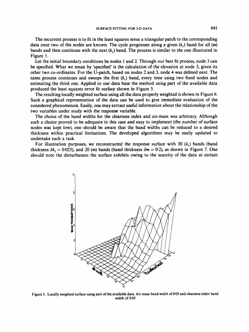
Let the initial boundary conditions be nodes 1 and 2. Through our best fit process, node 3 can be specified. What we mean by ‘specified’ is the calculation of the elevation at node 3, given its other two co-ordinates. For the U-patch, based on nodes 2 and 3, node 4 was defined next. The same process continues and sweeps the first (k,) band, every time using two fixed nodes and estimating the third one. Applied to our data base the method using part of the available data produced the least squares error fit surface shown in Figure 5.

The resulting locally weighted surface using all the data properly weighted is shown in Figure 6. Such a graphical representation of the data can be used to give immediate evaluation of the considered phenomenon. Easily, one may extract useful information about the relationship of the two variables under study with the response variable.

The choice of the band widths for the clearness index and air-mass was arbitrary. Although such a choice proved to be adequate in this case and easy to implement (the number of surface nodes was kept low), one should be aware that the band widths can be reduced to a desired thickness within practical limitations. The developed algorithms may be easily updated to undertake such a task.

For illustration purposes, we reconstructed the response surface with 30 ( k , ) bands (band thickness 6k, = 0-025), and 20 (m) bands (band thickness 6m = 0.2), as shown in Figure 7. One should note the disturbances the surface exhibits owing to the scarcity of the data at certain

i

Figure 5. Locally weighted surface using part of the available data. Air-mass band width of OO5 and clearness index band width of 005

642

1 c A. n A w u s AND s. M. JETER

Figure 6. Locally weightal surface using all the available data Air-mass band width of 1 and clcaroess index band width of 0 0 5

Figure 7. Locally weightedsurfaa wing d he. aMilablcdaip Air-masstand width of02 anddcarnersiadclbaod width of 0025

SURFACE FITTING FOR 3-D DATA 643

regions. In particular, a spurious data point in conjunction with the small working spaces of this example may result in an indeterminate case. Neighbouring patches with no data would be directly affected by such an anomaly. This is illustrated in Figure 7 along the last air-mass band and at high clearness indices. A total of 858 nodes is now required to fully describe the surface between the intervals of 1 < m < 5 and 0.1 < k, < 0.9 (the remaining nodes are on the k,-m plane). Owing to its high complexity, such a model may have low applicability for solar radiation modelling.

The user's specific needs and data quality would dictate the necessary accuracy. One, though, must be aware that the presence of erroneous data in the population combined with extremely narrow band widths may result in a highly disturbed surface, with numerous peaks and valleys. However, this adverse situation can be reversed to the advantage of the user. The sudden peaks, for example, can be used to identify questionable data that may have escaped previous data quality controls. Appropriate action may then be taken.

The two additional approaches using the surface fitting capabilities of IMSL and DISSPLA were also implemented with the available data. IMSL6 generated the response surface illustrated in Figure 8. One should use this method with sufficiently large working spaces to avoid excessive noise on the surface. We chose to use air-mass bands of unity (for the range of 1 < m < 5 ) and clearness index bands of 0.05 each, with a total of 8077 data. DISSPLA' generated Figure 9. A total of 8077 data was used by DISSPLA, between 1 < m c 5 with air-mass band thickness of unity and clearness index bands of 005.

6. CONCLUSIONS

The performance of the two approaches, using part of or all available data, for generating the response surfaces for the empirical data we have considered, and their relative performance against the response surfaces from IMSL and DISSPLA, may be determined with a number of statistical tests. The coefficient of determination (r') is often used to judge the adequacy of a regression model. The proposed method, using all the data properly weighted, produced

Figure 8. Surface generated by IMSL6 using all the available data. Air-mass band width of 1 and clearness index band width of 0.05

644 C. A. BALARAS A N D S. M. JETER

Figure 9. Surface generated by DISSPLA' using all the available data. Air-mass band width of 1 and clearness index band width of 0.05

a response surface with the best fit to the available data, and resulted in a coefficient of determination equal to 98.24 per cent. The method of using part of the data produced an ( r2) of 97.09 per cent. The fit, according to the coefficient of determination values, was slightly better in the case when all the data were used. In fact, this is the procedure we are proposing for future use.

In comparison to the alternative surface fitting methods, our approach produced superior results. DISSPLA produced a response surface for the available data with a coefficient of determination value equal to 95.54 per cent. According to our calculations, IMSL exhibited the poorest performance with a value of r2 equal to 92.25 per cent. An additional disadvantage of the IMSL method was the long execution time and large memory requirements that make its implementation for large numbers of data problematic.

We have previously presented several surfaces generated with different band thicknesses for the available data base. Their complexity was not justified by a substantial increase in their predictive powers. For reference, consider that the surface developed for the implementation of the method in Section 5, with an air-mass band thickness of 6m = 0.5 and clearness index band thickness of Sk, = 0.05, resulted in an rz equal to 98.34 per cent. For Sm = 0.2 and Sk, = 0.025 a value of 98472 per cent was calculated for the coefficient of determination.

As one would expect, a more dense surface resulted in a slight improvement in the performance of the model as illustrated by the increase in the value of the coefficient of determination. The significance for an improvement of the order of half of a per cent on the value of r2 for the case of 6m = 0.2 and Sk, = 0.025 over the case of Sm = 1 and Sk, = 0.05 is not justified considering the increased complexity of such a model. One just needs to recall that the more dense surface requires 858 nodes, while the case of Sm = 1 and Sk, = 005 bands requires a total of 102 nodes.

The surface fitting technique we have developed and applied to the available data set has proved to be successful. The proposed method may be applied to any three-variable study in order to describe the variability of a dependent variable in terms of two independent variables. The method is easy to implement and it allows for fast manipulation in order to achieve the

SURFACE FITTING FOR 3-D DATA 645

desirable accuracy of the developed locally weighted continuous surface to a three dimensional scattered data set. These features make this technique an attractive tool and it should be considered by researchers for similar studies.

ACKNOWLEDGEMENT

This work was conducted under the funding of the Georgia Power Company as part of the Solar Total Energy Project, Shenandoah, Georgia. The authors gratefully acknowledge the interest and encouragement of Mr E. J. Ney, Manager of Solar Operation for the Georgia Power Company.

REFERENCES

1. P. Lancaster and K. Salkauskas, Curue and Surface Fir-itting, Academic Press, London, 1986. 2. G. Farin, ‘Triangular Bernstein-Bezier patches’, Comp. Aided Geometric Des., 3, 83-127 (1986). 3. S. W. Sloan, ‘A fast algorithm for constructing Delaunay triangulations in the plane’, Adu. Eng. Software, 9, 34-55

4. Y. Correc and E. Chapuis, ‘Fast computation of Delaunay triangulations’, Adu. Eng. Software, 9, 77-83 (1987). 5. R. E. Barnhill, ‘Representation and approximation of surfaces’, in J. R. Rice (ed.), Mathematical Software 111, Academic

6. IMSL Library, International Mathematical and Statistical Libraries, Inc., Houston, Texas, 1977. 7. H. Akima, ‘A method of bivariate interpolation and smooth surface fitting for irregularly distributed data points’, ACM

8. DISSPLA, Display Integrated Software System and Plotting Language, Integrated Software Systems Co., 1981. 9. J. Fox, Linear Statistical Models and Related Methods, Wiley, New York, 1984.

(1987).

Press, New York, 1977.

Trans. Math. Software, 4, 148-159 (1978).