Articleshttps://doi.org/10.1038/s41559-018-0717-x

1Wellcome Sanger Institute, Cambridge, UK. 2Zoological Institute, University of Basel, Basel, Switzerland. 3Department of Genetics, University of Cambridge, Cambridge, UK. 4Department of Biology, University of Antwerp, Antwerp, Belgium. 5Naturalis Biodiversity Center, Leiden, The Netherlands. 6School of Natural Sciences, Bangor University, Bangor, UK. 7Gurdon Institute, University of Cambridge, Cambridge, UK. 8School of Biological Sciences, University of Bristol, Bristol, UK. 9Present address: Max Planck Institute for Biology of Ageing, Cologne, Germany. 10These authors contributed equally: Milan Malinsky, Hannes Svardal. *e-mail: millanek@gmail.com; rd109@cam.ac.uk

The formation of every lake or island represents a fresh oppor-tunity for colonization, proliferation and diversification of living forms. In some cases, the ecological opportunities pre-

sented by underutilized habitats facilitate adaptive radiation—rapid and extensive diversification of the descendants of the colonizing lineages1–3. Adaptive radiations are thus exquisite examples of the power of natural selection, as seen for example in Darwin’s finches in the Galapagos4,5, the Anolis lizards of the Caribbean6 and in East African cichlid fishes7,8.

Cichlids are one of the most species-rich and diverse families of vertebrates, and nowhere are their radiations more spectacular than in the Great Lakes of East Africa: lakes Malawi, Tanganyika and Victoria2, each of which contains several hundred endemic species, with the largest number in Lake Malawi9. Molecular genetic studies have made major contributions to reconstructing the evolutionary histories of these adaptive radiations, especially in terms of the rela-tionships between the lakes10,11, between some major lineages in Lake Tanganyika12, and in describing the role of hybridization in the ori-gins of the Lake Victoria radiation13. However, the task of reconstruct-ing within-lake relationships remains challenging owing both to the retention of large amounts of ancestral genetic polymorphism (that is, incomplete lineage sorting) and the gene flow between taxa12,14–18.

Initial genome assemblies of cichlids from East Africa suggest that an increased rate of gene duplication, together with accelerated evolution of some regulatory elements and protein coding genes, may have contributed to the radiations11. However, our understand-ing of the genomic mechanisms contributing to adaptive radiations is still in its infancy3.

Here we provide an overview of and insights into the genomic signatures of the haplochromine cichlid radiation of Lake Malawi.

The species that comprise the radiation can be divided into seven groups with differing ecology and morphology (see Supplementary Note): (1) the rock-dwelling ‘mbuna’; (2) Rhamphochromis—typi-cally midwater pelagic piscivores; (3) Diplotaxodon—typically deep-water pelagic zooplanktivores and piscivores; (4) deep-water and twilight-feeding benthic species; (5) ‘utaka’ feeding on zooplankton in the water column but breeding on or near the lake bottom (here utaka corresponds to the genus Copadichromis); (6) a diverse group of benthic species, mainly found in shallow non-rocky habitats; and (7) Astatotilapia calliptera, a closely related generalist that inhabits shallow weedy margins of Lake Malawi, and other lakes and rivers in the catchment, as well as river systems to the east and south of the Lake Malawi catchment. This division into seven groups has been partially supported by previous molecular phylogenies based on mitochondrial DNA (mtDNA) and amplified fragment length poly-morphism data18–20. However, published phylogenies show numer-ous inconsistencies and, in particular, the question of whether the groups are genetically separate remained unanswered.

To characterize the genetic diversity, species relationships, and sig-natures of selection across the whole radiation, we obtained Illumina whole-genome sequence data from 134 individuals of 73 species distributed broadly across the seven groups (Fig. 1a; Supplementary Note). This includes 102 individuals at ~15× coverage and 32 addi-tional individuals at ~6× coverage (Supplementary Table 1).

ResultsLow genetic diversity and species divergence. Sequence data were aligned to and variants called against a Metriaclima zebra refer-ence genome11. Average divergence from the reference was 0.19% to 0.27% (Supplementary Fig. 1). After filtering and variant refine-

Whole-genome sequences of Malawi cichlids reveal multiple radiations interconnected by gene flowMilan Malinsky   1,2,10*, Hannes Svardal   1,3,4,5,10, Alexandra M. Tyers6,9, Eric A. Miska   1,3,7, Martin J. Genner8, George F. Turner6 and Richard Durbin   1,3*

The hundreds of cichlid fish species in Lake Malawi constitute the most extensive recent vertebrate adaptive radiation. Here we characterize its genomic diversity by sequencing 134 individuals covering 73 species across all major lineages. The aver-age sequence divergence between species pairs is only 0.1–0.25%. These divergence values overlap diversity within species, with 82% of heterozygosity shared between species. Phylogenetic analyses suggest that diversification initially proceeded by serial branching from a generalist Astatotilapia-like ancestor. However, no single species tree adequately represents all species relationships, with evidence for substantial gene flow at multiple times. Common signatures of selection on visual and oxygen transport genes shared by distantly related deep-water species point to both adaptive introgression and independent selec-tion. These findings enhance our understanding of genomic processes underlying rapid species diversification, and provide a platform for future genetic analysis of the Malawi radiation.

NATuRE EcoloGy & EvoluTioN | VOL 2 | DECEMBER 2018 | 1940–1955 | www.nature.com/natecolevol1940

ArticlesNaTure eCoLogy & evoLuTioN

ment, we obtained 30.6 million variants, of which 27.1 million were single nucleotide polymorphisms (SNPs) and the rest were short insertions and deletions. All the following analyses are based on biallelic SNPs.

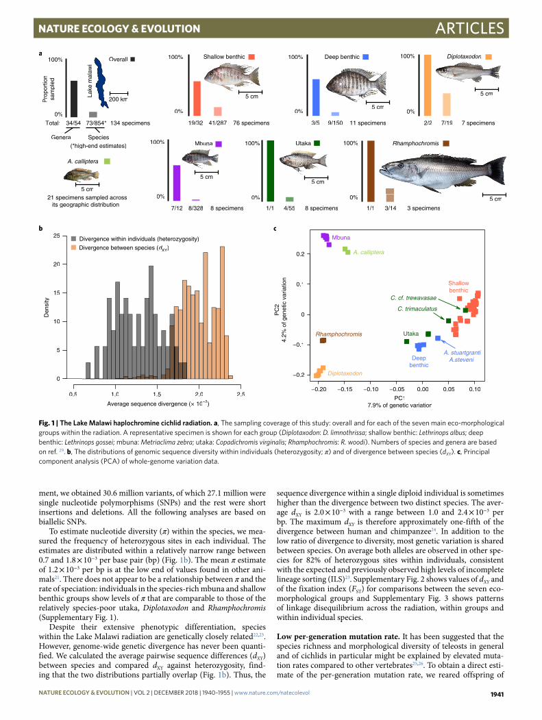
To estimate nucleotide diversity (π) within the species, we mea-sured the frequency of heterozygous sites in each individual. The estimates are distributed within a relatively narrow range between 0.7 and 1.8 × 10−3 per base pair (bp) (Fig. 1b). The mean π estimate of 1.2 × 10−3 per bp is at the low end of values found in other ani-mals21. There does not appear to be a relationship between π and the rate of speciation: individuals in the species-rich mbuna and shallow benthic groups show levels of π that are comparable to those of the relatively species-poor utaka, Diplotaxodon and Rhamphochromis (Supplementary Fig. 1).

Despite their extensive phenotypic differentiation, species within the Lake Malawi radiation are genetically closely related22,23. However, genome-wide genetic divergence has never been quanti-fied. We calculated the average pairwise sequence differences (dXY) between species and compared dXY against heterozygosity, find-ing that the two distributions partially overlap (Fig. 1b). Thus, the

sequence divergence within a single diploid individual is sometimes higher than the divergence between two distinct species. The aver-age dXY is 2.0 × 10−3 with a range between 1.0 and 2.4 × 10−3 per bp. The maximum dXY is therefore approximately one-fifth of the divergence between human and chimpanzee24. In addition to the low ratio of divergence to diversity, most genetic variation is shared between species. On average both alleles are observed in other spe-cies for 82% of heterozygous sites within individuals, consistent with the expected and previously observed high levels of incomplete lineage sorting (ILS)23. Supplementary Fig. 2 shows values of dXY and of the fixation index (FST) for comparisons between the seven eco-morphological groups and Supplementary Fig. 3 shows patterns of linkage disequilibrium across the radiation, within groups and within individual species.

Low per-generation mutation rate. It has been suggested that the species richness and morphological diversity of teleosts in general and of cichlids in particular might be explained by elevated muta-tion rates compared to other vertebrates25,26. To obtain a direct esti-mate of the per-generation mutation rate, we reared offspring of

0

5

10

15

20

25 Divergence within individuals (heterozygosity)

Divergence between species (dXYdd )

Average sequence divergence (× 10–3)

Den

sity

Diplotaxodon

0%

100%

2/2 7/19

Mbuna

0%

100% Rhamphochromis

0%

100%

1/1 3/14

Utaka

0%

100%

1/1 4/55

A. calliptera

21 specimens sampled acrossits geographic distribution

a

b c

0%

100%

73/854*34/54Total:

Pro

port

ion

sam

pled

Genera Species(*high-end estimates)

134 specimens

5 cm

5 cm5 cm

5 cm

Deep benthic

0%

100%

11 specimens 7 specimens3/5 9/150

5 cm5 cm

Shallow benthic

0%

100%

76 specimens

8 specimens8 specimens 3 specimens

19/32

7/12 8/328

41/287

5 cm

5 cm

Lake

mal

awi

200 km

Overall

−0.20 −0.15 −0.10 −0.050.5 1.0 1.5 2.0 2.5

0.00 0.05 0.10

−0.2

−0.1

0

0.1

0.2

PC

24.

2% o

f gen

etic

var

iatio

n

PC17.9% of genetic variation

A. calliptera

Mbuna

Rhamphochromis

Diplotaxodon

Utaka

Deepbenthic

Shallowbenthic

C. trimaculatus

A. stuartgrantiA.steveni

C. cf. trewavasae

Fig. 1 | The lake Malawi haplochromine cichlid radiation. a, The sampling coverage of this study: overall and for each of the seven main eco-morphological groups within the radiation. A representative specimen is shown for each group (Diplotaxodon: D. limnothrissa; shallow benthic: Lethrinops albus; deep benthic: Lethrinops gossei; mbuna: Metriaclima zebra; utaka: Copadichromis virginalis; Rhamphochromis: R. woodi). Numbers of species and genera are based on ref. 29. b, The distributions of genomic sequence diversity within individuals (heterozygosity; π) and of divergence between species (dXY). c, Principal component analysis (PCA) of whole-genome variation data.

NATuRE EcoloGy & EvoluTioN | VOL 2 | DECEMBER 2018 | 1940–1955 | www.nature.com/natecolevol 1941

Articles NaTure eCoLogy & evoLuTioN

three species from three different Lake Malawi groups (A. calliptera, Aulonocara stuartgranti and Lethrinops lethrinus). We sequenced both parents and one offspring of each to high coverage (40× ), applied stringent quality filtering, and counted variants present in each offspring but absent in both its parents (Supplementary Fig. 4). There was no evidence for significant difference in mutation rates between species. The overall mutation rate (μ) was estimated at 3.5 × 10−9 (95% confidence interval (CI): 1.6 × 10−9 to 4.6 × 10−9) per bp per generation, approximately three to four times lower than in humans27, although, given much shorter mean generation times, the per-year rate is still expected to be higher in cichlids than in humans. We note that ref. 26 obtained a much higher mutation rate estimate (6.6 × 10−8 per bp per generation) in Midas cichlids, but from relatively low-depth sequencing of restriction-site-associated markers that may have made accurate verification more difficult. We also note that our per-generation rate estimate, although low, is still higher than the lowest μ estimate in vertebrates: 2 × 10−9 per bp per generation recently reported for Atlantic herring28. By combining our mutation rate with nucleotide diversity (π) values, we estimate the long term effective population sizes (Ne) to be in the range of approximately 50,000 to 130,000 breeding individuals (with Ne = π/4μ).

Genome data support for eco-morphological groupings. PCA of the whole-genome genotype data generally separates the major eco-morphological groups (Fig. 1c). The most notable exceptions to this are (1) the utaka, for which some species cluster more closely with deep benthics and others with shallow benthics, and (2) two spe-cies of the genus Aulonacara, A. stuartgranti and A. steveni, which are located between the shallow and deep benthic groups. Although these have enlarged lateral-line sensory apparatus like many deep benthic species including other Aulonocara, they are typically found in shallower water29. Another interesting pattern in the PCA plot is that the utaka and benthic samples are often spread along prin-cipal component (PC) axes (Fig. 1c, Supplementary Fig. 5), a pat-tern typical for admixed populations (for example ref. 30). Along the two main PCs, the deeper-water benthic species extend towards the deep-water Diplotaxodon, an observation we will return to in the context of gene flow and shared mechanisms of depth adaptation.

To further verify the consistency of group assignments, we tested whether pairs of species from the same group always share more derived alleles with each other than with any species from other groups. Group assignments were again supported, except for the four species also highlighted in the PCA: the two shallow-living Aulonocara are closer to shallow benthics than to deep benthics in 71% and 82% of tests respectively when comparing these alterna-tives, and Copadichromis trimaculatus is closer to shallow benthics than to utaka in 58% of the comparisons. Copadichromis cf. trewava-sae always clustered with shallow benthics; therefore, we treat it as a member of the shallow benthic group henceforth. With the three intermediate samples removed and C. cf. trewavasae reassigned, all other species showed 100% consistency with their group assignment.

Allele sharing inconsistent with tree-like relationships. The above observations suggest that some species may be genetically intermediate between well defined groups, consistent with previ-ous studies that have suggested that hybridization and introgression subsequent to initial separation of species may have played a signifi-cant part in cichlid radiations, including in lakes Tanganyika12,14–16 and Malawi18,20. Where this happens, there is no single tree relating the species.

To assess the overall extent of violation of tree-like species rela-tionships, we calculated Patterson’s D statistic (the ABBA-BABA test)31,32 for all possible trios of Lake Malawi species, without assum-ing any a priori knowledge of their relationships. N. brichardi from Lake Tanganyika was always used as the outgroup. The test statistic

Dmin is the minimum absolute value of Patterson’s D for each trio, across all possible tree topologies. Therefore, a significantly positive Dmin score signifies that the sharing of derived alleles between the three species is inconsistent with a single species tree relating them, even in the presence of incomplete lineage sorting.

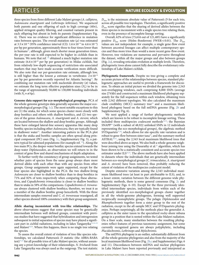
Overall, 62% of trios (75,616 out of 121,485) have a significantly positive Dmin score (Holm–Bonferroni FWER < 0.01). The Dmin values are not independent: for example, a single gene-flow event between ancestral lineages can affect multiple contemporary spe-cies and thus more trios than would a more recent gene-flow event. However, tree violations are numerous and pervasive throughout the dataset, within all the major groups and also between groups (Fig. 2a), revealing reticulate evolution at multiple levels. Therefore, phylogenetic trees alone cannot fully describe the evolutionary rela-tionships of Lake Malawi cichlids.

Phylogenetic framework. Despite no tree giving a complete and accurate picture of the relationships between species, standard phy-logenetic approaches are useful to provide a framework for discus-sion. To obtain an initial picture we divided the genome into 2,543 non-overlapping windows, each comprising 8,000 SNPs (average size 274 kb) and constructed a maximum likelihood phylogeny sep-arately for the full sequences within each window, obtaining trees with 2,542 different topologies. We also calculated the maximum clade credibility (MCC) summary tree33 and a maximum likeli-hood phylogeny based on the full mtDNA genome (Fig. 2b and Supplementary Fig. 6).

We next applied a range of further phylogenomic methods which are known to be robust to incomplete lineage sorting. These included three multispecies coalescent methods34,35: the Bayesian SNAPP36 (with a subset of 48,922 unlinked SNPs in 12 individuals representing the eco-morphological groups), the algebraic method SVDquartets37,38, which allows for site-specific rate variation and is robust to gene-flow between sister taxa39, and the summary method ASTRAL40,41, using the 2,543 local maximum likelihood trees that were described above as input. We also built a whole-genome neigh-bour-joining tree using the Dasarathy et al.42 algorithm, which has been shown to be a statistically consistent and accurate species tree estimator under ILS42,43. The above methods have also been applied to datasets where the individuals that are genetically intermediate between eco-morphological groups (C. trimaculatus, A. stuartgranti and A. steveni) have been removed, thus probably reducing the extent of violation of the multispecies coalescent model.

Despite extensive variation among the 2,543 individual maxi-mum likelihood trees (at least in part attributable to ILS), and, to a lesser extent, variation between the different genome-wide phy-logenetic methods, there is some general consensus (Fig. 2c and Supplementary Figs. 6–10). Except for the three previously iden-tified intermediate species, individuals from within each of the previously identified eco-morphological groups cluster together in all the whole-genome phylogenies, forming well supported reciprocally monophyletic groups. The pelagic Diplotaxodon and Rhamphochromis together form a sister group to the rest of the radiation, except in the all-sample MCC and SVDquartets phylog-enies. Perhaps surprisingly, all the methods place the generalist A. calliptera as the sister taxon to the specialized rocky-shore mbuna group in a position that is nested within the Lake Malawi radiation. On a finer scale, many similarities between the resulting phylog-enies reflect features of previous taxonomic assignment, but some currently recognized genera are always polyphyletic, including Placidochromis, Lethrinops and Mylochromis.

The mtDNA phylogeny is an outlier, substantially different from all the whole-genome phylogenies and also from the majority of the local maximum likelihood trees (Fig. 2b,c and Supplementary Figs. 6 and 11). Discordances between mtDNA and nuclear phylogenies in Lake Malawi have been reported previously and interpreted as

NATuRE EcoloGy & EvoluTioN | VOL 2 | DECEMBER 2018 | 1940–1955 | www.nature.com/natecolevol1942

ArticlesNaTure eCoLogy & evoLuTioN

a signature of past hybridization events18,20. However, as we discuss below, some of these previously suggested hybridization events are not reflected in the whole-genome data. Indeed, large discrepan-cies between mitochondrial and nuclear phylogenies have been shown in many other systems, reflecting both that mtDNA as a single locus is not expected to reflect the consensus under ILS, and high incidence of mitochondrial selection44–46. This underlines the

importance of evaluating species relationships in the Lake Malawi radiation from a genome-wide perspective.

Specific signals of introgression. We applied a variety of meth-ods to identify the species and groups whose relationships violate the framework trees described in the previous section. First, we contrasted the pairwise genetic distances used to produce the

a

c

b

200 40 60 80 100

Proportion of trios (%)

0 5 10 15 20Dmin (%)

2 group comparisons

3 group comparisons

mtDNA tree

Lake Massoko

Salima, Malawi

Copadichromisvirginalis

Aulonocarastuartgranti

Lethrinopsalbus

Otopharynxspeciosus

Dimidiochromisstrigatus

R. woodi

D. limnothrissa

Mbu

naS

hallo

wbe

nthi

c

Dee

pbe

nthi

c

Utaka

Diplotaxodon

Rhamphochromis

Within mbuna

Within A. calliptera

Within shallow benthic

Within deep benthic

Within Diplotaxodon

SVDQ

NJ

SNAPP.t2

NJ*

SNAPP.t1

ASTRAL

MCC

ASTRAL*

MCC

SVDQ*

0 20 40 60 80 100

SVDQNJ

SNAPP.t2NJ*

SNAPP.t1

ASTRALM

CC

ASTRAL*M

CC

SVDQ*

Mai

n tr

ees

12 s

ampl

etr

ees

Method

Sup.Fig. 9

Sup.Fig. 9

Sup.Fig. 6

Sup.Fig. 6

Sup.Fig. 8

Sup.Fig. 8

Sup.Fig. 5a

Sup.Fig. 5b

Sup.Fig. 7

Sup.Fig. 7

Fig. 2b

Meandistance

Normalized Robinson–Foulds pairwise treedistance (%)

mtDNARAxML

mtD

NA

RAxML

* trees that exclude samples withintermediate group assignment:C. trimaculatus, A. steveni and A. stuartgranti

31.0

30.9

30.6

25.3

38.3

32.8

50.5

83.9

18.2

17.7

25.0

9

30

15

41

37

57

89

0

22

10

28

21

36

38

54

88

11

12

12

13

34

32

48

89

0

22

10

34

33

49

88

0

0

0

6

57

90

25

38

22

53

89

14

14

12

91

22

44

30

67

78

70

17

0 20

*

*

**

*

*

*

N. brichardi

A. c

allip

tera

Lethrinopsgossei

Iodotropheussprengarae

Metriaclimazebra

Maximum clade credibility tree

Clades supported by ≥ 50% of trees

Fig. 2 | Excess allele sharing and patterns of species relatedness. a, Derived allele sharing reveals non-tree-like relationships among trios of species. The bars show the proportion of significantly elevated Dmin scores (see main text). Shading corresponds to FWER q values of (from light to dark) 10−2, 10−4, 10−8 and 10−14. The scatterplots show the Dmin scores that were significant with family-wise error rate (FWER) <  0.01. Results are shown separately for comparisons where all three species in the trio are from the same group, and for cases where the species come from two or three different groups. Rhamphochromis and utaka within-group comparisons are not shown owing to the low number of data points. b, A set of 2,543 maximum likelihood phylogenetic trees for non-overlapping regions along the genome. Branch lengths were scaled for visualization so that the total height of each tree is the same. The local trees were built with 71 species and then subsampled for display to 12 individuals representing the eco-morphological groups. The maximum clade credibility tree shown here was built from the subsampled local trees. A maximum likelihood mitochondrial phylogeny is shown for comparison. c, A summary of all phylogenies from this study and the normalized Robinson–Foulds distances between them, reflecting the topological distance between pairs of trees on the scale from zero to 100%. The least-controversial 12-sample tree is SNAPP.t1, with an average distance to other trees of 17.7%, while ASTRAL* is the least controversial among the ‘main trees’ (mean distance of 25.3%). To compare trees with differing sets of taxa, the trees were downsampled so that only matching taxa were present. The position of the outgroup/root was considered in all comparisons. Supplementary figures associated with the phylogenies are indicated for each tree.

NATuRE EcoloGy & EvoluTioN | VOL 2 | DECEMBER 2018 | 1940–1955 | www.nature.com/natecolevol 1943

Articles NaTure eCoLogy & evoLuTioN

neighbour-joining tree against the distances between samples along the tree branches, calculating the residuals (Supplementary Fig. 12). If the tree captured all the genetic relationships in our sample per-fectly, the residuals would all be zero. However, as expected in light of the Dmin analysis above, we found numerous differences, affecting both groups of species and individual species, with some standout cases. Among the strongest signals on individual species, in addi-tion to the previously discussed C. trimaculatus, we can see that (1) Placidochromis cf. longimanus is genetically closer to the deep ben-thic clade and to a subset of the shallow benthic (mainly Lethrinops species) than the tree suggests; and (2) our sample of Otopharynx tetrastigma (from Lake Ilamba) is much closer to A. calliptera (espe-cially to the sample from Lake Kingiri, only 3.2 km away) than is expected from the tree.

Second, the sharing of long haplotypes between otherwise dis-tantly related species is an indication of recent admixture or intro-gression. To investigate this type of gene flow signature, we used the chromopainter software package47 and calculated the ‘co-ancestry matrix’ of all species—a summary of nearest-neighbour (therefore recent) haplotype relationships. The Lake Ilamba O. tetrastigma and Lake Kingiri A. calliptera also stand out in this analysis, showing a strong signature of recent gene flow between individual species from distinct eco-morphological groups (Supplementary Fig. 13). The other tree-violation signatures described above are also visible on the haplotype sharing level but are less pronounced, consistent with being older events involving the common ancestors of multiple present-day species. However, the chromopainter results indicate additional recent introgression events (for example, the utaka C. virginalis with Diplotaxodon; more highlighted in Supplementary Fig. 13). Furthermore, the clustering based on recent co-ancestry is different from all phylogenetic trees: in particular a number of shallow benthics, including P. cf. longimanus, cluster next to the deep benthics.

Third, we used the f4 admixture ratio31,32,48 (f statistic; closely related to Patterson’s D), computing f(A,B;C,O) for all groups of species that fit the relationships ((A, B), C) in the ASTRAL* tree (Supplementary Fig. 7), with the outgroup fixed as N. brichardi. When elevated owing to introgression, the f statistic is expected to be linear in relation to the proportion of introgressed material. The ASTRAL* tree has the lowest mean topological distance to all the other trees, and excludes the three species with intermediate group assignment, a choice made here because we were interested in iden-tifying additional signals beyond the admixed status of A. stuart-granti, A. steveni and C. trimaculatus. Out of the 164,320 computed f statistics, 97,889 were significant at FWER < 0.001.

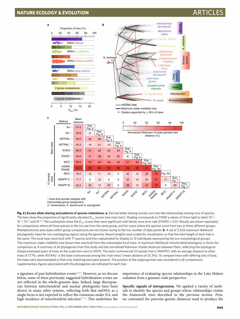
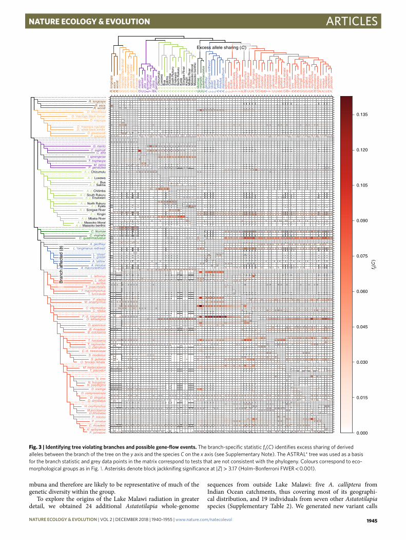
As in the case of Dmin, a single gene-flow event can lead to multiple significant f statistics. Noting that the values for different combina-tions of ((A, B), C) groups are not independent as soon as they share branches on the tree, we sought to obtain branch-specific estimates of excess allele sharing that would be less correlated. Building on the logic employed to understand correlated gene flow signals in ref. 49, we developed the ‘f-branch’ metric or fb(C): a summary of f scores that, on a given tree, captures excess allele sharing between a species C and a branch b compared to the sister branch of b (Methods). Therefore, an fb(C) score is specific to the branch b (on the y-axis in Fig. 3), but a single introgression event can still lead to significant fb(C) values across multiple related C values. There were 11,158 fb(C) scores of which 1,421 were significantly elevated at FWER < 0.001 (Supplementary Fig. 14), and 238 scores were larger than 3% (the value inferred for human–Neanderthal introgression in ref. 31). The majority of nodes in the tree are affected: 92 of the 158 branches in the phylogeny show significant excess allele sharing with at least one other species C (Fig. 3).

Overall, the highest fb(C) (14.2%) is between the ancestor of the two sampled Ctenopharynx species from the shallow benthic group and the utaka Copadichromis virginalis (Fig. 3). Notably,

Ctenopharynx species, particularly C. intermedius and C. pictus, have very large numbers of long slender gill rakers, a feature shared with Copadichromis species, and believed to be related to a diet of small invertebrates50. Several other benthic lineages also share excess alleles with C. virginalis, however these signals are less pronounced. Next, the significantly elevated fb(C) scores between the shallow and the deep benthic lineages suggest that genetic exchanges between these two groups go beyond the clearly admixed shallow-living Aulonacara (not included in this analysis). The f-branch signals between O. tetrastigma and A. calliptera Kingiri are observed in both directions—A. calliptera Kingiri with shallow benthics (and most strongly O. tetrastigma) and O. tetrastigma with A. calliptera (most strongly A. calliptera Kingiri), suggesting bi-directional introgression.

At the level of the major eco-morphological groups, the stron-gest signal indicates that the ancestral lineage of benthics and utaka shares excess derived alleles with Diplotaxodon and, to a lesser degree, Rhamphochromis, as previously suggested by the PCA plot (Fig. 1c). Furthermore, there is evidence for addi-tional ancestry from the pelagic groups in utaka, which could be explained either by an additional, more recent, gene-flow event or by differential fixation of introgressed material, possibly due to selection. Reciprocally, Diplotaxodon shares excess derived alleles (relative to Rhamphochromis) with utaka and deep benthics, as does Rhamphochromis with mbuna and A. calliptera. Furthermore, mbuna show excess allele sharing (relative to A. calliptera) with Diplotaxodon and Rhamphochromis (Fig. 3). On the other hand, while ref. 18 suggested gene flow between the deep benthic and mbuna groups on the basis of a discrepancy between mtDNA and nuclear phylogenies, our genome-wide analysis did not find any sig-nal of substantial genetic exchange between these groups.

The f statistic tests are robust to the occurrence of incomplete lin-eage sorting, in the sense that ILS alone cannot generate a significant test result32. We note, however, that pronounced population structure within ancestral species, coupled with rapid succession of speciation events, can also substantially violate the assumptions of a strictly bifurcating species tree and lead to significantly elevated f scores32,51. This needs to be taken into account when interpreting non-tree-like relationships, for example among major groups early in the radiation. However, in cases of excess allele sharing between ‘distant’ lineages that are separated by multiple speciation events, ancestral population structure would have needed to segregate through these speciation events without affecting sister lineages, a scenario that is not cred-ible in general. Therefore, we suggest that there is strong evidence for multiple cross-species gene flow events. Additionally, simulations suggest that, compared with treemix52, fb(C) is robust to misspecifica-tion of the initial tree (Supplementary Note).

Overall, the neighbour-joining tree residuals, the haplotype sharing patterns and the many elevated fb(C) scores paint a consis-tent picture. They confirm the extensive violations of the bifurcating species tree model initially revealed by the Dmin analysis, and suggest many independent gene-flow events at different times during the evolutionary history of the adaptive radiation.

Origins of the radiation. The generalist Astatotilapia calliptera has been referred to as the ‘prototype’ for the endemic Lake Malawi cich-lids29,53, and discussions concerning the origin of the radiation often centre on ascertaining its relationship to the Malawi species20,54. Previous phylogenetic analyses, using mtDNA and small numbers of nuclear markers, showed inconsistencies in this respect18,20,54. In contrast, our whole-genome data indicated a clear and consistent position of the Lake Malawi catchment A. calliptera as a sister group to the mbuna, in agreement with the nuclear DNA phylogeny in a previous study18. While it is not certain whether the 320 remaining mbuna species form a monophyletic group with the eight species we used here, the eight species represent the majority of the genera of

NATuRE EcoloGy & EvoluTioN | VOL 2 | DECEMBER 2018 | 1940–1955 | www.nature.com/natecolevol1944

ArticlesNaTure eCoLogy & evoLuTioN

mbuna and therefore are likely to be representative of much of the genetic diversity within the group.

To explore the origins of the Lake Malawi radiation in greater detail, we obtained 24 additional Astatotilapia whole-genome

sequences from outside Lake Malawi: five A. calliptera from Indian Ocean catchments, thus covering most of its geographi-cal distribution, and 19 individuals from seven other Astatotilapia species (Supplementary Table 2). We generated new variant calls

A. c

. Mas

soko

ben

thic

A. c

. Chi

zum

ulu

C. likomae

A. geoffreyi

0.000

0.015

0.030

0.045

0.060

0.075

0.090

0.105

0.120

0.135

P. johnstoni

Bra

nch

affe

cted

(b)

f b(C

)

Excess allele sharing (C )

H. spilopterus

P. ornatusP. milomo

C. rhoadesii

O.lithobatesM.ericotaenia

H. oxyrhynchus

D. dimidiatusD. strigatus

D. compressicepsD. kiwinge

N. livingstoniN. polystigma

N. linni

T. placodonM. melanotaenia

O. 'brooksi nkhata'S. guttatus

S. modestusC. cf. trewavasae

C. caeruleusT. nigriventerT. holotaenia

B. nototaeniaB. rhoadesii

O. speciosus

O. tetrastigmaP. cf. longimanus

C. nitidusC. intermedius

M. anaphyrmusP. electra

T. furcicaudaT. macrorhynchus

T. praeorbitalisL. auritus

L. albusL. lethrinus

A. macrocleithrumA. minutusA. 'yellow'

L. 'oliveri' L. gossei

L. 'longimanus redhead'

C. quadrimaculatusC. virginalis

A. c. Massoko benthicA. c. Massoko littoral

A. c. Mbaka RiverA. c. Kingiri

A. c. Songwe RiverA. c. Kyela

A. c. North Rukuru

A. c. EnukweniA. c. South Rukuru

A. c. Chitimba

A. c. SalimaA. c. Bua

A. c. Luwawa

A. c. ChizumuluP. genalutea

M. zebraT. tropheopsI. sprengerae

C. afraC. axelrodi

G. mento

P. tokoloshD. greenwodi

D. 'white back similis'D. 'macrops ngulube'

D. macropsD. 'macrops black dorsal'

D. limnotrissaR. woodiR. esox

R. longiceps

R. l

ongi

ceps

R. w

oodi

R. e

sox

P.to

kolo

shD

. gre

enw

odi

D. '

whi

te b

ack

sim

ilis'

D. '

mac

rops

ngu

lube

'D

. mac

rops

D. '

mac

rops

bla

ck d

orsa

l'D

. lim

notr

issa

P.g

enal

utea

M. z

ebra

T. t

roph

eops

I. sp

reng

erae

C. a

fra

C. a

xelro

diG

. men

to

A. c

. Mas

soko

litto

ral

A. c

. Mba

ka R

iver

A. c

. Kin

giri

A. c

. Kye

laA

. c. N

orth

Ruk

uru

A. c

. Enu

kwen

iA

. c. S

outh

Ruk

uru

A. c

. Chi

timba

A. c

. Sal

ima

A. c

. Bua

A. c

. Luw

awa

A. c

. Son

gwe

Riv

er

C. l

ikom

ae

C. q

uadr

imac

ulat

usC

. virg

inal

is

A. g

eoffr

eyi

A. m

acro

clei

thru

mA

. min

utus

A. '

yello

w'

L. 'o

liver

i'L.

gos

sei

L. 'l

ongi

man

us r

edhe

ad'

T. n

igriv

ente

rT

. hol

otae

nia

B. n

otot

aeni

aB

. rho

ades

iiO

. spe

cios

usO

. tet

rast

igm

aP

. cf.

long

iman

usC

. niti

dus

C. i

nter

med

ius

M. a

naph

yrm

usP

. ele

ctra

T. f

urci

caud

aT

. mac

rorh

ynch

usT

. pra

eorb

italis

L. a

uritu

sL.

alb

usL.

leth

rinus

O. '

broo

ksi n

khat

a'S

. gut

tatu

sS

. mod

estu

sC

. cf.

trew

avas

aeC

. cae

rule

us

P. j

ohns

toni

H. s

pilo

pter

us

P. o

rnat

usP

. milo

mo

C. r

hoad

esii

O.li

thob

ates

M.e

ricot

aeni

aH

. oxy

rhyn

chus

D. d

imid

iatu

sD

. str

igat

usD

. com

pres

sice

psD

. kiw

inge

N. l

ivin

gsto

niN

. pol

ystig

ma

N. l

inni

T. p

laco

don

M. m

elan

otae

nia

Fig. 3 | identifying tree violating branches and possible gene-flow events. The branch-specific statistic fb(C) identifies excess sharing of derived alleles between the branch of the tree on the y axis and the species C on the x axis (see Supplementary Note). The ASTRAL* tree was used as a basis for the branch statistic and grey data points in the matrix correspond to tests that are not consistent with the phylogeny. Colours correspond to eco-morphological groups as in Fig. 1. Asterisks denote block jackknifing significance at |Z| > 3.17 (Holm–Bonferroni FWER <  0.001).

NATuRE EcoloGy & EvoluTioN | VOL 2 | DECEMBER 2018 | 1940–1955 | www.nature.com/natecolevol 1945

Articles NaTure eCoLogy & evoLuTioN

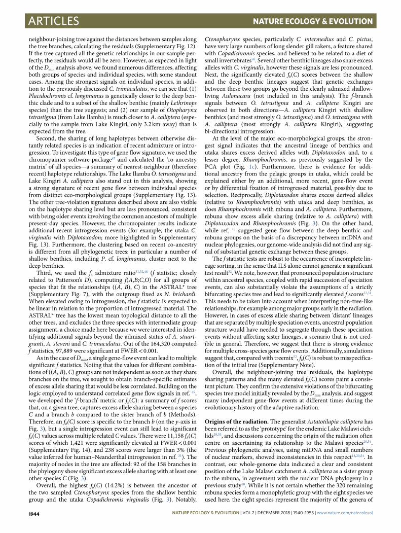
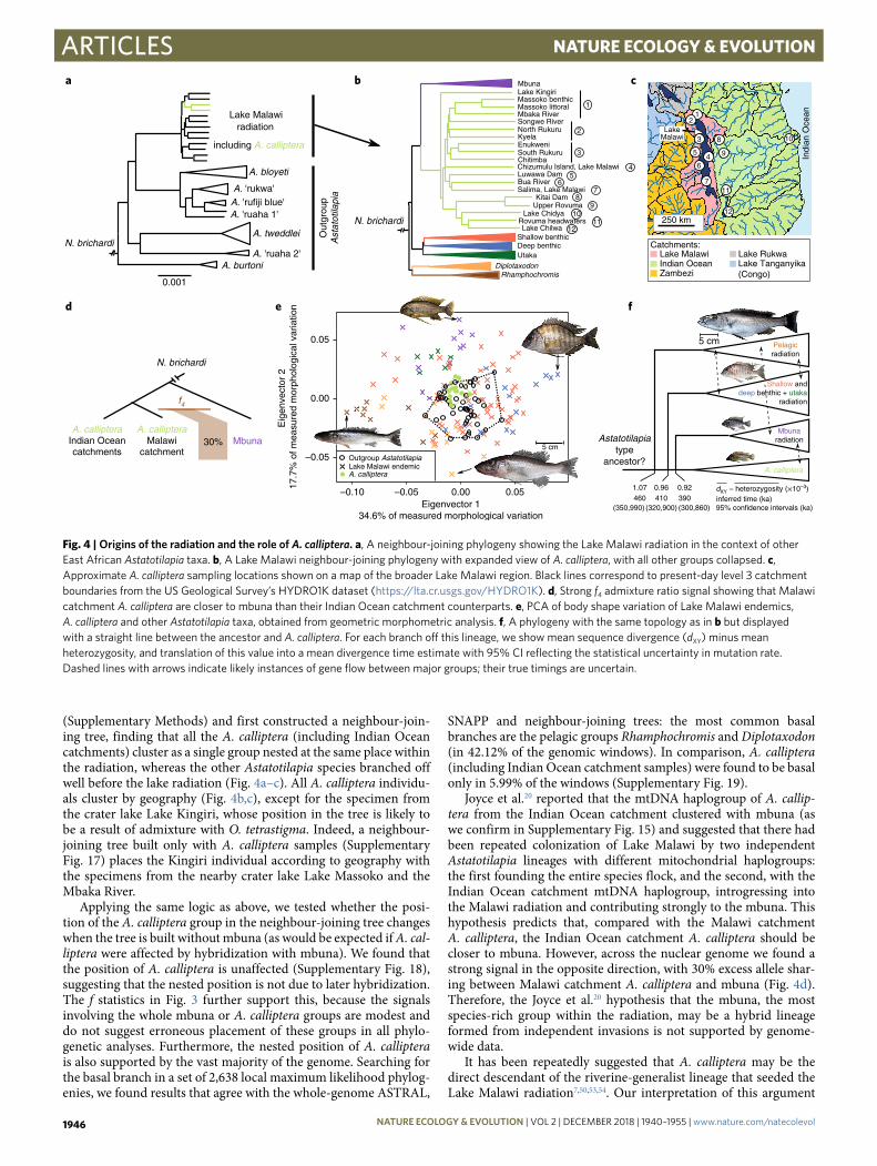
(Supplementary Methods) and first constructed a neighbour-join-ing tree, finding that all the A. calliptera (including Indian Ocean catchments) cluster as a single group nested at the same place within the radiation, whereas the other Astatotilapia species branched off well before the lake radiation (Fig. 4a–c). All A. calliptera individu-als cluster by geography (Fig. 4b,c), except for the specimen from the crater lake Lake Kingiri, whose position in the tree is likely to be a result of admixture with O. tetrastigma. Indeed, a neighbour-joining tree built only with A. calliptera samples (Supplementary Fig. 17) places the Kingiri individual according to geography with the specimens from the nearby crater lake Lake Massoko and the Mbaka River.

Applying the same logic as above, we tested whether the posi-tion of the A. calliptera group in the neighbour-joining tree changes when the tree is built without mbuna (as would be expected if A. cal-liptera were affected by hybridization with mbuna). We found that the position of A. calliptera is unaffected (Supplementary Fig. 18), suggesting that the nested position is not due to later hybridization. The f statistics in Fig. 3 further support this, because the signals involving the whole mbuna or A. calliptera groups are modest and do not suggest erroneous placement of these groups in all phylo-genetic analyses. Furthermore, the nested position of A. calliptera is also supported by the vast majority of the genome. Searching for the basal branch in a set of 2,638 local maximum likelihood phylog-enies, we found results that agree with the whole-genome ASTRAL,

SNAPP and neighbour-joining trees: the most common basal branches are the pelagic groups Rhamphochromis and Diplotaxodon (in 42.12% of the genomic windows). In comparison, A. calliptera (including Indian Ocean catchment samples) were found to be basal only in 5.99% of the windows (Supplementary Fig. 19).

Joyce et al.20 reported that the mtDNA haplogroup of A. callip-tera from the Indian Ocean catchment clustered with mbuna (as we confirm in Supplementary Fig. 15) and suggested that there had been repeated colonization of Lake Malawi by two independent Astatotilapia lineages with different mitochondrial haplogroups: the first founding the entire species flock, and the second, with the Indian Ocean catchment mtDNA haplogroup, introgressing into the Malawi radiation and contributing strongly to the mbuna. This hypothesis predicts that, compared with the Malawi catchment A. calliptera, the Indian Ocean catchment A. calliptera should be closer to mbuna. However, across the nuclear genome we found a strong signal in the opposite direction, with 30% excess allele shar-ing between Malawi catchment A. calliptera and mbuna (Fig. 4d). Therefore, the Joyce et al.20 hypothesis that the mbuna, the most species-rich group within the radiation, may be a hybrid lineage formed from independent invasions is not supported by genome-wide data.

It has been repeatedly suggested that A. calliptera may be the direct descendant of the riverine-generalist lineage that seeded the Lake Malawi radiation7,50,53,54. Our interpretation of this argument

d

1

10

11

8

2

3

5

6

7

4

12

9

Catchments:Lake MalawiIndian OceanZambezi

Shallow benthicDeep benthicUtaka

DiplotaxodonRhamphochromis

Lake RukwaLake Tanganyika(Congo)

N. brichardi

b

f

Astatotilapiatype

ancestor?

5 cm Pelagicradiation

Shallow anddeep benthic + utaka

radiation

Mbunaradiation

A. calliptera

1.07 0.96 0.92390

dXY − heterozygosity (×10–3)inferred time (ka)460

(350,990)410

(320,900) (300,860) 95% confidence intervals (ka)

c

A. tweddlei

A. bloyeti

A. 'rukwa'

Lake Malawiradiation

A. burtoni

including A. calliptera

A. 'rufiji blue'

A. 'ruaha 2'

A. 'ruaha 1'

Out

grou

pA

stat

otila

pia

a

e

N. brichardi

0.001

Eigenvector 134.6% of measured morphological variation

Eig

enve

ctor

2

17.7

% o

f mea

sure

d m

orph

olog

ical

var

iatio

n

0.00–0.05–0.10

Mbuna

Massoko benthicMassoko littoralMbaka River

1

Songwe RiverNorth RukuruKyela

2

EnukweniSouth RukuruChitimba

3

Chizumulu Island, Lake Malawi

Salima, Lake MalawiBua RiverLuwawa Dam

Lake ChilwaRovuma headwaters

Lake Chidya

Kitai DamUpper Rovuma

Lake Kingiri

4

76

1211

10

89

5

0.00

0.05

–0.05

A. calliptera

Outgroup AstatotilapiaLake Malawi endemic

N. brichardi

f4

Mbuna30%A. calliptera

Malawicatchment

A. callipteraIndian Oceancatchments

LakeMalawi

250 km

Indi

an O

cean

0.05

5 cm

Fig. 4 | origins of the radiation and the role of A. calliptera. a, A neighbour-joining phylogeny showing the Lake Malawi radiation in the context of other East African Astatotilapia taxa. b, A Lake Malawi neighbour-joining phylogeny with expanded view of A. calliptera, with all other groups collapsed. c, Approximate A. calliptera sampling locations shown on a map of the broader Lake Malawi region. Black lines correspond to present-day level 3 catchment boundaries from the US Geological Survey’s HYDRO1K dataset (https://lta.cr.usgs.gov/HYDRO1K). d, Strong f4 admixture ratio signal showing that Malawi catchment A. calliptera are closer to mbuna than their Indian Ocean catchment counterparts. e, PCA of body shape variation of Lake Malawi endemics, A. calliptera and other Astatotilapia taxa, obtained from geometric morphometric analysis. f, A phylogeny with the same topology as in b but displayed with a straight line between the ancestor and A. calliptera. For each branch off this lineage, we show mean sequence divergence (dXY) minus mean heterozygosity, and translation of this value into a mean divergence time estimate with 95% CI reflecting the statistical uncertainty in mutation rate. Dashed lines with arrows indicate likely instances of gene flow between major groups; their true timings are uncertain.

NATuRE EcoloGy & EvoluTioN | VOL 2 | DECEMBER 2018 | 1940–1955 | www.nature.com/natecolevol1946

ArticlesNaTure eCoLogy & evoLuTioN

is that the ancestor was probably a riverine generalist that was ecologically and phenotypically similar to A. calliptera and other Astatotilapia. This hypothesis is lent further support by geometric morphometric analysis. Using 17 homologous body shape land-marks we established that, despite the relatively large genetic diver-gence, A. calliptera is nested within the morphospace of the other more distantly related but ecologically similar Astatotilapia spe-cies (Fig. 4a,e), and these together have a central position within the morphological space of the Lake Malawi radiation (Fig. 4e and Supplementary Fig. 16).

To reconcile the nested phylogenetic position of A. calliptera with its generalist ‘prototype’ phenotype, we propose a model where the Lake Malawi species flock consists of three separate radiations splitting off from the lineage leading to A. calliptera. The relation-ships between the major groups supported by the ASTRAL, SNAPP and neighbour-joining methods suggest that the pelagic radiation was seeded first, then the benthic + utaka, and finally the rock-dwelling mbuna, all in a relatively quick succession, followed by subsequent gene flow as described above (Fig. 4f; the pelagic versus utaka + benthic branching order is swapped in the SVDquartets tree in Supplementary Fig. 9). Applying our per-generation mutation rate to observed genomic divergences we obtained mean divergence time estimates between these lineages between 460 thousand years ago (ka) (95% CI 350–990 ka) and 390 ka (95% CI 300–860 ka) (Fig. 4f), assuming three years per generation as in ref. 55. The point estimates all fall within the second-most recent prolonged deep-lake phase inferred from the Lake Malawi paleoecological record56, while the upper ends of the confidence intervals cover the third deep-lake phase at about 800 ka. Considering that our split time estimates from sequence divergence are likely to be reduced by subsequent gene-flow, leading to underestimates, the data are consistent with a previous report based on fossil time calibration which put the origin of the Lake Malawi radiation at 700–800 ka12.

The fact that the common ancestor of all the A. calliptera appears to be younger than the Malawi radiation suggests that the Lake Malawi A. calliptera population has been a reservoir that has repop-ulated the river systems and more transient lakes following dry–wet transitions in the East African hydroclimate56,57. Our results do not fully resolve whether the lineage leading from the common ancestor to A. calliptera retained its riverine generalist phenotype throughout or whether a lacustrine species evolved at some point (for example, the common ancestor of A. calliptera and mbuna) and later de-spe-cialized again to recolonize the rivers. However, while it is a possi-bility, we suggest that it is unlikely that the many strong phenotypic affinities of A. calliptera to the basal Astatotilapia (Fig. 4e; refs 58,59) would be reinvented from a lacustrine species.

Signatures and consequences of selection on coding sequences. To gain insight into the functional basis of diversification and adaptation in Lake Malawi cichlids, we next turned our attention to protein-coding genes. We compared the mean between-species levels of non-synonymous variation pN

to synonymous variation pS

in 20,664 genes and calculated the difference between these two val-ues ( δ = −− p pN S N S

). Overall, coding sequence exhibits signatures of purifying selection: the average between-species pN

was 54% lower than in a random matching set of non-coding regions. Interestingly, the average between-species synonymous variation pS

in genes was 13% higher than in non-coding control regions ( < . × −P 2 2 10 16, one-tailed Mann–Whitney U-test). One possible explanation of this observation would be if intergenic regions were homogenized by gene flow, whereas protein-coding genes were more resistant to this.

To control for statistical effects of variation in gene length and sequence composition we normalized the δN−S values per gene by taking into account the variance across all pairwise sequence com-parisons for each gene, deriving the non-synonymous excess score ΔN−S (see Methods). Values at the upper tail of the distribution of

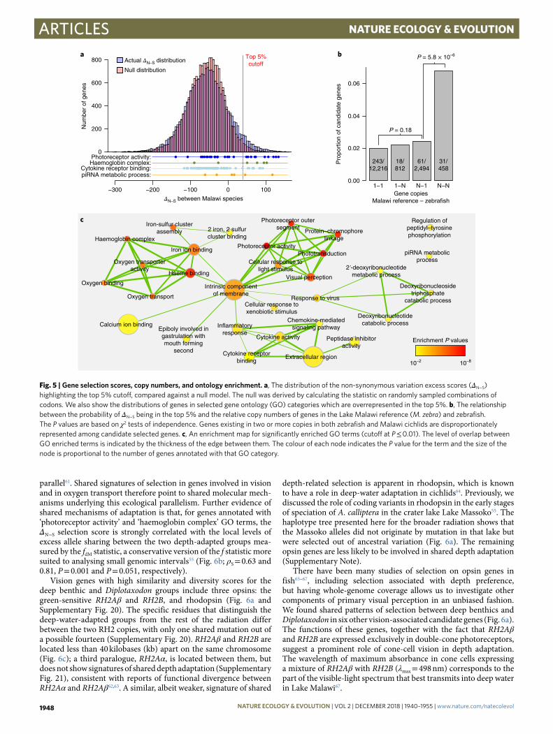
ΔN−S are substantially over-represented in the actual data when com-pared to a null model based on random sampling of codons (Fig. 5a). We focus below on the top 5% of the distribution (ΔN−S > 40.2, 1034 candidate genes). Genes with elevated ΔN−S are expected to have been under positive selection at multiple non-synonymous sites, either recently repeatedly within multiple species or ances-trally. Therefore, the statistic reveals only a limited subset of posi-tive selection events from the history of the radiation (for example a selection event on a single amino acid would not be detected). Furthermore, to minimize any effect of gene prediction errors, all the following analyses focus on the 15,980 (77.3% of total) genes for which zebrafish homologues were found in a previous study11; selection scores of genes without homologues are briefly discussed in the Supplementary Note.

Cichlids have an unexpectedly large number of gene duplicates, which has possibly contributed to their extensive adaptive radia-tions3,11. To investigate the extent of divergent selection on gene duplicates, we examined how the ΔN−S scores are related to gene copy numbers in the reference genomes. Focusing on homologous genes annotated both in the Malawi reference (M. zebra) and in the zebrafish genome, we found that the highest proportion of candidate genes was among genes with two or more copies in both genomes (N − N). The relative enrichment in this category is both substantial and highly significant (Fig. 5b). On the other hand, the increase in proportion of candidate genes in the N − 1 category (multiple cop-ies in the M. zebra genome but only one copy in zebrafish) is much smaller and is not significant (χ2 test P = 0.18), suggesting that selec-tion is occurring more often within ancient multi-copy gene fami-lies, rather than on genes with cichlid-specific duplications.

We used GO annotation of zebrafish homologues to test whether candidate genes are enriched for particular functional categories (Methods). We found significant enrichment for 30 GO terms (range: 1.6 × 10−8 < P < 0.01, weigh algorithm60; Supplementary Table 3): 10 in the ‘molecular function’, 4 in the ‘cellular component’ and 16 in the ‘biological process’ category. Combining all the results in a network (connecting terms that share many genes) revealed clear clusters of enriched terms related to (1) haemoglobin function and oxygen transport; (2) phototransduction and visual perception; and (3) the immune system, especially inflammatory response and cytokine activity (Fig. 5c). That evolution of genes in these func-tional categories has contributed to cichlid radiations has been sug-gested previously (see below); it is nevertheless interesting that these categories stand out in a genome-wide analysis.

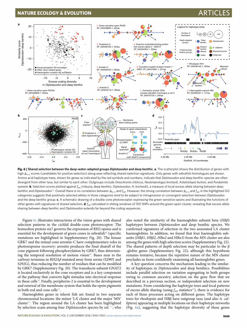
Shared mechanisms of depth adaptation. To gain insight into the distribution of adaptive alleles across the radiation, we built maximum likelihood trees from amino acid sequences of candidate genes, thus summarizing potentially complex haplotype genealogy networks. Focusing on the significantly enriched GO categories, many haplotype trees have features that are unusual in the broader dataset: the haplotypes from the deep benthic group and the deep-water pelagic Diplotaxodon tend to group together (despite these two groups being distant in whole-genome phylogenies and mono-phyletic in only two out of 2,638 local maximum likelihood trees) and also tend to be disproportionally diverse when compared with the rest of the radiation. We quantified both excess similarity and diversity, and found that both measures are elevated for candidate genes in the ‘visual perception’ category (Fig. 6a; Mann–Whitney U-tests: P = 0.007 for similarity, P = 0.08 for shared diversity, and P = 0.003 when the scores are added) and also for the ‘haemoglo-bin complex’ category (P values not significant owing to the small number of genes).

Sharply decreasing levels of dissolved oxygen and low light intensities with narrow short-wavelength spectra are the hallmarks of the habitats below about 50 m to which the deep benthic and Diplotaxodon groups have both adapted, either convergently or in

NATuRE EcoloGy & EvoluTioN | VOL 2 | DECEMBER 2018 | 1940–1955 | www.nature.com/natecolevol 1947

Articles NaTure eCoLogy & evoLuTioN

parallel61. Shared signatures of selection in genes involved in vision and in oxygen transport therefore point to shared molecular mech-anisms underlying this ecological parallelism. Further evidence of shared mechanisms of adaptation is that, for genes annotated with ‘photoreceptor activity’ and ‘haemoglobin complex’ GO terms, the ΔN−S selection score is strongly correlated with the local levels of excess allele sharing between the two depth-adapted groups mea-sured by the fdM statistic, a conservative version of the f statistic more suited to analysing small genomic intervals55 (Fig. 6b; ρS = 0.63 and 0.81, P = 0.001 and P = 0.051, respectively).

Vision genes with high similarity and diversity scores for the deep benthic and Diplotaxodon groups include three opsins: the green-sensitive RH2Aβ and RH2B, and rhodopsin (Fig. 6a and Supplementary Fig. 20). The specific residues that distinguish the deep-water-adapted groups from the rest of the radiation differ between the two RH2 copies, with only one shared mutation out of a possible fourteen (Supplementary Fig. 20). RH2Aβ and RH2B are located less than 40 kilobases (kb) apart on the same chromosome (Fig. 6c); a third paralogue, RH2Aα, is located between them, but does not show signatures of shared depth adaptation (Supplementary Fig. 21), consistent with reports of functional divergence between RH2Aα and RH2Aβ62,63. A similar, albeit weaker, signature of shared

depth-related selection is apparent in rhodopsin, which is known to have a role in deep-water adaptation in cichlids64. Previously, we discussed the role of coding variants in rhodopsin in the early stages of speciation of A. calliptera in the crater lake Lake Massoko55. The haplotype tree presented here for the broader radiation shows that the Massoko alleles did not originate by mutation in that lake but were selected out of ancestral variation (Fig. 6a). The remaining opsin genes are less likely to be involved in shared depth adaptation (Supplementary Note).

There have been many studies of selection on opsin genes in fish65–67, including selection associated with depth preference, but having whole-genome coverage allows us to investigate other components of primary visual perception in an unbiased fashion. We found shared patterns of selection between deep benthics and Diplotaxodon in six other vision-associated candidate genes (Fig. 6a). The functions of these genes, together with the fact that RH2Aβ and RH2B are expressed exclusively in double-cone photoreceptors, suggest a prominent role of cone-cell vision in depth adaptation. The wavelength of maximum absorbance in cone cells expressing a mixture of RH2Aβ with RH2B (λmax = 498 nm) corresponds to the part of the visible-light spectrum that best transmits into deep water in Lake Malawi67.

1−1 1−N N−1 N−N

Photoreceptor activity:Haemoglobin complex:

Cytokine receptor binding:piRNA metabolic process:

ΔN–S between Malawi species

Num

ber

of g

enes

Top 5%cutoff

Gene copiesMalawi reference – zebrafish

Pro

port

ion

of c

andi

date

gen

es

a b

0.06

0.04

0.02

0.00

P = 0.18

P = 5.8 × 10–6

243/12,216

18/812

61/2,494

31/458

0

800

600

400

200

−300 −200 −100 1000

Iron ion binding

Oxygen binding

Iron-sulfur clusterassembly

Haemoglobin complex

Oxygen transport

Calcium ion binding

Oxygen transporteractivity

Epiboly involved ingastrulation withmouth forming

second

Haeme binding

2 iron, 2 sulfurcluster binding

Cellular response tolight stimulus

Phototransduction

Regulation ofpeptidyl–tyrosinephosphorylation

Photoreceptor activity

Photoreceptor outersegment

Protein–chromophorelinkage

piRNA metabolicprocess

Inflammatoryresponse

Deoxyribonucleotidecatabolic process

Peptidase inhibitoractivity

Cytokine activity

Extracellular region

Chemokine-mediatedsignaling pathway

Cytokine receptorbinding

Intrinsic componentof membrane

2ʹ-deoxyribonucleotidemetabolic process

Response to virus

Visual perception

Cellular response toxenobiotic stimulus

Deoxyribonucleosidetriphosphate

catabolic process

Enrichment P values

10–2 10–8

c

Actual ΔN–S distribution

Null distribution

Fig. 5 | Gene selection scores, copy numbers, and ontology enrichment. a, The distribution of the non-synonymous variation excess scores (ΔN−S) highlighting the top 5% cutoff, compared against a null model. The null was derived by calculating the statistic on randomly sampled combinations of codons. We also show the distributions of genes in selected gene ontology (GO) categories which are overrepresented in the top 5%. b, The relationship between the probability of ΔN−S being in the top 5% and the relative copy numbers of genes in the Lake Malawi reference (M. zebra) and zebrafish. The P values are based on χ2 tests of independence. Genes existing in two or more copies in both zebrafish and Malawi cichlids are disproportionately represented among candidate selected genes. c, An enrichment map for significantly enriched GO terms (cutoff at P ≤  0.01). The level of overlap between GO enriched terms is indicated by the thickness of the edge between them. The colour of each node indicates the P value for the term and the size of the node is proportional to the number of genes annotated with that GO category.

NATuRE EcoloGy & EvoluTioN | VOL 2 | DECEMBER 2018 | 1940–1955 | www.nature.com/natecolevol1948

ArticlesNaTure eCoLogy & evoLuTioN

Figure 6c illustrates interactions of the vision genes with shared selection patterns in the cichlid double-cone photoreceptor. The homeobox protein six7 governs the expression of RH2 opsins and is essential for the development of green cones in zebrafish68 (specific mutations are highlighted in Supplementary Fig. 20). The kinase GRK7 and the retinal cone arrestin-C have complementary roles in photoresponse recovery: arrestin produces the final shutoff of the cone pigment following phosphorylation by GRK7, thus determin-ing the temporal resolution of motion vision69. Bases near to the carboxy terminus in RH2Aβ mutated away from serine (S290Y and S292G), thus reducing the number of residues that can be modified by GRK7 (Supplementary Fig. 20). The transducin subunit GNAT2 is located exclusively in the cone receptors and is a key component of the pathway that converts light stimulus into electrical response in these cells70. Finally, peripherin-2 is essential to the development and renewal of the membrane system that holds the opsin pigments in both rod and cone cells71.

Haemoglobin genes in teleost fish are found in two separate chromosomal locations: the minor ‘LA’ cluster and the major ‘MN’ cluster72. The region around the LA cluster has been highlighted by selection scans among four Diplotaxodon species by ref. 73, who

also noted the similarity of the haemoglobin subunit beta (HBβ) haplotypes between Diplotaxodon and deep benthic species. We confirmed signatures of selection in the two annotated LA cluster haemoglobins. In addition, we found that four haemoglobin sub-units (HBβ1, HBβ2, HBα2 and HBα3) from the MN cluster are also among the genes with high selection scores (Supplementary Fig. 22). The shared patterns of depth selection may be particular to the β -globin genes (Supplementary Fig. 22), although this hypothesis remains tentative, because the repetitive nature of the MN cluster precludes us from confidently examining all haemoglobin genes.

A key question concerns the mechanism leading to the similar-ity of haplotypes in Diplotaxodon and deep benthics. Possibilities include parallel selection on variation segregating in both groups owing to common ancestry, selection on the gene flow that we described in a previous section, or independent selection on new mutations. From considering the haplotype trees and local patterns of excess allele sharing (using fdM statistics55), there is evidence for each of these processes acting on different genes. The haplotype trees for rhodopsin and HBβ have outgroup taxa (and also A. cal-liptera) appearing at multiple locations on their haplotype networks (Fig. 6a), suggesting that the haplotype diversity of these genes

Nucleus (opsin transcription

via six7 homologue)?

Outersegment

Six7 Six7

RH2B

Phosphorylatedby GRK7

Membranedisks holding opsins

PP

Signalquenched

PP

PP

Transcducin(with GNAT2 component)

PP

PP

PP

PP

PP

PP

PP

P

Arrestin-C

PP

Peripherin-2(disk regeneration)

Detail of opsin interactions:

b d

Scaffold_18 coordinates

4.30 Mb 4.35 Mb 4.40 Mbf dM

0.6

0.4

0.2

0.0

–0.2 Assembly gaps:Accessiblegenome:

RH2BRH2Aβ RH2Aα

Geneannotation:

5: Arrestin-CXP_004550345.1; 355aa

4: Guanine nucleotide-binding proteinG(t) subunit alpha-2 - GNAT2XP_004554304.1; 350aa

2: Green-sensitive opsin RH2BXP_004548806.1; 352aa

1: Green-sensitive opsin RH2AβXP_004548809.1; 352aa

6: G-protein-coupled receptor kinase 7 -GRK7 XP_004570581.1; 557aa

a: Arrestin-CXP_004545716.1; 365aa

3: Peripherin-2XP_004556729.1; 343aa

A: Haemoglobin subunit HBβXP_004562337.1; 147aa

−10 −5 0 5 10

−20

−10

0

10

20 2

Visual perception GO annotation

13

Other vision related genes

7

Excess coding diversityin Diplotaxodon and deep benthic

Sim

ilarit

y sc

ore

Dip

lota

xodo

n–de

ep b

enth

ic

56

b: Homeobox protein SIX6(closest zebrafish homologue is six7 )XP_004570733.1; 260aa

7: Rhodopsin RH1XP_004546142.1; 354aa

1

Massokolittoral

Massokobenthic

b4

a

a

c

Photoreceptor activity GO

fdM

Haemoglobin complex GO

Δ N–S

A

Haemoglobin complex GO annotation

–200

–400

0

200

–0.8 –0.4 0.0 0.4 0.8

RH2B

Number ofhaplotypes:

Depth adaptedgroups:

10 20 40 1001

Deepbenthic

Diplotaxodon

Predominantlyshallow groups: Mbuna Rhamphochomis

Shallowbenthic

A. calliptera

Utaka Outgroups

Legend for haplotype trees:

T

RH2Aβ

Fig. 6 | Shared selection between the deep-water-adapted groups Diplotaxodon and deep benthic. a, The scatterplot shows the distribution of genes with high ΔN−S scores (candidates for positive selection) along axes reflecting shared selection signatures. Only genes with zebrafish homologues are shown. Amino acid haplotype trees, shown for genes as indicated by the red symbols and numbers, indicate that Diplotaxodon and deep benthic species are often divergent from other taxa, but similar to each other. Outgroups include Oreochromis niloticus, Neolamprologus brichardi, Astatotilapia burtoni, and Pundamilia nyererei. b, Selection scores plotted against fdM (mbuna, deep benthic; Diplotaxodon, N. brichardi), a measure of local excess allele sharing between deep benthic and Diplotaxodon55. Overall there is no correlation between Δ N−S and fdM. However, the strong correlation between ΔN−S and fdM in the highlighted GO categories suggests that positively selected alleles in those categories tend to be subject to introgression or convergent selection between Diplotaxodon and the deep benthic group. c, A schematic drawing of a double cone photoreceptor expressing the green-sensitive opsins and illustrating the functions of other genes with signatures of shared selection. d, fdM calculated in sliding windows of 100 SNPs around the green opsin cluster, revealing that excess allele sharing between deep benthic and Diplotaxodon extends far beyond the coding sequences.

NATuRE EcoloGy & EvoluTioN | VOL 2 | DECEMBER 2018 | 1940–1955 | www.nature.com/natecolevol 1949

Articles NaTure eCoLogy & evoLuTioN

may reflect ancestral variation. In contrast, trees for the green cone genes show the Malawi radiation all being derived with respect to outgroups and we found substantially elevated fdM scores extending for around 40 kb around the RH2 cluster (Fig. 6d), consistent with adaptive introgression in a pattern reminiscent of mimicry loci in Heliconius butterflies74. Finally, the peaks in fdM around peripherin-2 and one of the arrestin-C genes are narrow, ending at the gene boundaries, and fdM scores are elevated only for non-synonymous variants; synonymous variants do not show excess allele sharing (Supplementary Fig. 23). Owing to the close proximity of non-syn-onymous and synonymous sites within the same gene, this suggests that for these two genes there may have been independent selection on the same de novo mutations.

DiscussionVariation in genome sequences forms the substrate for evolution. Here we described genome variation at the full sequence level across the Lake Malawi haplochromine cichlid radiation. We focused on ecomorphological diversity, representing more than half the genera from each major group, rather than obtaining deep coverage of spe-cies within any particular group. Therefore, we have more samples from the morphologically highly diverse benthic lineages than, for example, from the mbuna where there are relatively fewer genera and many species are largely recognized by colour differences.

The observation that cichlids within an African Great Lake radi-ation are genetically very similar is not new75, but we now quantify the relationship of this to within-species variation, and the conse-quences for variation in local phylogeny across the genome. The fact that between-species divergence is generally only slightly higher than within species diversity, is probably the result of the young age of the radiation, the relatively low mutation rate and of gene flow between taxa. Within-species diversity itself is relatively low for vertebrates, at around 0.1%, suggesting that low genome-wide nucleotide diversity levels do not necessarily limit rapid adaptation and speciation, results that are in contrast to a recent report that found that high diversity levels may have been important for rapid adaptation in Atlantic killifish76. One possibility is that in cichlids repeated selection has maintained diversity in adaptive alleles for a range of traits that support ecological diversification, as we have concluded for rhodopsin and HBβ and as appears to be the case for some adaptive variants in sticklebacks77.

We provide evidence that gene flow during the radiation, although not ubiquitous, has certainly been extensive. Overall, the numerous violations of the bifurcating species tree model suggest that full resolution of interspecies relationships in this system will require network approaches (see for example section 6.2 of ref. 35) and population genomic analyses within the structured coales-cent framework with gene flow. The majority of the signals affect groups of species, suggesting events involving their common ances-tors, or are between closely related species within the major eco-logical groups. The only strong and clear example of recent gene flow between individual distantly related species is not within Lake Malawi itself, but between Otopharynx tetrastigma from crater Lake Ilamba and local A. calliptera. Lake Ilamba is very turbid and the scenario is reminiscent of cichlid admixture in low-visibility condi-tions in Lake Victoria78. It is possible that some of the earlier signals of gene flow between lineages we observed in Lake Malawi may have happened during periods of low lake level when the water is known to have been more turbid56.

Our model of the early stages of radiation in Lake Malawi (Fig. 4f) is broadly consistent with the model of initial separation by major habitat divergence23, although we propose a refinement in which there were three relatively closely spaced separations from a generalist Astatotilapia type lineage, initially of pelagic genera Rhamphochromis and Diplotaxodon, then of shallow- and deep-water benthics and utaka (this includes Kocher’s sand dwellers23,29),

and finally of mbuna. Thus, we suggest that Lake Malawi contains three separate haplochromine cichlid radiations stemming from the generalist lineage, interconnected by subsequent gene flow.

The finding that cichlid-specific gene duplicates do not tend to diverge particularly strongly in coding sequences (Fig. 5b) suggests that other mechanisms of diversification following gene duplica-tions may be more important. Divergence via changes in expression patterns has previously been illustrated and discussed11, and future studies addressing structural variation between cichlid genomes will assess the contribution of differential retention of duplicated genes.

The evidence concerning shared adaptation of the visual and oxygen-transport systems to deep-water environments between deep benthics and Diplotaxodon suggests different evolutionary mechanisms acting on different genes, even within the same cellular system. It will be interesting to see whether the same genes or even specific mutations underlie depth adaptation in Lake Tanganyika, which harbours specialist deep-water species in least two different tribes79 and has a similar light attenuation profile but a steeper oxy-gen gradient than Lake Malawi61.

Over the last few decades, East African cichlids have emerged as a model for studying rapid vertebrate evolution11,23. Taking advantage of recently assembled reference genomes11, our data and results pro-vide insight into patterns of sequence sharing and adaptation across the Lake Malawi radiation, and into mechanisms of rapid phenotypic diversification. The datasets are publicly available (see ‘Data avail-ability’) and will underpin further studies on specific taxa and molec-ular systems. For example, we envisage that our results, clarifying the relationships between all the main lineages and many individual species, will facilitate speciation studies, which require investigation of taxon pairs at varying stages on the speciation continuum80,81, and studies on the role of adaptive gene flow in speciation.

MethodsSamples. Ethanol-preserved fin clips were collected by M. J. Genner and G. F. Turner between 2004 and 2014 from Tanzania and Malawi, in collaboration with the Tanzania Fisheries Research Institute (the MolEcoFish Project) and with the Fisheries Research Unit of the Government of Malawi (various collaborative projects). Samples were collected and exported with the permission of the Tanzania Commission for Science and Technology, the Tanzania Fisheries Research Institute, and the Fisheries Research Unit of the Government of Malawi.

From sequencing to a variant callset. The analyses presented above are based on SNPs obtained from Illumina short (100–125 bp) reads, aligned to the M. zebra reference assembly version 1.111 with bwa-mem82, followed by GATK haplotype caller83 and samtools/bcftools84 variant calling restricted to 653 Mb of ‘accessible genome’ where variants can be determined confidently with short reads, filtering, genotype refinement, imputation and phasing in BEAGLE85 and further haplotype phasing with shapeit v286, including the use of phase-informative reads87. For details please see Supplementary Methods.

Linkage disequilibrium calculations. The haplotype disequilibrium coefficient88 r2 between pairs of SNPs was calculated along the phased scaffolds 0 to 201 (scaffolds are assembled fragments of the reference genome and scaffolds 0–201 are longer than 1 Mb), using vcftools v0.1.12b89 with the options --hap-r2 --ld-window-bp 50000. To reduce the computational burden, we used a random subsample of 10% of SNPs. We binned the r2 values according to the distance between SNPs into 1-kb or 100-bp windows and plotted the average values in each bin.

To estimate background linkage disequilibrium, we calculated haplotype r2 between variants mapping to different linkage groups in the Oreochromis niloticus genome assembly. First, we used the chain files generated by the whole genome alignment pipeline90 (see Supplementary Methods) and the UCSC liftOver tool (http://hgdownload.soe.ucsc.edu/downloads.html#source_downloads) to translate the genomic coordinates of all SNPs to the O. niloticus coordinates. Then we calculated linkage disequilibrium between variants mapping to linkage groups LG1 and LG2.

De novo mutation rate estimation. In each trio we looked for mutations in the child that were not present in either of its parents. Because the results of this analysis are very sensitive to false positives and false negative rates, we used higher coverage sequencing (about 40× average) and applied more stringent genome masks than in the population genomic work. Increased coverage supports clean separation of sequencing errors and somatic mutations from true heterozygous

NATuRE EcoloGy & EvoluTioN | VOL 2 | DECEMBER 2018 | 1940–1955 | www.nature.com/natecolevol1950

ArticlesNaTure eCoLogy & evoLuTioN

calls in the offspring, and improved ability to distinguish single copy versus multi-copy sequence on a per-individual basis.

First we determined the ‘accessible genome’ (that is the regions of the genome in which the mutations can be confidently called (de novo mutations) for each trio by excluding:

1. Genomic regions where mapped read depth in any member of a trio is ≤ 25× or > 50×

2. Bases where either of the parents has a mapped read that does not match the reference (the specific bases where any read has non-reference alleles in the parents were masked)

3. Sequences where indels (base insertion or deletion) were called in any sample (we also excluded ± 3 bp of sequence surrounding the indel)

4. Sites that were called as multiallelic among the nine samples in the overall trios dataset

5. Known segregating variable sites— that is, sites with alternative alleles found in four and more copies in the overall Lake Malawi dataset

6. Sites in the reference where less than 90% of overlapping 50-mers (sub-sequences of length 50) could be matched back uniquely and without 1-difference. For this we used Heng Li’s SNPable tool (http://lh3lh3.users.sourceforge.net/snpable.shtml), dividing the reference genome into overlapping k-mers (sequences of length k; we used k = 50), and then aligning the extracted k-mers back to the genome (we used bwa aln -R 1000000 -O 3 -E 3).

After excluding sites in the categories above, we were left with an ‘accessible genome’ of 516.6 Mb in the A. calliptera trio, 459 Mb in the A. stuartgranti trio and 404 Mb in the L. lethrinus trio. Because any observed de novo mutation could have occurred either on the chromosome inherited from the mother or on the chromosome inherited from the father, the point estimate of the per-generation per-base-pair mutation rate is: μ = nmutations/(2 × the size of the accessible genome).

Next we set out to search for de novo mutations: that is, heterozygous sites in the offspring within the accessible genome. Under random sampling there is an equal probability of seeing a read with either of the two alleles at a heterozygous site. Therefore, Na (the number of reads supporting the alternative allele) is distributed as approximately Binomial(read depth, 0.5). We filtered out variants with observed Na values below the 2.5th or above the 97.5th percentiles of this distribution, thus accepting a false-negative rate of 5%. We also filtered out sites where the offspring call had Read Position or Base Quality rank-sum test Z-score exceeding the 99.5th percentile of the standard normal distribution or where the strand-bias phred-scaled P value (− log10(error probablility)) was ≥ 20 or where the phred-scaled genotype quality in either mother, father or offspring was ≤ 30. For simplicity, assuming these filters are independent, they are expected to introduce a false-negative rate of 7.17%. The mutation rate estimate was adjusted to account for this.

After filtering, we found nine de novo mutations across the three offspring. For each mutation we double-checked the alignment in the IGV genome browser and found all of them were single base mutations supported by high number of reads (> 8) in the offspring. The 95% confidence intervals for the number of observed mutations were calculated using the ‘exact’ method relating γ2 and Poisson distributions91,92. If N is the number of observed mutations, the lower (ciNL) and upper (ciNU) limits are:

χ χ=

≤ .=

≥ .+P PciN

( 0 025)2

ciN( 0 975)

2N N

L22

U2( 1)2

where 2N and 2(N + 1) are the degrees of freedom of the corresponding γ2 distributions.

PCA. SNPs with minor allele frequency ≥ 0.05 were selected using the bcftools (v1.2) view option --min-af 0.05:minor. The program vcftools v0.1.12b was then used to export that data into PLINK format93. Next, the variants were linkage-disequilibrium-pruned to obtain a set of variants in approximate linkage equilibrium (unlinked sites) using the --indep-pairwise 50 5 0.2 option in PLINK v1.0.7. PCA on the resulting set of variants was performed using the smartpca program from the eigensoft v5.0.2 software package94 with default parameters.

Genome-wide FST calculations. In addition to performing PCA, the smartpca program from the eigensoft v5.0.2 software package also calculates genome-wide FST for all pairs of populations specified by the sixth column in the .pedind file. For the calculation, it uses the Hudson estimator, as defined previously95 in their equation (10), and the ‘ratio of averages’ is used to combine estimates of FST across multiple variants, as they recommended. We used all SNPs (no minor allele frequency filtering).

Allele sharing test for group assignment. We tested whether two individuals who come from the same group always share more derived alleles with each other than with any individuals from other groups. Technically, we implemented this using the D statistic (ABBA-BABA tests) framework31,32, by calculating D A G G O( , ; , )1 2 for all permutations of individuals, where G1 and G2 come from the same

eco-morphological group and A from a different group. The outgroup O was always N. brichardi from Lake Tanganyika. Note that this is an unusual use of the D statistics and our aim here was not to look for gene flow but to test whether allele sharing is greater within eco-morphological groups (G1 with G2) compared to across groups (A with G2), in which case >D A G G O( , ; , ) 01 2 . All results were statistically significant, which was assessed using block jackknife31 on windows of 60,000 SNPs.

Dmin statistic. Here we calculated the D statistic for each trio of species (A,B,C) and for all possible tree topologies (the outgroup again fixed as N. brichardi). Therefore, Dmin = min(|D(A,B;C,O)|, |D(A,C;B,O)|, |D(C,B;A,O)|. If this is significantly elevated, then allele sharing within the trio of species is inconsistent with any simple tree topology. Note that this approach is conservative in the sense that the Dmin score for each trio is considered in isolation and we ignore ‘higher-order’ inconsistencies where different Dmin trio topologies are inconsistent with each other. Statistical significance was assessed using block jackknife31 on windows of 60,000 SNPs and family wise error rate (FWER) was calculated following the Holm–Bonferroni method.

Sample selection for demographic analyses. To prevent potential confounding effects of uneven sequencing depth, we limited these analyses to one high-coverage (15× ) individual per species. Species without a high-coverage sample (P. subocularis, F. rostratus and L. trewavasae) were not included.

Outgroup sequences/alleles. Outgroup (Supplementary Table 5) sequences in M. zebra genomic coordinates were obtained based on pairwise whole-genome alignments (Supplementary Methods). Insertions in the outgroup were ignored and deletions filled by ‘N’ characters.

Local phylogenetic trees and maximum clade credibility. To generate a multiple alignment input in fasta format we used the getWGSeq subprogram of evo. We set the window size in terms of the numbers of variants rather than physical length (8,000 variants; the --split 8,000 option) aiming for the local regions to have similar strengths of phylogenetic signal. Small windows at the ends of scaffolds were discarded. We limited the sequence output to the accessible genome using the --accessibleGenomeBED option. The N. brichardi outgroup sequence in M. zebra genomic coordinates was added via the --incl-Pn option.

Maximum likelihood phylogenies were inferred using RAxML version 7.7.896 under the GTRGAMMA model. The best tree for each region was selected out of twenty alternative runs on distinct starting maximum parsimony trees (the -N 20 option).

The MCC trees were calculated in TreeAnnotator version 2.4.2, a part of the BEAST2 platform97. Clade credibility is the frequency with which a clade appears in the tree set; the MCC tree is the tree (from among the trees in the set) that maximizes the product of the frequencies of all its clades33. The node heights for the MCC trees are derived as a summary from the heights of each clade in the whole tree set via the ‘common ancestor’ heights option.

Mitochondrial DNA phylogenies. The mtDNA sequence corresponds to scaffolds 747 and 2,036 in the M. zebra reference. Variants from these scaffolds were subjected to the same filtering as in the rest of the genome except for the depth filter because the mapped read depth was much higher (approximately 300–400× per sample). Because of the greater sequence diversity in the mtDNA genome, we found that more than 10% of variants were multiallelic. Therefore, we separated SNPs from indels at multiallelic sites using bcftools norm with the --multiallelics - option, then removed indels and the merged multiallelic SNPs back together with the --multiallelics + option. Sequences in the fasta format were generated using the bcftools consensus command, and missing genotypes in the VCF replaced by the ‘N’ character with the --mask option. The N. brichardi outgroup sequence in M. zebra genomic coordinates was added to the fasta files.

A maximum likelihood tree was inferred using RAxML version 7.7.896 under the GTRGAMMA model. The best tree was selected out of twenty alternative runs on distinct starting maximum parsimony trees (using the -N 20 option) and two hundred bootstrap replicates were obtained using RAxML’s rapid bootstrapping algorithm98 satisfying the -N autoFC frequency-based bootstrap stopping criterion. Bipartition bootstrap support was drawn on the maximum likelihood tree using the RAxML -f b option.

Neighbour-joining trees and the residuals. For the neighbour-joining99 trees we calculated the average numbers of single-nucleotide differences between haplotypes for each pair of species. This simple pairwise difference matrix was divided by the accessible genome size to obtain pairwise differences per base pair, which are equivalent to the pAB

variable of Dasarathy et al.42. Then we followed equation (8) from Dasarathy et al. 42 and calculated their corrected measure of dissimilarity:

= − − d p34

log 1 43AB AB

The dAB values were then used as input into the nj() tree-building function implemented in the APE package100 in the R language.

NATuRE EcoloGy & EvoluTioN | VOL 2 | DECEMBER 2018 | 1940–1955 | www.nature.com/natecolevol 1951

Articles NaTure eCoLogy & evoLuTioN

We measured the distances between all pairs of species in the reconstructed neighbour-joining tree (that is the lengths of branches) using the get_distance() method implemented in the ETE3 toolkit for phylogenetic trees101. Our first measure of ‘tree violation’ is the difference between these distances and the distances between samples in the original matrix that was used to build the neighbour-joining tree.

Multispecies coalescent methods. We applied three different methods that attempt to reconstruct the species tree under the multispecies coalescent model. For a brief discussion of these approaches see Supplementary Methods.

For SNAPP36 we used a random subset of about 0.5% of genome-wide SNPs (48,922 SNPs) for 12 individuals representing the eco-morphological groups and the Lake Victoria outgroup P. nyererei, whose alleles were filled in based on the whole-genome alignment. The P. nyererei alleles were assigned as ‘ancestral’ (0 in the nexus input file). The ‘forward‘ and ‘backward’ mutation rate parameters u and v were calculated directly from the data by SNAPP (the ‘Calc mutation’ rates option). The default value 10 was used for the ‘Coalescent rate’ parameter and the value of the parameter was sampled (estimated in the Markov chain Monte Carlo (MCMC) chain). We used uninformative priors as we do not assume strong a priori knowledge about the parameters. The prior for ancestral population sizes was chosen to be a relatively broad gamma distribution with parameters α = 4 and β = 20. The tree height prior λ was set to the initial value of 100 but sampled in the MCMC chain with an uninformative uniform hyperprior on the interval [0, 50,000]. We ran three independent MCMC chains with the same starting parameters, each on 30 threads with a total runtime of over 10 central processing unit (CPU) years. The first one million steps from each MCMC chain was discarded as burn-in. In total, more than 30 million MCMC steps were sampled in the three runs. For the MCMC traces for each run, see Supplementary Fig. 24.

Next we used SVDquartets37,38 as implemented in PAUP* (v4.0a, build 159)102. We prepared the data into the NEXUS ‘dna’ format, using evo with the getWGSeq --whole-genome --makeSVDinput -r options. This command outputs for each individual the DNA base at each variable site, randomly sampling one of the two alleles at heterozygous sites, and ignoring sites that become monomorphic owing to this random sampling of alleles. The final dataset contained 17,833,187 SNPs. Then we ran SVDquartets in PAUP* setting outgroup to N. brichardi and then executing svdq evalq= all; specifying that all quartets should be evaluated (not just a random subset). In the final step, PAUP* version of the QFM algorithm103 is used to search for the overall tree that minimizes the number of quartets that are inconsistent with it.

Finally we used ASTRAL40 (v.5.6.1) with default parameters and the full set of 2,543 local trees generated by RAxML (see above) as input.

Tree comparisons. To summarize the degree of (dis)agreement between the topologies of trees produced by different phylogenetic methods (Fig. 2c), we calculated the normalized Robinson–Foulds distances between pairs of trees104 using the RF.dist function from the phangorn105 package in R with the option normalize= TRUE.

Chromopainter and fineSTRUCTURE. Singleton SNPs were excluded using the bcftools v.1.1 -c 2:minor option, before exporting the remaining variants in the PLINK format93. The chromopainter v0.0.4 software47 was then run for the 201 largest genomic scaffolds on shapeit-phased SNPs. Briefly, we created a uniform recombination map using the makeuniformrecfile.pl script, then estimated the effective population size (Ne) for a subsample of 20 individuals using the chromopainter inbuilt expectation-maximization procedure47, averaged over the 20 Ne values using the provided neaverage.pl script. The chromopainter program was then run for each scaffold independently, with the -a 0 0 option to run all individuals against all others. Results for individual scaffolds were combined using the chromocombine tool before running fineSTRUCTURE v0.0.5 with 1,000,000 burn-in iterations, and 200,000 sample iterations, recording a sample every 1,000 iterations (options -x 1000000 -y 200000 -z 1000). Finally, the sample relationship tree was built with fineSTRUCTURE using the -m T option and 20,000 iterations.

The f-branch statistic. The f4-admixture ratio (f statistic) statistic was developed to estimate the proportion of introgressed material in an admixed population (see SOM18 in ref. 31, and fG in ref. 48). However, when calculated for different subsets of samples within the same phylogeny, there are a very large number of highly correlated f values that are hard to interpret. To make the interpretation easier, we developed the ‘f-branch’ metric or fb(C): =f C f A B C O( ) median [min [ ( , ; , )]]b A B, where B are samples descending from branch b, and A are samples descending from the sister branch of b. The outgroup O was always N. brichardi. The fb(C) score provides for each branch b of a given phylogeny and each sample C a summary of excess allele sharing of branch b with sample C (Fig. 3, Supplementary Fig. 26). Each fb(C) score was also assigned an associated z-score to assess statistical significance =Z C Z A B C O( ) median [min [ ( , ; , )]]b A B . Additional information on the f and fb(C) statistics, including detailed reasoning behind the design of fb(C), are in Supplementary Methods.

Geometric morphometric analyses. A total of 168 photographs were used to compare the gross body morphology of Astatotilapia calliptera to that of endemic Lake Malawi species and other East African Astatotilapia lineages (Supplementary Table 7). Coordinates for 17 homologous landmarks (following ref. 106) were collected using tpsDig2 v2.26107. After landmark digitization, analysis of shape variation was carried out in R (v3.3.2) using the package GeoMorph v3.0.2108. First a General Procrustes Analysis was applied to remove non-shape variation and shape data were corrected for allometric size effects by performing a regression of Procrustes coordinates (10,000 iterations). The resulting allometry-corrected residuals were used in PCA.

Maps. Present-day catchment boundary maps are based on ‘level 3’ detail of the Hydro1K dataset from the US Geological Survey. We downloaded the watershed boundary data from the United Nations Environment Programme website (http://ede.grid.unep.ch) and processed it using the QGIS geographic information system software (http://www.qgis.org/en/site/).

Protein-coding gene annotations. We used the BROADMZ2 annotation generated by the cichlid genome project11 and removed overlapping transcripts using Jim Kent’s genePredSingleCover program. Genes whose annotated length in nucleotides was not divisible by three were discarded, as they typically had inaccuracies in annotation that would require manual curation (2,495 out of 23,698 genes). We also used the cichlid genome project11 assignment of homologues between the M. zebra genome reference and zebrafish (Danio rerio).

Coding sequence positive selection scan. We used evo with the getCodingSeq -H b --no-stats options to obtain the coding sequences for each allele and each gene. The excess of non-synonymous variation (δ −N S) and the non-synonymous variation excess score (ΔN−S) were calculated on a per-gene basis as follows. Let NTS be the number of possible non-synonymous transitions and NTV the number of possible non-synonymous transversion between two sequences; analogously STS and STV represent possible synonymous differences. We do not specify the ancestral allele, and therefore consider it equally likely that allele i mutated into allele j or that allele j mutated to allele i. Then let N be the number of observed non-synonymous mutations and S the number of observed synonymous mutations. If there is more than one difference within a codon, all ‘mutation pathways’ (that is, the different orders in which mutations could have happened) have equal probabilities. When a particular allele contained a premature stop codon, the remainder of the sequence after the stop was excluded from the calculations.

Because the transition:transversion ratio in the Lake Malawi dataset was 1.73, and hence (because there are two possible transversions for each possible transition) the prior probability of each transition is 3.46 times that of each transversion, we account for the unequal probabilities of transitions and transversions in calculating the proportions of non-synonymous (pN) and of synonymous differences (pS) as follows:

=. × +

=. × +

p NN N

p SS S3 46 3 46N

TS TVS

TS TV

The excess of non-synonymous variation (δN−S) is the average of −p pN S over

pairwise sequence comparisons. Only between-species sequence comparisons are considered for the Lake Malawi dataset. We normalized the δN−S values in order to take into account the effect on the variance of this statistic introduced by differences in gene length and by sequence composition. To achieve this, we used the leave-one-out jackknife procedure across different pairwise comparisons for each gene, estimating the standard error. The non-synonymous variation excess score (ΔN-S) is then:

Δδ

δ=

_−−

−jackknife se( )N SN S

N S

Note that because the sequences are related by a genealogy, there is a correlation structure between the pairwise comparisons. Therefore, the jackknife approach substantially underestimates the true standard error of δN−S and is used here simply as a normalization factor.

The null model shown in Fig. 5a was derived by splitting all the coding sequence into its constituent codons, and then randomly sampling these codons with replacement to build new sequences that matched the actual coding genes in their numbers and the length distribution. Then we calculated the ΔN−S scores, as we did for the actual genes and compared the two distributions. High positive values at the upper tail of the distribution are substantially over-represented in the actual data when compared to a null model.

We also calculated the above statistics for random non-coding regions, matching the gene sequences in length. We used the bedtools v2.26.0109 ‘shuffle’ command to permute the locations of exons along the chromosomes. Of the total length of all the permuted sequences, 98.4% were within the ‘accessible genome’ and outside coding sequences (we required at least 95% in any of the

NATuRE EcoloGy & EvoluTioN | VOL 2 | DECEMBER 2018 | 1940–1955 | www.nature.com/natecolevol1952

ArticlesNaTure eCoLogy & evoLuTioN

permuted locations). The specific command was bedtools shuffle -chrom -I exons.bed -excl InaccessibleGenome_andExons.bed -f 0.05 -g chrom.sizes.

GO enrichment. Zebrafish has the most extensive functional gene annotation of any fish species, providing a basis for GO110 term enrichment analysis. GO enrichment for the genes that were candidates for being under positive selection (the top 5% of ΔN−S values) was calculated in R using the topGO v2.26.0 package111 from the Bioconductor project112. The GO hierarchical structure was obtained from the GO.db v3.4.0 annotation and linking zebrafish gene identifiers to GO terms was accomplished using the org.Dr.eg.db v3.4.0 annotation package. Genome-wide, between 9,024 and 9,353 genes had a GO annotation that could be used by topGO, the exact number depending on the GO category being assessed. The nodeSize parameter was set to 5 to remove GO terms which have fewer than five annotated genes, as suggested in the topGO manual.

There is often an overlap between gene sets annotated with different GO terms, in part because the terms are related to each other in a hierarchical structure110. This is partly accounted for by our use in topGO of the weight algorithm that accounts for the GO graph structure by down-weighing genes in the GO terms that are neighbours of the locally most significant terms in the GO graph60. All the P values we report are from the weight algorithm, which the authors suggest should be reported without multiple testing correction111.

Some interdependency between significant GO terms remains after using the weight algorithm. Therefore, we used the Enrichment Map113 app for Cytoscape (http://www.cytoscape.org) to organize all the significantly enriched terms into networks where terms are connected if they have a high overlap, that is if they share many genes.

Diplotaxodon and deep benthic convergence. To obtain a quantitative measure of the similarity between and the extent of excess diversity in the Diplotaxodon and deep benthic amino acid sequences, we calculated simple statistics based on the proportions of non-synonymous differences (pN scores). Intuitively, the similarity score is high if Diplotaxodon and deep benthic jointly have higher pN than all the others, but are not very different from each other relative to how much diversity there is within Diplotaxodon and deep benthic.

Specifically, the similarity score s is calculated as follows:

= − −s p p p( )raw NO

NB

NW

and

=

_−

_s

sp

spjackknife se( )

meanjackknife se( )

raw

N

raw

N

where pNO is the mean pN between Diplotaxodon jointly with deep benthic and

all the other Lake Malawi species, pNB is the mean pN between Diplotaxodon and

deep benthic, and pNW is the mean pN within Diplotaxodon and deep benthic. The

jackknife normalization is analogous to the one used for ΔN-S and the mean ( sraw) is subtracted to centre the statistic at zero.

The excess diversity score is high when the mean pN scores within Diplotaxodon and within deep benthic are high relative to the mean pN in the rest of the radiation. Specifically, the excess score ex is defined as:

=+ ∕ −

_p p p

pex

[( ) 2]jackknife se( )

ND

NDB

NR

N

where pND is the mean pN within Diplotaxodon, pN

DB is the mean pN within deep benthic, and pN

R is the mean pN within the rest of the radiation.

Haplotype trees. To view the relationship between haplotypes for genes of interest, we translated nucleotide sequences to amino acid sequences and loaded these into Haplotype Viewer (http://www.cibiv.at/~greg/haploviewer). This software requires that a tree is loaded together with the sequences. Therefore, we inferred gene trees using RAxML v7.7.896 with the PROTGAMMADAYHOFFF model of substitution.

Local excess allele sharing between Diplotaxodon and deep benthic. We used an extension of the fd statistic48; this extension55 is referred to as fdM. fdM is a conservative version of the f statistic that is particularly suited for analysis of small genomic windows48,55. For the gene scores shown in Fig. 6b, we calculated fdM (mbuna, deep benthic, Diplotaxodon, N. brichardi) for each gene in window from the transcription start site (TSS) to 10 kb into the gene. For the ‘along the genome’ plots, as shown in Fig. 6d and Supplementary Fig. 23, we used a product of two fdM statistics (fdM(shallow benthic; deep benthic, Diplotaxodon, N. brichardi) × fdM(Rhamphochromis, Diplotaxodon; deep benthic, N. brichardi)), an approach which we found to increase the local resolution. This score was calculated in sliding windows of 100 SNPs across a region of ± 100 kb around the genes. Finally,

we also calculated fdM (mbuna, deep benthic; Diplotaxodon, N. brichardi) separately for synonymous and non-synonymous mutations in each gene.

Reporting Summary. Further information on experimental design is available in the Nature Research Reporting Summary linked to this article.

Code availability. The majority of the custom code used in this project is available on Github as a part of the evo package (https://github.com/millanek/evo). All other custom codes are available from the authors upon request.

Data availabilityAll raw sequencing reads have been deposited to the NCBI Short Read Archive: (BioProjects PRJEB1254 and PRJEB15289). Sample accessions are listed in Supplementary Table 4. In addition, we are making whole-genome variant calls in the Variant Call Format (VCF), phylogenetic trees and protein coding sequence alignments, and tables with f4 statistics available through the Dryad Digital Repository (https://doi.org/10.5061/dryad.7rj8k6c).

Received: 4 December 2017; Accepted: 10 October 2018; Published online: 19 November 2018

References 1. Losos, J. B. & Ricklefs, R. E. Adaptation and diversification on islands.

Nature 457, 830–836 (2009). 2. Wagner, C. E., Harmon, L. J. & Seehausen, O. Ecological opportunity

and sexual selection together predict adaptive radiation. Nature 487, 366–369 (2012).

3. Berner, D. & Salzburger, W. The genomics of organismal diversification illuminated by adaptive radiations. Trends Genet. 31, 491–499 (2015).

4. Darwin, C. On the Origin of Species (Oxford Univ. Press, Oxford, 2008). 5. Lamichhaney, S. et al. Evolution of Darwin’s finches and their beaks

revealed by genome sequencing. Nature 518, 371–375 (2015). 6. Losos, J., Jackman, T., Larson, A., Queiroz, K. & Rodriguez-Schettino, L.

Contingency and determinism in replicated adaptive radiations of island lizards. Science 279, 2115–2118 (1998).

7. Fryer, G. & Iles, T. D. The Cichlid Fishes of the Great Lakes of Africa: their Biology and Evolution (Oliver and Boyd, Edinburgh, 1972).

8. Salzburger, W., Van Bocxlaer, B. & Cohen, A. S. Ecology and evolution of the African Great Lakes and their faunas. Annu. Rev. Ecol. Evol. Syst. 45, 519–545 (2014).

9. Genner, M. J. et al. How does the taxonomic status of allopatric populations influence species richness within African cichlid fish assemblages? J. Biogeogr. 31, 93–102 (2004).

10. Meyer, A. Phylogenetic relationships and evolutionary processes in East African cichlid fishes. Trends. Ecol. Evol. 8, 279–284 (1993).

11. Brawand, D. et al. The genomic substrate for adaptive radiation in African cichlid fish. Nature 513, 375–381 (2014).

12. Meyer, B. S., Matschiner, M. & Salzburger, W. Disentangling incomplete lineage sorting and introgression to refine species-tree estimates for Lake Tanganyika cichlid fishes. Syst. Biol. 66, 531–550 (2016).

13. Meier, J. I. et al. Ancient hybridization fuels rapid cichlid fish adaptive radiations. Nat. Commun. 8, 14363 (2017).

14. Koblmüller, S., Egger, B., Sturmbauer, C. & Sefc, K. M. Rapid radiation, ancient incomplete lineage sorting and ancient hybridization in the endemic Lake Tanganyika cichlid tribe Tropheini. Mol. Phylogenet. Evol. 55, 318–334 (2010).

15. Weiss, J. D., Cotterill, F. P. D. & Schliewen, U. K. Lake Tanganyika—a ‘melting pot’ of ancient and young cichlid lineages (Teleostei: Cichlidae)? PLoS ONE 10, e0125043 (2015).

16. Gante, H. F. et al. Genomics of speciation and introgression in Princess cichlid fishes from Lake Tanganyika. Mol. Ecol. 25, 6143–6161 (2016).

17. Wagner, C. E. et al. Genome‐wide RAD sequence data provide unprecedented resolution of species boundaries and relationships in the Lake Victoria cichlid adaptive radiation. Mol. Ecol. 22, 787–798 (2012).

18. Genner, M. J. & Turner, G. F. Ancient hybridization and phenotypic novelty within Lake Malawi’s cichlid fish radiation. Mol. Biol. Evol. 29, 195–206 (2012).

19. Moran, P., Kornfield, I. & Reinthal, P. N. Molecular systematics and radiation of the haplochromine cichlids (Teleostei: Perciformes) of Lake Malawi. Copeia 1994, 274 (1994).

20. Joyce, D. A. et al. Repeated colonization and hybridization in Lake Malawi cichlids. Curr. Biol. 21, R108–R109 (2011).

21. Leffler, E. M. et al. Revisiting an old riddle: what determines genetic diversity levels within species? PLoS Biol. 10, e1001388 (2012).

22. Albertson, R. C., Markert, J. A., Danley, P. D. & Kocher, T. D. Phylogeny of a rapidly evolving clade: the cichlid fishes of Lake Malawi, East Africa. Proc. Natl Acad. Sci. USA 96, 5107–5110 (1999).

NATuRE EcoloGy & EvoluTioN | VOL 2 | DECEMBER 2018 | 1940–1955 | www.nature.com/natecolevol 1953

Articles NaTure eCoLogy & evoLuTioN

23. Kocher, T. D. Adaptive evolution and explosive speciation: the cichlid fish model. Nat. Rev. Genet. 5, 288–298 (2004).

24. Chimpanzee Sequencing and Analysis Consortium Initial sequence of the chimpanzee genome and comparison with the human genome. Nature 437, 69–87 (2005).

25. Ravi, V. & Venkatesh, B. Rapidly evolving fish genomes and teleost diversity. Curr. Opin. Genet. Dev. 18, 544–550 (2008).

26. Recknagel, H., Elmer, K. R. & Meyer, A. A hybrid genetic linkage map of two ecologically and morphologically divergent Midas cichlid fishes (Amphilophus spp.) obtained by massively parallel DNA sequencing (ddRADSeq). Genes Genomes Genet. 3, 65–74 (2013).

27. Ségurel, L., Wyman, M. J. & Przeworski, M. Determinants of mutation rate variation in the human germline. Annu. Rev. Genom. Hum. Genet. 15, 47–70 (2014).

28. Feng, C. et al. Moderate nucleotide diversity in the Atlantic herring is associated with a low mutation rate. eLife 6, e23907 (2017).

29. Konings, A. Malaŵi Cichlids in Their Natural Habitat (Cichlid Press, El Paso, 2007).

30. 1000 Genomes Project Consortium An integrated map of genetic variation from 1,092 human genomes. Nature 491, 56–65 (2012).

31. Green, R. E. et al. A draft sequence of the Neandertal genome. Science 328, 710–722 (2010).

32. Durand, E. Y., Patterson, N., Reich, D. & Slatkin, M. Testing for ancient admixture between closely related populations. Mol. Biol. Evol. 28, 2239–2252 (2011).

33. Heled, J. & Bouckaert, R. R. Looking for trees in the forest: summary tree from posterior samples. BMC Evol. Biol. 13, 221 (2013).

34. Edwards, S. V. Is a new and general theory of molecular systematics emerging? Evolution 63, 1–19 (2009).

35. Edwards, S. V. et al. Implementing and testing the multispecies coalescent model: a valuable paradigm for phylogenomics. Mol. Phylogenet. Evol. 94, 447–462 (2016).

36. Bryant, D., Bouckaert, R., Felsenstein, J., Rosenberg, N. A. & RoyChoudhury, A. Inferring species trees directly from biallelic genetic markers: bypassing gene trees in a full coalescent analysis. Mol. Biol. Evol. 29, 1917–1932 (2012).

37. Chifman, J. & Kubatko, L. Quartet inference from SNP data under the coalescent model. Bioinformatics 30, 3317–3324 (2014).

38. Chifman, J. & Kubatko, L. Identifiability of the unrooted species tree topology under the coalescent model with time-reversible substitution processes, site-specific rate variation, and invariable sites. J. Theor. Biol. 374, 35–47 (2015).

39. Long, C. & Kubatko, L. The effect of gene flow on coalescent-based species-tree inference. Syst. Biol. 67, 770–785 (2018).

40. Mirarab, S. et al. ASTRAL: genome-scale coalescent-based species tree estimation. Bioinformatics 30, i541–i548 (2014).

41. Zhang, C., Rabiee, M., Sayyari, E. & Mirarab, S. ASTRAL-III: polynomial time species tree reconstruction from partially resolved gene trees. BMC Bioinformatics 19, 153 (2018).

42. Dasarathy, G., Nowak, R. & Roch, S. Data requirement for phylogenetic inference from multiple loci: a new distance method. IEEE/ACM Trans. Comput. Biol. Bioinformatics 12, 422–432 (2015).

43. Rusinko, J. & McPartlon, M. Species tree estimation using neighbor joining. J. Theor. Biol. 414, 5–7 (2017).

44. Ballard, J. W. O. & Whitlock, M. C. The incomplete natural history of mitochondria. Mol. Ecol. 13, 729–744 (2004).

45. Toews, D. P. L. & Brelsford, A. The biogeography of mitochondrial and nuclear discordance in animals. Mol. Ecol. 21, 3907–3930 (2012).

46. Consuegra, S., John, E., Verspoor, E. & de Leaniz, C. G. Patterns of natural selection acting on the mitochondrial genome of a locally adapted fish species. Genet. Sel. Evol. 47, 58 (2015).

47. Lawson, D. J., Hellenthal, G., Myers, S. & Falush, D. Inference of population structure using dense haplotype data. PLoS Genet. 8, e1002453 (2012).

48. Martin, S. H., Davey, J. W. & Jiggins, C. D. Evaluating the use of ABBA-BABA statistics to locate introgressed loci. Mol. Biol. Evol. 32, 244–257 (2015).

49. Martin, S. H. et al. Genome-wide evidence for speciation with gene flow in Heliconius butterflies. Genome Res. 23, 1817–1828 (2013).

50. Eccles, D. H. & Trewavas, E. Malawian Cichlid Fishes (Lake Fish Movies, Herten, 1989).

51. Eriksson, A. & Manica, A. Effect of ancient population structure on the degree of polymorphism shared between modern human populations and ancient hominins. Proc. Natl Acad. Sci. USA 109, 13956–13960 (2012).

52. Pickrell, J. K. & Pritchard, J. K. Inference of population splits and mixtures from genome-wide allele frequency data. PLoS Genet. 8, e1002967 (2012).

53. Peterson, E. N., Cline, M. E., Moore, E. C., Roberts, N. B. & Roberts, R. B. Genetic sex determination in Astatotilapia calliptera, a prototype species for the Lake Malawi cichlid radiation. Naturwissenschaften 104, 41 (2017).

54. Genner, M. J., Ngatunga, B. P., Mzighani, S., Smith, A. & Turner, G. F. Geographical ancestry of Lake Malawi’s cichlid fish diversity. Biol. Lett. 11, 20150232 (2015).

55. Malinsky, M. et al. Genomic islands of speciation separate cichlid ecomorphs in an East African crater lake. Science 350, 1493–1498 (2015).

56. Ivory, S. J. et al. Environmental change explains cichlid adaptive radiation at Lake Malawi over the past 1.2 million years. Proc. Natl Acad. Sci. USA 113, 11895–11900 (2016).

57. Lyons, R. P. et al. Continuous 1.3-million-year record of East African hydroclimate, and implications for patterns of evolution and biodiversity. Proc. Natl Acad. Sci. USA 112, 15568–15573 (2015).

58. Greenwood, P. H. Towards a phyletic classification of the ‘genus’ Haplochromis (Pisces, Cichlidae) and related taxa. Part 1. Bull. Brit. Mus. Nat. Hist. 35, 265–322 (1979).

59. Lippitsch, E. A phyletic study on lacustrine haplochromine fishes (Perciformes, Cichlidae) of East Africa, based on scale and squamation characters. J. Fish. Biol. 42, 903–946 (1993).

60. Alexa, A., Rahnenführer, J. & Lengauer, T. Improved scoring of functional groups from gene expression data by decorrelating GO graph structure. Bioinformatics 22, 1600–1607 (2006).

61. Van Bocxlaer, B., Schultheiß, R., Plisnier, P.-D. & Albrecht, C. Does the decline of gastropods in deep water herald ecosystem change in Lakes Malawi and Tanganyika? Freshwat. Biol. 57, 1733–1744 (2012).

62. Spady, T. C. et al. Evolution of the cichlid visual palette through ontogenetic subfunctionalization of the opsin gene arrays. Mol. Biol. Evol. 23, 1538–1547 (2006).

63. Weadick, C. J. & Chang, B. S. W. Complex patterns of divergence among green-sensitive (RH2a) African cichlid opsins revealed by clade model analyses. BMC Evol. Biol. 12, 206 (2012).

64. Sugawara, T. et al. Parallelism of amino acid changes at the RH1 affecting spectral sensitivity among deep-water cichlids from lakes Tanganyika and Malawi. Proc. Natl Acad. Sci. USA 102, 5448–5453 (2005).

65. Bowmaker, J. K. & Hunt, D. M. Evolution of vertebrate visual pigments. Curr. Biol. 16, R484–R489 (2006).

66. Davies, W. I. L., Collin, S. P. & Hunt, D. M. Molecular ecology and adaptation of visual photopigments in craniates. Mol. Ecol. 21, 3121–3158 (2012).

67. Carleton, K. L., Dalton, B. E., Escobar-Camacho, D. & Nandamuri, S. P. Proximate and ultimate causes of variable visual sensitivities: insights from cichlid fish radiations. Genesis 54, 299–325 (2016).

68. Ogawa, Y., Shiraki, T., Kojima, D. & Fukada, Y. Homeobox transcription factor Six7 governs expression of green opsin genes in zebrafish. Proc. Biol. Sci. 282, 20150659 (2015).

69. Renninger, S. L., Gesemann, M. & Neuhauss, S. C. F. Cone arrestin confers cone vision of high temporal resolution in zebrafish larvae. Eur. J. Neurosci. 33, 658–667 (2011).

70. Brockerhoff, S. E. et al. Light stimulates a transducin-independent increase of cytoplasmic Ca2+ and suppression of current in cones from the zebrafish mutant nof. J. Neurosci. 23, 470–480 (2003).

71. Boesze-Battaglia, K. & Goldberg, A. F. X. Photoreceptor renewal: a role for peripherin/rds. Int. Rev. Cytol. 217, 183–225 (2002).

72. Opazo, J. C., Butts, G. T., Nery, M. F., Storz, J. F. & Hoffmann, F. G. Whole-genome duplication and the functional diversification of teleost fish hemoglobins. Mol. Biol. Evol. 30, 140–153 (2013).

73. Hahn, C., Genner, M. J., Turner, G. F. & Joyce, D. A. The genomic basis of cichlid fish adaptation within the deepwater ‘twilight zone’ of Lake Malawi. Evol. Lett. 1, 184–198 (2017).

74. Heliconius Genome Consortium Butterfly genome reveals promiscuous exchange of mimicry adaptations among species. Nature 487, 94–98 (2012).

75. Meyer, A., Kocher, T. D., Basasibwaki, P. & Wilson, A. C. Monophyletic origin of Lake Victoria cichlid fishes suggested by mitochondrial DNA sequences. Nature 347, 550–553 (1990).

76. Reid, N. M. et al. The genomic landscape of rapid repeated evolutionary adaptation to toxic pollution in wild fish. Science 354, 1305–1308 (2016).

77. Jones, F. C. et al. The genomic basis of adaptive evolution in threespine sticklebacks. Nature 484, 55–61 (2012).

78. Seehausen, O. Cichlid fish diversity threatened by eutrophication that curbs sexual selection. Science 277, 1808–1811 (1997).

79. Konings, A. Tanganyika Cichlids in their Natural Habitat (Cichlid Press, El Paso, 2015).

80. Coyne, J. A. & Orr, H. A. Speciation (Sinauer Associates, Sunderland, 2004). 81. Feder, J. L., Egan, S. P. & Nosil, P. The genomics of speciation-with-gene-

flow. Trends Genet. 28, 342–350 (2012). 82. Li, H. Aligning sequence reads, clone sequences and assembly contigs with

BWA-MEM. Preprint at https://arxiv.org/abs/1303.3997v2 (2013). 83. McKenna, A. et al. The Genome Analysis Toolkit: a MapReduce framework

for analyzing next-generation DNA sequencing data. Genome Res. 20, 1297–1303 (2010).

NATuRE EcoloGy & EvoluTioN | VOL 2 | DECEMBER 2018 | 1940–1955 | www.nature.com/natecolevol1954

ArticlesNaTure eCoLogy & evoLuTioN

84. Li, H. A statistical framework for SNP calling, mutation discovery, association mapping and population genetical parameter estimation from sequencing data. Bioinformatics 27, 2987–2993 (2011).

85. Browning, S. R. & Browning, B. L. Rapid and accurate haplotype phasing and missing-data inference for whole-genome association studies by use of localized haplotype clustering. Am. J. Hum. Genet. 81, 1084–1097 (2007).

86. Delaneau, O., Marchini, J. & Zagury, J.-F. A linear complexity phasing method for thousands of genomes. Nat. Methods 9, 179–181 (2012).

87. Delaneau, O., Howie, B., Cox, A. J., Zagury, J.-F. & Marchini, J. Haplotype estimation using sequencing reads. Am. J. Hum. Genet. 93, 687–696 (2013).

88. Pritchard, J. K. & Przeworski, M. Linkage disequilibrium in humans: models and data. Am. J. Hum. Genet. 69, 1–14 (2001).

89. Danecek, P. et al. The variant call format and VCFtools. Bioinformatics 27, 2156–2158 (2011).

90. Miller, W. et al. 28-way vertebrate alignment and conservation track in the UCSC Genome Browser. Genome Res. 17, 1797–1808 (2007).

91. Ulm, K. A simple method to calculate the confidence interval of a standardized mortality ratio (SMR). Am. J. Epidemiol. 131, 373–375 (1990).

92. Dobson, A. J., Kuulasmaa, K., Eberle, E. & Scherer, J. Confidence intervals for weighted sums of Poisson parameters. Stat. Med. 10, 457–462 (1991).

93. Purcell, S. et al. PLINK: a tool set for whole-genome association and population-based linkage analyses. Am. J. Hum. Genet. 81, 559–575 (2007).

94. Patterson, N., Price, A. L. & Reich, D. Population structure and eigenanalysis. PLoS Genet. 2, e190 (2006).

95. Bhatia, G., Patterson, N., Sankararaman, S. & Price, A. L. Estimating and interpreting FST: the impact of rare variants. Genome Res. 23, 1514–1521 (2013).

96. Stamatakis, A. RAxML-VI-HPC: maximum likelihood-based phylogenetic analyses with thousands of taxa and mixed models. Bioinformatics 22, 2688–2690 (2006).

97. Bouckaert, R. et al. BEAST 2: a software platform for Bayesian evolutionary analysis. PLoS Comput. Biol. 10, e1003537 (2014).

98. Stamatakis, A., Hoover, P. & Rougemont, J. A rapid bootstrap algorithm for the RAxML Web servers. Syst. Biol. 57, 758–771 (2008).

99. Saitou, N. & Nei, M. The neighbor-joining method: a new method for reconstructing phylogenetic trees. Mol. Biol. Evol. 4, 406–425 (1987).

100. Paradis, E., Claude, J. & Strimmer, K. APE: analyses of phylogenetics and evolution in R language. Bioinformatics 20, 289–290 (2004).

101. Huerta-Cepas, J., Serra, F. & Bork, P. ETE 3: reconstruction, analysis, and visualization of phylogenomic data. Mol. Biol. Evol. 33, 1635–1638 (2016).

102. Swofford, D. L. PAUP*: Phylogenetic Analysis using Parsimony (and Other Methods) (Sinauer Associates, Sunderland, MA, 2002).

103. Reaz, R., Bayzid, M. S. & Rahman, M. S. Accurate phylogenetic tree reconstruction from quartets: a heuristic approach. PLoS ONE 9, e104008 (2014).

104. Robinson, D. F. & Foulds, L. R. Comparison of phylogenetic trees. Math. Biosci. 53, 131–147 (1981).

105. Schliep, K. P. phangorn: phylogenetic analysis in R. Bioinformatics 27, 592–593 (2011).

106. Theis, A., Ronco, F., Indermaur, A., Salzburger, W. & Egger, B. Adaptive divergence between lake and stream populations of an East African cichlid fish. Mol. Ecol. 23, 5304–5322 (2014).

107. Rohlf, F. J. tpsDig, digitize landmarks and outlines. Version 2.0 (Department of Ecology and Evolution, State Univ. New York, 2004); https://www.swmath.org/software/18407

108. Adams, D. C. & Castillo, E. O. geomorph: an R package for the collection and analysis of geometric morphometric shape data. Methods Ecol. Evol. 4, 393–399 (2013).

109. Quinlan, A. R. & Hall, I. M. BEDTools: a flexible suite of utilities for comparing genomic features. Bioinformatics 26, 841–842 (2010).

110. Ashburner, M. et al. Gene ontology: tool for the unification of biology. The Gene Ontology Consortium. Nat. Genet. 25, 25–29 (2000).

111. Alexa, A. & Rahnenfuhrer, J. topGO: enrichment analysis for gene ontology. R package version 2.28.0 (R Foundation for Statistical Computing, 2010).

112. Huber, W. et al. Orchestrating high-throughput genomic analysis with Bioconductor. Nat. Methods 12, 115–121 (2015).

113. Merico, D., Isserlin, R., Stueker, O., Emili, A. & Bader, G. D. Enrichment map: a network-based method for gene-set enrichment visualization and interpretation. PLoS ONE 5, e13984 (2010).

AcknowledgementsThis work was supported by the Wellcome Trust (grant number 097677/Z/11/Z to M.M., grant numbers WT206194 and WT207492 to R.D. and H.S.), the Royal Society-Leverhulme Trust Africa Awards (grant numbers AA100023 and AA130107 to M.J.G. and G.F.T.) and the European Molecular Biology Organization (grant number ALTF 456-2016 to M.M.). We thank the Sanger Institute sequencing core for DNA sequencing, M. Du for DNA extractions, D. Swofford and M. Matschiner for advice on phylogenomic analyses, and W. Salzburger and I. Wilson for comments on the manuscript. We also thank the Tanzania Fisheries Research Institute, and the Fisheries Research Unit of the Government of Malawi for their assistance and support.

Author contributionsE.A.M., G.F.T., M.J.G., M.M. and R.D. devised the study. G.F.T. and M.J.G. collected the samples. A.M.T. bred parent–offspring trios and performed geometric morphometric analyses. M.M. performed the DNA extractions. H.S. and M.M. analysed the genomic data. All authors participated in the interpretation of the results. M.M., H.S. and R.D. drafted the manuscript, and all others commented.

competing interestsR.D. declares that he owns stock in Illumina from previous consulting. The authors declare no other competing interests.

Additional informationSupplementary information is available for this paper at https://doi.org/10.1038/s41559-018-0717-x.

Reprints and permissions information is available at www.nature.com/reprints.

Correspondence and requests for materials should be addressed to M.M. or R.D.

Publisher’s note: Springer Nature remains neutral with regard to jurisdictional claims in published maps and institutional affiliations.

Open Access This article is licensed under a Creative Commons Attribution 4.0 International License, which permits use, sharing, adaptation, distribution and reproduction in any medium or

format, as long as you give appropriate credit to the original author(s) and the source, provide a link to the Creative Commons license, and indicate if changes were made. The images or other third party material in this article are included in the article’s Creative Commons license, unless indicated otherwise in a credit line to the material. If material is not included in the article’s Creative Commons license and your intended use is not permitted by statutory regulation or exceeds the permitted use, you will need to obtain permission directly from the copyright holder. To view a copy of this license, visit http://creativecommons.org/licenses/by/4.0/.© The Author(s) 2018

NATuRE EcoloGy & EvoluTioN | VOL 2 | DECEMBER 2018 | 1940–1955 | www.nature.com/natecolevol 1955

1

nature research | reporting summ

aryApril 2018

Corresponding author(s):Milan Malinsky Richard Durbin

Reporting SummaryNature Research wishes to improve the reproducibility of the work that we publish. This form provides structure for consistency and transparency in reporting. For further information on Nature Research policies, see Authors & Referees and the Editorial Policy Checklist.

Statistical parametersWhen statistical analyses are reported, confirm that the following items are present in the relevant location (e.g. figure legend, table legend, main text, or Methods section).

n/a Confirmed

The exact sample size (n) for each experimental group/condition, given as a discrete number and unit of measurement

An indication of whether measurements were taken from distinct samples or whether the same sample was measured repeatedly

The statistical test(s) used AND whether they are one- or two-sided Only common tests should be described solely by name; describe more complex techniques in the Methods section.

A description of all covariates tested

A description of any assumptions or corrections, such as tests of normality and adjustment for multiple comparisons

A full description of the statistics including central tendency (e.g. means) or other basic estimates (e.g. regression coefficient) AND variation (e.g. standard deviation) or associated estimates of uncertainty (e.g. confidence intervals)

For null hypothesis testing, the test statistic (e.g. F, t, r) with confidence intervals, effect sizes, degrees of freedom and P value noted Give P values as exact values whenever suitable.

For Bayesian analysis, information on the choice of priors and Markov chain Monte Carlo settings

For hierarchical and complex designs, identification of the appropriate level for tests and full reporting of outcomes

Estimates of effect sizes (e.g. Cohen's d, Pearson's r), indicating how they were calculated

Clearly defined error bars State explicitly what error bars represent (e.g. SD, SE, CI)

Our web collection on statistics for biologists may be useful.

Software and codePolicy information about availability of computer code

Data collection tpsDig2 v2.26

Data analysis bwa-mem v.0.7.10, samtools v.1.2, bcftools v.1.2, picard-tools v.1.124, GATK v3.3.0 , vcftools v0.1.12b, BEAGLE v.4.0 (r1398), shapeit v2 (r790), SNPable tool (http://lh3lh3.users.sourceforge.net/snpable.shtml), lastz v1.0, Kent UCSC Tools (git://genome-source.cse.ucsc.edu/kent.git; v293_base-36-g9e7d0af), PLINK v1.0.7, eigensoft v5.0.2, RAxML v7.7.8, TreeAnnotator v.2.4.2, BEAST 2.4.2, SNAPP 1.3.0, ETE3 toolkit, PAUP* v4.0a (build 159), ASTRAL v.5.6.1, chromopainter v0.0.4, fineSTRUCTURE v0.0.5, R (and pin particular packages: GeoMorph v3.0.2, topGO v2.26.0, org.Dr.eg.db v3.4.0), bedtools v2.26.0, Haplotype Viewer (http://www.cibiv.at/~greg/haploviewer), evo (https://github.com/millanek/evo), modules dstat and tensorfstats of pypopgen (https://github.com/feilchenfeldt/pypopgen)

For manuscripts utilizing custom algorithms or software that are central to the research but not yet described in published literature, software must be made available to editors/reviewers upon request. We strongly encourage code deposition in a community repository (e.g. GitHub). See the Nature Research guidelines for submitting code & software for further information.

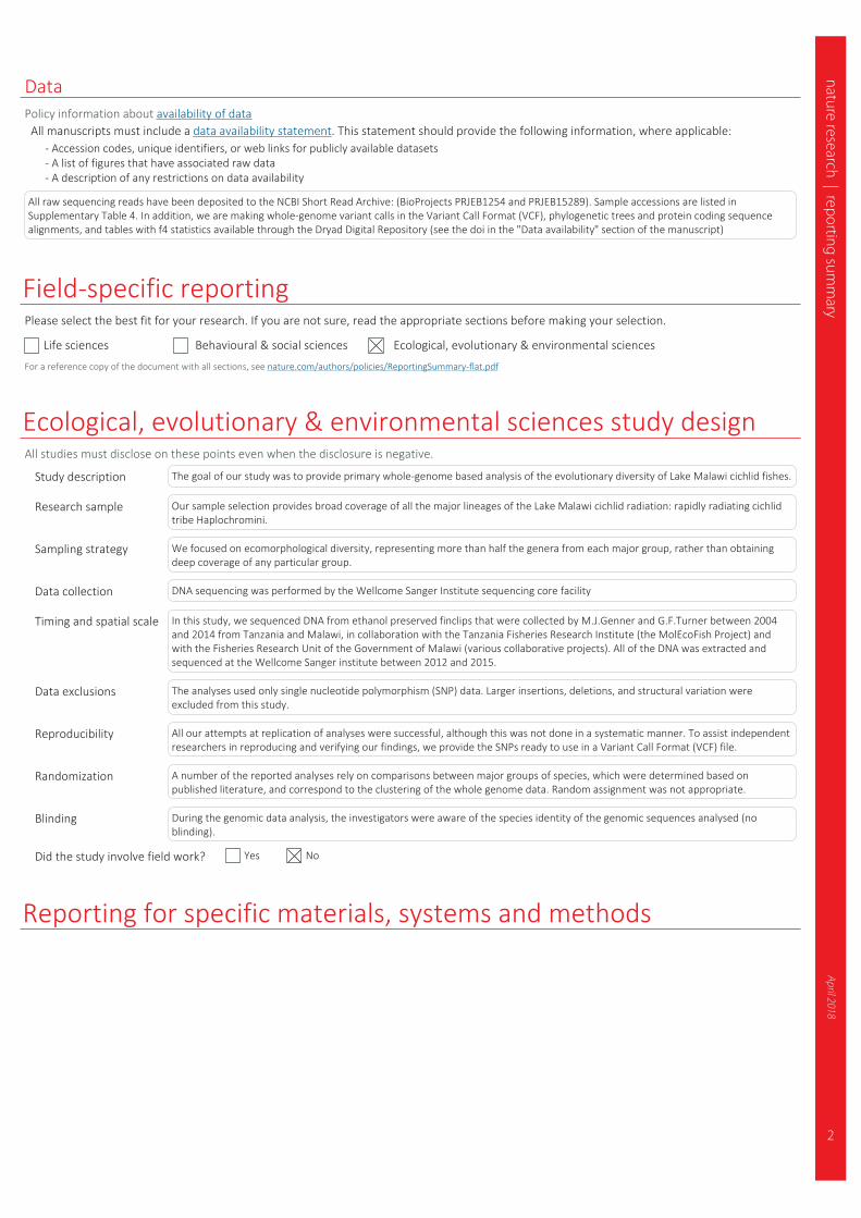
2

nature research | reporting summ

aryApril 2018

DataPolicy information about availability of data

All manuscripts must include a data availability statement. This statement should provide the following information, where applicable: - Accession codes, unique identifiers, or web links for publicly available datasets - A list of figures that have associated raw data - A description of any restrictions on data availability

All raw sequencing reads have been deposited to the NCBI Short Read Archive: (BioProjects PRJEB1254 and PRJEB15289). Sample accessions are listed in Supplementary Table 4. In addition, we are making whole-genome variant calls in the Variant Call Format (VCF), phylogenetic trees and protein coding sequence alignments, and tables with f4 statistics available through the Dryad Digital Repository (see the doi in the "Data availability" section of the manuscript)

Field-specific reportingPlease select the best fit for your research. If you are not sure, read the appropriate sections before making your selection.

Life sciences Behavioural & social sciences Ecological, evolutionary & environmental sciences

For a reference copy of the document with all sections, see nature.com/authors/policies/ReportingSummary-flat.pdf

Ecological, evolutionary & environmental sciences study designAll studies must disclose on these points even when the disclosure is negative.

Study description The goal of our study was to provide primary whole-genome based analysis of the evolutionary diversity of Lake Malawi cichlid fishes.

Research sample Our sample selection provides broad coverage of all the major lineages of the Lake Malawi cichlid radiation: rapidly radiating cichlid tribe Haplochromini.

Sampling strategy We focused on ecomorphological diversity, representing more than half the genera from each major group, rather than obtaining deep coverage of any particular group.

Data collection DNA sequencing was performed by the Wellcome Sanger Institute sequencing core facility

Timing and spatial scale In this study, we sequenced DNA from ethanol preserved finclips that were collected by M.J.Genner and G.F.Turner between 2004 and 2014 from Tanzania and Malawi, in collaboration with the Tanzania Fisheries Research Institute (the MolEcoFish Project) and with the Fisheries Research Unit of the Government of Malawi (various collaborative projects). All of the DNA was extracted and sequenced at the Wellcome Sanger institute between 2012 and 2015.

Data exclusions The analyses used only single nucleotide polymorphism (SNP) data. Larger insertions, deletions, and structural variation were excluded from this study.

Reproducibility All our attempts at replication of analyses were successful, although this was not done in a systematic manner. To assist independent researchers in reproducing and verifying our findings, we provide the SNPs ready to use in a Variant Call Format (VCF) file.

Randomization A number of the reported analyses rely on comparisons between major groups of species, which were determined based on published literature, and correspond to the clustering of the whole genome data. Random assignment was not appropriate.

Blinding During the genomic data analysis, the investigators were aware of the species identity of the genomic sequences analysed (no blinding).

Did the study involve field work? Yes No

Reporting for specific materials, systems and methods

3

nature research | reporting summ

aryApril 2018

Materials & experimental systemsn/a Involved in the study

Unique biological materials

Antibodies

Eukaryotic cell lines

Palaeontology

Animals and other organisms

Human research participants

Methodsn/a Involved in the study

ChIP-seq

Flow cytometry

MRI-based neuroimaging

Animals and other organismsPolicy information about studies involving animals; ARRIVE guidelines recommended for reporting animal research

Laboratory animals Trios were obtained by mating wild-caught fish obtained from Lake Malawi by commercial aquarium fish exporters (Stuart M. Grant Ltd) and exported to UK ornamental fish importers. Adults were quarantined at Bangor University's research aquarium, maintained at ca 25C in filtered aquaria with a mix of salts added to mimic Lake Malawi water conditions, and fed on standard aquarium fish flake food. Multiple females (5-10) were kept with a single adult male, until a female was seen to be carrying eggs (indicated by her bulging throat and loss of interest in food). Mouthbrooding females were removed to brooding tanks containing shelter for mother in the form of a PVC tube and shelter for the offspring in the form of rocks and artificial plants. When free-swimming fry were observed in the tank (usually after about 3 weeks), the mother was removed and, along with the father, euthanised by anaesthetic (MS-222) overdose. Offspring were reared for 3-6 months, before euthanasia.

Wild animals The study did not involve wild animals.

Field-collected samples Finclips were preserved in ethanol for DNA extraction.