No. 727 – 2007

Norsk Utenrikspolitisk Institutt

Norwegian Institute of International

Affairs

[727] Working Paper

Leo A. GrünfeldFrancesca Sanna-Randaccio

Who Buys Whom in International Oligopolies with FDI and Technology

Transfer?

Utgiver: Copyright:

ISSN:ISBN:

Besøksadresse:Addresse:

Internett:E-post:

Fax:Tel:

NUPI© Norsk Utenrikspolitisk Institutt 200782-7002-173-3978-82-7002-173-4Alle synspunkter står for forfatternes regning. De må ikke tolkes som uttrykk for oppfatninger som kan tillegges Norsk Utenrikspolitisk Institutt. Artiklene kan ikke reproduseres – helt eller delvis – ved trykking, fotokopiering eller på annen måte uten tillatelse fra forfatterne.

Any views expressed in this publication are those of the author. They should not be interpreted as reflecting the views of the Norwegian Institute of International Affairs. The text may not be printed in part or in full without the permission of the author.

C.J. Hambrosplass 2dPostboks 8159 Dep. 0033 Oslo www.nupi.nopub@nupi.no[+ 47] 22 36 21 82[+ 47] 22 99 40 00

[Abstract] Under what conditions will a technology leader from a small country acquire a laggard from a large country, and vice versa? We answer this question with a two-firm two-country Cournot model, where firms enter new markets via greenfield FDI or acqui-sition. The model takes into account both technological and market size asymmetries, and allows for M&A transaction costs, like corporate finance and legal fees. We show that to be the acquirer, a firm from a small country needs not only a strong technological lead but also the ability to exploit it on a global scale, which requires low international technolo-gy transfer costs. Moreover, we find that a multilateral greenfield investment liberalization may actually increase the incentives for foreign acquisitions. The effect of such liberaliza-tion on the nationality of the acquirer depends largely on the extent of the technology gap.

JEL classifications: L13, F23, O31, O38Keywords: Multinational firms, FDI, mergers and acquisitions (M&A), Technology transfer

Who buys whom in International Oligopolies with FDI and Technology

Leo A. GrünfeldMENON Business Economics / NUPITrosterudvn. 33b, N-0778, Oslo, NorwayE-mail: leo@menon.no Tel: 47-41105133

Francesca Sanna-RandaccioUniversity of Rome “La Sapienza”Via Buonarroti 1200185 Rome, ItalyE-mail: fsr@dis.uniroma1.itTel: 39-06-48299228Fax : 39-06-48299218

6 June 2007

Transfer?1

1 The two authors acknowledge support by the Norwegian Research Council (grant no.161422/I50), the Höegh Foundation and University of Rome ‘La Sapienza’. We also gratefully acknowledge the com-ments from participants at the ETSG 2005 conference in Dublin, the EIBA 2006 conference in Oslo, the EARIE 2006 conference in Amsterdam, the CNR conference in Milan and the RIEF conference in Rome.

5

WHO BUYS WHOM IN INTERNATIONAL OLIGOPOLIES WITH FDI AND TECHNOLOGY TRANSFER?

1. Introduction

The internationalisation of firms has assumed two new features. First, firms increasingly enter foreign

markets by acquiring a local producer rather than through greenfield FDI. The pattern is particularly

pronounced in industrialized host countries. Acquisitions accounted for 90% of inward FDI in the US1 in

1998 (UNCTAD (2000)). Most of such investments are directed towards the service sector, not

manufacturing, as in the past. In fact, while in the early 1970s services accounted for only one quarter of

the world FDI stock, this share had risen to about 60% in 2002 (UNCTAD (2004)). Out of 35.000 M&As

registered by Thomson Financial during the period 1995 to 2005, more than half were found in the

service sectors. Second, the interaction between the international strategy and the innovative activity of

firms has become increasingly tight and complex, due to the key role of multinational companies

(MNEs) in the process of generating and transferring technology and knowledge in the global market.

Models should therefore capture the technological implications of cross-border acquisitions.

The theoretical literature in economics has not devoted much focus to these important trends.

Most of the formal modelling of the internationalization of firms is still devoted to explain the drivers

and effects of greenfield FDI in the manufacturing sector (Horstmann and Markusen (1992); Petit and

Sanna-Randaccio (2000); Barba Navaretti and Venables (2004); Grünfeld (2006)). Such models cannot

help analyzing these recent trends for several reasons. To start with, as opposed to manufactured

products, most services are not tradable, thus the traditional way in which these models are framed (the

choice between export and FDI) cannot be applied to the internationalization of service. Second, while

greenfield FDI is considered, foreign entry via acquisition is not accounted for. As a consequence, what

is now the bulk of FDI activity remains unexplored.

Foreign acquisitions are often subject to intense public debate, especially if the takeover is

directed towards service sectors, where foreign ownership traditionally has been less pronounced (e.g

utilities and local transportation). During the last decades, a large number of technologically advanced

firms in smaller industrialized economies have been acquired by firms with larger home markets like the

US and UK. Many of these acquired firms were technology leaders and could, under the right conditions,

expand internationally on their own through greenfield investment or acquisitions abroad. However there

is also a fair amount of examples of advanced service sector firms from small markets expanding in

larger foreign markets through acquisitions. For instance, Belgian KBC bank acquired the relatively large

UK based financial firm Peel Hunt in 2001, the Austrian based advertising firm Lowe Lintas GGK

bought the British advertising firm Broadway Group one year earlier, while Danish Group 4 Falch

6

acquired French based Euroguard. According to Thomson Financial M&A database, more than 350

acquisitions in the service sectors involved a small country acquirer and a large country target during the

last 5 years.

In this paper, we identify the optimal foreign entry mode in a two country, two firm Cournot

model with asymmetric firm technology levels and asymmetric market (country) sizes. We are

particularly concerned with such asymmetries because the size of a market may affect the decision on

how to enter it. And moreover, the relative technological level of a firm also contributes to determine the

profitability of entering foreign markets. We specifically ask in which setting a technological leader from

a small country finds it optimal to buy a technologically inferior firm from a large country and vice-

versa. To answer this question, we develop a model that identifies the acquirer and the target firm. To our

knowledge, and somewhat surprisingly, there exists no such model which is applied to issues on

international M&As. Moreover, as opposed to the majority of earlier theoretical models on international

M&As, we explicitly allow for FDI running both ways between countries. This is a desirable property in

the case of industrialised countries, where multinationals often compete in each other’s home markets.

In the first stage of the model, firms simultaneously choose between no entry, greenfield FDI or

acquisition of the other firm. Notice that the model does not include exports as a strategic option. Thus, it

is best suited for studies of foreign entry into service sectors or manufacturing sectors where there are

high fixed and low variable export costs. In the second stage, firms set the profit maximizing level of

output. If a firm enters the foreign market through greenfield FDI, it has to pay a fixed investment cost

and its technology level in the foreign market is reduced due to technology transfer costs. If a firm enters

through acquisition, it must offer the other firm a sufficiently high acquisition price in order to obtain an

acceptance. If the bid is accepted through a Nash bargaining process, the acquirer becomes a monopolist

in both markets. The model is novel in this respect, as it combines a non-cooperative game relating to the

greenfield FDI decision, with a cooperative bargaining game where the potential acquisition and the

identity of the equilibrium acquirer is established.

If an acquisition takes place, the global monopolist may gain from three effects: a larger

monopoly rent, a best practice effect as better technology can be utilized in both countries, and finally

saving fixed plant costs associated with greenfield FDI. The model also captures that additional costs are

associated with the acquisition, e.g. due to legal and corporate finance fees.

The paper is organised as follows. In section 2, we briefly survey the relevant literature on this

subject and clarify what distinguishes our model from previous studies. Section 3 presents the model.

Section 4 analyzes the non-cooperative constrained game with a strategy space that excludes acquisition.

Section 5 analyses the acquisition decision in a cooperative game framework, by applying the Nash fixed

threat bargaining model. In Section 6, we analyse the equilibrium outcomes in the full model, partly

1 The figure refers to M&A however the same source indicates that acquisition dominates the scene, since less than 3% of cross-border acquisitions by number are mergers (UNCTAD (2000) p. 99).

7

based on analytical results and partly on numerical simulations. Finally, Section 7 presents the main

conclusions.

2. Earlier empirical and theoretical contributions

Numerous empirical studies, mainly undertaken in the 1990s, have analyzed the MNEs choice between

greenfield FDI and acquisition. The technological characteristics of the foreign investor emerge as an

important determinant of the entry mode. The R&D intensity of the investing firm appears to be

negatively related to the probability of an acquisition as compared to a greenfield FDI (Andersson and

Svensson (1994); Brouthres and Brouthres (2000); Harzing (2002)). This finding is explained as the

result of two factors. First, greenfield entry reduces the chance of technology dissemination in the foreign

country. Second, it may be more difficult to exploit abroad a superior technology implanting it in an

existing organisation than by creating a new one. The results are more mixed with respect to the impact

of the relative technological capability of the investor, versus the target firm. Kogut and Chang (1991)

analysed Japanese investments in the US at the industry level and found that Japanese acquisitions in the

US are insensitive to the difference in R&D expenditure in Japan and the US.2 On the other hand, Anand

and Delios (2002), considering 2175 entries by British, German and Japanese investors in the US, found

that the probability of entry via acquisition was positively affected by the difference in R&D

expenditure in the host and home country, indicating acquisitions motivated by technology sourcing.

As to the effect of home and host country characteristics, there is substantial agreement that the

cultural distance between home and host country decreases the probability of entry via acquisition as it

increases the cost of integrating the two company cultures (Kogut and Singh (1988); Barkema and

Vermeulen (1998); Harzing (2002)). However there is no concordance on other aspects. For instance, the

level of GDP per capita in the host economy is found to be positively and significantly related to the

probability of acquisition (Andersson and Svensson (1994)), but has a negative (although not significant)

effect in Barkema and Vermeulen (1998). Nor the size of the host country bears any clear impact.

Furthermore, mixed evidence is obtained on the influence of other factors such as foreign experience and

the degree of product diversification of the investor3.

The economic mechanisms associated with international acquisitions are clearly not yet fully

explained by the empirical literature, thus theoretical work may help to stimulate new directions for

empirical research.

Recently, a few theoretical papers have addressed the issue of Greenfield FDI via cross border

acquisition, but in these studies the identity of the acquirer is exogenously determined and the interplay

between asymmetries in the technology level of firms and the relative size of countries is not accounted

2 Similar results obtained by Anand and Kogut (1997) 3 As to the effect of foreign experience on the probability of foreing entry via acquisition or greenfield, Andersson and Svensson (1994) found a positive effetc; Barkema and Vermeulen (1998) and Brouthers and Brouthers (2000), found a negative effect and in Hennart and Park (1993) and Kogut and Singh (1988) this variable was not significant.

8

for. Moreover in most of these studies the acquisition has no effect on the profitability of the foreign

investor in the home country, and technology flows only from the foreign firm to the local ones, thus

excluding the possibility of technology sourcing FDI. Interesting insights may nevertheless be drawn

from this literature.4

These analyses predominantly assume only one way FDI. Mattoo, Olarreaga and Saggi (2004)

present a North-South model which highlights how the foreign firm’s choice between greenfield FDI or

acquisition and the local government’s ranking of the two modes are affected by the cost of technology

transfer within the MNE. Focusing on developed countries, Bjorvatn (2004) studies the effect of

economic integration on the profitability of international merger with two countries and three firms. Two

producers are located in a foreign country and are “active” as they decide how to expand abroad via

export, greenfield investment or acquisition, the third one in the national market is set to be the potential

acquisition target. The model shows that economic integration may stimulate international mergers by

lowering the reservation price of the target firm and by reducing the business stealing effect5, since the

outside firm (the “active” non merging firm) is more likely to choose export instead of greenfield FDI.

The impact that greenfield FDI barriers may have on the likelihood of an acquisition is analyzed also by

Norbäck and (2002). They consider the case in which a state-owned firm is privatized and sold in an

auction in which a local privately owned firm and a foreign MNE compete as buyers. The foreign firm

may enter the market via export, greenfield FDI or acquiring the privatized firm. The paper suggests that

high greenfield costs and high trade costs do not necessarily induce foreign acquisitions in privatization,

since the domestic firm can more easily prevent the foreign firm from becoming a strong local

competitor. Hence the willingness to pay of the domestic firm for the state assets is high.6 The

importance of entry threats by greenfield FDI and/or export is also highlighted be Eicher and Kang

(2005). Their three stage entry model based on Bertrand’s conjectures shows that very large markets are

likely to attract acquisitions due to large monopoly benefits, when entry threats by greenfield FDI

and/or export can be used.

Only a few studies consider two-way FDI, and the studies are framed in a symmetric context,

where the identity of the acquirer is undetermined. Horn and Persson (2001) analyze how the incentive to

form either domestic or international mergers is influenced by trade costs. They consider the choice

whether to export abroad or to acquire a foreign firm in a symmetric model with four firms. Greenfield

4 Recently, models based on new trade theory and firm heterogeneity have advanced further to explain the choice between export, Greenfield FDI and acquisition in foreign markets. See Nocke and Yeaple (2005) for more on this. 5 This effect is due to firms not participating to the merger expanding their production and therefore stealing business from merging partners. 6 See also Görg (2000). He analyses whether a technologically advantaged firm, which has decided to undertake an FDI in a foreign market, will enter via greenfield investment or acquisition, and in the latter case whether to acquire the local low technology or the high technology firm. The analysis shows that under most conditions the take-over of the existing indigenous high technology firm is the preferred market entry mode.

9

FDI is not allowed for, thus making the model less relevant for most service sectors. They find that high

trade barriers induce domestic rather than international mergers contrary to the tariff jumping argument.7

Several important questions thus remain unanswered: how to determine endogenously the

identity of the acquirer; what are the roles of technological and country size asymmetries and what is the

effect of greenfield FDI liberalisation and ICT improvements on the equilibrium mode of entry.

3. The model The model consists of two countries (I and II) and two firms, (1 and 2), that produce a homogeneous

service or good in country I and II respectively. Countries may vary in size and firms may differ as to

cost reducing exogenous technology as in Fosfuri and Motta (1999).8 Firms determine the mode of

foreign entry, choosing among three possible strategies: no expansion abroad (N), greenfield FDI (G) or

full acquisition9 of the foreign firm (Ai), i=1,2 where i represents the acquirer.

We assume that the total technology pool is divided between the two firms in proportion σ for

firm 1 and ( σ−1 ) for firm 2 with [ ]1,0∈σ . Unit variable costs in the home market for firm 1 and 2,

respectively under the strategies N and G, are simply:

σ−= 0,1 cc I (1)

)1(0,2 σ−−= cc II (2)

where the parameter 10 ≥c guarantees non-negative costs. We assume that there is no involuntary

dissemination of knowledge (no external spillovers) when the two firms are under separate ownership.10

The unit variable costs of production abroad under G are given by:

τσ−= 0,1 cc II (3)

)1(0,2 στ −−= cc I (4)

showing that cross border internal know how transfer from parent to subsidiary is costly. The costs of

internal knowledge transfer are inversely related to the parameter [ ]1,0∈τ . It follows that if 1<τ , the

subsidiary is always less efficient than its parent. If a firm chooses G, it also faces a fixed set up cost F in

the foreign market.

If firm 1 makes the acquisition, unit variable production cost in country I and II respectively are:

7 Ferret (2003) analyses cross border acquisitions in an international duopoly with a third potential player deciding on entry. The model shows that acquisitions are more likely in medium sized markets where entry does not occur (thus implying that with the growth of the world economy acquisitions will tend to slow). 8 Fosfuri and Motta (1999) present a Cournot duopoly model where firms may choose to service the foreign market either through exports or greenfield FDI. We bring this model one step further, by allowing firms to enter the foreign market through an acquisition. 9 Here we do not allow firms to involve in a merger where the parties own a percentage share of the firm. Such a possibility will complicate the model since we both will have to specify merger price and a sharing rate of profits between parties. Mattoo et al. (2004) also show that the equilibrium M&A always is a 100% acquisition. 10 This is a strong assumption that simplifies the model vastly. Yet since we operate with technology transfer when acquisition is the strategy, allowing for no transfer under G, can simply be viewed as a relative benchmarking of the technology transfer under different entry modes.

10

{ }[ ])1(,max0,1 στσ −−= cc I (5)

{ }[ ])1(,max0,1 στσ −−= cc II (6)

while if firm 2 makes the acquisition we have:

{ }[ ]τσσ ),1(max0,2 −−= cc II (7)

{ }[ ])1(,max0,2 στσ −−= cc I (8)

Equations (5)-(8) rest on the assumption of a best practise effect (the term in the square brackets). That is

to say, we assume that the new company adopts in each market what is the most efficient technology

between that available in-house and that available in the target company. However, if foreign technology

is implemented in a firm, there will be a loss due to technology transfer costs. An acquisition also

requires additional acquisition transaction costs which will be discussed in section 5.1.

We assume linear (inverse) demand functions:

IIII Qasqqp −=+ )( ,2,1 (9)

IIIIIIII Qsaqqp −−=+ )1()( ,2,1 (10)

where JJJ qqQ ,2,1 += for J=I,II. The parameter a represents the joint size of the two markets while the

parameter )1,0(∈s indicates the share of a accounted for by country I, and (1-s) the share by country II.

The profits of the two firms differ depending on the strategy combinations ),( 21 λλ with

{ }AiGNii ,,=Λ∈λ . Six equilibrium strategies may arise: )(NN where each firm produce and sell

only in the home market; )(GN ( )(NG ) where firm 1 (2) conducts a greenfield FDI while the rival

operates only in the domestic market; )(GG where we have a MNE duopoly; )0,1(A where firm 1

acquires firm 2, and finally )2,0( A where firm 2 acquires firm 1. The profit functions are reported in

Appendix I.

We identify the optimal foreign entry mode by solving a two stage game. In the first stage, firms

decide upon the mode of entry. This is done in two steps. We first find the non-cooperative solution to a

constrained game with strategy space { }GNi ,~=Λ ignoring acquisition as a strategy. We call this the

status quo game. The solution to this game defines the threat point (alternative profits if no agreement)

in the cooperative acquisition game, where we identify whether there will be an acquisition and who

buys whom. The cooperative game is solved using the Nash fixed-threat bargaining equilibrium concept.

In the second stage, firms set their profit maximizing level of output. As usual, the game is solved by

backwards induction.

4. The status quo game We first describe the non-cooperative status quo game with the constrained strategy space { }GNi ,~

=Λ .

Firm specific equilibrium profit functions for the four possible strategy combinations are reported in

11

Appendix II. By comparing equilibrium profits under alternative strategy combinations, we can identify

the condition for a dominant strategy:

[ ]F

cas>

−−+−−9

)1(2)1( 20 στσ

(11)

[ ]F

csa>

−−+−9

)1(2 20 σστ

(12)

If (11) is satisfied, G is the dominant strategy for firm 1. Otherwise, N will be the dominant

strategy.11 Similarly, if (12) holds, G will be the dominant strategy for firm 2.12 The probability that (11)

(alternatively(12)) holds is decreasing (increasing) in s (the relative size of market I):

[ ]0

9)1(2)1(2)11( 0 <

−−+−−−=

∂∂ στσcas

as

LHS (13)

[ ]0

9)1(22)12( 0 >

−−+−=

∂∂ σστcsa

as

LHS (14)

This finding reminds us that a large host market (ceteris paribus) is an important attractor for inward

greenfield FDI since it implies higher variable profits, to compensate for the additional fixed plant costs

(F). Similarly, a larger total market (a) gives stronger incentives for greenfield FDI.

The probability that (11) (alternatively(12)) holds is increasing (decreasing) inσ (the relative

technology level of firm 1):

[ ]0

9)1(2)1(2

)12()11( 0 >−−+−−

+=∂

∂ στστ

σcasLHS (15)

[ ]0

9)1(22

)12()12( 0 <−−+−

+−=∂

∂ σσττ

σcsaLHS (16)

So the technologically leading firm is more likely to expand abroad than the weaker competitor. Its

variable cost advantage implies that by producing abroad it will enjoy –ceteris paribus- higher variable

profits than its competitor. The advantage of the leading firm is greater the lower the cost of cross border

technology transfer (the higherτ ) since low internal technology transfer costs imply that the leading firm

will benefit more in the foreign market from its technological leadership.

11 If (11) holds, we have that: NGGG

11 ˆˆ ππ > and NNGN11 ˆˆ ππ >

12 If (12) holds, we have that: NNNG

22 ˆˆ ππ > and GNGG22 ˆˆ ππ >

12

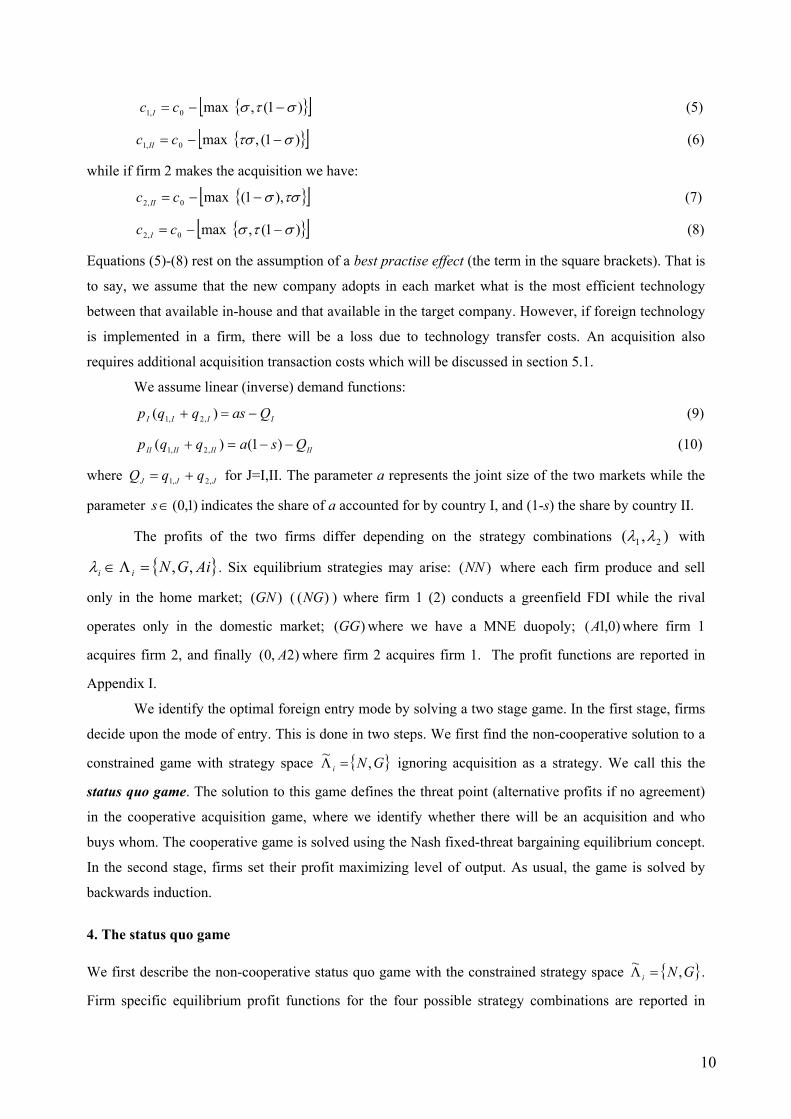
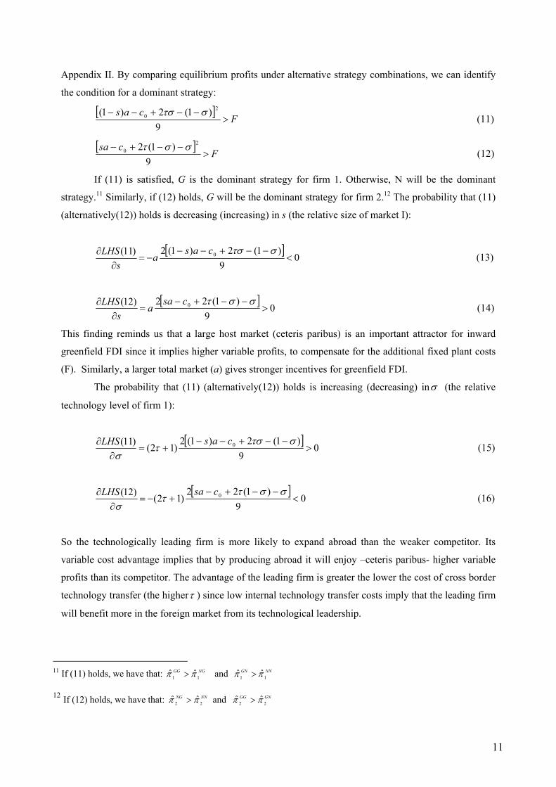
The Nash equilibrium strategy configuration in the status quo game ( *~Λ ) clearly depends on the

value of the parameters. Fig 1a and 1b illustrates how *~Λ depends on the value of s andσ , where the

fixed investment cost (F) is set to 1.5 and 0.5 in Fig 1a and 1b respectively.13

Figure 1a: Regions defining equilibrium outcomes in the ( σ,s ) plane with F=1.5

Figure 1b: Regions defining equilibrium outcomes in the ( σ,s ) plane with F=0.5

13 In these figures, a=3,τ=0.5 and .10 =c

NG

GG

0

0.2

0.4

0.6

0.8

1

s

0.2 0.4 0.6 0.8 1sigma

NN

NG

0

0.2

0.4

0.6

0.8

1

s

0.2 0.4 0.6 0.8 1sigma

NG

GG

GN

GN

13

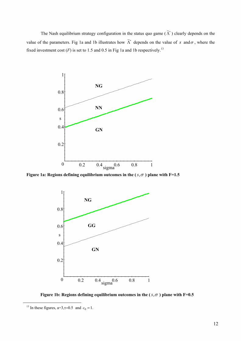
The thick line in figures 1a and 1b represents condition (11)14 with strict equality, whereas the

thin line represents condition (12)15. In the case where firm 1 has a technology advantage and its

foreign market is relatively large (south-east in the diagrams), it will chose G, while firm 2 will

chose N. By symmetry, the opposite strategies are chosen in the north-west corner of the

diagrams. When F is reduced, these two indifference lines shift upwards and downwards

respectively, and when they shift positions, the equilibrium changes from NN in Figure 1a to

GG in Figure 1b. Since the two indifference lines are always parallel, no parameter combination

allows both GG and NN to be equilibrium within the feasible ),( σs space. If we reduce

knowledge transfer costs (increase τ ), the indifference lines become steeper, as illustrated in

Figure 2. Hence, an increase in τ contributes to a larger area where .~* GG=Λ

Figure 2: Changes in the regions defining equilibrium outcomes in the ( σ,s ) plane with an

increase in τ

14 Eq.(11) can be rearranged as: στaa

Fcas )12(310 +

+−−−

<

15 Eq.(12) can be rearranged as: σττaa

Fcs )12(320 +

++−

>

0

0.2

0.4

0.6

0.8

1

s

0.2 0.4 0.6 0.8 1sigma

GN

NG

GG

14

5. Bargaining for an acquisition 5.1 The equilibrium bid

We first identify the equilibrium offer or bid ( iB ) when firm i wants to acquire firm j . The problem can

be solve as a cooperative game16, using the Nash fixed – threat bargaining model (see Friedman 1990;

Petit, 1990). The players bargain on how to divide the profits associated with the acquisition. The status

quo equilibrium *~Λ provides the payoffs obtained by the players if they fail to make an agreement, called

the disagreement outcomes or status quo profits ),( dj

di ππ .

The profit of the acquirer (firm i) is given by:

iiAi

iAii BTV −−=Π (17)

where AiiV represents the gross profits of the global monopolist (see Appendix I). Notice that

AAjj

Aii VVV == since both firms face exactly the same markets and technology as a global monopolist.

Due to the best practise effect, unit cost in each market does not depend on which firm makes the

acquisition. Consequently, from here on we drop the firm specific notation for AV . To calculate the net

profit of the acquirer, we must subtract iT which represents transaction costs associated with the deal, as

well as the acquisition price iB paid to j. Transaction costs associated with an acquisition ( iT ) arise due to

legal fees, consulting fees and corporate finance costs, as well as costs related to the integration of the

two work forces and to the managerial resources to be devoted to the acquisition. We model the

transaction costs as a linear function of the size of the deal, which in turn is a function of the target firm

capitalisation. This is equivalent to the target firm status quo profits:

djiT γπ= where 1> 0>γ (18)

The profits of the target firm are equal to the acquisition price:

iAij B=Π (19)

The equilibrium bid iB is given by the Nash bargaining solution of the cooperative game described in

Appendix III. With constant marginal utility of profits, the bargaining solution provides the standard

result that excess profits from the acquisition (i.e. the overall gain from cooperation) is evenly divided

between the two players. Thus, profits for the target firm becomes

{ } [ ]di

dj

Adj

di

dj

Adj

Aiji VVB ππγππγππ −−+=+−−+=Π= )1(

21)()(

21 (20)

where the term in curly brackets represents the overall gain from cooperation. The acquisition price paid

for the target firm reflects what firm j profits could have become if the acquisition did not take place.

As to the acquirer, firm i will earn the following profits:

16 This way of dealing with the problem is in line with the empirical finding that the overwhelming number of M&A both domestic and international are friendly rather than hostile takeovers.

15

{ } [ ]di

dj

Adj

di

dj

Adi

Aii VV ππγππγππ ++−=+−−+=Π )1(

21)()(

21 (21)

which represents the status quo profit plus the bargaining share of firm i. The profits from acquisition for

both firms are increasing in the global monopolist profits, increasing in own status quo profits, but

decreasing in the rival’s status quo profits.

5.2 Condition for a cross border acquisition to take place

An acquisition equilibrium requires that both firms gain from it as compared to the status quo

equilibrium profit, that is di

Aii π>Π and d

jAij π>Π . We find, using (20) and (21), that both these

conditions are satisfied iff: di

dj

AV ππγ ++> )1( (22)

If there are excess profits from the acquisition made by firm i, the acquisition will take place since both

firms will benefit from it. 17 This leads us to the following proposition:

Proposition 1:

An acquisition will take place if the gross profit from the acquisition ( AV ) is larger than the sum of the

two firms’ status quo profits plus the transaction costs.

5.3 Condition for being the acquirer

We know that firm i would like to be the acquirer if its profit is higher than the profit it receives from

being the target, that is if Aji

Aii Π>Π , which implies from (20) and (21) that:

[ ] [ ]dj

di

Adi

dj

A VV ππγππγ −−+>++− )1(21)1(

21 (23)

which can be reduced to: dj

di ππ > (24)

The same condition applies to Ajj

Aij Π>Π , so we have that Ai is the optimal entry mode ( Ai=Λ* )

iff dj

di ππ > . We can thus state:

Proposition 2:

It is always the firm with the highest status quo profit that becomes the acquirer, regardless of the size of

01 >> γ .

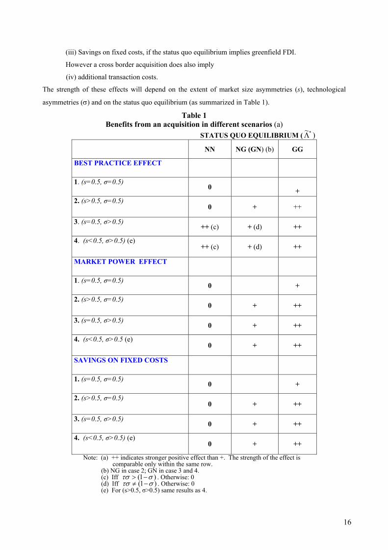
To sum up, an acquisition brings the following benefits and costs compared to greenfield entry:

(i) Market power effect

(ii) Best practice effect (providing lower unit variable cost.)

17 This is the traditional criterion for merger incentive in the IO literature, which however overlooks transaction costs. See e.g. Horn and Persson (2001).

16

(iii) Savings on fixed costs, if the status quo equilibrium implies greenfield FDI.

However a cross border acquisition does also imply

(iv) additional transaction costs.

The strength of these effects will depend on the extent of market size asymmetries (s), technological

asymmetries (σ) and on the status quo equilibrium (as summarized in Table 1).

Table 1 Benefits from an acquisition in different scenarios (a)

STATUS QUO EQUILIBRIUM ( *~Λ )

NN NG (GN) (b) GG

BEST PRACTICE EFFECT

1. (s=0.5, σ=0.5) 0

+ 2. (s>0.5, σ=0.5)

0 + ++

3. (s=0.5, σ>0.5) ++ (c) + (d) ++

4. (s<0.5, σ>0.5) (e)

++ (c) + (d) ++

MARKET POWER EFFECT

1. (s=0.5, σ=0.5) 0 +

2. (s>0.5, σ=0.5)

0 + ++

3. (s=0.5, σ>0.5) 0 + ++

4. (s<0.5, σ>0.5 (e)

0 + ++

SAVINGS ON FIXED COSTS

1. (s=0.5, σ=0.5) 0 +

2. (s>0.5, σ=0.5)

0 + ++

3. (s=0.5, σ>0.5) 0 + ++

4. (s<0.5, σ>0.5) (e)

0 + ++

Note: (a) ++ indicates stronger positive effect than +. The strength of the effect is comparable only within the same row. (b) NG in case 2; GN in case 3 and 4. (c) Iff )1( στσ −> . Otherwise: 0 (d) Iff )1( στσ −≠ . Otherwise: 0 (e) For (s>0.5, σ>0.5) same results as 4.

17

6. Equilibrium solution to the full game We initially present analytical results and then revert to simulations. In Figures 4-7, simulation results are

presented for the different combinations of firm characteristics in the ( σ,s ) space. In the upper half of

each matrix, country I is the largest, while it is the smallest in the lower half. We focus our attention to

the range [ )1,5.0∈σ where firm 1 is a technological leader, since this region represents all relevant

combinations of technologies and market sizes. In the figures, the left hand matrix illustrates simulation

results for the status quo game, while the right hand matrix provides the solution to the full game. In the

following discussion, we start out with the simplest case where firms and countries are symmetric, and

then add asymmetries as we go along.

6.1 Full symmetry (s=0.5, σ=0.5)

In the case of both market size and technology symmetry, the left hand side of conditions (11) and (12)

become identical, thus )(~* NN=Λ and )(~* GG=Λ are the only feasible solutions. It is not possible to

identify a potential acquirer since dj

di ππ = . An acquisition generates a monopoly in both countries and

since the best practice technology will always be 5.0=σ we have that: NNi

AV π2= (25)

If )(~* NN=Λ , the profit of the acquirer is given by:

[ ] NNi

NNi

NNi

NNj

AAii V ππγππγ <−=++−=Π )5.01()1((

21 (26)

Thus under full symmetry, profits from the acquisition will always be lower than profits from the status-

quo NN equilibrium. In such scenario foreign entry by acquisition is not feasible as none of the potential

benefits from an acquisition (best practise, increased market power, saving on fixed cost) will be at work

to compensate for transaction costs (see Table 1). However, this does not have to be the case if

)(~* GG=Λ ,due to technology transfer costs, stronger competition, and F (plant fixed cost). If

)(~* GG=Λ , the condition for a cross border acquisition to take place (Eq. (22)) becomes:

GGi

GGi

NNi

πππ

γ)(2 −

< (27)

implying that an acquisition is feasible in equilibrium under full symmetry since GGi

NNi ππ > for all

parameter values. Note that )(~* GG=Λ may materialize even though both firms get higher profits from

NN, as we may face a prisoner’s dilemma situation. It follows that:

18

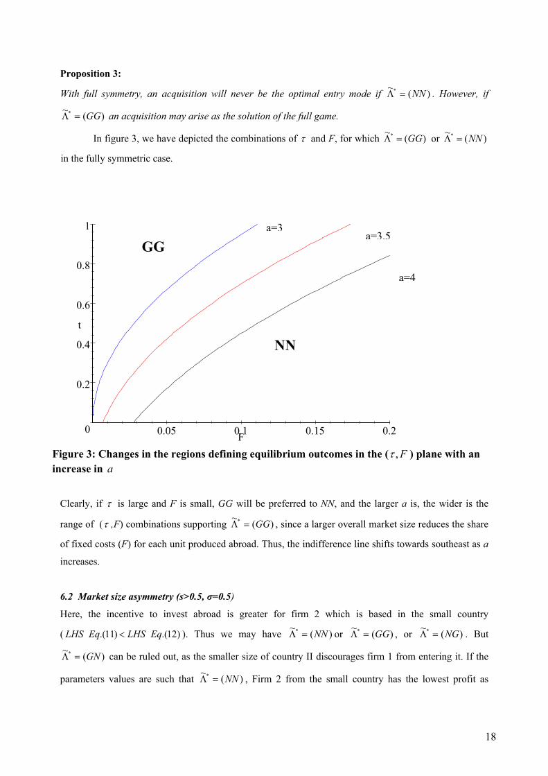
Proposition 3:

With full symmetry, an acquisition will never be the optimal entry mode if )(~* NN=Λ . However, if

)(~* GG=Λ an acquisition may arise as the solution of the full game.

In figure 3, we have depicted the combinations of τ and F, for which )(~* GG=Λ or )(~* NN=Λ

in the fully symmetric case.

Figure 3: Changes in the regions defining equilibrium outcomes in the ( F,τ ) plane with an increase in a

Clearly, if τ is large and F is small, GG will be preferred to NN, and the larger a is, the wider is the

range of (τ ,F) combinations supporting )(~* GG=Λ , since a larger overall market size reduces the share

of fixed costs (F) for each unit produced abroad. Thus, the indifference line shifts towards southeast as a

increases.

6.2 Market size asymmetry (s>0.5, σ=0.5)

Here, the incentive to invest abroad is greater for firm 2 which is based in the small country

( )12.()11.( EqLHSEqLHS < ). Thus we may have )(~* NN=Λ or )(~* GG=Λ , or )(~* NG=Λ . But

)(~* GN=Λ can be ruled out, as the smaller size of country II discourages firm 1 from entering it. If the

parameters values are such that )(~* NN=Λ , Firm 2 from the small country has the lowest profit as

0

0.2

0.4

0.6

0.8

1

t

0.05 0.1 0.15 0.2F

GG

NN

a=3

a=4

a=3.5

19

5.0>σ . This will also be the case if )(~* GG=Λ when 1<τ , since firm 2 will have a cost disadvantage

in the large market due to the cost of internal technology transfer.18 Simulation results show that if

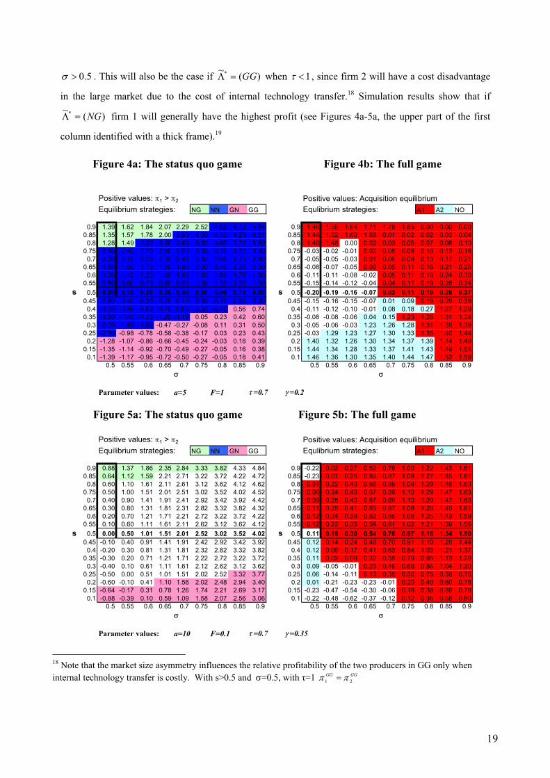
)(~* NG=Λ firm 1 will generally have the highest profit (see Figures 4a-5a, the upper part of the first

column identified with a thick frame).19

Figure 4a: The status quo game Figure 4b: The full game

Positive values: π1 > π2 Positive values: Acquisition equilibriumEquilibrium strategies: NG NN GN GG Equlibrium strategies: A1 A2 NO

0.9 1.39 1.62 1.84 2.07 2.29 2.52 4.62 4.73 4.84 0.9 1.46 1.55 1.64 1.71 1.78 1.85 0.00 0.00 0.000.85 1.35 1.57 1.78 2.00 3.90 4.00 4.10 4.20 4.31 0.85 1.44 1.52 1.60 1.68 0.01 0.02 0.02 0.03 0.04

0.8 1.28 1.49 3.20 3.30 3.40 3.50 3.60 3.70 3.80 0.8 1.40 1.48 0.00 0.02 0.03 0.05 0.07 0.08 0.100.75 2.50 2.60 2.70 2.80 2.90 3.00 3.10 3.20 3.30 0.75 -0.03 -0.02 -0.01 0.02 0.05 0.08 0.10 0.13 0.16

0.7 2.00 2.10 2.20 2.30 2.40 2.50 2.60 2.70 2.80 0.7 -0.05 -0.05 -0.03 0.01 0.05 0.09 0.13 0.17 0.210.65 1.50 1.60 1.70 1.80 1.90 2.00 2.10 2.20 2.30 0.65 -0.08 -0.07 -0.05 0.00 0.05 0.11 0.16 0.21 0.26

0.6 1.00 1.10 1.20 1.30 1.40 1.50 1.60 1.70 1.80 0.6 -0.11 -0.11 -0.08 -0.02 0.05 0.11 0.18 0.24 0.300.55 0.50 0.60 0.70 0.80 0.90 1.00 1.10 1.20 1.30 0.55 -0.15 -0.14 -0.12 -0.04 0.04 0.11 0.19 0.26 0.34

s 0.5 -0.00 0.10 0.20 0.30 0.40 0.50 0.60 0.70 0.80 s 0.5 -0.20 -0.19 -0.16 -0.07 0.02 0.11 0.19 0.28 0.370.45 -0.50 -0.40 -0.30 -0.20 -0.10 -0.00 0.10 0.20 0.30 0.45 -0.15 -0.16 -0.15 -0.07 0.01 0.09 0.19 0.29 0.39

0.4 -1.00 -0.90 -0.80 -0.70 -0.60 -0.50 -0.40 0.56 0.74 0.4 -0.11 -0.12 -0.10 -0.01 0.08 0.18 0.27 1.27 1.290.35 -1.50 -1.40 -1.30 -1.20 -1.10 0.05 0.23 0.42 0.60 0.35 -0.08 -0.08 -0.06 0.04 0.15 1.23 1.28 1.31 1.34

0.3 -2.00 -1.90 -1.80 -0.47 -0.27 -0.08 0.11 0.31 0.50 0.3 -0.05 -0.06 -0.03 1.23 1.26 1.28 1.31 1.35 1.390.25 -2.50 -0.98 -0.78 -0.58 -0.38 -0.17 0.03 0.23 0.43 0.25 -0.03 1.29 1.23 1.27 1.30 1.33 1.35 1.40 1.44

0.2 -1.28 -1.07 -0.86 -0.66 -0.45 -0.24 -0.03 0.18 0.39 0.2 1.40 1.32 1.26 1.30 1.34 1.37 1.39 1.44 1.490.15 -1.35 -1.14 -0.92 -0.70 -0.49 -0.27 -0.05 0.16 0.38 0.15 1.44 1.34 1.28 1.33 1.37 1.41 1.43 1.49 1.54

0.1 -1.39 -1.17 -0.95 -0.72 -0.50 -0.27 -0.05 0.18 0.41 0.1 1.46 1.36 1.30 1.35 1.40 1.44 1.47 1.53 1.590.5 0.55 0.6 0.65 0.7 0.75 0.8 0.85 0.9 0.5 0.55 0.6 0.65 0.7 0.75 0.8 0.85 0.9

σ σ

Parameter values: a=5 F=1 τ =0.7 γ =0.2 Figure 5a: The status quo game Figure 5b: The full game

Positive values: π1 > π2 Positive values: Acquisition equilibriumEquilibrium strategies: NG NN GN GG Equlibrium strategies: A1 A2 NO

0.9 0.88 1.37 1.86 2.35 2.84 3.33 3.82 4.33 4.84 0.9 -0.22 0.02 0.27 0.52 0.76 1.00 1.22 1.43 1.610.85 0.64 1.12 1.59 2.21 2.71 3.22 3.72 4.22 4.72 0.85 -0.23 0.01 0.25 0.65 0.87 1.08 1.27 1.45 1.61

0.8 0.60 1.10 1.61 2.11 2.61 3.12 3.62 4.12 4.62 0.8 0.01 0.22 0.43 0.66 0.89 1.09 1.29 1.46 1.630.75 0.50 1.00 1.51 2.01 2.51 3.02 3.52 4.02 4.52 0.75 0.06 0.24 0.43 0.67 0.89 1.10 1.29 1.47 1.63

0.7 0.40 0.90 1.41 1.91 2.41 2.92 3.42 3.92 4.42 0.7 0.09 0.25 0.43 0.67 0.89 1.10 1.29 1.47 1.630.65 0.30 0.80 1.31 1.81 2.31 2.82 3.32 3.82 4.32 0.65 0.11 0.25 0.41 0.65 0.87 1.08 1.28 1.45 1.61

0.6 0.20 0.70 1.21 1.71 2.21 2.72 3.22 3.72 4.22 0.6 0.12 0.24 0.39 0.62 0.85 1.06 1.25 1.43 1.590.55 0.10 0.60 1.11 1.61 2.11 2.62 3.12 3.62 4.12 0.55 0.12 0.22 0.35 0.59 0.81 1.02 1.21 1.39 1.55

s 0.5 0.00 0.50 1.01 1.51 2.01 2.52 3.02 3.52 4.02 s 0.5 0.11 0.19 0.30 0.54 0.76 0.97 1.16 1.34 1.500.45 -0.10 0.40 0.91 1.41 1.91 2.42 2.92 3.42 3.92 0.45 0.12 0.14 0.24 0.48 0.70 0.91 1.10 1.28 1.44

0.4 -0.20 0.30 0.81 1.31 1.81 2.32 2.82 3.32 3.82 0.4 0.12 0.09 0.17 0.41 0.63 0.84 1.03 1.21 1.370.35 -0.30 0.20 0.71 1.21 1.71 2.22 2.72 3.22 3.72 0.35 0.11 0.02 0.09 0.32 0.55 0.76 0.95 1.13 1.29

0.3 -0.40 0.10 0.61 1.11 1.61 2.12 2.62 3.12 3.62 0.3 0.09 -0.05 -0.01 0.23 0.46 0.66 0.86 1.04 1.200.25 -0.50 0.00 0.51 1.01 1.51 2.02 2.52 3.32 3.77 0.25 0.06 -0.14 -0.11 0.13 0.35 0.56 0.75 0.59 0.76

0.2 -0.60 -0.10 0.41 1.10 1.56 2.02 2.48 2.94 3.40 0.2 0.01 -0.21 -0.23 -0.23 -0.01 0.20 0.40 0.60 0.780.15 -0.64 -0.17 0.31 0.78 1.26 1.74 2.21 2.69 3.17 0.15 -0.23 -0.47 -0.54 -0.30 -0.06 0.16 0.38 0.59 0.79

0.1 -0.88 -0.39 0.10 0.59 1.09 1.58 2.07 2.56 3.06 0.1 -0.22 -0.48 -0.62 -0.37 -0.12 0.12 0.36 0.58 0.800.5 0.55 0.6 0.65 0.7 0.75 0.8 0.85 0.9 0.5 0.55 0.6 0.65 0.7 0.75 0.8 0.85 0.9

σ σ

Parameter values: a=10 F=0.1 τ =0.7 γ =0.35

18 Note that the market size asymmetry influences the relative profitability of the two producers in GG only when internal technology transfer is costly. With s>0.5 and σ=0.5, with τ=1 GGGG

21 ππ =

20

Turning to the solution of the full game, as in the completely symmetric case, if )(~* NN=Λ no

acquisition may take place because there will be no best practice, market power, or fixed cost saving

effects20. If )(~* GG=Λ , an acquisition may take place, but only )1(* A=Λ is feasible since we know

from above that GGGG21 ππ > . The results are confirmed by simulations in table 4-5. It follows that:

Proposition 4:

Market asymmetry alone (i.e. when 5.0=σ ) is not sufficient to stimulate a cross border acquisition

when the threat is represented by two national monopolies. If the status quo equilibrium is GG, an

acquisition may take place and the acquirer will be the firm from the large country.

6.3 Technological asymmetry (s=0.5, σ>0.5)

It is now necessary to take into consideration the best practice effect under acquisition. Firm 1, which is

the technology leader, has a larger incentive to invest abroad due to lower variable costs. The feasible

status quo equilibria are thus NN, GG and GN, while NG can be ruled out since

)12.()11.( EqLHSEqLHS > . Here, the acquisition gross profit can be defined as the sum of the national

monopoly profits plus the gains through adoption of the best practice (k).

kV NNNNA ++= 21 ˆˆ ππ where (28)

k =[ ] [ ]{ }

−>>−−+−−−−

−<

)1(0)1()()1()1(241

)1( 0

220 στσστσστσ

στσ

iffcas

iff (29)

Thus due to the best practice effect, technology asymmetry alone (i.e. with 5.0=s ) provides incentives

for an acquisition, also when the alternative to an acquisition is represented by two national monopolies.

Notice that in the previous section, we found that market size asymmetry alone is not sufficient to trigger

an acquisition when )(~* NN=Λ , but technology asymmetry is. An acquisition equilibrium will arise if

the best practice effect fully compensates for the acquisition transaction costs, which requires from Eq.

(22) that NNk 2π̂γ> . Notice that the probability of an acquisition is increasing in the technological

asymmetry, since 0>∂∂σk (consult the central row with a thick frame in Figures 4b for illustrations).21

We can thus state:

19 In a few cases (that is if the difference between the size of the two markets is rather small and τ is high), we may have ngng

12 ˆˆ ππ > . The likelihood that 012 >− NGNG ππ is increasing in τ and decreasing in s (see Appendix IV). 20 Due to σ=0.5 NNNNAV 21 ππ += and Eqs (28) and (29) are valid also in this scenario. 21 Figure 5 shows that an acquisition may take place also when )(~ * GGS = or )(~* GNS = .

21

Proposition 5: In the case of technological asymmetry and market size symmetry, an acquisition can

take place also when )(~* NN=Λ .

As to the identity of the acquirer, we can state the following22 (proof in Appendix V):

Proposition 6:

In the case of technological asymmetry and market size symmetry, the acquirer will always be the

technology leader.

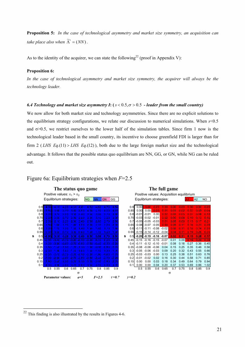
6.4 Technology and market size asymmetry I: ( 5.0,5.0 >< σs - leader from the small country)

We now allow for both market size and technology asymmetries. Since there are no explicit solutions to

the equilibrium strategy configurations, we relate our discussion to numerical simulations. When s<0.5

and σ>0.5, we restrict ourselves to the lower half of the simulation tables. Since firm 1 now is the

technological leader based in the small country, its incentive to choose greenfield FDI is larger than for

firm 2 ( )12.()11.( EqLHSEqLHS > ), both due to the large foreign market size and the technological

advantage. It follows that the possible status quo equilibrium are NN, GG, or GN, while NG can be ruled

out.

Figure 6a: Equilibrium strategies when F=2.5

The status quo game The full game Positive values: π1 > π2 Positive values: Acquisition equilibriumEquilibrium strategies: NG NN GN GG Equlibrium strategies: A1 A2 NO

0.9 4.00 4.10 4.20 4.31 4.41 4.52 4.62 4.73 4.84 0.9 0.00 0.00 0.00 0.00 0.00 0.00 0.00 0.00 0.000.85 3.50 3.60 3.70 3.80 3.90 4.00 4.10 4.20 4.31 0.85 0.00 0.00 0.00 0.01 0.01 0.02 0.02 0.03 0.04

0.8 3.00 3.10 3.20 3.30 3.40 3.50 3.60 3.70 3.80 0.8 -0.01 -0.01 0.00 0.02 0.03 0.05 0.07 0.08 0.100.75 2.50 2.60 2.70 2.80 2.90 3.00 3.10 3.20 3.30 0.75 -0.03 -0.02 -0.01 0.02 0.05 0.08 0.10 0.13 0.16

0.7 2.00 2.10 2.20 2.30 2.40 2.50 2.60 2.70 2.80 0.7 -0.05 -0.05 -0.03 0.01 0.05 0.09 0.13 0.17 0.210.65 1.50 1.60 1.70 1.80 1.90 2.00 2.10 2.20 2.30 0.65 -0.08 -0.07 -0.05 0.00 0.05 0.11 0.16 0.21 0.26

0.6 1.00 1.10 1.20 1.30 1.40 1.50 1.60 1.70 1.80 0.6 -0.11 -0.11 -0.08 -0.02 0.05 0.11 0.18 0.24 0.300.55 0.50 0.60 0.70 0.80 0.90 1.00 1.10 1.20 1.30 0.55 -0.15 -0.14 -0.12 -0.04 0.04 0.11 0.19 0.26 0.34

s 0.5 -0.00 0.10 0.20 0.30 0.40 0.50 0.60 0.70 0.80 s 0.5 -0.20 -0.19 -0.16 -0.07 0.02 0.11 0.19 0.28 0.370.45 -0.50 -0.40 -0.30 -0.20 -0.10 -0.00 0.10 0.20 0.30 0.45 -0.15 -0.16 -0.15 -0.07 0.01 0.09 0.19 0.29 0.39

0.4 -1.00 -0.90 -0.80 -0.70 -0.60 -0.50 -0.40 -0.30 -0.20 0.4 -0.11 -0.12 -0.10 -0.01 0.08 0.18 0.27 0.36 0.450.35 -1.50 -1.40 -1.30 -1.20 -1.10 -1.00 -0.90 -0.80 -0.70 0.35 -0.08 -0.08 -0.06 0.04 0.15 0.25 0.35 0.46 0.56

0.3 -2.00 -1.90 -1.80 -1.70 -1.60 -1.50 -1.40 -1.30 -1.20 0.3 -0.05 -0.06 -0.03 0.09 0.20 0.32 0.43 0.55 0.660.25 -2.50 -2.40 -2.30 -2.20 -2.10 -2.00 -1.90 -1.80 -1.70 0.25 -0.03 -0.03 0.00 0.13 0.25 0.38 0.51 0.63 0.76

0.2 -3.00 -2.90 -2.80 -2.70 -2.60 -2.50 -2.40 -2.30 -2.20 0.2 -0.01 -0.02 0.02 0.16 0.30 0.44 0.58 0.71 0.850.15 -3.50 -3.40 -3.30 -3.20 -3.10 -3.00 -2.90 -2.80 -2.70 0.15 0.00 0.00 0.03 0.18 0.34 0.49 0.64 0.79 0.94

0.1 -4.00 -3.90 -3.80 -3.70 -3.60 -3.50 -3.40 -3.30 -3.20 0.1 0.00 0.00 0.04 0.20 0.37 0.53 0.69 0.86 1.020.5 0.55 0.6 0.65 0.7 0.75 0.8 0.85 0.9 0.5 0.55 0.6 0.65 0.7 0.75 0.8 0.85 0.9

σ σParameter values: a=5 F=2.5 τ =0.7 γ =0.2

22 This finding is also illustrated by the results in Figures 4-6.

22

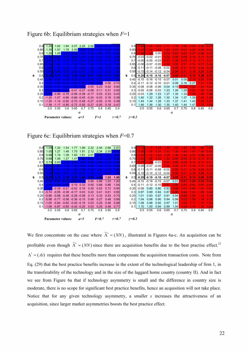
Figure 6b: Equilibrium strategies when F=1

0.9 1.39 1.62 1.84 2.07 2.29 2.52 4.62 4.73 4.84 0.9 1.46 1.55 1.64 1.71 1.78 1.85 0.00 0.00 0.000.85 1.35 1.57 1.78 2.00 3.90 4.00 4.10 4.20 4.31 0.85 1.44 1.52 1.60 1.68 0.01 0.02 0.02 0.03 0.04

0.8 1.28 1.49 3.20 3.30 3.40 3.50 3.60 3.70 3.80 0.8 1.40 1.48 0.00 0.02 0.03 0.05 0.07 0.08 0.100.75 2.50 2.60 2.70 2.80 2.90 3.00 3.10 3.20 3.30 0.75 -0.03 -0.02 -0.01 0.02 0.05 0.08 0.10 0.13 0.16

0.7 2.00 2.10 2.20 2.30 2.40 2.50 2.60 2.70 2.80 0.7 -0.05 -0.05 -0.03 0.01 0.05 0.09 0.13 0.17 0.210.65 1.50 1.60 1.70 1.80 1.90 2.00 2.10 2.20 2.30 0.65 -0.08 -0.07 -0.05 0.00 0.05 0.11 0.16 0.21 0.26

0.6 1.00 1.10 1.20 1.30 1.40 1.50 1.60 1.70 1.80 0.6 -0.11 -0.11 -0.08 -0.02 0.05 0.11 0.18 0.24 0.300.55 0.50 0.60 0.70 0.80 0.90 1.00 1.10 1.20 1.30 0.55 -0.15 -0.14 -0.12 -0.04 0.04 0.11 0.19 0.26 0.34

s 0.5 -0.00 0.10 0.20 0.30 0.40 0.50 0.60 0.70 0.80 s 0.5 -0.20 -0.19 -0.16 -0.07 0.02 0.11 0.19 0.28 0.370.45 -0.50 -0.40 -0.30 -0.20 -0.10 -0.00 0.10 0.20 0.30 0.45 -0.15 -0.16 -0.15 -0.07 0.01 0.09 0.19 0.29 0.39

0.4 -1.00 -0.90 -0.80 -0.70 -0.60 -0.50 -0.40 0.56 0.74 0.4 -0.11 -0.12 -0.10 -0.01 0.08 0.18 0.27 1.27 1.290.35 -1.50 -1.40 -1.30 -1.20 -1.10 0.05 0.23 0.42 0.60 0.35 -0.08 -0.08 -0.06 0.04 0.15 1.23 1.28 1.31 1.34

0.3 -2.00 -1.90 -1.80 -0.47 -0.27 -0.08 0.11 0.31 0.50 0.3 -0.05 -0.06 -0.03 1.23 1.26 1.28 1.31 1.35 1.390.25 -2.50 -0.98 -0.78 -0.58 -0.38 -0.17 0.03 0.23 0.43 0.25 -0.03 1.29 1.23 1.27 1.30 1.33 1.35 1.40 1.44

0.2 -1.28 -1.07 -0.86 -0.66 -0.45 -0.24 -0.03 0.18 0.39 0.2 1.40 1.32 1.26 1.30 1.34 1.37 1.39 1.44 1.490.15 -1.35 -1.14 -0.92 -0.70 -0.49 -0.27 -0.05 0.16 0.38 0.15 1.44 1.34 1.28 1.33 1.37 1.41 1.43 1.49 1.54

0.1 -1.39 -1.17 -0.95 -0.72 -0.50 -0.27 -0.05 0.18 0.41 0.1 1.46 1.36 1.30 1.35 1.40 1.44 1.47 1.53 1.590.5 0.55 0.6 0.65 0.7 0.75 0.8 0.85 0.9 0.5 0.55 0.6 0.65 0.7 0.75 0.8 0.85 0.9

σ σParameter values: a=5 F=1 τ =0.7 γ =0.2

Figure 6c: Equilibrium strategies when F=0.7

0.9 1.09 1.32 1.54 1.77 1.99 2.22 2.45 2.68 2.91 0.9 1.10 1.19 1.28 1.35 1.42 1.49 1.55 1.60 1.640.85 1.05 1.27 1.48 1.70 1.91 2.12 2.34 2.55 4.31 0.85 1.08 1.16 1.24 1.32 1.39 1.45 1.51 1.56 0.04

0.8 0.98 1.19 1.39 1.60 1.81 2.01 3.60 3.70 3.80 0.8 1.04 1.12 1.20 1.28 1.36 1.43 0.07 0.08 0.100.75 0.88 1.08 1.27 1.47 2.90 3.00 3.10 3.20 3.30 0.75 1.01 1.08 1.16 1.24 0.05 0.08 0.10 0.13 0.16

0.7 0.74 0.93 2.20 2.30 2.40 2.50 2.60 2.70 2.80 0.7 0.97 1.03 -0.03 0.01 0.05 0.09 0.13 0.17 0.210.65 1.50 1.60 1.70 1.80 1.90 2.00 2.10 2.20 2.30 0.65 -0.08 -0.07 -0.05 0.00 0.05 0.11 0.16 0.21 0.26

0.6 1.00 1.10 1.20 1.30 1.40 1.50 1.60 1.70 1.80 0.6 -0.11 -0.11 -0.08 -0.02 0.05 0.11 0.18 0.24 0.300.55 0.50 0.60 0.70 0.80 0.90 1.00 1.10 1.20 1.30 0.55 -0.15 -0.14 -0.12 -0.04 0.04 0.11 0.19 0.26 0.34

s 0.5 -0.00 0.10 0.20 0.30 0.40 0.50 0.60 1.24 1.40 s 0.5 -0.20 -0.19 -0.16 -0.07 0.02 0.11 0.19 0.89 0.900.45 -0.50 -0.40 -0.30 -0.20 -0.10 0.69 0.86 1.03 1.20 0.45 -0.15 -0.16 -0.15 -0.07 0.01 0.87 0.90 0.93 0.94

0.4 -1.00 -0.90 -0.80 0.15 0.33 0.50 0.68 0.86 1.04 0.4 -0.11 -0.12 -0.10 0.81 0.86 0.90 0.94 0.97 0.990.35 -1.50 -0.39 -0.21 -0.02 0.16 0.35 0.53 0.72 0.90 0.35 -0.08 0.85 0.80 0.83 0.88 0.93 0.98 1.01 1.04

0.3 -0.74 -0.55 -0.36 -0.17 0.03 0.22 0.41 0.61 0.80 0.3 0.97 0.89 0.84 0.87 0.90 0.96 1.01 1.05 1.090.25 -0.88 -0.68 -0.48 -0.28 -0.08 0.13 0.33 0.53 0.73 0.25 1.01 0.93 0.87 0.91 0.94 0.99 1.05 1.10 1.14

0.2 -0.98 -0.77 -0.56 -0.36 -0.15 0.06 0.27 0.48 0.69 0.2 1.04 0.96 0.90 0.94 0.98 1.02 1.09 1.14 1.190.15 -1.05 -0.84 -0.62 -0.40 -0.19 0.03 0.25 0.46 0.68 0.15 1.08 0.98 0.92 0.97 1.01 1.05 1.12 1.19 1.24

0.1 -1.09 -0.87 -0.65 -0.42 -0.20 0.03 0.25 0.48 0.71 0.1 1.10 1.00 0.94 0.99 1.04 1.09 1.16 1.23 1.290.5 0.55 0.6 0.65 0.7 0.75 0.8 0.85 0.9 0.5 0.55 0.6 0.65 0.7 0.75 0.8 0.85 0.9

σ σParameter values: a=5 F=0.7 τ =0.7 γ =0.2

We first concentrate on the case where )(~* NN=Λ , illustrated in Figures 6a-c. An acquisition can be

profitable even though )(~* NN=Λ since there are acquisition benefits due to the best practise effect.23

)(* Ai=Λ requires that these benefits more than compensate the acquisition transaction costs. Note from

Eq. (29) that the best practice benefits increase in the extent of the technological leadership of firm 1, in

the transferability of the technology and in the size of the laggard home country (country II). And in fact

we see from Figure 6a that if technology asymmetry is small and the difference in country size is

moderate, there is no scope for significant best practice benefits, hence an acquisition will not take place.

Notice that for any given technology asymmetry, a smaller s increases the attractiveness of an

acquisition, since larger market asymmetries boosts the best practice effect.

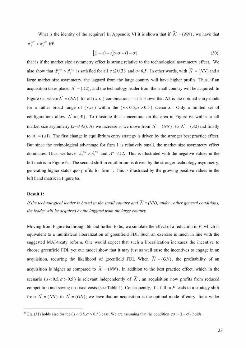
23

What is the identity of the acquirer? In Appendix VI it is shown that if )(~* NN=Λ , we have that

NNNN12 ˆˆ ππ > iff:

[ ] )1()1( σσ −−>−− ss (30)

that is if the market size asymmetry effect is strong relative to the technological asymmetry effect. We

also show that NNNN12 ˆˆ ππ > is satisfied for all 33.0≤s and σ>0.5. In other words, with )(~* NN=Λ and a

large market size asymmetry, the laggard from the large country will have higher profits. Thus, if an

acquisition takes place, )2(* A=Λ , and the technology leader from the small country will be acquired. In

Figure 6a, where )(~* NN=Λ for all ( σ,s ) combinations – it is shown that A2 is the optimal entry mode

for a rather broad range of ( σ,s ) within the ( 5.0,5.0 >< σs ) scenario. Only a limited set of

configurations allow )1(* A=Λ . To illustrate this, concentrate on the area in Figure 6a with a small

market size asymmetry (s=0.45). As we increase σ, we move from )(* NN=Λ , to )2(* A=Λ and finally

to )1(* A=Λ . The first change in equilibrium entry strategy is driven by the stronger best practice effect.

But since the technological advantage for firm 1 is relatively small, the market size asymmetry effect

dominates. Thus, we have NNNN12 ˆˆ ππ > and Λ*=(A2). This is illustrated with the negative values in the

left matrix in Figure 6a. The second shift in equilibrium is driven by the stronger technology asymmetry,

generating higher status quo profits for firm 1. This is illustrated by the growing positive values in the

left hand matrix in Figure 6a.

Result 1:

If the technological leader is based in the small country and *~Λ =(NN), under rather general conditions,

the leader will be acquired by the laggard from the large country.

Moving from Figure 6a through 6b and further to 6c, we simulate the effect of a reduction in F, which is

equivalent to a multilateral liberalization of greenfield FDI. Such an exercise is much in line with the

suggested MAI-treaty reform. One would expect that such a liberalization increases the incentive to

choose greenfield FDI, yet our model show that it may just as well raise the incentives to engage in an

acquisition, reducing the likelihood of greenfield FDI. When )(~* GN=Λ , the profitability of an

acquisition is higher as compared to )(~* NN=Λ . In addition to the best practice effect, which in the

scenario ( 5.0,5.0 >< σs ) is relevant independently of *~Λ , an acquisition now profits from reduced

competition and saving on fixed costs (see Table 1). Consequently, if a fall in F leads to a strategy shift

from )(~* NN=Λ to )(~* GN=Λ , we have that an acquisition is the optimal mode of entry for a wider

23 Eq. (31) holds also for the ( 5.0,5.0 >< σs ) case. We are assuming that the condition )1( στσ −> holds.

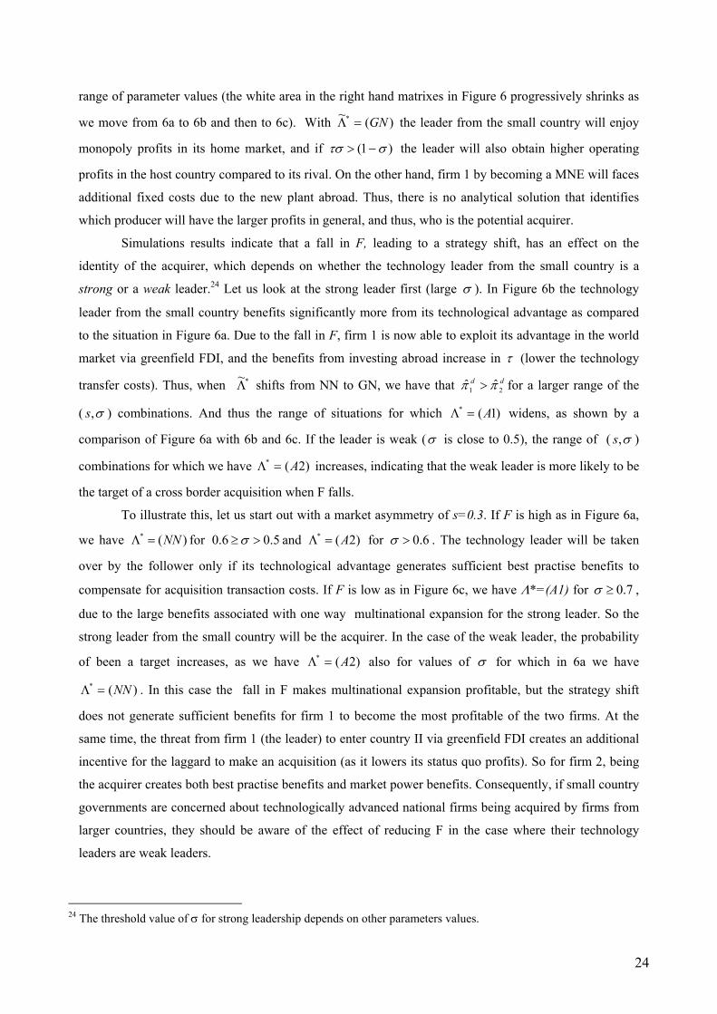
24

range of parameter values (the white area in the right hand matrixes in Figure 6 progressively shrinks as

we move from 6a to 6b and then to 6c). With )(~* GN=Λ the leader from the small country will enjoy

monopoly profits in its home market, and if )1( στσ −> the leader will also obtain higher operating

profits in the host country compared to its rival. On the other hand, firm 1 by becoming a MNE will faces

additional fixed costs due to the new plant abroad. Thus, there is no analytical solution that identifies

which producer will have the larger profits in general, and thus, who is the potential acquirer.

Simulations results indicate that a fall in F, leading to a strategy shift, has an effect on the

identity of the acquirer, which depends on whether the technology leader from the small country is a

strong or a weak leader.24 Let us look at the strong leader first (large σ ). In Figure 6b the technology

leader from the small country benefits significantly more from its technological advantage as compared

to the situation in Figure 6a. Due to the fall in F, firm 1 is now able to exploit its advantage in the world

market via greenfield FDI, and the benefits from investing abroad increase in τ (lower the technology

transfer costs). Thus, when *~Λ shifts from NN to GN, we have that dd

21 ˆˆ ππ > for a larger range of the

( σ,s ) combinations. And thus the range of situations for which )1(* A=Λ widens, as shown by a

comparison of Figure 6a with 6b and 6c. If the leader is weak (σ is close to 0.5), the range of ( σ,s )

combinations for which we have )2(* A=Λ increases, indicating that the weak leader is more likely to be

the target of a cross border acquisition when F falls.

To illustrate this, let us start out with a market asymmetry of s=0.3. If F is high as in Figure 6a,

we have )(* NN=Λ for 5.06.0 >≥ σ and )2(* A=Λ for 6.0>σ . The technology leader will be taken

over by the follower only if its technological advantage generates sufficient best practise benefits to

compensate for acquisition transaction costs. If F is low as in Figure 6c, we have Λ*=(A1) for 7.0≥σ ,

due to the large benefits associated with one way multinational expansion for the strong leader. So the

strong leader from the small country will be the acquirer. In the case of the weak leader, the probability

of been a target increases, as we have )2(* A=Λ also for values of σ for which in 6a we have

)(* NN=Λ . In this case the fall in F makes multinational expansion profitable, but the strategy shift

does not generate sufficient benefits for firm 1 to become the most profitable of the two firms. At the

same time, the threat from firm 1 (the leader) to enter country II via greenfield FDI creates an additional

incentive for the laggard to make an acquisition (as it lowers its status quo profits). So for firm 2, being

the acquirer creates both best practise benefits and market power benefits. Consequently, if small country

governments are concerned about technologically advanced national firms being acquired by firms from

larger countries, they should be aware of the effect of reducing F in the case where their technology

leaders are weak leaders.

24 The threshold value of σ for strong leadership depends on other parameters values.

25

Result 2:

Multilateral greenfield FDI liberalization (i.e. a reduction in F) increases the likelihood of an

acquisition, as compared to the case of segmented markets (i.e. )(~* NN=Λ )25.

Result 3:

If the technological leader is based in the small country, the effect of multilateral greenfield FDI

liberalization on the identity of the acquirer depends on the extent of the technological gap. If firm 1 is a

weak technology leader (σ close to 0,5), its probability of being acquired by the laggard increases. If it

is a strong technology leader, its probability of acquiring the laggard from the large market increases.

If the threat is cross-greenfield FDI ( )(~* GG=Λ ), the gains from an acquisition are further enlarged as

saving on fixed costs is doubled and the gains from reduced competition relates to both markets (see

Table 1). Hence, only if acquisition costs are large, the firms will decide not to merge (consult the

simulations in Figure 5 where Λ*=(Ai) for most parameter combinations even though γ is as large as

0.35). Furthermore, if )1( στσ −> , the leader from the small country will always be the acquirer

( )1(* A=Λ ), since it will have higher operating profits due to a better technology in both markets, while

facing the same fixed costs.

In Figure 7 we simulate a reduction in technology transfer costs (higherτ ) which may be due to

technological development in ICT or to greater attention devoted by firms to know-how management.

The effects are similar to those driven by a fall in F. Moving from Figure 7a to 7b, we see that as τ

increases, the white area (i.e. the non acquisition area) shrinks. It becomes relatively more profitable for

the technology leader to go multinational, and the smaller the transfer costs are, the higher will its profit

be relative to the opponent. Furthermore, the effect on the identity of the acquirer is also similar to the

effect from a fall in F. If you start out from s=0.3 in Figure 7a and cut transfer costs (see 7b), you will

move from )(* NN=Λ to Λ*=(A2) if the firm 1 is a weak technology leader, while you move from

)2(* A=Λ to )1(* A=Λ if firm 1 is a strong technology leader.

25 This result holds also for the other scenarios considered.

26

Figure 7a: Equilibrium strategies when 7.0=τ

The status quo game The full game

Positive values: π1 > π2 Positive values: Acquisition equilibriumEquilibrium strategies: NG NN GN GG Equlibrium strategies: A1 A2 NO

0,9 1,39 1,62 1,84 2,07 2,29 2,52 4,62 4,73 4,84 0,9 1,46 1,55 1,64 1,71 1,78 1,85 0,00 0,00 0,000,85 1,35 1,57 1,78 2,00 3,90 4,00 4,10 4,20 4,31 0,85 1,44 1,52 1,60 1,68 0,01 0,02 0,02 0,03 0,040,8 1,28 1,49 3,20 3,30 3,40 3,50 3,60 3,70 3,80 0,8 1,40 1,48 0,00 0,02 0,03 0,05 0,07 0,08 0,10

0,75 2,50 2,60 2,70 2,80 2,90 3,00 3,10 3,20 3,30 0,75 -0,03 -0,02 -0,01 0,02 0,05 0,08 0,10 0,13 0,160,7 2,00 2,10 2,20 2,30 2,40 2,50 2,60 2,70 2,80 0,7 -0,05 -0,05 -0,03 0,01 0,05 0,09 0,13 0,17 0,21

0,65 1,50 1,60 1,70 1,80 1,90 2,00 2,10 2,20 2,30 0,65 -0,08 -0,07 -0,05 0,00 0,05 0,11 0,16 0,21 0,260,6 1,00 1,10 1,20 1,30 1,40 1,50 1,60 1,70 1,80 0,6 -0,11 -0,11 -0,08 -0,02 0,05 0,11 0,18 0,24 0,30

0,55 0,50 0,60 0,70 0,80 0,90 1,00 1,10 1,20 1,30 0,55 -0,15 -0,14 -0,12 -0,04 0,04 0,11 0,19 0,26 0,34 s 0,5 -0,00 0,10 0,20 0,30 0,40 0,50 0,60 0,70 0,80 s 0,5 -0,20 -0,19 -0,16 -0,07 0,02 0,11 0,19 0,28 0,37

0,45 -0,50 -0,40 -0,30 -0,20 -0,10 -0,00 0,10 0,20 0,30 0,45 -0,15 -0,16 -0,15 -0,07 0,01 0,09 0,19 0,29 0,390,4 -1,00 -0,90 -0,80 -0,70 -0,60 -0,50 -0,40 0,56 0,74 0,4 -0,11 -0,12 -0,10 -0,01 0,08 0,18 0,27 1,27 1,29

0,35 -1,50 -1,40 -1,30 -1,20 -1,10 0,05 0,23 0,42 0,60 0,35 -0,08 -0,08 -0,06 0,04 0,15 1,23 1,28 1,31 1,340,3 -2,00 -1,90 -1,80 -0,47 -0,27 -0,08 0,11 0,31 0,50 0,3 -0,05 -0,06 -0,03 1,23 1,26 1,28 1,31 1,35 1,39

0,25 -2,50 -0,98 -0,78 -0,58 -0,38 -0,17 0,03 0,23 0,43 0,25 -0,03 1,29 1,23 1,27 1,30 1,33 1,35 1,40 1,440,2 -1,28 -1,07 -0,86 -0,66 -0,45 -0,24 -0,03 0,18 0,39 0,2 1,40 1,32 1,26 1,30 1,34 1,37 1,39 1,44 1,49

0,15 -1,35 -1,14 -0,92 -0,70 -0,49 -0,27 -0,05 0,16 0,38 0,15 1,44 1,34 1,28 1,33 1,37 1,41 1,43 1,49 1,540,1 -1,39 -1,17 -0,95 -0,72 -0,50 -0,27 -0,05 0,18 0,41 0,1 1,46 1,36 1,30 1,35 1,40 1,44 1,47 1,53 1,59

0,5 0,55 0,6 0,65 0,7 0,75 0,8 0,85 0,9 0,5 0,55 0,6 0,65 0,7 0,75 0,8 0,85 0,9σ σ

Parameter values: a=5 F=1 τ =0.7 γ =0.2 Figure 7b: Equilibrium strategies when 1=τ

Positive values: π1 > π2 Positive values: Acquisition equilibriumEquilibrium strategies: NG NN GN GG Equlibrium strategies: A1 A2 NO

0,9 1,00 1,27 1,53 1,80 2,07 2,33 2,60 4,73 4,84 0,9 1,29 1,41 1,53 1,63 1,73 1,82 1,90 0,03 0,040,85 0,98 1,24 1,49 1,75 2,00 4,00 4,10 4,20 4,31 0,85 1,28 1,40 1,52 1,63 1,73 0,06 0,08 0,09 0,110,8 0,94 1,18 1,43 1,67 3,40 3,50 3,60 3,70 3,80 0,8 1,26 1,39 1,51 1,63 0,10 0,12 0,15 0,17 0,20

0,75 0,86 1,09 2,70 2,80 2,90 3,00 3,10 3,20 3,30 0,75 1,23 1,37 0,05 0,09 0,13 0,18 0,21 0,25 0,290,7 2,00 2,10 2,20 2,30 2,40 2,50 2,60 2,70 2,80 0,7 -0,05 0,00 0,06 0,11 0,17 0,22 0,28 0,33 0,38

0,65 1,50 1,60 1,70 1,80 1,90 2,00 2,10 2,20 2,30 0,65 -0,08 -0,01 0,06 0,13 0,19 0,26 0,33 0,40 0,460,6 1,00 1,10 1,20 1,30 1,40 1,50 1,60 1,70 1,80 0,6 -0,11 -0,03 0,05 0,13 0,22 0,30 0,38 0,46 0,54

0,55 0,50 0,60 0,70 0,80 0,90 1,00 1,10 1,20 1,30 0,55 -0,15 -0,06 0,04 0,13 0,23 0,33 0,42 0,51 0,61 s 0,5 -0,00 0,10 0,20 0,30 0,40 0,50 0,60 1,31 1,51 s 0,5 -0,20 -0,09 0,02 0,13 0,24 0,35 0,46 1,23 1,22

0,45 -0,50 -0,40 -0,30 -0,20 -0,10 -0,00 0,95 1,15 1,36 0,45 -0,15 -0,05 0,05 0,16 0,26 0,36 1,28 1,29 1,290,4 -1,00 -0,90 -0,80 -0,70 0,39 0,60 0,81 1,02 1,24 0,4 -0,11 0,00 0,12 0,24 1,27 1,31 1,33 1,35 1,36

0,35 -1,50 -1,40 -0,18 0,04 0,26 0,48 0,70 0,92 1,15 0,35 -0,08 0,05 1,23 1,26 1,31 1,36 1,39 1,41 1,430,3 -2,00 -0,52 -0,30 -0,07 0,16 0,39 0,62 0,86 1,09 0,3 -0,05 1,25 1,28 1,31 1,35 1,40 1,44 1,48 1,50

0,25 -0,86 -0,62 -0,39 -0,15 0,09 0,33 0,58 0,82 1,06 0,25 1,23 1,28 1,32 1,35 1,39 1,45 1,50 1,54 1,570,2 -0,94 -0,69 -0,44 -0,19 0,06 0,31 0,56 0,81 1,07 0,2 1,26 1,31 1,36 1,40 1,43 1,50 1,56 1,61 1,64

0,15 -0,98 -0,73 -0,47 -0,21 0,05 0,31 0,58 0,84 1,11 0,15 1,28 1,34 1,39 1,43 1,48 1,55 1,62 1,67 1,720,1 -1,00 -0,73 -0,46 -0,19 0,08 0,35 0,62 0,90 1,17 0,1 1,29 1,36 1,42 1,46 1,52 1,60 1,67 1,74 1,79

0,5 0,55 0,6 0,65 0,7 0,75 0,8 0,85 0,9 0,5 0,55 0,6 0,65 0,7 0,75 0,8 0,85 0,9σ σ

Parameter values: a=5 F=1 τ =1 γ =0.2

27

6.5 Technology and market size asymmetry II: ( 5.0,5.0 >> σs - leader from the large country)

Firm 1 is the technological leader and is based in the large country. Market size and technological

effects run in the opposite direction. All the four status quo outcomes are possible (NN, GG, GN, GG).

If )(~* NN=Λ , firm 1 will have a larger profits; that is also the case in the GG outcome (see Figures 4 - 7

for illustrations). In the case of one way FDI, if the potential MNE is firm 1 (the GN case) here too firm

1 will have a larger status quo profit26. However, if the incentive from a large host market size prevail

(the NG case) due to the contrasting effect from technology and market size difference, we cannot have a

clear reply on which firm will have the largest status quo size and thus may become the acquirer.

Result 4:

In the case of a technology leader from a large country, under rather general conditions, this firm will be

the acquirer in case of a cross border take-over.

7. Conclusions In the theoretical industrial organisation literature, the study of why firms decide to enter a foreign

market through greenfield investment or M&As is in an infant stage. So far, no study has succeeded in

identifying what kind of firms chooses to make a cross border acquisition and what kind of firms chooses

instead to be acquired by foreign firms. In this paper we apply a simple bargaining model to determine

the identity of the acquirer, in a setting where firms differ with respect to technological level and

countries vary with respect to market size. We are thus able to analyse whether technology leaders from

small countries may find it optimal to acquire technology laggards from large countries, or vice versa.

Our model contains important features that seem to play a pivotal role in the choice between

conducting an acquisition or establishing a new subsidiary abroad through greenfield investment. We

consider the gains from implementing a best practice technology, and take into account knowledge

transfer costs and transaction costs associated with a merger due to legal fees, consulting fees and costs

of integrating the two company cultures. Empirical studies show that such acquisition costs can be

surprisingly high, leading to low profits from cross border acquisitions.

Our model shows that the acquiring firm is always the one that would have gained the highest

profits if an acquisition was not possible. In fact we find that the equilibrium acquisition price reflects the

target firm potential for growth. We also find that changes in the market size and technology

asymmetries affect the choice between cross border acquisition and other entry modes, both directly and

indirectly via strategy shifts, that is by inducing a change in what would be the equilibrium in the no

acquisition situation.

26 We have NNNN

21 ππ > which implies NNGN21 ππ > if the status quo is GN.

28

When only one type of asymmetry is considered, we find that if national markets are highly

protected and thus the alternative to an acquisition is represented by two national monopolies, market size

asymmetry alone does not generate an incentive for a cross border acquisition. However, technological

asymmetry alone may create such incentives. Furthermore, if we have technological asymmetry but market

size symmetry, when an acquisition takes place the technological leader is always the acquirer.

When both types of asymmetries play a role, we find that if the technology leader comes from a large

country, it will – except for some extreme configurations - be the acquirer if there is any cross border take

over at all. In the case of a technology leader based in the small country, the results are more complex. With

prohibitively high barriers to greenfield FDI (thus with. national monopolies in the non acquisition case),

under rather general conditions, if there is an acquisition that is made by the laggard based in the large

country. Market size asymmetry tends to prevail on technological asymmetry in such scenario, and a large

home market emerges as a key factor for determining who will be the acquirer in an international deal. Only

if market size asymmetry is rather small, an acquisition made by the technology leader may emerge as the

optimal entry mode within the segmented markets setting.

We also show that greenfield FDI liberalisation increases the likelihood of observing an acquisition

as the equilibrium outcome. In other words, if the globalization process leads to e.g. lower fixed investment

costs under greenfield, it does not necessarily mean that we will see more greenfield investment, but rather

more acquisitions. This prediction seems to fit the developments mentioned in Section 1. As to the identity of

the acquirer, we find that the effect of multilateral greenfield FDI liberalization depends on the extent of the

technology gap. If the small country producer enjoys a strong technological lead and is able to exploit it

internationally, FDI liberalization increases the range of parameters for which such firm may become the

acquirer. In order to fully benefit from its advantage in the global market, the technology leader should be

able not only to become an MNE but also to transfer its technology at low costs across borders. However the

same liberalisation in the FDI regime increases the likelihood that a weak technology leader will become a

target in a cross border deal. Thus globalization seems to create the preconditions for world leadership in the

case of strong technology leaders based in small countries, but at the same time it increases weak leaders’

vulnerability to foreign take-over.

The size of the home market – as expected- emerges as a more crucial factor in international M&As

when national markets are highly protected, in other words it is more important with segmented markets

than in a globalized world. In a liberalized FDI regime instead, a strong technological lead becomes a

crucial determinant of who will buy whom, if technologies are transferable.

Our future research will continue analysing the consequences of imposing both technology and

market size asymmetries. One extension will be to incorporate the financial determinants of M&As,

capturing different access to the capital market via firm specific parameters. Furthermore, we will investigate

possible policy implications. Here, it is natural to ask whether governments can find it optimal to block

29

acquisitions in order to avoid the establishment of monopolies, even though acquisitions may improve

production technology through knowledge transfer.

Appendix 1

The profit functions of the two firms in selected market configurations (GN, A1, A2) are:

Fqcqqqasqcqqsa IIIIIIIIIIIGN −−−+−−+−−−= ,10,1,2,1,10,1,11 )())()1(()()( τσσπ A.I.1

IIIIIIIIGN qcqqqas ,20,2,2,12 ))1(())()1(( σπ −−−+−−= A.I.2

111

11

1 )( BTV AA −−=Π A.I.3

222

22

2 )( BTV AA −−=Π A.I.4 where

{ }[ ] { }[ ] IIIIIIIIIA qcqqasqcqqsaV ,10,1,1,10,1,1

11 ))1(,max())1(())1(,max()( στσστσ −−−−−+−−−−= A.I.5

{ }[ ] { }[ ] IIIIIIIIIA qcqqasqcqqsaV ,20,2,2,20,2,2

22 ))1(,max()))1(())1(,max()( στσστσ −−−−−+−−−−= A.I.6

Appendix II The equilibrium profits for each market configuration in the non-cooperative game with { }GN ,~* =Λ obtained by

substituting in the profit functions the optimal sales we get by solving the second stage games, are:

4)(ˆ

20

1

σπ

+−=

csaNN A.II.1

4))1()1((ˆ

20

2

σπ

−+−−=

casNN A.II.2

9))1(2(ˆ

20

1

στσπ

−−+−=

csaNG A.II.3

FcsacasNG −

−−+−+

−+−−=

9))1(2(

4))1()1((ˆ

20

20

2

σστσπ A.II.4

FcascsaGN −

−−+−−+

+−=

9))1(2)1((

4)(ˆ

20

20

1

στσσπ A.II.5

9))1(2)1((ˆ

20

2

τσσπ

−−+−−=

casGN A.II.6

FcascsaGG −

−−+−−+

−−+−=

9))1(2)1((

9))1(2(ˆ

20

20

1

στσστσπ A.II.7

FcascsaGG −

−−+−−+

−−+−=

9))1(2)1((

9))1(2(ˆ

20

20

2

τσσσστπ A.II.8

Appendix III

Let us consider the case in which firm 1 makes an offer. Firms bargain over )( 2dAV γπ− . The equilibrium bid is

given by the Nash bargaining solution of the cooperative game. This is point N on the negotiation set (segment

AD), such that the products of the gains obtained from the agreement (with reference to the threat point d) is

maximised (see Petit (1990), p. 231). The Nash solution N can also be interpreted as the point on the AD segment

which yields the largest rectangle for d. Note that dD = dA. Since the triangle AdD is equilateral and symmetric, N

30

has coordinates )21;

21( 21 dDdD dd ++ ππ where dD= { })()( 212

dddAV ππγπ +−− represents the overall gain from

cooperation, that is the excess profits from the acquisition when firm 1 is the acquirer.

Insert figure A1

Appendix IV (s>0.5, σ=0.5)

FcsacsacasNGNG −

−+−−

−+−+

+−−=−

9)5.01(

9)5.0(

4)5.0)1((ˆˆ

20

20

20

12

ττππ A.IV.1

from which:

09

)5.01(9

)5.0(2ˆˆ 0012 >−+−

+−+−

=∂

−∂ τττ

ππ csacsaNGNG

,

09

)5.01(29

)5.0(24

)5.0)1((2ˆˆ 00012 <−+−

−−+−

++−−

−=∂−∂ ττππ csaacsaacass

NGNG

since

5.015.0 00 ττ −+−<−+− csacsa

01ˆˆ 12 <−=

∂−∂F

NGNG ππ

Appendix V (s=0.5, σ>0.5)

If )(~* NN=Λ or )(~* GG=Λ , firm 1 (the technology leader) will have higher profits than firm 2 due to lower unit

costs. If )(~* GN=Λ equilibrium profits are given by:

FcacaGN −

−−+−+

+−=

9))1(25.0(

4)5.0(ˆ

20

20

1

στσσπ A.V.1

9))1(25.0(ˆ

20

2

τσσπ

−−+−=

caGN A.V.2

from which we have GNGN21 ˆˆ ππ > (given that GN

IIGN

I ,2,1 ˆˆ ππ > and 09

))1(25.0( 20 >−

−−+−F

ca στσ necessary for

GN to be the status quo).

Appendix VI (s<0.5, σ>0.5)

44)(ˆ

220

1

AcsaNN =+−

=σ

π A.VI.1

44))1()1((ˆ

220

2

BcasNN =−+−−

=σ

π A.VI.2

Since 0>A and 0>B , 22 AB > requires AB > , from which NNNN12 ˆˆ ππ > iff

)1()1( σσ −−>−− asas

Let us consider 33.0=s (lower bound of the large market size asymmetry) and 99.0=σ (upper bound

of the technological asymmetry). The model require that 00 >− csa which implies 0303.3>a . It follows

that )1()1( σσ −−>−− asas is verified and that NNNN12 ˆˆ ππ > for all admissible parameters in the case of a large

market size asymmetry.

31

References

Anand, J. and A. Delios (2002): Absolute and relative resources as determinants of international acquisitions, Strategic Management Journal, 23, 119-34. Andersson, T. and R. Svensson (1994): “Entry modes for direct investment determined by the composition of firm specific skills” Scandinavian Journal of Economics, 96 (4), 551-560 Barba Navaretti G. and A. J. Venables (2004): Multinational Firms in the World Economy Princeton University Press, Princeton, NJ. Barkema, H. G. and F. Vermeulen (1998): International expansion through start-up or acquisition: a learning perspective, Academy of Management Journal, 41(1), 7-26. Bjorvatn, K. (2004): Economic Integration and the profitability of Cross-Border Mergers and Acquisitions, European Economic Review, 48 (6), 1211-26. Brouthres, K. D. and L. E. Brouthres (2000): Acquisition or Greenfield start-up? Institutional, cultural and transaction cost influence, Strategic Management Journal, 21, 89-97. Eicher, T. and J. W. Kang (2005): Trade, Foreign Direct Investment or Acquisition: Optimal Entry Modes for Multinationals, Journal of Development Economics, 77 (1), 207-28. Ferrett, B. (2003): Greenfield Investment versus Acquisition: Positive Analysis, Research Paper Series, University of Nottingham. Friedman, J.W. (1990) Game Theory with Applications to Economics, Oxford University Press, Oxford Fosfuri, A. and M. Motta (1999): Multinationals without advantages, Scandinavian Journal of Economics 101 (4), 617-630. Gorg, H. (2000): Analysing Foreign Market Entry: The Choice between Greenfield Investment and Acquisition, Journal of Economic Studies, 27(3) , 165-81. Grünfeld, L. A. (2006): Multinational Production, Absorptive Capacity and Endogenous R&D Spillovers, Review of International Economics, 14 (5), 922-940. Harzing, A. W. (2002): Acquisitions versus Greenfield investments: International Strategy and Management Entry Modes, Strategic Management Journal, 23, 211-227. Horn, H. and L. Persson (2001): The equilibrium ownership of an international oligopoly, International Journal of Industrial Organization, 53, 307-333. Horstmann, I. J. and J. R. Markusen (1992): Endogenous market structures in international trade, Journal of International Economics, 32, 109-129. Kogut, B. and H. Singh (1988): The effect of national culture on the choice of entry mode, Journal of International Business Studies, 19 (3), 411-432. Kogut, B. and S. J. Chang (1991): Technological capabilities and Japanese foreign direct investment in the United States, The Review of Economic and Statistics, 78, 401-413. Mattoo, A., Olarreaga M. and K. Saggi (2004): Mode of foreign entry, technology transfer, and FDI policy, Journal of Development Economics, 75, 95-111.

32

Nocke, V. and S. Yeaple (2004): An Assignment Theory of Foreign Direct Investment," NBER Working Papers 11003, National Bureau of Economic Research, Massachsetts. Norbäck P. J. and L. Persson (2002): Investment Liberalisation- Who Benefits from Cross-Border Merger and Acquisitions?, CEPR Discussion Paper, No. 3166, CEPR, London. Petit, M.L. (1990): Control theory and dynamic games in economic policy analysis, Cambridge University Press, Cambridge Petit, M.L. and F. Sanna-Randaccio (2000): Endogenous R&D and foreign direct investment in international oligopolies, International Journal of Industrial Organization, 18, 339-367. UNCTAD (2000): World Investment Report 2000: Cross-border Mergers and Acquisitions and Development, United Nations, Geneva UNCTAD (2004): World Investment Report 2004: The Shift Towards Services, United Nations, Geneva