wheel–rail wear progression of high speed train with type s1002cn wheel treads

Wear 328-329 (2015) 569–581

Contents lists available at ScienceDirect

Wear

http://d0043-16

n CorrE-m

gaohao5

journal homepage: www.elsevier.com/locate/wear

Wheel–rail wear progression of high speed train with type S1002CNwheel treads

Feng Gan n, Huanyun Dai, Hao Gao, Maoru ChiTraction Power State Key Laboratory, Southwest Jiaotong University, 610031 Chengdu, China

a r t i c l e i n f o

Article history:Received 11 November 2014Received in revised form3 April 2015Accepted 5 April 2015Available online 11 April 2015

Keywords:ProfilometryRail–wheel tribologyContact mechanicsEquivalent conicityWheel tread wear

x.doi.org/10.1016/j.wear.2015.04.00248/& 2015 Elsevier B.V. All rights reserved.

esponding author.ail addresses: [email protected] (F. Gan), [email protected] (H. Gao), [email protected] (M

a b s t r a c t

A calculation method for contact bandwidth and its change rate is developed. The method can be used toquantify the wheel–rail contact point geometry relationship and evaluate the quality of type S1002CNwheel tread after undergoing a tread reprofiling process, as well as to analyze a trend of the wheel–railcontact state and the tread wear state. Firstly, the wheel tread shapes of type S1002CN are measuredwith increasing train operation distance covered in one wheel tread reprofiling cycle. Secondly, wheel–rail indexes, such as cumulative wear, equivalent conicity, contact bandwidth and its change rate, arecalculated in order to obtain the change trend. Finally, a diagram of contact points on the wheel surfacecan be drawn over the whole tread reprofiling cycle. Based on the calculation results, the contactbandwidth and its change rate are more sensitive than the equivalent conicity, and a more compre-hensive assessment for the worn shape of the wheel tread, the running stability of the vehicle, thewheel–rail contact state and the tread wear state has been established. The method has been applied toresearch on the wear of wheel treads of high speed train, and the results show that the calculation andevaluation methods are reasonable and viable.

& 2015 Elsevier B.V. All rights reserved.

1. Introduction

Wheel and rail profiles are designed to sustain the desired per-formance of wheel–rail systems. This performance includes vehiclebehavior on the track, derailment safety, running stability and ridecomfort, as well as component endurance and maintenancerequirement [1]. With the maximum speeds of trains increasing,wheel–rail contact mechanisms are becoming increasingly compli-cated [2], and interactions of the wheels and the rails constantlyand directly intensify wheel–rail wear, causing the damage to thewheel tread and rail to become more serious, which affects thequality of the wheel–rail interaction, the operation stability andsafety of high speed trains [3]. The formulation of the wheel–railcontact problem is a complex task, and it has become the subject ofseveral investigations that have presented different solutions forthis problem [4]. Innocenti presented a model for the evaluation ofwheel and rail profile evolution due to wear specifically developedfor complex railway networks to achieve general significant accu-racy results [5]. Li gave a method for the simulation of severewheel–rail wear by non-Hertz contact combining with vehicledynamical simulation [6]. Zobory also took an attempt to introduce

[email protected] (H. Dai),. Chi).

the extended sphere of problems of wheel and rail wear prediction[7]. Polach gave the measured shapes of profiles S1002, PF000 andPF602 and represented their estimated wear distributions to obtaina better wheel profile design in order to satisfy target conicity andwide contact spreading [8]. Infrastructure maintenance and rollingstock life-cycle costs have also become a focus of research on thepossibilities of wheel–rail wear control. Therefore, wheel–railinteractions have attracted increasing attention from railway engi-neers [9,10].

Most nonlinear dynamic performances of railway vehicle sys-tems result from the nonlinear contact relationships of the wheel–rail geometries. Owing to the discrete distribution of wheel–railcontact points after wheel and rail wear, track deviation or otherfactors, a simple and reasonable parameter is necessary to evalu-ate the geometry relationship of the wheel–rail contact points.Normally, equivalent conicity is regarded as a wheel–rail contactlinearization index, and it is typically used to characterize thewheel–rail contact point geometry relationship in railway appli-cations [11]. Standards EN14363 [12] and UIC518 [13] have definedevaluation rules for the wheel–rail contact point geometry rela-tionship with this parameter. In addition, the nominal equivalentconicity has been defined as the value of equivalent conicity for awheelset's amplitude of 3 mm in standard UIC519 [14].

However, as a linearization index of the wheel–rail contact, theequivalent conicity only uses the differences of the rolling contactradius of the left and the right wheel treads under certain wheelset

F. Gan et al. / Wear 328-329 (2015) 569–581570

lateral displacements. It cannot reflect the wheel–rail contact dis-tribution of the wheel–rail contact point on the surface of the wheeltread. For a reprofiled wheel tread, its equivalent conicity is equal tothe standard wheel tread, but because of using an economic treadreprofiling strategy, there are some small differences in the wheel–rail contact characteristics between the reprofiled wheel treads andthe standard wheel treads [15,16].

With the train operation distance increasing, the wear of wheeltread surface is getting more and more serious, which directlyaffects the running performance of the vehicle [17–20]. Currentlythe wear state of wheel tread and vehicle performance are eval-uated by the indexes of wheel tread profile in the wheel tread weartracking test, such as the wheel tread profile geometry parameters(flange thickness Sh, flange height Sd, qR value, etc.), the cumulativewear of wheel tread surface at nominal rolling circle, the equivalentconicity, and the wheel–rail contact point geometry relationship(the contact point distribution between the wheel and the railunder different wheelset lateral displacement). According to themeasured shape of wheel tread, we can obtain the geometryparameters of wheel tread profile and the cumulative wear of wheeltread surface at nominal rolling circle. The wear parameters (Sh, Sdand qR) allow predicting the influence of the wear state of wheelprofiles on the dynamic behavior of railway vehicles. For example,the flange thickness is very important as a limit of the lateralclearance of wheelset with respect to the track, which exerts greatinfluence on the vehicle stability. The flange height is also animportant parameter. Specifically, when it goes too high, the wheelflange will be almost vertical, which implies that the transitions(switches crossing) and the flange contacts will occur abruptly. Inthat case, a quite high contact force may be generated, whichdamage both vehicle and infrastructure [21]. The equivalent coni-city can be calculated in various ways, such as simplified method,harmonic method and UIC 519 standard method [22]. However, novalues or indexes quantize the geometry relationship of wheel–railcontact points.

Fig. 1. Movement of a wheelset with wavelength λ and the contact band on the wheel tre(a) hunting movement of wheelset; (b) wavelength λ; (c) contact band on the right wh

Researchers and developers constantly strive to enhance thecontact algorithms used in railway vehicle dynamics softwaretools in order to increase the levels of detail and accuracy forpredicting contact conditions between wheels and rails [23]. Theexisting calculation methods of wheel–rail contact point geometryrelationships rely on modules of commercial software, such asSIMPACK, ADAMS, VAMPIRE, etc. Burgelman et al. [24] introduceda new computer program called WEAR to calculate wheel–railcontact stresses to predict degradation due to wear, deformationand fatigue. In this paper, a self-developed software, TractionPower Laboratory Wheel Rail Simulation package (shorted asTPLWRSim) is applied to study the wheel–rail contact relationship.In the software, the space vector mapping algorithm [19,25] isused to find the wheel–rail contact points and the quasi-elasticmethod [26–28] is used to modify the contact points.

S1002CN is a standard tread used on Chinese high speed rail-ways, and it is widely used in the wheels of CRH3 electric multipleunits [12], whose maximum operating speed is 350 km/h. In thispaper, based on measurement data from type S1002CN wheeltreads, the wheel–rail contact relationship is calculated withincreasing train operation distance covered, and its quantizedvalue and evaluation index are also given from the lateral positionchange of the wheel tread contact point. These are all used toevaluate the state of the wheel–rail contact and the wear of thewheel tread.

2. Equivalent conicity and contact bandwidth calculation

2.1. Equivalent conicity calculation

Equivalent conicity is an important parameter related to avehicle's running dynamics performance. A high equivalent coni-city can lead to a risk of unstable running state of bogies. Whiledue to a resonance between the bogie's waving movement and an

ad and the top of rail surface after traveling some distance on a newly built railway:eel tread; (d) contact band on the top of the right rail surface.

Fig. 2. Contact bandwidth of the wheelset lateral displacement of 3 mm.

-80 -60 -40 -20 0 20 40 60 80-10

0

10

20

30

40

Trea

d Y

[mm

]

Tread X [mm]

S1002CN tread profile

-40 -30 -20 -10 0 10 20 30 40-20

-15

-10

-5

0

5

10R

ail Y

[mm

]

Rail X [mm]

CHN60 rail section

Fig. 3. Wheel–rail model and curves of type S1002CN wheel tread and type CHN60 rail section: (a) wheel–rail geometry parameters; (b) three-dimensional wheel–railmodel in the interface of TPLWRSim software; (c) right wheel tread profile of type S1002CN; (d) section of type CHN60 right rail.

Table 1Calculation parameters of wheel–rail contact relationship.

Parameter type Value

Tread type S1002CNRail type CHN60Nominal rolling radius [mm] 460Back-to-back distance of wheelset [mm] 1353Track gauge [mm] 1435Rail cant 1/40Flange thickness Sd [mm] 33.5Flange height Sh [mm] 28.2Wheelset yaw angle [°] 0Wheelset lateral displacement range [mm] �/þ12

F. Gan et al. / Wear 328-329 (2015) 569–581 571

eigenmode of the vehicle's body, a very low level of equivalentconicity can also lead to a combined oscillation of vehicle body andbogies [5].

Equivalent conicity can be calculated using different methods.Standard EN 15302 calculates it using the hypothesis of periodicwheelset movement [29], which is called the equivalent linearizationmethod and has been used in SIMPACK software. SIMPACK softwarealso uses the hypothesis of periodic sinusoidal wheelset movement,which is called the harmonic linearization method [30,31].

A cone–tread wheel can be seen as a straight-line segment witha cone value around the rolling circle. When the wheelset moveslaterally on the track, the rolling radii of the left and right wheelsare rL and rR , respectively, within a certain range of wheelset lateral

displacement y. Then, the conicity γ can be expressed as [18,32]:

r ry

ry2 2 (1)

R Lγ =−

= Δ

where y is the displacement of the wheelset in the lateral directionof the track and Δr is the rolling radius difference.

However, for the actual wheel tread profile, the conicity γ is nota constant value. It changes with the wheelset lateral displace-ment y. Then, the conicity calculated using rL and rR is called theequivalent conicity, and this method is called a simplified method.

Standard UIC519 defines the calculation process of theequivalent conicity as follows.

The differential equation for free wheelset running on the track[11] can be expressed as:

yver

r 0(2)

2

0¨ + Δ =

where v is the wheelset running speed, e is the distance betweenthe left and right wheels contact points and r0 is the nominalrolling radius.

The solution of formula (2) is a sine wave with wavelength λ:

er2

2 tan (3)0λ π

φ=

If the wheel tread profile is not a cone, a linearization methodcan be used to linearize tan φ by tan eφ in the differential equation.

0 1 2 3 4 5 6 7 8 9 10 11 120

15

30

45

60

75 Contact angle Rolling radius difference

Wheelset lateral displacement [mm]

Con

tact

ang

le [°

]

0

10

20

30

40

50

ΔR

[mm

]

0 1 2 3 4 5 6 7 8 9 10 11 120.00.20.40.60.81.01.21.4

Simplified method UIC519 standard


Equ

ival

ent c

onic

ity

-12 -10 -8 -6 -4 -2 0 2 4 6 8 10 12

-60-40-20

0204060 Tread contact point lateral position

Trea

d X

[mm

]


wheel flange

7.83-3

Sd

-12 -10 -8 -6 -4 -2 0 2 4 6 8 10 12-40-30-20-10

010203040

Rail contact point lateral position

Rai

l X [m

m]


7.83-8.5-31.3

0 1 2 3 4 5 6 7 8 9 10 11 12-20

0

20

40

60

80

100 Contact bandwidth Contact bandwidth change rate


]m

m[htdi

wdnabtcatnoC 2.0

2.5

3.0

3.5

4.0

4.5

5.0

Con

tact

ban

dwid

th c

hang

e ra

te

Fig. 4. Wheel–rail contact parameters for type S1002CN wheel tread: (a) contact angle and rolling radius difference of right wheel tread; (b) equivalent conicity; (c) wheel–rail contact point geometry relationship; (d) lateral position change of the right wheel tread contact point; (e) lateral position change of the right rail surface contact point;(f) contact bandwidth and its change rate of the right wheel tread. (For interpretation of the references to color in this figure, the reader is referred to the web versionof this article.)

F. Gan et al. / Wear 328-329 (2015) 569–581572

Then, the parameter tan eφ is called the equivalent conicity.

⎜ ⎟⎛⎝

⎞⎠ ertan 2

(4)e

2

0φ πλ

=

It should be noted that standard UIC519 does not take the axle'sroll (rotation about an axis longitudinal to the track) into accountas the wheelset moves laterally on the track [11]. However, whenthe wheelset moves laterally on the track, the left and right wheelsrolling contact radii are different, in order to make the left andright wheels treads contact the rail surfaces at the same time, thewheelset's axle must have a rolling angle. Thus, the followingcalculation will consider the axle's roll when the wheelset moveslaterally on the track.

2.2. Contact bandwidth calculation

When a wheelset is running on a straight track with an initiallateral displacement with respect to the track's centerline, the motionof the wheelset is like a hunting movement with a form of periodicreciprocation, as shown in Fig. 1(a) and (b). Hunting movement is aself-excited oscillation of bogie and wheelset. Fig. 1(a) and (b) showsthe movement of a wheelset with a wavelength λ when it is runningon the track with a speed v.

When a vehicle travels on a track, the wheel tread and rail surfacewill have various degrees of wear, which will make the contact band

visible on the contact surface, as shown in Fig. 1(c) and (d). Fig. 1(c)and (d) demonstrate the real contact bandwidth of the wheel treadand rail surface after the wheelset has run on the track. In order tocharacterize this hunting motion on straight tracks or wide curves, thecontact bandwidth can be defined as the lateral position change rangeof the wheel tread contact point within a certain wheelset lateraldisplacement from negative to positive. The contact bandwidth changerate can be defined as the ratio of the contact bandwidth and thedouble wheelset lateral displacement amplitude. The two calculationformulas can be expressed as follows:

⎧⎨⎪

⎩⎪

L P P

VL

y2 (5)

w y y

ww

= −

=

−

where y is the wheelset lateral displacement, Py and P y− are thelateral positions of the wheel tread contact points under thewheelset lateral displacements of y and �y respectively, Lw is thecontact bandwidth and Vw is the contact bandwidth change rate.

Equivalent conicity uses the value of the rolling radius differenceΔr, while the contact bandwidth and its change rate use the lateralposition change value of the wheel tread contact point LW along thewheelset axial direction, as demonstrated in Fig. 2. As the wheeltread profile is similar to a smaller taper, which is less than 1, thechange value of the contact point in the wheelset's axial direction is

F. Gan et al. / Wear 328-329 (2015) 569–581 573

higher than that in the rolling radius direction, and the contactbandwidth and its change rate are more sensitive than theequivalent conicity under the same wheelset lateral displacement.

3. Contact bandwidth calculation for the wheel tread of typeS1002CN

The wheel–rail system has a special geometric structure. Thewheel–rail geometry structure of a general railway vehicle isshown in Fig. 3(a), where Dw is the half-distance of the nominalrolling circle between left and right wheels, R R,L R are the nominalrolling circle radii of the left and right wheels, respectively, DR ishalf of the rail gauge, b is the vertical distance between the railgauge measurement point and the top of the rail surface, and β isthe rail cant. In order to simulate the wheel–rail contact, a three-dimensional wheel–rail model is built using TPLWRSim software,and is shown in Fig. 3(b). All of the following results are calculatedusing this software.

To demonstrate the change in the wheel–rail contact bandwidth,the wheel–rail contacts of type S1002CN wheel tread and typeCHN60 rail are taken as examples for calculation. A profile of thetype S1002CN wheel tread is shown in Fig. 3(c), and a type CHN60rail section is shown in Fig. 3(d). The calculation of the wheel–railcontact relationship considers the wheel axle's roll when thewheelset moves laterally on the track. The calculation parameters ofthe wheel–rail contact relationship are shown in Table 1.

The results of the contact angle, rolling radius difference andequivalent conicity of type S1002CN wheel tread calculated under

Fig. 6. (a). The wheel tread reprofiling machine; (b) the shape of the reprofiled whereprofiling.

Fig. 5. Different wheel tread reprofiling strategies: (a) using

different wheelset lateral displacement (y) values are shown inFig. 4(a) and (b). The contact point distributions of the wheel andrail are shown in Fig. 4(c)–(e). The contact bandwidth and itschange rate are shown in Fig. 4(f).

Fig. 4(a) and (f) shows the change curves of the contact angle,rolling radius difference, contact bandwidth and its change ratewith different wheelset lateral displacements. Fig. 4(b) shows thecurves of equivalent conicity using a simplified method and stan-dard UIC519. These calculation methods have been described inSection 2.1. Fig. 4(c) shows that the wheel–rail contact is smooth inthe range of wheelset lateral displacement from �6 mm to 6 mm.In Fig. 4(c), the blue lines indicate the positions of the wheel–railcontact points when the wheelset moves laterally from �3 mm to3 mm with respect to its centerline; the green lines indicate thepositions of the wheel–rail contact points when the wheelsetmoves laterally from �6 mm to �3 mm, and from 3 mm to 6 mmwith respect to its centerline; and the red lines indicate the posi-tions of the wheel–rail contact points when the wheelset moveslaterally from �12 mm to �6 mm, and from 6 mm to12 mm withrespect to its centerline.

The flange thickness Sd of type S1002CN wheel tread is33.5 mm, as shown in Table 1. Fig. 4(d) illustrates that the wheel–rail gap of type S1002CN wheel tread is 7.83 mm, which means thatthe wheel flange will contact the rail when the wheelset lateraldisplacement is 7.83 mm. When the wheelset lateral displacementis equal to 0 mm, the tread contact point is at 3 mm inside thenominal rolling circle and the rail contact point is at 8.5 mm insidethe top rail surface, as can be seen in Fig. 4(d) and (e).

el tread; (c) the target and actual curves of the wheel tread during wheel tread

standard tread; (b) using economical reprofiling tread.

F. Gan et al. / Wear 328-329 (2015) 569–581574

4. Contact bandwidth evaluation for reprofiled tread

The wear of wheel tread surface becomes more serious, somewheel tread reprofiling strategy must be taken to restore thewheel tread to its design shape [12,18]. The wheel tread reprofilingstrategy mainly includes the length of the wheel tread reprofilingcycle and the shape of the wheel tread reprofiled. The length oftread reprofiling cycle is measured by the distance of trainoperation from the first time when the wheel tread need to bereprofiled to the next time.

High speed railway managements in various countries havedeveloped different strategies for reprofiled treads. The EuropeanCommittee for Standardization and the International Union ofRailways made specific provisions on the shape and equivalentconicity of wheel tread during the running process of vehicles[11,33,34]. The European Committee for Standardization alsoprovided a tread design method for the thin rim wheel tread used

0 1 2 3 4 5 6 7 8 9 10 11 120

20

40

60

80

100

120


]m

m[htdi

wdnabtcatnoC 2

3

4

5

6

7

8

Con

tact

ban

dwid

th c

hang

e ra

te

-75 -60 -45 -30 -15 0 15 30 45 60 75

0

15

30

45

60

Trea

d Y

[mm

]

Tread X [mm]

Standard tread profile Reprofiled tread profile

0 1 2 3 4 5 6 7 8 9 10 11 120.0

0.2

0.4

0.6

0.8

1.0

1.2 Standard tread equivalent conicity Reprofiled tread equivalent conicity


Equ

ival

ent c

onic

ity

Fig. 7. Comparison of wheel–rail contact parameters for standard tread and reprofileddifference; (c) equivalent conicity of standard UIC519; (d) lateral position change of the lstandard tread; (f) wheel–rail contact point geometry relationship of reprofiled tread; (gLw and Vw of the left wheel tread.

in the reprofiling process [35]. In Japan, research into an eco-nomical reprofiling strategy for passenger and goods trains hasbeen conducted [36,37]. At present, an economical reprofilingstrategy is also used to reprofile wheel treads in China [12,13].

The economical reprofiling strategy uses a method of changingthe wheel flange shape to reduce the cutting depth of the wheelmaterial, prolong the life of the wheelset and reduce repair costs[38]. The differences between a standard tread reprofiling strategyand an economical reprofiling strategy are shown in Fig. 5. Repair ofthe wheel tread is carried out on a tread reprofiling lathing machine(Fig. 6(a)). The reprofiled wheel tread is shown in Fig. 6(b), andcomparison results between the reprofiled wheel tread and thestandard wheel tread for an actual wheel tread are shown in Fig. 7(a). The wheel–rail contact relationships are shown in Fig. 7(b)–(f).

The surface of the reprofiled wheel tread is very rough due tothe low accuracy of the wheel tread reprofiling machine. In theprocess of wheel tread reprofiling, ΔL is a reprofiling error in the

0 2 4 6 8 10 120

5

10

15

20

25mm[

htdiwdnabtcatno

C


0

1

2

3

4

5

Con

tact

ban

dwid

th c

hang

e ra

te

0 1 2 3 4 5 6 7 8 9 10 11 12

0153045607590


Con

tact

ang

le [°

]

0102030405060

Rol

ling

radi

us d

iffer

ence

[mm

]

-12 -10 -8 -6 -4 -2 0 2 4 6 8 10 12

-60-40-20

0204060 Standard tread contact point lateral position

Reprofiled tread contact point lateral position

Trea

d X

[mm

]


tread: (a) reprofiled tread and standard tread; (b) contact angle and rolling radiuseft wheel tread contact point; (e) wheel–rail contact point geometry relationship of) contact bandwidth and its change rate of left wheel tread; (h) errors and limits of

F. Gan et al. / Wear 328-329 (2015) 569–581 575

horizontal direction and ΔH is a reprofiling error in the verticaldirection, which directly change the contact point distributionbetween the wheel and rail surface (see Fig. 6(c)).

In Fig. 7(a), the section of the reprofiled wheel tread around thenominal rolling circle is consistent with the standard wheel tread.On the other hand, because of the use of the economical repro-filing strategy, part of the reprofiled wheel tread flange is incon-sistent with the standard wheel tread flange. In Fig. 7(b) and (c),the contact angle, rolling radius difference and equivalent conicityof the reprofiled tread are consistent with the standard treadwhen the wheelset lateral displacement is 5 mm, but when thewheelset lateral displacement is greater than 5 mm, due to thedecrease of flange thickness, the wheel–rail gap of the reprofiledtread increases. The equivalent conicity of the standard tread with

0 5

0.0

0.2

0.4

0.6

0.8

1.0

0 5

0.0

0.2

0.4

0.6

0.8

1.0

0 5

0.0

0.2

0.4

0.6

0.8

1.0

0.0330.16

]m

m[ raew evita lu

m uC

Operation distanc

Cumulative wea Cumulative wea

-75 -60 -45 -30 -15 0 15 30 45 60 75

0

15

30

45

60

-30 -20 -10 0 10 20-101234

Trea

d Y

[mm

]

Tread X [mm]

0 km 46,000 km 113,000 Km 167,000 km 206,000 km

-75 -60 -45 -30 -15 0 15 30 45 60 75

-20

-10

0

10

20

30

Trea

d Y

[mm

]

Tread X [mm]

0.0

0.5

1.0

1.5

2.0

2.5

-3

46,000 km 113,000 km 167,000 km 206,000 km

Cum

ulat

ive

wea

r [m

m]

max wear position

0 5 10 15 200.00.10.20.30.40.50.60.70.8

0 5 10 15 200.00.10.20.30.40.50.60.70.8

0.0390.17

0.33

0.48

0.64

0 5 10 15 200.00.10.20.30.40.50.60.70.8

Cum

ulat

ive

wea

r [m

m]

Operation distance covered [10,000km]

12345678

Cumulative wear mean value Cumulative wear fitted curve

Fig. 8. Measured wheel tread profiles and their cumulative wears under different train otread profiles; (c) cumulative wear of the left wheel tread; (d) cumulative wear of the rigrolling circle; (e) cumulative wear of the wheel tread of vehicle B at the nominal rollin

a wheelset lateral displacement of 3 mm is 0.17, while theequivalent conicity of the reprofiled tread is 0.169.

When Fig. 7(e) is compared with Fig. 7(f), the contact pointdistributions of the two type treads around the nominal rollingcircle are basically identical, but the lateral positions of theircontact points have some slight differences, which can be seenfrom the area of difference marked in Fig. 7(d), which shows thelateral position distribution of the wheel tread contact point forthe two types of wheel tread. As the contact bandwidth and itschange rate use the lateral position information of the contactpoint, this difference can be clearly quantified. Fig. 7(g) shows thatthe contact bandwidth and its change rate of the two tread typesalso have obvious differences, especially when the wheelset lateraldisplacement is 3 mm. The error curves and limit lines of Lw and

10 15 2010 15 2010 15 20

0.320.45

0.59

e covered [10,000km]

r mean valuer fitted curve

-75 -60 -45 -30 -15 0 15 30 45 60 75

0

15

30

45

60

-30 -20 -10 0 10 20-101234

Trea

d Y

[mm

]

Tread X [mm]

0 km 46,000 km 113,000 Km 167,000 km 206,000 km

-75 -60 -45 -30 -15 0 15 30 45 60 75

-20

-10

0

10

20

30

Trea

d Y

[mm

]

Tread X [mm]

0.0

0.5

1.0

1.5

2.0

2.5 46,000 km 113,000 km 167,000 km 206,000 km

Cum

ulat

ive

wea

r [m

m]

-3

max wear position

0 5 10 15 200.00.10.20.30.40.50.60.70.8

0 5 10 15 200.00.10.20.30.40.50.60.70.8

0.0280.15

0.300.41

0.55

0 5 10 15 200.00.10.20.30.40.50.60.70.8]

mm[rae

wevital u

muC


12345678

Cumulative wear mean value Cumulative wear fitted curve

peration distances: (a) measured left wheel tread profiles; (b) measured right wheelht wheel tread; (e) cumulative wear of the wheel tread of vehicle A at the nominalg circle; (g) cumulative wear of the left wheel.

F. Gan et al. / Wear 328-329 (2015) 569–581576

Vw of the left wheel tread are shown in Fig. 7(h). The maximumerror of the contact bandwidth of the two types of wheel tread is14.6 mm, and the maximum error of the contact bandwidthchange rate is 1.3. The limit values of Lw and Vw can therefore beset to evaluate the tread reprofiling quality, to give some feedbackto the reprofiled tread shape design, and can be used as a refer-ence for the next wheel tread reprofiling.

Therefore, the wheel–rail contact relationships of the standardand reprofiled treads have some small differences, and the contactbandwidth and its change rate can clearly demonstrate wherethese differences exist.

The reprofiled tread can be used as a basic reference at thebeginning of the reprofiling cycle. The evaluation indexes after thetreads are worn are analyzed in the following section.

5. Contact bandwidth evaluation for the worn wheel treadof type S1002CN

5.1. Measured wheel tread profiles and change trend of cumulativewear with increasing train operation distance covered

The existing contact conditions during wheel–rail interactionsshow considerable variations, which are related to vehicle type,operation status, track properties and external influences. The fric-tion conditions may vary from adequate adhesionwith dry and clean

-8 -6 -4 -2 0 2 4 6 8-4

-2

0

2

4 0 km 46,000 km 113,000 km 167,000 km 206,000 km

]m

m[ecnereffid

suidargnillo

R


0.1750.220

0.261

0.319 0.329

0 5 10 15 200.10

0.15

0.20

0.25

0.30

0.35

0.40

0.45


1234

0 5 10 15 200.10

0.15

0.20

0.25

0.30

0.35

0.40

0.45

Equ

ival

ent c

onic

ity

Equivalent conicity mean value

0 5 10 15 200.10

0.15

0.20

0.25

0.30

0.35

0.40

0.45

Equivalent conicity fitted curve

0.170.22

0 5 100.10

0.15

0.20

0.25

0.30

0.35

0.40

0.45

Equ

ival

ent c

onic

ity

Operation distance c0 5 10

0.10

0.15

0.20

0.25

0.30

0.35

0.40

0.45 Equivalent conicity

0 5 100.10

0.15

0.20

0.25

0.30

0.35

0.40

0.45

Equivalent conicity

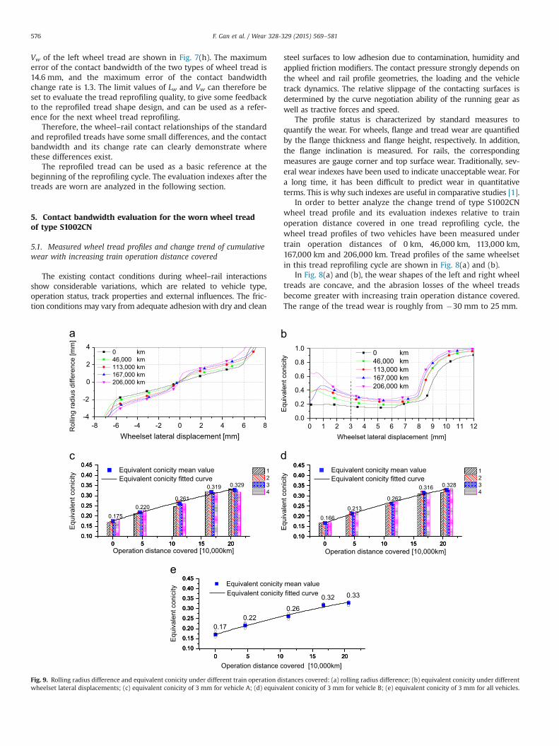
Fig. 9. Rolling radius difference and equivalent conicity under different train operation diwheelset lateral displacements; (c) equivalent conicity of 3 mm for vehicle A; (d) equiva

steel surfaces to low adhesion due to contamination, humidity andapplied friction modifiers. The contact pressure strongly depends onthe wheel and rail profile geometries, the loading and the vehicletrack dynamics. The relative slippage of the contacting surfaces isdetermined by the curve negotiation ability of the running gear aswell as tractive forces and speed.

The profile status is characterized by standard measures toquantify the wear. For wheels, flange and tread wear are quantifiedby the flange thickness and flange height, respectively. In addition,the flange inclination is measured. For rails, the correspondingmeasures are gauge corner and top surface wear. Traditionally, sev-eral wear indexes have been used to indicate unacceptable wear. Fora long time, it has been difficult to predict wear in quantitativeterms. This is why such indexes are useful in comparative studies [1].

In order to better analyze the change trend of type S1002CNwheel tread profile and its evaluation indexes relative to trainoperation distance covered in one tread reprofiling cycle, thewheel tread profiles of two vehicles have been measured undertrain operation distances of 0 km, 46,000 km, 113,000 km,167,000 km and 206,000 km. Tread profiles of the same wheelsetin this tread reprofiling cycle are shown in Fig. 8(a) and (b).

In Fig. 8(a) and (b), the wear shapes of the left and right wheeltreads are concave, and the abrasion losses of the wheel treadsbecome greater with increasing train operation distance covered.The range of the tread wear is roughly from �30 mm to 25 mm.

0 1 2 3 4 5 6 7 8 9 10 11 120.0

0.2

0.4

0.6

0.8

1.0 0 km 46,000 km 113,000 km 167,000 km 206,000 km

Equ

ival

ent c

onic

ity


0.166

0.213

0.262

0.316 0.328

0 5 10 15 200.10

0.15

0.20

0.25

0.30

0.35

0.40

0.45


1234

0 5 10 15 200.10

0.15

0.20

0.25

0.30

0.35

0.40

0.45

Equ

ival

ent c

onic

ity

Equivalent conicity mean value

0 5 10 15 200.10

0.15

0.20

0.25

0.30

0.35

0.40

0.45

Equivalent conicity fitted curve

0.260.32 0.33

15 20

overed [10,000km]15 20

mean value

15 20

fitted curve

stances covered: (a) rolling radius difference; (b) equivalent conicity under differentlent conicity of 3 mm for vehicle B; (e) equivalent conicity of 3 mm for all vehicles.

F. Gan et al. / Wear 328-329 (2015) 569–581 577

In Fig. 8(c) and (d), the position of maximum tread wear isnearly at 3 mm inside the nominal rolling circle, but the wear ofthe wheel flange is not obvious in this wheel tread reprofilingcycle. In Fig. 8(e) and (f), each vehicle has eight wheel treads. Fromthe cumulative wear changes of these two vehicles, the cumulativewears of the wheel treads at the nominal rolling circles areincreasing with train operation distance covered. In addition, thereis a linear relationship between the cumulative wear and the trainoperation distance covered, which can be seen in Fig. 8(g).

The expression of cumulative wear w with regard to trainoperation distance covered s (units of 10,000 km) can be expres-sed as follows:

w s0.02917 0.02637 (6)= + ×

In formula (6), there is a cumulative wear of 0.02917 mm at adistance of 0 km, which is due to the measurement error of theprofilometer. The cumulative wear growth rate of the wheel treadfor each 10,000 km is 0.02637 mm. The range of train operationdistance covered s is from 0 km to 206,000 km.

From the measured wheel tread profiles, only the wearappearance and the growth trend of the cumulative wear can beobtained. In order to study the contact relationship between theworn wheel tread profile and the rail surface, more results of thewheel–rail contact relationship are required.

0 km

46,000 km

113,000 km

167,000 km

206,000 km

Fig. 10. Wheel–rail contact point geometry relationships of type S1002CN wheel tread unto color in this figure, the reader is referred to the web version of this article.)

5.2. Change trend of equivalent conicity relative to train operationdistance covered

Considering the wheel axle's roll when the wheelset moveslaterally on the track, the rolling radius differences of differentwheel treads can be calculated using TPLWRSim software, and theirresults are shown in Fig. 9(a). The equivalent conicity according tostandard UIC519 is also calculated, and the results are shown inFig. 9(b)–(e).

In Fig. 9(a), the rolling radius differenceΔr increases with trainoperation distance covered, and the equivalent conicity alsoincreases in Fig. 9(c) and (d).

According to Fig. 9(e), the expression of equivalent conicitytan eφ with regard to train operation distance covered s (units of10,000 km) can be expressed as follows:

s stan 0.1708 0.00974 9.13748 10 (7)e5 2φ = + × − × ×−

Equivalent conicity is often used as an evaluation index forvehicle running stability. New wheelsets with smaller equivalentconicity have better running stability. With increasing train opera-tion distance covered, equivalent conicity constantly increases. Whenthe level of equivalent conicity reaches a certain degree, the opera-tion state of the vehicle will be unstable. Therefore, the wheel tread

der different train operation distances covered. (For interpretation of the references

F. Gan et al. / Wear 328-329 (2015) 569–581578

must be reprofiled to restore a small equivalent conicity to sustainthe stability of the vehicle.

5.3. Change trend of contact bandwidth and its change rate

TPLWRSim software can be used to calculate the wheel–railcontact point geometry relationship under different train opera-tion distances covered, and the results are shown in Fig. 10. Thenumbers above the tread wear curve are the wheelset lateraldisplacements.

In Fig. 10, the contact bandwidth increases with train operationdistance covered, when the wheelset lateral displacement is73 mm. It is important to note that the wear curve (green line) ofthe worn wheel tread in Fig. 10 is relative to the shape of thestandard wheel tread. From the shape of the wear curve aroundthe wheel tread's nominal rolling circle, the maximum range ofthe wheelset lateral displacement in the wear pit of the tread is76 mm. The lateral position distributions of the left and rightwheels tread contact points with different train operation dis-tances covered are shown in Fig. 11.

In Fig. 11(a) and (b), with increasing wheelset lateral displace-ment, the lateral position values of the worn wheel tread contactpoints are monotonically changing. In order to better display thelateral position changes of the wheel–rail contact points, three-dimensional streamline charts about the wheelset lateral dis-placement distributions on the left and right wheels tread surfacesare drawn in Fig. 11(c) and (d). The color scales and numbers inFig. 11(c) and (d) represent the wheelset lateral displacements.

Fig. 11(c) and (d) clearly shows the changes of the wheelsetlateral displacement streamlines on the left and right wheel treadsurfaces with increasing train operation distance covered. Thecontact bandwidth can be measured between the positive andnegative values of the wheelset lateral displacement streamline.

-10 -9

-8-7

-6-5

-4 -3-2 -1

01234

56

78910

0.0 5.0x104 1.0x105 1.5x105 2.0x105

-40

-30

-20

-10

0

10

20

Operation mileage [km]

Trea

d X

[mm

]

-12-10-8-6-4-2024681012

y

Contact bandwidth

12 10 8 6 4 2 0 -2 -4 -6 -8 -10 -12

-60-40-20

0204060 0 km

46,000 km 113,000 km 167,000 km 206,000 km

Trea

d X

[mm

]


wheel flange

-3

Fig. 11. Lateral position and contact bandwidth streamline charts of wheel tread contactwheel tread contact point; (b) lateral position of the right wheel tread contact point; (c)streamline chart of the right wheel tread.

For example, the contact bandwidth of the left wheel tread in thetrain operation distance covered of 50,000 km is 32.36 mm undera wheelset lateral displacement from �6 mm to 6 mm, and thecontact bandwidth of right wheel tread in the train operationdistance covered of 150,000 km is 38.8 mm. Taking the left wheeltread results in Fig. 11(c) as an example, the contact bandwidthand its change rate are calculated under different wheelset lateraldisplacements. The results are shown in Fig. 12.

In Fig. 12, the change trend of the contact bandwidth and itschange rate are almost the same as equivalent conicity (Fig. 9), andwhen the wheelset lateral displacement is from 3 mm to 6 mm,the contact bandwidth increases linearly with wheelset lateraldisplacement.

The contact bandwidths Lw of 3 mm and 6 mm and the contactbandwidth change rate Vw with regard to train operation distancecovered s (units of 10,000 km) in Fig. 12 (g) and (h) can beexpressed as follows:

⎧⎨⎪⎪

⎩⎪⎪

L s s

L s s

V s s

18.64212 1.21047 0.02502

29.37227 0.86463 0.01261

3.10344 0.20448 0.00436 (8)

w

w

w

2

2

2

3

6

3

= + × − ×

= + × − ×

= + × − ×

The contact bandwidths of real wheel treads are shown inFig. 13.

In Fig. 13(a), the measured contact bandwidth of a left wheel is40 mm, and the lateral position change range of its contact point isfrom 47 mm to 87 mm. According to formula (8), let L 40 mmw6 = ,the running distance covered of wheel tread be s 160, 500 m= ,and the equivalent conicity can be estimated as 0.304 according toformula (7). In Fig. 13(b), the measured contact bandwidth of theother left wheel is 34 mm, and the lateral position change range ofits contact point is from 49 mm to 84 mm. According to formula

10 9

8

76

5 43

2 1

0-1-2-3-4

-5 -6 -7-8-9-10

0.0 5.0x104 1.0x105 1.5x105 2.0x105

-40

-30

-20

-10

0

10

20

Operation mileage [km]

Trea

d X

[mm

]

-12-10-8-6-4-2024681012

y

Contact bandwidth

12 10 8 6 4 2 0 -2 -4 -6 -8 -10 -12

-60-40-20

0204060 0 km

46,000 km 113,000 km 167,000 km 206,000 km

Trea

d X

[mm

]


wheel flange

-3

points with different train operation distances covered: (a) lateral position of the leftcontact bandwidth streamline chart of the left wheel tread; (d) contact bandwidth

0 1 2 3 4 5 6 7 8 9 10 11 120

10203040506070

0 km 46,000 km 113,000 km 167,000 km 206,000 km

]m

m[htdi

wdna btcatnoC

Wheelset lateral displacement [mm]0 1 2 3 4 5 6 7 8 9 10 11 12

0

2

4

6

8

10 0 km 46,000 km 113,000 km 167,000 km 206,000 km

etaregnahc

htd iwd na btcat no

C Wheelset lateral displacement [mm]

0 5 10 15 200

10

20

30

40

50

60

70

0 5 10 15 200

10

20

30

40

50

60

70

0 5 10 15 200

10

20

30

40

50

60

70

0 5 10 15 200

10

20

30

40

50

60

70

30.1 34.1 38.0 41.3 42.8

18.624.3

29.4 32.2 33.6

0 5 10 15 200

10

20

30

40

50

60

7012345678

Contact bandwidth mean value (6mm) Contact bandwidth fitted curve (6mm)

0 5 10 15 200

10

20

30

40

50

60

70]m

m[htdi

wdnabtcatnoC



0 5 10 15 200

10

20

30

40

50

60

70

0 5 10 15 200

10

20

30

40

50

60

70

0 5 10 15 200

10

20

30

40

50

60

70

0 5 10 15 200

10

20

30

40

50

60

70

28.6 32.6 36.4 39.6 40.8

18.823.5

28.6 31.5 32.4

0 5 10 15 200

10

20

30

40

50

60

7012345678


0 5 10 15 200

10

20

30

40

50

60

70]m

m[htdi

wdn abtcatnoC



0 5 10 15 202

3

4

5

6

7

0 5 10 15 202

3

4

5

6

7

3.09

4.05

4.905.36 5.54

0 5 10 15 202

3

4

5

6

7

Con

tact

ban

dwid

th c

hang

e ra

te


12345678

Contact bandwidth change rate mean value Contact bandwidth change rate fitted curve

0 5 10 15 202

3

4

5

6

7

0 5 10 15 202

3

4

5

6

7

3.133.91

4.775.25 5.40

0 5 10 15 202

3

4

5

6

7

Con

tact

ban

dwid

th c

hang

e ra

te


12345678


0 3 6 9 12 15 18 21

20

30

40

50

60

70

0 3 6 9 12 15 18 21

20

30

40

50

60

70

0 3 6 9 12 15 18 21

20

30

40

50

60

70

0 3 6 9 12 15 18 21

20

30

40

50

60

70

0 3 6 9 12 15 18 21

20

30

40

50

60

70

0 3 6 9 12 15 18 21

20

30

40

50

60

70

18.723.9

29.0 31.8 33.029.3

33.437.2 40.5 41.8

Con

tact

ban

dwid

th [m

m]




0 3 6 9 12 15 18 21

3

4

5

6

7

0 3 6 9 12 15 18 21

3

4

5

6

7

0 3 6 9 12 15 18 21

3

4

5

6

7

3.1

4.0

4.85.3 5.5

Con

tact

ban

dwid

th c

hang

e ra

te



Fig. 12. Contact bandwidth and its change rate of the left wheel tread: (a) contact bandwidth; (b) contact bandwidth change rate; (c) contact bandwidth of 3 mm and 6 mmfor vehicle A; (d) contact bandwidth of 3 mm and 6 mm for vehicle B; (e) contact bandwidth change rate of 3 mm for vehicle A; (f) contact bandwidth change rate of 3 mmfor vehicle B; (g) contact bandwidth of 3 mm and 6 mm for all vehicles; (h) contact bandwidth change rate of 3 mm for all vehicles.

F. Gan et al. / Wear 328-329 (2015) 569–581 579

(8), let L 34 mmw6 = , the running distance covered of wheel tread

s 58, 500 m= , and equivalent conicity can be estimated as 0.225according to formula (7).

From the analysis results above, the contact relationship of theworn wheel tread and vehicle running stability can be evaluatedby the index of the tread cumulative wear, equivalent conicity,contact bandwidth and its change rate from different perspectives.

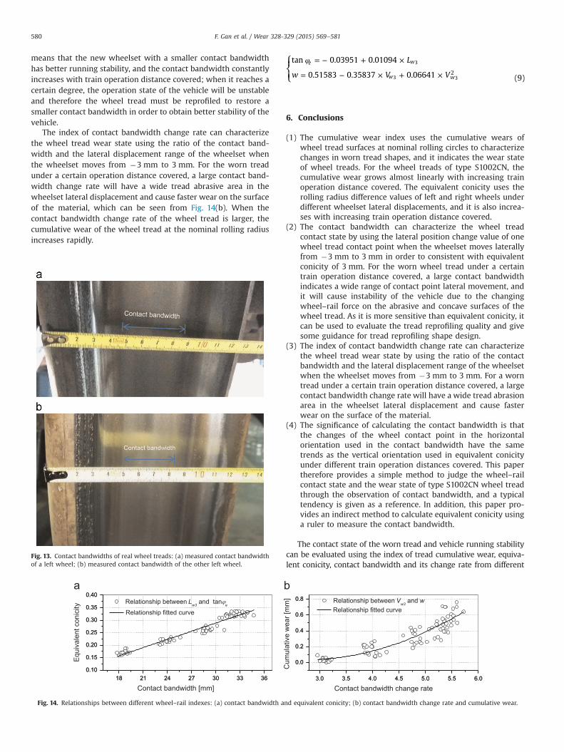
The index of contact bandwidth can characterize the wheeltread contact state using the lateral position change of one wheel

tread contact point when the wheelset moves laterally from�3 mm to 3 mm. For the worn wheel tread under a certain trainoperation distance covered, a large contact bandwidth indicates awide range of lateral movement of the wheel tread contact point,and it will cause instability of the vehicle due to the changingwheel–rail force on the abrasive and concave surface of the wheeltread. From Fig. 14(a), it can be observed that the contact band-width has a linear relationship with equivalent conicity. Therefore,it can use the same evaluation method as equivalent conicity. This

F. Gan et al. / Wear 328-329 (2015) 569–581580

means that the new wheelset with a smaller contact bandwidthhas better running stability, and the contact bandwidth constantlyincreases with train operation distance covered; when it reaches acertain degree, the operation state of the vehicle will be unstableand therefore the wheel tread must be reprofiled to restore asmaller contact bandwidth in order to obtain better stability of thevehicle.

The index of contact bandwidth change rate can characterizethe wheel tread wear state using the ratio of the contact band-width and the lateral displacement range of the wheelset whenthe wheelset moves from �3 mm to 3 mm. For the worn treadunder a certain operation distance covered, a large contact band-width change rate will have a wide tread abrasive area in thewheelset lateral displacement and cause faster wear on the surfaceof the material, which can be seen from Fig. 14(b). When thecontact bandwidth change rate of the wheel tread is larger, thecumulative wear of the wheel tread at the nominal rolling radiusincreases rapidly.

Fig. 13. Contact bandwidths of real wheel treads: (a) measured contact bandwidthof a left wheel; (b) measured contact bandwidth of the other left wheel.

18 21 24 27 30 33 360.10

0.15

0.20

0.25

0.30

0.35

0.40

18 21 24 27 30 33 360.10

0.15

0.20

0.25

0.30

0.35

0.40

Equ

ival

ent c

onic

ity

Contact bandwidth [mm]

Fig. 14. Relationships between different wheel–rail indexes: (a) contact bandwidth a

⎪

⎪

⎧⎨⎩

L

w V V

tan 0.03951 0.01094

0.51583 0.35837 0.06641 (9)

e w

w w2

3

3 3

φ = − + ×

= − × + ×

6. Conclusions

(1)

0

0

0

0

0

0

0

0

0

0

mm[rae

wev italu

muC

nd eq

The cumulative wear index uses the cumulative wears ofwheel tread surfaces at nominal rolling circles to characterizechanges in worn tread shapes, and it indicates the wear stateof wheel treads. For the wheel treads of type S1002CN, thecumulative wear grows almost linearly with increasing trainoperation distance covered. The equivalent conicity uses therolling radius difference values of left and right wheels underdifferent wheelset lateral displacements, and it is also increa-ses with increasing train operation distance covered.

(2)
The contact bandwidth can characterize the wheel treadcontact state by using the lateral position change value of onewheel tread contact point when the wheelset moves laterallyfrom �3 mm to 3 mm in order to consistent with equivalentconicity of 3 mm. For the worn wheel tread under a certaintrain operation distance covered, a large contact bandwidthindicates a wide range of contact point lateral movement, andit will cause instability of the vehicle due to the changingwheel–rail force on the abrasive and concave surfaces of thewheel tread. As it is more sensitive than equivalent conicity, itcan be used to evaluate the tread reprofiling quality and givesome guidance for tread reprofiling shape design.
(3)
The index of contact bandwidth change rate can characterizethe wheel tread wear state by using the ratio of the contactbandwidth and the lateral displacement range of the wheelsetwhen the wheelset moves from �3 mm to 3 mm. For a worntread under a certain train operation distance covered, a largecontact bandwidth change rate will have a wide tread abrasionarea in the wheelset lateral displacement and cause fasterwear on the surface of the material.
(4)
The significance of calculating the contact bandwidth is thatthe changes of the wheel contact point in the horizontalorientation used in the contact bandwidth have the sametrends as the vertical orientation used in equivalent conicityunder different train operation distances covered. This papertherefore provides a simple method to judge the wheel–railcontact state and the wear state of type S1002CN wheel treadthrough the observation of contact bandwidth, and a typicaltendency is given as a reference. In addition, this paper pro-vides an indirect method to calculate equivalent conicity usinga ruler to measure the contact bandwidth.
The contact state of the worn tread and vehicle running stabilitycan be evaluated using the index of tread cumulative wear, equiva-lent conicity, contact bandwidth and its change rate from different

3.0 3.5 4.0 4.5 5.0 5.5 6.0

.0

.2

.4

.6

.8

3.0 3.5 4.0 4.5 5.0 5.5 6.0

.0

.2

.4

.6

.8

Contact bandwidth change rate

uivalent conicity; (b) contact bandwidth change rate and cumulative wear.

F. Gan et al. / Wear 328-329 (2015) 569–581 581

perspectives. The wheel–rail contact state over some train operationdistances covered can be estimated by the change trends of thoseindexes relative to train operation distance covered. While theequivalent conicity is a parameter describing any wheel–rail contactgeometry with regard to vehicle dynamics and stability, the pre-sented indirect method to determine the equivalent conicity usingthe relationships described here is applicable only to selected railprofile shapes, track gauge, wheel profiles and back-to-back distanceof wheels, and also for certain vehicles and track conditions, parti-cularly for specific distributions of track curvatures. The simplemethod is currently only used for the wheel treads of type S1002CNand the newly built Chinese high speed railway. The limits of contactbandwidth and its change rate must be formulated with the wheeltread wear, the wheel–rail contact condition and the vehicle stabi-lity, and the adaptability for other types of wheel treads and railwaysneeds to be studied in the future.

Acknowledgments

This work was supported by the National Natural ScienceFoundation of China (Grant 51475388), the National Natural Sci-ence Foundation of China (Grant U1334206), and the projects ofChina Railway Corporation (Grant 2014J004–M, Grant 2014J012-E).

References

[1] R. Enblom, Deterioration mechanisms in the wheel–rail interface with focuson wear prediction: a literature review, Veh. Syst. Dyn. 47 (6) (2009) 661–700.

[2] X. Zhao, Z.F. Wen, H.Y. Wang, X.S. Jin, 3D transient finite element model forhigh-speed wheel–rail rolling contact and its application, Chin. J. Mech. Eng.49 (18) (2013) 1–7.

[3] X.S. Jin, J. Guo, X.B. Xiao, Z.F. Wen, Z.R. Zhou, Key scientific problems in thestudy on running safety of high speed trains, Chin. J. Eng. Mech. 26 (2) (2009)8–22.

[4] J. Pombo, J. Ambrósio, M. Silva, A new wheel–rail contact model for railwaydynamics, Veh. Syst. Dyn. 45 (2) (2007) 165–189.

[5] A. Innocenti, L. Marini, E. Meli, G. Pallini, A. Rindi, Development of a wearmodel for the analysis of complex railway networks, Wear 309 (1) (2014)174–191.

[6] Z.L. Li and J.J. Kalker, Simulation of severe wheel-rail wear, in: Proceedings ofthe 6th International Conference on Computer Aided Design, Manufacture andOperation in the Railway and Other Advanced Mass Transit Systems, 2–4September 1998, Lisbon, Portugal, pp. 393–402.

[7] I. Zobory, Prediction of wheel/rail profile wear, Veh. Syst. Dyn. (1997) 221–259.[8] O. Polach, Wheel profile design for target conicity and wide tread wear

spreading, Wear 271 (1) (2011) 195–202.[9] X.S. Jin, Z.Y. Shen, Rolling contact fatigue of wheel/rail and its advanced

research progress, J. China Railw. Soc. 23 (2) (2001) 92–108.[10] X.S. Jin, Z.S. Shen, Development of rolling contact mechanics of wheel/rail

systems, China J. Adv. Mech. 31 (1) (2001) 33–46.[11] O. Polach, Characteristic parameters of nonlinear wheel/rail contact geometry,

Veh. Syst. Dyn. 48 (S1) (2010) 19–36.[12] BS EN 14363, Railway Applications – Testing for the Acceptance of Running

Characteristics of Railway Vehicles – Testing of Running Behavior and Sta-tionary Tests, 1st ed., 2005.

[13] UIC Code 518, Testing and Approval of Railway Vehicles from the Point of Viewof their Dynamic Behavior–Safety–Track fatigue–Ride Quality, 3rd ed., 2005.

[14] UIC Code 519, Method for Determining the Equivalent Conicity, 1st ed.,December 2004.

[15] X.Q. Dong, Y.M. Wang, L.D. Wang, H.Y. Liu, G.L. Song, Research on the repro-filing strategy for the wheel tread of high-speed EMU, China Railw. Sci. 34 (1)(2013) 88–94.

[16] Q.Z. Li, S.G. Sun, L. Chen, Y.C. Zhang, A.G. Wang, Z.S. Ren, Design and dynamicsverification of economical profiled wheel tread XP 55-28, J. China Railw. Soc.35 (1) (2013) 19–24.

[17] J. Pombo, J. Ambrosio, M. Pereira, R. Lewis, R. Dwyer–Joyce, C. Ariaudo,N. Kuka, Development of a wear prediction tool for steel railway wheels usingthree alternative wear functions, Wear 271 (2011) 238–245.

[18] A. Bevan, P. Molyneux–Berry, B. Eickhoff, M. Burstow, Development and vali-dation of a wheel wear and rolling contact fatigue damage model, Wear 307(2013) 100–111.

[19] M. Ignesti, M. Malvezzi, L. Marini, E. Meli, A. Rindi, Development of a wearmodel for the prediction of wheel and rail profile evolution in railway systems,Wear 284 (2012) 1–17.

[20] W.M. Zhai, J.M. Gao, P.F. Liu, K.Y. Wang, Reducing rail side wear on heavy-haulrailway curves based on wheel–rail dynamic interaction, Veh. Syst. Dyn. 52(S1) (2014) 440–454.

[21] J. Pombo, H. Desprets, R. Verardi, J. Ambrósio, M. Pereira, C. Ariaudo, N. Kuka,Wheel wear evolution and its influence on the dynamic behaviour of railwayvehicles, in: Proceedings of the 7th EUROMECH Solid Mechanics Conference,Lisbon, Portugal, 7–11 September 2009.

[22] F. Gan, H.Y. Dai, H. Gao, L. Wei, Calculation of equivalent conicity and wheel–rail contact relationship of different railway vehicle treads, J. China Railw. Soc.35 (9) (2013) 19–24.

[23] Y. Bezin, S.D. Iwnicki, M. Cavalletti, The effect of dynamic rail roll on thewheel–rail contact conditions, Veh. Syst. Dyn. 46 (S1) (2008) 107–117.

[24] N. Burgelman, Z. Li, R. Dollevoet, A new rolling contact method applied toconformal contact and the train–turnout interaction, Wear 321 (2014) 94–105.

[25] F. Gan, H.Y. Dai, H. Gao, Calculation method of accurate wheel–rail contactrelationship of worn wheel tread, China J. Traffic Transp. Eng. 14 (3) (2014)43–51.

[26] M. Arnold, H. Netter, Apporoximation of contact geometry in the dynamicalsimulation of wheel–rail, Math. Comput. Model. Dyn. Syst. 4 (2) (1998)162–184.

[27] G. Schupp, C. Weidemann, L. Mauer, Modelling the contact between wheeland rail within multibody system simulation, Veh. Syst. Dyn. 41 (5) (2004)349–364.

[28] H. Netter, G. Schupp, W. Rulka, K. Schroeder, New aspects of contact modellingand validation within multibody system simulation of railway vehicles, Veh.Syst. Dyn. 29 (S1) (1998) 246–269.

[29] EN 15302, Railway Applications. Method for Determining the EquivalentConicity, 1st ed., February 2008.

[30] O. POLACH, Influence of wheel/rail contact geometry on the behavior of arailway vehicle at stability limit, in: Proceedings of the ENOC-2005, EindhovenUniversity of Technology, 2005, pp. 2203–2210.

[31] L. Mauer, The modular description of the wheel to rail contact within thelinear multibody formalism, in: J. Kisilowski, K. Knothe (eds.), AdvancedRailway Vehicle System Dynamics, Wydawnictwa Naukowo-Techniczne,Warsaw, 1991, pp. 205–244.

[32] S. Iwnicki (Ed.), Handbook of Railway Vehicle Dynamics, CRC Press, BocaRaton, FL, 2006.

[33] UIC Code 660, Measures to Ensure the Technical Compatibility of High-SpeedTrains, 2nd ed., August 2002.

[34] UIC Code 510-2, Trailing Stock: Wheels and Wheelsets. Conditions Concerningthe Use of Wheels of Various Diameters, 4th ed., May 2004.

[35] BS EN 13715, Railway Applications. Wheelsets and Bogies. Wheels. WheelsTread, 1st ed., March 2006.

[36] O. Miyabitaka, Research of the determination of turning allowance for wheeltread, Foreign Locomot. Rolling Stock Technol. 1 (2009) 14–18.

[37] F. Kouyuki, Wheel tread management and its planned and economic turning,Foreign Locomot. Rolling Stock Technol. (1995) 13–17.

[38] S. Zakharov, I. Goryacheva, V. Bogdanov, D. Pogorelov, I. Zharov, V. Yazykov,E. Torskaya, S. Soshenkov., Problems with wheel and rail profiles selection andoptimization, Wear 265 (9) (2008) 1266–1272.

wheel–rail wear progression of high speed train with type s1002cn wheel treads

Documents