w07 fundamental statistics chi-square

1

QUANTITATIVE RESEARCH METHODS

Week 7

Recap • Sampling • Research design • Distributions • Normal distribution theory, SDs & z-scores

Aims for the Session • Statistical significance • Overview of inferential statistical tests •  Test assumptions •  Introduction to Chi-square

- 10 min break -

•  Introduction to SPSS environment • Descriptive statistics in SPSS • Chi-square analysis in SPSS

2

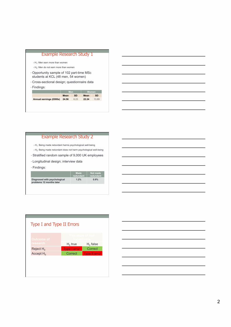
Example Research Study 1

Ø H1: Men earn more than women

Ø H0: Men do not earn more than women

• Opportunity sample of 102 part-time MSc students at KCL (48 men, 54 women)

• Cross-sectional design; questionnaire data • Findings:

Men Women Mean SD Mean SD

Annual earnings (£000s) 24.56 6.23 22.24 13.89

Example Research Study 2

Ø H1: Being made redundant harms psychological well-being

Ø H0: Being made redundant does not harm psychological well-being

• Stratified random sample of 9,000 UK employees

• Longitudinal design; interview data

• Findings: Made

redundant Not made redundant

Diagnosed with psychological problems 12 months later

1.2% 0.9%

Type I and Type II Errors

Outcome of research

True state of null hypothesis

H0 true H0 false Reject H0 Type I error Correct Accept H0 Correct Type II error

3

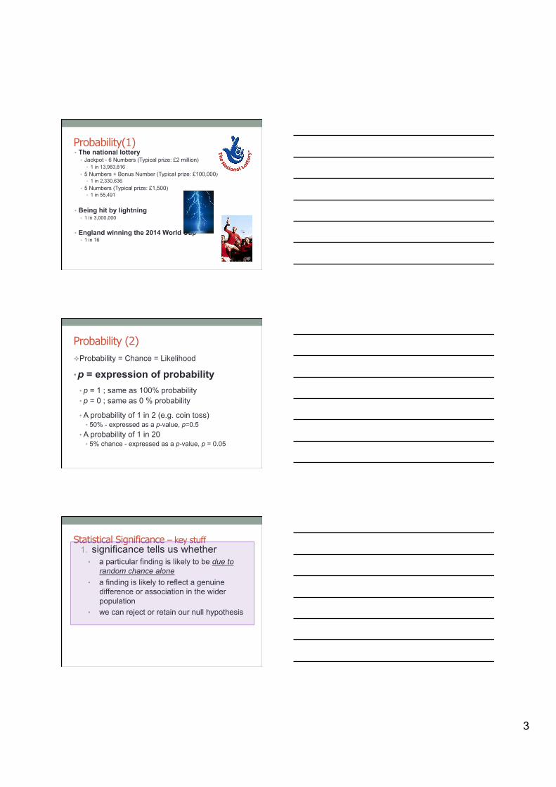
Probability(1) •  The national lottery

•  Jackpot - 6 Numbers (Typical prize: £2 million) •  1 in 13,983,816

•  5 Numbers + Bonus Number (Typical prize: £100,000) •  1 in 2,330,636

•  5 Numbers (Typical prize: £1,500) •  1 in 55,491

• Being hit by lightning •  1 in 3,000,000

• England winning the 2014 World Cup •  1 in 16

Probability (2) v Probability = Chance = Likelihood

• p = expression of probability • p = 1 ; same as 100% probability • p = 0 ; same as 0 % probability

• A probability of 1 in 2 (e.g. coin toss) • 50% - expressed as a p-value, p=0.5

• A probability of 1 in 20 • 5% chance - expressed as a p-value, p = 0.05

Statistical Significance – key stuff 1.  significance tells us whether

•  a particular finding is likely to be due to random chance alone

•  a finding is likely to reflect a genuine difference or association in the wider population

•  we can reject or retain our null hypothesis

4

Statistical Significance – key stuff 2. a p-value of 0.05 or below indicates that

a finding is significant (i.e. it is the threshold)

n  p<.05 - less than a 5% likelihood that the finding is due to random chance alone

n  lower p-values = greater significance; (p<.01 or p<.001)

3. to calculate p-values, need inferential tests

Significance and Meaningfulness • Statistical significance tells us whether, in the population,

an observed difference or association is likely to be greater than zero

Effect size = estimated size of difference or association in population

• Sometimes, the meaningfulness of a finding may be linked to a particular effect size •  So, sometimes, ‘greater than zero’ may not be enough

Salkind – core reading

Inferential Tests • Typically inferential tests examine the significance of differences and associations •  ... i.e. they produce p-values

•  Investigation of more than one variable •  bivariate or multivariate

• Many inferential tests exist • Choice of test dependent upon whether you are

examining associations or differences and on the type of data you have (i.e. nominal, ordinal, interval)

5

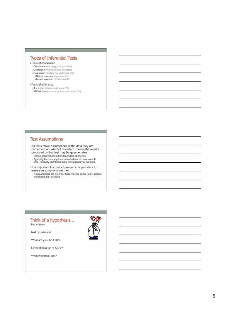
Types of Inferential Tests n Tests of association

q Chi-square (two categorical variables) q Correlation (two continuous variables) q Regression (multiple IVs and single DV)

n Multiple regression (continuous DV) n Logistic regression (dichotomous DV)

n Tests of difference q T-test (two groups, continuous DV) q ANOVA (three or more groups, continuous DV)

Test Assumptions • All tests make assumptions of the data they are carried out on, which if ‘violated’ means the results produced by that test may be questionable •  These assumptions differ depending on the test •  Typically test assumptions relate to level of data, sample

size, normally distributed data, homogeneity of variance

•  It is important to conduct pre-tests on your data to ensure assumptions are met •  If assumptions are not met, there may be some (fairly simple)

things that can be done

Think of a hypothesis... • Hypothesis:

• Null hypothesis?

• What are your IV & DV?

•  Level of data for IV & DV?

• What inferential test?

6

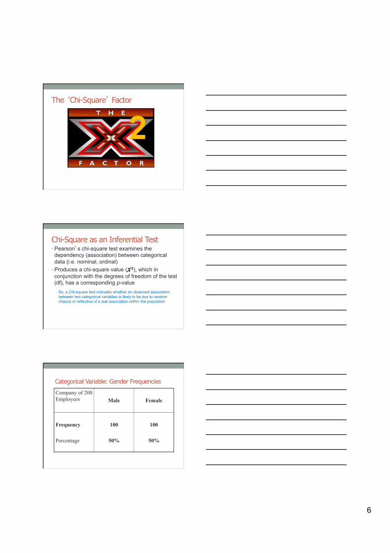
The ‘Chi-Square’ Factor

2

Chi-Square as an Inferential Test • Pearson’s chi-square test examines the dependency (association) between categorical data (i.e. nominal, ordinal)

• Produces a chi-square value (X 2), which in conjunction with the degrees of freedom of the test (df), has a corresponding p-value •  So, a Chi-square test indicates whether an observed association

between two categorical variables is likely to be due to random chance or reflective of a real association within the population

Categorical Variable: Gender Frequencies

Company of 200 Employees

Male

Female

Frequency Percentage

100

50%

100

50%

7

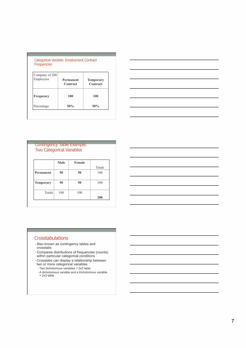
Categorical Variable: Employment Contract Frequencies

Company of 200 Employees

Permanent Contract

Temporary Contract


100

50%

100

50%

Contingency Table Example: Two Categorical Variables

Male Female Totals

Permanent 50

50

100

Temporary 50

50

100

Totals 100 100 200

Crosstabulations • Also known as contingency tables and crosstabs

• Compares distributions of frequencies (counts) within particular categorical conditions

• Crosstabs can display a relationship between two or more categorical variables •  Two dichotomous variables = 2x2 table • A dichotomous variable and a trichotomous variable

= 2x3 table

8

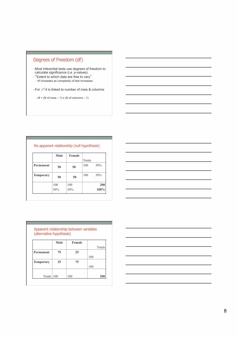
Degrees of Freedom (df)

• Most inferential tests use degrees of freedom to calculate significance (i.e. p-values)

• “Extent to which data are free to vary” •  df increases as complexity of test increases

• For X 2 it is linked to number of rows & columns

ü df = (N of rows – 1) x (N of columns – 1)

No apparent relationship (null hypothesis)

Male Female Totals

Permanent 100 50%

Temporary

100  50%

100 50%

100 50%

200 100%

50 50

50 50

Apparent relationship between variables (alternative hypothesis)

Male Female Totals

Permanent 75 25 100

Temporary 25 75 100

Totals

100

100

200

9

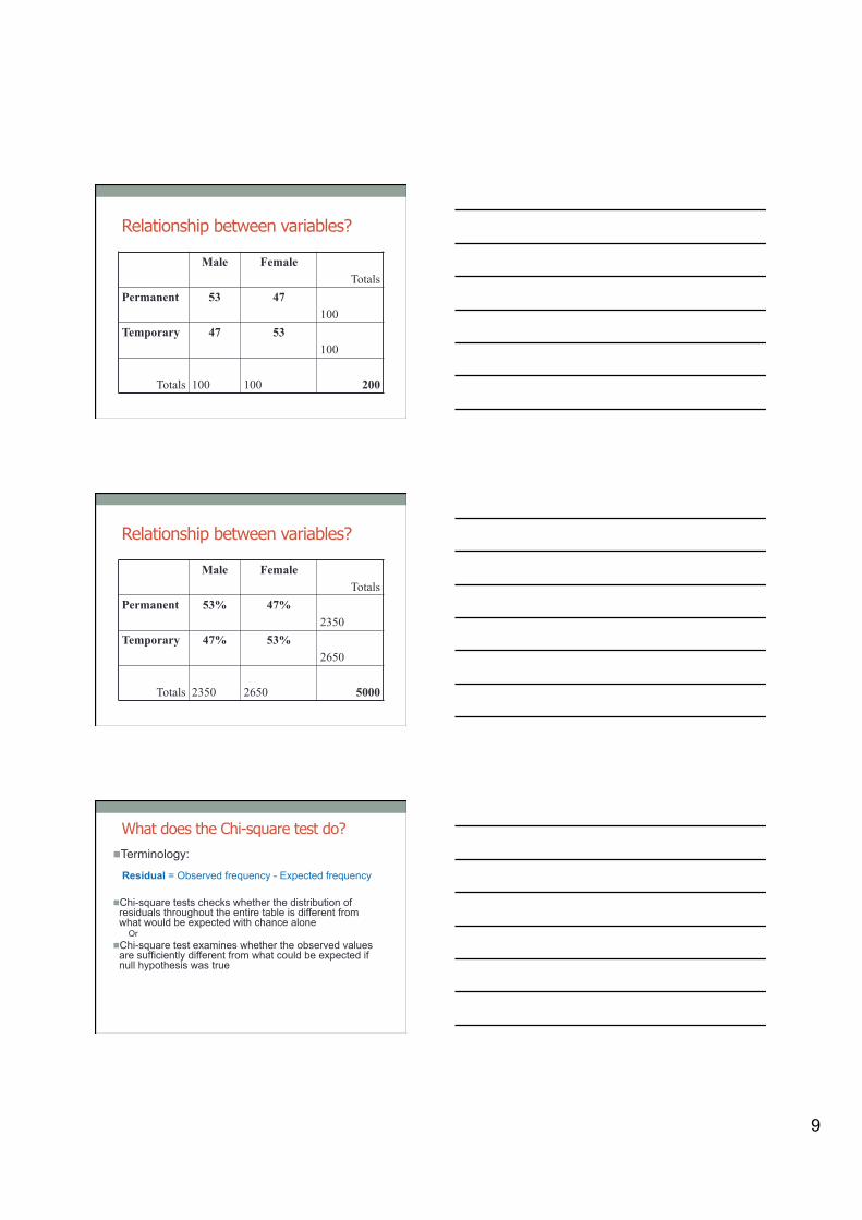
Relationship between variables?

Male Female Totals

Permanent 53 47 100

Temporary 47 53 100

Totals

100

100

200

Relationship between variables?

Male Female Totals

Permanent 53% 47% 2350

Temporary 47% 53% 2650

Totals

2350

2650

5000

What does the Chi-square test do?

n Terminology:

Residual = Observed frequency - Expected frequency

n Chi-square tests checks whether the distribution of residuals throughout the entire table is different from what would be expected with chance alone

Or n Chi-square test examines whether the observed values

are sufficiently different from what could be expected if null hypothesis was true

10

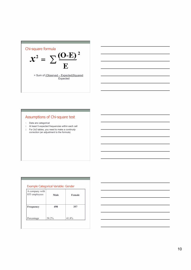
Chi-square formula

= Sum of (Observed – Expected)Squared Expected

Assumptions of Chi-square test 1.  Data are categorical 2.  At least 5 expected frequencies within each cell 3.  For 2x2 tables, you need to make a continuity

correction (an adjustment to the formula)

Example Categorical Variable: Gender

A company with 855 employees

Male

Female


498 58.2%

357 41.8%

11

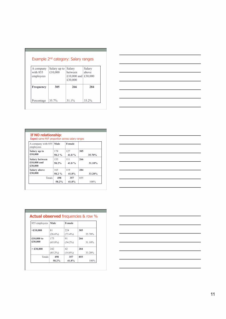
Example 2nd category: Salary ranges


Salary up to £10,000

Salary between £10,000 and £30,000

Salary above £30,000


305 35.7%

266 31.1%

284 33.2%

If NO relationship: Expect same M/F proportion across salary ranges


Male Female

Salary up to £10,000

178 58.2 %

127 41.8 %

305 35.70%

Salary between £10,000 and £30,000

155 58.2%

111 41.8 %

266 31.10%

Salary above £30,000

165 58.2 %

119 41.8%

284 33.20%

Totals 498 58.2%

357 41.8%

855 100%

Actual observed frequencies & row %

855 employees Male Female

<£10,000 81 (26.6%)

224 (73.4%)

305 35.70%

£10,000 to £30,000

175 (65.8%)

91 (34.2%)

266 31.10%

> £30,000 242 (85.2%)

42 (14.8%)

284 33.20%

Totals 498 58.2%

357 41.8%

855 100%

12

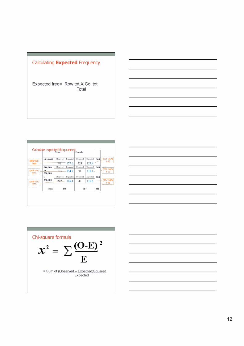
Calculating Expected Frequency

Expected freq= Row tot X Col tot Total

Male Female

<£10,000 Observed Expected Observed Expected 305 81 177.6 224 127.4

£10,000 to £30,000

Observed Expected Observed Expected 266 175 154.9 91 111.1

> £30,000

Observed Expected Observed Expected 284

242 165.4 42 118.6

Totals

498

357 855

(305*498)/855

(284*357)/855

(305*357)/855

(284*498)/855

(266*498)/855

(266*357)/855

Calculate expected frequencies

Chi-square formula

= Sum of (Observed – Expected)Squared Expected

13

Male Female


£10,000 to £30,000


> £30,000


242 165.4 42 118.6

Totals

498

357 855

(81-177.6)2

/177.6

(242-165.4)2

/165.4

(175-154.9)2

/154.9

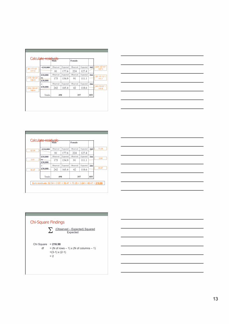
Calculate residuals

(224-127.4)2

/127.4

(91-111.1)2 /111.1

(42-118.6)2 /118.6

Male Female


£10,000 to £30,000


> £30,000


242 165.4 42 118.6

Totals

498

357 855

52.54

35.47

2.61

Calculate residuals

73.25

3.64

49.47

Sum residuals: 52.54 + 2.61 + 35.47 + 73.25 + 3.64 + 49.47 = 216.98

Chi-Square Findings

(Observed – Expected) Squared Expected

Chi Square = 216.98 df = (N of rows – 1) x (N of columns – 1) =(3-1) x (2-1) = 2

14

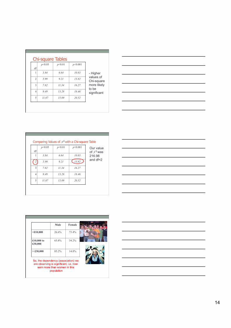
Chi-square Tables

df p<0.05 p<0.01 p<0.001

1 3.84 6.64 10.83

2 5.99 9.21 13.82

3 7.82 11.34 16.27

4 9.49 13.28 18.46

5 11.07 15.09 20.52

- Higher values of Chi-square more likely to be significant

Comparing Values of X 2 with a Chi-square Table

df

p<0.05 p<0.01 p<0.001

1 3.84 6.64 10.83

2 5.99 9.21 13.82

3 7.82 11.34 16.27

4 9.49 13.28 18.46

5 11.07 15.09 20.52

Our value of X 2 was 216.98 and df=2

Male Female

<£10,000 26.6% 73.4%

£10,000 to £30,000

65.8% 34.2%

> £30,000 85.2% 14.8%

So, the dependency (association) we are observing is significant, i.e. men

earn more than women in this population

15

SPSS • Statistical software package

•  One of many on the market

• Allows you to perform a large range of statistical analyses • Analyses can be driven either from syntax code or by

drop-down menus •  No knowledge of the mathematics underlying the analyses required

(but it may help)

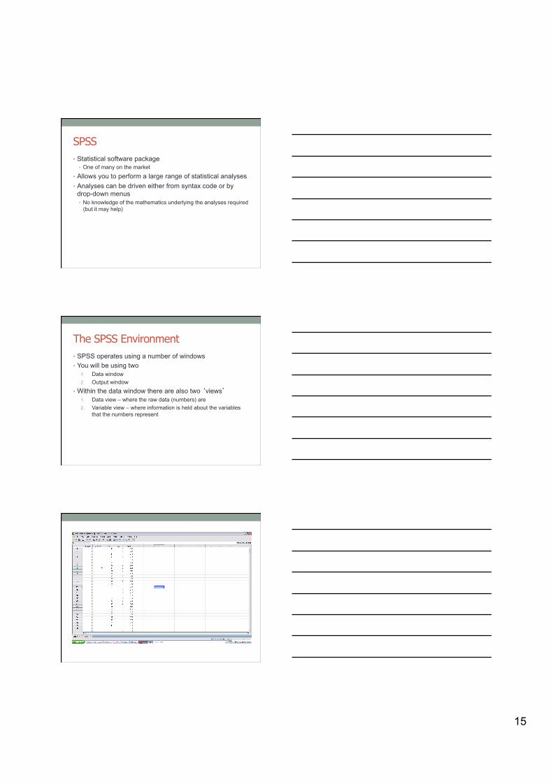
The SPSS Environment • SPSS operates using a number of windows • You will be using two

1.  Data window 2.  Output window

• Within the data window there are also two ‘views’ 1.  Data view – where the raw data (numbers) are 2.  Variable view – where information is held about the variables

that the numbers represent

Data View

16

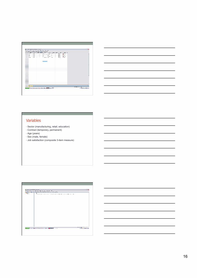
Variable View

Variables • Sector (manufacturing, retail, education) • Contract (temporary, permanent) • Age (years) • Sex (male, female) •  Job satisfaction (composite 3-item measure)

Output Window

17

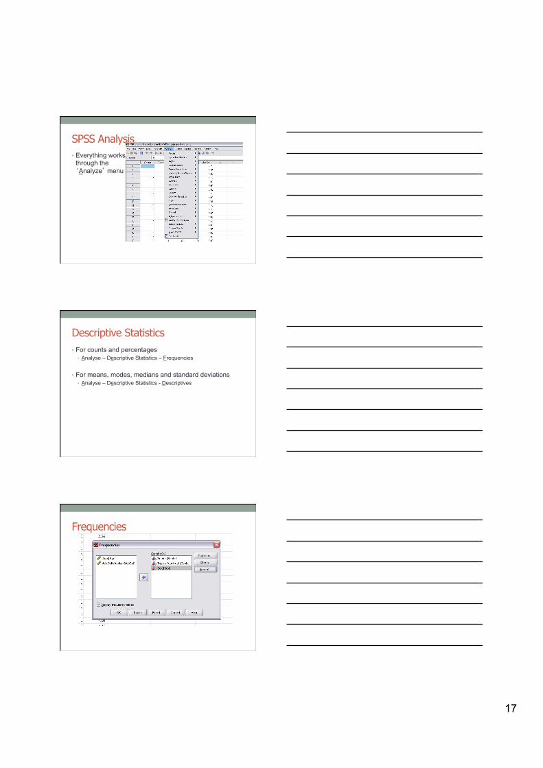
SPSS Analysis • Everything works

through the ‘Analyze’ menu

Descriptive Statistics •  For counts and percentages

•  Analyse – Descriptive Statistics – Frequencies

•  For means, modes, medians and standard deviations •  Analyse – Descriptive Statistics - Descriptives

Frequencies

18

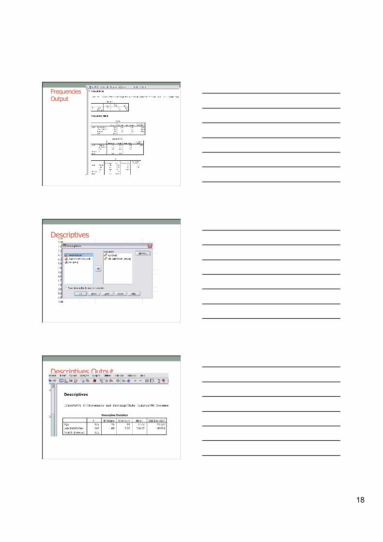
Frequencies Output

Descriptives

Descriptives Output

19

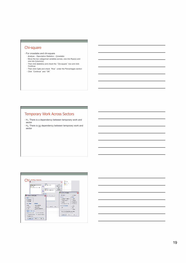
Chi-square •  For crosstabs and chi-square

•  Analyse – Descriptive Statistics – Crosstabs •  Move the two categorical variables across, one into Row(s) and

one into Column(s) •  Then click Statistics and check the ‘Chi-square’ box and click

Continue •  Then click Cells and check ‘Row’ under the Percentages section •  Click ‘Continue’ and ‘OK’

Temporary Work Across Sectors • H1: There is a dependency between temporary work and

sector • H0: There is no dependency between temporary work and

sector

Chi-square

20

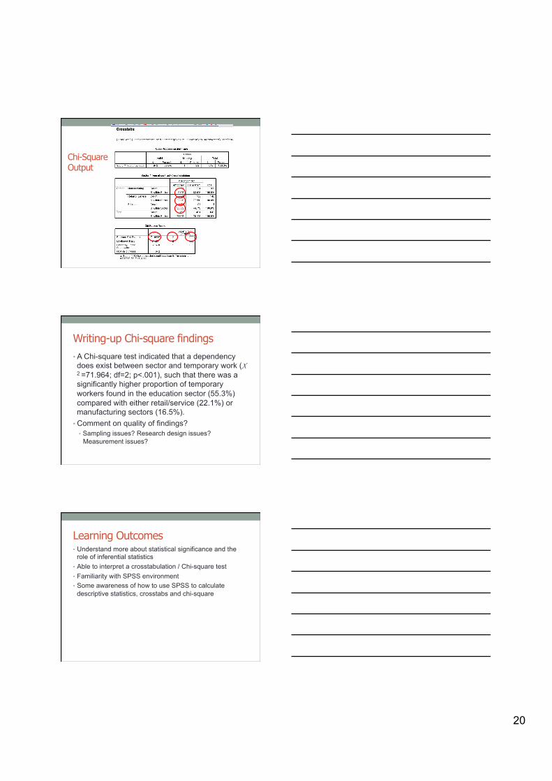
Chi-Square Output

Writing-up Chi-square findings

• A Chi-square test indicated that a dependency does exist between sector and temporary work (X 2 =71.964; df=2; p<.001), such that there was a significantly higher proportion of temporary workers found in the education sector (55.3%) compared with either retail/service (22.1%) or manufacturing sectors (16.5%).

• Comment on quality of findings? • Sampling issues? Research design issues?

Measurement issues?

Learning Outcomes • Understand more about statistical significance and the

role of inferential statistics • Able to interpret a crosstabulation / Chi-square test •  Familiarity with SPSS environment • Some awareness of how to use SPSS to calculate

descriptive statistics, crosstabs and chi-square

w07 fundamental statistics chi-square

Documents