CHI-SQUARE TEST FOR GOODNESS OF FIT TESTASSOCIATION ANDHOMOGENEITY

DR.E.S.JEEVANAND,

ASSOCIATE PROFESSOR

UNION CHRISTIAN COLLEGE. ALUVA

CHI-SQUARE TEST FOR GOODNESS OF FIT, ASSOCIATIONAND HOMOGENEITY

• Goodness of Fit Test: this test is for assessing if a particular discrete model is a good fitting model for a discrete characteristic, based on a random sample from the population.

• Test of Homogeneity: this test is for assessing if two or more populations are homogeneous (alike) with respect to the distribution of some discrete (categorical) variable.

• Test of Independence: this test helps us to assess if two discrete (categorical) variables are independent for a population, or if there is an association between the two variables.

TEST

All of these tests are based on an chi-square test statistic 𝜒 that, if the corresponding H0

is true and the assumptions hold, follows a chi-square distribution with some degrees of freedom. In general 𝜒 Test is used

• For testing significance of patterns in qualitative data

• Test statistic is based on counts that represent the number of items that fall in each category

• Test statistics measures the agreement between actual counts and expected counts. The chi-square distribution can be used to see whether or not an observed counts agree with an expected counts.

CHI-SQUARE TEST FOR GOODNESS OF FIT

The goodness of fit test involves a comparison of the observed frequency of occurrence of classes with that predicted by a theoretical model. The χ2 distribution is used for testing the goodness of fit of a set of data to a specific probability distribution. In a test of goodness of fit, the actual frequencies in a category are compared to the frequencies that theoretically would be expected to occur if the data followed the specific probability distribution of interest.

CHI-SQUARE TEST FOR GOODNESS OF FIT

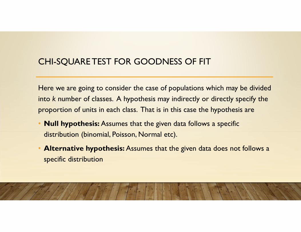
Here we are going to consider the case of populations which may be divided into k number of classes. A hypothesis may indirectly or directly specify the proportion of units in each class. That is in this case the hypothesis are

• Null hypothesis: Assumes that the given data follows a specific distribution (binomial, Poisson, Normal etc).

• Alternative hypothesis: Assumes that the given data does not follows a specific distribution

CHI-SQUARE TEST FOR GOODNESS OF FIT

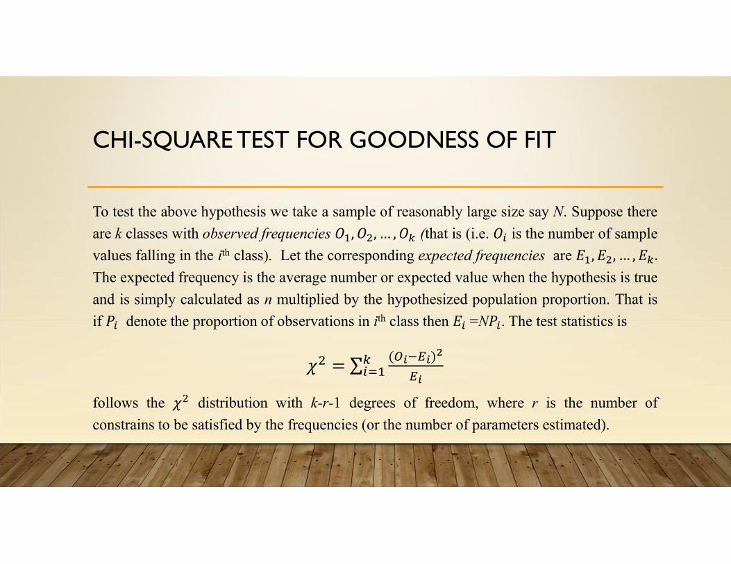
To test the above hypothesis we take a sample of reasonably large size say N. Suppose there

are k classes with observed frequencies 𝑂 , 𝑂 , … , 𝑂 (that is (i.e. 𝑂 is the number of sample

values falling in the ith class). Let the corresponding expected frequencies are 𝐸 , 𝐸 , … , 𝐸 .

The expected frequency is the average number or expected value when the hypothesis is true

and is simply calculated as n multiplied by the hypothesized population proportion. That is

if 𝑃 denote the proportion of observations in ith class then 𝐸 =N𝑃 . The test statistics is

( )

follows the 𝜒 distribution with k-r-1 degrees of freedom, where r is the number of

constrains to be satisfied by the frequencies (or the number of parameters estimated).

STEPS INVOLVED IN GOODNESS OF FIT TEST

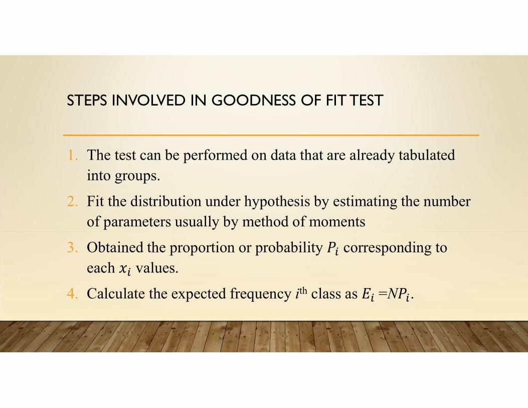
1. The test can be performed on data that are already tabulated into groups.

2. Fit the distribution under hypothesis by estimating the number of parameters usually by method of moments

3. Obtained the proportion or probability corresponding to each values.

4. Calculate the expected frequency ith class as =N .

STEPS INVOLVED IN GOODNESS OF FIT TEST

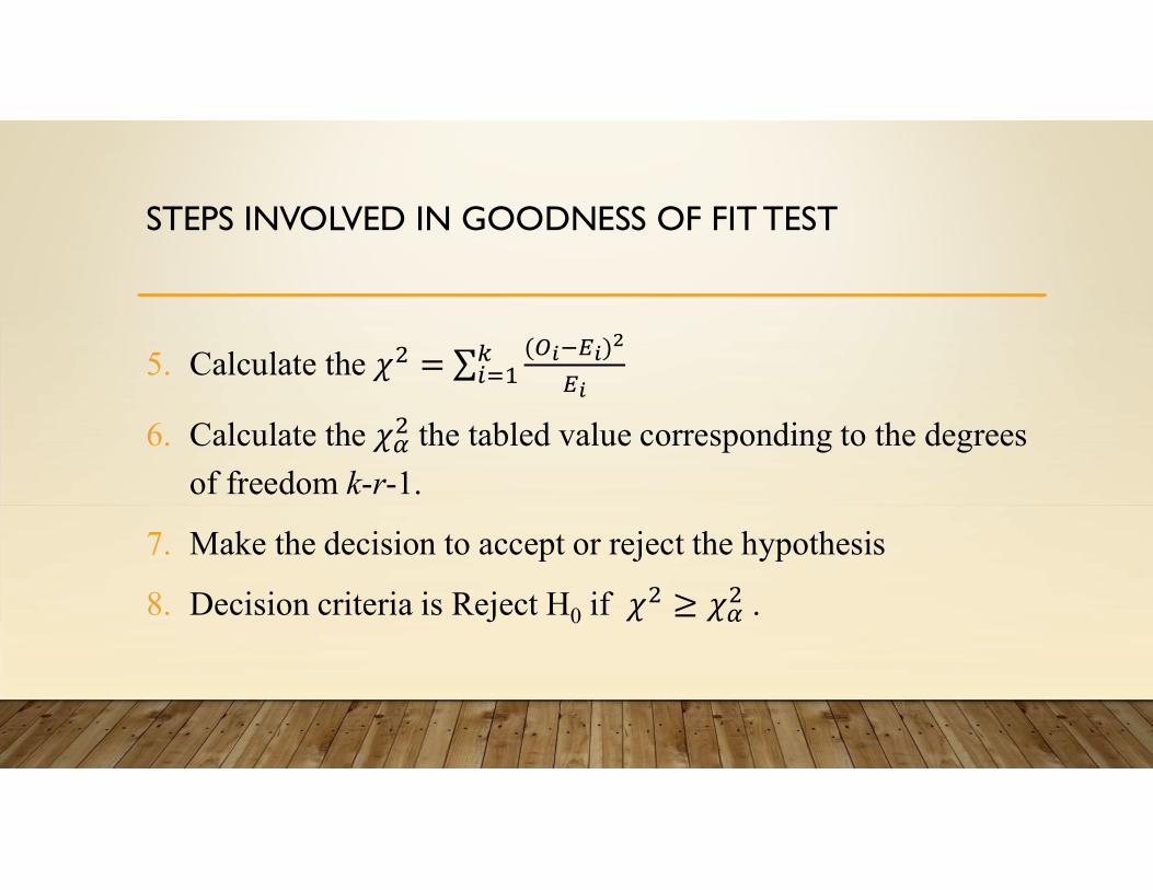
5. Calculate the ( )

6. Calculate the the tabled value corresponding to the degrees

of freedom k-r-1.

7. Make the decision to accept or reject the hypothesis

8. Decision criteria is Reject H0 if .

CHI-SQUARE TEST FOR GOODNESS OF FIT

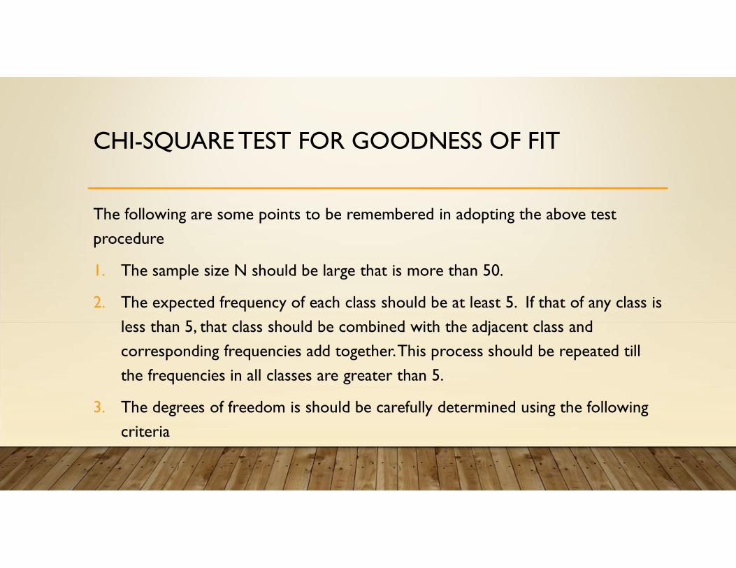
The following are some points to be remembered in adopting the above test procedure

1. The sample size N should be large that is more than 50.

2. The expected frequency of each class should be at least 5. If that of any class is less than 5, that class should be combined with the adjacent class and corresponding frequencies add together. This process should be repeated till the frequencies in all classes are greater than 5.

3. The degrees of freedom is should be carefully determined using the following criteria

CHI-SQUARE TEST FOR GOODNESS OF FIT

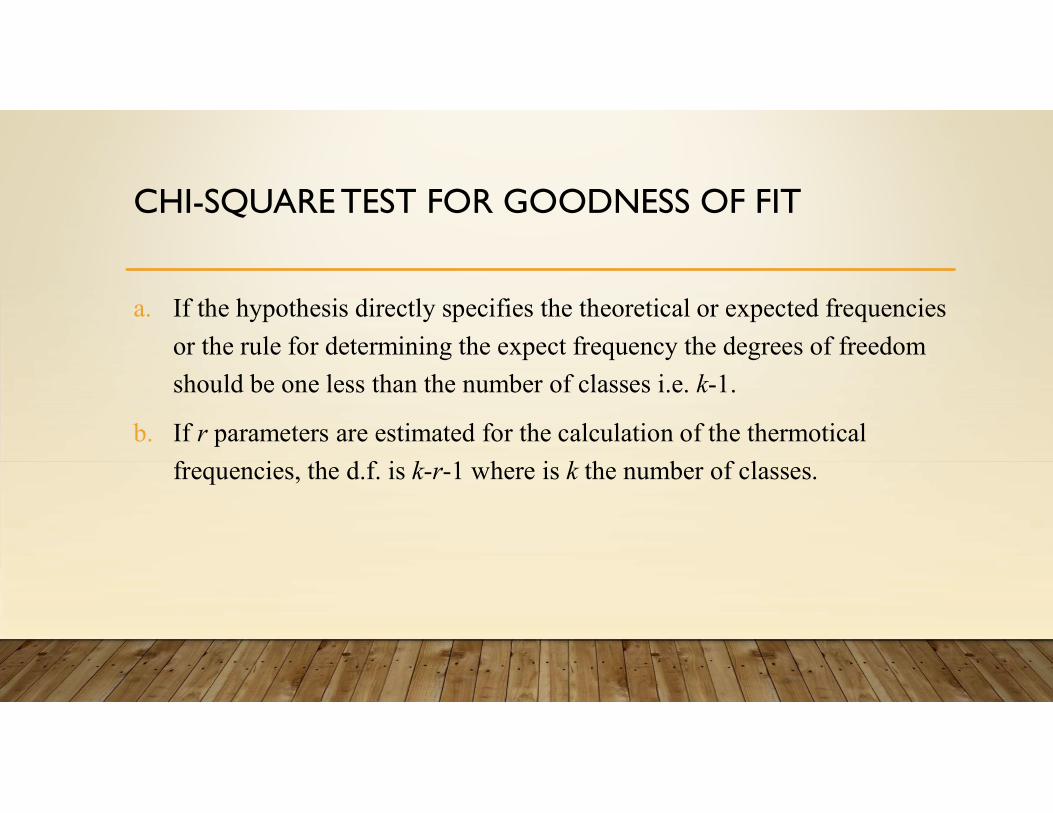
a. If the hypothesis directly specifies the theoretical or expected frequencies

or the rule for determining the expect frequency the degrees of freedom

should be one less than the number of classes i.e. k-1.

b. If r parameters are estimated for the calculation of the thermotical

frequencies, the d.f. is k-r-1 where is k the number of classes.

CHI-SQUARE TEST FOR GOODNESS OF FITTHE INTERPRETATION

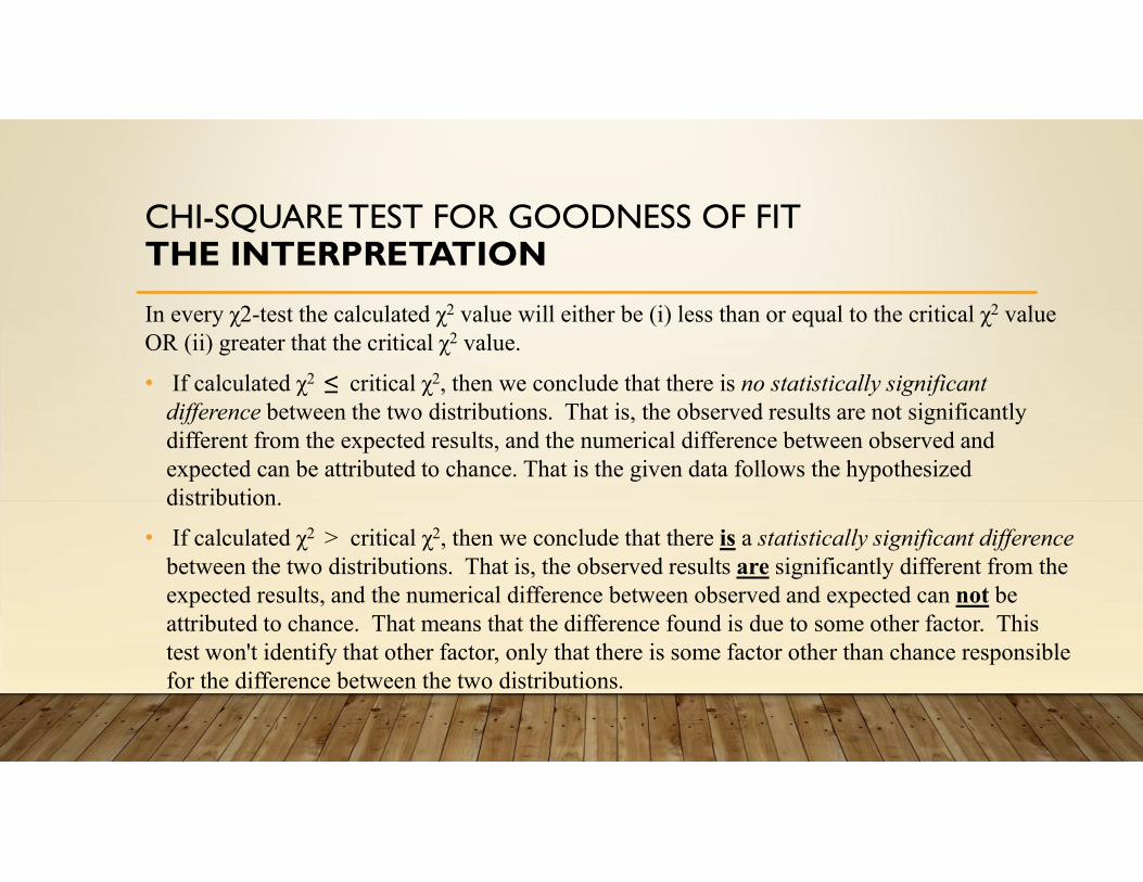
In every χ2-test the calculated χ2 value will either be (i) less than or equal to the critical χ2 value OR (ii) greater that the critical χ2 value.

• If calculated χ2 ≤ critical χ2, then we conclude that there is no statistically significant difference between the two distributions. That is, the observed results are not significantly different from the expected results, and the numerical difference between observed and expected can be attributed to chance. That is the given data follows the hypothesized distribution.

• If calculated χ2 > critical χ2, then we conclude that there is a statistically significant differencebetween the two distributions. That is, the observed results are significantly different from the expected results, and the numerical difference between observed and expected can not be attributed to chance. That means that the difference found is due to some other factor. This test won't identify that other factor, only that there is some factor other than chance responsible for the difference between the two distributions.

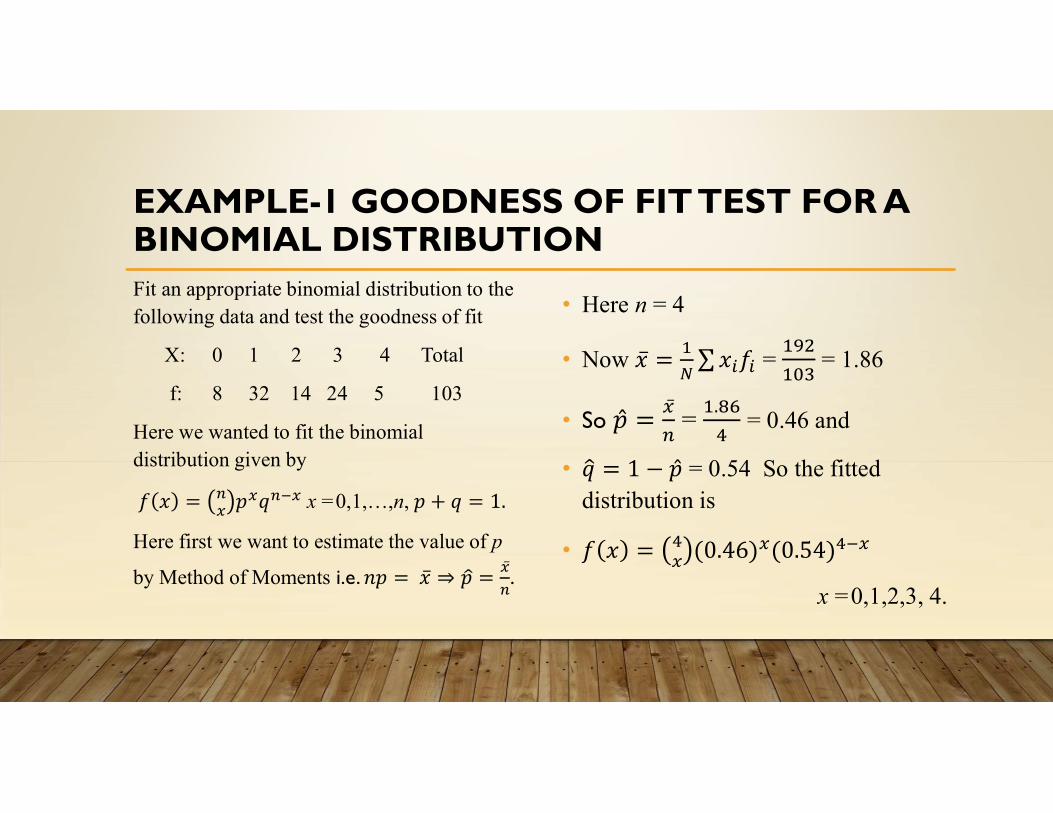
EXAMPLE-1 GOODNESS OF FIT TEST FOR A BINOMIAL DISTRIBUTIONFit an appropriate binomial distribution to the following data and test the goodness of fit

X: 0 1 2 3 4 Total

f: 8 32 14 24 5 103

Here we wanted to fit the binomial distribution given by

𝑓 𝑥 = 𝑝 𝑞 x =0,1,…,n, 𝑝 + 𝑞 = 1.

Here first we want to estimate the value of p

by Method of Moments i.e. 𝑛𝑝 = �̅� ⇒ 𝑝 =̅.

• Here n = 4

• Now = = 1.86

• So ̅=

.= 0.46 and

• = 0.54 So the fitted distribution is

•

x =0,1,2,3, 4.

EXAMPLE-1 GOODNESS OF FIT TEST FOR A BINOMIAL DISTRIBUTION

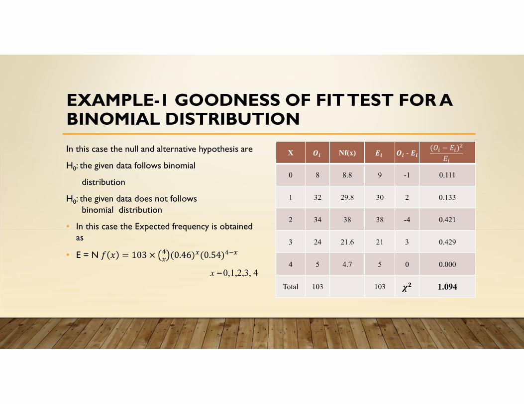
In this case the null and alternative hypothesis are

H0: the given data follows binomial

distribution

H0: the given data does not follows binomial distribution

• In this case the Expected frequency is obtained as

• E = N 𝑓 𝑥 = 103 × (0.46) (0.54)

x =0,1,2,3, 4

X 𝑶𝒊 Nf(x) 𝑬𝒊 𝑶𝒊 - 𝑬𝒊(𝑂 − 𝐸 )

𝐸

0 8 8.8 9 -1 0.111

1 32 29.8 30 2 0.133

2 34 38 38 -4 0.421

3 24 21.6 21 3 0.429

4 5 4.7 5 0 0.000

Total 103 103 𝝌𝟐 1.094

EXAMPLE-1 GOODNESS OF FIT TEST FOR A BINOMIAL DISTRIBUTION

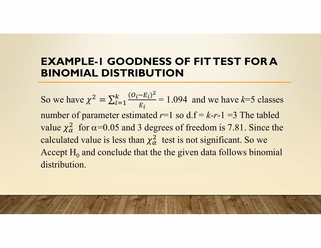
So we have ( )

= 1.094 and we have k=5 classes

number of parameter estimated r=1 so d.f = k-r-1 =3 The tabled value for =0.05 and 3 degrees of freedom is 7.81. Since the calculated value is less than test is not significant. So we Accept H0 and conclude that the the given data follows binomial distribution.

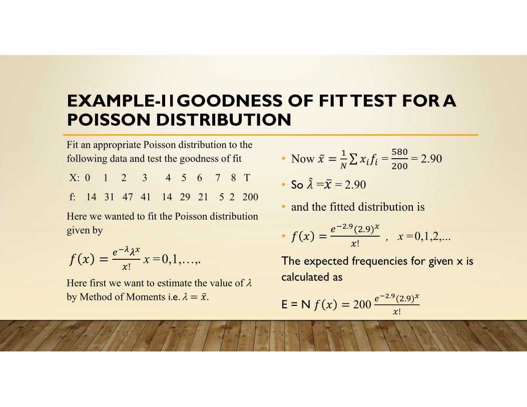
EXAMPLE-I1GOODNESS OF FIT TEST FOR A POISSON DISTRIBUTIONFit an appropriate Poisson distribution to the following data and test the goodness of fit

X: 0 1 2 3 4 5 6 7 8 T

f: 14 31 47 41 14 29 21 5 2 200

Here we wanted to fit the Poisson distribution given by

!x =0,1,…,

Here first we want to estimate the value of by Method of Moments i.e. = �̅�.

• Now = = 2.90

• So = = 2.90

• and the fitted distribution is

•. ( . )

!, x =0,1,2,...

The expected frequencies for given x is calculated as

E = N 200 . ( . )

!

EXAMPLE-I1GOODNESS OF FIT TEST FOR A POISSON DISTRIBUTION

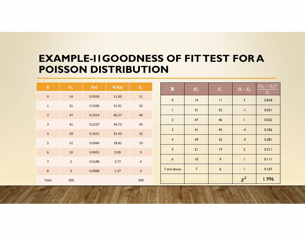
X 𝑶𝒊 f(x) N f(x) 𝑬𝒊

0 14 0.0550 11.00 11

1 31 0.1596 31.91 32

2 47 0.2314 46.27 46

3 41 0.2237 44.73 45

4 29 0.1622 32.43 32

5 21 0.0940 18.81 19

6 10 0.0455 9.09 9

7 5 0.0188 3.77 4

8 2 0.0068 1.37 2

Total 200 200

X 𝑶𝒊 𝑬𝒊 𝑶𝒊 - 𝑬𝒊(𝑂 − 𝐸 )

𝐸

0 14 11 3 0.818

1 31 32 -1 0.031

2 47 46 1 0.022

3 41 45 -4 0.356

4 29 32 -3 0.281

5 21 19 2 0.211

6 10 9 1 0.111

7 and above 7 6 1 0.167

𝝌𝟐 1.996

EXAMPLE-I1GOODNESS OF FIT TEST FOR A POISSON DISTRIBUTION

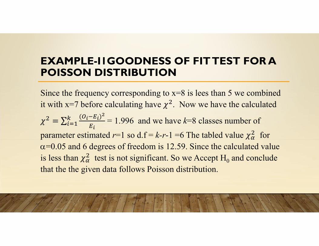
Since the frequency corresponding to x=8 is lees than 5 we combined it with x=7 before calculating have . Now we have the calculated

( )= 1.996 and we have k=8 classes number of

parameter estimated r=1 so d.f = k-r-1 =6 The tabled value for =0.05 and 6 degrees of freedom is 12.59. Since the calculated value is less than test is not significant. So we Accept H0 and conclude that the the given data follows Poisson distribution.

EXAMPLE-I1I

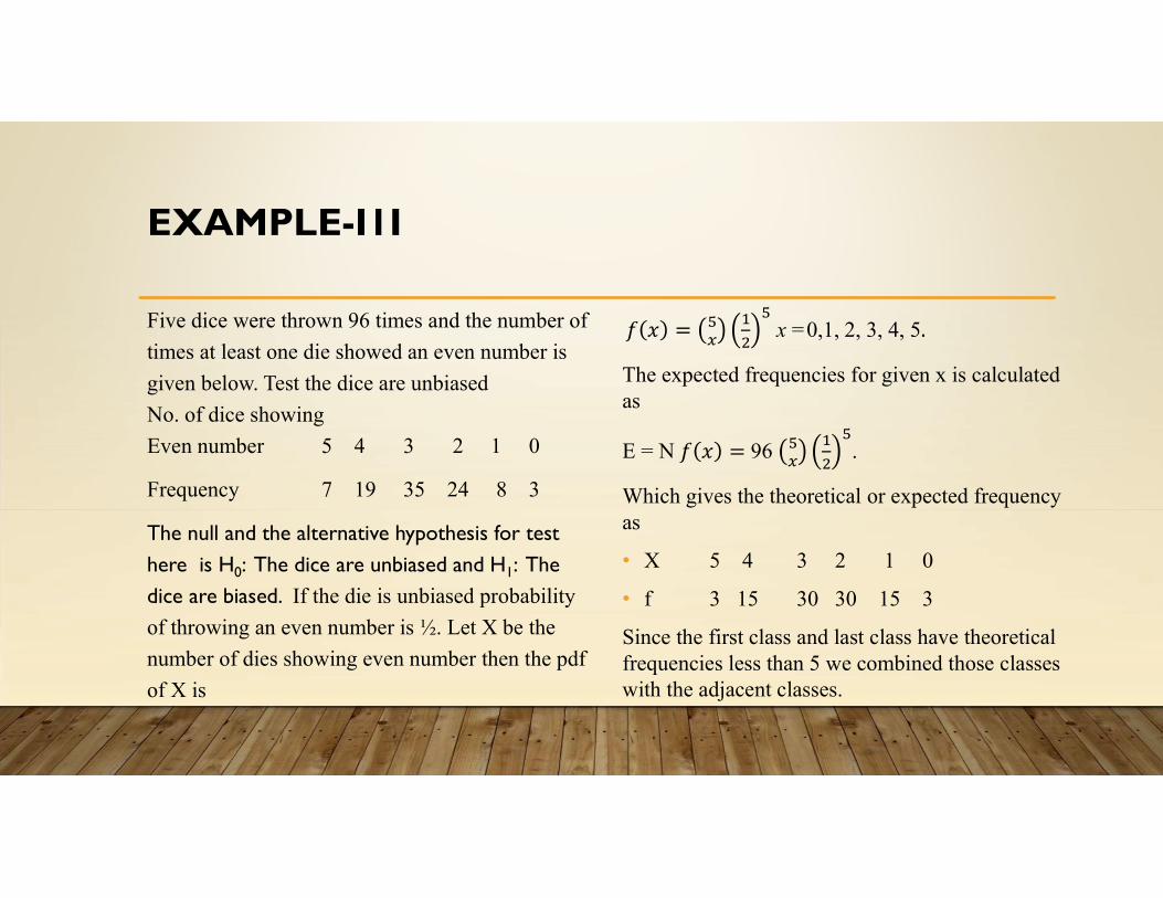
Five dice were thrown 96 times and the number of

times at least one die showed an even number is

given below. Test the dice are unbiased

No. of dice showing

Even number 5 4 3 2 1 0

Frequency 7 19 35 24 8 3

The null and the alternative hypothesis for test here is H0: The dice are unbiased and H1: The dice are biased. If the die is unbiased probability

of throwing an even number is ½. Let X be the

number of dies showing even number then the pdf

of X is

𝑓 𝑥 = x =0,1, 2, 3, 4, 5.

The expected frequencies for given x is calculated as

E = N 𝑓 𝑥 = 96 .

Which gives the theoretical or expected frequency as

• X 5 4 3 2 1 0

• f 3 15 30 30 15 3

Since the first class and last class have theoretical frequencies less than 5 we combined those classes with the adjacent classes.

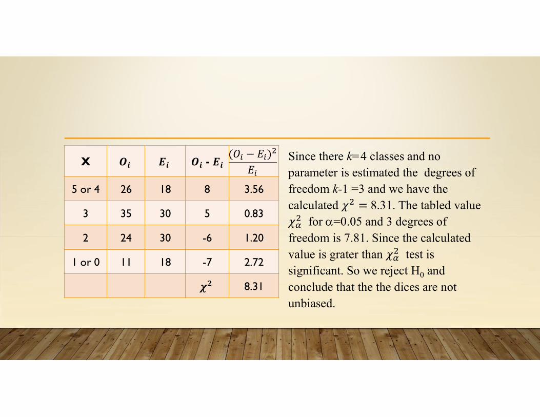
X 𝑶𝒊 𝑬𝒊 𝑶𝒊 - 𝑬𝒊(𝑂 − 𝐸 )

𝐸

5 or 4 26 18 8 3.56

3 35 30 5 0.83

2 24 30 -6 1.20

1 or 0 11 18 -7 2.72

𝝌𝟐 8.31

Since there k=4 classes and no parameter is estimated the degrees of freedom k-1 =3 and we have the calculated 8.31. The tabled value

for =0.05 and 3 degrees of freedom is 7.81. Since the calculated value is grater than test is significant. So we reject H0 and conclude that the the dices are not unbiased.

You can wait for next presentation for chi square test for Association!

Contact details esjmaths@gmail.com

9847915101, 8089684892

The End