Voting Systems and Automated Reasoning:the QBFEVAL Case Study

Massimo Narizzano and Luca Pulina and Armando Tacchella1

Abstract

Systems competitions play a fundamental role in the advancement of the state ofthe art in several automated reasoning fields. The goal of such events is to answerthe question: “Which system should I buy?”. Usually the answer comes as thebyproduct of a ranking obtained by considering a pool of problem instances andthen aggregating the performances of the systems on each member of the pool. Inthis paper, we consider voting systems as an alternative to other procedures whichare well established in automated reasoning contests. Our research is aimed tocompare methods that are customary in the context of social choice, with meth-ods that are targeted to artificial settings, including a new hybrid method that weintroduce. Our analysis is empirical, in that we compare the aggregation proce-dures by computing measures which should account for their effectiveness usingthe data from the 2005 evaluation of quantified Boolean formulas solvers that weorganized. The results of our experiments give useful indications about the rela-tive strengths and weaknesses of the procedures under test, and allow us to inferalso some conclusions that are independent of the specific procedure adopted.

1 Introduction

Systems competitions play a fundamental role in the advancement of the state of theart in several automated reasoning fields. A non-exhaustive list of such events in-cludes the CADE ATP System Competition (CASC) [1] for theorem provers in firstorder logic, the SAT Competition [2] for propositional satisfiability solvers, the In-ternational Planning Competition (see, e.g., [3]) for symbolic planners, the CP Com-petition (see, e.g., [4]) for constraint programming systems, the Satisfiability ModuloTheories (SMT) Competition (see, e.g., [5]) for SMT solvers, and the evaluation ofquantified Boolean formulas solvers (QBFEVAL, see [6, 7, 8] for previous reports).The main purpose of the above events is to designate a winner, i.e., to answer thequestion: “Which system should I buy?”. Even if such perspective can be limiting,and the results of automated reasoning systems competitions may provide less insightthan controlled experiments in the spirit of [9], there is a general agreement that com-petitions raise interest in the community and they help to set research challenges fordevelopers and assess the current technological frontier for users. The usual way todesignate a winner in competitions is to compute a ranking obtained by consideringa pool of problem instances and then aggregating the performances of the systems oneach member of the pool. While the definition of performances can encompass many

1The authors wish to thank the Italian Ministry of University and Research (MIUR) for its financialsupport, the anonymous reviewers who helped us to improve the quality of the paper, and Elena Seghezzafor making some relevant references available to us.

aspects of a system, usually it is the capability of giving a sound solution to a highnumber of problems in a relatively short time that matters most. Therefore, one ofthe issues that occurred to us as organizers of QBFEVAL, relates to the proceduresused to compute the final ranking of the solvers, i.e., we had to answer the question“Which aggregation procedure is best?”. Indeed, even if the final rankings cannot beinterpreted as absolute measures of merit, they should at least represent the relativestrength of a system with respect to the other competitors based on the difficulty of theproblem instances used in the contest.

Our analysis of aggregation procedures considers three voting systems, namelyBorda’s method [10], range voting [11] and Schulze’s method [12], as an alterna-tive to methods which are well estabished in automated reasoning contests, namelyCASC [1], the SAT competitions [2], and QBFEVAL [13] (before 2006). We adaptedvoting systems to the artificial setting of systems competition by considering the sys-tems as candidates and the problem instances as voters. Each instance casts its voteon the systems in such a way that systems with the best performances on the instancewill be preferred over other candidates. The individual preferences are aggregated toobtain a collective choice that determines the winner of the contest. Our motivation toinvestigate methods which are customary in the context of social choice by applyingthem to the artificial setting of systems competitions is twofold. First, although votingsystems do not enjoy a great popularity in automated reasoning systems contests (oneexception is Robocup [14] using Borda’s method), there is a substantial amount of lit-erature in social choice (see, e.g., [15]) that deals with the problem of identifying andformalizing appropriate methods of aggregation in specific domains. Second, votingcan be seen as a way to “infer the candidates’ absolute goodness based on the voters’noisy signals, i.e., their votes.” [16]. Therefore, the use of voting systems as aggrega-tion procedures could pave the way to extracting hints about the absolute value of asystem from the results of a contest.

In the paper, we also propose a new procedure called YASM (“Yet Another Scor-ing Method”)2 that we selected as an aggregation procedure for QBFEVAL’06. YASMis an hybrid between a voting system and traditional aggregation procedures used inautomated reasoning contests. Our results show that YASM provides a good compro-mise when considering some measures that should quantify desirable properties of theaggregation procedures. In particular, the measures we propose account for:

• the degree of fidelity of the procedures, i.e., given a synthesized set of raw data,evaluate whether a procedure distorts the results;

• the degree of stability of each procedure with respect to perturbations(i) in thesize of the test set,(ii) in the amount of resources available (CPU time), and(iii) in the quality of the test-set;

• the representativeness of each procedure with respect to the state of the art ex-pressed by the competitors.

2The terminology “scoring method” is somewhat inappropriate in the context of social choice, as itrecalls a positional scoring procedure such as Borda’s method and range voting; we decided to keep theoriginal terminology for consistency across the previous works [17, 18, 21].

We compute the above measures using part of the results from QBFEVAL’05 [8]. Inparticular, the results of our experiments give useful indications about the relativestrengths and weaknesses of the aggregation procedures, and allow us to infer alsosome conclusions that are independent of the specific method adopted.

This paper builds on and extends previous work by one of the authors [17]. First,the version of YASM that we present here improves on the one presented in [17]. Inparticular, the new YASM is simpler and more effective when compared to the old one.Moreover, the comparison of aggregation procedures is broadened by the addition ofnew effectiveness measures (fidelity, see Section 4), and an improved definition ofState-Of-The-Art (SOTA) relevance (see Section 4).

The paper is structured as follows. In Section 2 we introduce the case study ofQBFEVAL’05 [8], and we introduce the state of the art aggregation procedures. InSection 3 we introduce our new aggregation procedure, and then we compare it withother methods in Section 4 using several effectiveness measures. We conclude thepaper in Section 5 with a discussion about the presented results.

2 Preliminaries

2.1 QBFEVAL’05

QBFEVAL’05 [8] is the third in a series of non-competitive events that precededQBFEVAL’06. QBFEVAL’05 accounted for 13 competitors, 553 quantified Booleanformulas (QBFs) and three QBF generators submitted. The test set was assembledusing a selection of 3191 QBFs obtained considering the submissions and the in-stances archived in QBFLIB [19]. The results of QBFEVAL’05 can be listed in atable RUNS comprised of four attributes (column names):SOLVER, INSTANCE, RE-SULT, and CPUTIME. The attributesSOLVER and INSTANCE report which solver isrun on which instance.RESULT is a four-valued attribute:SAT, i.e., the instance wasfound satisfiable by the solver,UNSAT, i.e., the instance was found unsatisfiable by thesolver,TIME, i.e., the solver exceeded a given time limit without solving the instance(900 seconds in QBFEVAL’05), andFAIL , i.e., the solver aborted for some reason(e.g., a run-time error, an inherent limitation of the solver, or any other reason beyondour control). Finally,CPUTIME reports the CPU time spent by the solver on the giveninstance, in seconds. In the analysis herewith presented we used a subset of QBFE-VAL’05 RUNS table, including only the solvers that, as far as we know, work correctly(the solvers of the second stage of the evaluation) and the QBFs coming from classesof instances having fixed structure (see [8] for more details). Under these assumptions,RUNS table reduces to 4408 entries, one order of magnitude less than the original one.This choice allows us to disregard correctness issues, to reduce considerably the over-head of the computations required for our analysis, and, at the same time, maintain asignificant number of runs. The aggregation procedures that we evaluate, the measuresthat we compute and the results that we obtain, are based on the assumption that atable identical to RUNS as described above is the only input required by a procedure.As a consequence, the aggregation procedures (and thus our analysis) do not take into

account(i) memory consumption,(ii) correctness of the solution, and(iii) “quality”of the solution.

2.2 State of the art aggregation procedures

In the following we describe in some details the state of the art aggregation proceduresused in our analysis. For each method we describe only those features that are relevantfor our purposes. Further details can be found in the references provided.

CASC [1] Using CASC methodology, the solvers are ranked according to the num-ber of problems solved, i.e., the number of timesRESULT is eitherSAT or UNSAT.Under this procedure, solverA is better than solverB, if and only if A is able to solveat least one problem more thanB within the time limit. In case of a tie, the solver far-ing the lowest average onCPUTIME fields over the problems solved is the one whichranks first.

QBF evaluation [13] QBFEVAL methodology is the same as CASC, except for thetie-breaking rule, which is based on the sum ofCPUTIME fields over the problemssolved.

SAT competition [2] The last SAT competition uses apurse-based method, i.e., themeasure of effectiveness of a solver on a given instance is obtained by adding up threepurses:

• the solution purse, which is divided equally among all solvers that solve theproblem;

• the speed purse, which is divided unequally among all the competitors that solvethe problem, first by computing the speed factorFs,i of a solvers on a probleminstancei:

Fs,i =k

1 + Ts,i(1)

wherek is an arbitrary scaling factor (we setk = 104 according to [20]), andTs,i is the time spent bys to solvei; then by computing the speed awardAs,i,i.e., the portion of speed purse awarded to the solvers on the instancei:

As,i =Pi · Fs,i∑

r Fr,i(2)

wherer ranges over the solvers, andPi is the total amount of the speed pursefor the instancei.

• the series purse, which is divided equally among all solvers that solve at leastone problem in a given series (a series is a family of instances that are somehowrelated, e.g., different QBF encodings for some problem in a given domain).

The overall ranking of the solvers under this method is obtained by considering thesum of the purses obtained on each instance, and the winner of the contest is the solverwith the highest sum.

Borda’s method [10] Suppose thatn solvers (candidates) andm instances (voters)are involved in the contest. Consider the sorted list of solvers obtained for each in-stance by considering the value of theCPUTIME field in ascending order. Letps,i be theposition of a solvers (1 ≤ s ≤ n) in the list associated with instancei (1 ≤ i ≤ m).According to Borda’s method, each voter’s ballot consists of a vector of individualscores given to candidates, where the scoreSs,i of solvers on instancei is simplySs,i = n − ps,i. In cases of time limit attainment or failure, we defaultSs,i to 0. Thescore of a candidate, given the individual preferences, is justSs =

∑i Ss,i, and the

winner is the solver with the highest score.

Range voting [11] Again, suppose thatn solvers andm instance are involved in thecontest andps,i is obtained as described above for Borda’s method. We let the scoreSs,i of solvers on instancei be the quantityarn−ps,i , i.e., we use a positional scoringrule following a geometric progression with a common ratior = 2 and a scale factora = 1. We consider failures and time limit attainments in the same way (we call thisthe failure-as-time-limit model in [21]), and thus we assume that all the voters expressan opinion about all the solvers. The overall score of a candidate is againSs =

∑i Ss,i

and the candidate with the highest score wins the election.

Schulze’s method We denote as such an extension of the method described in Ap-pendix 3 of [12]. Since Schulze’s method is meant to compute a single overall winner,we extended the method according to Schulze’s suggestions [22] in order to make itcapable of generating an overall ranking.

3 YASM: Yet Another Scoring Method (Revisited)

While the aggregation procedures used in CASC and QBF evaluations are straight-forward, they do not take into account some aspects that are indeed considered bythe purse-based method used in the last SAT competition. On the other hand, thepurse-based method used in SAT requires some oracle to assign purses to the probleminstances, so the results can be influenced heavily by the oracle. In [17] a first ver-sion of YASM was introduced as an attempt to combine the two approaches: a richmethod like the purse-based one, but using the data obtained from the runs only. Asreported in [17], YASM featured a somewhat complex calculation, yielding unsatisfac-tory results, particularly in the comparison with the final ranking produced by votingsystems. Here we revise the original version of YASM to make its computation sim-pler, and to improve its performance using ideas borrowed from voting systems. Fromhere on, we call YASMv2 the revised version, and YASM the original one presentedin [17]. YASMv2 requires a preliminary classification whereby a hardness degreeHi

is assigned to each problem instancei using the same equation as in CASC [1] (andYASM):

Hi = 1− Si

St(3)

CASC QBF SAT YASM YASMv2 Borda r.v. SchulzeCASC – 1 0.71 0.86 0.79 0.86 0.71 0.86QBF – 0.71 0.86 0.79 0.86 0.71 0.86SAT – 0.86 0.86 0.71 0.71 0.71YASM – 0.86 0.71 0.71 0.71YASMv2 – 0.86 0.86 0.86Borda – 0.86 1r. v. – 0.86Schulze –

Table 1: Homogeneity of aggregation procedures.

whereSi is the number of solvers that solvedi, andSt is the total number ofparticipants to the contest. Considering equation (3), we notice that0 ≤ Hi ≤ 1,whereHi = 0 means thati is relatively easy, whileHi = 1 means thati is relativelyhard. We can then compute the measure of effectivenessSs,i of a solvers on a giveninstancei (this definition changes with respect to YASM):

Ss,i = ks,i · (1 + Hi) ·L− Ts,i

L−Mi(4)

whereL is the time limit,Ts,i is the CPU time used up bys to solvei (Ts,i ≤ L),andMi = mins{Ts,i}, i.e.,Mi is the time spent on the instancei by theSOTA solverdefined in [8] to be the ideal solver that always fares the best time among all the par-ticipants. The hybridization with voting systems comes into play with the coefficientks,i which is computed as follows. Suppose thatn solvers are participating to the con-test. Each instance ranks the solvers in ascending order considering the value of theCPUTIME field. Let ps,i be the position of a solvers in the ranking associated withinstancei (1 ≤ ps,i ≤ n), thenks,i = n − ps,i. In case of time limit attainment andfailure, we defaultks,i to 0, and thus alsoSs,i is 0. The overall ranking of the solversis computed by considering the valuesSs =

∑i Ss,i for all 1 ≤ s ≤ n, and the solver

with the highest sum wins.We can see from equation (4) that in YASMv2 the effectiveness of a solver on a

given instance is influenced by three factors, namely(i) a Borda-like positional weight(ks,i), (ii) the relative hardness of the instance (1 + Hi), and(iii) the relative speedof the solver with respect to the fastest solver on the instance (L−Ts,i

L−Mi). Intuitively,

coefficient(ii) rewards the solvers that are able to solve hard instances, while(iii)rewards the solvers that are faster than other competitors. The coefficientks,i has beenadded to stabilize the final ranking and make it less sensitive to an initial bias in thetest set. As we show in the next Section, this combination allows YASMv2 to reachthe best compromise among different effectiveness measures.

4 Experimental Evaluation

4.1 Homogeneity

The rationale behind this measure (introduced in [17]) is to verify that, on a given testset, the aggregation procedures considered(i) do not produce exactly the same solver

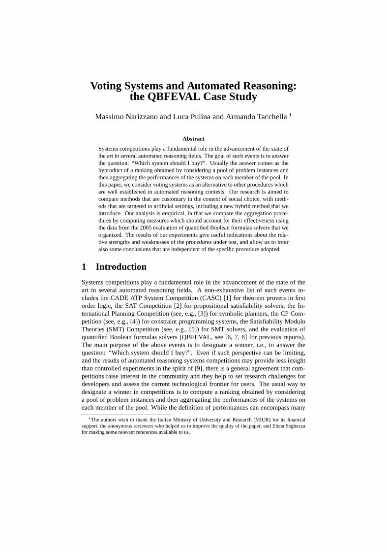
Method Mean Std Median Min Max IQ Range FQBF 182.25 7.53 183 170 192 13 88.54CASC 182.25 7.53 183 170 192 13 88.54SAT 87250 12520.2 83262.33 78532.74 119780.48 4263.94 65.56YASM 46.64 2.22 46.33 43.56 51.02 2.82 85.38YASMv2 1257.29 45.39 1268.73 1198.43 1312.72 95.11 91.29Borda 984.5 127.39 982.5 752 1176 194.5 63.95r. v. 12010.25 5183.86 12104 5186 21504 8096 24.12SCHULZE – – – – – – –

Table 2: Fidelity of aggregation procedures. As far asSAT is concerned, the seriespurse is not assigned.

rankings, but, at the same time,(ii) do not yield antithetic solver rankings. Thus, ho-mogeneity is not an effectiveness measure per se, but it is a preliminary assessment thatwe are performing an apple-to-apple comparison and that the apples are not exactly thesame.

Homogeneity is computed as in [17] considering the Kendall rank correlation co-efficientτ which is a nonparametric coefficient best suited to compare rankings.τ iscomputed between any two rankings and it is such that−1 ≤ τ ≤ 1, whereτ = −1means perfect disagreement,τ = 0 means independence, andτ = 1 means perfectagreement. Table 1 shows the values ofτ computed for the aggregation proceduresconsidered, arranged in a symmetric matrix where we omit the elements below thediagonal (r.v. is a shorthand for range voting). Values ofτ close to, but not exactlyequal to1 are desirable. Table 1 shows that this is indeed the case for the aggregationprocedures considered using QBFEVAL’05 data. Only two couples of methods (QBF-CASC and Schulze-Borda) show perfect agreement, while all the other couples agreeto some extent, but still produce different rankings.

4.2 Fidelity

We introduce this measure to check whether the aggregation procedures under testintroduce any distortion with respect to the true merits of the solvers. Our motiva-tion is that we would like to extract some scientific insight from the final ranking ofQBFEVAL’06 and not just winners and losers. Of course, we have no way to knowthe true merits of the QBF solvers: this would be like knowing the true statistic ofsome population. Therefore, we measure fidelity by feeding each aggregation proce-dure with “white noise”, i.e., several samples of table RUNS having the same structureoutlined in Subsection 2.1 and filled with random results. In particular, we assign toRESULT one ofSAT/UNSAT, TIME andFAIL values with equal probability, and a valueof CPUTIME chosen uniformly at random in the interval [0;1]. Given this artificial set-ting, we know in advance that the true merit of the competitors is approximately thesame. A high-fidelity aggregation procedure is thus one that computes approximatelythe same scores for each solver, and thus produces a final ranking where scores have asmall variance-to-mean ratio.

The results of the fidelity test are presented in Table 2 where each line contains thestatistics of a aggregation procedure. The columns show, from left to right, the mean,

Figure 1: RDT-stability plots.

the standard deviation, the median, the minimum, the maximum and the interquartilerange of the scores produced by each aggregation procedure when fed by white noise.The last column is our fidelity coefficient F, i.e., the percent ratio between the lowestscore (solver ranked last) and the highest one (solver ranked first): the higher the valueof F, the more the fidelity of the aggregation procedure. As we can see from Table 2,the fidelity of YASMv2 is better than that of all the other methods under test, includingQBF and CASC which are second best, and have higher fidelity than YASM. Noticethat range voting, and to a lesser extent also SAT and Borda’s methods, introduce asubstantial distortion. In the case of range voting, this can be explained by the ex-ponential spread that separates the scores, and thus amplifies even small differences.Measuring fidelity does not make sense in the case of Schulze’s method. Indeed, giventhe characteristics of the "white noise" data set, Schulze’s method yields a tie amongall the solvers. Thus, checking for fidelity would essentially mean checking the tie-breaking heuristic, and not the main method.

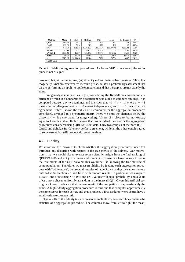
4.3 RDT-stability and DTL-stability

Stability on a randomized decreasing test set (RDT-stability), and stability on a de-creasing time limit (DTL-stability) have been introduced in [17] to measure how muchan aggregation procedure is sensitive to perturbations that diminish the size of the orig-inal test set, and how much an aggregation procedure is sensitive to perturbations thatdiminish the maximum amount of CPU time granted to the solvers, respectively. Theresults of RDT- and DTL-stability tests are presented in the plots of Figures 1 and 2.We obtained such plots considering the CPU time noise model in [18], and consideringYASMv2 instead of YASM and the Schulze’s method instead of the sum of victoriesmethod.On Figure 1, the first row shows, from left to right, the plots regarding QBF/CASC,SAT and YASMv2 procedures, while the second row shows, again from left to right,the plots regarding Borda’s method, range voting and Schulze’s method. Each his-togram reports, on the x-axis the number of problemsm discarded from the origi-

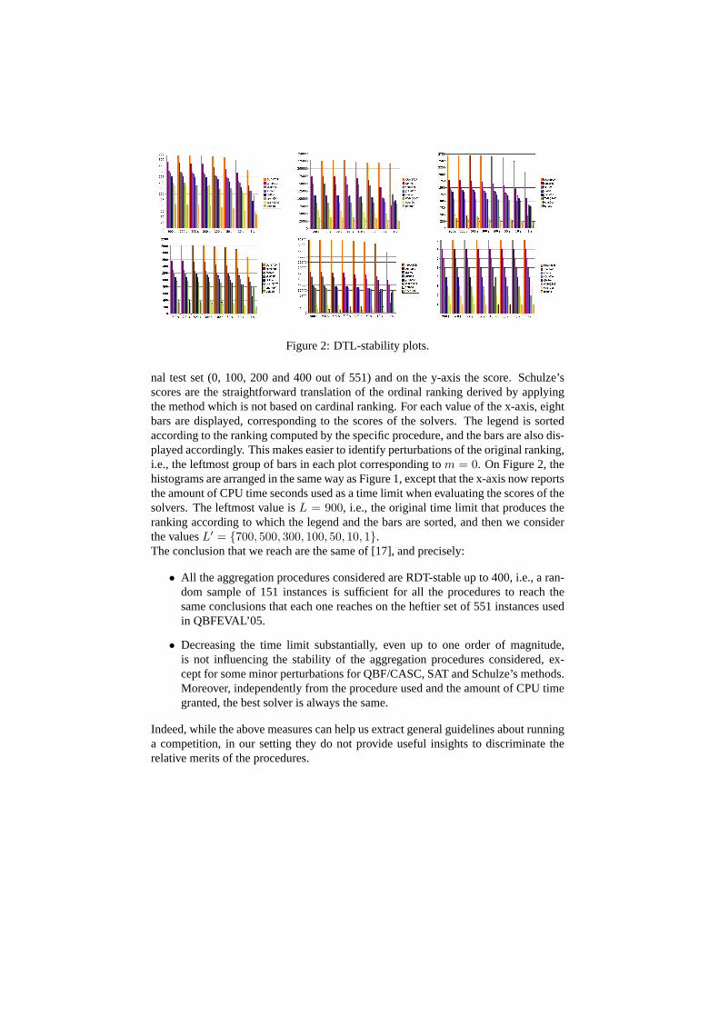
Figure 2: DTL-stability plots.

nal test set (0, 100, 200 and 400 out of 551) and on the y-axis the score. Schulze’sscores are the straightforward translation of the ordinal ranking derived by applyingthe method which is not based on cardinal ranking. For each value of the x-axis, eightbars are displayed, corresponding to the scores of the solvers. The legend is sortedaccording to the ranking computed by the specific procedure, and the bars are also dis-played accordingly. This makes easier to identify perturbations of the original ranking,i.e., the leftmost group of bars in each plot corresponding tom = 0. On Figure 2, thehistograms are arranged in the same way as Figure 1, except that the x-axis now reportsthe amount of CPU time seconds used as a time limit when evaluating the scores of thesolvers. The leftmost value isL = 900, i.e., the original time limit that produces theranking according to which the legend and the bars are sorted, and then we considerthe valuesL′ = {700, 500, 300, 100, 50, 10, 1}.The conclusion that we reach are the same of [17], and precisely:

• All the aggregation procedures considered are RDT-stable up to 400, i.e., a ran-dom sample of 151 instances is sufficient for all the procedures to reach thesame conclusions that each one reaches on the heftier set of 551 instances usedin QBFEVAL’05.

• Decreasing the time limit substantially, even up to one order of magnitude,is not influencing the stability of the aggregation procedures considered, ex-cept for some minor perturbations for QBF/CASC, SAT and Schulze’s methods.Moreover, independently from the procedure used and the amount of CPU timegranted, the best solver is always the same.

Indeed, while the above measures can help us extract general guidelines about runninga competition, in our setting they do not provide useful insights to discriminate therelative merits of the procedures.

Figure 3: SBT-stability plots.

4.4 SBT-stability

Stability on a solver biased test set (SBT-stability) is introduced in [17] to measure howmuch an aggregation procedure is sensitive to a test set that is biased in favor of a givensolver. LetΓ be the original test set, andΓs be the subset ofΓ such that the solvers isable to solve exactly the instances inΓs. LetRq,s be the ranking obtained by applyingthe aggregation procedureq onΓs. If Rq,s is the same as the original rankingRq, thenthe aggregation procedureq is SBT-stable with respect to the solvers. Notice that,contrarily to what stated in [17], SBT-stability alone is not a sufficient indicator of thecapacity of an aggregation procedure to detect the absolute merit of the participants.Indeed, it turns out that a very low-fidelity method such as range voting is remarkablySBT-stable. This because we can raise the SBT-stability of a ranking by decreasing itsfidelity: in the limit, a aggregation procedure that assigns fixed scores to each solver,has the best SBT-stability and the worst fidelity. Therefore, an aggregation procedureshowing a high SBT-stability is relatively immune to bias in the test set, but it mustalso feature a high fidelity if we are to conclude that the method provides a good hintat detecting the absolute merit of the solvers.

Figure 3 shows the plots with the results of the SBT-stability measure for eachaggregation procedure considering the noise model and YASMv2 (the layout is thesame as Figures 1 and 2). The x-axis reports the name of the solvers used to computethe solver-biased test setΓs and the y-axis reports the score value. For each of theΓs’s, we report eight bars showing the scores obtained by the solvers using only theinstances inΓs. The order of the bars (and of the legend) corresponds to the rankingobtained with the given aggregation procedure on the original test setΓ. As we can seefrom Figure 3 (top-left), CASC/QBF aggregation procedures are not SBT-stable: foreach of theΓs, the original ranking is perturbed and the winner becomess. Notice thaton ΓQUANTOR, CASC/QBF yield the same ranking that they output on the completetest setΓ. The SAT competition procedure (Figure 3, top-center) is not SBT-stable,not even on the test set biased on its alleged winnerQUANTOR. YASMv2 is betterthan both CASC/QBF and SAT, since its alleged winnerQUANTOR is the winner on

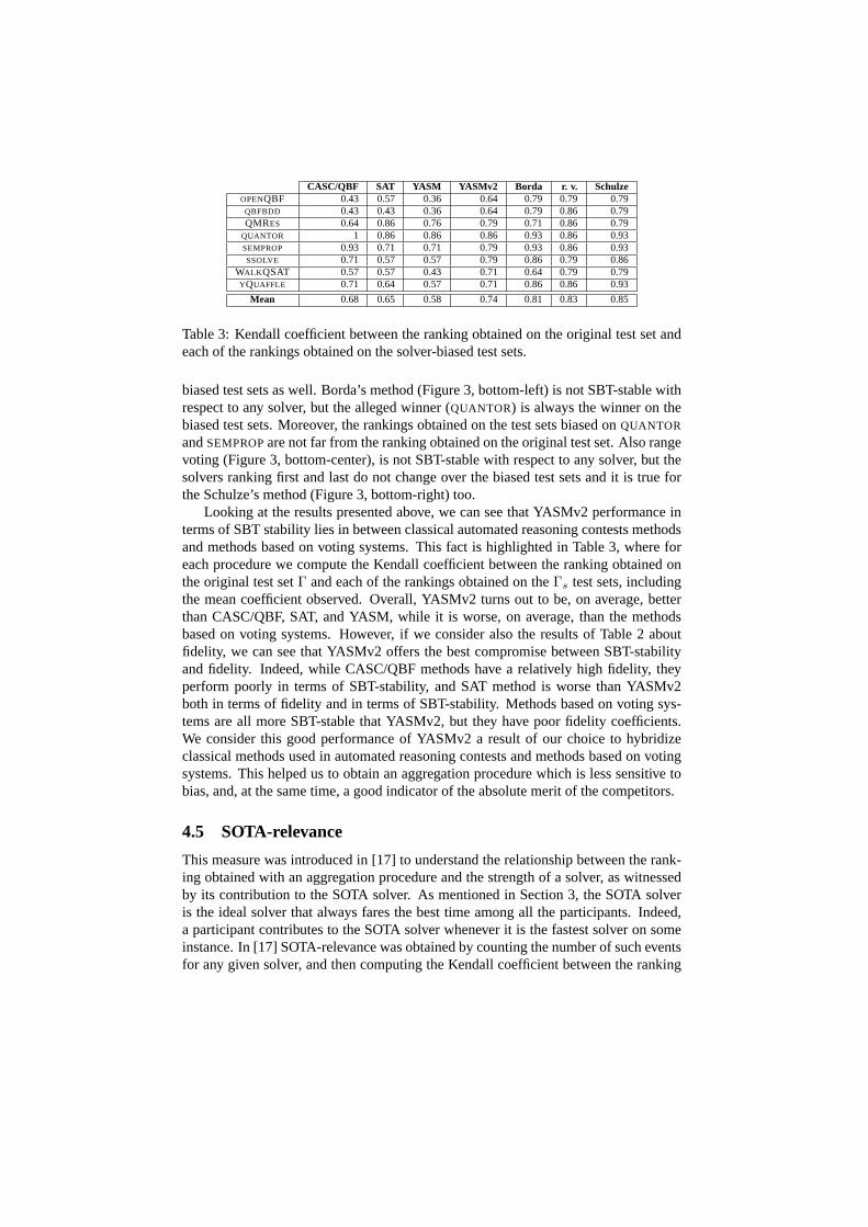
CASC/QBF SAT YASM YASMv2 Borda r. v. SchulzeOPENQBF 0.43 0.57 0.36 0.64 0.79 0.79 0.79QBFBDD 0.43 0.43 0.36 0.64 0.79 0.86 0.79QMRES 0.64 0.86 0.76 0.79 0.71 0.86 0.79

QUANTOR 1 0.86 0.86 0.86 0.93 0.86 0.93SEMPROP 0.93 0.71 0.71 0.79 0.93 0.86 0.93SSOLVE 0.71 0.57 0.57 0.79 0.86 0.79 0.86

WALK QSAT 0.57 0.57 0.43 0.71 0.64 0.79 0.79YQUAFFLE 0.71 0.64 0.57 0.71 0.86 0.86 0.93

Mean 0.68 0.65 0.58 0.74 0.81 0.83 0.85

Table 3: Kendall coefficient between the ranking obtained on the original test set andeach of the rankings obtained on the solver-biased test sets.

biased test sets as well. Borda’s method (Figure 3, bottom-left) is not SBT-stable withrespect to any solver, but the alleged winner (QUANTOR) is always the winner on thebiased test sets. Moreover, the rankings obtained on the test sets biased onQUANTOR

andSEMPROPare not far from the ranking obtained on the original test set. Also rangevoting (Figure 3, bottom-center), is not SBT-stable with respect to any solver, but thesolvers ranking first and last do not change over the biased test sets and it is true forthe Schulze’s method (Figure 3, bottom-right) too.

Looking at the results presented above, we can see that YASMv2 performance interms of SBT stability lies in between classical automated reasoning contests methodsand methods based on voting systems. This fact is highlighted in Table 3, where foreach procedure we compute the Kendall coefficient between the ranking obtained onthe original test setΓ and each of the rankings obtained on theΓs test sets, includingthe mean coefficient observed. Overall, YASMv2 turns out to be, on average, betterthan CASC/QBF, SAT, and YASM, while it is worse, on average, than the methodsbased on voting systems. However, if we consider also the results of Table 2 aboutfidelity, we can see that YASMv2 offers the best compromise between SBT-stabilityand fidelity. Indeed, while CASC/QBF methods have a relatively high fidelity, theyperform poorly in terms of SBT-stability, and SAT method is worse than YASMv2both in terms of fidelity and in terms of SBT-stability. Methods based on voting sys-tems are all more SBT-stable that YASMv2, but they have poor fidelity coefficients.We consider this good performance of YASMv2 a result of our choice to hybridizeclassical methods used in automated reasoning contests and methods based on votingsystems. This helped us to obtain an aggregation procedure which is less sensitive tobias, and, at the same time, a good indicator of the absolute merit of the competitors.

4.5 SOTA-relevance

This measure was introduced in [17] to understand the relationship between the rank-ing obtained with an aggregation procedure and the strength of a solver, as witnessedby its contribution to the SOTA solver. As mentioned in Section 3, the SOTA solveris the ideal solver that always fares the best time among all the participants. Indeed,a participant contributes to the SOTA solver whenever it is the fastest solver on someinstance. In [17] SOTA-relevance was obtained by counting the number of such eventsfor any given solver, and then computing the Kendall coefficient between the ranking

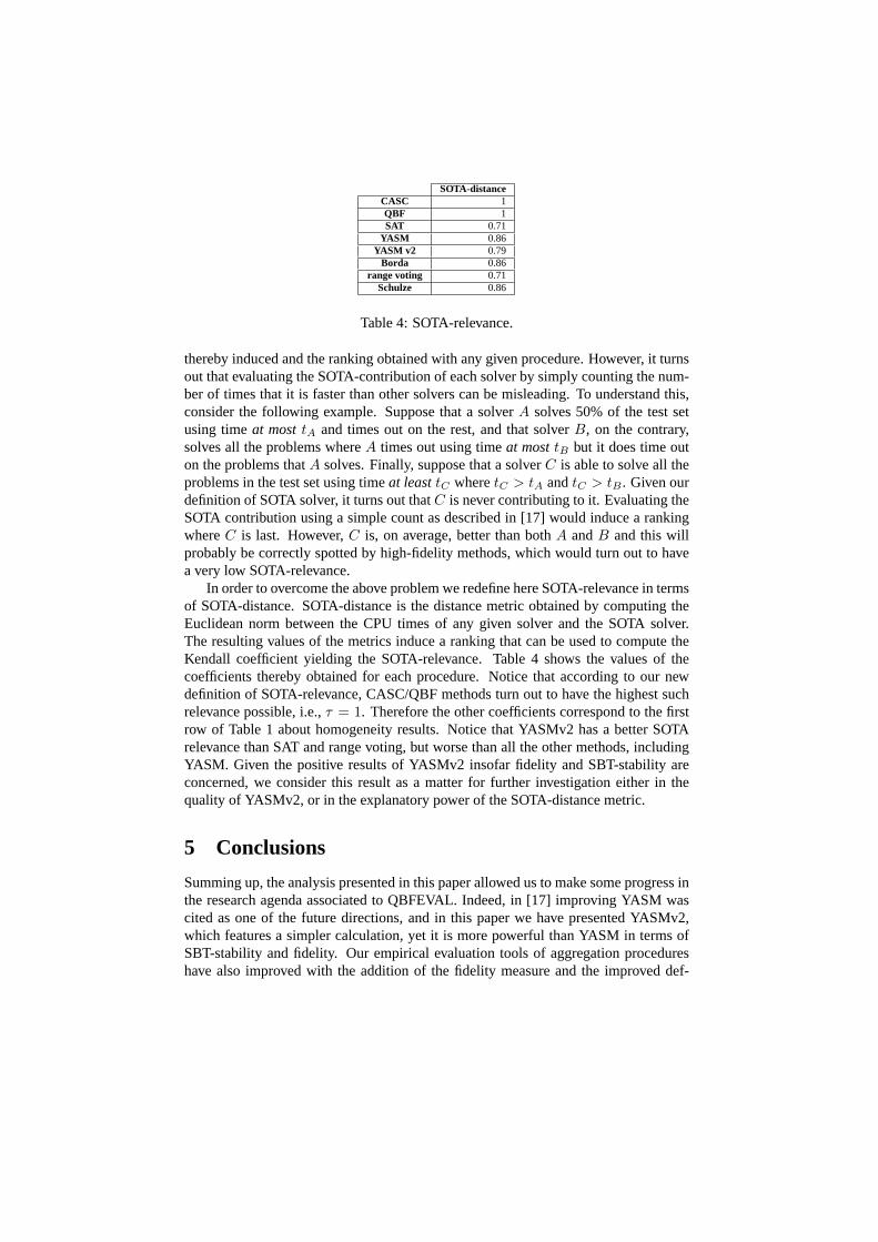
SOTA-distanceCASC 1QBF 1SAT 0.71

YASM 0.86YASM v2 0.79

Borda 0.86range voting 0.71

Schulze 0.86

Table 4: SOTA-relevance.

thereby induced and the ranking obtained with any given procedure. However, it turnsout that evaluating the SOTA-contribution of each solver by simply counting the num-ber of times that it is faster than other solvers can be misleading. To understand this,consider the following example. Suppose that a solverA solves 50% of the test setusing timeat mosttA and times out on the rest, and that solverB, on the contrary,solves all the problems whereA times out using timeat mosttB but it does time outon the problems thatA solves. Finally, suppose that a solverC is able to solve all theproblems in the test set using timeat leasttC wheretC > tA andtC > tB . Given ourdefinition of SOTA solver, it turns out thatC is never contributing to it. Evaluating theSOTA contribution using a simple count as described in [17] would induce a rankingwhereC is last. However,C is, on average, better than bothA andB and this willprobably be correctly spotted by high-fidelity methods, which would turn out to havea very low SOTA-relevance.

In order to overcome the above problem we redefine here SOTA-relevance in termsof SOTA-distance. SOTA-distance is the distance metric obtained by computing theEuclidean norm between the CPU times of any given solver and the SOTA solver.The resulting values of the metrics induce a ranking that can be used to compute theKendall coefficient yielding the SOTA-relevance. Table 4 shows the values of thecoefficients thereby obtained for each procedure. Notice that according to our newdefinition of SOTA-relevance, CASC/QBF methods turn out to have the highest suchrelevance possible, i.e.,τ = 1. Therefore the other coefficients correspond to the firstrow of Table 1 about homogeneity results. Notice that YASMv2 has a better SOTArelevance than SAT and range voting, but worse than all the other methods, includingYASM. Given the positive results of YASMv2 insofar fidelity and SBT-stability areconcerned, we consider this result as a matter for further investigation either in thequality of YASMv2, or in the explanatory power of the SOTA-distance metric.

5 Conclusions

Summing up, the analysis presented in this paper allowed us to make some progress inthe research agenda associated to QBFEVAL. Indeed, in [17] improving YASM wascited as one of the future directions, and in this paper we have presented YASMv2,which features a simpler calculation, yet it is more powerful than YASM in terms ofSBT-stability and fidelity. Our empirical evaluation tools of aggregation procedureshave also improved with the addition of the fidelity measure and the improved def-

inition of SOTA-relevance. We confirmed some of the conclusions reached in [17],namely that independently of the specific procedure used, a larger test set is not nec-essarily a better test set, and that a higher time limit does not necessarily result in amore informative contest. On the other hand, while aggregation procedures based onvoting systems emerged from [17] as “moral” winners over other procedures, the anal-ysis presented in this paper shows that better results could be achieved using hybridtechniques such as YASMv2.

References

[1] G. Sutcliffe and C. Suttner. The CADE ATP System Competition.http://www.cs.miami.edu/~tptp/CASC [2006-6-2].

[2] D. Le Berre and L. Simon. The SAT Competition. http://www.satcompetition.org [2006-6-2].

[3] D. Long and M. Fox. The 3rd International Planning Competition: Results andAnalysis.Artificial Intelligence Research, 20:1–59, 2003.

[4] M.R.C. van Dongen. Introduction to the Solver Competition. InCPAI 2005proceedings, 2005.

[5] C. W. Barrett, L. de Moura, and A. Stump. SMT-COMP: Satisfiability Mod-ulo Theories Competition. InCAV, volume 3576 ofLecture Notes in ComputerScience, pages 20–23, 2005.

[6] D. Le Berre, L. Simon, and A. Tacchella. Challenges in the QBF arena: theSAT’03 evaluation of QBF solvers. InSixth International Conference on Theoryand Applications of Satisfiability Testing (SAT 2003), volume 2919 ofLectureNotes in Computer Science. Springer Verlag, 2003.

[7] D. Le Berre, M. Narizzano, L. Simon, and A. Tacchella. The second QBF solversevaluation. InSeventh International Conference on Theory and Applications ofSatisfiability Testing (SAT 2004), Lecture Notes in Computer Science. SpringerVerlag, 2004.

[8] M. Narizzano, L. Pulina, and A. Tacchella. The third QBF solvers comparativeevaluation.Journal on Satisfiability, Boolean Modeling and Computation, 2:145–164, 2006. Available on-line athttp://jsat.ewi.tudelft.nl/ .

[9] J. N. Hooker. Testing Heuristics: We Have It All Wrong.Journal of Heuristics,1:33–42, 1996.

[10] D. G. Saari. Chaotic Elections! A Mathematician Looks at Voting. AmericanMathematical Society, 2001.

[11] W. D. Smith. Range voting. Available on-line athttp://www.math.temple.edu/~wds/homepage/rangevote.pdf [2006-9-29].

[12] M. Schulze. A New Monotonic and Clone-Independent Single-Winner ElectionMethod.Voting Matters, pages 9–19, 2003.

[13] M. Narizzano, L. Pulina, and A. Taccchella. QBF solvers competitive evaluation(QBFEVAL). http://www.qbflib.org/qbfeval .

[14] RoboCup.http://www.robocup.org .

[15] K. J. Arrow, A. K. Sen, and K. Suzumura, editors.Handbook of Social Choiceand Welfare, volume 1. Elsevier, 2002.

[16] V. Conitzer and T. Sandholm. Common Voting Rules as Maximum LikelihoodEstimators. In6th ACM Conference on Electronic Commerce (EC-05), LectureNotes in Computer Science, pages 78–87, 2005.

[17] L. Pulina. Empirical Evaluation of Scoring Methods. InProc. STAIRS 2006,volume 142 ofFrontiers in Artificial Intelligence and Applications, pages 108–119, 2006.

[18] M. Narizzano, L. Pulina, and A. Tacchella. Competitive Evaluation of QBFSolvers: noisy data and scoring methods. Technical report, STAR-Lab - Uni-versity of Genoa, May 2006.

[19] E. Giunchiglia, M. Narizzano, and A. Tacchella. Quantified Boolean Formulassatisfiability library (QBFLIB), 2001.www.qbflib.org .

[20] A. Van Gelder, D. Le Berre, A. Biere, O. Kullmann, and L. Simon. Purse-BasedScoring for Comparison of Exponential-Time Programs, 2006. Unpublisheddraft.

[21] M. Narizzano, L. Pulina, and A. Tacchella. Competitive Evaluation of AutomatedReasoning Tools: Statistical Testing and Empirical Scoring. InFirst Workshopon Empirical Methods for the Analysis of Algorithms (EMAA 2006), 2006.

[22] M. Schulze. Extending schulze’s method to obtain an overall ranking. Personalcommunications.

Massimo NarizzanoDIST, Università di GenovaViale Causa, 13 – 16145 Genova, ItalyEmail:mox@dist.unige.it

Luca PulinaDIST, Università di GenovaViale Causa, 13 – 16145 Genova, ItalyEmail:pulina@dist.unige.it

Armando TacchellaDIST, Università di GenovaViale Causa, 13 – 16145 Genova, ItalyEmail: tac@dist.unige.it