Visual voice activity detection as a help for speech

source separation from convolutive mixtures

Bertrand Rivet, Laurent Girin, Christian Jutten

To cite this version:

Bertrand Rivet, Laurent Girin, Christian Jutten. Visual voice activity detection as a help forspeech source separation from convolutive mixtures. Speech Communication, Elsevier, 2007,49 (7-8), pp.667-677. <10.1016/j.specom.2007.04.008>. <hal-00174131>

HAL Id: hal-00174131

https://hal.archives-ouvertes.fr/hal-00174131

Submitted on 21 Sep 2007

HAL is a multi-disciplinary open accessarchive for the deposit and dissemination of sci-entific research documents, whether they are pub-lished or not. The documents may come fromteaching and research institutions in France orabroad, or from public or private research centers.

L’archive ouverte pluridisciplinaire HAL, estdestinee au depot et a la diffusion de documentsscientifiques de niveau recherche, publies ou non,emanant des etablissements d’enseignement et derecherche francais ou etrangers, des laboratoirespublics ou prives.

Visual voice activity detection as an help

for speech source separation

from convolutive mixtures

Bertrand Rivet a,b,∗ Laurent Girin a Christian Jutten b

aInstitut de la Communication Parlee (ICP)(CNRS UMR 5009, INPG, Universite Stendhal), Grenoble, France

bLaboratoire des Images et des Signaux (LIS)(CNRS UMR 5083, INPG, Universite Joseph Fourier), Grenoble, France

Abstract

Audio-visual speech source separation consists in mixing visual speech processingtechniques (e.g., lip parameters tracking) with source separation methods to improvethe extraction of a speech source of interest from a mixture of acoustic signals. Inthis paper, we present a new approach that combines visual information with sep-aration methods based on the sparseness of speech: visual information is used asa voice activity detector (VAD) which is combined with a new geometric methodof separation. The proposed audiovisual method is shown to be efficient to extracta real spontaneous speech in the difficult case of convolutive mixtures even if thecompeting sources are highly non-stationary. Typical gains of 18-20dB in signal tointerference ratios are obtained for a wide range of (2×2) and (3×3) mixtures. More-over, the overall process is quite computationally simpler than previously proposedaudiovisual separation schemes.

Key words: speech source separation, convolutive mixtures, voice activitydetector, speech enhancement, highly non-stationary environments.

1 Introduction

Audio-visual speech source separation (AVSSS) is a growing field of interestto solve the source separation problem when speech signals are involved. Itconsists in exploiting the bimodal (audio-visual) nature of speech to improve

∗ Corresponding author: rivet@icp.inpg.fr

Preprint submitted to Elsevier Science 31 January 2006

the performance or supply the weaknesses of acoustic speech signals separa-tion [1,2]. For instance, pioneer works by Girin et al. [3] and then Sodoyeret al. [4] have proposed to use a statistical model of the coherence of au-dio and visual speech features to estimate the separating matrix for additivemixtures. Later, Dansereau [5] and Rajaram et al. [6] respectively pluggedthe visual information in a 2 × 2 decorrelation system with first-order filtersand in the Bayesian framework for a 2 × 2 linear mixture. Unfortunately,real audio mixtures are generally intricate and better described as convolutivemixtures with quite long filters. Recently, Rivet et al. [7] have proposed a firstapproach to exploit visual speech information in such convolutive mixtures.Visual parameters were used to regularize the permutation and the scale factorindeterminacies that arise at each frequency bin in frequency-domain separa-tion methods [8–11]. In parallel, the audiovisual (AV) coherence maximizationapproach was also considered for the estimation of deconvolution filters in [12].

In this paper, we propose a simpler and efficient approach for the same prob-lem (extracting one speech source from convolutive mixtures). First we pro-pose to use visual speech information, for instance lip movements, as a voiceactivity detector (VAD): the task is to assess the presence or the absence ofa given speaker’s speech signal in the mixture, a crucial information to befurther used in separation processes. Such visual VAD (V-VAD) is character-ized by a major advantage as opposed to usual acoustic VADs: it is robust toany acoustic environment, whatever the nature and the number of competingsources (e.g. simultaneous speaker(s), non-stationary noises, convolutive mix-ture, etc.). Note that previous work on VAD based on visual information canbe found in [13]. The authors proposed to model the distribution of the visualinformation using two exclusive classes (one for speech non-activity and onefor actual speech activity): the decision is then based on likelihood criterion.However, the presented approach is completely different since we exploit thetemporal dynamic of lip movements and we do not use an a priori statisticalmodel (Section 2).

Secondly, we propose a geometric approach of the extraction process exploitingthe sparseness of the speech signals (Section 3). One of the major drawback ofthe frequency-domain separation methods is the need for regularizing the in-determinacies encountered at each frequency bin [14]. Indeed, the separation isgenerally done separately at each frequency bin by statistical considerations,and arbitrary permutations between estimated sources and arbitrary scalefactors can occur leading to a wrong reconstruction of the estimated sources.Several solutions to the permutation problem were proposed e.g. exploitingthe correlation over frequencies of the reconstructed sources [9,10], exploitingthe smoothness of the separating filters [11] or exploiting AV coherence [7].Alternately, other methods try to exploit the sparseness of the sources. Forinstance, Abrard and Deville in [15] proposed a solution in the case of instan-taneous mixture. They exploit the frequency sparseness of the sources: in the

2

time-frequency plane, areas where only one source is present are selected byusing an acoustic VAD, allowing the determination of the separating matrix.However, their method has two restrictions: i) it concerns instantaneous mix-tures while real mixtures are often convolutive, ii) it requires time-frequencyareas where only one source is present, which is a very strong assumption (thenumber of such areas is very small 1 ). Recently, Babaie-Zadeh et al. [16] pro-posed a geometric approach in the case of instantaneous mixtures of sparsesources. The method is based on the identification of the main direction ofthe present sources in the mixtures. Our proposed method is also geometricbut is quite different from their, since in our approach i) only the source to beextracted has to be sparse, ii) the indexation of the sections where the sourceto be extracted is absent is done thanks to the proposed V-VAD, iii) the caseof convolutive mixtures is addressed. Also, in addition to intrinsically solvethe permutation problem for the reconstructed source, the proposed methodis refined by an additional stage to regularize the scale factor ambiguity.

This paper is organized as follows. Section 2 presents the basis of the proposedV-VAD. Section 3 explains the proposed geometrical separation using theV-VAD first in the case of instantaneous mixtures and then in the case ofconvolutive mixtures. Section 4 presents both the analysis of the V-VAD andthe results of the AV separation process before conclusions in Section 5.

2 Visual voice activity detection

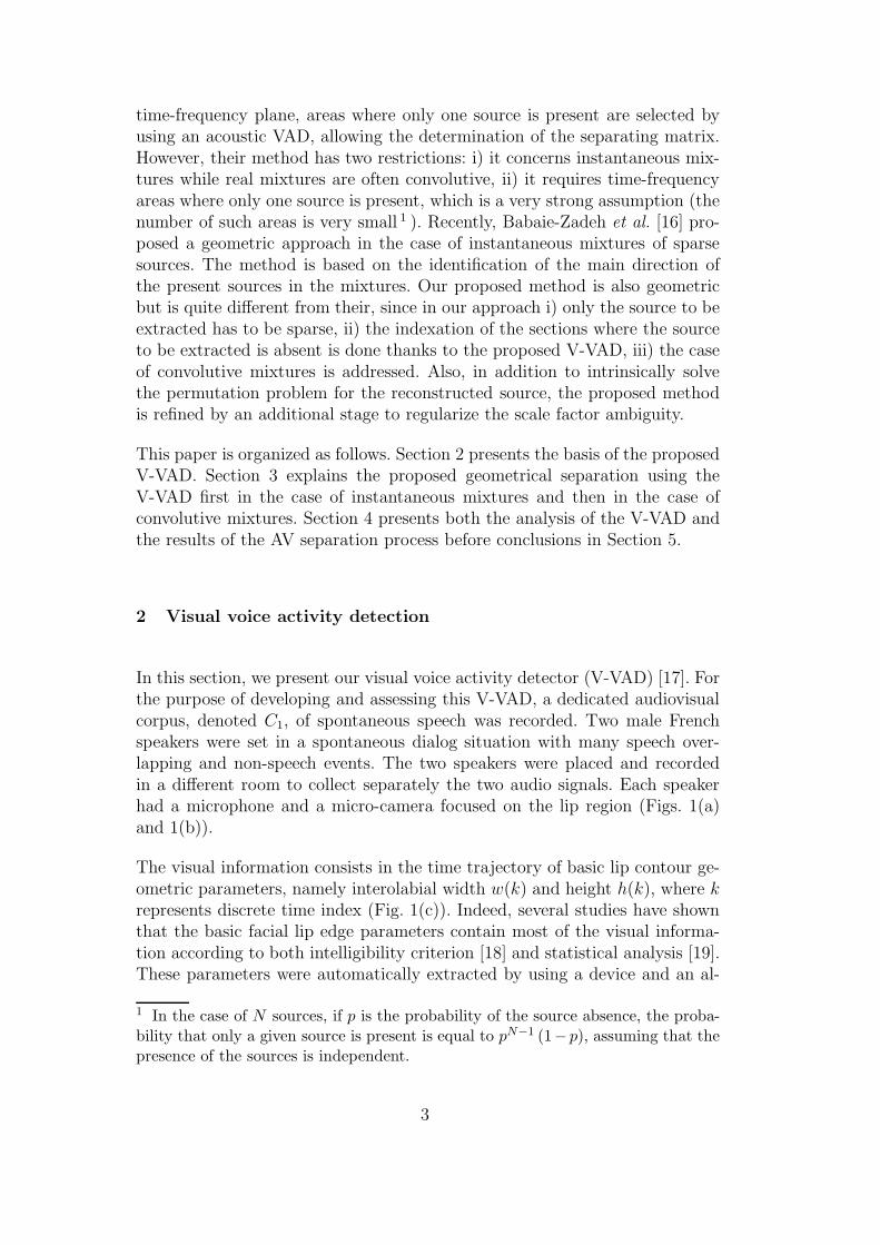
In this section, we present our visual voice activity detector (V-VAD) [17]. Forthe purpose of developing and assessing this V-VAD, a dedicated audiovisualcorpus, denoted C1, of spontaneous speech was recorded. Two male Frenchspeakers were set in a spontaneous dialog situation with many speech over-lapping and non-speech events. The two speakers were placed and recordedin a different room to collect separately the two audio signals. Each speakerhad a microphone and a micro-camera focused on the lip region (Figs. 1(a)and 1(b)).

The visual information consists in the time trajectory of basic lip contour ge-ometric parameters, namely interolabial width w(k) and height h(k), where krepresents discrete time index (Fig. 1(c)). Indeed, several studies have shownthat the basic facial lip edge parameters contain most of the visual informa-tion according to both intelligibility criterion [18] and statistical analysis [19].These parameters were automatically extracted by using a device and an al-

1 In the case of N sources, if p is the probability of the source absence, the proba-bility that only a given source is present is equal to pN−1 (1− p), assuming that thepresence of the sources is independent.

3

(a)

(b)

(c)

Fig. 1. Experimental conditions used to record the corpus C1 (Fig 1(a) and 1(b)).Fig. 1(c) presents the video parameters: internal width w and internal height h.

gorithm developed at the ICP [20]. The technique is based on blue make-up,Chroma-Key system and contour tracking algorithms. The parameters are ex-tracted every 20ms (the video sampling frequency is 50Hz), synchronouslywith the acoustic signal which is sampled at 16kHz. Thus in the following, anaudiovisual signal frame is a 20ms section of acoustic signal associated with avideo pair parameters (w(k), h(k)).

The aim of a voice activity detector (VAD) is to discriminate speech and non-speech sections of the acoustic signal. However, we prefer to use the distinctionbetween silence (defined as vocal inactivity) and non-silence sections for agiven speaker because non-speech sections are not bound to be silence, sincemany kinds of non-speech sounds can be produced by the speaker (e.g. laughs,sighs, growls, moans, etc.). Moreover, the separation system of Section 3 isbased on the detection of complete non activity of the speaker to be extractedfrom the mixture (i.e. no sound is produced by this speaker). To provide anobjective reference for the detection, we first manually identified and labeled

4

0 0.5 1 1.50

0.5

1

1.5

2

2.5

3

π1(k)

π2(k

)

(a)

0 0.5 1 1.50

0.5

1

1.5

2

2.5

3

π1(k)

π2(k

)

(b)

Fig. 2. Distribution of the visual parameter π(t) for non-silence frames (2(a)) andsilence frames (2(b)). Note that 10% and 36% of the points are at the origin (closedlip shape) for the 2(a) and 2(b) figures respectively.

acoustic sections of silence and non-silence. Then, we defined a normalizedvideo vector as π(k) = [w(k)/µw, α h(k)/µh]

T where α is the coefficient oflinear regression between w(k) and h(k), µw and µh the mean values of w(k)and h(k) calculated on the complete corpus for each speaker (T denotes thetranspose operator).

As explained in [17], a direct VAD from raw lip parameters cannot lead tosatisfactory performances because of the intricate relationship between visualand acoustic speech information. Indeed, Fig. 2 represents the distribution ofthe components π1(k) and π2(k) of π(k) for non-silence frames (Fig. 2(a)) andsilence frames (Fig.2(b)). One can see that there is no trivial partition be-tween the two classes (silence vs. non-silence): for instance, closed lip-shapesare present in both distributions and they cannot be systematically associatedwith a silence frame. The V-VAD [17] is based on the fact that silence framescan be better characterized by the lip-shape movements. Indeed, in silence sec-tions, the lip-shape variations are generally small, whereas in speech sectionsthese variations are generally quite stronger. So we proposed the followingdynamical video parameter

v(k) =

∣

∣

∣

∣

∣

∂π1(k)

∂k

∣

∣

∣

∣

∣

+

∣

∣

∣

∣

∣

∂π2(k)

∂k

∣

∣

∣

∣

∣

. (1)

The kth input frame is classified as silence if v(k) is lower than a thresholdand it is classified as speech otherwise. However, direct thresholding of v(k)do not provide optimal performances: for instance, the speaker’s lips may notmove during several frames, while he is actually speaking. Thus, we smooth

5

−4 −3 −2 −1 00

200

400

600

800

1000

(a)

−4 −3 −2 −1 00

200

400

600

800

1000

(b)

−4 −3 −2 −1 00

200

400

600

800

1000

(c)

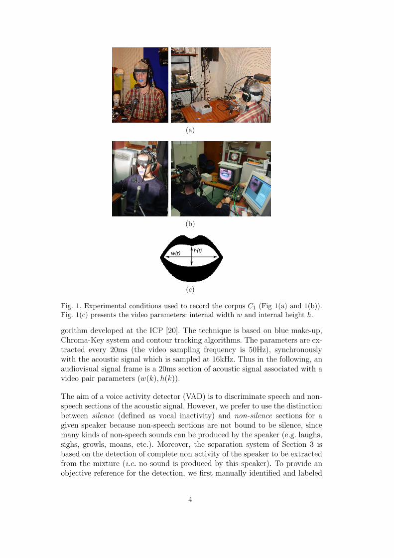
Fig. 3. Histograms of the dynamical visual parameter V (k) (on log-scale) for threeintegration durations: instantaneous (a), suitable value of α = .82 frames (b) andtoo large value of α = .99 (c). The black and white histograms respectively representthe V (k) values associated to silence and non-silence sections respectively.

v(k) by time integration over T consecutive frames

V (k) =T−1∑

l=0

αl v(k − l) (2)

where αl = αl are the coefficients of a truncated first-order IIR low-passfilter. Finally, the kth frame is classified as silence if V (k) is lower than athreshold δ (V (k) < δ) and speech otherwise (V (k) ≥ δ). Fig. 3 shows thatthe choice of the integration parameter α must be considered carefully. Atoo short α (or no integration) leads to a detection which is very sensitiveto local perturbations (Fig. 3(a)). On the contrary, a too large α leads toa quite incorrect detection (Fig. 3(c)). Fig. 3(b) shows that the choice of αcan largely improve the separation of silence and non-silence sections. Sincethe aim of the V-VAD, as explained in Section 3, is to detect frames wherethe speaker does not produce sounds, we propose an additional stage beforethe decision in order to decrease the false alarm (silence decision while speechactivity). Only sequences of at least L frames of silence are actually consideredas silences. Finally, the proposed V-VAD is robust to any acoustic noise andcan be exploited even in hardly non-stationary environment. The performanceof the proposed V-VAD is given in Subsection 4.1.

3 Speech source separation using visual voice activity detector

In this section, we present the new geometrical method to extract one source ofinterest, say s1(k), from the observations x(k). The main idea of the proposedmethod is to exploit both i) the “sparseness” specificity of speech signals:in real spontaneous speech situations (e.g. dialog), there exist some periods(denoted “silence”) during which each speaker is silent as said in Section 2, ii)the possibility to detect these silent sections by using the V-VAD of Section 2.Note that the method allows the source with detected silence sections to be

6

extracted from the mixtures. If other sources are to be extracted, they shouldhave their own associated silence detector. We first explain the principle of theseparation process in the simple case of complex instantaneous mixtures, thenwe extend it to convolutive mixtures. We use the complex value for purpose ofgenerality because in the case of convolutive mixture, complex spectral valueswill be considered.

3.1 Case of complex instantaneous mixtures

Let consider the case of N complex independent centered sources s(k) ∈ CN

and N complex observations x(k) ∈ CN obtained by a complex mixing matrixA ∈ C

N×N :

x(k) = A s(k) (3)

where s(k) = [s1(k), · · · , sN(k)]T and x(k) = [x1(k), · · · , xN(k)]T . We supposethat A is invertible. Thus to extract the sources s(k), we have to estimate aseparating matrix B ∈ CN×N , which is typically an estimate of the inverseof A. It is a classical property of usual source separation systems that theseparation can only be done up to a permutation and a scaling factor [14],that is

B ≃ P DA−1 (4)

where P is a permutation matrix and D is a diagonal matrix. Let denoteC = BA the global matrix. Thus, to extract the first source s1(k), only onerow of B is necessary, we arbitrary choose the first one, denoted b1,·

2 :

s1(k) = b1,· x(k) = b1,·A s(k) ≃ c1,1 s1(k). (5)

In the following, we propose a novel method to estimate b1,·. Moreover, wego one step further by regularizing the scale factor so that the source s1(k) isestimated up to a1,1 instead of c1,1. This corresponds to the situation wherethe estimation of the source s1(k) is equal to the signal of x1(k) when the othersources vanish (in other words, s1(k) is estimated up to its channel+sensorcoefficient a1,1 for the considered mixture).

To estimate b1,·, we propose a novel geometric method. The dimension ofthe spaces Ss and Sx, spanned by the sources s(k) and the observations x(k)

2 In this paper, bi,· = [bi,1, · · · , bi,N ], and b·,i = [b1,i, · · · , bN,i]T , where bi,j is the

(i, j)th element of matrix B.

7

respectively, is N (Fig. 4(a) and Fig. 4(b)). The space spanned by the con-tribution of source s1 in Sx is a straight line denoted D1 (Fig. 4(c)). Now,suppose that an oracle 3 gives us T , a set of time indexes when s1(k) vanishes,then the space S ′

x (resp. S ′s), spanned by x(k) (resp. s(k)), with k ∈ T is a

hyper-plane (i.e. space of dimension N − 1) of Sx (resp. Ss). Moreover, D1 isa supplementary space of S ′

x in Sx:

Sx = S ′x ⊕D1. (6)

Note that S ′x and D1 are not necessary orthogonal. Moreover, S ′

x is the spacespanned by the contribution of sources {s2(k), · · · , sN(k)} in Sx. Thus to ex-tract s1, we have to project the observations x(k) on a supplementary spaceof S ′

x (not necessary D1).

To find this supplementary space, a proposed solution is to use a principalcomponent analysis (PCA). Indeed, performing an eigenvalue decompositionof the covariance matrix C

xx= E{x(k)xH(k)} (.H denotes the complex con-

jugate transpose) of the observations x(k) with k ∈ T (the set of time indexeswhen s1(k) vanishes) provides N orthogonal (since C

xxis Hermitian) eigen-

vectors associated with N eigenvalues that represent the respective averagepowers of the N sources during time slots T . Since s1(k) is absent for k ∈ T ,the smallest eigenvalue within the eigenvalues set is to be associated to thissource (this smallest eigenvalue should be close to zero). The straight lineD′

1, spanned by the (row) eigenvector, denoted g = [1, g2, · · · , gN ] (g1 is arbi-trary chosen equal to 1), associated with the smallest eigenvalue, defines theorthogonal supplementary space of S ′

x in Sx:

Sx = S ′x

⊥⊕ D′

1. (7)

Thus, for all time indexes k (now including when source s1 is active), sources1(k) can be extracted thanks to (b1,· = g):

s1(k) = g x(k) ≃ c1,1s1(k) (8)

where c1,1 = a1,1 + b1,2 a2,1 + · · · + b1,N aN,1. Note that scaling factor c1,1 canbe interpreted as an uncheck distortion since D1 is, a priori, a supplementaryspace of S ′

x and not necessary the orthogonal supplementary space of S ′x. As

explained below (Subsection 3.2), in the convolutive case this distortion candramatically alter the estimation of the source.

Now, we address the last issue of fixing the scaling factor to a1,1 instead of c1,1,

i.e. we have to find a complex scalar λ such that s†1(k) = λ s1(k) ≃ a1,1 s1(k).

3 Such an oracle is provided by the V-VAD of Section 2.

8

Ssց

(a)

Sxց

(b)

Sxց

S ′x

↓D1↓

(c)

Sxց

S ′x

↓D′

1↓

(d)

Fig. 4. Illustration of the geometric method in the case of 3 observations obtainedby an instantaneous mixture of 3 uniform sources. Fig. 4(a) shows 3 independentsources (s1, s2, s3) (dots) with uniform distribution and Ss the space spanned bythem. Fig. 4(b) shows a 3 × 3 instantaneous mixture (x1, x2, x3) (dots) of thesesources and Sx the space spanned by the mixture. Fig. 4(c) shows S ′

x and D1 (solidline). Fig. 4(d) shows S ′

x and D′1 (solid line)

Thus λ is given by

λ =a1,1

a1,1 +∑

i>1 b1,i ai,1=

1

1 +∑

i>1 b1,i ai,1/a1,1(9)

where ∀ i, b1,i are known and the set {ai,1/a1,1}i has to be estimated. To es-timate these coefficients, we propose a procedure based on the cancellationof the contribution of s1(k) in the different mixtures xi(k). Thus, let denote

ǫi(βi) = E{

|xi(k) − βi s1(k)|2}

, where E{·} denote the expectation operator.

Since the sources are independent, we have thanks to (3) and (8)

ǫi(βi) = E{

|(ai,1 − βi c1,1)s1(k)|2}

+∑

j>1

E{

|ai,j sj(k)|2}

. (10)

9

Moreover, ∀ βi, ǫi(βi) is lower bounded by∑

j>1 E{

|ai,j sj(k)|2}

and the lower

bound is obtained for βi = ai,1/c1,1. Let denote βi the optimal estimation of

βi in the minimum mean square error sense. βi is classically given by:

βi = arg minβi

ǫi(βi) =E{x∗

i (k) s1(k)}

E{|s1(k)|2}(11)

where ·∗ denotes the complex conjugate. In practice, the expectation is re-placed by time averaging and βi is given by

βi =

∑Kk=1 x∗

i (k)s1(k)∑K

k=1 |s1(k)|2. (12)

So, λ is given by (9) where ai,1/a1,1 is replaced by βi/β1. Note that we use theratio ai,1/a1,1 rather than ai,1 alone since βi is equal to ai,1 up to the unknowncoefficient c1,1. Finally, the source s1(k) is estimated by

s†1(k) = λb1,· x(k) ≃ a1,1 s1(k). (13)

3.2 Case of convolutive mixtures

Let us now consider the case of convolutive mixtures of N centered sourcess(k) = [s1(k), · · · , sN(k)]T to be separated from N observations x(k) = [x1(k), · · · , xN (k)]T :

xm(k) =N

∑

n=1

hm,n(k) ∗ sn(k). (14)

The filters hm,n(k), which model the impulse response between the nth sourceand the mth sensor, are the entries of the global mixing filter matrix H(k).

The aim of the source separation is to recover the sources by using a dualfiltering process:

s†n(k) =N

∑

m=1

gn,m(k) ∗ xm(k) (15)

where gn,m(k) are the entries of the global separating filter matrix G(k) thatmust be estimated. The problem is generally considered in the frequency do-main [8–11] where the single convolutive problem becomes a set of F (thenumber of frequency bins) simple linear instantaneous problems with complexentries. For all frequency bins f

10

Xm(k, f)=N

∑

n=1

Hm,n(f)Sn(k, f) (16)

S†n(k, f)=

N∑

m=1

Gn,m(f)Xm(k, f) (17)

where Sn(k, f), Xm(k, f) and S†n(k, f) are the Short-Term Fourier Trans-

forms (STFT) of sn(k), xp(k) and s†n(k) respectively. Hm,n(f) and Gn,m(f)are the frequency responses of the mixing H(f) and demixing G(f) filters re-spectively. Since the mixing process is assumed to be stationary, H(f) andG(f) are not time-dependent, although the signals (i.e. sources, observations)may be non-stationary. In the frequency domain, the goal of the source sepa-ration is to estimate, at each frequency bin f , the separating filter G(f). Thiscan be done thanks to the geometric method proposed in section 3.1. Indeed,at each frequency bin f , (16) and (17) can be seen as a case of an instantaneouscomplex mixture problem. Thus, b1,·(f) is the eigenvector associated with thesmallest eigenvalue of the covariance matrix C

xx(f) = E{X(k, f)XH(k, f)}

with k ∈ T . Then, βi(f) is a function of frequency f and is estimated thanksto

βi(f) =

∑Kk=1 X∗

i (k, f)S1(k, f)∑K

k=1

∣

∣

∣S1(k, f)∣

∣

∣

2 . (18)

So λ(f) is given by

λ(f) =1

1 +∑

i>1 b1,i(f) ai,1(f)/a1,1(f)(19)

where ai,1(f)/a1,1(f) is replaced by βi(f)/β1(f). Finally, the source S1(k, f)is estimated by

S†1(k, f) = G1,·(f)X(k, f) ≃ H1,1(f) S1(k, f) (20)

where G1,·(f) = λ(f)b1,·(f). Note that in the convolutive case, if the scalefactor regularization λ(f) is not ensured, the source s1(k) is estimated up toan unknown filter which can perceptually alter the estimation of the source.On the contrary, performing the scale factor regularization ensures that thefirst source is estimated up to the filter h1,1(k) which corresponds to the “chan-nel+sensor” filter of the first observation. The complete method is summarizedin the following Algorithm 1.

11

Algorithm 1 Geometric separation in the convolutive case

Estimate index silence frames T using V-VAD (Section 2)Perform STFT on the audio observations xm(k) to obtain Xm(k, f)for all frequency bins f do

{Estimation of b1,·(f)}Compute C

xx(f) = E{X(k, f)XH(k, f)} with k ∈ T

Perform eigenvalue decomposition of Cxx

(f)Select g(f) the eigenvector associated with the smallest eigenvalueb1,·(f) ⇐ g(f)

{Estimation of λ(f) to fix the scaling factor}Estimate βi(f) with (18)λ(f) is given by (19) where ai,1(f)/a1,1(f) is replaced by βi(f)/β1(f)

{Estimation of the demixing filter}G1,·(f) ⇐ λ(f)b1,·(f)

end for

Perform inverse Fourier transform of G1,·(f) to obtain G1,·(k)Estimate source s1(k) thanks to (15)

4 Numerical experiments

In this section, we first present the results about the V-VAD and next theresults of the geometric separation. All these experiments were performedusing real speech/acoustic signals. The audiovisual corpus denoted C1 usedfor the source to be extracted, say s1(k), consists of spontaneous male speechrecorded in dialog condition (Section 2). Two others corpus, denoted C2 andC3 respectively, consist of phonetically well-balanced sentences in French of adifferent male speaker and of acoustic noise recorded in a train, respectively.

4.1 Visual voice activity detector results

We tested the proposed V-VAD on about 13200 20ms-frames of corpus C1,representing about 4.4min of spontaneous speech. First of all, Fig. 5 illustratesthe different possible relations between visual and acoustic data: i) movementof the lips in non-silence (e.g. for time index k ∈ [3s, 4s]), ii) movement of thelips in silence (e.g. for time index k ∈ [2s, 2.3s]), iii) non-movement of the lipsin silence (e.g. for time index k ∈ [1.5s, 2s]), iv) non-movement of the lips innon-silence (e.g. for time index k ∈ [.9s, 1.1s]).

The detection results of the proposed V-VAD are presented as Receiver Op-erating Characteristics (ROC) (Fig. 6). These curves present the percentageof silence detection (i.e. ratio between the number of actual silence framesdetected as silence frames and the number of actual silence frames) versus

12

0 0.5 1 1.5 2 2.5 3 3.5−0.3

−0.2

−0.1

0

0.1

0 0.5 1 1.5 2 2.5 3 3.50

1

2

0 0.5 1 1.5 2 2.5 3 3.5−3

−2

−1

0

time [s]

Fig. 5. Silence detection. Top: acoustic speech signal with silence reference (solidline), frames detected as silence (dotted line) and frames eventually retained assilence when L = 20 consecutive silence frames (dashed line). Middle: static visualparameters π1(k) (solid line) and π2(k) (dashed line). Bottom: logarithm of thedynamical visual parameter V (k) integrated with αt = 0.82t (solid line, truncatedat -3) and the logarithm of the threshold δ (dashed line).

the percentage of false silence detection (i.e. ratio between the number of ac-tual non-silence frames detected as silence frames and the number of actualsilence frames). Fig.6(a) highlights the importance of the time integration bya low-pass filter of the video parameter v(k) (1). Indeed, by lessening the in-fluence of short movement of the lips in silence and the influence of the shortstatic lips in speech, the time integration (2) allows to improve the perfor-mance of the V-VAD: the false silence detection significantly decreases for agiven silence detection percentage (e.g. for 80% of correct silence detection, thefalse silence detection decreases from 20% to 5% with a correct integration).Furthermore, Fig. 6(b) shows the effect of the post-processing for unfilteredversion of the video parameter v(k). The ROC curves show that a too largeduration (L = 200 frames corresponding to 4s) leads to dramatically decreasethe silence detection ratio. On the contrary, a reasonable duration (L = 20frames corresponding to 400ms) allows to decrease the false silence detectionratio without decreasing the silence detection ratio in comparaison to the caseof no post-processing (i.e. L = 1 frame). The gain due to post-processing issimilar to the gain due to the time integration. Eventually, combination ofboth time integration and post-processing leads to a quite robust and reliableV-VAD.

13

0 20 40 60 80 10040

50

60

70

80

90

100

Silen

cedet

ecti

on(%

)

False silence detection (%)(a)

0 20 40 60 80 10040

50

60

70

80

90

100

Silen

cedet

ecti

on(%

)

False silence detection (%)(b)

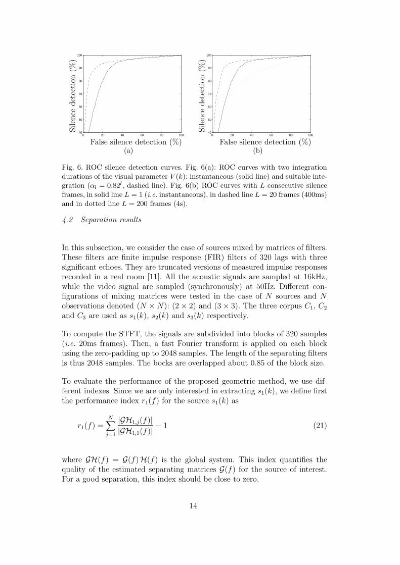
Fig. 6. ROC silence detection curves. Fig. 6(a): ROC curves with two integrationdurations of the visual parameter V (k): instantaneous (solid line) and suitable inte-gration (αl = 0.82l, dashed line). Fig. 6(b) ROC curves with L consecutive silenceframes, in solid line L = 1 (i.e. instantaneous), in dashed line L = 20 frames (400ms)and in dotted line L = 200 frames (4s).

4.2 Separation results

In this subsection, we consider the case of sources mixed by matrices of filters.These filters are finite impulse response (FIR) filters of 320 lags with threesignificant echoes. They are truncated versions of measured impulse responsesrecorded in a real room [11]. All the acoustic signals are sampled at 16kHz,while the video signal are sampled (synchronously) at 50Hz. Different con-figurations of mixing matrices were tested in the case of N sources and Nobservations denoted (N × N): (2 × 2) and (3 × 3). The three corpus C1, C2

and C3 are used as s1(k), s2(k) and s3(k) respectively.

To compute the STFT, the signals are subdivided into blocks of 320 samples(i.e. 20ms frames). Then, a fast Fourier transform is applied on each blockusing the zero-padding up to 2048 samples. The length of the separating filtersis thus 2048 samples. The bocks are overlapped about 0.85 of the block size.

To evaluate the performance of the proposed geometric method, we use dif-ferent indexes. Since we are only interested in extracting s1(k), we define firstthe performance index r1(f) for the source s1(k) as

r1(f) =N

∑

j=1

|GH1,j(f)|

|GH1,1(f)|− 1 (21)

where GH(f) = G(f)H(f) is the global system. This index quantifies thequality of the estimated separating matrices G(f) for the source of interest.For a good separation, this index should be close to zero.

14

Let w(k), y(k) and z(k) be three signals as z(k) = f(y(k))+w(k) where f(·) isa function. In the following (y|z)(k) denotes the contribution of y(k) in z(k):(y|z)(k) = f(y(k)). Moreover, let denote Py = 1

K

∑Kk=1 |y(k)|2 the average

power of signal y(k).

Thus, the signal to interference ratio (SIR) for the first source is defined as

SIR(s1|s†1) =

P(s1|s†1)

∑

sj 6=s1P(sj |s

†1)

. (22)

Note that (sj|s†1)(k) =

∑Ni=1 g1,i(k) ∗ hi,j(k) ∗ sj(k). This classical index in

source separation quantifies the quality of the estimated source s†1(k). For agood estimation of the source (i.e. ∀j > 1, (sj |s

†1)(k) ≃ 0), this index should

be close to infinity. Finally, we define the gain of the first source due to theseparation process as

G1 =SIR(s1|s

†1)

maxl SIR(s1|xl)

= minl

SIR(s1|s†1)

SIR(s1|xl)

(23)

with SIR(·|·) defined by (22) and (sj |xl)(k) = hl,j(k)∗sj(k). This gain allows toquantify the improvement in SIR before and after the separation process. (Thereference before separation being taken in the mixture where the contributionof s1(k) is the strongest.)

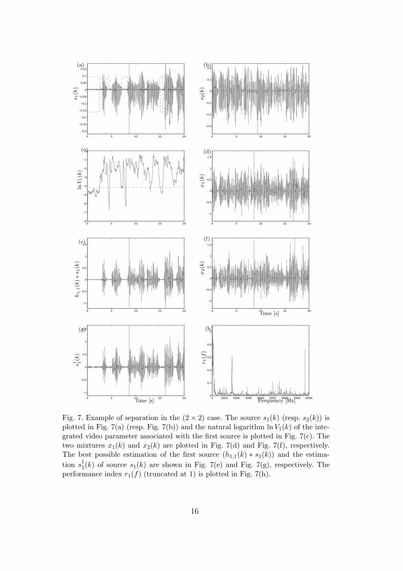
Fig. 7 presents a typical result of the separation process in the case of twosources and two sensors (2 × 2) with approximately a SIR for source s1(k)equal to 0 for both sensors. The two speech sources are plotted in Fig. 7(a)and Fig. 7(b). One can see on Fig. 7(c) ln V1(k), the natural logarithm of theintegrated video parameter (continuous line) and ln δ the natural logarithmof the threshold δ = 0.015 (dashdot line) used to estimate the silence frames(Section 2). In this example, and after the results of Section 2, the integrationcoefficients αl are equal to 0.82l and the minimal number of consecutive silenceframes L is chosen equal to 20 (i.e. the minimum length of a detected silenceis 400ms). The results of the V-VAD can be seen on Fig. 7(a): the framesmanually indexed as silence are represented by the dashdot line and the de-tected frames as silence (which define the estimation of T ) are representedby the dashed line. In this example 154 frames (i.e. 3.08s) were detected assilence representing 63.2% of silence detection while the false detection rateis only 1.3%. The two mixtures obtained from the two sources are plotted inFig. 7(d) and Fig. 7(f). The result s†1(k) of the extraction of source s1(k) bythe proposed method is shown in Fig. 7(g). As a reference, the best possibleestimation of the first source (h1,1(k) ∗ s1(k)) is plotted in Fig. 7(e). In thisexample, the gain G1 is equal to 17.4dB, while SIR(s1|s

†1) =18.4dB. One can

15

0 5 10 15 20

−0.3

−0.25

−0.2

−0.15

−0.1

−0.05

0

0.05

0.1

0.15

s1(k

)

(a)

0 5 10 15 20

−0.3

−0.2

−0.1

0

0.1

0.2

s2(k

)

(b)

0 5 10 15 20−8

−7

−6

−5

−4

−3

−2

−1

0

lnV1(k

)

(c)

0 5 10 15 20

−1

−0.5

0

0.5

1

1.5

x1(k

)

(d)

0 5 10 15 20

−1

−0.5

0

0.5

1

1.5

h1,1

(k)∗

s1(k

)

(e)

0 5 10 15 20

−1

−0.5

0

0.5

1

1.5

time [s]

x2(k

)

(f)

0 5 10 15 20

−1

−0.5

0

0.5

1

1.5

time [s]

s† 1(k

)

(g)

0 1000 2000 3000 4000 5000 6000 7000 80000

0.2

0.4

0.6

0.8

1

Frequency [Hz]

r1(f

)

(h)

Fig. 7. Example of separation in the (2 × 2) case. The source s1(k) (resp. s2(k)) isplotted in Fig. 7(a) (resp. Fig. 7(b)) and the natural logarithm ln V1(k) of the inte-grated video parameter associated with the first source is plotted in Fig. 7(c). Thetwo mixtures x1(k) and x2(k) are plotted in Fig. 7(d) and Fig. 7(f), respectively.The best possible estimation of the first source (h1,1(k) ∗ s1(k)) and the estima-

tion s†1(k) of source s1(k) are shown in Fig. 7(e) and Fig. 7(g), respectively. The

performance index r1(f) (truncated at 1) is plotted in Fig. 7(h).

16

−25 −20 −15 −10 −5 0 5 10 15 20 25−10

−5

0

5

10

15

20

25

G1

[dB

]

SIRin [dB](a)

−25 −20 −15 −10 −5 0 5 10 15 20 25−10

−5

0

5

10

15

20

25

G1

[dB

]

SIRin [dB](b)

Fig. 8. Expected gain G1 versus SIRin in the (2×2) (Fig. 8(a)) and (3×3) (Fig. 8(b))cases, respectively. The curves show the mean and the standard deviation of G1 indB.

see that the extraction of the first source is quite well performed. This is con-firmed by the index performance r1(f) (Fig. 7(h)): most values are close tozero.

Beyond this typical example, we processed extensive simulation tests. Foreach simulation, only 20 seconds of signals were used. Each configuration ofthe mixing matrices (N × N) and of the SIRin (where SIRin is the mean ofthe SIRs for each mixtures: SIRin = 1/N ×

∑

l SIR(s1|xl)) was run 50 timesand the presented results are given on average. To virtually create differentsource signals, each speech/acoustic signal is shifted randomly in time. Fig. 8presents the gain G1 versus the SIRin in both (2 × 2) and (3 × 3) cases.One can see that in both cases, the shape of the gains is the same: from lowSIRin (-20dB) to high SIRin (20dB), the gains are almost constant at a highvalue, demonstrating the efficiency of the proposed method: we obtain gainsof about 19dB in the (2 × 2) case and about 18dB in the (3 × 3) case. Then,the gains decrease to 11dB in the (2 × 2) case and to XXdB in the (3 × 3)case for higher SIRin. It is interesting to note that the gain can happen to benegative for the highest SIRin (e.g. (2×2) with SIRin = 20dB). However, thisis a rare situation since it happens only for isolated high ratio FA/BD (e.g.FA/BD > 15%), i.e. when the set T of detected silence frames contains toomuch frames for which s1(k) is active. Indeed in this case, a deeper analysisshows us that, since the average power of s1(k) is larger than the average powerof the other source(s) for high SIRin, the smallest eigenvalue of the covariancematrix estimated using this set T is not necessary associated with the firstsource. On the contrary, even if the ratio FA/BD is high while the SIRin

is low, the influence of interfering s1(k) values occurred during false alarmsremains poor because these values are small compared to the other source(s).Altogether, the method is efficient and reliable for a large range of SIRin

values (note that despite the previous remark, the smallest gain obtained atSIRin = 20dB for (2 × 2) mixture is about 11dB on the average).

17

5 Conclusion

In this paper, we proposed an efficient method which exploits the comple-mentarity of the bi-modality (audio/visual) of the speech signal. The visualmodality is used as a V-VAD, while the audio modality is used to estimatethe separation filter matrices exploiting detected silences of the source to beextracted. The proposed V-VAD has a major interest compared to audio onlyVAD: it is robust in any acoustic noise environment (e.g. in very low signalto noise ratio cases, in highly non-stationary environments with possibly mul-tiple interfering sources, etc.). Moreover, the proposed geometric separationprocess is based on the sparseness of the speech signal: when the source to beextracted is vanishing (i.e. during the silence frames given by the proposed V-VAD), the power of the corresponding estimated source is minimized thanksto the separating filters. The proposed method can be easily extended to ex-tract other/any sparse sources, using associated vanishing oracle. Note thatresults were presented for (2 × 2) and (3 × 3) mixtures but the method canbe applied to any arbitrary (N × N) mixture with N > 3. Also, compared toother frequency separation methods [7–11], the method has the strong advan-tage to intrinsically regularize the permutation problem: this regularizationis an inherent byproduct of the“smallest eigenvalue” search. Finally, we canconclude by underlining the low complexity of the method and low associatedcomputation cost, the video parameter extraction being set apart: comparedto the methods based on joint diagonalization of several matrices [7,11], theproposed method requires the simple diagonalization of one single covariancematrix.

Future works will mainly focus on the extraction of useful visual speechinformation in more natural conditions (e.g. lips without make-up, movingspeaker). Also, we intend to develop an on-line version of the geometric algo-rithm. These points are expected to allow the implementation of the proposedmethod for real environment and real-time applications.

References

[1] L. E. Bernstein, C. Benoıt, For speech perception by humans or machines, threesenses are better than one, in: Proc. Int. Conf. Spoken Language Processing(ICSLP), Philadelphia, USA, 1996, pp. 1477–1480.

[2] W. Sumby, I. Pollack, Visual contribution to speech intelligibility in noise, J.Acoust. Soc. Am. 26 (1954) 212–215.

[3] L. Girin, J.-L. Schwartz, G. Feng, Audio-visual enhancement of speech in noise,J. Acoust. Soc. Am. 109 (6) (2001) 3007–3020.

18

[4] D. Sodoyer, L. Girin, C. Jutten, J.-L. Schwartz, Developing an audio-visualspeech source separation algorithm, Speech Comm. 44 (1–4) (2004) 113–125.

[5] R. Dansereau, Co-channel audiovisual speech separation using spectralmatching constraints, in: Proc. IEEE Int. Conf. Acoustics, Speech, and SignalProcessing (ICASSP), Montreal, Canada, 2004.

[6] S. Rajaram, A. V. Nefian, T. S. Huang, Bayesian separation of audio-visualspeech sources, in: Proc. IEEE Int. Conf. Acoustics, Speech, and SignalProcessing (ICASSP), Montreal, Canada, 2004.

[7] B. Rivet, L. Girin, C. Jutten, Mixing audiovisual speech processing and blindsource separation for the extraction of speech signals from convolutive mixtures,IEEE Transactions on Speech and Audio Processing (Accepted for publication).

[8] V. Capdevielle, C. Serviere, J.-L. Lacoume, Blind separation of wide-bandsources in the frequency domain, in: Proc. IEEE Int. Conf. Acoustics, Speech,and Signal Processing (ICASSP), Detroit, USA, 1995, pp. 2080–2083.

[9] L. Para, C. Spence, Convolutive blind separation of non stationary sources,IEEE Transactions on Speech and Audio Processing 8 (3) (2000) 320–327.

[10] A. Dapena, M. F. Bugallo, L. Castedo, Separation of convolutive mixtures oftemporally-white signals: a novel frequency-domain approach, in: Proc. Int.Conf. Independent Component Analysis and Blind Source Separation (ICA),San Diego, USA, 2001, pp. 315–320.

[11] D.-T. Pham, C. Serviere, H. Boumaraf, Blind separation of convolutive audiomixtures using nonstationarity, in: Proc. Int. Conf. Independent ComponentAnalysis and Blind Source Separation (ICA), Nara, Japan, 2003.

[12] W. Wang, D. Cosker, Y. Hicks, S. Sanei, J. Chambers, Video assisted speechsource separation, in: Proc. IEEE Int. Conf. Acoustics, Speech, and SignalProcessing (ICASSP), Philadelphia, USA, 2005.

[13] P. Liu, Z. Wang, Voice activity detection using visual information, in: Proc.IEEE Int. Conf. Acoustics, Speech, and Signal Processing (ICASSP), Montreal,2004.

[14] J.-F. Cardoso, Blind signal separation: statistical principles, Proceedings of theIEEE 86 (10) (1998) 2009–2025.

[15] F. Abrard, Y. Deville, A time-frequency blind signal separation methodapplicable to underdetermined mixtures of dependent sources, Signal Processing85 (7) (2005) 1389–1403.

[16] M. Babaie-Zadeh, A. Mansour, C. Jutten, F. Marvasti, A geometric approachfor separating several speech signals, in: Proc. Int. Conf. IndependentComponent Analysis and Blind Source Separation (ICA), Granada, Spain, 2004,pp. 798–806.

[17] D. Sodoyer, B. Rivet, L. Girin, J.-L. Schwartz, C. Jutten, An analysis of visualspeech information applied to voice activity detection, in: Proc. IEEE Int. Conf.Acoustics, Speech, and Signal Processing (ICASSP), Toulouse, France, 2006.

19

[18] B. Le Goff, T. Guiard-Marigny, C. Benoıt, Read my lips... and my jaw! Howintelligible are the components of a speaker’s face?, in: Proc. Euro. Conf. onSpeech Com. and Tech, Madrid, Spain, 1995, pp. 291–294.

[19] F. Elisei, M. Odisio, G. Bailly, P. Badin, Creating and controlling video-realistictalking heads, in: Proc. Audio-Visual Speech Processing Workshop (AVSP),Aalborg, Denmark, 2001, pp. 90–97.

[20] T. Lallouache, Un poste visage-parole. Acquisition et traitement des contourslabiaux, in: Proc. Journees d’Etude sur la Parole (JEP) (French), Montreal,1990.

20