vibration-based monitoring and diagnostics using

Contents lists available at ScienceDirect

Journal of Sound and Vibration

Journal of Sound and Vibration 394 (2017) 612–630

http://d0022-46

☆ Thisn CorrE-m

journal homepage: www.elsevier.com/locate/jsvi

Vibration-based monitoring and diagnostics usingcompressive sensing$

Vaahini Ganesan a,n, Tuhin Das b, Nazanin Rahnavard c, Jeffrey L. Kauffman b

a Mech. & Aero. Engg. Dept., University of Central Florida, Orlando, FL, United Statesb Mech. & Aero. Engg. Dept., Univ. of Central Florida, Orlando, FL 32816, United Statesc Elec. & Comp. Engg. Dept., Univ. of Central Florida, Orlando, FL 32816, United States

a r t i c l e i n f o

Article history:Received 26 August 2016Received in revised form13 January 2017Accepted 1 February 2017Available online 12 February 2017

Keywords:Beam vibrationSparsityCompressive sensingFault detectionSignal recovery and reconstruction

x.doi.org/10.1016/j.jsv.2017.02.0020X/& 2017 Elsevier Ltd. All rights reserved.

work was supported by the National Scienesponding author.ail address: [email protected] (V

a b s t r a c t

Vibration data from mechanical systems carry important information that is useful forcharacterization and diagnosis. Standard approaches rely on continually streaming data ata fixed sampling frequency. For applications involving continuous monitoring, such asStructural Health Monitoring (SHM), such approaches result in high volume data and relyon sensors being powered for prolonged durations. Furthermore, for spatial resolution,structures are instrumented with a large array of sensors. This paper shows that bothvolume of data and number of sensors can be reduced significantly by applying Com-pressive Sensing (CS) in vibration monitoring applications. The reduction is achieved byusing random sampling and capitalizing on the sparsity of vibration signals in the fre-quency domain. Preliminary experimental results validating CS-based frequency recoveryare also provided. By exploiting the sparsity of mode shapes, CS can also enable efficientspatial reconstruction using fewer spatially distributed sensors. CS can thereby reduce thecost and power requirement of sensing as well as streamline data storage and processingin monitoring applications. In well-instrumented structures, CS can enable continuedmonitoring in case of sensor or computational failures.

& 2017 Elsevier Ltd. All rights reserved.

1. Introduction

Detecting and locating changes or faults in structures is an important field of research, as it has a direct impact on safetyand reliability. During their service lifetime, structural components undergo and accumulate change in characteristics [1].Early detection and location of these changes enable prolonged performance. In this regard, vibration-based monitoring is awell-established approach that is extensively documented in the literature [2]. Mechanical components such as shafts, windturbine blades, etc. inevitably undergo vibrations in their operating environment. These vibrations inherently carry sig-natures in temporal and spatial domains that help indicate and locate changes in their characteristics [3,4]. Vibration-baseddetection methods are also popular in civil engineering structures such as bridges [5–7], for monitoring their structuralhealth. A literature review of existing vibration-based monitoring and diagnostic techniques used in SHM is presented next.

Vibration-based SHM employs suitable in-situ active or passive transducers in order to analyze the characteristics of thestructure in time, frequency, and modal domains [8–12]. Earliest approaches to this type of SHM involved comparison of

ce Foundation under Grant ECCS-418710.

. Ganesan).

www.sciencedirect.com/science/journal/0022460X

www.elsevier.com/locate/jsvi

http://dx.doi.org/10.1016/j.jsv.2017.02.002



http://crossmark.crossref.org/dialog/?doi=10.1016/j.jsv.2017.02.002&domain=pdf



mailto:[email protected]


V. Ganesan et al. / Journal of Sound and Vibration 394 (2017) 612–630 613

modal properties of the damaged structure against an undamaged baseline of the same structure. Areas of applicationinclude structures such as bridges and wind turbines [4–6,13,14]. All vibration-based SHM methods rely heavily on time-history response of a structure that can be acquired using sensors such as accelerometers, strain gauges, etc. Modal para-meters are then extracted by transforming the response into frequency domain [15].

Looking more closely, detecting changes in the natural frequencies of a structure remains important in vibration-basedSHM [2]. It was shown that with increasing severity of damage, natural frequencies exhibited a more distributed shift asopposed to localized shift [10,16,17]. The effect of the geometry of damage on the shift was studied in [18,19]. Sensitivity offrequency shifts to damage and ambient variations has also been of interest [20,21]. In addition, experimental validationshave been conducted on actual structures [22–24]. Frequency Response Functions (FRF) have been utilized to determinenatural frequencies and their shifts [25–27]. Here, fault localization is suggested by collecting the FRF from multiple sensorsat different locations of the structure [8,28,29]. The review indeed confirms that while the shifting of natural frequencies is anindicator of structural change, it is not an effective means of locating the same. This brings the topic of spatial characterizationin SHM.

Mode shape extraction from the response of structures, for detection and localization of damage, is also popular [15,30].One technique is direct comparison between a specific mode shape of a structure in its healthy and damaged states usingeither Modal Assurance Criterion (MAC) or Coordinate Modal Assurance Criterion (COMAC) [31,32,14]. A disadvantage ofmode shapes based SHM is the large amount of data that is required in order to make reliable and accurate detection [8].Additionally, mode shape data is polluted by noise and measurement errors that affect their sensitivity to damage. A so-lution to by-pass this problem can be to measure the first (slope) or second (curvature) derivatives of the mode shape itself[33]. Nevertheless, the mode shape based SHM method is widely studied and applied in experiments as well [8,34–44]. Arelated method of extracting spatial information is by reconstructing the Operational Deflection Shapes (ODS) [45]. ODS aresuperposition of mode shapes and provide a physical view of the vibration of a structure [8,46]. Other approaches, such asthe use of transmissibility for detecting structural change [47], and use of correlation coefficients to distinguish strain data[48] have been explored in literature.

Other related techniques for structural monitoring include Guided Wave Testing (GWT) [49], imaging and pattern re-cognition [50], and Wavelet transforms [51–55]. Spatial wavelet analysis for damage detection and localization is a recentapproach that has gained popularity. However, inherent distortions in wavelet transform induces the possibility that da-mages near the boundaries of structures may be undetectable. In [56], the authors address this drawback by employing anovel padding method to the vibration response while using Continuous Wavelet Transform. While a plethora of techniquesare now available for SHM, they mostly involve instrumenting a given structure with as many sensors as possible. There-after, data extraction follows the traditional approach of Nyquist-Shannon's sampling theorem [57]. Advancements in sensorsystems and the drop in their costs have led to sensing proliferation, but at the expense of data volume, computationalburden and power-requirement [58].

As mechanical and civil engineering structures become more complicated and their performance standards are raised,monitoring and diagnostics will increasingly become more challenging. Hence, in spite of faster computational speeds andsuperior sensor technologies, it is imperative that the efficiency of condition monitoring be improved. Higher efficiency ofmonitoring implies reduced sensing requirement, low computational burden, and a greater flexibility of sensing. In [59], theauthors recognized the importance of down-sampling and investigated its effect on damage detection in the spatial domain.In this paper, the application of Compressive Sensing (CS) to vibration-based monitoring [60], is proposed in order toachieve reduced sensing. While this approach is still in its nascent stages, an important related work in literature is [61],where the authors evaluated the ability of CS to compress vibration data from civil structures. In [62], spatial interpolation ofthe impulse response of a vibrating plate using sub-nyquist sampling was investigated. Spatial sparsity may also beexploited for source localization of acoustic waves [63,64]. For data reduction, the combination of vibration-based mon-itoring and CS is optimal, since the former offers sparsity which the latter fundamentally requires. The approach is also lessreliant on mathematical modeling and model-based computations. This paper develops the foundation for CS basedmonitoring for lateral vibration of beams. Fundamentals of lateral beam vibrations and the effect of structural changes arediscussed in Section 2. Sparsity of vibrations and the motivation for using CS are discussed in Section 3. Examples of CS andquantitative comparison with Nyquist-Shannon sampling approach are given in Section 4. The use of CS in detecting changein natural frequencies is established and demonstrated through simulations in Section 5. Thereafter, spatial reconstructionof deflection-shape through CS and its application in locating a fault is shown in Section 6. Preliminary experimental va-lidation of CS for detecting shift in natural frequencies is presented in Section 7 using a cantilever beam setup. The quality ofspatial reconstruction is analyzed in Section 8. Finally concluding remarks with a note on future scope of this research aremade and references are provided.

2. Fundamental characteristics of beam vibrations

Fundamentals of beam vibration can be extended to analyzing vibration of practical mechanical structures. Hence, thestudy of beam vibrations is imperative and key to the development of the proposed research. The vibration characteristics ofbeams in their operating environment change with progression of faults or other introduced structural changes. In Sections2.1 and 2.2, we discuss the basics of beam vibrations and demonstrate changes in vibration characteristics through

V. Ganesan et al. / Journal of Sound and Vibration 394 (2017) 612–630614

simulations.

2.1. Lateral vibration response as weighted sum of modeshapes

The equation of motion of a uniform Euler-Bernoulli Beam is given by Eq. (1) [65]:

ρ∂ ( )∂

+ ∂ ( )∂

= ( ) ( )EIy x t

xA

y x tt

f x t, ,

, 1

4

4

2

2

where ( )y x t, is the lateral response of the beam, ( )f x t, represents forcing on the beam, E is the elastic modulus, I is thesecond moment of area, ρ is the density of the material and A is the area of cross section, all expressed in appropriate units.The response of the beam can be expressed as a weighted sum of its modeshapes as shown below,

∑( ) = ( ) ( )( )=

∞

y x t T t W x, .2q

q q1

Here, the qth mode is represented by its mode shape Wq(x), with principal co-ordinate Tq(t), attached to it. In its mostgeneral form, Tq(t) is influenced by both free and forced vibration components and can be expressed as [65]:

∫

∫ ∫

ω ωρ ω

τ ω τ τ( ) = ( ) + ( ) + ( ) ( ( − ))

= ( ) ( ) = ( ) ( )( )

T t A t B tAb

Q t d

b W x dx Q t f x t W x dx

cos sin1

sin

, ,3

q q q q qq

t

q n

L

q q

L

q

0

0

2

0

In Eq. (3), Aq and Bq are constants obtained from initial conditions, L is the length of the beam, and ωq is the qth naturalfrequency of vibration. Therefore, in effect, both free as well as forced vibration responses of a beam can be expressed as aweighted sum of mode shapes. Specifically, from Eqs. (2) and (3), the general structure of free vibration response of a beamis

⎡⎣ ⎤⎦ ⎡⎣ ⎤⎦∑ ∑ω ω ω ω( ) = ( ) + ( ) ( ) = ¯ ( ) ( ) + ¯ ( ) ( )( )=

∞

=

∞

y x t A t B t W x A x t B x t, cos sin cos sin ,4q

q q q q qq

q q q q1 1

where ¯ ( ) = ( )A x A W xq q q and ¯ ( ) = ( )B x B W xq q q . As expressed in Eq. (4), theoretically, the free vibration response of the beam is acombination of all its modes ( = …∞q 1, 2 ). However, given an initial deflection profile, ( )y x, 0 , the modes present in thatprofile are manifested in the response. Similarly, the steady response of a beam to harmonic forcing ω= ( )f f tsin f0 , applied atlocation x, takes the form

⎡⎣ ⎤⎦∑ ∑ω ω ω ω ω ω( ) = ( ) ( ) ( ) = ( ) ¯ ( ) ( )( )=

∞

=

∞

y x t D f t W x t D f W x, , sin sin , , .5q

q q f f q fq

q q f q1

01

0

The expression ω ω∑ ¯ ( ) ( )=∞ D f W x, ,q q q f q1 0 is the Operational Deflection Shape (ODS). The ODS is a constant shape that is

maintained at any time when the operational forcing frequency remains unchanged. Furthermore, it is a linear combinationof mode shapes Wq(x) and predominantly contains those modes that lie in close proximity to the forcing frequency. Vi-bration response of a beam carries two types of signatures, namely: (i) natural frequencies ωq in time domain, and (ii) modeshapes Wq(x) in the spatial domain. A change in a beam's characteristics, for instance due to damage or deterioration, causesthese signatures to change. Vibration-based monitoring of structures rely on detecting and quantifying these changes.Section 2.2 illustrates how structural changes or faults are manifested in natural frequencies, mode shapes and the ODS.

2.2. Identifying structural change using vibrational signatures

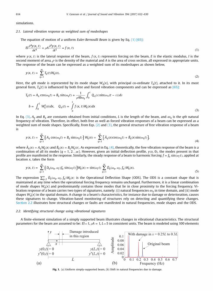
A finite-element simulation of a simply supported beam illustrates changes in vibrational characteristics. The structuralparameters for the beam are assumed to be: EI¼1, ρ =A 1, L¼5 in consistent units. The beam is modeled using 100 elements

Fig. 1. (a) Uniform simply-supported beam, (b) Shift in natural frequencies due to damage.

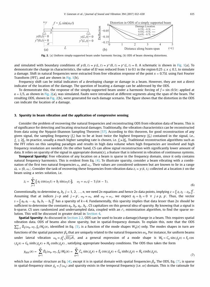
Fig. 2. (a) Uniform simply-supported beam under harmonic forcing, (b) ODS of beam showing distortions.


and simulated with boundary conditions of ( ) = ( ) = ″( ) = ″( ) =y t y L t y t y L t0, , 0, , 0. A schematic is shown in Fig. 1(a). Todemonstrate the change in characteristics, the value of EI was reduced from 1 to 0.1 in the region ≤ ≤x0.25 0.3, to simulatea damage. Shift in natural frequencies were extracted from free vibration response of the point =x L0.75 using Fast FourierTransform (FFT), and are shown in Fig. 1(b).

Frequency shift can be initial indicators of a developing change or damage in a beam. However, they are not a directindicator of the location of the damage. The question of locating a damage can be addressed by the ODS.

To demonstrate this, the response of the simply-supported beam under a harmonic forcing of = ( )f tsin 0.5 applied at=a L/5, as shown in Fig. 2(a), was simulated. Faults were introduced at different segments along the span of the beam. The

resulting ODS, shown in Fig. 2(b), were generated for each damage scenario. The figure shows that the distortion in the ODScan indicate the location of a damage.

3. Sparsity in beam vibration and the application of compressive sensing

Consider the problem of recovering the natural frequencies and reconstructing ODS from vibration data of beams. This isof significance for detecting and locating structural damages. Traditionally, the vibration characteristics can be reconstructedfrom data using the Nyquist-Shannon Sampling Theorem [57]. According to this theorem, for good reconstruction of anygiven signal, the sampling frequency (fs) has to be at least twice the highest frequency (fb) contained in the signal, i.e.,

≥f f2s b. In practice, usually a much higher sampling rate is chosen, i.e. ⪢f f2s b. Traditional reconstruction algorithms such asthe FFT relies on this sampling paradigm and results in high data volume when high frequencies are involved and highfrequency resolution are needed. On the other hand, CS can allow signal reconstruction with significantly lower amount ofdata. It relies on sparsity of the signal in appropriate domain(s), a feature that is inherent in vibration of continuous systems.

Temporal Sparsity: Free vibration of any location on a beam is sparse in the frequency domain, since it only containsnatural frequency harmonics. This is evident from Eq. (4). To illustrate sparsity, consider a beam vibrating with a combi-nation of the first two natural frequencies ωα and ωγ . Their values are considered unknown but are known to lie in a rangeΩ ω= [ ]0,r r . Consider the task of recovering these frequencies from vibration data = ( ¯ )z y x t,i i collected at a location x on thebeam using a series solution, i.e.

⎡⎣ ⎤⎦∑ ω ω ω ω= ( ) + ( ) = ( − ) ( − )( )=

z a t b t j ncos sin , 1 / 1 .6

ij

n

j j j j j r1

Conventionally, to determine aj, bj, = …j n1, 2, , , we need n2 equations and hence n2 data points, implying ⎡⎣ ⎤⎦= ⋯z z z z nT

1 2 2 .Assuming that at indices j¼p and = ′j p , ω ω= αp and ω ω= γ′p , we expect = = ∀ ≠ ′a b j p p0 ,j j . Thus, the vector

⎡⎣ ⎤⎦= ⋯ ⋯s a a a b b bn nT

0 1 0 1 has a sparsity of k¼4. Fundamentally, this sparsity implies that data lesser than n2 should besufficient to determine the constants ′ ′a b a b, , ,p p p p . CS capitalizes on this general idea of sparsity. By knowing that a signal isk-sparse, CS uses randomized and undersampled data, coupled with an ℓ1 minimization algorithm, to find the sparse so-lution. This will be discussed in greater detail in Section 4.

Spatial Sparsity: As discussed in Section 2.2, ODS can be used to locate a damage/change in a beam. This requires spatialvibration data. ODS of beams also show sparsity, but in spatial-frequency domain. To explain this, note that the ODS

ω ω∑ ¯ ( ) ( )=∞ D f W x, ,q q q f q1 0 , identified in Eq. (5), is a function of the mode shapes Wq(x) only. The modes shapes in turn are

functions of the spatial parameter βq that are uniquely related to the natural frequenciesωq. For instance, for uniform beams

under lateral vibration ω β ρ= EI A/q q2 , and a general expression of a mode shape is β= ( ) +W C x Fsin cosq q q q

β β β( ) + ( ) + ( )x G x H xsinh coshq q q q q , satisfying appropriate boundary conditions. The ODS thus takes the form

∑ ∑ω ω β β β β( ) = ¯ ( ) ( ) = ¯ ( ) + ¯ ( ) + ¯ ( ) + ¯ ( )( )=

∞

=

∞

y x D f W x C x F x G x H x, , sin cos sinh cosh ,7

ODSq

q q f qq

q q q q q q q q1

01

which has a similar structure as Eq. (4), except it is in spatial domain with spatial frequencies βq. The ODS, Eq. (7), is sparsein spatial-frequency since β ω= ( )fq q and sparsity exists in the temporal frequency (i.e. ω) domain. This is the rationale for


applying CS to ODS reconstruction, which amounts to requiring fewer spatially distributed sensors. In addition to the ODS,free vibration of beams also shows spatial sparsity. This can be shown from Eq. (4). However, the deflection shape of freevibration varies with time. Thus, ODS is deemed a preferred candidate for spatial reconstruction, and for comparison withbaseline data to locate faults.

4. Compressive sensing (CS)

4.1. An example of CS

CS deals with frequency recovery and reconstruction of an under-sampled signal from random, linear and non-adaptivemeasurements when the signal is sparsely represented in a proper basis [60]. The CS problem refers to finding a sparsesolution ∈s Rn, with sparsity k (i.e. with ≤k nonzero entries), of the equation

Φ = ( )s z, 8

given a vector of measurements ∈z Rm and a measurement matrix Φ ∈ ×Rm n with <m n. The sparsest solution of theaforementioned under-determined set of equations is obtained from the l0 minimization of s, which is NP-Hard to compute[60]. An alternative that is less computationally intensive is the ℓ1 minimization of s, which is given as

Φ^ = ∥ ∥ = ( )ℓs argmin s s z: subject to , 91

where ∥ ∥ = ∑ | |ℓ =s sin

i11 . The equivalence of the ℓ1 solution to ℓ0 is guaranteed under an additional condition on Φ, namely theRestricted Isometry Property (RIP) [66], which will be discussed in Section 4.2. The ℓ1 minimization is a convex optimizationproblem [67], and therefore easier to solve computationally. When the number of measurements m is of the order [68],

( )≃ ( ) ( )m O k ln n k/ , 10

a carefully designed Φ satisfies RIP of order k2 , thus allowing for the sparse solution to be obtained with overwhelming prob-ability. In Eq. (10), k is the number of non-zero entries in s and hence represents its sparsity. While this result was originallyderived for randommatrices mostly, CS maybe extended to recovery of signals that have other types of expansions as well [68]. Inthe application to beam vibration, Φ is determined based on the beam response equation in temporal and spatial domains.

An example of frequency recovery using compressive sampling, from a given signal in time domain, is discussed next.Consider a signal y(t) that can be expressed as ω( ) = ∑ ( )=y t a tsini

ni i1 . Further, assume that the vector = [ ⋯ ]s a a an

T1 2 is k-

sparse, i.e. only ( < )k n entries of s are non-zero. Let the corresponding frequency range for y be denoted by Ω ω ω∈ [ ],n n1 .The CS problem, Eq. (8), can be posed as: find the k-sparse solution s from m measurements of y, i.e. from = ( )z y tj j , where

= ⋯j m1, 2, . The vector = [ ⋯ ]z z z zmT

1 2 consists of measurements made at random instants, and Φ ∈ ×Rm n is constructed asΦ ω= ( )tsinj i i j, . A lower bound on m is obtained from Eq. (10). Thus, Eq. (8) takes the form

⎡

⎣

⎢⎢⎢

⎤

⎦

⎥⎥⎥

⎡

⎣

⎢⎢⎢⎢

⎤

⎦

⎥⎥⎥⎥

⎡

⎣

⎢⎢⎢

⎤

⎦

⎥⎥⎥Φ

ω ω ωω ω ω

ω ω ω

= ⇒ ⋮ =

( ) ( ) ⋯ ( )( ) ( ) ⋯ ( )⋮ ⋮ ⋯ ⋮

( ) ( ) ⋯ ( )⋮z s

zz

z

t t t

t t t

t t t

aa

a

sin sin sinsin sin sin

sin sin sin

.

m

n

n

m m n m n

1

2

1 1 2 1 1

1 2 2 2 2

1 2

1

2

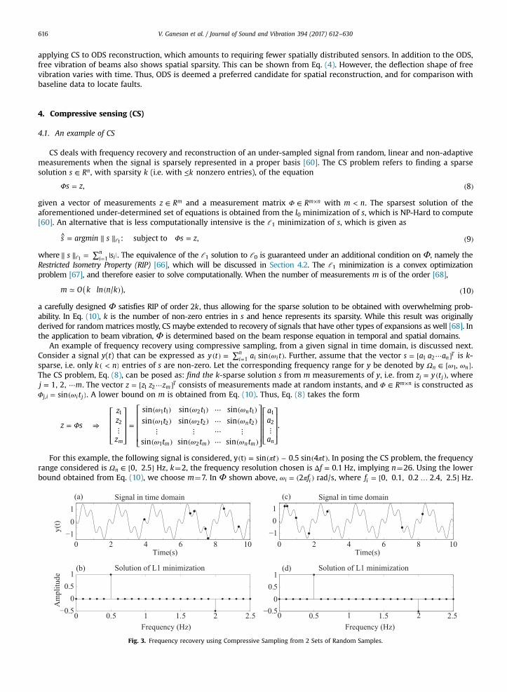
For this example, the following signal is considered, π π( ) = ( ) − ( )t ty t sin 0.5 sin 4 . In posing the CS problem, the frequencyrange considered is Ω ∈ [ ]0, 2.5 Hzn , k¼2, the frequency resolution chosen is Δ =f 0.1 Hz, implying n¼26. Using the lowerbound obtained from Eq. (10), we choose m¼7. In Φ shown above, ω π= ( )f2 rad/si i , where = [ … ]f 0, 0.1, 0.2 2.4, 2.5 Hzi .

Fig. 3. Frequency recovery using Compressive Sampling from 2 Sets of Random Samples.


Fig. 3 illustrates two trials of frequency recovery using random sampling. The first trial is shown in Figs. 3(a) and (b), whilethe second one is depicted in Figs. 3(c) and (d). In each trial, the samples are randomly chosen and the ℓ1 minimization iscarried out using the ℓ1-magic code [69]. It can be observed that the desired frequencies are recovered at exact amplitudesin both the trials, irrespective of sample distribution. As mentioned above, the design ofΦ is important for CS to be effective.To this end, Φ must satisfy a Restricted Isometry Property, explained in the next section.

4.2. Restricted isometry property (RIP)

The reconstruction of an under-sampled signal requires the design of a suitable measurement matrix Φ and that thesignal be represented in a proper basis where it is k-sparse. For a high probability of reconstruction, Φ needs to satisfy theRestricted Isometry Property (RIP). A matrix Φ is said to satisfy RIP of order k if its Restricted Isometric Constant δk satisfies

δ< <0 1k . The constant δk is defined as the smallest value satisfying

δ Φ δ( − ) ≤ ∥ ∥∥ ∥

≤ ( + )( )

vv

1 1 ,11

k k22

22

for all vectors v with sparsity ≤k [60]. Satisfying the RIP implies that all the column sub-matrices ofΦ are well conditioned.These attributes lead to high probability of signal recovery by CS [60,66]. For a given k, δk for a matrix Φ ∈ ×Rm n can bedetermined numerically by applying the condition

δ λ Φ Φ λ Φ Φ δ( − ) ≤ ( ′ ) ≤ ( ′ ) ≤ ( + ) ( )1 1 12k min T T max T T k

for all sub-matrices Φ ∈ ×RTm p that can be formed from any p columns ofΦ, with ≤ ≤p k1 . In practice, however, δ ≥ 1k is not

forbidden; it would simply mean that the stability of recovery under noise and the closeness of the ℓ1 solution to ℓ0 solutionmay not be well guaranteed [70].

In order to quantify RIP better, consider the example of Section 4.1. Since k¼2 in this example, we need to determine δ2.For the given m�n (7�26) Φ matrix, we determined δ = 0.952 . Thus δ < 12 , and frequency recovery was reliable with highprobability. Increasing the number of measurements m to 20 yielded δ = 0.632 , which is expected. A lower δ2 implies ahigher probability of accurate frequency recovery. A third scenario, with n¼16 and m¼7, yielded δ = 0.842 .

4.3. Quantitative comparison of CS and nyquist-shannon sampling theorem

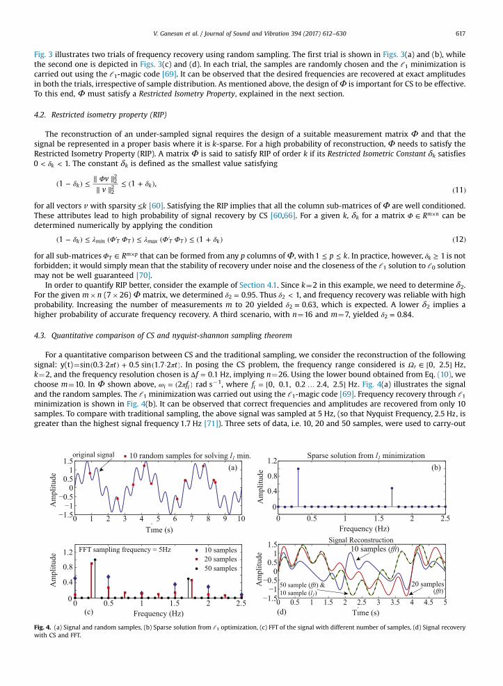
For a quantitative comparison between CS and the traditional sampling, we consider the reconstruction of the followingsignal: y(t)¼ π π( · ) + ( · )t tsin 0.3 2 0.5 sin 1.7 2 . In posing the CS problem, the frequency range considered is Ω ∈ [ ]0, 2.5 Hzr ,k¼2, and the frequency resolution chosen is Δ =f 0.1 Hz, implying n¼26. Using the lower bound obtained from Eq. (10), wechoose m¼10. In Φ shown above, ω π= ( )f2i i rad s�1, where = [ … ]f 0, 0.1, 0.2 2.4, 2.5 Hzi . Fig. 4(a) illustrates the signaland the random samples. The ℓ1 minimization was carried out using the ℓ1-magic code [69]. Frequency recovery through ℓ1minimization is shown in Fig. 4(b). It can be observed that correct frequencies and amplitudes are recovered from only 10samples. To compare with traditional sampling, the above signal was sampled at 5 Hz, (so that Nyquist Frequency, 2.5 Hz, isgreater than the highest signal frequency 1.7 Hz [71]). Three sets of data, i.e. 10, 20 and 50 samples, were used to carry-out

Fig. 4. (a) Signal and random samples, (b) Sparse solution from ℓ1 optimization, (c) FFT of the signal with different number of samples, (d) Signal recoverywith CS and FFT.


DFT (using the FFT algorithm). The consequent signal reconstruction in each of the three cases is achieved using thosefrequency components whose amplitudes are significantly above the noise level. The results are shown in Fig. 4(c) and (d).While the ℓ1 minimization gave accurate reconstruction with 10 samples, the reconstruction had significant errors whentraditional sampling technique was used, even with 20 samples. The accuracy of ℓ1-based reconstruction with 10 samples isat the same level as that of the reconstruction from FFT components with 50 samples.

The main differences between CS and FFT based approaches are:1. Uniform vs. Random Sampling: The random sampling in CS effectively allows the data to be richer in information

with fewer samples compared to regular sampling in FFT. In FFT this richness is achieved by increasing frequency andduration of sampling.

2. Exact vs. Probabilistic Solution: The FFT solution is exact in the sense that the quantity of data and the number ofunknowns match. In contrast, ℓ1 optimization fundamentally relies on sparsity and solves an under-determined systemiteratively. This, combined with randomness of data, can assure recovery with a certain probability, albeit a very high one ifRIP is satisfied by Φ.

3. Volume of Data: FFT fundamentally relies on high sampling rate for recovering a wide frequency-band and relies onhigh sampling duration for obtaining adequate resolution between neighboring frequencies. Both individually increase thedata requirement proportionally. In CS, the data requirement is considerably more moderate, since it increases only withsparsity and in a logarithmic manner with the number of frequency components in Φ, Eq. (10).

4. Signal Sparsity: The ℓ1 optimization relies on sparsity, and hence for sparse signals CS out-performs FFT. If signalsparsity is weak, the two methods may show comparable performance.

5. Frequency recovery from beam vibration

In Section 2.2, free vibration response of a beam was discussed, changes in natural frequencies and ODS were noted forchanges in structural characteristics, and the sparsity of spatio-temporal vibration was discussed. This section explores thefeasibility of using reduced number of (randomly placed) samples to recover the natural frequencies of vibration of me-chanical beams using CS. This is investigated under two conditions: (i) When no changes have been introduced (unmodifiedor baseline) (ii) After changes have been introduced in the structure (modified). The following sections develop this methodfor simply supported and cantilever beams.

5.1. Detecting natural frequencies of a simply supported beam using CS

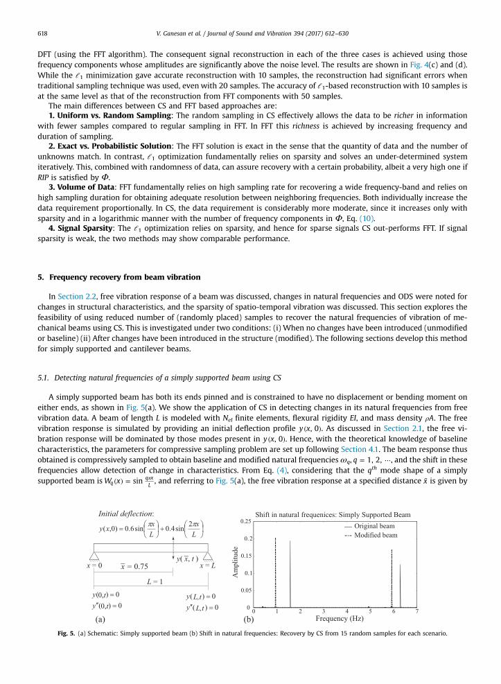
A simply supported beam has both its ends pinned and is constrained to have no displacement or bending moment oneither ends, as shown in Fig. 5(a). We show the application of CS in detecting changes in its natural frequencies from freevibration data. A beam of length L is modeled with Nel finite elements, flexural rigidity EI, and mass density ρA. The freevibration response is simulated by providing an initial deflection profile ( )y x, 0 . As discussed in Section 2.1, the free vi-bration response will be dominated by those modes present in ( )y x, 0 . Hence, with the theoretical knowledge of baselinecharacteristics, the parameters for compressive sampling problem are set up following Section 4.1. The beam response thusobtained is compressively sampled to obtain baseline and modified natural frequenciesωq, = ⋯q 1, 2, , and the shift in thesefrequencies allow detection of change in characteristics. From Eq. (4), considering that the qth mode shape of a simplysupported beam is ( ) = πW x sinq

q xL, and referring to Fig. 5(a), the free vibration response at a specified distance x is given by

Fig. 5. (a) Schematic: Simply supported beam (b) Shift in natural frequencies: Recovery by CS from 15 random samples for each scenario.


∑ ∑

∑

ω ω ω ω π

ω ω

( ¯ ) = ( ( ) + ( )) ( ¯) = ( ( ) + ( ))¯

= ( ¯ ( ¯) ( ) + ¯ ( ¯) ( ))( )

=

∞

=

∞

=

∞

y x t A t B t W x A t B tq x

L

A x t B x t

, cos sin cos sin sin

cos sin ,13

qq q q q q

qq q q q

qq q q q

1 1

1

where ¯ ( ¯) = π ¯A x A sinq qq x

Land ¯ ( ¯) = π ¯B x B sinq q

q xL. The measurement point, x, is chosen such that it does not fall at the nodal

point (zero displacement point) of the response. In a realistic scenario, since multiple sensors will be spatially distributed, ifa sensor location coincides with a node, alternate sensors can be used for CS based recovery. Consider the goal of recoveringthe natural frequencies ωq using CS, within a frequency range of Ω ω∈ [ ]0,r r . Further, consider a frequency recovery re-solution ωΔ . The measurement vector ∈z Rm is generated from m random measurements = ( ¯ )z y x t,j j , = ⋯j m1, 2, , and thematrix Φ is constructed using sine and cosine basis functions, Eq. (13). Since each frequency is represented by two basisfunctions, we expect even-sparsity in the solution of ⎡⎣ ⎤⎦= ′ ′ ⋯ ′ ′ ′ ⋯ ′s A A A B B Bn n

T1 2 1 2 , ω ω= ( Δ ) +n / 1r , obtained from the

ℓ1 minimum solution of Eq. (8). In this case, Eq. (8) takes the form

⎡

⎣

⎢⎢⎢

⎤

⎦

⎥⎥⎥

⎡

⎣

⎢⎢⎢⎢

⎤

⎦

⎥⎥⎥⎥

⎡⎣ ⎤⎦

Φ

ω ω ω ωω ω ω ω

ω ω ω ω

= ⇒ ⋮ =

( ) ⋯ ( ) ( ) ⋯ ( )( ) ⋯ ( ) ( ) ⋯ ( )⋮ ⋮ ⋮ ⋮ ⋮ ⋮

( ) ⋯ ( ) ( ) ⋯ ( )

= ⋯ ⋯ ( )′ ′ ′ ′ ′ ′

z s

zz

z

t t t t

t t t t

t t t t

s

s A A A B B B

cos cos sin sincos cos sin sin

cos cos sin sin

where . 14

m

n n

n n

m n m m n m

n nT

1

2

1 1 1 1 1 1

1 2 2 1 2 2

1 1

1 2 1 2

In Eq. (14), ωi, with = …i n1, 2, , , represent the spanning frequencies of the rangeΩr, i.e. ω ω= Δ ( − )i 1i , ω = 01 and ω ω=n r .The ℓ1 minimum sparse solution is referred to as s , Eq. (9).

To demonstrate CS, a simply supported beam is considered with the following specifications: L¼1, ρ =A 1, EI¼1. Thenatural frequencies ωq are ⎡⎣ ⎤⎦π π π ⋯, 4 , 92 2 2 in rad/s, and the corresponding mode shapes are ⎡⎣ ⎤⎦π π π( ) ( ) ( ) ⋯x x xsin , sin 2 , sin 3 ,[65]. Free vibration is simulated using a discrete model consisting of =N 500el beam elements. It is given an initial deflectionprofile of π π( ) = ( ) + ( )y x x L x L, 0 0.6 sin / 0.4 sin 2 / , which is a combination of the first two mode shapes. This causes the firsttwo natural frequencies to be manifested in the free vibration response. Typically, the proposed method can be applied to awide variety of initial conditions and the corresponding modes will be manifested in the response. Change is introduced byreducing EI from 1 to 0.1 in the segment ≤ ≤L x L0.4 0.5 . The time domain response of the beam, before and after change, ismeasured at ¯ =x L3 /4. The ℓ1 minimization problem of Eq. (14) is setup with ω π= =7 Hz 14 rad/sr and

ω πΔ = =0.01 Hz 0.02 rad/s. This yields n¼701 and we choose m¼15 random measurements. This is comparable to m¼20suggested by Eq. (10), which is based on a sparsity of four for the first two natural frequencies. Note that the frequency rangeΩ ∈ [ ]0, 7 is chosen to cover the first two natural frequencies ω π π= /2 Hz, 2 Hzq .

The solutions of the two ℓ1 minimization problems, namely before and after making changes in EI, are shown in Fig. 5. Aschematic of the beam is shown in Fig. 5(a). Frequency recovery from data collected at ¯ = =x L3 /4 0.75 is shown in Fig. 5(b).The original natural frequencies ω π π= /2 Hz, 2 Hzq are correctly predicted by the ℓ1 minimum solution. The amplitudes

plotted are +′ ′A Bi i2 2 , since each frequency ωi has a combined basis function ⎡⎣ ⎤⎦ω ω′ ( ) + ′ ( )A t B tsin cosi i i i , as evident from

Eqs. (13) and (14). Fig. 5(b) also shows the shift in frequencies due to the change in EI. They were also determined by solvingthe same ℓ1 minimization problem. The reduction in frequencies is expected since change was introduced in the form ofreduction in EI (stiffness/rigidity).

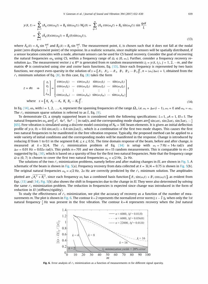
To study the effectiveness of ℓ1 minimization, we plot the accuracy of recovery as a function of the number of mea-surementsm. The plot is shown in Fig. 6. The contour k¼2 represents the normalized error norm∥ − ^ ∥s s 2 when only the 1stnatural frequency π Hz

2was present in the free vibration. The contour k¼4 represents recovery when the 2nd natural

Fig. 6. Error analysis of ℓ1 minimization as a function of measurements m for different signal sparsity.

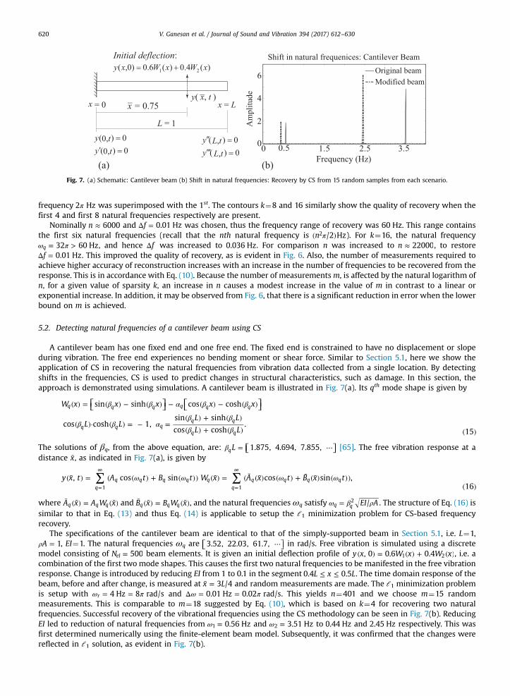
Fig. 7. (a) Schematic: Cantilever beam (b) Shift in natural frequencies: Recovery by CS from 15 random samples from each scenario.


frequency π2 Hz was superimposed with the 1st. The contours k¼8 and 16 similarly show the quality of recovery when thefirst 4 and first 8 natural frequencies respectively are present.

Nominally ≈n 6000 and Δ =f 0.01 Hz was chosen, thus the frequency range of recovery was 60 Hz. This range containsthe first six natural frequencies (recall that the nth natural frequency is π( )n /2 Hz2 ). For k¼16, the natural frequencyω π= >32 60 Hzq , and hence Δf was increased to 0.036 Hz. For comparison n was increased to ≈n 22000, to restoreΔ =f 0.01 Hz. This improved the quality of recovery, as is evident in Fig. 6. Also, the number of measurements required toachieve higher accuracy of reconstruction increases with an increase in the number of frequencies to be recovered from theresponse. This is in accordance with Eq. (10). Because the number of measurementsm, is affected by the natural logarithm ofn, for a given value of sparsity k, an increase in n causes a modest increase in the value of m in contrast to a linear orexponential increase. In addition, it may be observed from Fig. 6, that there is a significant reduction in error when the lowerbound on m is achieved.

5.2. Detecting natural frequencies of a cantilever beam using CS

A cantilever beam has one fixed end and one free end. The fixed end is constrained to have no displacement or slopeduring vibration. The free end experiences no bending moment or shear force. Similar to Section 5.1, here we show theapplication of CS in recovering the natural frequencies from vibration data collected from a single location. By detectingshifts in the frequencies, CS is used to predict changes in structural characteristics, such as damage. In this section, theapproach is demonstrated using simulations. A cantilever beam is illustrated in Fig. 7(a). Its qth mode shape is given by

⎡⎣ ⎤⎦ ⎡⎣ ⎤⎦β β α β β

β β αβ ββ β

( ) = ( ) − ( ) − ( ) − ( )

( )· ( ) = − =( ) + ( )( ) + ( ) ( )

W x x x x x

L LL L

L L

sin sinh cos cosh

cos cosh 1,sin sinh

cos cosh.

15

q q q q q q

q q qq q

q q

The solutions of βq, from the above equation, are: ⎡⎣ ⎤⎦β = ⋯L 1.875, 4.694, 7.855,q [65]. The free vibration response at adistance x, as indicated in Fig. 7(a), is given by

∑ ∑ω ω ω ω( ¯ ) = ( ( ) + ( )) ( ¯) = ( ¯ ( ¯) ( ) + ¯ ( ¯) ( ))( )=

∞

=

∞

y x t A t B t W x A x t B x t, cos sin cos sin ,16q

q q q q qq

q q q q1 1

where ¯ ( ¯) = ( ¯)A x A W xq q q and ¯ ( ¯) = ( ¯)B x B W xq q q , and the natural frequencies ωq satisfy ω β ρ= EI A/q q2 . The structure of Eq. (16) is

similar to that in Eq. (13) and thus Eq. (14) is applicable to setup the ℓ1 minimization problem for CS-based frequencyrecovery.

The specifications of the cantilever beam are identical to that of the simply-supported beam in Section 5.1, i.e. L¼1,ρ =A 1, EI¼1. The natural frequencies ωq are ⎡⎣ ⎤⎦⋯3.52, 22.03, 61.7, in rad/s. Free vibration is simulated using a discretemodel consisting of =N 500el beam elements. It is given an initial deflection profile of ( ) = ( ) + ( )y x W x W x, 0 0.6 0.41 2 , i.e. acombination of the first two mode shapes. This causes the first two natural frequencies to be manifested in the free vibrationresponse. Change is introduced by reducing EI from 1 to 0.1 in the segment ≤ ≤L x L0.4 0.5 . The time domain response of thebeam, before and after change, is measured at ¯ =x L3 /4 and random measurements are made. The ℓ1 minimization problemis setup with ω π= =4 Hz 8 rad/sr and ω πΔ = =0.01 Hz 0.02 rad/s. This yields n¼401 and we choose m¼15 randommeasurements. This is comparable to m¼18 suggested by Eq. (10), which is based on k¼4 for recovering two naturalfrequencies. Successful recovery of the vibrational frequencies using the CS methodology can be seen in Fig. 7(b). ReducingEI led to reduction of natural frequencies from ω = 0.56 Hz1 and ω = 3.51 Hz2 to 0.44 Hz and 2.45 Hz respectively. This wasfirst determined numerically using the finite-element beam model. Subsequently, it was confirmed that the changes werereflected in ℓ1 solution, as evident in Fig. 7(b).


6. Reconstruction of deflection shapes using CS

Section 2.2 illustrates that changes in beam characteristics produce distortions in its ODS. Determining the spatial re-sponse or the ODS is key to locating these changes. This section investigates reconstruction of the ODS of a beam using CS byapplying it spatially. The deflection shape of a beam under free vibration, at an instant t , can be expressed in terms of thenormal modes = ⋯∞q 1, 2, as

∑

∑

ω ω( ¯) = [ ( ¯) + ( ¯)] ( )

= (¯) ( )( )

=

∞

=

∞

y x t A t B t W x

C t W x

, cos sin

,17

qq q q q q

qq q

1

1

where ω ω(¯) = [ ( ¯) + ( ¯)]C t A t B tcos sinq q q q q and Wq is the qth mode shape. On the other hand, the steady response of a beam toharmonic forcing ω= ( )f f tsin f0 , applied at location x takes the form of Eq. (5). From Eqs. (17) and (5), one distinction of thetwo deflection shapes is that the former is dependent on t , while the other is not, provided the forcing has a steadyamplitude and frequency. The latter represents the ODS. It is time-invariant and will be the focus of deflection re-construction. The rationale for formulating the deflection shape reconstruction using compressive-sensing is that modeshapes Wq are sparse in βq, since βq and ωq are related by ω β ρ= EI A/q q

2 . For instance for a simply-supported beam,

β= = πW xsin sinq qq x

Land that for a cantilever beam are given by Eq. (15). The following sections explain and illustrate ℓ1

minimum solutions for reconstructing deflection shapes for simply-supported, fixed-fixed and cantilever beams. The em-phasis will be on reconstruction from forced vibration response.

6.1. Deflection shape reconstruction for simply supported beam

Spatial recovery remains essentially similar to that of time-domain frequency recovery. The only difference being,sampling of the beam response is performed at one time instant from different spatial points along the length of the beam.In essence, the length axis becomes analogous to time axis. The parameters used to define the beam, L, EI and ρA, are thesame as those in Section 5.1. Results of CS based recovery are validated against a finite-element model of the beam of Nel

elements. Fig. 8(a) illustrates the beam. From Eq. (5), the deflection equation for a simply supported beam can be expressedas

∑ β π( ¯) = ¯ (¯) = ( ) =( )=

∞

y x t D t W W xq x

L, , sin sin .

18qq q q q

1

Thus, the basis functions are sinusoids of wavelengths λ = L q2 /q , i.e. of spatial frequency ξ = q L/2q . Consider the problem ofreconstructing the deflection shape of the beam under a harmonic force with frequency ω ω ω< < +q f q 1. The deflection shapewill be dominated by the qth and ( + )q 1 th mode shapes, i.e. by ξq and ξqþ1. Consider a spatial frequency range ⎡⎣ ⎤⎦Ξ ξ ξ= ,r l h ,such that ξ ξ Ξ( ) ∈+,q q r1 , and a measurement vector ∈z Rm generated by measurements y taken at m random locations alongthe length of the beam at an instant t , = ( ¯)z y x t,j j , = ⋯j m1, 2, . Writing zj as

∑ πξ ξ ξ ξ ξ= ( ) = + ( − ) ( − )−

= ⋯( )

z H x in

i nsin 2 , 11

, 1, 2, ,19

ji

n

i i j i lh l

the deflection shape can be reconstructed by determining the ℓ1 minimum solution of

Fig. 8. (a) Schematic: Simply Supported beam with harmonic excitation (b) Spatial frequencies recovered before and after modification of elements.

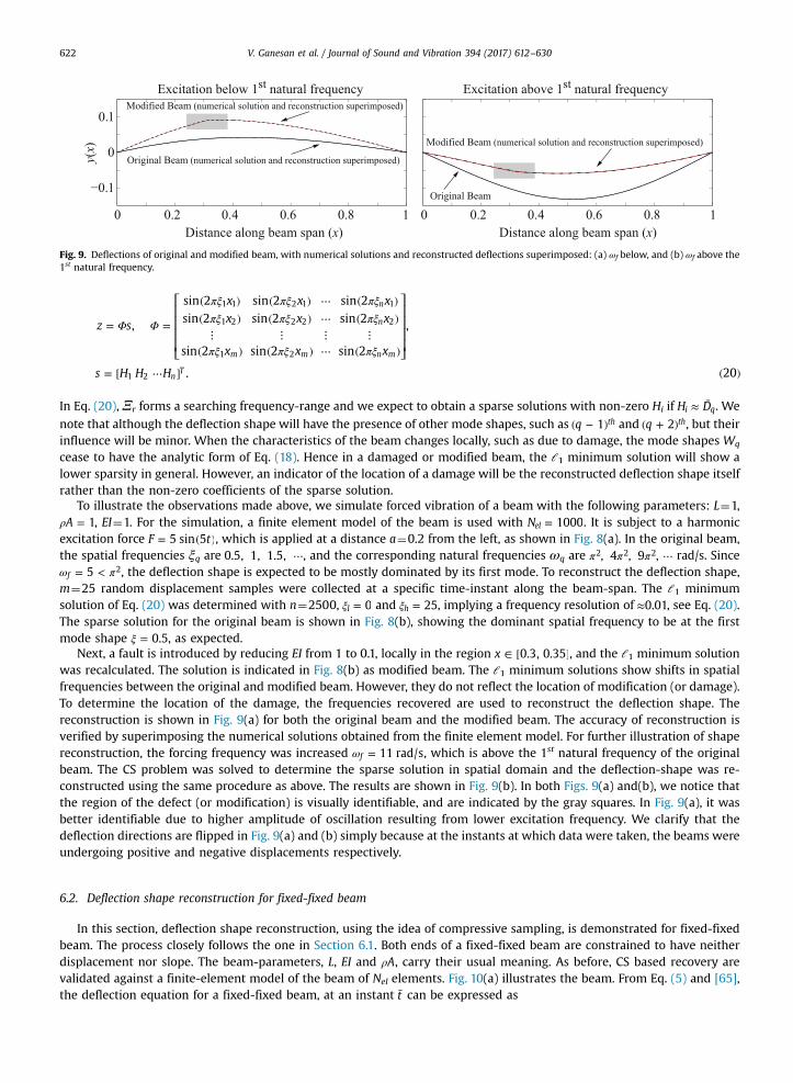
Fig. 9. Deflections of original and modified beam, with numerical solutions and reconstructed deflections superimposed: (a) ωf below, and (b) ωf above the1st natural frequency.


⎡

⎣

⎢⎢⎢⎢

⎤

⎦

⎥⎥⎥⎥

Φ Φ

πξ πξ πξπξ πξ πξ

πξ πξ πξ

= =

( ) ( ) ⋯ ( )( ) ( ) ⋯ ( )

⋮ ⋮ ⋮ ⋮( ) ( ) ⋯ ( )

= [ ⋯ ] ( )

z s

x x x

x x x

x x x

s H H H

,

sin 2 sin 2 sin 2sin 2 sin 2 sin 2

sin 2 sin 2 sin 2

,

. 20

n

n

m m n m

nT

1 1 2 1 1

1 2 2 2 2

1 2

1 2

In Eq. (20), Ξr forms a searching frequency-range and we expect to obtain a sparse solutions with non-zero Hi if ≈ ¯H Di q. We

note that although the deflection shape will have the presence of other mode shapes, such as ( − )q 1 th and ( + )q 2 th, but theirinfluence will be minor. When the characteristics of the beam changes locally, such as due to damage, the mode shapes Wq

cease to have the analytic form of Eq. (18). Hence in a damaged or modified beam, the ℓ1 minimum solution will show alower sparsity in general. However, an indicator of the location of a damage will be the reconstructed deflection shape itselfrather than the non-zero coefficients of the sparse solution.

To illustrate the observations made above, we simulate forced vibration of a beam with the following parameters: L¼1,ρ =A 1, EI¼1. For the simulation, a finite element model of the beam is used with =N 1000el . It is subject to a harmonicexcitation force = ( )F t5 sin 5 , which is applied at a distance a¼0.2 from the left, as shown in Fig. 8(a). In the original beam,the spatial frequencies ξq are ⋯0.5, 1, 1.5, , and the corresponding natural frequencies ωq are π π π ⋯, 4 , 9 ,2 2 2 rad/s. Sinceω π= <5f

2, the deflection shape is expected to be mostly dominated by its first mode. To reconstruct the deflection shape,m¼25 random displacement samples were collected at a specific time-instant along the beam-span. The ℓ1 minimumsolution of Eq. (20) was determined with n¼2500, ξ = 0l and ξ = 25h , implying a frequency resolution of ≈0.01, see Eq. (20).The sparse solution for the original beam is shown in Fig. 8(b), showing the dominant spatial frequency to be at the firstmode shape ξ = 0.5, as expected.

Next, a fault is introduced by reducing EI from 1 to 0.1, locally in the region ∈ [ ]x 0.3, 0.35 , and the ℓ1 minimum solutionwas recalculated. The solution is indicated in Fig. 8(b) as modified beam. The ℓ1 minimum solutions show shifts in spatialfrequencies between the original and modified beam. However, they do not reflect the location of modification (or damage).To determine the location of the damage, the frequencies recovered are used to reconstruct the deflection shape. Thereconstruction is shown in Fig. 9(a) for both the original beam and the modified beam. The accuracy of reconstruction isverified by superimposing the numerical solutions obtained from the finite element model. For further illustration of shapereconstruction, the forcing frequency was increased ω = 11 rad/sf , which is above the 1st natural frequency of the originalbeam. The CS problem was solved to determine the sparse solution in spatial domain and the deflection-shape was re-constructed using the same procedure as above. The results are shown in Fig. 9(b). In both Figs. 9(a) and(b), we notice thatthe region of the defect (or modification) is visually identifiable, and are indicated by the gray squares. In Fig. 9(a), it wasbetter identifiable due to higher amplitude of oscillation resulting from lower excitation frequency. We clarify that thedeflection directions are flipped in Fig. 9(a) and (b) simply because at the instants at which data were taken, the beams wereundergoing positive and negative displacements respectively.

6.2. Deflection shape reconstruction for fixed-fixed beam

In this section, deflection shape reconstruction, using the idea of compressive sampling, is demonstrated for fixed-fixedbeam. The process closely follows the one in Section 6.1. Both ends of a fixed-fixed beam are constrained to have neitherdisplacement nor slope. The beam-parameters, L, EI and ρA, carry their usual meaning. As before, CS based recovery arevalidated against a finite-element model of the beam of Nel elements. Fig. 10(a) illustrates the beam. From Eq. (5) and [65],the deflection equation for a fixed-fixed beam, at an instant t can be expressed as

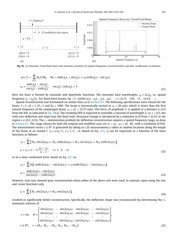
Fig. 10. (a) Schematic: Fixed-fixed beam with harmonic excitation (b) Spatial frequencies recovered before and after modification of elements.


∑ β β α β β

αβ β

β ββ β

( ¯) = ¯ (¯) = ( − ) + ( − )

=−

−=

( )

=

∞

y x t D t W W x x x x

L L

L LL L

, , sinh sin cosh cos ,

sinh sin

cos cosh, cos . cosh 1.

21

qq q q q q q q q

qq q

q qq q

1

Here the basis is formed by sinusoids and hyperbolic functions. The sinusoids have wavelengths λ π β= 2 /q q, i.e. spatialfrequency ξ β π= /2q q . For fixed-fixed beams, Eq. (21) yields β β β β[ ⋯] = [ ⋯]L L L L, , , , 4.73, 7.85, 11, 14.14,1 2 3 4 .

Spatial reconstruction was formulated on similar lines as in Section 6.1. The following specifications were chosen for thebeam: L¼1, ρ =A 1, EI¼1 and =N 1000el . The beam is harmonically excited at ω = 20 rad/sf which is lower than the firstnatural frequency of the undamaged beam, ω β= = 22.37 rad/s1 1

2 . The force, of amplitude 5, is applied at a distance a¼0.2from the left, as indicated in Fig. 10(a). The resulting ODS is expected to resemble a sinusoid of wavelength 2, i.e. ξ = 0.5, butwith zero deflection and slope near the fixed ends. Structural change is introduced by a reduction in EI from 1 to 0.1 in theregion ∈ [ ]x 0.3, 0.35 . The ℓ1 minimization problem for deflection reconstruction requires a spatial frequency range, as donein Section 6.1. The range chosen for both the original and modified cases are Ξ ξ ξ= [ ] = [ ], 0, 40r l h , with a resolution of 0.01.The measurement vector ∈z Rm is generated by taking m¼25 measurements y taken at random locations along the lengthof the beam at an instant t , = ( ¯)z y x t,j j , = ⋯j m1, 2, . Based on Eq. (21), zj can be expressed as a function of the basisfunctions as follows:

⎡⎣ ⎤⎦∑ πξ πξ πξ πξ

ξ ξ ξ ξ

= ( ) + ( ) + ( ) + ( )

= + ( − ) ( − )−

= ⋯ ( )

z H x H x H x H x

in

i n

sin 2 sinh 2 cos 2 cosh 2 ,

11

, 1, 2, , 22

ji

n

i i j i i j i i j i i j

i lh l

,1 ,2 ,3 ,4

or in a more condensed form, based on Eq. (21) as,

⎡⎣ ⎤⎦∑ πξ πξ α πξ πξ

α πξ πξπξ πξ

= ( ( ) − ( )) + ( ( ) − ( ))

= ( ) − ( )( ) − ( ) ( )

z H x x x x

L LL L

sinh 2 sin 2 cosh 2 cos 2

sinh 2 sin 2cos 2 cosh 2

.23

ji

n

i i j i j i i j i j

ii i

i i

However, trial runs showed poor reconstruction when either of the above sets were used. In contrast, upon using the sineand cosine functions only

⎡⎣ ⎤⎦∑ πξ πξ= ( ) + ( )( )

z H x H xsin 2 cos 2 ,24

ji

n

i i j i i j,1 ,2

resulted in significantly better reconstruction. Specifically, the deflection shape was reconstructed by determining the ℓ1minimum solution of

⎡

⎣

⎢⎢⎢⎢

⎤

⎦

⎥⎥⎥⎥

Φ Φ

πξ πξ πξ πξπξ πξ πξ πξ

πξ πξ πξ πξ

= =

( ) ⋯ ( ) ( ) ⋯ ( )( ) ⋯ ( ) ( ) ⋯ ( )

⋮ ⋮ ⋮ ⋮ ⋮ ⋮( ) ⋯ ( ) ( ) ⋯ ( )

∈ = [ ⋯ ⋯ ] ( )

z s

x x x x

x x x x

x x x x

z R s H H H H H H

,

sin 2 sin 2 cos 2 cos 2sin 2 sin 2 cos 2 cos 2

sin 2 sin 2 cos 2 cos 2

,

, . 25

n n

n n

m n m m n m

mn n

T

1 1 1 1 1 1

1 2 2 1 2 2

1 1

1,1 2,1 ,1 1,2 2,2 ,2

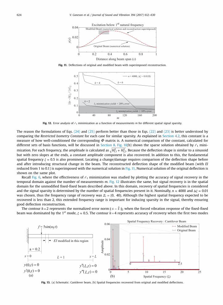
Fig. 11. Deflections of original and modified beam with superimposed reconstruction.

Fig. 12. Error analysis of ℓ1 minimization as a function of measurements m for different spatial signal sparsity.


The reason the formulations of Eqs. (24) and (25) perform better than those in Eqs. (22) and (23) is better understood bycomparing the Restricted Isometry Constant for each case for similar sparsity. As explained in Section 4.2, this constant is ameasure of how well-conditioned the corresponding Φ matrix is. A numerical comparison of the constant, calculated fordifferent sets of basis functions, will be discussed in Section 8. Fig. 10(b) shows the sparse solution obtained by ℓ1 mini-

mization. For each frequency, the amplitude is calculated as +H Hi i,12

,22 . Because the deflection shape is similar to a sinusoid

but with zero slopes at the ends, a constant amplitude component is also recovered. In addition to this, the fundamentalspatial frequency ξ = 0.5 is also prominent. Locating a change/damage requires comparison of the deflection shape beforeand after introducing structural change in the beam. The reconstructed deflection shape of the modified beam (with EIreduced from 1 to 0.1) is superimposed with the numerical solution in Fig. 11. Numerical solution of the original deflection isshown on the same plot.

Recall Fig. 6, where the effectiveness of ℓ1 minimization was studied by plotting the accuracy of signal recovery in thetemporal domain against the number of measurements m. Fig. 12 illustrates the same, but signal recovery is in the spatialdomain for the unmodified fixed-fixed beam described above. In this domain, recovery of spatial frequencies is consideredand the signal sparsity is determined by the number of spatial frequencies present in it. Nominally, ≈n 4000 and ξΔ = 0.01was chosen, thus the frequency range of recovery was Ξ = [ ]0, 40r . Although the highest spatial frequency expected to berecovered is less than 2, this extended frequency range is important for inducing sparsity in the signal, thereby ensuringgood deflection reconstruction.

The contour k¼2 represents the normalized error norm ∥ − ^ ∥s s 2 when the forced vibration response of the fixed-fixedbeam was dominated by the 1st mode, ξ ≈ 0.5. The contour k¼4 represents accuracy of recovery when the first two modes

Fig. 13. (a) Schematic: Cantilever beam, (b) Spatial frequencies recovered from original and modified deflections.

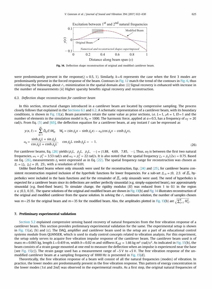
Fig. 14. Deflection shape reconstruction of original and modified cantilever beam.


were predominantly present in the response(ξ ≈ 0.5, 1). Similarly, k¼6 represents the case when the first 3 modes arepredominantly present in the forced response of the beam. Contours in Fig. 12 match the trend of the contours in Fig. 6, thusreinforcing the following about ℓ1 minimization in the spatial domain also: (i) Signal recovery is enhanced with increase inthe number of measurements (ii) Higher sparsity benefits signal recovery and reconstruction.

6.3. Deflection shape reconstruction for cantilever beam

In this section, structural changes introduced in a cantilever beam are located by compressive sampling. The processclosely follows that explained in the Sections 6.1 and 6.2. A schematic representation of a cantilever beam, with its boundaryconditions, is shown in Fig. 13(a). Beam parameters retain the same value as prior sections, i.e. L¼1, ρ =A 1, EI¼1 and thenumber of elements in the simulation model is =N 1000el . The harmonic force, applied at a¼0.5, has a frequency of ω = 20f

rad/s. From Eq. (5) and [65], the deflection equation for a cantilever beam, at any instant t can be expressed as

∑ β β α β β

αβ β

β ββ β

( ¯) = ¯ (¯) = ( − ) − ( − )

=+

+= −

( )

=

∞

y x t D t W W x x x x

L L

L LL L

, , sin sinh cos cosh ,

sinh sin

cos cosh, cos . cosh 1.

26

qq q q q q q q q

qq q

q qq q

1

For cantilever beams, Eq. (26) yields β β β[ ⋯] = [ ⋯]L L L, , , 1.88, 4.69, 7.85,1 2 3 . Thus, ωf is between the first two naturalfrequencies, ω β= = 3.53 rad/s1 1

2 and ω β= = 22 rad/s2 22 . It is also noted that the spatial frequency ξ β π= ( ) =/ 2 0.752 2 . Based

on Eq. (26), measurements zj were expressed as in Eq. (22). The spatial frequency range for reconstruction was chosen asΞ ξ ξ= [ ] = [ ], 0, 25r l h , with a resolution of 0.01.

Unlike fixed-fixed beams where only sinusoids were used for the reconstruction, Eqs. (24) and (25), for cantilever beams con-sistent reconstruction required inclusion of the hyperbolic functions for lower frequencies. For a sub-set Ξ = [ ]0, 2.5r h, of Ξr, hy-

perbolics were included in the basis functions and for the remainder of Ξr, only sinusoids were used. The need of hyperbolics isexpected for a cantilever beam since its deflections are neither perfectly sinusoidal (e.g. simply-supported beam), nor approximatelysinusoidal (e.g. fixed-fixed beam). To simulate change, the rigidity modulus (EI) was reduced from 1 to 0.1 in the region

∈ [ ]x 0.3, 0.35 . The sparse solutions of the original andmodified beam are shown in Fig. 13(b) and Fig. 14 illustrates reconstruction ofthe original and modified cantilever from the sparse solution. In solving the ℓ1 minimum solution, the number of samples chosen

was m¼25 for the original beam and m¼35 for the modified beam. Also, the amplitudes plotted in Fig. 13(b) are ∑ = Hj i j14

,2 .

7. Preliminary experimental validation

Section 5.2 explained compressive sensing based recovery of natural frequencies from the free vibration response of acantilever beam. This section provides preliminary experimental validation for the same. The experimental setup is shownin Fig. 15(a), (b) and (c). The DAQ, amplifier and cantilever beam used in the setup are a part of an educational controlsystems module from QUANSER, which is used to study control concepts related to vibration analysis. For this experiment,the setup solely serves to acquire free vibration impulse response of the cantilever beam. The cantilever beam used is ofmass m¼0.065 kg, length L¼0.419 m, width b¼0.02 m and stiffness = ( )K 1.66 kg m rad/sstiff

2 2. As indicated in Fig. 15(b), thebeam consists of a strain gauge mounted at one end to measure the deflection when an impulse is experienced near the base(see Fig. 15(c)). The strain gauge used has a measurement range of −5 V to +5 V . The free vibration response of the un-modified cantilever beam at a sampling frequency of 1000 Hz is presented in Fig. 15(d).

Theoretically, the free vibration response of a beam will consist of all the natural frequencies (modes) of vibration. Inpractice, the lower modes are predominantly present in the free vibration response. This pattern of energy concentration inthe lower modes (1st and 2nd) was observed in the experimental results. As a first step, the original natural frequencies of

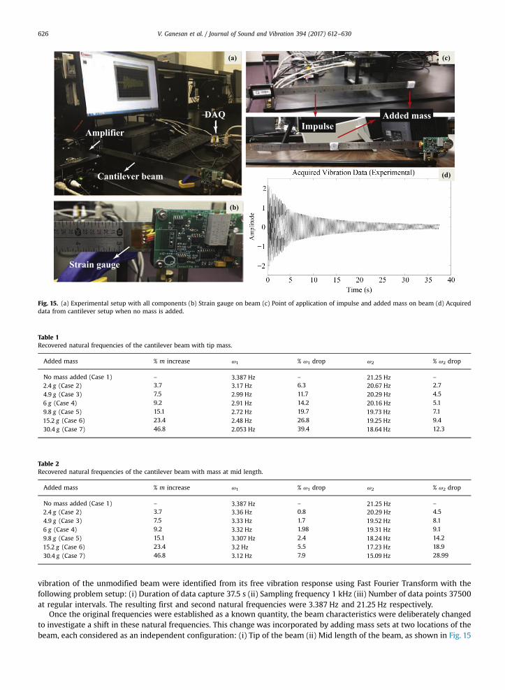
Fig. 15. (a) Experimental setup with all components (b) Strain gauge on beam (c) Point of application of impulse and added mass on beam (d) Acquireddata from cantilever setup when no mass is added.

Table 1Recovered natural frequencies of the cantilever beam with tip mass.

Added mass % m increase ω1 % ω1 drop ω2 % ω2 drop

No mass added (Case 1) – 3.387 Hz – 21.25 Hz –

g2.4 (Case 2) 3.7 3.17 Hz 6.3 20.67 Hz 2.7

g4.9 (Case 3) 7.5 2.99 Hz 11.7 20.29 Hz 4.5

g6 (Case 4) 9.2 2.91 Hz 14.2 20.16 Hz 5.1

g9.8 (Case 5) 15.1 2.72 Hz 19.7 19.73 Hz 7.1

g15.2 (Case 6) 23.4 2.48 Hz 26.8 19.25 Hz 9.4

g30.4 (Case 7) 46.8 2.053 Hz 39.4 18.64 Hz 12.3

Table 2Recovered natural frequencies of the cantilever beam with mass at mid length.

Added mass % m increase ω1 % ω1 drop ω2 % ω2 drop

No mass added (Case 1) – 3.387 Hz – 21.25 Hz –

g2.4 (Case 2) 3.7 3.36 Hz 0.8 20.29 Hz 4.5

g4.9 (Case 3) 7.5 3.33 Hz 1.7 19.52 Hz 8.1

g6 (Case 4) 9.2 3.32 Hz 1.98 19.31 Hz 9.1

g9.8 (Case 5) 15.1 3.307 Hz 2.4 18.24 Hz 14.2

g15.2 (Case 6) 23.4 3.2 Hz 5.5 17.23 Hz 18.9

g30.4 (Case 7) 46.8 3.12 Hz 7.9 15.09 Hz 28.99


vibration of the unmodified beam were identified from its free vibration response using Fast Fourier Transform with thefollowing problem setup: (i) Duration of data capture 37.5 s (ii) Sampling frequency 1 kHz (iii) Number of data points 37500at regular intervals. The resulting first and second natural frequencies were 3.387 Hz and 21.25 Hz respectively.

Once the original frequencies were established as a known quantity, the beam characteristics were deliberately changedto investigate a shift in these natural frequencies. This change was incorporated by adding mass sets at two locations of thebeam, each considered as an independent configuration: (i) Tip of the beam (ii) Mid length of the beam, as shown in Fig. 15

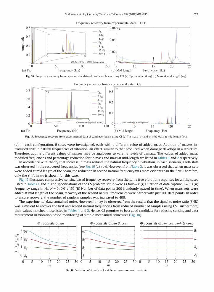
Fig. 16. Frequency recovery from experimental data of cantilever beam using FFT (a) Tip mass (ω1 & ω2) (b) Mass at mid length (ω2).

Fig. 17. Frequency recovery from experimental data of cantilever beam using CS (a) Tip mass (ω1 and ω2) (b) Mass at mid length (ω2).


(c). In each configuration, 6 cases were investigated, each with a different value of added mass. Addition of masses in-troduced shift in natural frequencies of vibration, an effect similar to that produced when damage develops in a structure.Therefore, adding different values of masses may be analogous to varying levels of damage. The values of added mass,modified frequencies and percentage reduction for tip mass and mass at mid-length are listed in Tables 1 and 2 respectively.

In accordance with theory that increase in mass reduces the natural frequency of vibration, in each scenario, a left-shiftwas observed in the recovered frequencies (see Fig. 16 (a), (b)). However, from Table 2, it was observed that when mass setswere added at mid length of the beam, the reduction in second natural frequency was more evident than the first. Therefore,only the shift in ω2 is shown for this case.

Fig. 17 illustrates compressive sensing based frequency recovery from the same free vibration responses for all the caseslisted in Tables 1 and 2. The specifications of the CS problem setup were as follows: (i) Duration of data capture −0 5 s (ii)Frequency range in Hz, =N 0: 0.01: 150 (ii) Number of data points 200 (randomly spaced in time). When mass sets wereadded at mid length of the beam, recovery of the second natural frequencies were harder with just 200 data points. In orderto ensure recovery, the number of random samples was increased to 400.

The experimental data contained noise. However, it may be observed from the results that the signal to noise ratio (SNR)was sufficient to recover the first and second natural frequencies from reduced number of samples using CS. Furthermore,their values matched those listed in Tables 1 and 2. Hence, CS promises to be a good candidate for reducing sensing and datarequirement in vibration based monitoring of simple mechanical structures (Fig. 18).

Fig. 18. Variation of δk with m for different measurement matrix Φ.


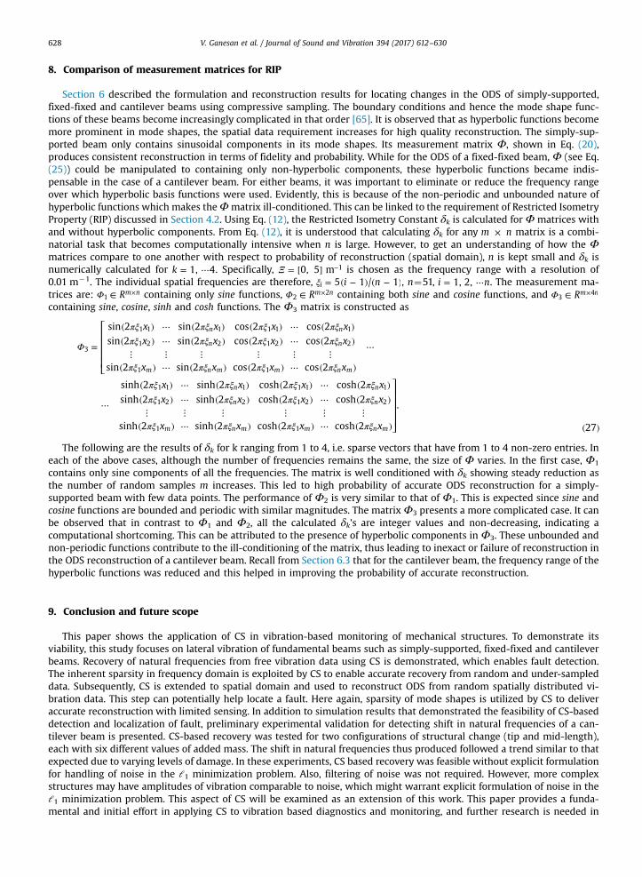
8. Comparison of measurement matrices for RIP

Section 6 described the formulation and reconstruction results for locating changes in the ODS of simply-supported,fixed-fixed and cantilever beams using compressive sampling. The boundary conditions and hence the mode shape func-tions of these beams become increasingly complicated in that order [65]. It is observed that as hyperbolic functions becomemore prominent in mode shapes, the spatial data requirement increases for high quality reconstruction. The simply-sup-ported beam only contains sinusoidal components in its mode shapes. Its measurement matrix Φ, shown in Eq. (20),produces consistent reconstruction in terms of fidelity and probability. While for the ODS of a fixed-fixed beam, Φ (see Eq.(25)) could be manipulated to containing only non-hyperbolic components, these hyperbolic functions became indis-pensable in the case of a cantilever beam. For either beams, it was important to eliminate or reduce the frequency rangeover which hyperbolic basis functions were used. Evidently, this is because of the non-periodic and unbounded nature ofhyperbolic functions which makes theΦmatrix ill-conditioned. This can be linked to the requirement of Restricted IsometryProperty (RIP) discussed in Section 4.2. Using Eq. (12), the Restricted Isometry Constant δk is calculated forΦ matrices withand without hyperbolic components. From Eq. (12), it is understood that calculating δk for any ×m n matrix is a combi-natorial task that becomes computationally intensive when n is large. However, to get an understanding of how the Φmatrices compare to one another with respect to probability of reconstruction (spatial domain), n is kept small and δk isnumerically calculated for = ⋯k 1, 4. Specifically, Ξ = [ ] −0, 5 m 1 is chosen as the frequency range with a resolution of0.01 m�1. The individual spatial frequencies are therefore, ξ = ( − ) ( − )i n5 1 / 1i , n¼51, = ⋯i n1, 2, . The measurement ma-trices are: Φ ∈ ×Rm n

1 containing only sine functions, Φ ∈ ×Rm n2

2 containing both sine and cosine functions, and Φ ∈ ×Rm n3

4

containing sine, cosine, sinh and cosh functions. The Φ3 matrix is constructed as

⎡

⎣

⎢⎢⎢⎢

⎤

⎦

⎥⎥⎥⎥

Φ


πξ πξ πξ πξ


πξ πξ πξ πξ

=

( ) ⋯ ( ) ( ) ⋯ ( )( ) ⋯ ( ) ( ) ⋯ ( )

⋮ ⋮ ⋮ ⋮ ⋮ ⋮( ) ⋯ ( ) ( ) ⋯ ( )

⋯

⋯

( ) ⋯ ( ) ( ) ⋯ ( )( ) ⋯ ( ) ( ) ⋯ ( )

⋮ ⋮ ⋮ ⋮ ⋮ ⋮( ) ⋯ ( ) ( ) ⋯ ( ) ( )

x x x x

x x x x

x x x x

x x x x

x x x x

x x x x

sin 2 sin 2 cos 2 cos 2sin 2 sin 2 cos 2 cos 2

sin 2 sin 2 cos 2 cos 2

sinh 2 sinh 2 cosh 2 cosh 2sinh 2 sinh 2 cosh 2 cosh 2

sinh 2 sinh 2 cosh 2 cosh 2

.

27

n n

n n

m n m m n m

n n

n n

m n m m n m

3

1 1 1 1 1 1

1 2 2 1 2 2

1 1

1 1 1 1 1 1

1 2 2 1 2 2

1 1

The following are the results of δk for k ranging from 1 to 4, i.e. sparse vectors that have from 1 to 4 non-zero entries. Ineach of the above cases, although the number of frequencies remains the same, the size of Φ varies. In the first case, Φ1

contains only sine components of all the frequencies. The matrix is well conditioned with δk showing steady reduction asthe number of random samples m increases. This led to high probability of accurate ODS reconstruction for a simply-supported beam with few data points. The performance of Φ2 is very similar to that of Φ1. This is expected since sine andcosine functions are bounded and periodic with similar magnitudes. The matrixΦ3 presents a more complicated case. It canbe observed that in contrast to Φ1 and Φ2, all the calculated δk's are integer values and non-decreasing, indicating acomputational shortcoming. This can be attributed to the presence of hyperbolic components in Φ3. These unbounded andnon-periodic functions contribute to the ill-conditioning of the matrix, thus leading to inexact or failure of reconstruction inthe ODS reconstruction of a cantilever beam. Recall from Section 6.3 that for the cantilever beam, the frequency range of thehyperbolic functions was reduced and this helped in improving the probability of accurate reconstruction.

9. Conclusion and future scope

This paper shows the application of CS in vibration-based monitoring of mechanical structures. To demonstrate itsviability, this study focuses on lateral vibration of fundamental beams such as simply-supported, fixed-fixed and cantileverbeams. Recovery of natural frequencies from free vibration data using CS is demonstrated, which enables fault detection.The inherent sparsity in frequency domain is exploited by CS to enable accurate recovery from random and under-sampleddata. Subsequently, CS is extended to spatial domain and used to reconstruct ODS from random spatially distributed vi-bration data. This step can potentially help locate a fault. Here again, sparsity of mode shapes is utilized by CS to deliveraccurate reconstruction with limited sensing. In addition to simulation results that demonstrated the feasibility of CS-baseddetection and localization of fault, preliminary experimental validation for detecting shift in natural frequencies of a can-tilever beam is presented. CS-based recovery was tested for two configurations of structural change (tip and mid-length),each with six different values of added mass. The shift in natural frequencies thus produced followed a trend similar to thatexpected due to varying levels of damage. In these experiments, CS based recovery was feasible without explicit formulationfor handling of noise in the ℓ1 minimization problem. Also, filtering of noise was not required. However, more complexstructures may have amplitudes of vibration comparable to noise, which might warrant explicit formulation of noise in theℓ1 minimization problem. This aspect of CS will be examined as an extension of this work. This paper provides a funda-mental and initial effort in applying CS to vibration based diagnostics and monitoring, and further research is needed in


many fronts. Combined spatio-temporal CS, optimized sensor placement, extension to complicated structures, and im-proved robustness of recovery/reconstruction, are some of the future directions to be pursued.

References

[1] Z.Y. Shi, S.S. Law, L.M. Zhang, Structural damage detection from modal strain energy change, J. Eng. Mech. 126 (12) (2000) 1216–1223.[2] S.W. Doebling, C.R. Farrar, M.B. Prime, D.W. Shevitz, Damage identification and health monitoring of structural and mechanical systems from changes

in their vibration characteristics: A literature review, Tech. rep., Los Alamos National Lab., NM, USA, 1996.[3] N. Tandon, A. Choudhury, A review of vibration and acoustic measurement methods for the detection of defects in rolling element bearings, Tribol. Int.

32 (8) (1999) 469–480.[4] A. Ghoshal, M.J. Sundaresan, M.J. Schulz, P.F. Pai, Structural health monitoring techniques for wind turbine blades, J. Wind Eng. Ind. Aerodyn. 85 (3)

(2000) 309–324.[5] A.E. Aktan, F.N. Catbas, K.A. Grimmelsman, C.J. Tsikos, Issues in infrastructure health monitoring for management, J. Eng. Mech. 126 (7) (2000) 711–724.[6] F.N. Catbas, A.E. Aktan, Condition and damage assessment: issues and some promising indices, J. Struct. Eng. 128 (8) (2002) 1026–1036.[7] F.N. Catbas, H.B. Gokce, M. Gul, Nonparametric analysis of structural health monitoring data for identification and localization of changes: concept, lab,

and real-life studies, Struct. Health Monit. 11 (5) (2012) 613–626.[8] E.P. Carden, P. Fanning, Vibration based condition monitoring: a review, Struct. Health Monit. 3 (4) (2004) 355–377.[9] C.R. Farrar, S.W. Doebling, Damage detection and evaluation ii: field applications to large structures, in: J.M.M. Silva, N.M.M. Maia (Eds.), Modal Analysis

and Testing, Springer, 1999.[10] R.D. Adams, P. Cawley, C.J. Pye, B.J. Stone, A vibration technique for non-destructively assessing the integrity of structures, J. Mech. Eng. Sci. 20 (2)

(1978) 93–100.[11] M.M. Samman, M. Biswas, Vibration testing for nondestructive evaluation of bridges. i: theory, J. Struct. Eng. 120 (1) (1994) 269–289.[12] M.M. Samman, M. Biswas, Vibration testing for nondestructive evaluation of bridges. ii: results, J. Struct. Eng. 120 (1) (1994) 290–306.[13] A.E. Aktan, D.N. Farhey, A.J. Helmicki, D.L. Brown, V.J. Hunt, K.-L. Lee, A. Levi, Structural identification for condition assessment: experimental arts, J.

Struct. Eng. 123 (12) (1997) 1674–1684.[14] L. Fry`ba, M. Pirner, Load tests and modal analysis of bridges, Eng. Struct. 23 (1) (2001) 102–109.[15] N.M.M. Maia, J.M.M. Silva, Theoretical and Experimental Modal Analysis, Research Studies Press Ltd., 1997.[16] P. Cawley, R.D. Adams, The location of defects in structures from measurements of natural frequencies, J. Strain Anal. Eng. Des. 14 (2) (1979) 49–57.[17] O.S. Salawu, Detection of structural damage through changes in frequency: a review, Eng. Struct. 19 (9) (1997) 718–723.[18] H.T. Banks, D.J. Inman, D.J. Leo, Y. Wang, An experimentally validated damage detection theory in smart structures, J. Sound Vib. 191 (5) (1996) 859–880.[19] S.S. Kessler, S.M. Spearing, M.J. Atalla, C.E.S. Cesnik, C. Soutis, Damage detection in composite materials using frequency response methods, Compos.

Part B: Eng. 33 (1) (2002) 87–95.[20] H.L. Chen, C.C. Spyrakos, G. Venkatesh, Evaluating structural deterioration by dynamic response, J. Struct. Eng. 121 (8) (1995) 1197–1204.[21] P.C. Chang, A. Faltau, S. Liu, Review paper: health monitoring of civil infrastructure, Struct. Health Monit. 2 (3) (2003) 257–267.[22] C.R. Farrar, W.E. Baker, T.M. Bell, K.M. Cone, T.W. Darling, T.A. Duffey, A. Eklund, A. Migliori, Dynamic characterization and damage detection in the i-40

bridge over the rio grande, Tech. rep., Los Alamos National Lab., NM (United States), 1994.[23] S.S. Law, H.S. Ward, G.B. Shi, R.Z. Chen, P. Waldron, C. Taylor, Dynamic assessment of bridge load-carrying capacities. i, J. Struct. Eng. 121 (3) (1995)

478–487.[24] S.S. Law, H.S. Ward, G.B. Shi, R.Z. Chen, P. Waldron, C. Taylor, Dynamic assessment of bridge load-carrying capacities. ii, J. Struct. Eng. 121 (3) (1995)

488–495.[25] J.A. Pereira, W. Heylen, S. Lammens, P. Sas, Influence of the number of frequency points and resonance frequencies on modal updating techniques for

health condition monitoring and damage detection of flexible structure, in: Proceedings-SPIE The International Society for Optical Engineering, 1995,pp. 1273–1273.

[26] J.A. Pereira, W. Heylen, S. Lammens, P. Sas, Model updating and failure detection based on experimental frf’s: Case study on a space frame structure, in:Proceedings of the International Conference on Noise and Vibration Engineering, 1994, pp. 669–681.

[27] M.A. Mannan, M.H. Richardson, Detection and location of structural cracks using FRF measurements, in: Proceedings of the 8th International ModalAnalysis Conference, , vol. 1, 1990, pp. 652–657.

[28] A. Morassi, Identification of a crack in a rod based on changes in a pair of natural frequencies, J. Sound Vib. 242 (4) (2001) 577–596.[29] I. Trendafilova, W. Heylen, Fault localization in structures from remote frf measurements. influence of the measurement points, in: Proceedings of the

International Conference on Noise and Vibration Engineering, Leuven, Belgium, 1998, pp. 149–156.[30] D.J. Ewins, Modal Testing: Theory and Practice, 2nd ed. Research Studies Press Ltd., 2000.[31] R.J. Allemang, D.L. Brown, A correlation coefficient for modal vector analysis, in: Proceedings of the 1st International Modal Analysis Conference,

Orlando, FL, , vol. 1, 1982, pp. 110–116.[32] N.A.J. Lieven, D.J. Ewins, Spatial correlation of mode shapes, the coordinate modal assurance criterion (COMAC), in: Proceedings of the 4th Inter-

national Modal Analysis Conference, , vol. 1, 1988, pp. 690–695.[33] J.Chance, J.R. Tomlinson, K. Worden, A simplified approach to the numerical and experimental modelling of the dynamics of a cracked beam, SPIE Vol.

2251, in: Proceedings of the 12th International Modal Analysis Conference (1994) 778-785.[34] W.-X. Ren, G. de Roeck, Structural damage identification using modal data. i: simulation verification, J. Struct. Eng. 128 (1) (2002) 87–95.[35] W.-X. Ren, G. de Roeck, Structural damage identification using modal data. ii: test verification, J. Struct. Eng. 128 (1) (2002) 96–104.[36] S. Alampalli, G. Fu, E.W. Dillon, Signal versus noise in damage detection by experimental modal analysis, J. Struct. Eng. 123 (2) (1997) 237–245.[37] C.P. Ratcliffe, W.J. Bagaria, Vibration technique for locating delamination in a composite beam, AIAA J. 36 (6) (1998) 1074–1077.[38] M.M.A. Wahab, G. de Roeck, Damage detection in bridges using modal curvatures: application to a real damage scenario, J. Sound Vib. 226 (2) (1999)

217–235.[39] B. Oh, B. Jung, Structural damage assessment with combined data of static and modal tests, J. Struct. Eng. 124 (8) (1998) 956–965.[40] M.M.A. Wahab, Effect of modal curvatures on damage detection using model updating, Mech. Syst. Signal Process. 15 (2) (2001) 439–445.[41] R.P.C. Sampaio, N.M.M. Maia, J.M.M. Silva, Damage detection using the frequency-response-function curvature method, J. Sound Vib. 226 (5) (1999)

1029–1042.[42] J.-T. Kim, N. Stubbs, Model-uncertainty impact and damage-detection accuracy in plate girder, J. Struct. Eng. 121 (10) (1995) 1409–1417.[43] O.S. Salawu, C. Williams, Bridge assessment using forced-vibration testing, J. Struct. Eng. 121 (2) (1995) 161–173.[44] Z.Y. Shi, S.S. Law, L.M. Zhang, Damage localization by directly using incomplete mode shapes, J. Eng. Mech. 126 (6) (2000) 656–660.[45] P.F. Pai, L.G. Young, Damage detection of beams using operational deflection shapes, Int. J. Solids Struct. 38 (18) (2001) 3161–3192.[46] K. Waldron, A. Ghoshal, M.J. Schulz, M.J. Sundaresan, F. Ferguson, P.F. Pai, J.H. Chung, Damage detection using finite element and laser operational

deflection shapes, Finite Elem. Anal. Des. 38 (3) (2002) 193–226.[47] T.J. Johnson, D.E. Adams, Transmissibility as a differential indicator of structural damage, J. Vib. Acoust. 124 (4) (2002) 634–641.[48] F.N. Catbas, H.B. Gokce, M. Gul, Nonparametric analysis of structural health monitoring data for identification and localization of changes: concept, lab,

and real-life studies, Struct. Health Monit. (2012). (1475921712451955).

http://refhub.elsevier.com/S0022-460X(17)30096-2/sbref1
























































































[49] A. Raghavan, C.E.S. Cesnik, Review of guided-wave structural health monitoring, Shock Vib. Dig. 39 (2007) 91–114.[50] M. Wu, X. Chen, C.R. Liu, Highway crack monitoring system, in: SPIE’s Proceedings of the 9th Annual International Symposium on Smart Structures

and Materials, 2002, pp. 293–299.[51] M. Solís, M. Algaba, P. Galvín, Continuous wavelet analysis of mode shapes differences for damage detection, Mech. Syst. Signal Process. 40 (2) (2013)

645–666.[52] M. Rucka, K. Wilde, Crack identification using wavelets on experimental static deflection profiles, Eng. Struct. 28 (2) (2006) 279–288.[53] U.P. Poudel, G. Fu, J. Ye, Structural damage detection using digital video imaging technique and wavelet transformation, J. Sound Vib. 286 (4) (2005)

869–895.[54] A. Messina, Refinements of damage detection methods based on wavelet analysis of dynamical shapes, Int. J. Solids Struct. 45 (14) (2008) 4068–4097.[55] Q. Wang, X. Deng, Damage detection with spatial wavelets, Int. J. Solids Struct. 36 (23) (1999) 3443–3468.[56] L. Montanari, B. Basu, A. Spagnoli, B.M. Broderick, A padding method to reduce edge effects for enhanced damage identification using wavelet analysis,

Mech. Syst. Signal Process. 52 (2015) 264–277.[57] M. Unser, Sampling-50 years after shannon, Proc. IEEE 88 (4) (2000) 569–587.[58] R.G. Baraniuk, More is less: signal processing and the data deluge, Science 331 (6018) (2011) 717–719.[59] L. Montanari, A. Spagnoli, B. Basu, B. Broderick, On the effect of spatial sampling in damage detection of cracked beams by continuous wavelet

transform, J. Sound Vib. 345 (2015) 233–249.[60] M. Fornasier, H. Rauhut, Compressive sensing, in: Handbook of mathematical methods in imaging, Springer, 2011, pp. 187–228.[61] Y. Bao, J.L. Beck, H. Li, Compressive sampling for accelerometer signals in structural health monitoring, Structural Health Monitoring.[62] G. Chardon, A. Leblanc, L. Daudet, Plate impulse response spatial interpolation with sub-nyquist sampling, J. sound Vib. 330 (23) (2011) 5678–5689.[63] I. Dokmanić, M. Vetterli, Room helps: Acoustic localization with finite elements, in: Proceedings of the 2012 IEEE International Conference on

Acoustics, Speech and Signal Processing (ICASSP), Ieee, 2012, pp. 2617–2620.[64] G. Chardon, T. Nowakowski, J. de Rosny, L. Daudet, A blind dereverberation method for narrowband source localization, IEEE J. Sel. Top. Signal Process. 9

(5) (2015) 815–824.[65] S.S. Rao, Mechanical Vibrations, 5th ed. Prentice Hall, 2011.[66] B.M. Sanandaji, T.L. Vincent, K. Poolla, M.B. Wakin, A tutorial on recovery conditions for compressive system identification of sparse channels, in: 2012

IEEE Proceedings of the 51st Annual Conference on Decision and Control (CDC), IEEE, 2012, pp. 6277–6283.[67] S. Boyd, L. Vandenberghe, Convex Optimization, Cambridge University Press, 2004.[68] E. J. Candès, Compressive sampling, in: Proceedings of the International Congress of Mathematicians, , vol. 3, Madrid, Spain, 2006, pp. 1433–1452.[69] ℓ1-magic, ⟨http://statweb.stanford.edu/�candes/l1magic/⟩.[70] S. Foucart, H. Rauhut, A Mathematical Introduction to Compressive Sensing, Springer, 2013.[71] S.F. Franklin, J.D. Powell, M.L Workman, Digital Control of Dynamic Systems, Ellis-Kagle Press, 1997.
































http://statweb.stanford.edu/~candes/l1magic/

http://statweb.stanford.edu/~candes/l1magic/



vibration-based monitoring and diagnostics using

Documents