verilog implementation of a node of hierarchical temporal memory

Asian Journal Of Computer Science And Information Technology 3 : 7 (2013) 103 - 108.

Contents lists available at www.innovativejournal.in

Asian Journal of Computer Science And Information Technology

Journal Homepage: http://www.innovativejournal.in/index.php/ajcsit

103

VERILOG IMPLEMENTATION OF A NODE OF HIERARCHICAL TEMPORAL MEMORY

Pavan Vyas* , Mazad Zaveri

Dhirubhai Ambani Institute of Information and Communication Technology, Gandhinagar, Gujarat, India

ARTICLE INFO ABSTRACT

Corresponding Author:

Pavan Vyas PG student, Dhirubhai Ambani Institute of Information and Communication Technology, Gandhinagar, Gujarat, India Keywords: - Neural network algorithm, HTM, neocortex, Spatial pooler, Temporal pooler

The objective of this paper is to design, implement and analyze the node of the hierarchy temporal algorithm proposed by Jeff Hawkins. In this document , a design implementation of HTM algorithm node based on verilog hardware description language and mat lab programming language is proposed. The node is implemented using Xilinx Spartan-3e FPGA. The simulation results obtained with Xilinx ISE 10.1 software.

2013, AJCSIT, All Right Reserved.

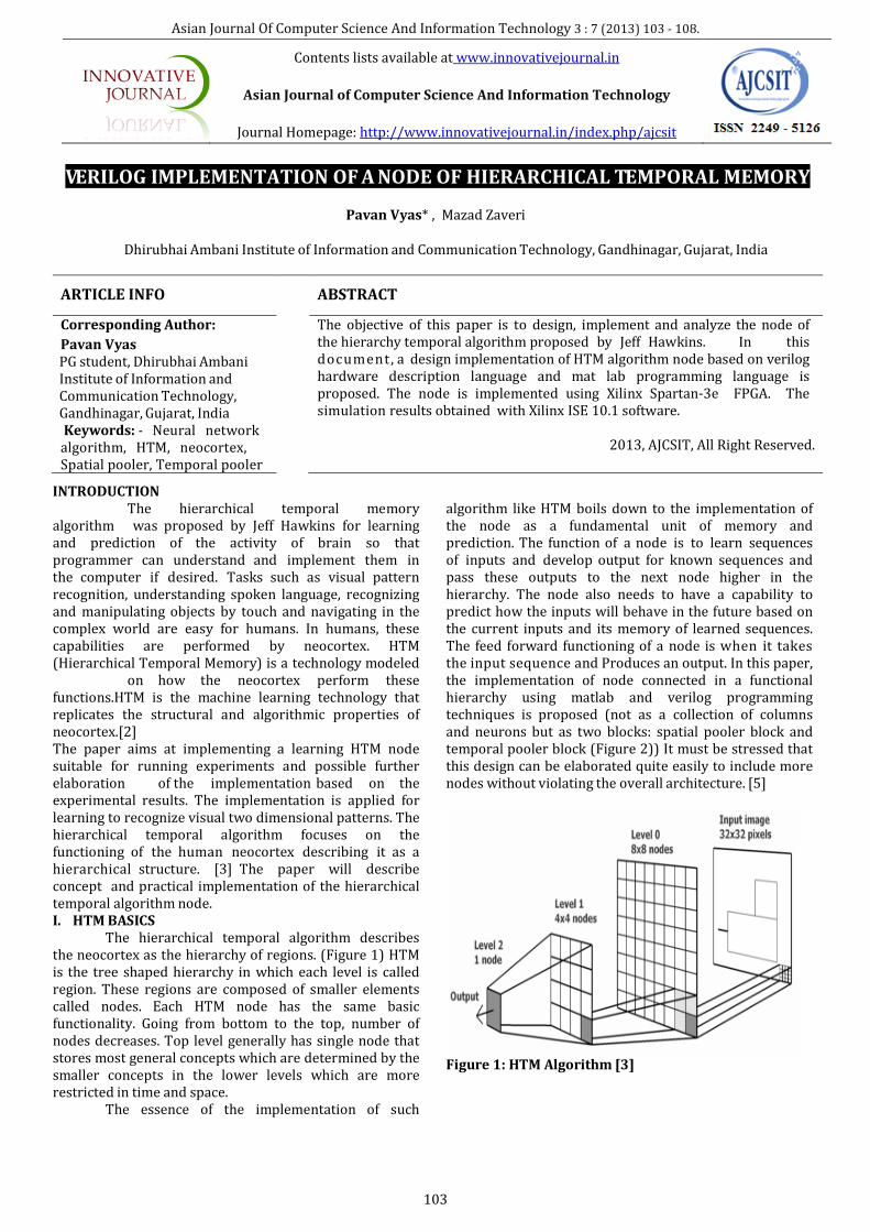
INTRODUCTION The hierarchical temporal memory algorithm was proposed by Jeff Hawkins for learning and prediction of the activity of brain so that programmer can understand and implement them in the computer if desired. Tasks such as visual pattern recognition, understanding spoken language, recognizing and manipulating objects by touch and navigating in the complex world are easy for humans. In humans, these capabilities are performed by neocortex. HTM (Hierarchical Temporal Memory) is a technology modeled on how the neocortex perform these functions.HTM is the machine learning technology that replicates the structural and algorithmic properties of neocortex.[2] The paper aims at implementing a learning HTM node suitable for running experiments and possible further elaboration of the implementation based on the experimental results. The implementation is applied for learning to recognize visual two dimensional patterns. The hierarchical temporal algorithm focuses on the functioning of the human neocortex describing it as a hierarchical structure. [3] The paper will describe concept and practical implementation of the hierarchical temporal algorithm node. I. HTM BASICS The hierarchical temporal algorithm describes the neocortex as the hierarchy of regions. (Figure 1) HTM is the tree shaped hierarchy in which each level is called region. These regions are composed of smaller elements called nodes. Each HTM node has the same basic functionality. Going from bottom to the top, number of nodes decreases. Top level generally has single node that stores most general concepts which are determined by the smaller concepts in the lower levels which are more restricted in time and space. The essence of the implementation of such

algorithm like HTM boils down to the implementation of the node as a fundamental unit of memory and prediction. The function of a node is to learn sequences of inputs and develop output for known sequences and pass these outputs to the next node higher in the hierarchy. The node also needs to have a capability to predict how the inputs will behave in the future based on the current inputs and its memory of learned sequences. The feed forward functioning of a node is when it takes the input sequence and Produces an output. In this paper, the implementation of node connected in a functional hierarchy using matlab and verilog programming techniques is proposed (not as a collection of columns and neurons but as two blocks: spatial pooler block and temporal pooler block (Figure 2)) It must be stressed that this design can be elaborated quite easily to include more nodes without violating the overall architecture. [5]

Figure 1: HTM Algorithm [3]

Vyas et.al/ Verilog Implementation of A Node Of Hierarchical Temporal Memory

104

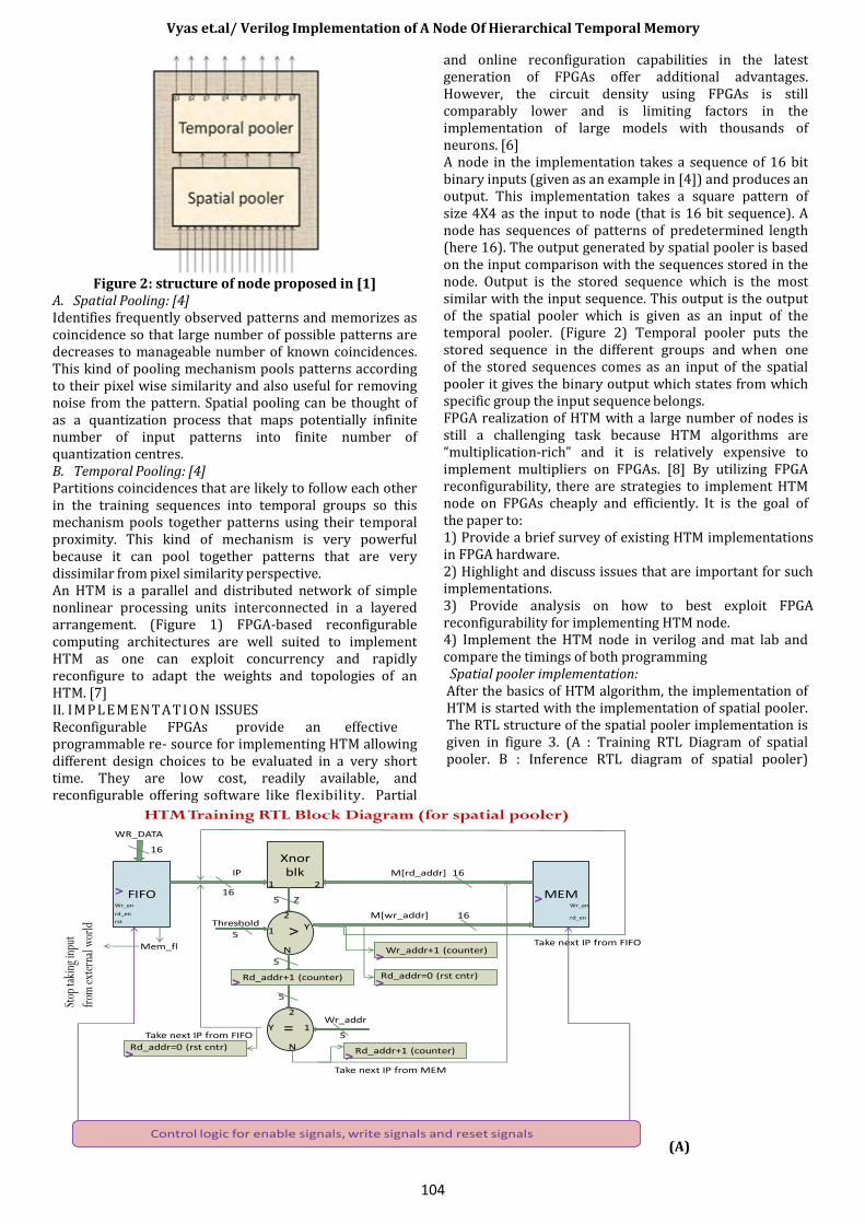
Figure 2: structure of node proposed in [1]

A. Spatial Pooling: [4] Identifies frequently observed patterns and memorizes as coincidence so that large number of possible patterns are decreases to manageable number of known coincidences. This kind of pooling mechanism pools patterns according to their pixel wise similarity and also useful for removing noise from the pattern. Spatial pooling can be thought of as a quantization process that maps potentially infinite number of input patterns into finite number of quantization centres. B. Temporal Pooling: [4] Partitions coincidences that are likely to follow each other in the training sequences into temporal groups so this mechanism pools together patterns using their temporal proximity. This kind of mechanism is very powerful because it can pool together patterns that are very dissimilar from pixel similarity perspective. An HTM is a parallel and distributed network of simple nonlinear processing units interconnected in a layered arrangement. (Figure 1) FPGA-based reconfigurable computing architectures are well suited to implement HTM as one can exploit concurrency and rapidly reconfigure to adapt the weights and topologies of an HTM. [7] II. IMPLEM E NTATION ISSUES Reconfigurable FPGAs provide an effective programmable re- source for implementing HTM allowing different design choices to be evaluated in a very short time. They are low cost, readily available, and reconfigurable offering software like flexibility. Partial

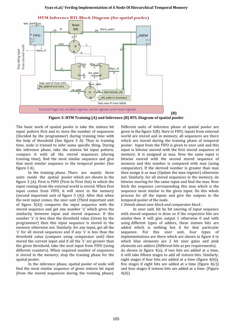
and online reconfiguration capabilities in the latest generation of FPGAs offer additional advantages. However, the circuit density using FPGAs is still comparably lower and is limiting factors in the implementation of large models with thousands of neurons. [6] A node in the implementation takes a sequence of 16 bit binary inputs (given as an example in [4]) and produces an output. This implementation takes a square pattern of size 4X4 as the input to node (that is 16 bit sequence). A node has sequences of patterns of predetermined length (here 16). The output generated by spatial pooler is based on the input comparison with the sequences stored in the node. Output is the stored sequence which is the most similar with the input sequence. This output is the output of the spatial pooler which is given as an input of the temporal pooler. (Figure 2) Temporal pooler puts the stored sequence in the different groups and when one of the stored sequences comes as an input of the spatial pooler it gives the binary output which states from which specific group the input sequence belongs. FPGA realization of HTM with a large number of nodes is still a challenging task because HTM algorithms are “multiplication-rich” and it is relatively expensive to implement multipliers on FPGAs. [8] By utilizing FPGA reconfigurability, there are strategies to implement HTM node on FPGAs cheaply and efficiently. It is the goal of the paper to: 1) Provide a brief survey of existing HTM implementations in FPGA hardware. 2) Highlight and discuss issues that are important for such implementations. 3) Provide analysis on how to best exploit FPGA reconfigurability for implementing HTM node. 4) Implement the HTM node in verilog and mat lab and compare the timings of both programming Spatial pooler implementation: After the basics of HTM algorithm, the implementation of HTM is started with the implementation of spatial pooler. The RTL structure of the spatial pooler implementation is given in figure 3. (A : Training RTL Diagram of spatial pooler. B : Inference RTL diagram of spatial pooler)

FIFO MEM

IP

WR_DATA

Mem_fl

Xnorblk M[rd_addr]

>

Z

Threshold

1 2

2

1 Y

N

M[wr_addr]

1

N

Y

2

=Wr_addr

Take next IP from FIFO

Take next IP from MEM

Rd_addr+1 (counter)

Wr_addr+1 (counter)

Rd_addr=0 (rst cntr)


Control logic for enable signals, write signals and reset signals

Rd_addr+1 (counter)

HTM Training RTL Block Diagram (for spatial pooler)

16

16

16

16

5

5

5

5

5

Stop

taki

ng in

put

from

exte

rnal

wor

ld

>>

>

>

>

>

Wr_en Wr_en

rd_enrd_en

rst

Rd_addr=0 (rst cntr)>

(A)


105

FIFO MEM

IP

WR_DATA

Mem_fl

Xnorblk M[rd_addr]

>

Z

max

1 2

2

1 Y

N


1

0

0

1

Z

max1

0

Max_rd

Rd_addr

Max_rd

Y

N

1

2

=rd_addr

wr_addr

Op=m[max_rd]



Rd_addr+1 (counter)

HTM Inference RTL Block Diagram (for spatial pooler)

16

16 16

16

5

165

5

5

5

5

5

5

5Stop

taki

ng in

put

from

ext

erna

l wor

ld

Wr_en

rd_en

rst

Wr_en

rd_en

>>

>

Rd_addr=0 (rst cntr)>

(B) Figure 3: HTM Training (A) and Inference (B) RTL Diagram of spatial pooler

The basic work of spatial pooler is take the sixteen bit input pattern first and to store the number of sequences (Decided by the programmer) during training time with the help of threshold (See figure 3 A). Thus in training time, node is trained to infer some specific thing. During the inference phase, take the sixteen bit input pattern, compare it with all the stored sequences (during training time), find the most similar sequence and give that most similar sequence to the temporal pooler (See figure 3 A). In the training phase, There are mainly three units inside the spatial pooler which are shown in the figure 3 (A). First is FIFO (First In First Out) in which the input coming from the external world is stored. When first input comes from FIFO, it will store in the memory (second important unit of figure 3 (A)). After that when the next input comes, the xnor unit (Third important unit of figure 3(A)) compares the input sequence with the stored sequence and get one number ‘z’ which gives the similarity between input and stored sequence. If this number ‘z’ is less than the threshold value (Given by the programmer) then this input sequence is stored in the memory otherwise not. Similarly, for any input, get all the ‘z’ for all stored sequences and if any ‘z’ is less than the threshold value (compare using comparator unit) then stored the current input and if all the ‘z’ zre greater than the given threshold, take the next input from FIFO (using different counters). When required number of sequences is stored in the memory, stop the training phase for the spatial pooler. In the inference phase, spatial pooler of node will find the most similar sequence of given sixteen bit input (from the stored sequences during the training phase).

Different units of inference phase of spatial pooler are given in the figure 3(B). Here in FIFO, inputs from external world are stored and in memory, all sequences are there which are stored during the training phase of temporal pooler. Input from the FIFO is given to xnor unit and this input is bitwise xnored with the first stored sequence of memory. It is assigned as max. Now the same input is bitwise xnored with the second stored sequence of memory and this number is compared with max (using comparator). If the derived number is greater than max then assign it as max (Update the max register) otherwise not. Similarly, for all stored sequences in the memory, do bitwise xnoring for the same input and find the max. Now fetch the sequence corresponding this max which is the sequence most similar to the given input. Do this whole process for all the inputs and give the outputs to the temporal pooler of the node.

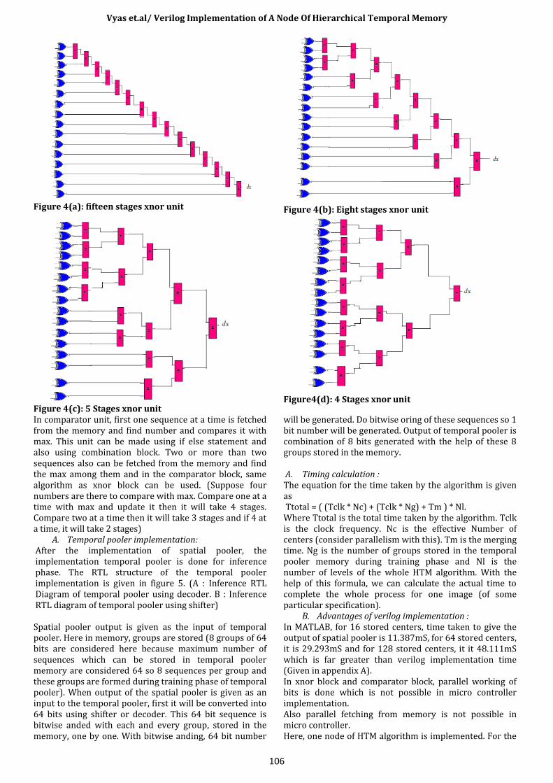
I: Details about xnor block and comparator block : In xnor unit, bit by bit xnoring of input sequence with stored sequence is done so if the respective bits are similar then it will give output 1 otherwise 0 and with using different types of adders, these sixteen bits are added which is nothing but d for that particular sequence. For this xnor unit, four types of implementations are there which are shown in figure 4 in which blue elements are 2 bit xnor gates and pink elements are adders (Different bits as per requirements). As shown in figure 4(a), if two bits are added at a time, it will take fifteen stages to add all sixteen bits. Similarly, eight stages if four bits are added at a time (figure 4(b)), five stages if eight bits are added at a time (figure 4(c)) and four stages if sixteen bits are added at a time. (Figure 4(d)).


106

Figure 4(a): fifteen stages xnor unit

Figure 4(b): Eight stages xnor unit

Figure 4(c): 5 Stages xnor unit

Figure4(d): 4 Stages xnor unit

In comparator unit, first one sequence at a time is fetched from the memory and find number and compares it with max. This unit can be made using if else statement and also using combination block. Two or more than two sequences also can be fetched from the memory and find the max among them and in the comparator block, same algorithm as xnor block can be used. (Suppose four numbers are there to compare with max. Compare one at a time with max and update it then it will take 4 stages. Compare two at a time then it will take 3 stages and if 4 at a time, it will take 2 stages)

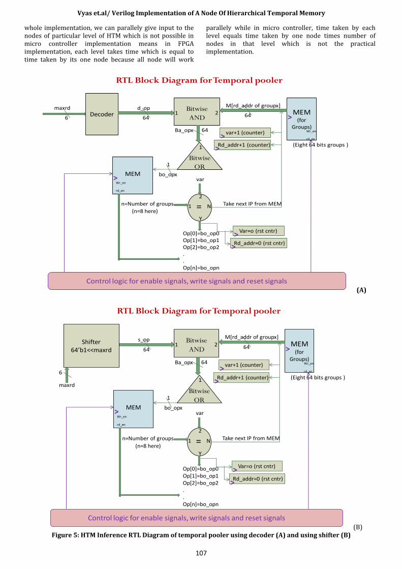
A. Temporal pooler implementation: After the implementation of spatial pooler, the implementation temporal pooler is done for inference phase. The RTL structure of the temporal pooler implementation is given in figure 5. (A : Inference RTL Diagram of temporal pooler using decoder. B : Inference RTL diagram of temporal pooler using shifter) Spatial pooler output is given as the input of temporal pooler. Here in memory, groups are stored (8 groups of 64 bits are considered here because maximum number of sequences which can be stored in temporal pooler memory are considered 64 so 8 sequences per group and these groups are formed during training phase of temporal pooler). When output of the spatial pooler is given as an input to the temporal pooler, first it will be converted into 64 bits using shifter or decoder. This 64 bit sequence is bitwise anded with each and every group, stored in the memory, one by one. With bitwise anding, 64 bit number

will be generated. Do bitwise oring of these sequences so 1 bit number will be generated. Output of temporal pooler is combination of 8 bits generated with the help of these 8 groups stored in the memory. A. Timing calculation : The equation for the time taken by the algorithm is given as Ttotal = ( (Tclk * Nc) + (Tclk * Ng) + Tm ) * Nl. Where Ttotal is the total time taken by the algorithm. Tclk is the clock frequency. Nc is the effective Number of centers (consider parallelism with this). Tm is the merging time. Ng is the number of groups stored in the temporal pooler memory during training phase and Nl is the number of levels of the whole HTM algorithm. With the help of this formula, we can calculate the actual time to complete the whole process for one image (of some particular specification).

B. Advantages of verilog implementation : In MATLAB, for 16 stored centers, time taken to give the output of spatial pooler is 11.387mS, for 64 stored centers, it is 29.293mS and for 128 stored centers, it it 48.111mS which is far greater than verilog implementation time (Given in appendix A). In xnor block and comparator block, parallel working of bits is done which is not possible in micro controller implementation. Also parallel fetching from memory is not possible in micro controller. Here, one node of HTM algorithm is implemented. For the


107

whole implementation, we can parallely give input to the nodes of particular level of HTM which is not possible in micro controller implementation means in FPGA implementation, each level takes time which is equal to time taken by its one node because all node will work

parallely while in micro controller, time taken by each level equals time taken by one node times number of nodes in that level which is not the practical implementation.

RTL Block Diagram for Temporal pooler

MEM (for

Groups)

maxrd

6Decoder

64

Bitwise

AND 64

64

Bitwise

OR

d_op

Ba_opx

M[rd_addr of groupx]

bo_opx

var+1 (counter)

Y

N1

2

=

var

n=Number of groups Take next IP from MEM

Op[0]=bo_op0Op[1]=bo_op1Op[2]=bo_op2..Op[n]=bo_opn

1

(n=8 here)

(Eight 64 bits groups )Rd_addr+1 (counter)

MEM


1 2

1

Wr_en

rd_en

Wr_en

rd_en

>

>

>

>

Var=o (rst cntr)>Rd_addr=0 (rst cntr)>

(A)

RTL Block Diagram for Temporal pooler

MEM (for

Groups)

64

Bitwise

AND 64

64

Bitwise

OR

s_op

Ba_opx

M[rd_addr of groupx]

var+1 (counter)

Y

N1

2

=

var


Op[0]=bo_op0Op[1]=bo_op1Op[2]=bo_op2..Op[n]=bo_opn

1

(Eight 64 bits groups )Rd_addr+1 (counter)

Shifter64’b1<<maxrd

6

maxrd

n=Number of groups

(n=8 here)

MEM bo_opx


Wr_en

rd_en

>

>

>

Wr_en

rd_en

>1 2

1

Var=o (rst cntr)>Rd_addr=0 (rst cntr)>

(B)Figure 5: HTM Inference RTL Diagram of temporal pooler using decoder (A) and using shifter (B)


108

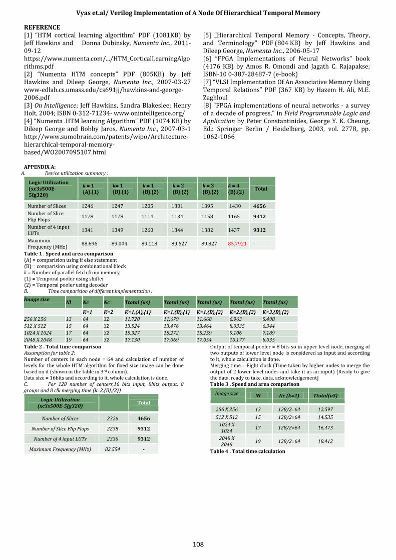
REFERENCE [1] “HTM cortical learning algorithm” PDF (1081KB) by Jeff Hawkins and Donna Dubinsky, Numenta Inc., 2011-09-12 https://www.numenta.com/.../HTM_CorticalLearningAlgorithms.pdf [2] “Numenta HTM concepts” PDF (805KB) by Jeff Hawkins and Dileep George, Numenta Inc., 2007-03-27 www-edlab.cs.umass.edu/cs691jj/hawkins-and-george-2006.pdf [3] On Intelligence; Jeff Hawkins, Sandra Blakeslee; Henry Holt, 2004; ISBN 0-312-71234- www.onintelligence.org/ [4] “Numenta .HTM learning Algorithm” PDF (1074 KB) by Dileep George and Bobby Jaros, Numenta Inc., 2007-03-1 http://www.sumobrain.com/patents/wipo/Architecture-hierarchical-temporal-memory-based/WO2007095107.html

[5] “Hierarchical Temporal Memory - Concepts, Theory, and Terminology" PDF (804 KB) by Jeff Hawkins and Dileep George, Numenta Inc., 2006-05-17 [6] “FPGA Implementations of Neural Networks” book (4176 KB) by Amos R. Omondi and Jagath C. Rajapakse; ISBN-10 0-387-28487-7 (e-book) [7] “VLSI Implementation Of An Associative Memory Using Temporal Relations” PDF (367 KB) by Hazem H. Ali, M.E. Zaghloul [8] "FPGA implementations of neural networks - a survey of a decade of progress," in Field Programmable Logic and Application by Peter Constantinides, George Y. K. Cheung, Ed.: Springer Berlin / Heidelberg, 2003, vol. 2778, pp. 1062-1066

APPENDIX A: A. Device utilization summary :

Logic Utilization (xc3s500E-5fg320)

k = 1 {A},{1}

k= 1 {B},{1}

k = 1 {B},{2}

k = 2 {B},{2}

k = 3 {B},{2}

k = 4 {B},{2}

Total

Number of Slices 1246 1247 1205 1301 1395 1430 4656

Number of Slice Flip Flops

1178 1178 1114 1134 1158 1165 9312

Number of 4 input LUTs

1341 1349 1260 1344 1382 1437 9312

Maximum Frequency (MHz)

88.696 89.004 89.118 89.627 89.827 85.7921 -

Table 1 . Speed and area comparison {A} = comparision using if else statement {B} = comparision using combinational block k = Number of parallel fetch from memory {1} = Temporal pooler using shifter {2} = Temporal pooler using decoder B. Time comparision of different implementation :

Image size Nl Nc Nc Ttotal (us) Ttotal (us) Ttotal (us) Ttotal (us) Ttotal (us)

K=1 K=2 K=1,{A},{1} K=1,{B},{1} K=1,{B},{2} K=2,{B},{2} K=3,{B},{2}

256 X 256 13 64 32 11.720 11.679 11.668 6.963 5.498

512 X 512 15 64 32 13.524 13.476 13.464 8.0335 6.344

1024 X 1024 17 64 32 15.327 15.272 15.259 9.106 7.189

2048 X 2048 19 64 32 17.130 17.069 17.054 10.177 8.035

Table 2 . Total time comparison Assumption for table 2: Number of centers in each node = 64 and calculation of number of levels for the whole HTM algorithm for fixed size image can be done based on it (shown in the table in 3rd column). Data size = 16bits and according to it, whole calculation is done.

Output of temporal pooler = 8 bits so in upper level node, merging of two outputs of lower level node is considered as input and according to it, whole calculation is done. Merging time = Eight clock (Time taken by higher nodes to merge the output of 2 lower level nodes and take it as an input) [Ready to give the data, ready to take, data, acknowledgement]

C. For 128 number of centers,16 bits input, 8bits output, 8 groups and 8 clk merging time (k=2,{B},{2})

Logic Utilization (xc3s500E-5fg320)

Total

Number of Slices 2326 4656

Number of Slice Flip Flops 2238 9312

Number of 4 input LUTs 2330 9312

Maximum Frequency (MHz) 82.554 -

Table 3 . Speed and area comparison

Image size Nl Nc (k=2) Ttotal(uS)

256 X 256 13 128/2=64 12.597

512 X 512 15 128/2=64 14.535

1024 X 1024

17 128/2=64 16.473

2048 X 2048

19 128/2=64 18.412

Table 4 . Total time calculation

verilog implementation of a node of hierarchical temporal memory

Documents