velocity of money in a modified cash-in-advance economy: theory and evidence

THEODORE PALIVOS Louisiana State University

Baton Rouge, Louisianu

PING WANG The Pennsylaania State Unitiersity

Unbersity Park, Pennsylvania

and Federal Reserve Bank of Dallas, Texas

JIANBO ZHANG Unioersity of Kansas

Lawrence, Kansas

Velocity of Money in a Modified Cash-in-Advance Economy: Theory and Evidence*

We develop a modified cash-in-advance model in which money is required prior to all the purchases of the consumption good and of a fraction of the capital good.

This framework enables us to examine the main determinants of money velocity in a dynamic general equilibrium setting. We find that, contrary to standard beliefs, high-money-growth equilibria are associated with lower welfare and lower velocity than low-money-growth equilibria. This result is supported by empirical evidence,

both over time and across countries.

1. Introduction Due to its important empirical implications, the study of money

velocity has interested economists for years. In their classic work Friedman and Schwartz (1963) attribute the movement in money velocity to factors affecting money demand as well as to the growing financial sophistication of the economy. Recently, Bordo and Jonung (1981, 1987, 1989) have extensively studied the long-run effects of institutional factors, such as financial development, on the velocity of money. Also, Rasche (1987) reconsiders the behavior of money velocity and examines whether shifts in wealth, interest rates, tax rates, trade deficits, and monetary policy variables lead to significant changes in it. However, the theoretical hypotheses identifying the movements in money velocity have not yet been completely

*We would like to thank Barry Ickes, Carol Scotese, Alan Stockman, and an anonymous referee for helpful comments. The usual disclaimer applies.

journal of Macroeconomics, Spring 1993, Vol. 15, No. 2, pp. 225-248 225 Copyright 0 1993 by Louisiana State University Press Olfx0794/93/$1.50

Theodore Palivos, Ping Wang and Jianbo Zhang

developed in the context of a general equilibrium model. In particular, most of the empirical work on money velocity relies on money demand theory in which interactions between the real and the monetary sector are omitted.

In this paper, we establish a dynamic general equilibrium model in which money is introduced through a modified cash-in-advance constraint. An unattractive characteristic of the traditional cash-in- advance models with homogeneous goods, in a deterministic setting, is that the velocity of money is independent of changes in the money growth rate. More specifically, if capital is abstracted from the cash-in-advance model (compare Lucas 1980), one obtains a un- itary velocity. By allowing for capital accumulation but assuming that money is required only for the purchases of the consumption good (compare Stockman 1981), money becomes superneutral, and hence any money growth policy will not affect money velocity. In the latter case, if money is required for the purchases of the capital good as well (compare Stockman 1981), then velocity becomes again identically one. Even within a stochastic framework (for example, see Svensson 1985), money growth may change the velocity of money, only when the cash-in-advance constraint is not binding (since in this case, long-run movements in the growth rate of money may affect real money balances and output by a different magnitude).

To allow for possible linkage between money growth and velocity in the long run, we postulate that only a fraction, 8, of the capital good is subject to the cash-in-advance constraint. This modification enables us to study the determinants of money velocity, including monetary policy, various financial institutional changes, and an output technological factor. We find that, contrary to find- ings in previous work, high-money-growth equilibria are associated with lower welfare and lower velocity than low-money-growth equilibria when this fraction (6) is given a priori. This occurs because a higher money growth rate creates an adverse effect on capital accumulation (that is, the reverse Tobin effect) and consumption. Under decreasing returns to scale, such an effect is found to sup- press money velocity. One may also allow the fraction 8 to depend on the endogenously determined inflation rate and on an exogenous factor capturing institutional changes in the financial system. In this case, if a higher money growth rate and the associated higher inflation make credit trading (of the capital good) less feasible and hence increase the fraction of the capital good subject to the cash- in-advance constraint, then there will be an additional downward pressure on the velocity of money.

226

Velocity of Money in a Modified Cash-in-Aduance Economy

Moreover, we study the long-run effects of technological improvement and financial development on macroeconomic aggregates and on the velocity of money. We show that any policy enhancing credit trading will result in higher money velocity. On the other hand, a technological improvement in production will increase both real income and real money balances, thus creating an ambiguous effect on the velocity of money. We also provide empirical evidence to lend support to our main theoretical results and find that there is a consistently negative relationship between the rate of money growth and money velocity, both over time and across countries. Finally, it should be noted that one cannot draw any conclusions from our paper to address this issue in the case of hyperinflation in which the transactions frequency is expected to change significantly over time (for details, see Section 6 below).

The remainder of the paper is organized as follows. Section 2 develops a modified cash-in-advance model, Section 3 characterizes the steady-state solution, and Section 4 demonstrates the determinants of money velocity. Empirical evidence is then provided in Section 5 and conclusions are drawn in Section 6.

2. The Model In this section, we consider a dynamic, general equilibrium

model in which money is introduced through a cash-in-advance constraint.

Preferences and Technology A representative agent with perfect foresight seeks to maxi-

mize his/her lifetime utility described by

where c is per capita consumption and l3 E (0, 1) is the constant discount rate. The felicity function, u(a), is assumed to be increasing, twice continuously differentiable, strictly concave, and to satisfy the Inada conditions, that is, u,(O) = ~0 and u,(m) = 0. In each period t, the agent produces a certain amount of output, yt, by using a common technology described by A,f(kJ, where k, denotes per capita capital stock and A, is a multiplicative technological parameter. The capital stock is assumed to be fully depreciated at the

227

Theodore Palioos, Ping Wang and Jianbo Zhang

end of each period.’ Further, the production function is assumed to be increasing, twice continuously differentiable, strictly concave, and to satisfy f(0) = 0 and the Inada conditions. In addition, at the beginning of each period the individual receives a lump sum cash transfer of amount 7, (expressed in real terms) from the govem- ment. Given any amount of income, the individual can consume it during this period, save it in the form of money, or invest it to produce in the next period.

Constraints Let P, be the price level in period t and M, be the nominal

money holdings in the beginning of period t. Next, by defining real money holdings in the beginning of period t as m, = M,/P,-,, we can write the agent’s budget constraint in real terms as:”

3 ct + mt+l + k,+, = A,f(k) + - 1 + 7r,

+ 7, >

where nt denotes the inflation rate defined as ITS = (Pt - P,-l)/P,-l. The individual is also subject to a cash-in-advance or liquidity

constraint. That is, all the purchases of the consumption good, as well as a fraction 0 of the investment good, can be made only by using money.’ The fraction (1 - 9) of the investment good, on the other hand, is purchased on credit. The same distinction between “cash” and “credit” goods can also be found in Lucas and Stokey (I987), although in the absence of capital, their credit good enters the agent’s utility function directly. It has been claimed, however, that this distinction is unlikely to be independent of the inflation rate (Blanchard and Fischer 1989). To circumvent this problem, one can allow 8 to depend on the inflation rate. In general, 8, has an ambiguous sign, since any change in the inflation rate will shift both the supply of and the demand for loanable funds. Nevertheless, if

‘For an empirical investigation of the behavior of Ml-velocity using the VAR approach see McMillin (1991).

“This assumption is made only for convenience; all the main results, derived below, remain qualitatively the same, as long as the rate of return on capital is positive; that is, Afk > 6, where 6 denotes the depreciation rate.

“The budget constraint in nominal terms is P,c, + P,k,+, + M,,, = P,A,f(k,) + M, + P,T,. By dividing both sides of this equation by P, we obtain Equation (2). It should also be noted that m,,, and k,,, measure, respectively, money and capital demands in period t while M,/P, = m,/(l + P,) denotes initial real money holdings evaluated at the end of period t.

228

Velocity of Money in a Modified Cash-in-Advance Economy

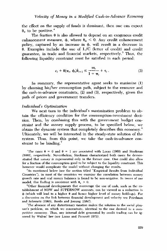
the effect on the supply of funds is dominant, then one can expect 8, to be positive.’

The fraction 8 is also allowed to depend on an exogenous credit enhancement measure, $, where 8, < 0. Any credit enhancement policy, captured by an increase in +, will result in a decrease in 8. Examples include the use of L/C (letter of credit) and credit guarantee, in trade and financial markets, respectively.” Thus, the following liquidity constraint must be satisfied in each period:

m, c, + fl(% 4)k+, 5 -

1 + 7F+ + 7, .

In summary, the representative agent seeks to maximize (1) by choosing his/her consumption path, subject to the resource and the cash-in-advance constraints, (2) and (3), respectively, given the path of prices and government transfers.

Individual’s Optimization We next turn to the individual’s maximization problem to ob-

tain the efficiency condition for the consumption-investment deci- sion. Then, by combining this with the govermnent budget constraint and the money supply process, to be specified below, we obtain the dynamic system that completely describes this economy.” Ultimately, we will be interested in the steady-state solution of the system. Thus, from this point, we take the cash-in-advance constraint to be binding.’

‘The cases 8 = 0 and 0 = 1 are associated with Lucas (1980) and Stockman (1981), respectively. Nevertheless, Stockman characterized both cases: he demon- strated that money is superneutral only in the former case. One could also allow for a fraction of the consumption good to be subject to the liquidity constraint. This

however would complicate the model without changing the results. “As mentioned below (see the section titled “Empirical Results from Individual

Countries”), in most of the countries we examine the correlation between money growth rate and real money balances is found to be non-negative. In terms of our model, this finding is consistent with 8, > 0.

60ther financial developments that encourage the use of cash, such as the es-

tablishment of NOW and SUPERNOW accounts, can be viewed as a reduction in 4 (which will lead to a higher 0 and hence higher level of money holdings). For a discussion on the link between financial development and velocity see Friedman and Schwartz (1963), Bordo and Jonung (1987).

‘The absence of any distortionary taxation makes the solution to the social plan-

ner’s problem, on which we concentrate, identical to the one derived in a com- petitive economy. Thus, any internal debt generated by credit trading can be ignored by Walras’ law (see Lucas and Prescott 1971).

Theodore Pulivos, Ping Wang and Jianbo Zhang

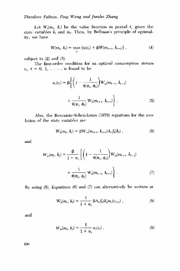
Let Wt(nz,, k,) be th e value function in period t, given the state variables k, and m,. Then, by Bellman’s principle of optimal- ity, we have

Ww k,) = lnax {ZI(CJ + PW(m,+l, k,+J) , (4) L’t

subject to (2) and (3). The first-order condition for an optimal consumption stream

c,, t = 0, 1, . . . , is found to be

(5)

Also, the Beveniste-Scheinkman (1979) equations for the evo- lution of the state variables are

Wdw, k,) = PW,,hw+,> k+,)Ath(k,) > (6)

and

(7)

By using (5), Equations (6) and (7) can alternatively be written as

and

1 W,,,(m,, k) = - f-44 .

1 + ?rt (9)

230


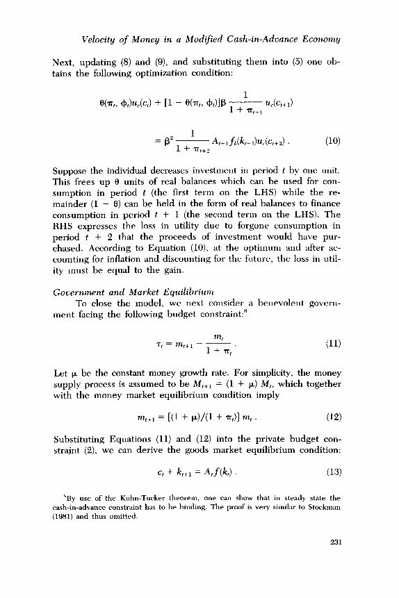
Next, updating (8) and (9), and substituting them into (5) one obtains the following optimization condition:

O(% 4M4 + [l - e(% 4)lP 1 +l, %(Ct+1) 1+1

= p” 1 +', A,+,fi(k+J~,(ct+,) . (10) t+2

Suppose the individual decreases investment in period t by one unit. This frees up CI units of real balances which can be used for consumption in period t (the first term on the LHS) while the remainder (1 - 0) can be held in the form of real balances to finance consumption in period t + 1 (the second term on the LHS). The RHS expresses the loss in utility due to forgone consumption in period t + 2 that the proceeds of investment would have purchased. According to Equation (lo), at the optimum and after ac- counting for inflation and discounting for the future, the loss in utility must be equal to the gain.

Government and Market Equilibrium To close the model, we next consider a benevolent govern-

ment facing the following budget constraint:’

Let p be the constant money growth rate. For simplicity, the money supply process is assumed to be M,,, = (1 + k) M,, which together with the money market equilibrium condition imply

m,+, = [Cl + d/O + ~11 fn, . (12)

Substituting Equations (11) and (12) into the private budget con- stramt (2), we can derive the goods market equilibrium condition:

ct + k+, = &f(k) . (13)

*By use of the Kuhn-Tucker theorem, one can show that in steady state the cash-in-advance constraint has to be binding. The proof is very similar to Stockman (1981) and thus omitted.

231


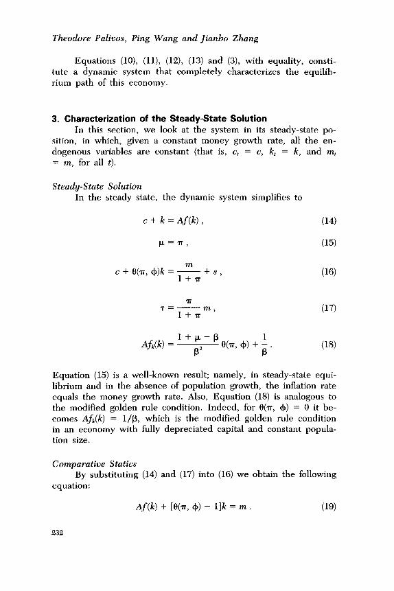
Equations (lo), (ll), (12), (13) and (3), with equality, consti- tute a dynamic system that completely characterizes the equilibrium path of this economy.

3. Characterization of the Steady-State Solution In this section, we look at the system in its steady-state po-

sition, in which, given a constant money growth rate, all the en- dogenous variables are constant (that is, cf = c, k, = k, and m, = m, for all t).

Steady-State Solution In the steady state, the dynamic system simplifies to

c + k = Af(k) , (14)

p=n, (15)

c + e(m, +)k = m + s , 1+7F

06)

7F T=l+mm’

AfLk) = l+F-P

P”

(17)

Equation (15) is a well-known result; namely, in steady-state equilibrium and in the absence of population growth, the inflation rate equals the money growth rate. Also, Equation (18) is analogous to the modified golden rule condition. Indeed, for O(T, +) = 0 it becomes Afk(k) = l/B, which is the modified golden rule condition in an economy with fully depreciated capital and constant population size.

Comparative Statics By substituting (14) and (17) into (16) we obtain the following

equation:

Af(k) + [e(n, 4) - l]k = m . (1%

2.32


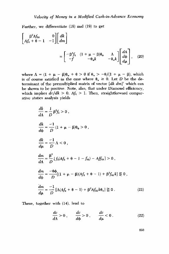
Further, we differentiate (18) and (19) to get

P Wikk 0 dk Af,+O-1 -1 I[ 1 dm

r -P% (1 + P - w, A = -f -8,k -jJ

where A = (1 + t.~ - p)t$, + 0 > 0 if 0, > -O/(1 + t.~ - p), which is of course satisfied in the case where 8, 2 0. Let D be the de- terminant of the premultiplied matrix of vector [dk dm]’ which can be shown to be positive. Note, also, that under Diamond effkiency, which implies dc/dk > 0, Afk > 1. Then, straightforward comparative statics analysis yields

dk -1 - - (1 + /J, - p)e, > 0,

G-D

dk -1 -=- 6 D

A-CO,

dm p” ~=D[~(Af~+e-l-~~)-Affkkl>O,

dm - ?[(l + t.r, - p)(Afk + 0 - 1) + Pykfkkk] $ 0,

z- D

dm -1 -= &

D [A(Afk + 8 - 1) + P2Afkkk0,] $0 .

These, together with (14), lead to

dc dc dc ->o, -co. dA

->o, d+ &

(21)

(22)

233


Intuitively, a technological improvement increases the marginal product of capital and thus increases the steady-state level of capital. Under Diamond efficiency, consumption will increase as well. Hence, to finance a higher level of consumption and investment, real money balances must also increase.

Any financial improvement which decreases 8, and is captured by an increase in +, has a direct negative effect on real money holdings and results in a lower marginal cost of capital. This leads to higher levels of consumption and capital, which in turn require more money to facilitate transactions. Overall, the net effect on money holdings is ambiguous.

Finally, money is not superneutral. More specifically, higher rates of money growth are likely associated with lower steady-state levels of capital (that is, reverse Tobin effect) and consumption, thus decreasing social welfare.’ It is important to distinguish again between the two different effects that may lead to this result. A higher rate of money growth implies a higher rate of inflation. Even with an exogenous 0 (that is, 8, = 0), an increase in inflation will raise the cost of money holdings and thus it will decrease the net rate of return on capital. This will cause in turn a decrease in investment and consumption. However, 8 can be allowed to depend on the endogenously determined inflation rate. In the case of 8, > 0 an increase in inflation will also increase 0, which is equivalent to an increase in the shadow cost of capital. Thus, the level of investment and hence consumption will fall even more. This reverse Tobin effect can be obtained even if 8, < 0. A sufficient condition for this is: 8, > -O/(1 + u, - p). If, however, an increase in inflation causes a sufficient increase in the fraction of the investment good purchased on credit, then the shadow cost of capital will decrease. In this case the Tobin effect (see Tobin 1965) will be present contrary to the standard cash-in-advance models. Finally, as in the case of a change in +, the effect of money growth expansion on the level of real money balances is ambiguous.”

4. Velocity of Money This section examines the determinants of the income velocity

of money and elaborates on related issues. Specifically, we study

‘In nominal terms, this constraint is P,T, = M,,, - M,. “‘These should be viewed as anticipated changes in the money growth rate, sim-

ilar to Brock (1975).

234


how money velocity is affected by changes in the exogenous variables: A, $, and F.

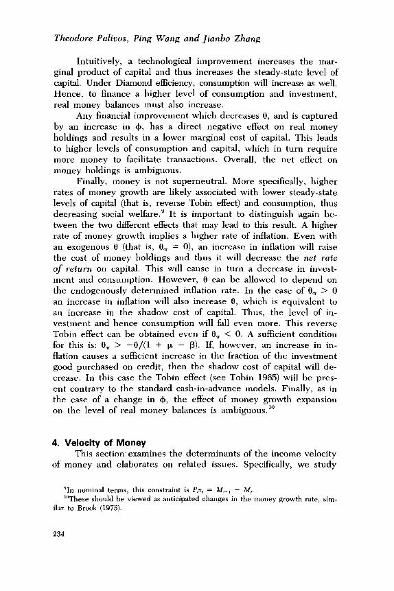
Determinants of Money Velocity In terms of the theoretical model, the velocity of money is

defined as

c+k c+k V=-=- m c + Ok ’

(23)

Thus higher 8, ceteris paribus, decreases money velocity. By totally differentiating (23) and using (21) one obtains the

additional comparative statics results:”

dV dV ----SO dvz 0. dA

->o, ’ d+ dk

=z (24)

As mentioned in Section 3, an improvement in the technological parameter (A) will increase the steady-state levels of capital, consumption, and real money balances. Hence, the effect on velocity is indeterminate.

Any credit enhancement policy, captured by an increase in 4, will create a direct downward effect on 8 and thus it will increase velocity through the reduction of money holdings. It will also increase consumption and capital accumulation, as indicated in (21) and (22), which will in turn lead to a further increase of money velocity, under the presumption of 0 < 1. Therefore, money velocity will unambiguously increase.

Finally, the velocity of money may depend negatively on the money growth rate and thus it may be inversely related to the inflation rate. Notice that in a traditional monetary model, an increase

“We have performed a calibration exercise to study this issue using the func- tional forms f(k) = k” and 6(n, $) = t3(n, 1) = [(n/l + n)]” and the following parameter values: (I = 0.28 (the average labor income share in the U.S. computed from NIPA accounts), l3 = 0.988 and r = 6.5% (both taken from King et al. 1988), b = 0.15 (computed from Equation [IS], using p = 6.54%, which is the average value in the U.S. over the period 1963-1985). and A”‘-“’ = 1.65 (calculated in such a way that the output level corresponding to p. = 0 is normalized to one). We have found that, as IL rises, real balances initially increase due to the direct effect of 8, reach a peak at approximately p = ll%, and eventually decrease because of the high opportunity cost of holding money.

235


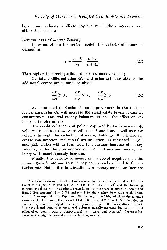
in the rate of inflation increases the cost of money holdings, and thus money demand falls relative to output. Our cash-in-advance model takes this reasoning one step further, since it emphasizes also the transactions demand for money (people need cash to finance real purchases of consumption and capital good). To acquire a better understanding of the negative relationship between money growth rate and money velocity we manipulate (23) to obtain

1 v=

1 - (1 - @k/y ’

where y = c + k. By differentiating (25) we have

where d(k/y)/dp = [(f - kfk)/Af’] (dk/dp) < 0, under the assumption of decreasing returns to scale in the per capita output production function, that is, f - kfk > 0.

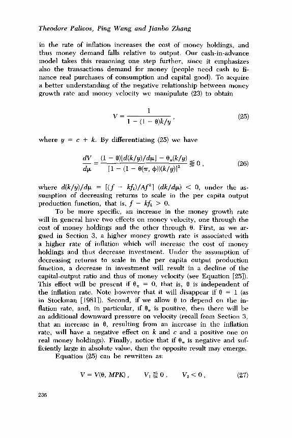
To be more specific, an increase in the money growth rate will in general have two effects on money velocity, one through the cost of money holdings and the other through 8. First, as we ar- gued in Section 3, a higher money growth rate is associated with a higher rate of inflation which will increase the cost of money holdings and thus decrease investment. Under the assumption of decreasing returns to scale in the per capita output production function, a decrease in investment will result in a decline of the capital-output ratio and thus of money velocity (see Equation [25]). This effect will be present if 8, = 0, that is, 8 is independent of the inflation rate. Note however that it will disappear if 0 = 1 (as in Stockman [1981]). Second, if we allow 8 to depend on the inflation rate, and, in particular, if 8, is positive, then there will be an additional downward pressure on velocity (recall from Section 3, that an increase in 8, resulting from an increase in the inflation rate, will have a negative effect on k and c and a positive one on real money holdings). Finally, notice that if 8, is negative and suf- ficiently large in absolute value, then the opposite result may emerge.

Equation (25) can be rewritten as:

v = v(e, MPK) ) v120, v,<o, (27)

236


where MPK, the marginal product of capital, is negatively corre- lated with the capital-output ratio. Thus, all the effects mentioned above can be decomposed into effects through 0 and through MPK. By using (Zl), one can obtain the following reduced form equation:

V = g(p> 4 A) , (28)

where g, $ 0, g, > 0 and g, $ 0 .

Further Discussion Traditionally, based on Baumol (1952), and Tobin (1956), the

velocity of money is expressed as a function of real income and nominal interest rate (i). That is,

V = h( y, i)

where

h,>o, h,>O,

V=h(y,r+$, (2%

where r is the real interest rate and is analogous to MPK in (27). Nevertheless, (29) is derived within a partial equilibrium framework in which both y and r are not endogenized. In fact, this is exactly the point that we try to emphasize in this section, that is, that ceteris will not remain paribus and that both y and r in Equation (29) will change as TV and thus 7~ change.

5. Empirical Evidence In this section, we examine more closely the inverse relation-

ship between velocity and money growth rate and draw some evidence from the U.S. and several other countries as well.

The Data We choose a group of twenty representative countries for our

econometric analysis. The selection of countries is based upon the following criteria:

237


(i) the availability of data during the sample period, 1963- 1985; (ii) the quality of the data (see Summers and Heston 1988);

(iii) co-movements between money growth and inflation rates, in order to satisfy the equality p = n (implied by our theoretical model), a necessary condition for a country to be on a long-run equilibrium path. l2 The satisfaction of this criterion is based on the data provided in Barro (1990, Table 7.1);13 and (iv) the comprehensiveness of the data reflecting the charac-

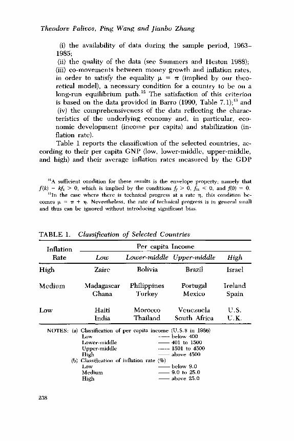
teristics of the underlying economy and, in particular, economic development (income per capita) and stabilization (inflation rate). Table 1 reports the classification of the selected countries, ac-

cording to their per capita GNP (low, lower-middle, upper-middle, and high) and their average inflation rates measured by the GDP

“A sufficient condition for these results is the envelope property; namely that f(k) - Icfk > 0, which is implied by the conditions f, > 0, fik < 0, and f(O) = 0.

l3In the case where there is technical progress at a rate q, this condition becomes p = n + n. Nevertheless, the rate of technical progress is in general small and thus can be ignored without introducing significant bias.

TABLE 1. Classification of Selected Countries

Inflation Rate LOW

Per capita Income

Lower-middle Upper-middle High

High Zaire Bolivia Brazil Israel

Medium Madagascar Philippines Portugal Ireland Ghana Turkey Mexico Spain

Low Haiti India

Morocco Thailand

Venezuela U. S. South Africa U.K.

NOTES: (a) Classification of per capita income (U.S.0 in 1986) Low - below 400 Lower-middle - 401 to 1500 Upper-middle - 1501 to 4500 High ~ above 4500

(b) Classification of inflation rate (%) Low ~ below 9.0 Medium - 9.0 to 25.0 High - above 25.0

238


deflator (low, middle, and high).‘” Geographically, this sample includes 6 countries from America (Bolivia, Brazil, Haiti, Mexico, Venezuela, and the U.S.), 5 from Africa (Zaire, Madagascar, Ghana, Morocco, and South Africa), 5 from Europe (Turkey, Portugal, Ire- land, Spain, and the U.K.), and 4 from Asia (India, Philippines, Thailand, and Israel). Their values of per capita GNP range from 160 U.S.$ in 1986 (Haiti) to 17,480 (U.S.), while their annual inflation rates fall between 5.38% (Thailand) and 55.92% (Bolivia).

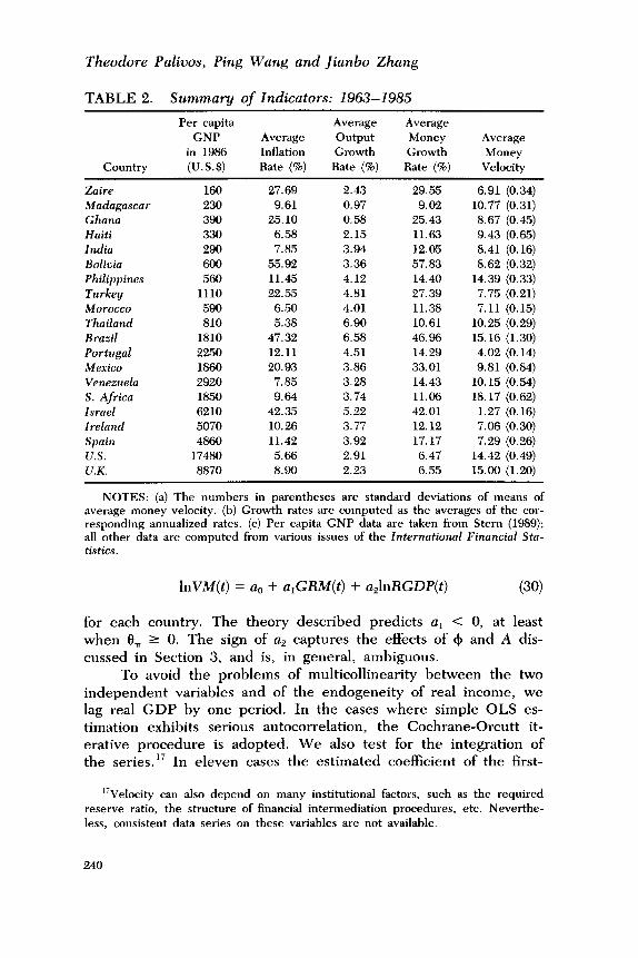
The output measure is real GDP and the money supply measure is the monetary base. Money velocity is therefore defined as the ratio of nominal GDP to monetary base. I5

Since the money growth rate in our theoretical framework is exogenous to the individual’s optimization problem, we use the monetary base in lieu of Ml. Nevertheless, by comparing different measures of money supply (currency, monetary base, and Ml), we find that movements in the associated velocity measure are gen- erally similar. For the twenty selected countries, the average money growth rates range between 6.47% (U.S.) and 57.83% (Bolivia), and the average money velocity measures fall in between 1.27 (Israel) and 18.17 (South Africa). Among all the countries, Brazil has the most volatile money velocity (the standard deviation of the mean is 1.30), while Portugal’s money velocity is the smoothest (the standard deviation of the mean is 0.14)-see Table 2 for a summary of main indicators.

Empirical Results from Individual Countries We next perform a time-series analysis for each individual

country. In the absence of precise measures of financial and economic development, we incorporate real GDP (RGDP) into the regression of money velocity (VM), as well as the key variable- the rate of money growth (GRM).lfi The regression is specified as

“Except for a few cases where we have no alternative, we restrict z = (p - P)/[(P + ~r)/2] to be less than 0.3.

ISThe high-inflation category includes only four counties, either because these countries are unique (Zaire, Israel) or because the data series for other high-inflation countries are not available for the entire period 1963-1984. Moreover, ctite-

rion (iii) excludes all other countries (except U.S., U.K. and France) in the G7 group, since z is far from zero (for example, for West Germany and Japan, it is 0.75 and 0.78, respectively.) The results for France are reported in footnote 20

below. ‘“For a comprehensive discussion on various types of velocity, that is, income,

transaction, and financial, using Ml and the monetary base, see Osborne (1986).

239


TABLE 2. Summary of Indicators: 1963-1985

Per capita Average Average GNP Average output Money Average

in 1986 Inflation Growth Growth Money Country (U.S.$) Rate (%) Rate (%) Rate (%) Velocity

Zaire 160 27.69 Madagascar 230 9.61 Ghana 390 25.10 Haiti 330 6.58 India 290 7.85 Bolinia 600 55.92 Philippines 560 11.45 Turkey 1110 22.55 Morocco 590 6.50 Thailand 810 5.38 Brazil 1810 47.32 Portugal 2250 12.11 Mexico 1860 20.93 Venezuela 2920 7.85 S. Aftica 1850 9.64 Israel 6210 42.35 Irelund 5070 10.26 Spain 4860 11.42 U.S. 17480 5.66 U.K. 8870 8.90

2.43 29.55 6.91 (0.34) 0.97 9.02 10.77 (0.31) 0.58 25.43 8.67 (0.45) 2.15 11.63 9.43 (0.65) 3.94 12.05 8.41 (0.16) 3.36 57.83 8.62 (0.32) 4.12 14.40 14.39 (0.33) 4.81 27.39 7.75 (0.21) 4.01 11.38 7.11 (0.15) 6.90 10.61 10.25 (0.29) 6.58 46.96 15.16 (1.30) 4.51 14.29 4.02 (0.14) 3.86 33.01 9.81 (0.84) 3.28 14.43 10.15 (0.54) 3.74 11.06 18.17 (0.62) 5.22 42.01 1.27 (0.16) 3.77 12.12 7.06 (0.30) 3.92 17.17 7.29 (0.26) 2.91 6.47 14.42 (0.49) 2.23 6.55 15.00 (1.20)

NOTES: (a) The numbers in parentheses are standard deviations of means of average money velocity. (b) G rowth rates are computed as the averages of the corresponding annualized rates. (c) Per capita GNP data are taken from Stern (1989); all other data are computed from various issues of the Znternational Financial Sta- tistics.

lnVM(t) = a,, + a,GRM(t) + a,lnRGDP(t)

for each country. The theory described predicts a, < 0, at least when 8, 2 0. The sign of a2 captures the effects of + and A dis- cussed in Section 3, and is, in general, ambiguous.

To avoid the problems of multicollinearity between the two independent variables and of the endogeneity of real income, we lag real GDP by one period. In the cases where simple OLS estimation exhibits serious autocorrelation, the Cochrane-Orcutt it- erative procedure is adopted. We also test for the integration of the series.” In eleven cases the estimated coefficient of the first-

“Velocity can also depend on many institutional factors, such as the required reserve ratio, the structure of financial intermediation procedures, etc. Neverthe- less. consistent data series on these variables are not available.

240


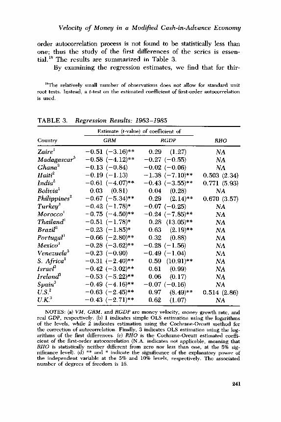
order autocorrelation process is not found to be statistically less than one; thus the study of the first differences of the series is essential. lx The results are summarized in Table 3.

By examining the regression estimates, we find that for thir-

‘*The relatively small number of observations does not allow for standard unit

root tests. Instead, a t-test on the estimated coefficient of first-order autocorrelation is used.

TABLE 3. Regression Results: 1963-l 98.5

Country

Estimate (t-value) of coeffkient of

GRM RGDP RHO

Zaire’ -0.51 (-3.16)** Madagascar3 -0.58 (-4.12)** Ghana3 -0.13 (-0.84) Haiti” -0.19 (-1.13) India” -0.61 (-4.07)** Bolivia’ 0.03 (0.81) Philippines” -0.67 (-5.34)** Turkey3 -0.42 (-1.78)* Morocco’ -0.75 (-4.50)** Thailand’ -0.51 (-1.78)* Brazil3 -0.23 (-1.85)* Portugar -0.66 (-2.80)** Mexico3 -0.28 (-3.62)** Venezuela3 -0.23 (-0.90) S. Africa’ -0.31 (-2.40)** Israe? -0.42 (-3.02)** Irelandj -0.53 (-5.22)** Spain3 -0.49 (-4.16)** U.S.2 -0.63 (-2.45)** U.K.3 -0.43 (-2.71)**

0.29 (1.27) -0.27 (-0.55) -0.02 (-0.06) -1.38 (-7.10)** -0.43 (-3.55)**

0.04 (0.28) 0.29 (2.14)**

-0.07 (-0.25) -0.24 (-7.85)**

0.28 (13.05)** 0.63 (2.19)** 0.32 (0.88)

-0.28 (-1.56) -0.49 (-1.04)

0.59 (10.91)** 0.61 (0.99) 0.06 (0.17)

-0.07 (-0.16) 0.97 (8.49)** 0.62 (1.07)

NA NA NA

0.503 (2.34) 0.771 (5.93)

NA 0.670 (3.57)

NA NA NA NA NA NA NA NA NA NA NA

0.514 (2.86) NA

NOTES: (a) VM, GRM, and RGDP are money velocity, money growth rate, and real GDP, respectively. (b) 1 indicates simple OLS estimation using the logarithms of the levels, while 2 indicates estimation using the Cochrane-Orcutt method for the correction of autocorrelation. Finally, 3 indicates OLS estimation using the logarithms of the first differences. (c) RHO is the Cochrane-Orcutt estimated coefficient of the first-order autocorrelation (N.A. indicates not applicable, meaning that RHO is statistically neither different from zero nor less than one, at the 5% significance level). (d) ** and * indicate the significance of the explanatory power of the independent variable at the 5% and 10% levels, respectively. The associated number of degrees of freedom is 16.

241


teen (sixteen) out of twenty countries the effects of money growth on money velocity are significantly negative at the 5% (10%) level.” The effects of real income, on the other hand, are not so significant, especially after correcting the autocorrelation problem. This could be the case because of the following reasons: (i) as we showed in Section 4, an increase in the technological parameter, A, will have two offsetting effects on money velocity; and, (ii) the level of GDP may capture both credit enhancement policies and financial development programs that encourage the use of money. We have also examined the correlation between real money balances and the money growth rate. In most cases, we have found the correlation coefficient to be non-negative, which, in terms of our model, is consistent with 8, > 0.

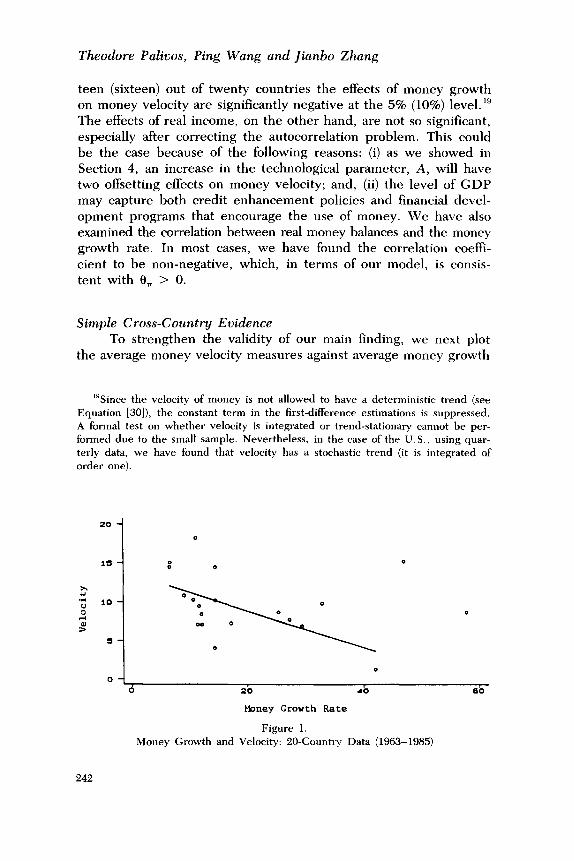
Simple Cross-Country Evidence To strengthen the validity of our main finding, we next plot

the average money velocity measures against average money growth

‘“Since the velocity of money is not allowed to have a deterministic trend (see Equation [30]), the constant term in the first-difference estimations is suppressed. A formal test on whether velocity is integrated or trend-stationary cannot be performed due to the small sample. Nevertheless, in the case of the U.S., using quarterly data, we have found that velocity has a stochastic trend (it is integrated of order one).

0 0

d 20 *o 60

Maney Growth Rate

Figure 1. Money Growth and Velocity: 20-Country Data (1963-1985)

242


rate for all countries, as shown in Figure 1.“” Excluding Bolivia and Brazil, which are the two countries with the highest inflation rate in the sample, one can see the negative relation between the two variables. That is, for countries with higher money growth, their velocities of money tend to be lower. The overall correlation coefficient is -0.26, but if we exclude Bolivia and Brazil from the sample it becomes -0.58. The same result obtains even if we replace the money growth rate by the inflation rate (the correlation coefficient is -0.21 and if we exclude Bolivia and Brazil it becomes -0.55).

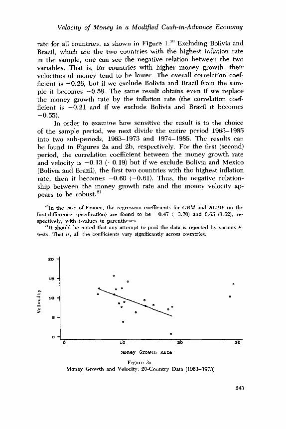
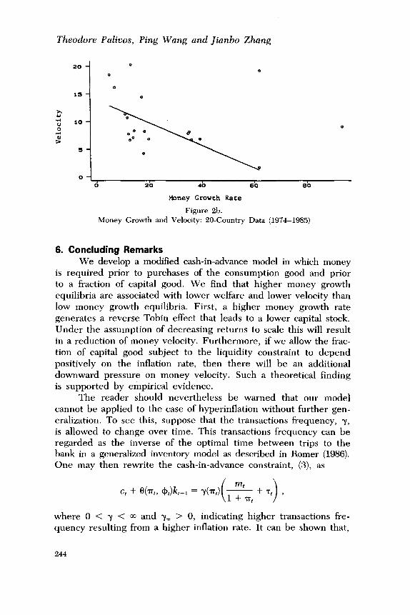
In order to examine how sensitive the result is to the choice of the sample period, we next divide the entire period 1963-1985 into two sub-periods, 1963-1973 and 1974-1985. The results can be found in Figures 2a and 2b, respectively. For the first (second) period, the correlation coefficient between the money growth rate and velocity is -0.13 (-0.19) b u i we exclude Bolivia and Mexico t f (Bolivia and Brazil), the first two countries with the highest inflation rate, then it becomes -0.60 (-0.61). Thus, the negative relationship between the money growth rate and the money velocity ap- pears to be robust.“’

% the case of France, the regression coefficients for GRM and RGDP (in the first-difference specification) are found to be -0.47 (-3.70) and 0.65 (1.62), respectively, with t-values in parentheses.

“‘It should be noted that any attempt to pool the data is rejected by various F- tests. That is, all the coeffkients vary significantly across countries.

.Xoney Growth Rate

Figure 2a. Money Growth and Velocity: 20-Country Data (1963-1973)

243

Theodore Paliuos, Ping Wang and Jianbo Zhang

Xoney Growth Rate

Figure 2b. Money Growth and Velocity: 20-Country Data (1974-1985)

6. Concluding Remarks We develop a modified cash-in-advance model in which money

is required prior to purchases of the consumption good and prior to a fraction of capital good. We find that higher money growth equilibria are associated with lower welfare and lower velocity than low money growth equilibria. First, a higher money growth rate generates a reverse Tobin effect that leads to a lower capital stock. Under the assumption of decreasing returns to scale this will result in a reduction of money velocity. Furthermore, if we allow the fraction of capital good subject to the liquidity constraint to depend positively on the inflation rate, then there will be an additional downward pressure on money velocity. Such a theoretical finding is supported by empirical evidence.

The reader should nevertheless be warned that our model cannot be applied to the case of hyperinflation without further gen- eralization. To see this, suppose that the transactions frequency, y, is allowed to change over time. This transactions frequency can be regarded as the inverse of the optimal time between trips to the bank in a generalized inventory model as described in Romer (1986). One may then rewrite the cash-in-advance constraint, (S), as

where 0 < y < 03 and y= > 0, indicating higher transactions frequency resulting from a higher inflation rate. It can be shown that,

244


with this modification, the effect of a higher money growth rate on the velocity of money becomes ambiguous. Note however that the countries we selected for our empirical study have not reached the stage of hyperinflation and hence the transactions frequency effect is not expected to be very influential.“”

In this paper we have assumed the presence of decreasing returns to scale with respect to per capita capital. Recently, there has been an interest in models of constant (Rebel0 1991) or increasing returns to scale (Romer 1986). In these models changes in the money growth rate will aflect not only the level but also the growth rate of output. We believe that it would be interesting to use the framework developed here and examine the effects of money growth on velocity in the presence of a non-decreasing returns to scale technology. We leave this, however, as a topic for future re- search.

Received: Febnrary 1991 Final version: June 1992

References Barro, Robert J. Macroeconomics. 3d ed. New York: John Wiley &

Sons, 1990. Baumol, William J. “The Transactions Demand for Cash: An In-

ventory Theoretic Approach.” Quarterly Journal of Economics 67 (November 1952): 545-56.

Beveniste, Lawrence M., and Jose Scheinkman. “On the Differ- entiability of the Value Function in Dynamic Models of Econom- ics.” Econometrica 47 (May 1979): 727-32.

Blanchard, Olivier J., and Stanley Fischer. Lectures on Macroeco- nomics. Cambridge, MA: The MIT Press, 1989.

Bordo, Michael D., and Lars Jonung. “The Long-Run Behavior of the Income Velocity of Money: A Cross Country Comparison of Five Advanced Countries, 1870-1975.” Economic Inquiry 19 (January 1981): 96-116.

=One might tend to think that there is a bias introduced by our selection criteria. This could be the case if technical progress, population growth, and/or the transactions frequency play an essential role. Nevertheless, we believe that by se- lecting countries from different income and inflation groups the effect of such a possible bias has been minimized.

245


-. The Long-Run Behavior of the Velocity of Circulation: The international Evidence. New York: Cambridge University Press, 1987.

-. “The Long-Run Behavior of Velocity: The Institutional Ap- proach Revisited.” Journal of Policy Modeling 12 (Summer 1990): 165-97.

Brock, William A. “A Simple Perfect Foresight Monetary Model.” Journal of Monetary Economics 1 (April 1975): 133-50.

Friedman, Milton, and Anna J. Schwartz. A Monetary History of the United States, 1867-1960. Princeton, New Jersey: Princeton University Press, 1963.

King, Robert G., Charles I. Plosser, and Sergio T. Rebelo. “Pro- duction, Growth and Business Cycles: I. The Basic Neoclassical Model.” Journal of Monetary Economics 21 (March/May 1988): 195-232.

Lucas, Robert E., Jr. “Equilibrium in a Pure Currency Economy.” Economic Inquiry 18 (April 1980): 203-20.

Lucas, Robert E., Jr., and Edward C. Prescott. “Investment under Uncertainty.” Econometrica 39 (September 1971): 659-81.

Lucas, Robert E., Jr., and Nancy L. Stokey. “Money and Interest in a Cash-in-Advance Economy.” Econometrica 55 (May 1987): 491-514.

McMillin, W. Douglas. “The Velocity of Ml in the 1980s: Evidence from a Multivariate Times Series Model.” Southern Economic Journal 57 (January 1991): 634-48.

Osborne, Dale K. “Velocities of Ml and the Monetary Base: A Cor- rection of Standard Formulas.” The Federal Reserve Bank of Dallas Economic Review (January 1986): 10-24.

Rasche, Robert H. “M-l Velocity and Money Demand Functions: Do Stable Relationships Exist ?” Carnegie-Rochester Conference Series on Public Policy, no. 27 (Autumn 1987): 9-88.

Rebelo, Sergio. “Long-Run Policy Analysis and Long-Run Growth.” Journal of Political Economy 99 (June 1991): 500-21.

Romer, David. “A Simple General Equilibrium Version of the Bau- mol-Tobin Model.” Quarterly Journal of Economics 101 (Novem- ber 1986): 663-85.

Romer, Paul M. “Increasing Returns and Long-Run Growth.” Jour- nal of Politica Economy 94 (October 1986): 1002-37.

Stern, Nicholas. “The Economics of Development: A Survey.” Eco- nomic Journal 99 (September 1989): 597-685.

Stockman, Alan C. “Anticipated Inflation and the Capital Stock in

246


a Cash-in-Advance Economy.” Journal of Monetary Economics 8 (November 1981): 387-93.

Summers, Robert, and Alan Heston. “A New Set of International Comparisons of Real Product and Price Levels Estimates for 130 Countries, 1950-1985.” Review of Income and Wealth 34 (March 1988): l-25.

Svensson, Lars E.O. “Money and Asset Prices in a Cash-in-Ad- vance Economy.” Journal of Political Economy 93 (October 1985): 919-44.

Tobin, James. “The Interest-Elasticity of the Transactions Demand for Cash.” Review of Economics and Statistics 38 (September 1956): 241-47.

“Money and 1965): 671-84.

Economic Growth.” Econometrica 33 (October

Appendix

List of Symbols

A = Technological parameter. c = Per capita consumption. f = Production function. i = Nominal interest rate. k = Per capita capital.

M = Nominal money holdings in the beginning of a period. m = Real money holdings in the beginning of a period. P = Price level. r = Real interest rate. t = Time index.

U = Lifetime utility function. u = Felicity function. V = Velocity of money.

W = Value function. Y = Per capita output.

GRM = Growth rate of the monetary base. MPK = Marginal product of capital.

RGDP = Real GDP. VM = Money velocity measured as nominal GDP/monetary

base.

247


p = Discount rate. y = Transactions frequency. 8 = Fraction of the capital good subject to C-I-A constraint, p. = Money growth rate. 7~ = Inflation rate. 7 = Lump sum cash transfer. 4 = Parameter measuring credit enhancement. Zj = Partial derivative of I with respect to its jth argument,

248

velocity of money in a modified cash-in-advance economy: theory and evidence

Documents