lable at ScienceDirect

Journal of South American Earth Sciences 31 (2011) 214e226

Contents lists avai

Journal of South American Earth Sciences

journal homepage: www.elsevier .com/locate/ jsames

Variability of atmospheric precipitable water in northern Chile: Impactson interpretation of InSAR data for earthquake modeling

D. Remya,*, M. Falvey b, S. Bonvalot a, M. Chlieh c, G. Gabalda a, J.-L. Froger d, D. Legrand b

aGET (UMR CNRS/IRD/UT3 UMR5563 UR234) Obs. Midi Pyrénée, 14 av. E. Belin, 31400 Toulouse, FrancebDepartamento de Geofisica, Facultad de Ciencias Físicas y Matemáticas, Universidad de Chile e Blanco Encalada 2002, Santiago, Chilec Institut de Recherche pour le Développement (IRD), GeoAzur (Université de Nice-CNRS-IRD-OCA), Bât 4, 250 rue Albert Einstein, Sophia Antipolis, 06560 Valbonne, Franced LMV (UBP-CNRS-IRD), Obs. de Physique du Globe de Clermont-Ferrand, 5 rue Kessler, 63038 Clermont-Ferrand Cedex, France

a r t i c l e i n f o

Article history:Received 22 February 2010Accepted 17 January 2011

Keywords:InterferometryEarthquake modelingDeformationTroposphereNorthern Chile

* Corresponding author. Tel.: þ33 (0)5 61 33 26 69E-mail address: remy@lmtg.obs-mip.fr (D. Remy).

0895-9811/$ e see front matter � 2011 Elsevier Ltd.doi:10.1016/j.jsames.2011.01.003

a b s t r a c t

The use of Synthetic Aperture Radar interferometry (InSAR) in northern Chile, one of the most seismicallyactive regions in theworld, is of great importance. InSAR enables geodesists not only to accuratelymeasureEarth’s motions but also to improve fault slip map resolution and our knowledge of the time evolution ofthe earthquake cycle processes. Fault slipmapping is critical to better understand themechanical behaviorof seismogenic zones and has fundamental implications for assessing hazards associated with megathrustearthquakes. However, numerous sources of errors can significantly affect the accuracy of the geophysicalparameters deduced by InSAR. Among them, atmospheric phase delays caused by changes in the distri-bution of water vapor can lead to biased model parameter estimates and/or to difficulties in interpretingdeformation events captured with InSAR. The hyper-arid climate of northern Chile might suggest thatdifferential delays are of a minor importance for the application of InSAR techniques. Based on GPS,Moderate Resolution Imaging Spectroradiometer (MODIS) data our analysis shows that differential phasedelays have typical amplitudes of about 20 mm and may exceptionally exceed 100 mm and then mayimpact the inferences of fault slip for even a Mw 8 earthquakes at 10% level. In this work, procedures formitigating atmospheric effects in InSAR data using simultaneous MODIS time series are evaluated. Weshow that atmospheric filtering combined with stacking methods are particularly well suited to minimizeatmospheric contamination in InSAR imaging and significantly reduce the impact of atmospheric delay onthe determination of fundamental earthquake parameters.

� 2011 Elsevier Ltd. All rights reserved.

1. Introduction

Northern Chile (18�e26�S) is located above the convergentinter-plate contact between the Nazca and South American plates(Fig. 1), one of the most seismically active regions in theworld. Monitoring of ground deformation in this region is of greatimportance as it can provide new insights into the seismic defor-mation cycle in the Andean margin (Ruegg et al., 1996; Delouiset al., 1997; Klotz et al., 1999; Pritchard et al., 2002; Perfettiniet al., 2005; Pritchard and Simons, 2006). The hyper-arid climateof northern Chile, that hosts the ‘Atacama Desert’, one of the driestdeserts on Earth, makes it an ideal setting for the application ofInSAR techniques because surface features change little betweenimage acquisitions. Consequently, numerous studies conductedalong the central Andean margin have been published in recent

; fax: þ33 (0)5 61 33 25 60.

All rights reserved.

years, illustrating the unique capabilities of InSAR to reveal thepatterns of crustal deformation related to the earthquake cycle(Chlieh et al., 2004; Pritchard and Simons, 2006). The desertenvironment might suggest that the errors introduced by watervapor delay are of a minor importance in northern Chile. However,despite the fact that rainfall has never been recorded in some partsof the Atacama Desert, water vapor is abundant in the atmosphereabove the region, and exhibits a high spatio-temporal variability(Falvey and Garraud, 2005). Consequently, phase signals relatedwith differential path delays between two acquisition dates arelikely to be produced in observed interferograms with comparableranges of amplitude and wavelength as those produced bygeodynamical processes. This may lead to misinterpretation of thesubtle crustal deformation signals that occur during the seismiccycle. Various studies already analyzed the tropospheric signal onInSAR in other part of the world and several approaches forminimizing atmospheric contaminations in InSAR measurementshave been proposed (Delacourt et al., 1998; Beauducel et al., 2000;Hanssen, 2001; Remy et al., 2003; Cavalié et al., 2007, 2008;

Fig. 1. Tectonic setting of the northern Chile subduction zone. The white barbed line inthe ocean indicates the trench location. The focal mechanisms of subduction earth-quakes with Mw > 6 are from Harvard Centroid Moment Tensor Catalog for the period1992e2009. The black diamonds represent the location of the permanent GPS stationsused in this study.

D. Remy et al. / Journal of South American Earth Sciences 31 (2011) 214e226 215

Puysségur et al., 2007; Doin et al., 2009). The relatively recentadvent of satellite based solar spectrometers providing highresolution spatial imagery of Precipitable Water Vapor (PWV) hasallowed the SAR community to progress forward in analyzing suchatmospheric effects in interferograms (e.g.,Li et al., 2003; Li, 2004;Pavez et al., 2006; Froger et al., 2007; Puysségur et al., 2007;Loveless and Pritchard, 2008).

The aim of this paper is to evaluate the impact of atmosphericerrors on interpretation of InSAR data for earthquake modelingand on the accuracy of the fault slip map deduced from InSAR.This study is based primarily of a 12-month database of twice dailyPWV images from the MODIS solar spectrometer, along with hourlyGPS estimates of PWV from eight semi-permanent stations(Fig. 1). First, we address in some detail the quality of MODIS PWVestimates by comparison with GPS estimates of PWV. From theseestimates, we carefully examine the character of atmospheric watervapor variability in northern Chile and evaluate its probable impacton InSAR imaging done in northern Chile. We focus next on theimpact of atmospheric water vapor variability on the determinationof fundamental source parameters for one of the largest subductionearthquake registered in this area: the Mw 8.1 Antofagastaearthquake of July 30, 1995. Finally, we evaluate the efficiency ofalternative approaches for mitigating atmospheric effects basedon the use of multi-image information in order to improve theearthquake modeling.

2. Data acquisition and processing

2.1. MODIS derived PWV measurements

The MODIS instrument is a satellite based imaging spectrometerwith channels in the solar reflective spectral range. It is installedaboard NASA’s TERRA and AQUA satellites, and has 36 channelsoperating between visible and long wave infrared (0.4e14.4 mm)wavelengths. The two satellites orbit the Earth in sun-synchronousnear polar trajectories, which generally pass over the Northern Chiletwice per day at approximately 03h00’ and 15h00’ UTC (TERRA) and06h30’ and 18h30’ UTC (AQUA). The MODIS instrument allowsestimation of the PWV based on water vapor attenuation ofsolar radiation reflected from the surface in the near-infrared (NIR)channels (Gao and Kaufman, 2003). The PWVmay only be estimatedduring the daytime over areas where there is a reflective surface inthe NIR band, that is, over land areas, cloud tops and bodies of waterwhere solar reflection (‘sun glint’) is high. Atmospheric water vaportransmittances are estimated using ratios of water vapor absorbingchannels and atmospheric ‘window’ (non-absorbing) channels. Theratios partially remove the effects of variation of surface reflectancewith wavelength. PWV is then derived from the transmittancesbased on theoretical radiative transfer calculations. Systematicerrors in NIR-PWV may arise from un-modeled surface reflectivityvariability and absorption due to haze. Validation studies of MODISPWV have shown one-sigma accuracy of about 1.6e1.7 mm(Bennartz and Fischer, 2001).

PWV images are made along a swath 2330 km wide, witha spatial resolution of 1 km at nadir. The most important solarspectrometer dataset used in this study is based on theMODIS ‘Joint’data product, which contains PWV estimates re-sampled onto a 5-km resolution grid to reduce the size of the image files. We obtainedall available images for the Northern Chile and Southern Peru(15�Se25�S) over the period November 13, 2003 until December 15,2004: 1964 images in total. We applied stringent quality controlmeasures to remove all potentially unreliable PWV estimates. Inparticular, image pixels flagged as unreliable include those whereclouds were detected, where the resolution was lower than 10 km(i.e, pixels near to the edges of the image swath), or whichwere overwater surfaces.

2.2. GPS derived PWV measurements

The GPS data are provided by 7 permanent and semi-permanentstations of the geodetic monitoring network of North Chile installedjointly by Institut de Physique du Globe de Paris (IPGP), Institut deRecherche pour le Développement (IRD) and University of Chile(Fig.1), in the frame of the FrencheChilean cooperation program.Wealso use GPS data from a permanent station of the International GNSSService (IGS) in Arequipa, Peru (AREQ). All stations are equippedwithgeodetic dual frequency GPS receivers recording at a sampling rate of30 s. Detailed site and instrumentation informationmay be found onwebsites of University of Chile (http://ssn.dgf.uchile.cl/) and SOPAC(http://sopac.ucsd.edu), respectively. All available GPS data werebatch processed in daily sessions using the GAMIT/GLOBK software(Herring et al., 2006a,, 2006b) for the period 13 November 2003 until15 December 2004. Several IGS stations throughout South Americawere included in the processing, ensuring a well defined referenceframe and the long baselines necessary to retrieve absolute PWV(Tregoning et al., 1998). The total zenith delay was modeled from thecomputed daily GPS solutions as a piecewise linear process withknots at 2 h intervals.

To convert GPS zenith delay estimates to PWV the standardmethod first outlined in Bevis et al. (1996) was used. This method-ology uses an observation of the surface pressure at the GPS site to

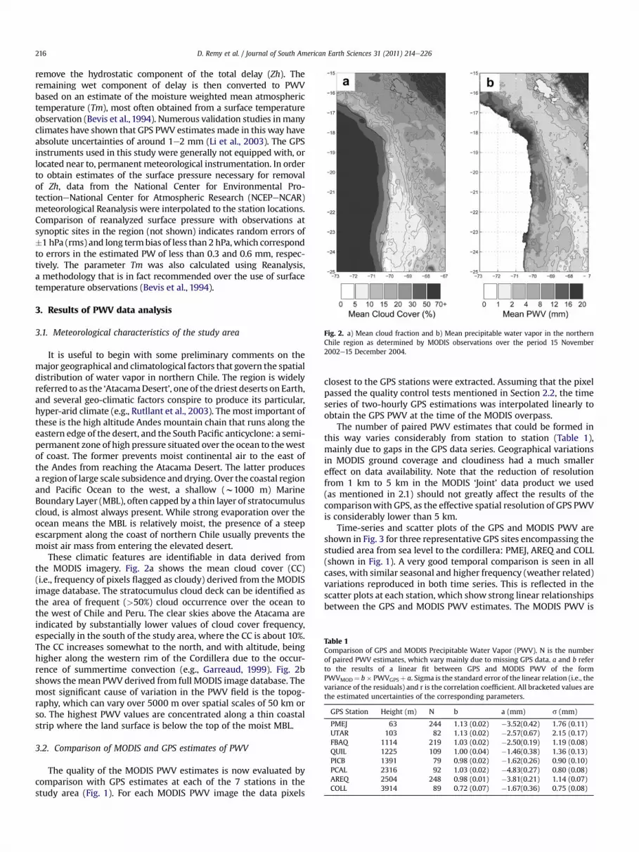
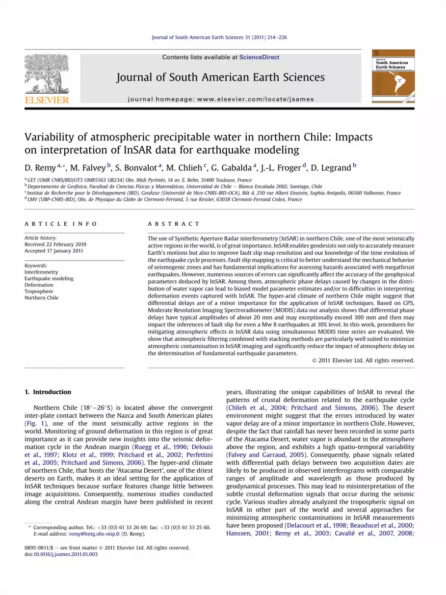
Fig. 2. a) Mean cloud fraction and b) Mean precipitable water vapor in the northernChile region as determined by MODIS observations over the period 15 November2002e15 December 2004.

Table 1Comparison of GPS and MODIS Precipitable Water Vapor (PWV). N is the numberof paired PWV estimates, which vary mainly due to missing GPS data. a and b referto the results of a linear fit between GPS and MODIS PWV of the formPWVMOD¼ b� PWVGPSþ a. Sigma is the standard error of the linear relation (i.e., thevariance of the residuals) and r is the correlation coefficient. All bracketed values arethe estimated uncertainties of the corresponding parameters.

GPS Station Height (m) N b a (mm) s (mm)

PMEJ 63 244 1.13 (0.02) �3.52(0.42) 1.76 (0.11)UTAR 103 82 1.13 (0.02) �2.57(0.67) 2.15 (0.17)FBAQ 1114 219 1.03 (0.02) �2.50(0.19) 1.19 (0.08)QUIL 1225 109 1.00 (0.04) �1.46(0.38) 1.36 (0.13)PICB 1391 79 0.98 (0.02) �1.62(0.26) 0.90 (0.10)PCAL 2316 92 1.03 (0.02) �4.83(0.27) 0.80 (0.08)AREQ 2504 248 0.98 (0.01) �3.81(0.21) 1.14 (0.07)COLL 3914 89 0.72 (0.07) �1.67(0.36) 0.75 (0.08)

D. Remy et al. / Journal of South American Earth Sciences 31 (2011) 214e226216

remove the hydrostatic component of the total delay (Zh). Theremaining wet component of delay is then converted to PWVbased on an estimate of the moisture weighted mean atmospherictemperature (Tm), most often obtained from a surface temperatureobservation (Bevis et al., 1994). Numerous validation studies inmanyclimates have shown that GPS PWV estimates made in this way haveabsolute uncertainties of around 1e2 mm (Li et al., 2003). The GPSinstruments used in this study were generally not equipped with, orlocated near to, permanent meteorological instrumentation. In orderto obtain estimates of the surface pressure necessary for removalof Zh, data from the National Center for Environmental Pro-tectioneNational Center for Atmospheric Research (NCEPeNCAR)meteorological Reanalysis were interpolated to the station locations.Comparison of reanalyzed surface pressure with observations atsynoptic sites in the region (not shown) indicates random errors of�1 hPa (rms) and long termbias of less than 2 hPa,which correspondto errors in the estimated PW of less than 0.3 and 0.6 mm, respec-tively. The parameter Tm was also calculated using Reanalysis,a methodology that is in fact recommended over the use of surfacetemperature observations (Bevis et al., 1994).

3. Results of PWV data analysis

3.1. Meteorological characteristics of the study area

It is useful to begin with some preliminary comments on themajor geographical and climatological factors that govern the spatialdistribution of water vapor in northern Chile. The region is widelyreferred to as the ‘AtacamaDesert’, one of the driest deserts on Earth,and several geo-climatic factors conspire to produce its particular,hyper-arid climate (e.g., Rutllant et al., 2003). The most important ofthese is the high altitude Andes mountain chain that runs along theeastern edge of the desert, and the South Pacific anticyclone: a semi-permanent zone of high pressure situated over the ocean to thewestof coast. The former prevents moist continental air to the east ofthe Andes from reaching the Atacama Desert. The latter producesa region of large scale subsidence and drying. Over the coastal regionand Pacific Ocean to the west, a shallow (w1000 m) MarineBoundary Layer (MBL), often capped by a thin layer of stratocumuluscloud, is almost always present. While strong evaporation over theocean means the MBL is relatively moist, the presence of a steepescarpment along the coast of northern Chile usually prevents themoist air mass from entering the elevated desert.

These climatic features are identifiable in data derived fromthe MODIS imagery. Fig. 2a shows the mean cloud cover (CC)(i.e., frequency of pixels flagged as cloudy) derived from the MODISimage database. The stratocumulus cloud deck can be identified asthe area of frequent (>50%) cloud occurrence over the ocean tothe west of Chile and Peru. The clear skies above the Atacama areindicated by substantially lower values of cloud cover frequency,especially in the south of the study area, where the CC is about 10%.The CC increases somewhat to the north, and with altitude, beinghigher along the western rim of the Cordillera due to the occur-rence of summertime convection (e.g., Garreaud, 1999). Fig. 2bshows themean PWV derived from full MODIS image database. Themost significant cause of variation in the PWV field is the topog-raphy, which can vary over 5000 m over spatial scales of 50 km orso. The highest PWV values are concentrated along a thin coastalstrip where the land surface is below the top of the moist MBL.

3.2. Comparison of MODIS and GPS estimates of PWV

The quality of the MODIS PWV estimates is now evaluated bycomparison with GPS estimates at each of the 7 stations in thestudy area (Fig. 1). For each MODIS PWV image the data pixels

closest to the GPS stations were extracted. Assuming that the pixelpassed the quality control tests mentioned in Section 2.2, the timeseries of two-hourly GPS estimations was interpolated linearly toobtain the GPS PWV at the time of the MODIS overpass.

The number of paired PWV estimates that could be formed inthis way varies considerably from station to station (Table 1),mainly due to gaps in the GPS data series. Geographical variationsin MODIS ground coverage and cloudiness had a much smallereffect on data availability. Note that the reduction of resolutionfrom 1 km to 5 km in the MODIS ‘Joint’ data product we used(as mentioned in 2.1) should not greatly affect the results of thecomparisonwith GPS, as the effective spatial resolution of GPS PWVis considerably lower than 5 km.

Time-series and scatter plots of the GPS and MODIS PWV areshown in Fig. 3 for three representative GPS sites encompassing thestudied area from sea level to the cordillera: PMEJ, AREQ and COLL(shown in Fig. 1). A very good temporal comparison is seen in allcases, with similar seasonal and higher frequency (weather related)variations reproduced in both time series. This is reflected in thescatter plots at each station, which show strong linear relationshipsbetween the GPS and MODIS PWV estimates. The MODIS PWV is

0 10 20 30 400

10

20

30

40

PWGPS (mm)

PWM

OD (m

m)

Q1−04 Q2−04 Q3−04 Q4−040

10

20

30

40

50

PW (m

m)

PMEJ

0 6 12 18 24 300

6

12

18

24

30

PWGPS (mm)

PWM

OD (m

m)

Q1−04 Q2−04 Q3−04 Q4−040

6

12

18

24

30

PW (m

m)

AREQ

0 2 4 6 8 100

2

4

6

8

10

PWGPS (mm)PW

MO

D (m

m)

Q1−04 Q2−04 Q3−04 Q4−040

2

4

6

8

10

PW (m

m)

COLL

Date (starting November 15, 2003)

Fig. 3. Comparison of GPS and MODIS PWV at three selected sites: PMEJ (Mejillones Peninsula, 63 m), AREQ (Arequipa, 2504 m) and COLL (Colina, 3914 m). The panel on the leftshows GPS time series (black) and MODIS PWV estimates (gray) between the 15 November 2002 and 15 December 2004. The right panels show scatter plots of all pairedobservations at each site with the ‘best fit’ linear regression.

D. Remy et al. / Journal of South American Earth Sciences 31 (2011) 214e226 217

consistently lower than the GPS PWV at all three sites, indicative ofbiases in at least one of the two observing systems.

The statistical results presented in Table 1 summarizecomparison between GPS and MODIS PWV at all GPS stationsderived from a standard linear least squares fit the form:PWVMOD þ s ¼ a þ b*PWVGPS which finds the values of zero pointoffset (a), and scaling factor (b) parameters that minimize thestandard deviation of the residual vector (<s>). Ideal values of a,b and <s> are 0, 1 and 0 respectively.

The standard deviations (<s>) vary between 0.75 and 2 mm,with a mean value of 1.3 mm, which compares well to similarstatistics that have been presented in previously publishedcomparisons of MODIS and GPS PWV (e.g., Li et al., 2003). The <s>exhibits a tendency to be highest at moister, low-lying sites, a trendthat can be made clear by plotting variation of <s> with the meanPWV at each site (Fig. 4). We find <s> can be well modeled as thesum of a constant ‘base-line’ random error (s0) and a relative error(sr) whose value is proportional to the PWV (i.e, sr ¼ l PWV).Optimal values for s0 and l are found to be 0.5 and 0.05 (i.e., 50%and 5%) respectively. It is not possible to determine to what extents

MODIS and GPS contribute to the error terms. Both may beexpected to have some degree of constant and relative errors.

At most GPS stations (FBAQ, QUIL, PICB, PCAL and AREQ)the scaling factors (b) are identical to one (95% confidence). Theexceptions are the coastal stations PMEJ (63 m a.s.l) and UTAR(103 m a.s.l), which both have high b parameters of 1.13; and COLL(3914m a.s.l), where b is lowat 0.72. As these stations are at the lowand high altitude extremes of the GPS network, it may be that theb parameter has some altitude dependence. Given the presence ofa negative bias in theMODIS PWV retrievals, values of b< 0 are to beexpected at high altitude points such as COLL, because the zeroboundedMODIS PWV retrieval algorithmmust damp the variabilityof low PWV values. This problem is expected to occur at locationswhere the mean PWV approaches the bias in the MODIS estimates.As discussed in more detail in Li et al. (2003) the presence ofa scaling error in MODIS data parameters will leave a residual errorin corrected interferograms if the MODIS images are left un-calibrated, and an altitude or other dependency of this error willfurther complicate the situation. This error could be substantial. Forexample, the value of b of w0.7 at the COLL site indicates that in

0 5 10 15 20 25 30

0.8

1

1.2

1.4

1.6

1.8

2

2.2

2.4

2.6

PWV (mm)

<φ>

(mm

)

Fig. 4. Standard deviation of the residual <s> of the linear fit between PWVmod andPWVGPS is plotted against the mean PWV at each GPS site. The solid line shows thebest fit curve of a simple model for <s> as the sum of a constant and relative error,i.e, <s> 2 ¼ s2

0 þ (kPWV)2, where s0 and k are 0.5 and 0.05, respectively.

D. Remy et al. / Journal of South American Earth Sciences 31 (2011) 214e226218

extreme cases, the atmospheric phase difference between low andhigh altitude points obtained from MODIS could be overestimatedby as much as 30%. Such extreme case arise for interferograms thatare constructed from one image under very dry (low PWV)conditions and another very moist (high PWV) conditions. Giventhe limited data available in this study we cannot offer any altitudebased correction scheme, and a better sampling at high and lowaltitudes will be necessary to pursue this subject further. None-theless, the good results (b ¼ 1) obtained over large area for themajority of stations indicate that between altitudes of 1000 m and2500 m no external calibration of MODIS data is necessary.

Large negative biases (the a parameters from Table 1), between�1.6 and�3.5 are found at all stations, with no clear pattern in theirspatial variability. The biases are considerably larger than those thathave generally been found in GPS validation studies, suggestingthat the MODIS data have a tendency to underestimate PWV overAtacama region, perhaps due to an unusually high reflectivity of itsdesert surface. For the purpose of InSAR processing, biases of thissort are of minor importance because the time constant errors tendto cancel when forming an interferogram (i.e., the difference ofphase measurements between two different Single Look Complex(SLC) images).

3.3. Evaluation of water vapor effects on SAR interferograms

In this section we examine the likely magnitude of atmosphericeffects on SAR imagery in the Atacama region using the nowvalidated database of MODIS PWV. For the demonstrative purposeof this study, and in order to better match with the horizontaldimension of SAR images, we focus on a relatively small section(w300 km � 300 km), of the overall study area, roughly centeredbetween Mejillones peninsula and the Salar of Atacama. This areabeing also the site of the last magnitude 8 earthquake that occurredin the studied area (Antofagasta, Mw 8.1; July 30, 1995), as dis-cussed later in this paper.

The two-way SAR slant path signal delay (SPD) induced byatmospheric water vapor may be given by (Zebker et al., 1997):

SPD ¼ PWVPcosqinc

(1)

where the SPD is expressed in mm, PWV is the precipitable watervapor (mm) and qinc is the incidence angle of the SAR radar beam. pis an atmospheric parameter that depends on the meteorologicalprofile of pressure, temperature and moisture along the radarbeam path (Bevis et al., 1996). However, since the variability of p isgenerally more than an order of magnitude lower that of the PWV,to a first approximation pmay be treated as a constant with a valueof about 0.15. Since the phase of an interferogram is the differenceof phase between two different SAR images, the slant path delayphase difference (DSPD) is given by:

DSPD ¼ ðPWVt1 � PWVt2ÞPcosqinc

(2)

where DSPD is in mm, and PWVt1 and PWVt2 are the precipitablewater vapor (mm) at the observation times t1 and t2, respectively.This equation shows that what matters to an interferogram is thechange in distribution of PWV from scene to scene rather than theabsolute value of PWV for a particular scene.

From the original database of MODIS images, we selected allthose which were more than 85% complete coverage over the studyarea. A total of 300 images were retained. We used a Monte Carloapproach for simulating interferometric phase screens from randomcombinations of 300 MODIS images. From the original pool, weformed a large set of 1000 randomly selected image pairs. For eachimage pair, we computed the PWV difference (PWVt1 � PWVt2)between the two acquisitions andwe related it to the predicted slantphase delay (DSPD) using the Eq. (2), assuming a nominal meanincidence angle (qinc) of 23� corresponding to the ERS and ENVISAT(swath 2) satellites. At a given pixel the DSPD is evaluated withrespect to an arbitrary chosen reference point located in the Salar ofAtacama (68�17’W, 23�17’S). Fig. 5a and b showmaps of the medianand 95% percentiles of DSPD. The median may be interpreted asrepresenting the level of atmospheric signal in a ‘typical’ (mostprobable) interferogram. The 95% percentiles may be interpreted as‘bad luck’ cases when atmospheric contamination is unusually largebut nonetheless plausible. These maps give a good indication of theexpected tropospheric noise in interferograms computed over thestudy area. They reveal that the amplitude of atmospheric phasedelay in ERS or ENVISAT (swath 2) radar Line-of-Sight (LOS) usuallyreaches about 20e30 mm between the coast and the Salar deAtacama reference point in themedian value cases (Fig. 5a) andmaybe as high as 100mm in the 95% percentiles cases (Fig. 5b). Along thecoast the spatial gradients in DSPD are highest, reaching the equiv-alent of 2 fringes in C-band interferograms, which puts significantlimitations on the measurement of subtle crustal deformations insingle interferograms.

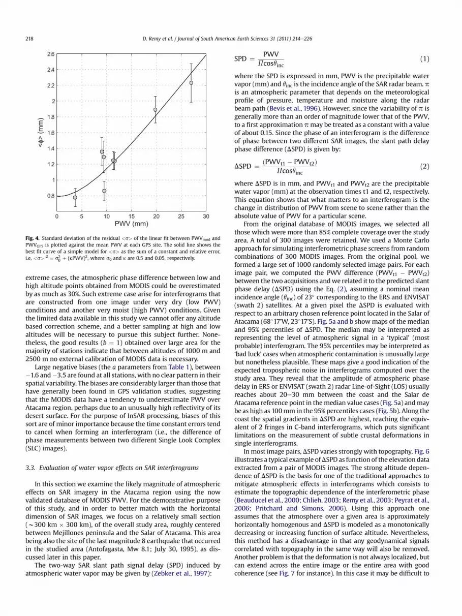
In most image pairs, DSPD varies strongly with topography. Fig. 6illustrates a typical example ofDSPD as functionof the elevation dataextracted from a pair of MODIS images. The strong altitude depen-dence of DSPD is the basis for one of the traditional approaches tomitigate atmospheric effects in interferograms which consists toestimate the topographic dependence of the interferometric phase(Beauducel et al., 2000; Chlieh, 2003; Remy et al., 2003; Peyrat et al.,2006; Pritchard and Simons, 2006). Using this approach oneassumes that the atmosphere over a given area is approximatelyhorizontally homogenous and DSPD is modeled as a monotonicallydecreasing or increasing function of surface altitude. Nevertheless,this method has a disadvantage in that any geodynamical signalscorrelated with topography in the same way will also be removed.Another problem is that the deformation is not always localized, butcan extend across the entire image or the entire area with goodcoherence (see Fig. 7 for instance). In this case it may be difficult to

Fig. 5. Median absolute value of the DSPD with respect to a reference point located on Salar de Atacama taken from 1000 member Monte Carlo sample of random image pairs froma pool of 300 nearly complete MODIS images and their 95% confidence intervals. The black box in a) places the location of the interferograms composed from images taken on thedescending satellite track 96 shown in Fig. 7). a) Median absolute value of the DSPD without removing the elevation dependence. Note the fine scale DSPD patterns, which areobserved along the coast in particularly on the Mejillones Peninsula and on the Salar del Carmen and the salar de Navidad. b) The upper 95% percentile of the DSPD distributionindicating high atmospheric contamination. a’ and b’ are the median absolute value of DSPD after removing the elevation dependence using a generalized spline approximationfrom the DSPD field map shown in a and the corresponding upper 95% percentile of the DSPD distribution. Note the different color scale change between aea’ and beb’ toemphasize difference. The elevation of the study area is represented by white contour lines at 500-m intervals.

−100 −50 0 50 100 1500

1000

2000

3000

4000

5000

6000

Differential Slant Path Delay (ΔSPD) expressed in mm

Altitu

de

(m

)

Fig. 6. Example of altitude dependence of DSPD calculated for two randomly selectedimages. The systematic variation can be reasonably well approximated by a cubicspline. Nevertheless, it is notable that at lower elevation the relation between DSPDand topography is less well defined. This is mainly due to horizontal variation of thePWV along the coast.

D. Remy et al. / Journal of South American Earth Sciences 31 (2011) 214e226220

discriminate ground displacement contributions from the atmo-spheric signal. The availability of global PWV measurementssince the launch of satellite solar spectrometers provided evidenceof more complex behavior and offers alternative approaches forreducing atmospheric effects.

Because the vertical stratification of water vapor is effectivelyarbitrary, there is no physically based model for the differentialdelay induced by atmospheric water vapor. As such, the elevationdependent part of DSPD must be modeled as an arbitrary function

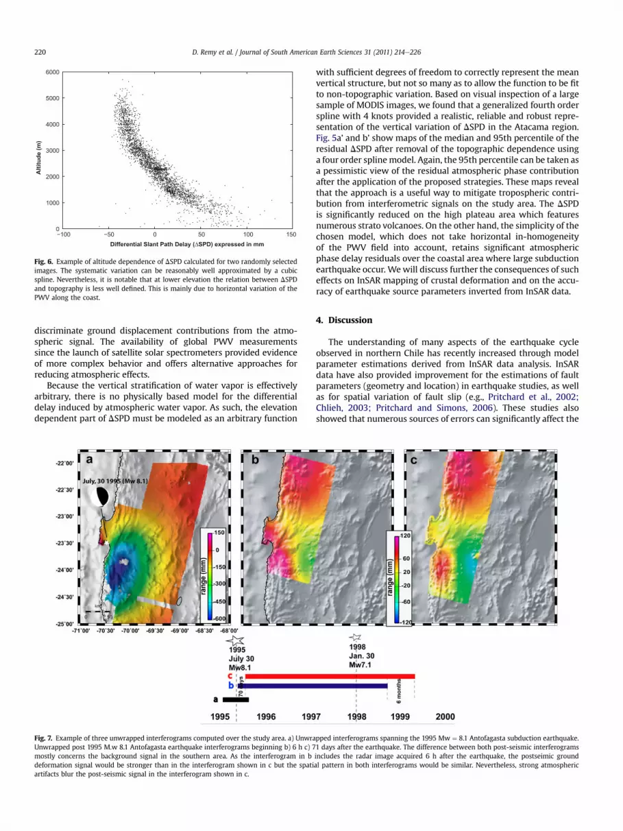
Fig. 7. Example of three unwrapped interferograms computed over the study area. a) UnwraUnwrapped post 1995 M.w 8.1 Antofagasta earthquake interferograms beginning b) 6 h c) 7mostly concerns the background signal in the southern area. As the interferogram in bdeformation signal would be stronger than in the interferogram shown in c but the spatiartifacts blur the post-seismic signal in the interferogram shown in c.

with sufficient degrees of freedom to correctly represent the meanvertical structure, but not so many as to allow the function to be fitto non-topographic variation. Based on visual inspection of a largesample of MODIS images, we found that a generalized fourth orderspline with 4 knots provided a realistic, reliable and robust repre-sentation of the vertical variation of DSPD in the Atacama region.Fig. 5a’ and b’ show maps of the median and 95th percentile of theresidual DSPD after removal of the topographic dependence usinga four order splinemodel. Again, the 95th percentile can be taken asa pessimistic view of the residual atmospheric phase contributionafter the application of the proposed strategies. These maps revealthat the approach is a useful way to mitigate tropospheric contri-bution from interferometric signals on the study area. The DSPDis significantly reduced on the high plateau area which featuresnumerous strato volcanoes. On the other hand, the simplicity of thechosen model, which does not take horizontal in-homogeneityof the PWV field into account, retains significant atmosphericphase delay residuals over the coastal area where large subductionearthquake occur. Wewill discuss further the consequences of sucheffects on InSAR mapping of crustal deformation and on the accu-racy of earthquake source parameters inverted from InSAR data.

4. Discussion

The understanding of many aspects of the earthquake cycleobserved in northern Chile has recently increased through modelparameter estimations derived from InSAR data analysis. InSARdata have also provided improvement for the estimations of faultparameters (geometry and location) in earthquake studies, as wellas for spatial variation of fault slip (e.g., Pritchard et al., 2002;Chlieh, 2003; Pritchard and Simons, 2006). These studies alsoshowed that numerous sources of errors can significantly affect the

pped interferograms spanning the 1995 Mw ¼ 8.1 Antofagasta subduction earthquake.1 days after the earthquake. The difference between both post-seismic interferogramsincludes the radar image acquired 6 h after the earthquake, the postseimic groundal pattern in both interferograms would be similar. Nevertheless, strong atmospheric

D. Remy et al. / Journal of South American Earth Sciences 31 (2011) 214e226 221

accuracy of the geophysical parameters deduced by InSAR.Pritchard et al. (2007) showed that change in velocity model,the fault parameterization (e.g. number, size and dip of subfaults),the inversion strategy (e.g. weighting of a smoothing operator) canimpact geodetic moment by 10% or larger. Atmospheric phasedelays can also lead to biased model parameter estimates or/and todifficulties in interpreting deformation events capturedwith InSAR.The analysis of our large database of MODIS image gave evidencethat phase delays variations may exceptionally exceed 100 mm andmore typically reach about 20 mm and that the vertical variation ofwater vapor induced path delay dominates the spatial pattern. Theamplitude of atmospheric effects in the study area are so much lessthan the coseismic deformation from earthquakes with magnitude>7 such as those occurred in 1995 and 1998 (tens of centimeters).Nevertheless, these effects can lead to difficulties in interpretingdeformation events captured with InSAR.

The Mw 8.1 Antofagasta earthquake of July 30, 1995 was thelargest subduction earthquake that occurred in northern Chile in theXXth century and has been extensively studied from seismic dataand geodetic (InSAR and GPS) measurements (Ruegg et al., 1996;Delouis et al., 1997; Klotz et al., 1999; Pritchard et al., 2002; Chliehet al., 2004). The unwrapped interferograms of this earthquakeindicate major crustal deformation that reaches up to 600 mmof increasing range change in the LOS of the ERS-radar (Fig. 7).The 1995 Antofagasta earthquake was followed in January 30, 1998by the Mw¼ 7.1 earthquake. Two unwrapped interferograms of thisevent were computed using two ERS-radar passes separatedrespectively by 3.6 years (Pair 1, 7b) and 3.3 years (pair 2, 7c). Pair 1starts 6 h after the 1995 main shock and therefore includes most ofthe post-seismic deformation. Pair 2 starts 70 days after the earth-quake. Both interferograms exhibit two different displacementpatterns separated by the Mejillones Peninsula. The signal coveringthe north of the Peninsula is similar in both pairs and was inter-preted as interseismic loading (Chlieh et al., 2004). South of theMejillones Peninsula, the signal is composed of an uplift (decreasingrange) flanked far inland by a subsidence (increasing range) witha gradient of about 120 mm in Pair 1 and about 100 mm in Pair 2.This signal was interpreted as a superposition of the coseismicdeformation of the 1998 Mw ¼ 7.1 earthquake (contribution of 60%of the total signal) and post-seismic deformation that follows the1995 Mw ¼ 8.1 Antofagasta earthquake (Pritchard and Simons,2002; Chlieh et al., 2004). One discrepancy that appears betweenpair 1 and pair 2 was a persistent shift between the two signals ofabout 40 mm that could not be explained by any consistent tectonicmodel. Chlieh (2003) suggested that moisture which is oftentrappedwithin local topographic depression of the Salar del Carmenand the Salar de Navidad could explain such effects (see alsoSection 3.3 and Fig. 5). The persistent shift observed betweenpair 1 and pair 2 interferograms falls in the range of the atmosphericphase delays measured in this study (20e100 mm) and then theatmospheric phase delay may be a consistent explanation toreconcile the discrepancy that appeared between pair 1 and pair 2interferograms.

In the remainder of the paper, we will focus on the impact ofthese atmospheric phase delays on the determination of twofundamental earthquake source parameters: (i) the geodeticmoment and (ii) the slip distribution on the coseismic fault planededuced from single interferograms analysis. We will thus eval-uate the potential and the effectiveness of atmospheric filteringbased on the tropospheric delay-elevation relationship. In orderto prescribe the magnitude of atmospheric delay errors we used1000 randomly selected images of DSPD (described previously inSection 3.3). We applied this approach to the analysis of the faultrupture and slip distribution of the 1995 Mw ¼ 8.1 Antofagastaearthquake.

4.1. Uncertainty analysis of geodetic moment estimation

The seismic moment is a classical quantity used in seismology tomeasure the size of an earthquake and is derived from seismicobservations (short and long period). With the advent of geodeticinstruments (GPS and InSAR), the source of an earthquake could bedetermined from the inversion of geodetic data, and the momentassociated is called the geodetic moment. Its expression (M0) is givenbyM0¼ m SDu,where m is the shearmodulus of themedium involvedin the earthquake, S is the area of the rupture along the geologicfault and Du is the average displacement within the fault area.The assessment of the atmosphere-induced uncertainties of theestimated geodetic moment derived from InSAR observations can beundertaken by inverting the series of DSPD images. Thus DSPD dataare here considered asdeformation signal and inverted. As for surfacedisplacements induced by fault dislocation, eachDSPD surfacefield ismodeled using a single dislocationwithin a homogeneous elastic halfspace (Okada, 1992). The fault parameters are fixed using the valuesproposed by Delouis et al. (1997) except the slip which is set to befree. The inversion then yields the error of the slip displacementrelated to tropospheric signals observed byMODIS and then the erroron the geodetic moment estimation. The result of this simpleapproach indicates that the variability of the atmospheric phasescreen in the study area leads to amedian absolute error of 12 cmanda standard deviation of 24 cm in the determination of the slipdisplacement deduced from InSARmeasurements. This could triggeran error up to 3.3 � 1027 dyn cm at a 95% confidence level in thedetermination of the seismic moment of the 1995 July 30 Mw ¼ 8.1Antofagasta earthquake. Pritchard et al. (2002) proposed a geodeticmoment of 24 � 1027 dyn cm. This result shows that troposphericsignal could induce a bias of about 10% on the inferred slipdisplacement for an earthquake ofmagnitudeMw¼ 8 deduced fromInSAR data.

As vertical stratification is dominant in the study area, weapplied the same strategy as described above, but using as inputdata our set of DSPD images with the elevation dependant partremoved. This simple approach significantly reduces the error inthe determination of the fault slip magnitude: the median error isreduced to about 1 cm with a standard deviation of 2 cm and theerror in the determination of the geodetic moment is reduced to1.3 � 1026 dyn cm at a 95% confidence level.

4.2. Uncertainty analysis of the slip distribution estimation

Although uniform slip models can provides useful information(in particular concerning the geometry of the fault plane), it is wellknown that homogeneous slip along the fault plane is not physi-cally reasonable. InSAR data provides dense and accuratemeasurements of the deformation field which makes it possible todetermine the distribution of slip along the fault plane. To furtherexplore the accuracy of InSAR-derived model for the earthquake,we now focusmore precisely on the impact of atmospheric signal inthe determination of the coseismic slip distribution along the faultplane. We thus fixed the geometry and the discretization of thefault plane into patches using the fault plane model for the Mw 8.1Antofagasta earthquake proposed by (Pritchard et al., 2002). Wedecided to fix the rake angle to 113�, which is the mean value foundby the authors for the fault patches with the best constrained slip.By fixing the geometry, the inversion for the amplitude of the slipbecomes linear and is given by the equation Gm ¼ d, where m isa vector of the amplitude of the slip on each patch, d is the vector ofthe induced tropospheric phase delays and G is the matrix of Greenfunctions for each fault patch computed using an isotropic elastichalf-space model (Okada, 1992). We use a least-square constrainedlinear inversion (CLS) which is part of the MATLAB Optimization

D. Remy et al. / Journal of South American Earth Sciences 31 (2011) 214e226222

Toolbox (Gill et al., 1991) to resolve the slip distribution. We eval-uated the robustness of the approach as follows. We generatedsynthetic data corresponding to null displacements, adding anuncorrelated Gaussian noise with standard deviation of 50 mm andthen inverting the synthetic data for the fault slip. The maximumresulting error for the slip is about 20 mm.

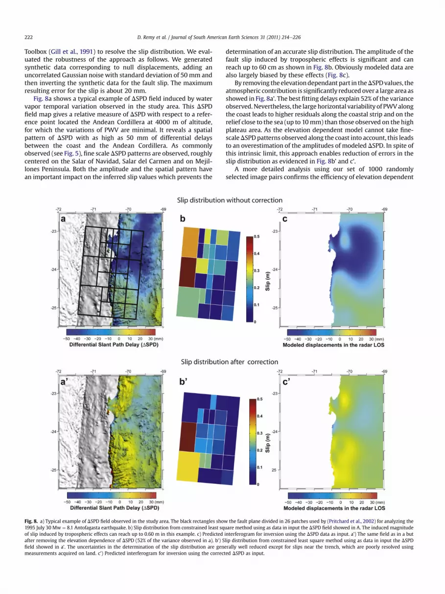
Fig. 8a shows a typical example of DSPD field induced by watervapor temporal variation observed in the study area. This DSPDfield map gives a relative measure of DSPD with respect to a refer-ence point located the Andean Cordillera at 4000 m of altitude,for which the variations of PWV are minimal. It reveals a spatialpattern of DSPD with as high as 50 mm of differential delaysbetween the coast and the Andean Cordillera. As commonlyobserved (see Fig. 5), fine scale DSPD patterns are observed, roughlycentered on the Salar of Navidad, Salar del Carmen and on Mejil-lones Peninsula. Both the amplitude and the spatial pattern havean important impact on the inferred slip values which prevents the

Fig. 8. a) Typical example of DSPD field observed in the study area. The black rectangles sho1995 July 30 Mw ¼ 8.1 Antofagasta earthquake. b) Slip distribution from constrained least sqof slip induced by tropospheric effects can reach up to 0.60 m in this example. c) Predictedafter removing the elevation dependence of DSPD (52% of the variance observed in a). b’) Sfield showed in a’. The uncertainties in the determination of the slip distribution are genmeasurements acquired on land. c’) Predicted interferogram for inversion using the correc

determination of an accurate slip distribution. The amplitude of thefault slip induced by tropospheric effects is significant and canreach up to 60 cm as shown in Fig. 8b. Obviously modeled data arealso largely biased by these effects (Fig. 8c).

By removing theelevationdependant part in theDSPDvalues, theatmospheric contribution is significantly reducedover a large area asshowed in Fig. 8a’. The best fitting delays explain 52% of the varianceobserved.Nevertheless, the largehorizontal variability of PWValongthe coast leads to higher residuals along the coastal strip and on therelief close to the sea (up to 10mm) than those observed on the highplateau area. As the elevation dependent model cannot take fine-scaleDSPDpatterns observed along the coast into account, this leadsto an overestimation of the amplitudes of modeled DSPD. In spite ofthis intrinsic limit, this approach enables reduction of errors in theslip distribution as evidenced in Fig. 8b’ and c’.

A more detailed analysis using our set of 1000 randomlyselected image pairs confirms the efficiency of elevation dependent

w the fault plane divided in 26 patches used by (Pritchard et al., 2002) for analyzing theuare method using as data in input the DSPD field showed in A. The induced magnitudeinterferogram for inversion using the DSPD data as input. a’) The same field as in a butlip distribution from constrained least square method using as data in input the DSPDerally well reduced except for slips near the trench, which are poorly resolved usingted DSPD as input.

D. Remy et al. / Journal of South American Earth Sciences 31 (2011) 214e226 223

model to reduce uncertainties in the determination of the slipdistribution. This analysis also emphasizes the limitation of such anapproach. Fig. 9 gives the absolute value of the median error on thedetermination of each patch slop deduced from the CLS inversionsof the set of 1000 randomly selected image pairs without (9a)or after removal of the elevation dependent part (9a’) and their95% confidence intervals (9b and 9b’). We obtain median absoluteerrors ranging between about 0.10 and 0.40 m and 0.05e0.20 mwithout or after removal of the elevation dependent part in theDSPD values, respectively. In both cases the confidence intervals arelarge (9b, 9b’) and indicate the high variability of the noise struc-ture from one SPD image to other related to atmospheric hetero-geneities in the study area. Even though the elevation dependentmodel reduces the uncertainties in the determination of the slipdistribution, they remain high.Twomain reasons explain these highuncertainties. The one is that not all the fault patch are equallywell resolved because MODIS data, in the same way as InSAR data,are limited to be on land and therefore the slip distribution is poorlyresolved offshore. Furthermore, the variation of troposphericdelays induced by the horizontal variability of the atmosphere,which is not taken into account in our approach, could seriously

0

0.1

0.2

0.3

0.4

med

ian

erro

rs (

m)

1

0.8

0.6

0.4

0.2

0

95 %

per

cent

ile o

f erro

rs (

m)

Single interferogram

a a’

b’

Without correction After correction

b

Fig. 9. Error estimations of the slip distribution related to tropospheric effects. (aa’ebb’) Einterferograms. They are computed from the CLS inversion of the set of 1000 randomly selecshow absolute values of the median slip distribution without or after removal of the elevatintervals of the slip distribution obtained before and after removed the elevation dependantdistribution are generally reduced after removal the elevation dependant part in each DSPby the horizontal variability of the atmosphere. Figure cc’edd’ show error estimations ofinterferograms. They are computed from the CLS inversion of the set of 500 randomly stacksshow the absolute values of the median slip distribution without or after removal of the elevthe 95% confidence intervals of the slip distribution obtained before and after removed thuncertainties in the determination of the slip distribution are well reduced after removal thebetween Figure [aea’,cec’] and Figure [beb’,ded’] in order to better contrast the different

limits the precision of two pass interferometry data to determineaccurate fault slips distribution for a big earthquake.

4.3. Potential of multi-temporal InSAR methods

The analysis of the realistic atmospheric noise upon inversion ofgeophysical parameter presented above provides an incompletepicture because it only involves the analysis of single interfero-grams. Promising results have instead been proven by using mul-ti-image information (Ferretti et al., 2001; Berardino et al., 2002;Usai, 2003; Simons and Rosen, 2007). The most commonapproach consists of reducing the contribution of the atmosphericphase delays by averaging several independent SAR interferograms(Simons and Rosen, 2007). Stacking in general degrades thetemporal resolution of InSAR measurements and this approachmakes it difficult to detect short-lived transient displacements but itis a very good approach to study earthquake or deformation processapproximately linear in time. This method is a reliable approach tominimize atmospheric contamination as it can reduce the varianceof atmospheric error by a factor of N (where N is the number ofindependent interferograms).

0

0.1

0.2

0.3

0.4

1

0.8

0.6

0.4

0.2

0

Stacking of 4 images

c c’

d d’

med

ian

erro

rs (

m)

95 %

per

cent

ile o

f erro

rs (

m)

Without correction After correction

rror estimations of the slip distribution related to tropospheric effects using a singleted image pairs. Each DSPD image is considered as a synthetic interferograms. a and a’ion dependant part in the DSPD fields, respectively. b and b’ show the 95% confidencepart in the DSPD fields, respectively. The uncertainties in the determination of the slipD image. Nevertheless, they remain high due to patches poorly resolved offshore andthe slip distribution related to tropospheric effects using a stack of 4 independentof 4 image pairs. Each DSPD image is considered as a synthetic interferograms. c and c’ation dependant part in the DSPD images used in the stacks, respectively. d and d’ showe elevation dependant part in the DSPD images used in the stacks, respectively. Theelevation dependant part in each DSPD image. Note that a different color scale is used

uncertainty maps.

2003 2004 2005 2006 2007 2008 2009

−40

−20

0

20

40

60

80

SP

D d

elays (m

m)

time

2003 2004 2005 2006 2007 2008 2009

−40

−20

0

20

40

60

80

SP

D d

elays (m

m)

time

a

b

Fig. 10. Two-way SAR slant path signal delays induced by atmospheric water vaporsampled at Mejillones Peninsula (see Fig. 5). a). SPD plot here are estimated froma five-year sample of 50 MODIS images and are expressed in respect with a referencepoint located in the Salar of Atacama. This figure illustrates the high variability of wateralong the Chilean coast. The solid line shows the resulting smoothed time series usinga Bartlett window of 300 days length. The temporal fluctuations in the smoothedtime series are about 30 mm in peak to peak amplitude. Consequently, in this case theground motion retrieved from uncorrected interferograms using multi-temporalapproach would be affected by an error of about 30 mm in LOS between the coast andthe Andean Cordillera. Obviously, it is possible to reduce this amplitude by increasingthe filter width. Nevertheless, such an option would also blur both transient and slowground motions related to tectonic activity in the same way. b) The same time series asin a but after removing the elevation dependence. The temporal fluctuations of thesignal are clearly reduced and the smoothed one has now peak to peak amplitude ofabout 5 mm. By comparing a and b it is possible to quantify how topographicallycorrelated atmospheric path delay is effectively removed by smoothing and theimportance to correct such a delay before employing a smoothing approach.

D. Remy et al. / Journal of South American Earth Sciences 31 (2011) 214e226224

In order to assess the efficiently of the stacking approach tomitigate atmospheric errors, we make use of the database of 1000randomly selected image pairs of DSPD to create a set of 500 stacksof 4 independent DSPD images. Fig. 9c and d shows the absolutevalues of the median slip distribution and the 95% confidenceintervals computed from the CLS inversion of this set of data. Thisconfirms awell known result that using interferograms acquired onseveral different dates well minimizes atmospheric contaminationand significantly reduce the uncertainties in the determination ofthe slip distribution estimated by the inversion technique.

The analysis of our large database of MODIS image reveals thatcorrelated component due to vertical-stratified water vapourdistribution often dominates and represents a large part of theInSAR atmospheric phase variability in the study area. Thus, in orderto assess the impact of topographically correlated atmospheric pathdelays in the inference of fault slip using a stacking approach, weinverted again the same dataset but after removing the topographicdependence in each DSPD image (9c’ and 9d’). Visual comparisonbetween results 9cec’ and 9ded’ clearly shows that this samplecorrection applied leads to better results in the determination of theslip distribution along the fault plane. Using such a similarapproach, allowed Pritchard et al (2006) (by selecting a subset ofinterferograms stacked them together) to detect aw1 cm LOS signalfor the April 19, 1996 earthquake in northern Chile.

It should be stressed also that another particularly effective wayto investigate the spatial and temporal evolution of groundmotion isthrough interferometry time series. When multi-temporal datasetis available, two main methodologies could be used to monitordeformation of the Earth’s surface: the permanent scattered (Ferrettiet al., 2001) and the short baseline time series approach (SBAS)(Berardino et al., 2002; Usai, 2003). Both approaches basicallyinvolve the analysis of a long stack of SAR images. In earthquakecycle, most of the elastic strain accumulated at the plate interface ofthe subduction zone accumulated during decades or centuries isreleased suddenly (few seconds or minutes) in a large earthquakeand its aftershocks. So this is a main shortcoming of these methodsas a large number of SAR images are needed to get reliable result.However these approaches could give useful results to survey longduration displacements induced by several processes of energyrelease accompanying large earthquake such as inter or post-seismicdeformation, for instance. In these approaches the atmosphericartifacts are identified through a two-step filtering operation whichis based on the correlation of the atmosphere in space and itsdecorrelation in time. For example, in SBAS approach the atmo-sphere phase component is detected as the result of the cascade ofa low-pass filtering step, performed in the two-dimensional spatialdomain (i.e., azimuth and range) and a high-pass filtering operationwith respect to the time variable. We now focus on the impact ofcorrelated atmospheric path delays to the InSARmeasurements timeseries computed via the SBAS algorithm.

To analyze this impact, we select 50 MODIS images acquired onthe study area, which sample the period 2003 to 2009. The unevensampling of MODIS data is next converted in single path propaga-tion delays using the Eq. (1) with respect to a reference pointlocated in the Salar of Atacama. Based upon the large variability ofPWV at the Mejillones Peninsula shown previously (see Fig. 5), wefollow the temporal evolution of the single path propagation delaysat a point inside the peninsula.

Fig.10a shows the resulting time series of single path propagationdelays for this selected point. The variability of PWV induces largeamplitude dispersion in the data distribution and a fluctuation ofabout 100 mm in peak to peak amplitude. The temporal timeseries composed of 50 irregularly spaced samples is then smoothedby using a Bartlett window of a length 300 days. The resultingsmoothed time series could be directly compared with the

unsmoothed one. Vertical variation of PWV induced path delay iseffectively reduced to peak to peak amplitude of about 30 mm.Nevertheless, this implies the ground motion retrieved aftertemporal smoothing could be affected by an error of about 30mm inLOS between the coast and the cordillera. So residual troposphericsignal remains in smoothed InSAR time series and could seriouslyblur signal related to slow deformation events such those producedby post or interseimic processes. Next we apply the same strategy asdescribed above but after removing the elevation dependant part inthe time series. The efficiently of the approach is validated by thedecrease in data dispersion in both unsmoothed and smoothedtime series (Fig. 10b). The smoothed signal has now peak to peakamplitude of about 5 mm.

Hence, we conclude that topographically correlated atmosphericpath delays must be estimated and corrected, if possible, in eachinterferogram before employing stacking or smoothing approachesin such a way to better mitigate tropospheric phase delay.

5. Conclusions

Mapping the spatial distribution of fault slip is essential to betterunderstand the mechanisms of the earthquake processes and themechanical behavior of the upper layers of the Earth. The spatial

D. Remy et al. / Journal of South American Earth Sciences 31 (2011) 214e226 225

distribution and quantification of seismic and/or aseismic slip alongthe subduction zone and consequently the degree of inter-plateseismic coupling at the plate interface parallel to the trench hasimportant implications for evaluating the potential of neighboringfault to generate future earthquakes. Due to the low density ofground based monitoring networks in most part of the Chileansubduction margin, InSAR is the main alternative for geodesists toproduce the most accurate maps of the Earth’s surface displace-ment related to subduction processes. The scope of this paper wasto give a quantitative understanding of the impact of atmosphericnoise upon the estimation of the distribution of fault slip andgeodetic moment by InSAR. Our main conclusions could besummarized as follows:

(i) The comparison between MODIS and GPS derived PWV esti-mations in northern Chile shows that both estimates are ingood agreement. The mean standard deviation of 1.3 mmcompares well with similar statistics presented in previousstudies (Li, 2004). Consequently, over a large part of northernChile no external calibration of MODIS data is necessary andPWV estimates show promise as an independent means ofestimating the atmospheric component in InSAR imagescollected in this area.

(ii) The analysis of a one-year database of MODIS image allowed usto characterize both the pattern and the amplitude of expectedtropospheric signal in SAR interferograms on the Salar de Ata-cama region fromelevations between0 to over 5000m. It revealsthat the vertical variation of water vapor induced path delaydominates the spatial pattern in the study area. This analysis alsoreveals that phase delay variations usually reach about 20mm inthe study area and in exceptional cases can reach up to 100 mm.Such effects could be comparable in magnitude and wavelengthwith surface displacements produced by typical subductionearthquake of moderate magnitude (shallow Mw w6 or deepMw w7 earthquake) or post-seismic deformation that followslarge Mw w8 earthquake.

(iii) Our result shows that tropospheric signal could induce a biasof about 10% on the inferred slip displacement deduced fromInSAR data for an earthquake of magnitude Mw ¼ 8 in thestudy area. PWV induced path delay can affect the accuracy ofthe geophysical parameters deduced by inversion of InSARdata in the same order of magnitude than other errors sourcessuch as change in velocity model, fault parameterization(e.g. number, size, dip of subfaults) or inversion strategy.

(iv) Our study shows that the effectiveness of the stacking or SBAStechniques is improvedwhen a traditional atmosphericfilteringbased on the tropospheric delay-elevation relationship is usedto reduce the dispersion in time series of InSAR measurements.This result, in agreement with other studies (Peyrat et al., 2006;Pritchard and Simons, 2006; Cavalié et al., 2008; Elliott et al.,2008; Doin et al., 2009), confirms that even using time seriesof SAR images, topography correlated atmospheric delays mustbe estimated and corrected, if necessary.

(v) Even if it could be possible to estimate topography correlatedtropospheric effects directly from the interferograms, thismethod has a disadvantage in that any geodynamical signalscorrelated with topography in the same way will be removed.In this context, satellite based PWV estimates offer a reliablealternative means to discriminate displacement contributionsfrom the atmospheric signal.

Our approach in this paper has not provided a ready-madesolution tomitigate the tropospheric contribution in InSAR data butrather has quantified their consequences in the context of earth-quake studies. Atmospheric effects remain one of the limiting error

sources in the use of InSAR techniques and further works are stillnecessary to develop more effective methods to mitigate theireffects in geophysical studies.

Acknowledgments

We wish to thank M. Pritchard for his useful comments andhis encouragement. We thank ENTEL Chile (Iquique), DirecciónGeneral de Aeronáutica Civil de Chile (Iquique), Mineria Dona Inesde Collahuasi, Universidad Arturo Prat, Sernageomin Iquique forthe logistic support for the northern Chile GPS network. The GPSdata were acquired in the frame of the French-Chilean cooperationprogram by IRD, IPG Paris and Department of Geophysics and theSeismological Service of the University of Chile. The MERIS andENVISAT data have been acquired through ESA research projects:ENVISAT A-O n�857 (PI: JL. Froger) and Category 1 research projectN�2899 (PI: S. Bonvalot). This study has been supported by IRD(Dept. DME, DSF), University of Chile (Department of Geophysics/Meteorology) and ECOS-CONICYT (project n�C00U03) FONDECYT-CONICYT (project n� 1030800) and IRD-CONICYT.

References

Beauducel, F., Briole, P., Froger, J.L., 2000. Volcano wide fringes in ERS syntheticaperture radar interferograms of Etna (1992-1999): deformation or tropo-spheric effect? Journal of Geophysical Research 105, 16391e16402.

Bennartz, R., Fischer, J., 2001. Retrieval of columnar water vapour over land frombackscattered solar radiation using the medium resolution imaging spectrom-eter. Remote Sensing of Environment 78, 274e283.

Berardino, P., Fornaro, G., Lanari, R., Sansosti, E., 2002. A new algorithm for surfacedeformation monitoring based on small baseline differential SAR interfero-grams. Geoscience and Remote Sensing, IEEE Transactions on 40, 2375e2383.

Bevis, M., Businger, S., Chiswell, S., Herring, A.T., Anthes, R.A., Rocken, C., Ware, R.H.,1994. GPS Meteorology: mapping zenith wet delays onto precipitable water.Journal of Applied Metereology 33, 379e386.

Bevis, M., Chiswell, S., Businger, S., Herring, T.A., Bock, Y., 1996. Estimating wet delayusing numerical weather analysis and predictions. Radio Science 31, 447e487.

Cavalié, O., Doin, M.-P., Lasserre, C., Briole, P., 2007. Ground motion measurement inthe Lake Mead area, Nevada, by differential synthetic aperture radar interfer-ometry time series analysis: probing the lithosphere rheological structure.Journal of Geophysical Research 112.

Cavalié, O., Lasserre, C., Doin, M.-P., Peltzer, G., Sun, J., Xu, X., Shen, Z.-K., 2008.Measurement of interseismic strain across the Haiyuan fault (Gansu, China), byInSAR. Earth and Planetary Science Letters 275, 246e257.

Chlieh, M., 2003. Le Cycle Sismique décrit avec les données de la Géodésie Spatiale(interférométrie SAR et GPS différentiel): variations spatio-temporelles desglissements stables et instables sur l’interface de subduction du Nord Chili. In:Géophysique Interne. Institut de Physique du Globe de Paris, p. 173.

Chlieh, M., de Chabalier, J.B., Ruegg, J.C., Armijo, R., Dmowska, R., Campos, J., Feigl, K.,2004. Crustal deformation and fault slip during the seismic cycle in the NorthChile subduction zone, from GPS and InSAR observations. Geophysical JournalInternational 158, 695e711.

Delacourt, C., Briole, P., Achache, J., 1998. Tropospheric corrections of SAR inter-ferograms with strong topography. Application to Etna. Geophysical ResearchLetters 25, 2849e2852.

Delouis, B., Monfret, T., Dorbath, L., Pardo, M., Rivera, L., Compte, D., Haessler, H.,Caminade, J.P., Ponce, L., Kausel, E., Cisternas, A., 1997. The Mw 8.0 Antofagasta(Northern Chile) earthquake of 30 July 1995: a precursor to the end of the large1877 gap. Bulletin of the Seismological Society of America 87, 427e445.

Doin, M.P., Lasserre, C., Peltzer, G., Cavalié, O., Doubre, C., 2009. Corrections ofstratified tropospheric delays in SAR interferometry: validation with globalatmospheric models. Journal of Applied Geophysics, in press, [Corrected proof].

Elliott, J.R., Biggs, J., Parsons, B., Wright, T.J., 2008. InSAR slip rate determination onthe Altyn Tagh Fault, northern Tibet, in the presence of topographically corre-lated atmospheric delays. Geophysical Research Letters 35.

Falvey, M., Garraud, R., 2005. Moisture variability over the South American Alti-plano during the SALLJEX observing season. Journal of Geophysical Research110. doi:10.1029/2005JD006152.

Ferretti, A., Prati, C., Rocca, F., 2001. Permanent Scattered in SAR interferometry.IEEE Transactions on Geoscience and Remote Sensing 39, 8e20.

Froger, J.L., Remy, D., Bonvalot, S., Legrand, D., 2007. Two Scales of inflation atLastarria-Cordon del Azufre volcanic complex, central Andes, revaled fromASAR-ENVISAT interferometric data. Earth and Planetery Science Letters.doi:10.1016/j.epsl.2006.12.012.

Gao, B.-C., Kaufman, Y.J., 2003. Water vapor retrieval using Moderate ResolutionImaging Spectroradiometer (MODIS) near-infrared channels. Journal ofGeophysical Research D13. doi:10.1029/2002JD003023.

D. Remy et al. / Journal of South American Earth Sciences 31 (2011) 214e226226

Garreaud, R.D., 1999. A multi-scale analysis of the summertime precipitation overthe central Andes. Monthly Weather Review 127, 901e921.

Gill, P.E., Murray, W., Wright, M.H., 1991. Practical Optimisation. Academic Press,London.

Hanssen, R., 2001. Radar Interferometry Data Interpretation and Errors Analysis.Kluwer Academic Publishers, Dordrecht, The Netherland.

Herring, A.T., King, R.W., McClusky, S.C., 2006a. GPS Analysis at MIT, Gamit Refer-ence Manual, Release 10.3. Massachussetts: M.I.T, Cambridge.

Herring, T.A., King, R.W., McClusky, S., 2006b. Global Kalman Filter VLBI and GPSAnalysis Program, Globk Reference Manual, Release 10.3. Massachussetts: M.I.T,Cambridge.

Klotz, J., Angermann, D., Michel, G.W., Porth, R., Reigber, C., Reinking, J.,Viramonte, J., Perdomo, R., Rios, V.H., Barrientos, S., Barriga, R., Cifuentes, O.,1999. GPS-derived deformation of the central Andes including the 1995 Anto-fagasta Mw ¼ 8.0 earthquake. Pure and Applied Geophysics 154, 709e730.

Li, Z., Muller, J.P., Cross, P., 2003. Comparison of precipitable water vaporderived from radiosonde, GPS and Moderate-resolution Imaging Spectroradi-ometer measurements. Journal of Geophysical Research 108. doi:10.1029/2003JF¼D003372.

Li, Z., 2004. Production of Regional 1 km � 1 km Water Vapor Fileds through theIntegration of GPS and MODIS Data. ION gnss. Inst. of Navig, Long BeachCalifornie. 21e24 Sept.

Loveless, J.P., Pritchard, M.E., 2008. Motion on upper-plate faults during subductionzone earthquakes: case of the Atacama Fault System, northern Chile.Geochemistry, Geophysics, Geosystems 9, Q12017.

Okada, Y., 1992. Internal deformation due to shear and tensile faults in a half-space.Bulletin of the Seismological Society of America 82, 1018e1040.

Pavez, A., Remy, D., Bonvalot, S., Diament, M., Gabalda, G., Froger, J.L., Julien, P.,Legrand, D., Moisset, D., 2006. Insight into ground deformation at lascar volcano(Chile) from SAR interferometry, photogrammetry and GPS data: implication onvolcano dynamics and future space monitoring. Remote Sensing of Environ-ment 100, 307e320.

Perfettini, H., Avouac, J.-P., Ruegg, J.-C., 2005. Geodetic displacements and after-shocks following the 2001 Mw ¼ 8.4 Peru earthquake: implications for themechanics of the earthquake cycle along subduction zones. Geophysical JournalInternational 110.

Peyrat, S., Campos, E., de Chabalier, J.B., Perez, A., Bonvalot, S., Bouin, M.-P.,Legrand, D., Nercessian, A., Charade, O., Patau, G., Clevede, E., Kausel, E.,Bernard, P., Vilotte, J.-P., 2006. The Tarapaca intermediate-depth earthquake(Mw 7.7, 2005, Northern Chile): a slab-pull event with horizontal fault plane

constrained from seismologic and geodetic observations. Geophysical ResearchLetters 33. doi:10.1029/2006GL027710.

Pritchard, M.E., Simons, M., 2002. A satellite geodetic survey of large scale defor-mation of volcanic centres in the central Andes. Nature 418, 167e170.

Pritchard, M.E., Simons, M., Rosen, P.A., Hensley, S., Webb, F.H., 2002. CO-seismicslip from the 1995 July 30 Mw¼8.1 Antofagasta, Chile, earthquake asconstrained by InSAR and GPS obervations. Geophys. J. Int 150, 362e376.

Pritchard, M.E., Simons, M., 2006. An aseismic slip pulse in Northern Chile andalong-strike variation in seismogenic behavior. Journal of Geophysical Research111. doi:10.1029/2006JB004258.

Pritchard, M.E., Norabuena, E.O., Ji, C., Boroschek, R., Comte, D., Simons, M.,Dixon, T.H., Rosen, P.A., 2007. Geodetic, teleseismic, and strong motionconstraints on slip from recent southern Peru subduction zone earthquakes.Journal of Geophysical Research 112.

Puysségur, B., Michel, R., Avouac, J.P., 2007. Tropospheric phase delay in interfero-metric synthetic aperture radar estimated from meteorological model andmultispectral imagery. Journal of Geophysical Research 112.

Remy, D., Bonvalot, S., Briole, P., Murakami, M., 2003. Accurate measurement oftropospheric effects in volcanic area from SAR interferometry data: applicationto Sakurajima volcano (Japan). Earth and Planetery Science Letters 213,299e310.

Ruegg, J.C., Campos, J., Armijo, R., Barrientos, S., Briole, P., Thiele, R., Arancibia, M.,Cañuta, J., Duquesnoy, T., Chang, M., Lazo, D., Lyon-Caen, H., Ortlieb, L.,Rossignol, J., Serrurier, L., 1996. The Mw ¼ 8.1 Antofagasta (North Chile)earthquake of July 30, 1995: first results from teleseismic and geodetic data.Geophysical Research Letters 23, 917e920.

Rutllant, J.A., Fuenzalida, H., Aceituno, P., 2003. Climate dynamics along the aridnorthern coast of Chile: the 1997-1998 Dinámica del Clima de la Region deAntofagasta (DICLIMA) experiment. Journal of Geophysical Research 108,002003. doi:10.1029/2002JD003357.

Simons, M., Rosen, P., 2007. Treatise on Geophysics, interferometric synthetic aper-ture radar Geodesy. In: Schubert, G.E. (Ed.), Geodesy. Elsevier Press, pp. 391e446.

Tregoning, P., Boers, R., Obrien, D., Hendy, M., 1998. Accuracy of absolute precipi-table water vapor estimates from GPS observations. Journal of GeophysicalResearch 103, 28701e28710.

Usai, S., 2003. A least squares database approach for SAR interferometric data.Geoscience and Remote Sensing, IEEE Transactions on 41, 753e760.

Zebker, H.A., Rosen, P.A., Heinsley, S., 1997. Atmospheric effects in interferometricsynthetic aperture radar surface deformation and topographic maps. Journal ofGeophysical Research 102, 7547e7563.