valuation of siem offshore inc. - cbs research portal
TRANSCRIPT
! ! !!!
!
Valuation of Siem Offshore Inc. Copenhagen Business School, May 2013
Master Thesis
Supervisor: Edward Vali, Copenhagen Business School
Number of standard pages: 119
Number of characters: 229.049
Eivind Kjær Thorsen FIR Henrik Eide Arnesen, FSM

HighB
SIOFF.OLSIOFF:NO
495m2845m672m1167m
390mAverage daily turnover NOK 0.5-1m
Shareprice performance 2005 - 2013
-3mnd -6mnd -9mndReturn -14.4% -7.7% -23.3%Price high 8.5 8.6 9.5Price low 7.2 6.8 7.0
ROCE 2012E 0.8%ROIC 2012E 0.7%EBITDA-Margin 2012E 30%EBIT-Margin 2012E 5%
10.1%
2008H 2009H 2010H 2011H 2012H 2013E 2014E 2015E 2016E
Sales 194,262 184,955 230,326 322,014 309,606 326,166 452,546 556,649 609,732EBITDA 81,216 60,378 82,947 114,286 94,100 113,059 171,257 237,869 269,176NOPAT 41,213 23,603 22,234 4,799 11,445 40,816 82,366 128,879 156,645EPS recuring -0.07 0.26 0.03 -0.02 0.04 0.00 0.06 0.16 0.23Sales growth 21% -5% 25% 40% -4% 5% 39% 23% 10%EBITDA growth 0% -26% 37% 38% -18% 20% 51% 39% 13%EBITDA-margin 42% 33% 36% 35% 30% 35% 38% 43% 44%
Multiples 2013 2014 2013 2014 2013 2014 2013 2014
Siem Offshore Inc. 3.6 2.6 10.4 6.8 24.7 12.2 0.66 0.57Harmonic Average peers 3.3 3.1 8.1 7.3 11.9 10.0 0.52 0.47
Estimates from Investment banksArcitc Securities 13
9.5Fondsfinans 12.5Pareto Securities 12
Average 11.8
Stock price pr. 14.05.2013 7.87AnalystHenrik Eide Arnesen and Eivind Kjær Thorsen
Executive Summary
Siem Offshore Inc. HOLD
Oil Service/Offshore supply 14. May 2013
Enterprice Value, USD
Reuters tickerBloomberg Ticker
Key dataRisk
Target price: NOK 7.6Shareprice 16.04.2013: NOK 7.3
Implied credit rating
Market cap UsdMarket cap NOKNIBD, USD
Shares fully diliuted
SEB Enskilda
EV/Sales P/BEV/EBITDA EV/EBIT
Key figures USD`000
WACC
Not the preferred exposure given our market outlook Siem Offshore Inc. is a strong Norwegian Offshore Supply player with operations in Brazil, West Africa, Gulf of Mexico and the North Sea. The company provides exposure towards the high-end AHTS, PSV and OSCV/MRSV segment with a total fleet of 33 vessels and ten newbuildings. The major driver for SIOFFs revenues is the global offshore E&P spending. Petroleum companies investments is driven by the level of the oil price, and demand for OSVs is positively affected by the number of offshore rigs, platforms and subsea wells. Since the financial crises demand has picked up, but the market continues to be dominated by oversupply. In 2013 global E&P spending is set to increase by 13%, with a high number of rig deliveries. Offshore activity in deepwater areas is the main contributor to this growth, as these operations are complex, driving vessel demand. Brazil and West Africa stands out as the regions with the highest expected growth, and SIOFF provides exposure towards both these markets. Petroleum companies prefer flexibility and quality of operations, and we therefore see a premium of dayrates and utilization going forward. On the other hand we see a strong supply growth, which will limit the upside potential of dayrates. The AHTS and OSCV/MRSV segment is best positioned as there are entry barriers limiting supply growth. However this is not the case for the PSV segment, and SIOFFs fleet of PSVs will experience limited earning growth. SIOFFs financial risk is modest as the balance sheet remains helalthy. Cash reserves is above USD 100m and only Farstad Shipping has a lower financial gearing. Based on our estimated value we see the company as fairly priced, providing a limited upside potential. This is supported by the relative valuation, where SIOFF looks somewhat expensive based on 2013 multiples.
0
5
10
15
20
25
!!
2!!
1.0 Introduction / Motivation ......................................................................................................................................... 4 1.1 Problem statement ................................................................................................................................................... 5 1.2 Models and data collection ..................................................................................................................................... 7 1.3 Delimitation .......................................................................................................................................................... 15
2.0 Introduction to Siem Offshore and the offshore supply vessel (OSV) industry ................................................ 16 2.1 Siem Offshore Inc. ................................................................................................................................................ 16 2.2 The offshore supply market (OSV) ...................................................................................................................... 16 2.3 Major historical events and SIOFFs share price development ............................................................................. 19 2.4 Organization .......................................................................................................................................................... 20 2.5 Management team and board of directors ............................................................................................................. 21 2.6 Ownership structure .............................................................................................................................................. 22 2.7 The SIOFF fleet and business areas ...................................................................................................................... 22 2.8 Contract coverage and utilization ......................................................................................................................... 26 2.9 Geographical segments ......................................................................................................................................... 27 2.10 Definition of peer group ..................................................................................................................................... 28 2.11 Business cycle and state of now ......................................................................................................................... 31
3.0 Strategic analysis ..................................................................................................................................................... 32 3.1 The shipping market model .................................................................................................................................. 32
3.1.1 Demand for OSV ........................................................................................................................................... 32 3.1.1.1 Global oil supply .................................................................................................................................... 33 3.1.1.2 E&P Spending ........................................................................................................................................ 34 3.1.1.3 Components of E&P spending growth ................................................................................................... 36 3.1.1.3 Regional demand .................................................................................................................................... 40 3.1.1.5 Summary – Demand for OSV ................................................................................................................ 41
3.1.2 Supply of OSV ............................................................................................................................................... 42 3.1.2.1 Five decision makers .............................................................................................................................. 42 3.1.2.2 The total World Fleet .............................................................................................................................. 43 3.1.2.3 Newbuilding ........................................................................................................................................... 44 3.1.2.4 Scrapping ................................................................................................................................................ 45 3.1.2.5 Summary Supply .................................................................................................................................... 45
3.1.3 The dayrate mechanism ................................................................................................................................. 46 3.1.4 Conclusion to the shipping market model ..................................................................................................... 50
3.2 Porters Five Forces ............................................................................................................................................... 51 3.2.1 Competition from substitutes ......................................................................................................................... 51 3.2.2 Threat of entry ............................................................................................................................................... 51 3.2.3 Bargaining power of Buyers .......................................................................................................................... 53 3.2.4 Bargaining power of Suppliers ...................................................................................................................... 54 3.2.5 Rivalry between established companies ........................................................................................................ 56 3.2.6 Conclusion ..................................................................................................................................................... 57
3.2.7 Market outlook for the OSV industry ........................................................................................................ 58 3.3 Internal analysis .................................................................................................................................................... 59
3.3.1 Value Chain Approach .................................................................................................................................. 59 3.3.2 VRIO .............................................................................................................................................................. 60
3.3.2.1 Physical resources .................................................................................................................................. 60 3.3.2.2 Individual and Human Resources ........................................................................................................... 62 3.3.2.3 Financial resources ................................................................................................................................. 65 3.3.2.4 Organizational and combined resources ................................................................................................. 65
3.3.3 Conclusion Internal analysis .......................................................................................................................... 66
!!
3!!
4.0 Financial Statement Analysis ................................................................................................................................. 67 4.1 Rebalancing financial statements for analytical purpose ...................................................................................... 68
4.1.2 The analytical income statement ................................................................................................................... 68 4.1.3 The analytical balance sheet .......................................................................................................................... 69
4.2 Analysis of historical profitability and performance ............................................................................................ 70 4.2.1 Operational result – Decomposition of ROIC ............................................................................................... 71 4.2.2 Profit margin .................................................................................................................................................. 72 4.2.3 Turnover rate invested capital ....................................................................................................................... 75
4.2.4.1 Indexing and common-size analysis of invested capital ........................................................................ 75 4.2.5 FGEAR .......................................................................................................................................................... 76 4.2.6 Spread ............................................................................................................................................................ 77 4.2.7 Owners perspective – ROE ............................................................................................................................ 77
4.3 Liquidity Risk Analysis ........................................................................................................................................ 78 4.3.1 Short-term liquidity risk ................................................................................................................................ 78 4.3.2 Long term liquidity risk ................................................................................................................................. 79
4.4 Relative market share and Return on Capital Employed (ROCE) ........................................................................ 81 5.0 SWOT ....................................................................................................................................................................... 82 6.0 Forecasting ............................................................................................................................................................... 83
6.1 Forecasting of dayrates ......................................................................................................................................... 83 6.1.1 Forecasting of dayrates – AHTS segment ..................................................................................................... 83
6.1.1.1 Regression analysis ................................................................................................................................ 83 6.1.1.2 Output Results and Discussion ............................................................................................................... 84 6.1.1.3 The forecast of dayrates .......................................................................................................................... 85
6.1.2 Forecast of dayrates – PSV segment ............................................................................................................. 86 6.1.3 Forecast of dayrates – Subsea ........................................................................................................................ 87
6.2 Forecasting long term contracts, utilization and newbuilds .................................................................................. 88 6.3 Forecasting of future revenues, expenses and cash flow ...................................................................................... 91
6.3.1 Forecast period ............................................................................................................................................... 91 6.3.2 Terminal growth ............................................................................................................................................ 91 6.3.3 Pro forma income statement .......................................................................................................................... 91 6.3.4 Pro forma Balance sheet ................................................................................................................................ 95 6.3.5 Quality of the estimates supporting the pro forma statements ...................................................................... 98
7.0 Estimating cost of capital ...................................................................................................................................... 99 7.1 Return on Equity, re .............................................................................................................................................. 99
7.1.1 Risk free rate, rf .............................................................................................................................................. 99 7.1.2 Systematic risk – beta, β .............................................................................................................................. 100 7.1.3 Equity risk premium .................................................................................................................................... 102 7.1.4 Liquidity premium ....................................................................................................................................... 102
7.2 Return on debt ..................................................................................................................................................... 103 7.3 Capital structure .................................................................................................................................................. 104
8.0 Valuation ................................................................................................................................................................ 106 8.1 Valuation: Discounted Cash Flow approach ....................................................................................................... 106 8.2 Valuation: Economic Value Added .................................................................................................................... 108 8.3 Relative valuation: Multiples .............................................................................................................................. 109
9.0 Sensitivity analysis ................................................................................................................................................ 112 10.0 Discussion ............................................................................................................................................................. 116 11.0 Conclusion ............................................................................................................................................................ 117 12.0 Thesis in perspective ........................................................................................................................................... 119 13.0 Bibliography ........................................................................................................................................................ 120 14.0 Appendix .............................................................................................................................................................. 124
!!
4!!
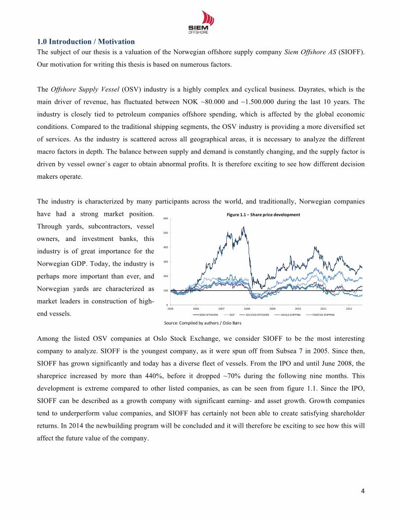
1.0 Introduction / Motivation The subject of our thesis is a valuation of the Norwegian offshore supply company Siem Offshore AS (SIOFF).
Our motivation for writing this thesis is based on numerous factors.
The Offshore Supply Vessel (OSV) industry is a highly complex and cyclical business. Dayrates, which is the
main driver of revenue, has fluctuated between NOK ~80.000 and ~1.500.000 during the last 10 years. The
industry is closely tied to petroleum companies offshore spending, which is affected by the global economic
conditions. Compared to the traditional shipping segments, the OSV industry is providing a more diversified set
of services. As the industry is scattered across all geographical areas, it is necessary to analyze the different
macro factors in depth. The balance between supply and demand is constantly changing, and the supply factor is
driven by vessel owner`s eager to obtain abnormal profits. It is therefore exciting to see how different decision
makers operate.
The industry is characterized by many participants across the world, and traditionally, Norwegian companies
have had a strong market position.
Through yards, subcontractors, vessel
owners, and investment banks, this
industry is of great importance for the
Norwegian GDP. Today, the industry is
perhaps more important than ever, and
Norwegian yards are characterized as
market leaders in construction of high-
end vessels.
Among the listed OSV companies at Oslo Stock Exchange, we consider SIOFF to be the most interesting
company to analyze. SIOFF is the youngest company, as it were spun off from Subsea 7 in 2005. Since then,
SIOFF has grown significantly and today has a diverse fleet of vessels. From the IPO and until June 2008, the
shareprice increased by more than 440%, before it dropped ~70% during the following nine months. This
development is extreme compared to other listed companies, as can be seen from figure 1.1. Since the IPO,
SIOFF can be described as a growth company with significant earning- and asset growth. Growth companies
tend to underperform value companies, and SIOFF has certainly not been able to create satisfying shareholder
returns. In 2014 the newbuilding program will be concluded and it will therefore be exciting to see how this will
affect the future value of the company.
0
100
200
300
400
500
600
2005 2006 2007 2008 2009 2010 2011 2012
SIEM/OFFSHORE DOF SOLSTAD/OFFSHORE HAVILA/SHIPPING FARSTAD/SHIPPING
Figure 1.1)– Share price development
Source:/Compiled by/authors //Oslo/Børs
!!
5!!
1.1 Problem statement The purpose of the thesis is to determine the intrinsic value of Siem Offshore Inc. (SIOFF) by applying different
valuation techniques. Our findings will be summarized in a recommendation to potential investors. We have
formulated the following problem statement:
What is the intrinsic equity value for a marginal investor in Siem Offshore Inc. as of 16.04.2013, compared to the
market capitalization at Oslo Stock Exchange?
Sub questions
In order to answer the statement we will categorize the thesis in different sub-sections. We will conduct different
analysis in each section, by answering a series of sub-question. Our findings will be summarized in partial
conclusions. These partial conclusions will be combined into a final conclusion at the end of the thesis, which
answers the overall problem statement
Introduction to Siem Offshore Inc. and the OSV industry
A thoroughly understanding of the business is necessary, in order to conduct a successful valuation. It is
important to understand the value chain of the petroleum industry, business sector, customers, suppliers and the
service they provide. This will be important input in all the analysis and help us identify the right value drivers.
In this part of the thesis we will answer the following questions:
' What are the main characteristics of SIOFF strategy and the business concept?
' What characterize the OSV market and the clients, and how has the industry developed?
' Who are the main competitors/comparable firms?
Strategic analysis of the OSV market and the company
This part of the thesis serves as an analysis of the non-financial drivers that affect SIOFF. We will analyze how
the business environment and market cycles affect the company´s value creation. The internal factors will
explain how SIOFF exploits market opportunities and adjust to changing market conditions. The analysis will
first look at the macro perspective and the supply/demand balance in relation to the industry structure. In the
internal analysis we will look at the value chain and the company´s resources.
' How is the dayrate mechanism determined by the supply/demand relation?
' How does the industry structure affect the future earnings prospects?
' Does SIOFF hold a competitive advantage?
!!
6!!
Financial analysis
The purpose of the financial analysis is to uncover SIOFFs historical performance, and break down all the
components for further analysis. Future performance is not necessarily equal to historical results, but the latter
can be used as a reference and indicator to the forecasting. In order to get a clear picture of SIOFFs performance
we will benchmark the results to a chosen group of peers.
' How has SIOFF performed financially through the last five years and compared to peers?
' How has SIOFF and peers been affected by the latest downturn in the industry?
' How has the growth rate affected the company´s OPEX?
' What are the prospects for the future financial performance?
Forecasting
In the forecasting the findings from the strategic and financial analysis are tied together to form realistic
projections for the future. Since the valuation model will be based on future cash flow, accuracy and analytical
knowledge will be key components in the forecasting.
' How will SIOFFs key value drivers be affected by the expected market outlook?
' How will the spot market for the different segments develop in the future?
' What is the future CAPEX need, and when is the company likely to reach state of steady growth?
Valuation
There are many different valuation models to choose from, which rely on different set of assumptions. By using
more than one model we will be able to triangulate the result. A common feature of the present value models is
the need of a risk adjusted discount rate. To estimate the equity value, we will use the following sub questions as
a basis:
' What is the proper discount rate for a marginal investor in SIOFF?
' What is the forecasted cash flow from operation?
' How is SIOFF price relative to peers?
' How sensitive is the estimate to changes in general and company specific parameters?
!!
7!!
1.2 Models and data collection
1.2.1 Data collection
This thesis is written from an independent analyst’s point of view, and we have only used publicly available
information. As we will apply both financial and strategic analysis, the data input consists of both quantitative
and qualitative aspects. Our sources of date are annual reports, market data and research from investment banks.
In addition, we will apply different theories from academic books, financial literature, and articles. We have also
conducted phone interviews with shipbrokers, analysts, and industry specialists. Combining all of these
resources, we are confident that we have a sufficient foundation to estimate a fair value of Siem Offshore.
1.2.2 Supply/Demand – The shipping market model
To analyze the macroeconomic environment of the
company there are various strategic models to choose
from. It is important that the choice of model is
applicable for the industry that is analyzed.
In a commodity industry, the relation between demand
and supply is the key factor determining prices. As the
OSV industry is a global business with mobile assets
and a high number of competitors it can be viewed as a
“commoditized industry´”. Together with utilization,
dayrates is the key factor affecting revenue, and the
mechanism determining rates must therefore be
thoroughly analyzed.
We have chosen “The shipping market model”
developed by Martin Stopford in 1997. The purpose of
the model is to identify the main market drivers that
affect the OSV market, and how these influence the
level of dayrates.
The model is intended for analysis of the traditional
shipping markets (bulk, tank, and container).
Supply
Balance'between supplyand'demand;
Dayrates'and'ulitization
Oil'pricedevelopment World'economyRandom Shocks
E&P'Spending
Furtherdemanddrivers
Demand
Newbuilding ScrappingTotal/fleet
Investment in'renewables
Decision'makers
Figure 1.2/The/shipping/market model
Source:'compiled by'authors /'Stopford
!!
8!!
As the OSV market is a specialized shipping segment, the model need adjustments in order to be applicable. We
have therefore used the original model as a guideline and replaced those factors not suitable for the OSV
market.1
By using this model we will detect and analyze the supply and demand factors affecting the OSV industry, and
thus SIOFFs revenues and risk.2 The model therefore separates the market in three components; demand, supply
and the balance between these two. This is a fundamental approach, and the aim of the analysis is to explain the
mechanisms which determine dayrates in a consistent way.3 This will be essential input to the forecasting in
part 6.
The shipping market model will cover all the relevant factors that could have been analyzed separately through a
PEST(EL) model, but is more tailored for the OSV industry. In the same manner as the PEST(EL) the shipping
market model is a strategic tool for understanding the market´s outlook and the potential and direction for future
operations. This is based on both a theoretical and practical assessment.4
Demand: The demand for OSV vessels is a function of the offshore activity. This will be analyzed through a
top-down approach where we first look at the oil price and those factors affecting the price development. Then
we will examine how this affects the exploration and production (E&P) spending among the petroleum
companies. We will also look at other demand factors, and as a partial conclusion we will narrow down to
general demand for the OSV industry.
Supply: The supply of vessels is determined by a few decision makers, and we will analyze how they influence
the market. We will look at the existing supply and estimated supply (current orderbook). We will also analyze
the global fleet age and the importance of scrapping. The findings will be summarized in a partial conclusion,
where we estimate the future supply of vessels in each segment.
The balance between supply and demand will be analyzed at the end of the model, summarizing the findings
from section 1 and 2. This balance works as a dayrate mechanism and utilization will be determined separately.
The results from the model will be important input to the forecasting of dayrates and OPEX.
!!!!!!!!!!!!!!!!!!!!!!!!!!!!!!!!!!!!!!!!!!!!!!!!!!!!!!!!!!!!!1 Eg. Seaborne commodity trades and Average haul is not relevant for the OSV market 2 Plenborg & Petersen (2012) – Financial Statement Analysis pg. 187 3 Stopford, Martin (2009). Maritime Economics 3rd ed. pg.136 4 Stopford, Martin (2009). Maritime Economics 3rd ed. pg.136
!!
9!!
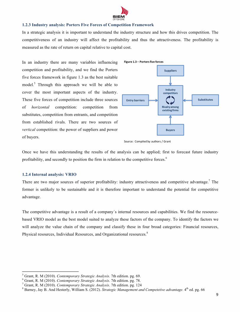
1.2.3 Industry analysis: Porters Five Forces of Competition Framework
In a strategic analysis it is important to understand the industry structure and how this drives competition. The
competitiveness of an industry will affect the profitability and thus the attractiveness. The profitability is
measured as the rate of return on capital relative to capital cost.
In an industry there are many variables influencing
competition and profitability, and we find the Porters
five forces framework in figure 1.3 as the best suitable
model.5 Through this approach we will be able to
cover the most important aspects of the industry.
These five forces of competition include three sources
of horizontal competition: competition from
substitutes, competition from entrants, and competition
from established rivals. There are two sources of
vertical competition: the power of suppliers and power
of buyers.
Once we have this understanding the results of the analysis can be applied; first to forecast future industry
profitability, and secondly to position the firm in relation to the competitive forces.6
1.2.4 Internal analysis: VRIO
There are two major sources of superior profitability: industry attractiveness and competitive advantage.7 The
former is unlikely to be sustainable and it is therefore important to understand the potential for competitive
advantage.
The competitive advantage is a result of a company´s internal resources and capabilities. We find the resource-
based VRIO model as the best model suited to analyze these factors of the company. To identify the factors we
will analyze the value chain of the company and classify these in four broad categories: Financial resources,
Physical resources, Individual Resources, and Organizational resources.8
!!!!!!!!!!!!!!!!!!!!!!!!!!!!!!!!!!!!!!!!!!!!!!!!!!!!!!!!!!!!!5 Grant, R. M (2010). Contemporary Strategic Analysis. 7th edition. pg. 69. 6 Grant, R. M (2010). Contemporary Strategic Analysis. 7th edition. pg. 78. 7 Grant, R. M (2010). Contemporary Strategic Analysis. 7th edition. pg. 124 8 Barney, Jay B. And Hesterly, William S. (2012). Strategic Management and Competetive advantage. 4th ed. pg. 66
Substitutes
Suppliers
Entry barriers
Buyers
Rivalryamongexisting firms
Industry9competitors
Figure 1.39– Porters9five forces
Source:((Compiled by(authors /(Grant(
!!
10!!
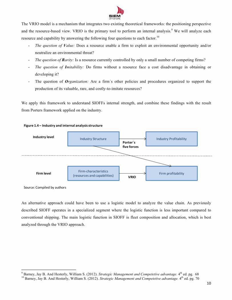
The VRIO model is a mechanism that integrates two existing theoretical frameworks: the positioning perspective
and the resource-based view. VRIO is the primary tool to perform an internal analysis.9 We will analyze each
resource and capability by answering the following four questions to each factor.10
- The question of Value: Does a resource enable a firm to exploit an environmental opportunity and/or
neutralize an environmental threat?
- The question of Rarity: Is a resource currently controlled by only a small number of competing firms?
- The question of Imitability: Do firms without a resource face a cost disadvantage in obtaining or
developing it?
- The question of Organization: Are a firm´s other policies and procedures organized to support the
production of its valuable, rare, and costly-to-imitate resources?
We apply this framework to understand SIOFFs internal strength, and combine these findings with the result
from Porters framework applied on the industry.
An alternative approach could have been to use a logistic model to analyze the value chain. As previously
described SIOFF operates in a specialized segment where the logistic function is less important compared to
conventional shipping. The main logistic function in SIOFF is fleet composition and allocation, which is best
analyzed through the VRIO approach.
!!!!!!!!!!!!!!!!!!!!!!!!!!!!!!!!!!!!!!!!!!!!!!!!!!!!!!!!!!!!!9 Barney, Jay B. And Hesterly, William S. (2012). Strategic Management and Competetive advantage. 4th ed. pg. 68 10 Barney, Jay B. And Hesterly, William S. (2012). Strategic Management and Competetive advantage. 4th ed. pg. 70
Firm%characteristics(resources and capabilities) Firm5profitability
Industry Structure Industry ProfitabilityIndustry)level
Firm)levelVRIO
Porter´sfive forces
Figure 1.4)– Industry)and)internal analysis structure
Source:5Compiled by5authors
!!
11!!
1.2.5 SWOT
SWOT is a framework to understand the internal and external factor influencing SIOFF. The matrix evaluates the
Strength, Weaknesses, Opportunities, and Threats affecting the company. In our thesis we will use the matrix as
a partial conclusion based on our findings in the strategic and financial analysis.
Regression analysis – SAS Enterprise Guide
We have applied a regression analysis to predict future dayrates for the AHTS segment. Based on historical time
series of different explanatory variables, we will run multiple regressions to obtain a linear relationship with our
dependent variable (AHTS dayrates). Description of the model can be seen in appendix 6.1.
Approaches to Valuation
There are numerous approaches to estimate the value of a company. As each approach have different strengths,
weaknesses and limitations, it is necessary to choose a valuation method best suitable for our company.
The choice of model must be based on the inputs available and whether the company is valued as a going
concern. The time available for the analyst will also affect the choice of model, as some models are more time
demanding than others.
The two most common valuation approaches are present value and relative valuation.11 Present value approaches
require a high number of inputs and are considered more labor intensive. As SIOFF is a publicly listed company,
there is plenty of information readily available. We have therefore chosen the Discounted Cash Flow (DCF) and
Economic Value Added (EVA) model, supplemented by a relative valuation to triangulate results. Both the DCF
and EVA model relies on the same input, and will yield the same present value. However the two models provide
different information for how value is created for shareholders.
1.2.6 Discounted Cash Flow Model
Discounted cash flow analysis is the most accurate and flexible method for valuing projects, divisions, and
companies.12 The Discounted cash flow model can be conducted in two ways; either estimate the enterprise value
of a company or estimate the equity value of a company. We have chosen the former. The result from the DCF
model will be the first step in estimating the intrinsic value of SIOFF.
!!!!!!!!!!!!!!!!!!!!!!!!!!!!!!!!!!!!!!!!!!!!!!!!!!!!!!!!!!!!!11 Plenborg & Petersen (2012) – Financial Statement Analysis pg. 210. 12 Koller,T. Goedhart,M. and Wessels,D. (2010) - Valuation: pg. 303
!!
12!!
The value is determined by a forecast of free cash flow to firm (FCFF) in the forecast horizon and terminal
period, which again is discounted by the weighted average cost of capital (WACC). FCFF is calculated by using
the following formula.13
!"!! = !"#$% + !"#$"%&'(&)*! ± !∆!"#! ± ∆!"!!!"##$%&!!"#$"!"%"&' ± ∆!"#$%
Change in non-current liabilities is not considered to be part of NWC or CAPEX, and therefore included as a
separate element. With the estimated FCFF and WACC, we can use the following formula as a two-stage model
to forecast enterprise value:14
!"#$%&%'($!!"#$%! =FCFF!
(1 +WACC)!
!
!!!
+ FCFF!!!(WACC − g)×
1(1 +WACC)!
In order to obtain the estimated market value of equity, we simply deduct the market value of net interesting
bearing debt and the value of minority interests, from our estimated enterprise value.15
1.2.7 Economic Value Added
According to the EVA model the value of a company is determined by the initial invested capital plus the present
value of all future EVAs. The model use the invested capital in the beginning of the period as a starting point for
valuation, and then adds the present value of all future EVAs, which yields the enterprise value of a company.
The EVA is calculated as follows:
!"#! = !"#$%! −!"##×!"#$%&$'!!"#$%"&!!!
We can specify the EVA model in a two-stage formula and calculate the enterprise value of a company.16
!"#$%&%'($!!"#$%! = !"#$%&$'!!"#$%"&! +!"#!
(1 +!"##)!!
!!!+ !"#!!!(!"## − !)×
1(1 +!"##)!
As with the DCF model, we simply deduct market value of net interesting bearing debt and the value of minority
interests.17
!!!!!!!!!!!!!!!!!!!!!!!!!!!!!!!!!!!!!!!!!!!!!!!!!!!!!!!!!!!!!13 Plenborg & Petersen (2012) – Financial Statement Analysis pg. 180 14 Plenborg & Petersen (2012) – Financial Statement Analysis pg. 216 15 Plenborg & Petersen (2012) – Financial Statement Analysis pg.217 16 Plenborg & Petersen (2012) – Financial Statement Analysis pg. 220 17 Plenborg & Petersen (2012) – Financial Statement Analysis pg. 217
!!
13!!
1.2.8 Relative Valuation
Both the DCF and EVA model, however, is only as accurate as the forecasts it relies on. Therefore we have
chosen to perform a relative valuation by using several multiples. By applying this valuation we will test the
plausibility of cash flow forecast and look at how the market prices future sales, revenue and book value of
assets relative to peers. A multiple analysis can yield information for how attractive a company is priced
compared to peers. If a company have a multiple higher than that of peers, it might indicate a higher pricing with
less upside potential. But I can also be a sign of superior market outlook and business prospects. Through this
analysis we will gain input to the discussion of whether SIOFF is a good investment opportunity.
McKinsey mention three requirements in order to carry out a useful analysis of comparable companies.18
1. Use the right multiples
2. Calculate the multiple in a consistent manner
3. Use the right peer group
With regard to the first requirement, there are numerous multiples to choose among. We will present our choice
of multiples in part 8 section 8.3. We have only used forward looking multiples based on current market values,
as there are limited transactions and thus none transaction multiples available.
Multiples for the peer group are obtained from Bloomberg, and are based on an average revenue forecasts from
4-8 investment banks. We will also compare our estimated multiples for SIOFF with market consensus from
Bloomberg. This will provide us with information for the quality of our forecast.
A valuation based on multiples critically relies on the assumption that we find comparable companies with
similar economical characteristic and outlook. A complete overview of the peer group can be seen in appendix
1.2, with an introduction at page 28.
!!!!!!!!!!!!!!!!!!!!!!!!!!!!!!!!!!!!!!!!!!!!!!!!!!!!!!!!!!!!!18 Koller,T. Goedhart,M. and Wessels,D. (2010) - Valuation: pg. 304
!!
14!!
1.2.9 Sensitivity analysis
The output from DCF and EVA model is based on subjective assumptions, and the estimate can therefore be
biased by analysts’ opinion. Some assumptions are more critical than others, and it is important for the investor
to understand how changes in the underlying figure might impact the value of the company.
We have therefore constructed several sensitivity analysis to discuss the most critical assumptions. This process
will illustrate the potential up- or downside as a result of changing market conditions or internal factors.
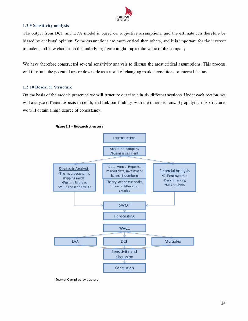
1.2.10 Research Structure
On the basis of the models presented we will structure our thesis in six different sections. Under each section, we
will analyze different aspects in depth, and link our findings with the other sections. By applying this structure,
we will obtain a high degree of consistency.
Introduction
About the.company/business.segment
Theory:.Academic books,.financial litteratur,.
articles
Data:.Annual Reports,.market data,.investment
banks,.Bloomberg
Strategic Analysis•The.macroeconomic.
shipping.model•Porters.5.forces
•Value chain and.VRIO
Forecasting
Financial.Analysis•DuPont.pyramid•Benchmarking•Risk Analysis
SWOT
WACC
EVA DCF
Sensitivity and.discussion
Conclusion
Multiples
Figure 1.5*– Research*structure
Source:.Compiled by.authors
!!
15!!
1.3 Delimitation ' As SIOFF is a publicly listed company, we have only used publicly available information.
' Our benchmark for SIOFFs shareprice is set to 16th of April 2013, as this is the date the annual report from
2012 was publicly available. Any information after this date has not been taken into consideration.
' In some of the analysis we have only used four years of historical data, as a result of lack of segregation in
the annual report.
' Some vessels have contracts which can be extended by charterer. There is great uncertainty if these options
will be exercised. We have assumed that options will be renegotiated at market terms, which will reflect our
forecast for spot rates. Options will therefore not affect the final output.
' The gas price is closely correlated with the oil price in all markets except from US. We have therefore only
forecasted the oil price as we expect the gas price to follow closely.
' We have not activated operational leasing as it would not impact the final output due to insignificance.
' SIOFF has operations in a business segment called Scientific Core Drilling. This segment consists of one
very old vessel (JOIDES Resolution), and not considered as core business. We have therefore excluded this
vessel from our analysis to value SIOFF core operations.
' The well intervention vessel (Big Orange XVIII) is part of income from associated companies.
' The FSV, FCV and OSRV in Brazil are on long term contracts with fixed rates. We have therefore not
analyzed this segment in depth. The very old vessels are assumed scrapped end of 2012, as all the new
FSV/FCV vessels now are delivered.
' Siem WIS is owned 60% by SIOFF, and is a venture company within the area of drilling pressure
technology. As this is neither core operations nor have historical revenue of significance, we have excluded
this associated company from our analysis, and estimated the market value to NOK 0.
!
!!
16!!
2.0 Introduction to Siem Offshore and the offshore supply vessel (OSV) industry 2.1 Siem Offshore Inc. Siem Offshore Inc. is one of the fastest growing Norwegian offshore supply companies (OSV), offering marine
services to the offshore oil and gas industry worldwide.19 The company was established in July 2005 following a
spin-off from the company Subsea 7 Inc. The customers are primarily upstream petroleum companies and Siem
provides a broad specter of services such as movement of marine equipment, supply to offshore installations and
various range of subsea construction support. These tasks are performed trough the management and ownership
of 33 vessels and 1078 employees, of which 250 are employed onshore and 828 are employed on vessels.20 The
headquarter is located in Kristiansand, Norway, and the company is listed at the Oslo Stock Exchange under the
ticker SIOFF. The current market cap is NOK 2.85bn and the total operating revenue for 2012 was USD 310
million. Before we go on and describe SIOFF further, we will first present the OSV market where SIOFF
operates.
2.2 The offshore supply market (OSV) The offshore supply market is a highly fragmented market with 95 companies controlling a fleet of 10 vessels or
more. There are few dominant players, and none of the companies have any particular pricing power.21 With an
efficient organization, technical competence and fleet quality the companies can affect the utilization of the
vessels. Higher utilization is equal to greater revenue potential.
While onshore petroleum production can be a fairly simple business, offshore production is highly demanding
and operationally challenging. The operator needs to address challenges such as extreme weather conditions,
ultra deep water, advanced technology, long distances and high operational risks.22 The demand for OSV vessels
can therefore best be described by the value chain for the petroleum industry:
!!!!!!!!!!!!!!!!!!!!!!!!!!!!!!!!!!!!!!!!!!!!!!!!!!!!!!!!!!!!!19 Siem Offshore – Annual report (2012) pg. 7 20 Siem Offshore - Annual report (2012) pg.9 21 ABG Sundal Collier – Offshore Supply – Sector initiation (10.04.2013) pg. 10 22 The Macondo accident in Gulf of Mexico is one example of this risk.
!!
17!!
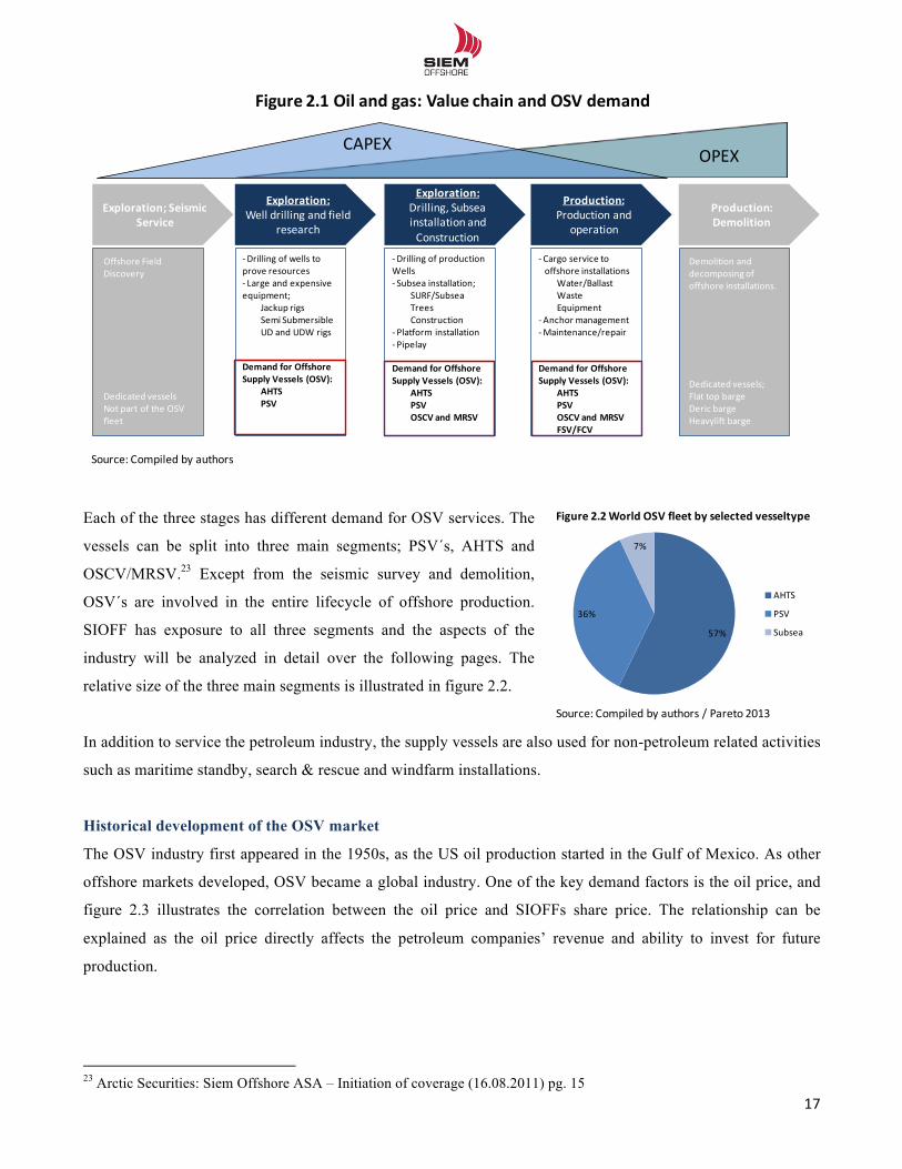
Each of the three stages has different demand for OSV services. The
vessels can be split into three main segments; PSV´s, AHTS and
OSCV/MRSV.23 Except from the seismic survey and demolition,
OSV´s are involved in the entire lifecycle of offshore production.
SIOFF has exposure to all three segments and the aspects of the
industry will be analyzed in detail over the following pages. The
relative size of the three main segments is illustrated in figure 2.2.
In addition to service the petroleum industry, the supply vessels are also used for non-petroleum related activities
such as maritime standby, search & rescue and windfarm installations.
Historical development of the OSV market
The OSV industry first appeared in the 1950s, as the US oil production started in the Gulf of Mexico. As other
offshore markets developed, OSV became a global industry. One of the key demand factors is the oil price, and
figure 2.3 illustrates the correlation between the oil price and SIOFFs share price. The relationship can be
explained as the oil price directly affects the petroleum companies’ revenue and ability to invest for future
production.
!!!!!!!!!!!!!!!!!!!!!!!!!!!!!!!!!!!!!!!!!!!!!!!!!!!!!!!!!!!!!23 Arctic Securities: Siem Offshore ASA – Initiation of coverage (16.08.2011) pg. 15
Exploration;,SeismicService
OPEX
Offshore+FieldDiscovery
Dedicated vesselsNot+part+of+the+OSVfleet
Exploration:,Well drilling and+field
research
=Drilling of+wells toprove resources= Large+and+expensiveequipment;
Jackup rigsSemi SubmersibleUD+and+UDW+rigs
Demand for,OffshoreSupply Vessels,(OSV):
AHTSPSV
Exploration:Drilling,+Subseainstallation+and+Construction
=Drilling of+productionWells= Subsea installation;
SURF/SubseaTreesConstruction
= Platform+installation= Pipelay
Demand for,OffshoreSupply Vessels,(OSV):
AHTSPSVOSCV,and,MRSV
Production:,Production and+
operation
= Cargo service+tooffshore+installations
Water/BallastWasteEquipment
= Anchor management=Maintenance/repair
Demand for,OffshoreSupply Vessels,(OSV):
AHTSPSVOSCV,and,MRSVFSV/FCV
Production:Demolition
Figure 2.1,Oil,and,gas:,Value chain and,OSV,demand
CAPEX
Source:+Compiled by+authors
Demolition and+decomposing of+offshore+installations.
Dedicated vessels;Flat top+bargeDeric bargeHeavylift barge
57%
36%
7%
AHTS
PSV
Subsea
Source:5Compiled by5authors /5Pareto 2013
Figure 2.2)World)OSV)fleet by)selected vesseltype
!!
18!!
Their E&P spending directly affect the demand for OSV`s, as can be seen from the first stages in figure 2.1. The
cost associated with petroleum production is tremendous and the companies therefore monitor the price trends
closely.
During the period from 2005 – 2008 the oil price reached levels never previously seen. Offshore investments
reached an all time high, and OSV dayrates were booming. As there are few dominant participants, vessel
owners reacted independently, vigorously ordering new tonnage.24
In 2008 the financial crises evolved and the oil price plunged. As a reaction, the petroleum companies nominal
growth in E&P spending turned negative, removing half the OSV demand.25 Other offshore projects were also
postponed or cancelled, affecting the submarine cable and renewable energy business.
In 2009 the global economy showed signs of improvement, but as more and more of the newbuildings were
delivered, a huge imbalance occurred between supply and demand.26 Since then, overhang of tonnage has
dominated the development in the OSV industry, which can explain the weakened relationship between the oil
price and SIOFF´s share price. Today the demand has turned more towards the high-end segment of both the
AHTS and PSV market, where SIOFF has its main exposure.27
!!!!!!!!!!!!!!!!!!!!!!!!!!!!!!!!!!!!!!!!!!!!!!!!!!!!!!!!!!!!!24 RS Platou Market – The Platou Report June (2008) pg. 10 25 Pareto Securities: Supply Research report (19.09.2011) pg. 1 26 Siem Offshore – Annual Report (2009) pg. 11. 27 Arctic Securities: Offshore Supply – Sector initiation (10.04.2013) pg. 57
Source:(Compiledby(authors /(Oslo(Børs((/(FRED(Data
0
20
40
60
80
100
120
140
160
0
5
10
15
20
25
2005 2006 2007 2008 2009 2010 2011 2012
Figure'2.3'Oilprice'development'vs.'SIOFF'share
Shareprice Oilprice((brent(3m)
USD/bblNOK
!!
19!!
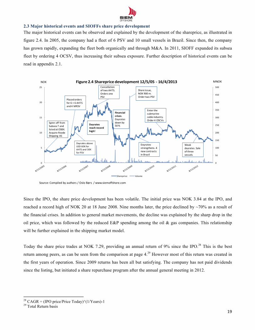
2.3 Major historical events and SIOFFs share price development The major historical events can be observed and explained by the development of the shareprice, as illustrated in
figure 2.4. In 2005, the company had a fleet of 6 PSV and 10 small vessels in Brazil. Since then, the company
has grown rapidly, expanding the fleet both organically and through M&A. In 2011, SIOFF expanded its subsea
fleet by ordering 4 OCSV, thus increasing their subsea exposure. Further description of historical events can be
read in appendix 2.1.
Since the IPO, the share price development has been volatile. The initial price was NOK 3.84 at the IPO, and
reached a record high of NOK 20 at 18 June 2008. Nine months later, the price declined by ~70% as a result of
the financial crises. In addition to general market movements, the decline was explained by the sharp drop in the
oil price, which was followed by the reduced E&P spending among the oil & gas companies. This relationship
will be further explained in the shipping market model.
Today the share price trades at NOK 7.29, providing an annual return of 9% since the IPO.28 This is the best
return among peers, as can be seen from the comparison at page 4.29 However most of this return was created in
the first years of operation. Since 2009 returns has been all but satisfying. The company has not paid dividends
since the listing, but initiated a share repurchase program after the annual general meeting in 2012.
!!!!!!!!!!!!!!!!!!!!!!!!!!!!!!!!!!!!!!!!!!!!!!!!!!!!!!!!!!!!!28 CAGR = (IPO price/Price Today)^(1/Years)-1 29 Total Return basis
0
50
100
150
200
250
300
350
400
450
500
0
5
10
15
20
25
Figure'2.4'Shareprice'development'12/5/05'; 16/4/2013
Shareprice Volume
Spinn off from6Subsea 76and6listedat6OSBX.6Acquire RovdeShipping6AS
Placedordersfor666+666AHTS6and646MRSV
Dayrates6aboveUSD660K6for6AHTS6and630K6for6PSV
Cancellationof6two AHTS.6Orders onePSV
Financial'crises.6Dayrates6down by6506%
Share issue,6NOK69006m.6Order two PSV
Dayrates6strengthens.646new6contractsin6Brazil
Enter the6submarine6cable industry.6Order 46OSCVs
Weakdayrates.6Sale6of6threevessels
Dayrates'reach recordhigh!
NOK MNOK
Source:6Compiled by6authors /6Oslo6Børs66/6www.siemoffshore.com
!!
20!!
2.4 Organization SIOFF is a fully integrated OSV company, in terms of both ownership and operations. The company´s operation
is mainly run from Norway, with additional offices in Germany, the Netherlands and India. The fleet is located in
the North Sea, South America and West Africa. The Brazilian fleet is managed and operated through Siem
Consub, a fully owned Brazilian subsidiary. The remaining subsidiaries have little organizational importance
except from dispersing of the ownership of the vessels. There are also some minority interests, regard four of the
PSVs. The whole organizational structure can be seen from
appendix 2.2
Objectives, strategy and business concept
In order for a company to achieve its goals and create value for the owners, it needs a clear strategy with outlined
objectives. In a valuation perspective it is therefore important to understand SIOFFs objectives and business
concept. Through the thesis we will analyze the business internally and externally, and evaluate how successful
SIOFFs strategy has been.30
• Siem Offshore aims to grow the company within offshore support vessels, both organically and through
combination with other operators, in order to achieve economies of scale and stronger presence in the
market.
• Siem Offshore aims to become a preferred supplier of marine services to the oil & gas industries based
on quality and reliability and provide cost efficient solutions for its customers by understanding their
operation and applying technology and experience.
• The Company builds its business around a motivated workforce with the appropriate technical solutions
and creating sustainable value to all shareholders.
!
!
!
!
!
!
!
!!!!!!!!!!!!!!!!!!!!!!!!!!!!!!!!!!!!!!!!!!!!!!!!!!!!!!!!!!!!!30 www.siemoffshore.com – Investor relations – Corporate governance
!!
21!!
2.5 Management team and board of directors The management team of SIOFF consists of five members, all Norwegian citizens.31 None of the members have
familiar ties to the largest owners.
CEO – Terje Sørensen (born 1964)
Mr. Sørensen was appointed CEO in 2005, thus SIOFF has only had one CEO during the eight years of
operations. He came from the position as CFO for Siem Offshore Inc. with prior experience from various
companies such as Mosvold Shipping AS and Norsk Skibs Hypotekbank AS. Mr. Terje Sørensen, holds
1.900.000 shares in SIOFF, ~0.48 % of outstanding shares.32
CFO – Dagfinn B. Lie (born 1972)
Mr. Lie is the youngest member of the management team and has been SIOFFs CFO since 2009. He holds an
MBA for the Norwegian School of Business and has gained experience from companies such as Wallenius
Wilhelmsen Logistics and ABB Offshore.
COO – Svein Erik Mykland (born 1966)
Prior to his promotion to COO in 2010, Mr. Mykland was employed as AHTS director in SIOFF since 2008. For
the last 25 years, Mr. Mykland has been employed in the offshore industry and has a broad experience from both
onshore and offshore operations. He was originally recruited from Acergy (Subsea Constructors) where he held
the position as Group Operation Manager.
In addition to those mentioned, Mr. Bernt Omdal is employed as Chartering Director and Mr. Tore Johannessen
is employed as Global HR Director.
Board of directors
The board of directors consists of five men, where two are Norwegian citizens. Mr. Eystein Eriksrud is the
chairman and is also the Deputy CEO of Siem Industries Inc., SIOFFs main shareholder. Mr. Kristian Siem is the
owner of Siem Industries, and is also represented as Board Member for SIOFF. The other members of the board
are Mr. Michael Delouche (U.S.), Mr. David Mullen (Ireland) and Mr. John C. Wallace (Canada).
!!!!!!!!!!!!!!!!!!!!!!!!!!!!!!!!!!!!!!!!!!!!!!!!!!!!!!!!!!!!!31 www.siemoffshore.com – Company – Management Team 32 Siem Offshore – Annual Report (2012) pg. 91
!!
22!!
2.6 Ownership structure While many of the Norwegian offshore companies are dominated by
family ownership, SIOFF is controlled by an individual private
investor.33 The 20 largest shareholders control more than 76 % of
the shares outstanding, and the top 5 shareholders owns ~60 %.
The dominating shareholder is Siem Industries Inc. with ~34 % of
the ownership. Over 70 % of the shares in this company is owned
and controlled by the Norwegian investor Kristian Siem and his
family. The second largest shareholder is Ace Crown International Ltd., an investor group based outside
European legislations. The remaining shares are spread among mostly Norwegian trusts and funds.34 The average
trading volume is between NOK 0.5 – 1 mill per day.35
2.7 The SIOFF fleet and business areas The SIOFF fleet counts a total number of 33 operating vessels plus 10 newbuilds with delivery in the upcoming
two years, as can be seen in table 2.1. This newbuilding program represents more than USD 2.3 bn. in
investments.36 Since the spinoff from Subsea 7 the fleet growth has been remarkable. Over the years the fleet has
grown by more than 20 vessels. Today the fleet is the youngest among peers, with average age of 3-4 years.37
The entire fleet list can be seen in appendix 2.3.
!!!!!!!!!!!!!!!!!!!!!!!!!!!!!!!!!!!!!!!!!!!!!!!!!!!!!!!!!!!!!33 Family ownership; DOF (55 %), Farstad (60%) Havila (55%) Solstad Offshore (45%)SIOFF (36%)Eidesvik (67%) 34 Siem Offshore – Annual Report (2012) pg. 91. 35 Datastream - SIOFF 36 Siem Offshore ASA – Company presentations, Pareto conference (12.08.2012), pg. 2 37 Siem Offshore ASA – Company presentations, Pareto conference (12.08.2012), pg. 2
Table&2.1Vessel&type Number Newbuilds
PSV>900m2 4 3<900m2 7
AHTS>25.000 8
SubseaOSCV 4MRSV 2Other 1 1
Brazilian&fleetFCV 2FSV 7OSRV 2 2
Scientific&Drilling 33 10Source:8Compiled8by8authors8/8SIOFF8AR82012
33.66%
19.39%
2.69%2.30%2.27%
39.69%
Figure'2.5.'Ownership'structure
Siem.Industries.Inc.
Ace.Crown.International.Ltd.
Verdipapirfondet.Handelsbanken
MP.Pensjon.PK
Skagen.KonITiki
Other
Source:.Compiled by.authors /.Annual Report 2012
!!
23!!
As can be seen from the figure 2.6, SIOFF has operations within
four different business areas. The core business is the operation of
OSV vessels, in the AHTS, PSV and subsea segment. In 2012 this
accounted for 85% of EBITDA.38 The Brazilian vessels are small
cargo/personnel carriers and have limited contribution to the
result. Sale of vessels has fluctuated between USD -8 and 13
million and is treated as a result of core operation. While asset
plays is common for traditional shipping segments, it is not usual
for OSV companies to practice this. Sale of vessels is therefore
not likely to account for as much as 11% of EBITDA in the
future.
2.7.1 The AHTS segment (Anchor-Handler-Tug-Supply)
The AHTS vessels are specifically designed for the purpose of towing and anchoring offshore installations, such
as Jackup rigs, semi rigs and floating production units (FPSO). This equipment is of high value and can weigh
several hundred tons. The largest AHTS vessels are therefore fitted with engines up to 35.000 bhp. A recent
trend is that UDW39 rigs are equipped with DP (Dynamical Positioning).40 This can possibly reduce demand for
AHTS, since the rigs are capable of transporting and positioning themselves. Despite this, UDW rigs might still
demand service from AHTS vessels when drilling in shallow water, for long distance transportation and when
drilling at the same field for longer period of time.41 As installations and equipment has become larger, the
demand has shifted more towards the high-end segment.42
!!!!!!!!!!!!!!!!!!!!!!!!!!!!!!!!!!!!!!!!!!!!!!!!!!!!!!!!!!!!!38 Siem Offshore – Annual report (2012) pg. 58 39 Ultra Deep Water 40 DP is a system that allow for the rigs to maneuver themselves 41 Arctic: Siem Offshore ASA – Initiation of coverage (16.08.2011) pg. 15 42 Characterized as more than 20.000 Bhp.
Picture(1.1(AHTS(Vessel
Source:(www.siemoffshore.com
Source:(Compiled by(authors /(Annual Report
PSV29%
MRSV/(OSCV19%
AHTS37%
FSV/FCV4%
Sale(of(vessels11%
EBITDA'contribution'pr.'business'segment'2012
!!
24!!
As can be seen from the table 2.1, SIOFF owns 8 AHTS vessels. The whole AHTS fleet is built in Norway and
with its 28.000 bhp. we classify the fleet as being high-end. The average fleet age is three years and the
newbuilding price is USD 88m today. Over the last 10 years average quarterly dayrates have fluctuated between
NOK 200 and 600k.
2.7.2 The PSV segment (Platform Supply Vessel)
PSVs are the “work horse” of the ocean and were among the first vessels developed for serving the petroleum
industry. The vessels are designed for transportation of various supplies to and from the variety of offshore
installations. Therefore the vessels are equipped with large tanks to contain water, ballast and fuel, and large
deckspace for pipes, hauling risers and waste.43 Compared to the AHTS vessels, the design is simple and the
complexity is correspondingly lower. The demand-trend is the same as for AHTS, with increasingly focus on
high-end vessels with large deckspace. PSVs are classified by cargo deck area (CDA), where high-end is above
900m2.44
SIOFF has currently a fleet of 11 PSVs with an additional three for delivery in 2013/2014. Two of these are
under construction in Brazil. The majority of the fleet is built in Norway and is classified as large size/high-end.
But SIOFF has also exposure towards the mid size segment with a total of 6 vessels.
!!!!!!!!!!!!!!!!!!!!!!!!!!!!!!!!!!!!!!!!!!!!!!!!!!!!!!!!!!!!!43 Arctic Securities: Siem Offshore ASA – Initiation of coverage (16.08.2011) pg. 15 44 The Platou Report (2013) pg. 37
Picture(1.2(PSV(Vessel
Source:(www.siemoffshore.com
!!
25!!
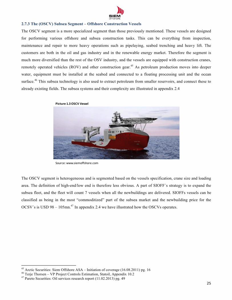
2.7.3 The (OSCV) Subsea Segment – Offshore Construction Vessels
The OSCV segment is a more specialized segment than those previously mentioned. These vessels are designed
for performing various offshore and subsea construction tasks. This can be everything from inspection,
maintenance and repair to more heavy operations such as pipelaying, seabed trenching and heavy lift. The
customers are both in the oil and gas industry and in the renewable energy market. Therefore the segment is
much more diversified than the rest of the OSV industry, and the vessels are equipped with construction cranes,
remotely operated vehicles (ROV) and other construction gear.45 As petroleum production moves into deeper
water, equipment must be installed at the seabed and connected to a floating processing unit and the ocean
surface.46 This subsea technology is also used to extract petroleum from smaller reservoirs, and connect these to
already existing fields. The subsea systems and their complexity are illustrated in appendix 2.4
The OSCV segment is heterogeneous and is segmented based on the vessels specification, crane size and loading
area. The definition of high-end/low end is therefore less obvious. A part of SIOFF´s strategy is to expand the
subsea fleet, and the fleet will count 7 vessels when all the newbuildings are delivered. SIOFFs vessels can be
classified as being in the most “commoditized” part of the subsea market and the newbuilding price for the
OCSV´s is USD 98 – 105mn.47 In appendix 2.4 we have illustrated how the OSCVs operates.
!!!!!!!!!!!!!!!!!!!!!!!!!!!!!!!!!!!!!!!!!!!!!!!!!!!!!!!!!!!!!45 Arctic Securities: Siem Offshore ASA – Initiation of coverage (16.08.2011) pg. 16 46 Terje Thorsen – VP Project Controls Estimation, Statoil, Appendix 10.2 47 Pareto Securities: Oil services research report (11.02.2013) pg. 49
Picture(1.3(OSCV(Vessel
Source:(www.siemoffshore.com
!!
26!!
The FSV (Fast Supply vessels), FCV (Fast Crew Vessels) and the OSRV (Oil Spill Recovery Vessels)
As can be seen from table 2.1, the Brazilian fleet counts 11 vessels plus two newbuildings. FSVs and FCVs are
specialized for high speed passenger and light cargo transportation, and are easy to both build and operate. The
newbuilding price is only USD 5 – 10 m, and the dayrates are correspondingly lower compared to the other OSV
segments.48 The OSRVs are standby vessels in case of offshore accidents. All these vessels are on long term
contract with the Brazilian company Petrobras. The FCV/FSV vessels were delivered in 2011/12 and replaced
older vessels. Two OSRVS will be delivered mid 2013.
Siem Offshore Contractors - SOC
Siem Offshore Contractors was owned 50% by SIOFF until 2011 when the remaining 50% was acquired. SOC is
a submarine cable contractor and through this business area, SIOFF provides cable and umbilical installation,
repair and maintenance services. The company is managed as a subdivision and provides service to both the
renewable and petroleum sector. By utilizing in-house resources such as PSV, AHTS and Subsea vessels, SOC
can install, maintain and repair submarine cables as well as subsea umbilical in any water depths and
geographical area.49 In 2014 SIOFF will take delivery of one ISV (Installation Support Vessel) to support the
renewable business. The CAPEX for this vessel is approximately USD 52.5 m.50 The Company has a order
backlog of USD 180m over the next two years.51
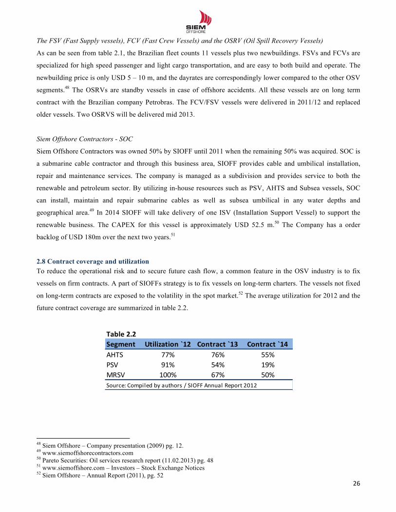
2.8 Contract coverage and utilization To reduce the operational risk and to secure future cash flow, a common feature in the OSV industry is to fix
vessels on firm contracts. A part of SIOFFs strategy is to fix vessels on long-term charters. The vessels not fixed
on long-term contracts are exposed to the volatility in the spot market.52 The average utilization for 2012 and the
future contract coverage are summarized in table 2.2.
!!!!!!!!!!!!!!!!!!!!!!!!!!!!!!!!!!!!!!!!!!!!!!!!!!!!!!!!!!!!!48 Siem Offshore – Company presentation (2009) pg. 12. 49 www.siemoffshorecontractors.com 50 Pareto Securities: Oil services research report (11.02.2013) pg. 48 51 www.siemoffshore.com – Investors – Stock Exchange Notices 52 Siem Offshore – Annual Report (2011), pg. 52
Table&2.2Segment Utilization&`12 Contract&`13 Contract&`14AHTS 77% 76% 55%PSV 91% 54% 19%MRSV 100% 67% 50%Source:7Compiled7by7authors7/7SIOFF7Annual7Report72012
!!
27!!
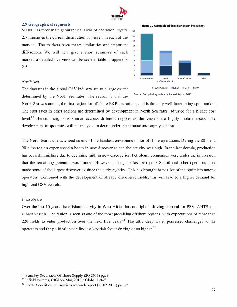
2.9 Geographical segments SIOFF has three main geographical areas of operation. Figure
2.7 illustrates the current distribution of vessels in each of the
markets. The markets have many similarities and important
differences. We will here give a short summary of each
market, a detailed overview can be seen in table in appendix
2.5.
North Sea
The dayrates in the global OSV industry are to a large extent
determined by the North Sea rates. The reason is that the
North Sea was among the first region for offshore E&P operations, and is the only well functioning spot market.
The spot rates in other regions are determined by development in North Sea rates, adjusted for a higher cost
level.53 Hence, margins is similar accross different regions as the vessels are highly mobile assets. The
development in spot rates will be analyzed in detail under the demand and supply section.
The North Sea is characterized as one of the harshest environments for offshore operations. During the 80`s and
90`s the region experienced a boom in new discoveries and the activity was high. In the last decade, production
has been diminishing due to declining faith in new discoveries. Petroleum companies were under the impression
that the remaining potential was limited. However, during the last two years Statoil and other operators have
made some of the largest discoveries since the early eighties. This has brought back a lot of the optimism among
operators. Combined with the development of already discovered fields, this will lead to a higher demand for
high-end OSV vessels.
West Africa
Over the last 10 years the offshore activity in West Africa has multiplied, driving demand for PSV, AHTS and
subsea vessels. The region is seen as one of the most promising offshore regions, with expectations of more than
220 fields to enter production over the next five years.54 The ultra deep water possesses challenges to the
operators and the political instability is a key risk factor driving costs higher.55
!!!!!!!!!!!!!!!!!!!!!!!!!!!!!!!!!!!!!!!!!!!!!!!!!!!!!!!!!!!!!53 Fearnley Securities: Offshore Supply (2Q 2011) pg. 9 54 Infield systems, Offshore Mag 2012, “Global Data” 55 Pareto Securities: Oil services research report (11.02.2013) pg. 39
Source:(Compiled by(authors /(Annual Report 2012
0
2
4
6
8
10
12
14
16
18
America/Brazil North(Sea/Norwegian(Sea
Africa/Guinea Other
Figure'2.7'Geographical'fleet'distribution'by'segment
FSV/FCV/OSRV MRSV AHTS PSV
!!
28!!
South America
Brazil has over the last decade become one of the world´s leading petroleum regions with growth in reserves of
more than 68.5%.56 The fields are located far from shore (three times as far compared to North Sea) in some of
the world`s greatest water depths. This requires larger rigs for complex operations, as well as higher demand for
subsea installations.57
Although Brazil is a high growth market with opportunities for OSV players, it’s a difficult market to operate.
Brazil has internal challenges in terms of bureaucracy, corruption and requirements for local content. In order to
protect national interest the Government has adopted strict regulations that require vessels to be Brazilian built
and staffed with Brazilian crew. Vessels built in other countries can enter the market only after paying
government import tax. This has created problems of cost inflation, particularly due to the tight supply of labor.
2.10 Definition of peer group The purpose of defining a peer group is to analyze SIOFF´s relative performance over an historical period. The
peer group will be used as a benchmark in the strategic- and financial analysis, in addition to the relative
valuation (multiples).
A peer group does not necessarily need to comprise of competitors, but there are several consideration that must
be taken in consideration. Most importantly the firms need to be comparable in terms of operation and business
characteristics, and the financial statements must be based upon the same accounting principles.58 The risk
profile in the peer group should also be alike, and for the use of multiples, peers should have similar outlook for
long term growth and return on capital (ROIC).59
As previously described, the OSV industry is a highly fragmented shipping segment with hundreds of vessel
owners. Of practical considerations it is therefore impossible to identify the specific competitors, as they differ in
each market. The selection of a Norwegian peer group was eventually natural as Norwegian owners have the
most comparable fleet, typically classified within the medium- to high-end segment. They also have operations
in many of the same geographical markets, and are thus competing for the same employment. By comparing
companies in the same industry with similar characteristics, we will secure appropriate relevance of financial
ratios.60 An alternative could have been to look at companies in other industries, with similar organizational
structure, value chain or financial performance. As the OSV industry is a specialized market, we find it more
advantageous to benchmark towards other industry peers.
!!!!!!!!!!!!!!!!!!!!!!!!!!!!!!!!!!!!!!!!!!!!!!!!!!!!!!!!!!!!!56 DOF ASA – Annual Report (2011) pg. 19 57 Terje Thorsen, VP Project Controls Estimation, Statoil Appendix 10.2 58 Plenborg & Petersen (2012) – Financial Statement Analysis pg. 64 59 Koller,T. Goedhart,M. and Wessels,D. (2010) - Valuation: pg. 305 60 Plenborg & Petersen (2012) – Financial Statement Analysis pg. 65
!!
29!!
To determine the peer group we have performed a comparison of the eight OSV companies listed at Oslo Stock
Exchange. The companies have been ranked based on operational criteria´s and the comparison can be seen in
appendix 1.2. Based on the peer group analysis, the following companies have been chosen; DOF ASA, Farstad
Shipping ASA, Solstad Offshore ASA and Havila Shipping ASA.
Although there are similarities among peers, we acknowledge the individual differences. Most importantly
Farstad Shipping has a strong presence in the Indian Pacific and DOF has more than 70 % of its revenue from the
Subsea segment. Despite of this we see the peer group as the most acceptable comparable firms as they have
similar organizational structure and comparable value chain. This is confirmed by industry analysts.61 A short
presentation of the companies in the peer group will be given in the following section:
DOF ASA
DOF is the largest Norwegian OSV company with a total of 74 vessels.62 This includes 7 newbuildings. Over the
last five years DOF has been the most aggressive player in terms of vessel orders, and as a consequence of this
the company is heavy leveraged.63 DOF has traditionally had a high degree of contract coverage and the main
area of operation is the North Sea, Brazil and Indian Pacific. 64 In 2012 the company had a total operating income
of NOK 8.1bn. and employed more than 4.000 people. Contract coverage for 2013 is 81%.
Farstad Shipping ASA
Farstad is the second largest of the Norwegian players with 57 vessels and 7 newbuilds.65 The last year’s fleet
growth has been funded through operational cash flow, equity and debt, making the balance sheet particularly
strong compared to the industry. The company is recognized as a “blue chip” company with historical industry
leading returns.66 Farstad has a strong presence in Brazil through a wholly owned subsidiary. Other areas of
operation include North Sea, Gulf of Mexico Indian Pacific. The total operating income for 2012 was NOK
3.7bn. and the company employed more than 2.000 people. Contract coverage for 2013 is 65%.
!!!!!!!!!!!!!!!!!!!!!!!!!!!!!!!!!!!!!!!!!!!!!!!!!!!!!!!!!!!!!61 Arctic Securities, Pareto Securities, First Securities. 62 DOF ASA – (Q3 2012) pg. 4 63 Pareto Securities: Oil services research report (11.02.2013) pg. 121 64 DOF ASA – (Q3 2012) pg. 4 65 Farstad Shipping – (Q4 2012) pg. 3. 66 Pareto Securities: Oil services research report (11.02.2013) pg. 112
!!
30!!
Solstad Offshore ASA
Solstad is a strong global player in the OSV market with operations in North Sea, Africa, Gulf of Mexico, Brazil
and Asia Pacific. The fleet counts a total of 50 vessels plus one newbuilding. Over the last years Solstad has
expanded the fleet of subsea vessels and are increasing its focus on this segment.67 In 2012 the total operating
income was NOK 3.4bn and the company employed around 1400 people. Contract coverage for 2013 is 78%.
Havila Shipping ASA
Havila was listed at Oslo Stock Exchange in 2005, the same year as SIOFF. The company operates a fleet of 28
vessels where four are owned by a joint venture and one is leased. Over the last years the company has grown the
fleet tremendously and as a result the company is highly leveraged with high cost of debt. The company follows
a strategy with high contract coverage, but is currently running 6-8 vessels in the spot market.68 The total
operating income in 2012 was NOK 1.4bn. and the total employment is approximately 600. Contract coverage
for 2013 is 81%
The shareprice development of the peer group can be seen in figure 1.1 pg. 4 in the introduction.
!
!
!
!
!
!!!!!!!!!!!!!!!!!!!!!!!!!!!!!!!!!!!!!!!!!!!!!!!!!!!!!!!!!!!!!67 Pareto Securities: Oil services research report (11.02.2013) pg. 117 68 Pareto Securities: Oil services research report (11.02.2013) pg. 134
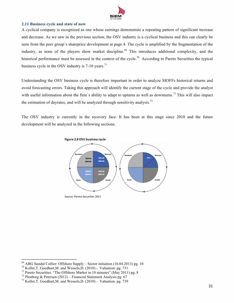
!!
31!!
2.11 Business cycle and state of now A cyclical company is recognized as one whose earnings demonstrate a repeating pattern of significant increase
and decrease. As we saw in the previous section, the OSV industry is a cyclical business and this can clearly be
seen from the peer group´s shareprice development at page 4. The cycle is amplified by the fragmentation of the
industry, as none of the players show market discipline.69 This introduces additional complexity, and the
historical performance must be assessed in the context of the cycle.70 According to Pareto Securities the typical
business cycle in the OSV industry is 7-10 years.71
Understanding the OSV business cycle is therefore important in order to analyze SIOFFs historical returns and
avoid forecasting errors. Taking this approach will identify the current stage of the cycle and provide the analyst
with useful information about the firm´s ability to adapt to upturns as well as downturns.72 This will also impact
the estimation of dayrates, and will be analyzed through sensitivity analysis.73
The OSV industry is currently in the recovery face. It has been at this stage since 2010 and the future
development will be analyzed in the following sections.
!
!!!!!!!!!!!!!!!!!!!!!!!!!!!!!!!!!!!!!!!!!!!!!!!!!!!!!!!!!!!!!69 ABG Sundal Collier: Offshore Supply – Sector initiation (10.04.2013) pg. 10 70 Koller,T. Goedhart,M. and Wessels,D. (2010) - Valuation: pg. 731 71 Pareto Securities: “The Offshore Market in 10 minutes” (May 2011) pg. 8 72 Plenborg & Petersen (2012) – Financial Statement Analysis pg. 67 73 Koller,T. Goedhart,M. and Wessels,D. (2010) - Valuation: pg. 739
Source:(Pareto Securities 2011
Figure 2.8*OSV*business*cycle
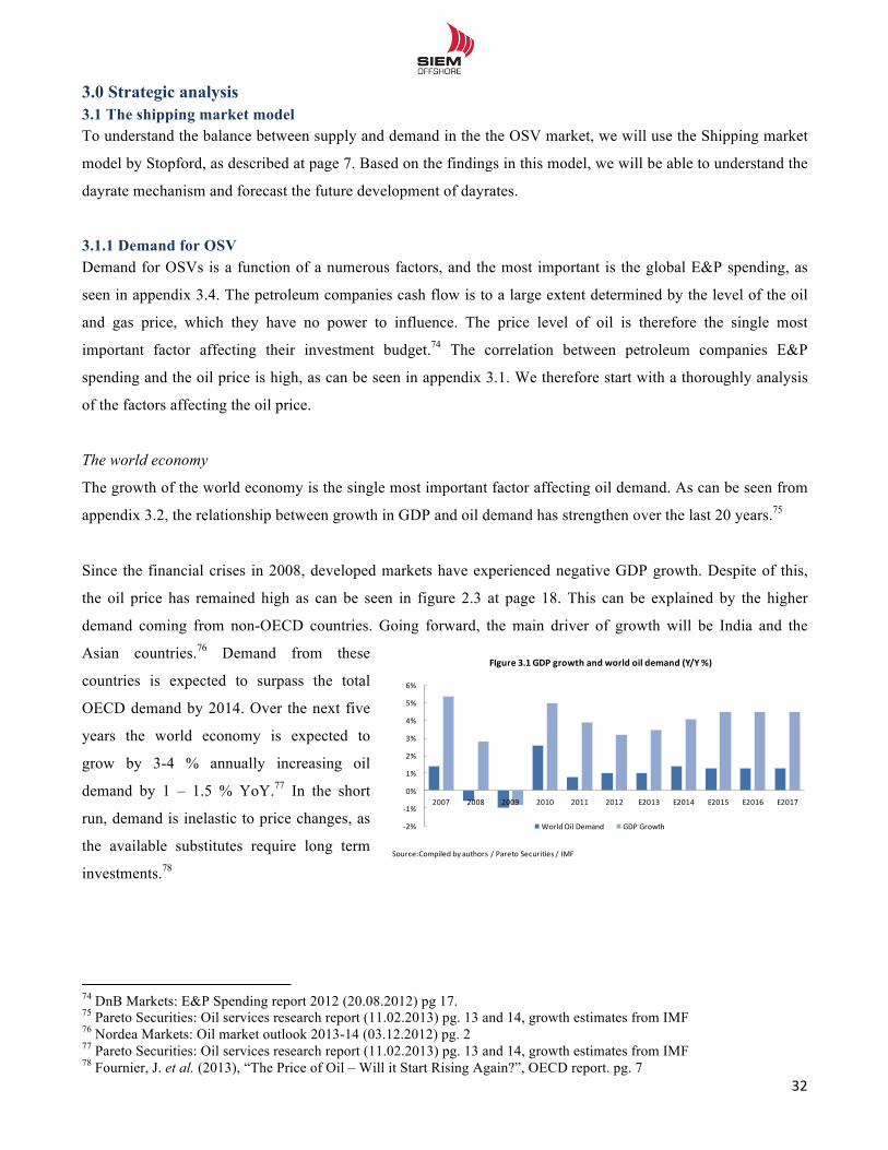
!!
32!!
3.0 Strategic analysis 3.1 The shipping market model To understand the balance between supply and demand in the the OSV market, we will use the Shipping market
model by Stopford, as described at page 7. Based on the findings in this model, we will be able to understand the
dayrate mechanism and forecast the future development of dayrates.
3.1.1 Demand for OSV Demand for OSVs is a function of a numerous factors, and the most important is the global E&P spending, as
seen in appendix 3.4. The petroleum companies cash flow is to a large extent determined by the level of the oil
and gas price, which they have no power to influence. The price level of oil is therefore the single most
important factor affecting their investment budget.74 The correlation between petroleum companies E&P
spending and the oil price is high, as can be seen in appendix 3.1. We therefore start with a thoroughly analysis
of the factors affecting the oil price.
The world economy
The growth of the world economy is the single most important factor affecting oil demand. As can be seen from
appendix 3.2, the relationship between growth in GDP and oil demand has strengthen over the last 20 years.75
Since the financial crises in 2008, developed markets have experienced negative GDP growth. Despite of this,
the oil price has remained high as can be seen in figure 2.3 at page 18. This can be explained by the higher
demand coming from non-OECD countries. Going forward, the main driver of growth will be India and the
Asian countries.76 Demand from these
countries is expected to surpass the total
OECD demand by 2014. Over the next five
years the world economy is expected to
grow by 3-4 % annually increasing oil
demand by 1 – 1.5 % YoY.77 In the short
run, demand is inelastic to price changes, as
the available substitutes require long term
investments.78
!!!!!!!!!!!!!!!!!!!!!!!!!!!!!!!!!!!!!!!!!!!!!!!!!!!!!!!!!!!!!74 DnB Markets: E&P Spending report 2012 (20.08.2012) pg 17. 75 Pareto Securities: Oil services research report (11.02.2013) pg. 13 and 14, growth estimates from IMF 76 Nordea Markets: Oil market outlook 2013-14 (03.12.2012) pg. 2 77 Pareto Securities: Oil services research report (11.02.2013) pg. 13 and 14, growth estimates from IMF 78 Fournier, J. et al. (2013), “The Price of Oil – Will it Start Rising Again?”, OECD report. pg. 7
!2%
!1%
0%
1%
2%
3%
4%
5%
6%
2007 2008 2009 2010 2011 2012 E2013 E2014 E2015 E2016 E2017
FIgure'3.1'GDP'growth'and'world'oil'demand'(Y/Y'%)
World3Oil3Demand GDP3Growth33
Source:Compiled by3authors /3Pareto Securities /3IMF
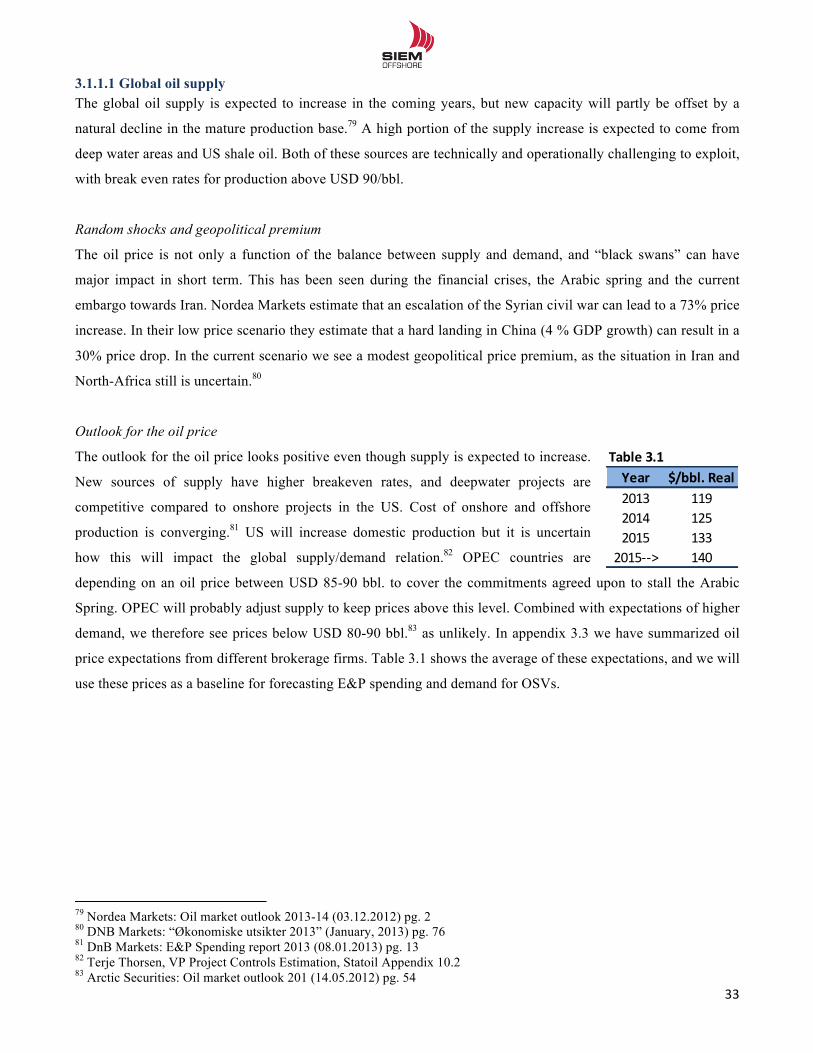
!!
33!!
3.1.1.1 Global oil supply The global oil supply is expected to increase in the coming years, but new capacity will partly be offset by a
natural decline in the mature production base.79 A high portion of the supply increase is expected to come from
deep water areas and US shale oil. Both of these sources are technically and operationally challenging to exploit,
with break even rates for production above USD 90/bbl.
Random shocks and geopolitical premium
The oil price is not only a function of the balance between supply and demand, and “black swans” can have
major impact in short term. This has been seen during the financial crises, the Arabic spring and the current
embargo towards Iran. Nordea Markets estimate that an escalation of the Syrian civil war can lead to a 73% price
increase. In their low price scenario they estimate that a hard landing in China (4 % GDP growth) can result in a
30% price drop. In the current scenario we see a modest geopolitical price premium, as the situation in Iran and
North-Africa still is uncertain.80
Outlook for the oil price
The outlook for the oil price looks positive even though supply is expected to increase.
New sources of supply have higher breakeven rates, and deepwater projects are
competitive compared to onshore projects in the US. Cost of onshore and offshore
production is converging.81 US will increase domestic production but it is uncertain
how this will impact the global supply/demand relation.82 OPEC countries are
depending on an oil price between USD 85-90 bbl. to cover the commitments agreed upon to stall the Arabic
Spring. OPEC will probably adjust supply to keep prices above this level. Combined with expectations of higher
demand, we therefore see prices below USD 80-90 bbl.83 as unlikely. In appendix 3.3 we have summarized oil
price expectations from different brokerage firms. Table 3.1 shows the average of these expectations, and we will
use these prices as a baseline for forecasting E&P spending and demand for OSVs.
!!!!!!!!!!!!!!!!!!!!!!!!!!!!!!!!!!!!!!!!!!!!!!!!!!!!!!!!!!!!!79 Nordea Markets: Oil market outlook 2013-14 (03.12.2012) pg. 2 80 DNB Markets: “Økonomiske utsikter 2013” (January, 2013) pg. 76 81 DnB Markets: E&P Spending report 2013 (08.01.2013) pg. 13 82 Terje Thorsen, VP Project Controls Estimation, Statoil Appendix 10.2 83 Arctic Securities: Oil market outlook 201 (14.05.2012) pg. 54
Table&3.1Year $/bbl.&Real2013 1192014 1252015 133
2015((> 140
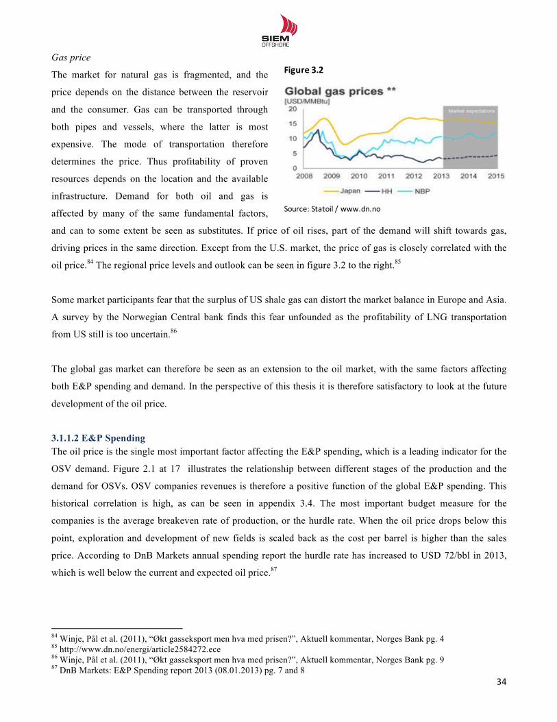
!!
34!!
Gas price
The market for natural gas is fragmented, and the
price depends on the distance between the reservoir
and the consumer. Gas can be transported through
both pipes and vessels, where the latter is most
expensive. The mode of transportation therefore
determines the price. Thus profitability of proven
resources depends on the location and the available
infrastructure. Demand for both oil and gas is
affected by many of the same fundamental factors,
and can to some extent be seen as substitutes. If price of oil rises, part of the demand will shift towards gas,
driving prices in the same direction. Except from the U.S. market, the price of gas is closely correlated with the
oil price.84 The regional price levels and outlook can be seen in figure 3.2 to the right.85
Some market participants fear that the surplus of US shale gas can distort the market balance in Europe and Asia.
A survey by the Norwegian Central bank finds this fear unfounded as the profitability of LNG transportation
from US still is too uncertain.86
The global gas market can therefore be seen as an extension to the oil market, with the same factors affecting
both E&P spending and demand. In the perspective of this thesis it is therefore satisfactory to look at the future
development of the oil price.
3.1.1.2 E&P Spending The oil price is the single most important factor affecting the E&P spending, which is a leading indicator for the
OSV demand. Figure 2.1 at 17 illustrates the relationship between different stages of the production and the
demand for OSVs. OSV companies revenues is therefore a positive function of the global E&P spending. This
historical correlation is high, as can be seen in appendix 3.4. The most important budget measure for the
companies is the average breakeven rate of production, or the hurdle rate. When the oil price drops below this
point, exploration and development of new fields is scaled back as the cost per barrel is higher than the sales
price. According to DnB Markets annual spending report the hurdle rate has increased to USD 72/bbl in 2013,
which is well below the current and expected oil price.87
!!!!!!!!!!!!!!!!!!!!!!!!!!!!!!!!!!!!!!!!!!!!!!!!!!!!!!!!!!!!!84 Winje, Pål et al. (2011), “Økt gasseksport men hva med prisen?”, Aktuell kommentar, Norges Bank pg. 4 85 http://www.dn.no/energi/article2584272.ece 86 Winje, Pål et al. (2011), “Økt gasseksport men hva med prisen?”, Aktuell kommentar, Norges Bank pg. 9 87 DnB Markets: E&P Spending report 2013 (08.01.2013) pg. 7 and 8
Source:(Statoil(/(www.dn.no
Figure 3.2
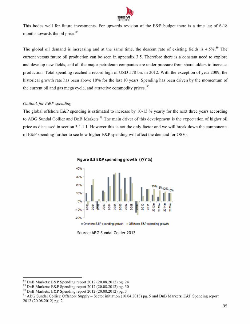
!!
35!!
This bodes well for future investments. For upwards revision of the E&P budget there is a time lag of 6-18
months towards the oil price.88
The global oil demand is increasing and at the same time, the descent rate of existing fields is 4.5%.89 The
current versus future oil production can be seen in appendix 3.5. Therefore there is a constant need to explore
and develop new fields, and all the major petroleum companies are under pressure from shareholders to increase
production. Total spending reached a record high of USD 578 bn. in 2012. With the exception of year 2009, the
historical growth rate has been above 10% for the last 10 years. Spending has been driven by the momentum of
the current oil and gas mega cycle, and attractive commodity prices. 90
Outlook for E&P spending
The global offshore E&P spending is estimated to increase by 10-13 % yearly for the next three years according
to ABG Sundal Collier and DnB Markets.91 The main driver of this development is the expectation of higher oil
price as discussed in section 3.1.1.1. However this is not the only factor and we will break down the components
of E&P spending further to see how higher E&P spending will affect the demand for OSVs.
!
!
!
!!!!!!!!!!!!!!!!!!!!!!!!!!!!!!!!!!!!!!!!!!!!!!!!!!!!!!!!!!!!!88 DnB Markets: E&P Spending report 2012 (20.08.2012) pg. 24 89 DnB Markets: E&P Spending report 2012 (20.08.2012) pg. 30 90 DnB Markets: E&P Spending report 2012 (20.08.2012) pg. 3 91 ABG Sundal Collier: Offshore Supply – Sector initiation (10.04.2013) pg. 5 and DnB Markets: E&P Spending report 2012 (20.08.2012) pg. 2
Figure 3.3)E&P)spending growth (Y/Y)%)
Source:(ABG(Sundal Collier(2013
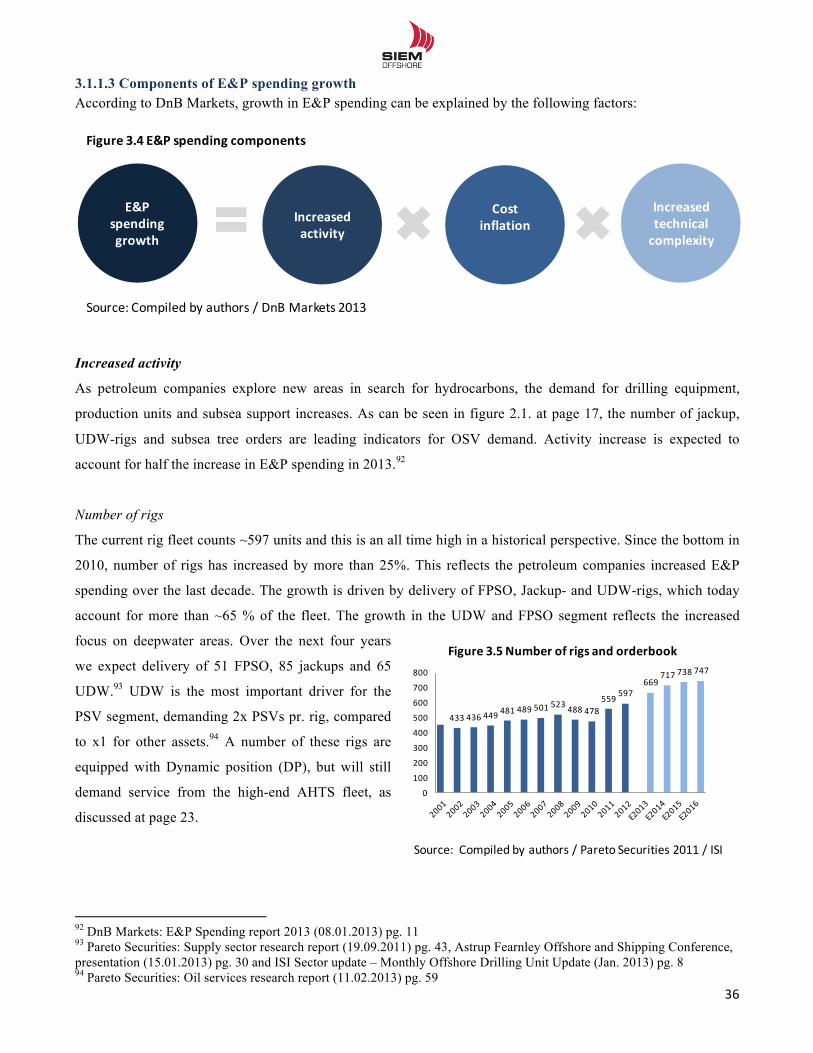
!!
36!!
3.1.1.3 Components of E&P spending growth According to DnB Markets, growth in E&P spending can be explained by the following factors:
Increased activity
As petroleum companies explore new areas in search for hydrocarbons, the demand for drilling equipment,
production units and subsea support increases. As can be seen in figure 2.1. at page 17, the number of jackup,
UDW-rigs and subsea tree orders are leading indicators for OSV demand. Activity increase is expected to
account for half the increase in E&P spending in 2013.92
Number of rigs
The current rig fleet counts ~597 units and this is an all time high in a historical perspective. Since the bottom in
2010, number of rigs has increased by more than 25%. This reflects the petroleum companies increased E&P
spending over the last decade. The growth is driven by delivery of FPSO, Jackup- and UDW-rigs, which today
account for more than ~65 % of the fleet. The growth in the UDW and FPSO segment reflects the increased
focus on deepwater areas. Over the next four years
we expect delivery of 51 FPSO, 85 jackups and 65
UDW.93 UDW is the most important driver for the
PSV segment, demanding 2x PSVs pr. rig, compared
to x1 for other assets.94 A number of these rigs are
equipped with Dynamic position (DP), but will still
demand service from the high-end AHTS fleet, as
discussed at page 23.
!!!!!!!!!!!!!!!!!!!!!!!!!!!!!!!!!!!!!!!!!!!!!!!!!!!!!!!!!!!!!92 DnB Markets: E&P Spending report 2013 (08.01.2013) pg. 11 93 Pareto Securities: Supply sector research report (19.09.2011) pg. 43, Astrup Fearnley Offshore and Shipping Conference, presentation (15.01.2013) pg. 30 and ISI Sector update – Monthly Offshore Drilling Unit Update (Jan. 2013) pg. 8 94 Pareto Securities: Oil services research report (11.02.2013) pg. 59
Increasedactivity
Increasedtechnicalcomplexity
E&P6spendinggrowth
Costinflation
Figure 3.46E&P6spending components
Source:(Compiled by(authors /(DnB Markets(2013
433 436 449481 489 501
523 488 478559 597
669717 738 747
0
100
200
300
400
500
600
700
800
Figure'3.5'Number'of'rigs'and'orderbook
Source:22Compiled by2authors /2Pareto Securities 20112/2ISI
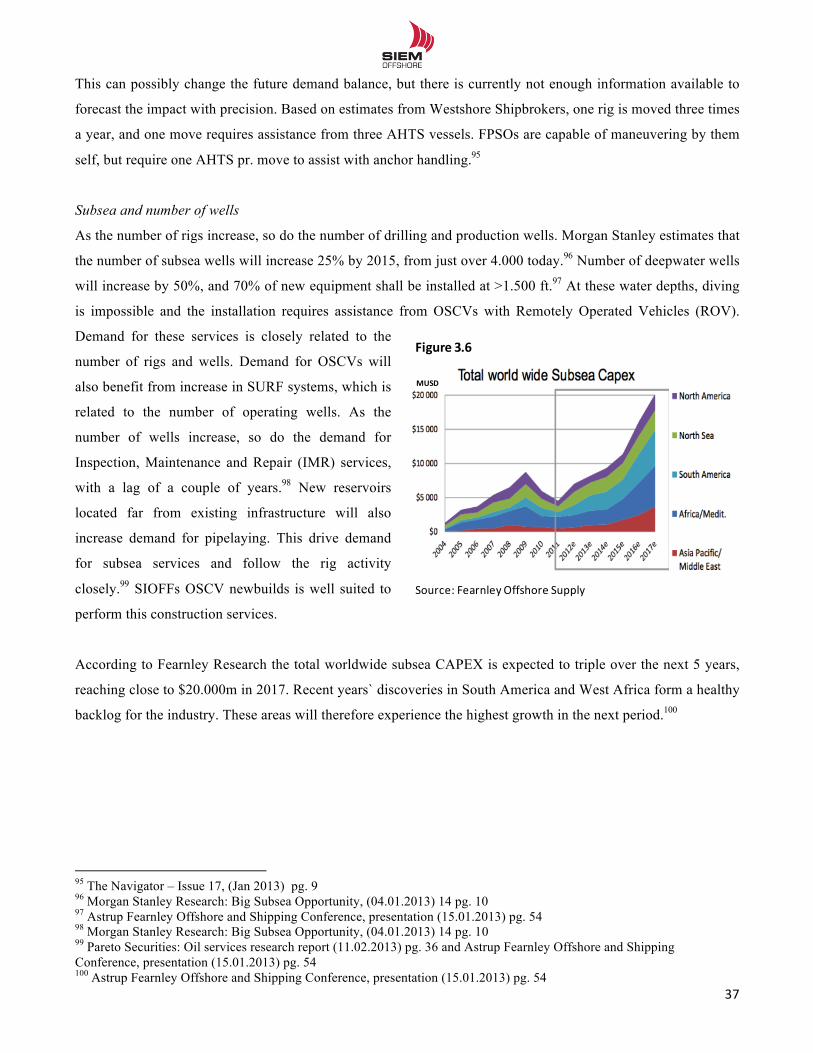
!!
37!!
This can possibly change the future demand balance, but there is currently not enough information available to
forecast the impact with precision. Based on estimates from Westshore Shipbrokers, one rig is moved three times
a year, and one move requires assistance from three AHTS vessels. FPSOs are capable of maneuvering by them
self, but require one AHTS pr. move to assist with anchor handling.95
Subsea and number of wells
As the number of rigs increase, so do the number of drilling and production wells. Morgan Stanley estimates that
the number of subsea wells will increase 25% by 2015, from just over 4.000 today.96 Number of deepwater wells
will increase by 50%, and 70% of new equipment shall be installed at >1.500 ft.97 At these water depths, diving
is impossible and the installation requires assistance from OSCVs with Remotely Operated Vehicles (ROV).
Demand for these services is closely related to the
number of rigs and wells. Demand for OSCVs will
also benefit from increase in SURF systems, which is
related to the number of operating wells. As the
number of wells increase, so do the demand for
Inspection, Maintenance and Repair (IMR) services,
with a lag of a couple of years.98 New reservoirs
located far from existing infrastructure will also
increase demand for pipelaying. This drive demand
for subsea services and follow the rig activity
closely.99 SIOFFs OSCV newbuilds is well suited to
perform this construction services.
According to Fearnley Research the total worldwide subsea CAPEX is expected to triple over the next 5 years,
reaching close to $20.000m in 2017. Recent years` discoveries in South America and West Africa form a healthy
backlog for the industry. These areas will therefore experience the highest growth in the next period.100
!!!!!!!!!!!!!!!!!!!!!!!!!!!!!!!!!!!!!!!!!!!!!!!!!!!!!!!!!!!!!95 The Navigator – Issue 17, (Jan 2013) pg. 9 96 Morgan Stanley Research: Big Subsea Opportunity, (04.01.2013) 14 pg. 10 97 Astrup Fearnley Offshore and Shipping Conference, presentation (15.01.2013) pg. 54 98 Morgan Stanley Research: Big Subsea Opportunity, (04.01.2013) 14 pg. 10 99 Pareto Securities: Oil services research report (11.02.2013) pg. 36 and Astrup Fearnley Offshore and Shipping Conference, presentation (15.01.2013) pg. 54 100 Astrup Fearnley Offshore and Shipping Conference, presentation (15.01.2013) pg. 54
MUSD
Figure 3.6
Source:(Fearnley Offshore(Supply
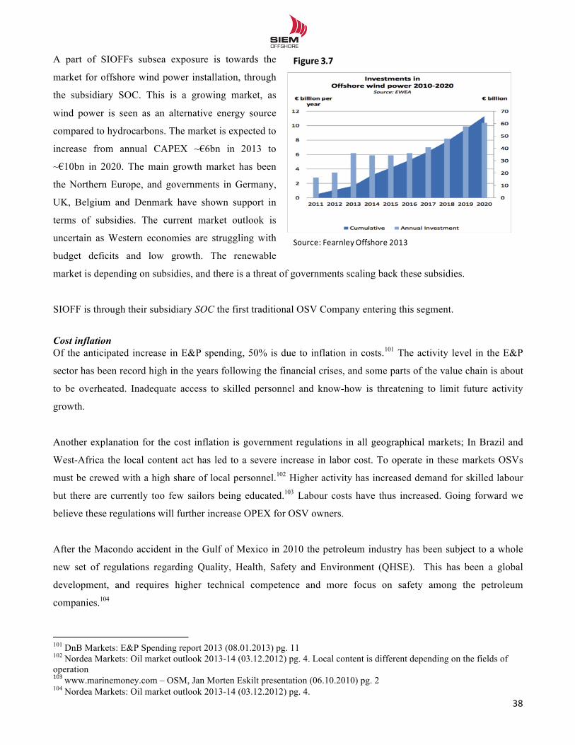
!!
38!!
A part of SIOFFs subsea exposure is towards the
market for offshore wind power installation, through
the subsidiary SOC. This is a growing market, as
wind power is seen as an alternative energy source
compared to hydrocarbons. The market is expected to
increase from annual CAPEX ~€6bn in 2013 to
~€10bn in 2020. The main growth market has been
the Northern Europe, and governments in Germany,
UK, Belgium and Denmark have shown support in
terms of subsidies. The current market outlook is
uncertain as Western economies are struggling with
budget deficits and low growth. The renewable
market is depending on subsidies, and there is a threat of governments scaling back these subsidies.
SIOFF is through their subsidiary SOC the first traditional OSV Company entering this segment.
Cost inflation Of the anticipated increase in E&P spending, 50% is due to inflation in costs.101 The activity level in the E&P
sector has been record high in the years following the financial crises, and some parts of the value chain is about
to be overheated. Inadequate access to skilled personnel and know-how is threatening to limit future activity
growth.
Another explanation for the cost inflation is government regulations in all geographical markets; In Brazil and
West-Africa the local content act has led to a severe increase in labor cost. To operate in these markets OSVs
must be crewed with a high share of local personnel.102 Higher activity has increased demand for skilled labour
but there are currently too few sailors being educated.103 Labour costs have thus increased. Going forward we
believe these regulations will further increase OPEX for OSV owners.
After the Macondo accident in the Gulf of Mexico in 2010 the petroleum industry has been subject to a whole
new set of regulations regarding Quality, Health, Safety and Environment (QHSE). This has been a global
development, and requires higher technical competence and more focus on safety among the petroleum
companies.104
!!!!!!!!!!!!!!!!!!!!!!!!!!!!!!!!!!!!!!!!!!!!!!!!!!!!!!!!!!!!!101 DnB Markets: E&P Spending report 2013 (08.01.2013) pg. 11 102 Nordea Markets: Oil market outlook 2013-14 (03.12.2012) pg. 4. Local content is different depending on the fields of operation 103!www.marinemoney.com – OSM, Jan Morten Eskilt presentation (06.10.2010) pg. 2!104 Nordea Markets: Oil market outlook 2013-14 (03.12.2012) pg. 4.
Figure 3.7
Source:(Fearnley Offshore(2013
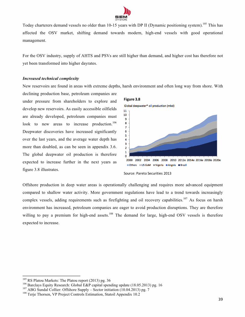
!!
39!!
Today charterers demand vessels no older than 10-15 years with DP II (Dynamic positioning system).105 This has
affected the OSV market, shifting demand towards modern, high-end vessels with good operational
management.
For the OSV industry, supply of AHTS and PSVs are still higher than demand, and higher cost has therefore not
yet been transformed into higher dayrates.
Increased technical complexity
New reservoirs are found in areas with extreme depths, harsh environment and often long way from shore. With
declining production base, petroleum companies are
under pressure from shareholders to explore and
develop new reservoirs. As easily accessible oilfields
are already developed, petroleum companies must
look to new areas to increase production.106
Deepwater discoveries have increased significantly
over the last years, and the average water depth has
more than doubled, as can be seen in appendix 3.6.
The global deepwater oil production is therefore
expected to increase further in the next years as
figure 3.8 illustrates.
Offshore production in deep water areas is operationally challenging and requires more advanced equipment
compared to shallow water activity. More government regulations have lead to a trend towards increasingly
complex vessels, adding requirements such as firefighting and oil recovery capabilities.107 As focus on harsh
environment has increased, petroleum companies are eager to avoid production disruptions. They are therefore
willing to pay a premium for high-end assets.108 The demand for large, high-end OSV vessels is therefore
expected to increase.
!!!!!!!!!!!!!!!!!!!!!!!!!!!!!!!!!!!!!!!!!!!!!!!!!!!!!!!!!!!!!105 RS Platou Markets: The Platou report (2013) pg. 36 106 Barclays Equity Research: Global E&P capital spending update (18.05.2013) pg. 16 107 ABG Sundal Collier: Offshore Supply – Sector initiation (10.04.2013) pg. 7 108 Terje Thorsen, VP Project Controls Estimation, Statoil Appendix 10.2
Figure 3.8
Source:(Pareto Securities 2013
!!
40!!
3.1.1.3 Regional demand
North Sea
The North Sea is one of the most developed offshore regions, with declining production rate. Today the region
has started to regain some momentum as a result of recent exploration successes and new fields coming on-
stream during the next few years.109 Petroleum companies have therefore increased their exploration activities,
and E&P spending is expected to increase by 6% in 2013.110 More than 50 % of the high-end PSV fleet operates
in the North Sea, reflecting the high production activity. As exploration has increased, ~20% of the high-end
AHTS fleet is also present.
The water depths are challenging, but the main difference from other regions is the extreme weather conditions
and harsh environment. For years petroleum companies has therefore requested large and sophisticated vessels.
High-end vessels have therefore been termed “North Sea assets”, but today this demand-trend is also important
in Gulf of Mexico, Brazil and West Africa.111 This is a result of government regulations, and as Norwegian OSV
companies are used to own and operate this kind of vessels they might have an advantage.
America
Offshore E&P activity at the American continent has been rather unstable over the last five years. After the
Macondo accident in 2010 all exploration activity was postponed. At the same time major reservoirs was
discovered at the Brazilian continental shelf. This led to a boom in Brazilian activity. New regulations are now in
place in the Gulf of Mexico and petroleum companies are optimistic for future activity. Despite this, E&P
spending is not expected to increase in 2013. This is not the case for Brazil, where several projects are expected
to come on-stream over the next years. E&P spending is therefore expected to increase by 15% in 2013. Demand
from Petrobras has been the main driver for the Brazilian OSV industry, but the company has now announced
reduced future growth as a result of an overheated industry. The long term prospects for the region has therefore
been somewhat lowered, reducing the attractiveness of the region.112
The American continent is the most important market for UDW rigs, currently employing 83 units. This is due to
the extreme water depths. Outside Brazil the distance between surface and reservoir can be more than 7000m.
The region is therefore the largest market for high-end AHTS, with 34% of the fleet in operation. Because of the
long offshore distance and high activity, ~40 % of the high-end PSV fleet is also present.
!!!!!!!!!!!!!!!!!!!!!!!!!!!!!!!!!!!!!!!!!!!!!!!!!!!!!!!!!!!!!109 DnB Markets: E&P Spending report 2012 (20.08.2012) pg. 35 110 TTGS Nopec Geophysical Company – Guidance announcement (08.01.2013) pg. 5 111 Pareto Securities: Oil services research report (11.02.2013) pg.. 58 112 ABG Sundal Collier: Offshore Supply – Sector initiation (10.04.2013) pg. 12, Pareto Securities: Oil services research report (11.02.2013) pg. 54
!!
41!!
West Africa
The West African region has been the second most important growth regions for the offshore industry over the
last decade. As growth in Brazil is expected to slow down, West Africa is among the most promising regions
going forward. With ocean depth from 1000 – 2100m the region has been an important driver for the deepwater
development, especially for the subsea segment. There are currently~30 UDW rigs in the region, employing 20%
of the high-end AHTS fleet. The region is still in the development face which explains why only ~7% of the
high-end PSV fleet operates here.113 Barclay’s Capital expects the E&P spending for the region to increase by
4.5% in 2013.114
Although the outlook for the West African region has been buoyant for years, there have been numerous project
delays affecting the growth rate. Local governments have struggled with a dysfunctional approval process for
new oil laws and conflicting interest with IOCs and NOCs.115 Political bureaucracy and uncertainty for local
content is the biggest concern going forward.116 Despite this, West Africa is the most important growth region,
and the main question is the timing rather than the potential.117
3.1.1.5 Summary – Demand for OSV The oil price is the most important factor affecting the global E&P spending, which is a leading indicator for
OSV demand. Based on fundamental factors such as higher GDP growth and modest supply increase, the oil
price is expected to incline from today´s level. New production has break even rates above $80/bbl., which we
see as a lower bound for the price. The average current hurdle rate of production is $72/bbl providing a strong
cash flow for the petroleum companies. This bodes well for growth in E&P spending which is expected to
increase by 13% in 2013. Petroleum companies are under pressure to increase production, and activity is shifted
towards deepwater areas with harsh environment. Together with increased technical, safety and environmental
focus we therefore see strong demand for modern, high-end vessels. The high-end AHTS segment will be driven
by a 25% growth in rig deliveries and the high-end PSV segment will in addition be driven by increased
production activity. The demand for subsea services is also expected to increase significantly, as CAPX will
more than triple over the next 5 years.
The development is fueled by the high number of deepwater installations and renewable energy projects. Overall
we expect demand for OSVs to increase by ~20 – 30 % over the next four years.
!!!!!!!!!!!!!!!!!!!!!!!!!!!!!!!!!!!!!!!!!!!!!!!!!!!!!!!!!!!!!113 Pareto Securities: Oil services research report (11.02.2013) pg. 63 and 64 114 TTGS Nopec Geophysical Company – Guidance announcement (08.01.2013) pg. 5 115 Pareto Securities: Oil services research report (11.02.2013) pg. 39 116 Pareto Securities: Oil services research report (11.02.2013) pg. 39 117 Pareto Securities: Oil services research report (11.02.2013) pg. 38
!!
42!!
3.1.2 Supply of OSV The supply of OSVs is characterized as slow in response to changes in demand. This is due to the construction
time of vessels which range from 1-3 years, depending on vessel type and yard capacity.118 In this section, we
aim to explain and analyze the factors affecting supply.
3.1.2.1 Five decision makers The supply of vessels is controlled or influenced by four groups of decision makers: shipowners,
shippers/charterers, bankers/financial institutions and regulatory authorities.119 In addition, shipyards are seen as
a fifth decision-maker.120 Because of the nature of these decision-makers, the supply-side relationship in the
model is behavioral and difficult to predict. Table 3.2 summarizes the influence these parties have on supply and
how we see the situation today.
Influence from shipyards and government regulations, will be further analyzed in Porter´s Five Forces.
!!!!!!!!!!!!!!!!!!!!!!!!!!!!!!!!!!!!!!!!!!!!!!!!!!!!!!!!!!!!!118 Stopford, Martin (2009). Maritime Economics 3rd ed. pg. 150, Interview Simen Granerød appendix 10.3 119 Stopford, Martin (2009). Maritime Economics 3rd ed. pg. 150 120Interview Simen Granerød, Clarksons Shipbrokers, appendix 10.3
Decision(maker Influence1on1Supply Current1situationShipowners Order new vessels when the market is expected
to improve, and decide when to scrap old ones. Always seek for profit.
Weak market yields low cash flow and return on capital below WACC. Shareholders unlikely to contribute funds other than at great discounts. High leverage.
Shippers/charterers May stimulate new orders by issuing long-term time charters or become shipowners themselves
Shippers mainly use the spot market, decreasing new orders.
Financial1institutions Access to debt affects to which extent shipowners can invest in new vessels. In a weak market both access and service of debt is limited, reducing supply growth and might lead to scrapping
Lending institutions unwilling to provide debt.Norwegian export financing agency reduce debt available to fund construction of PSVsHowever, well functioning high-yield market in Norway.
Regulatory1Authorities Affect supply through new safety and environmental legislations.Regional regulations
Local content regulations.Requirements for fire fighting, HSEQ and environmental impact
Shipyards CapacityCabability / know-how
Asian yards build on speculation, increasing the supply (PSVs and less sophisticated vessels).Limited numbers of shipyards that are capable of building high-end vessels
Table 3.2
Source:1Compiled by1authors
!!
43!!
3.1.2.2 The total World Fleet
The current fleet of AHTS and PSVs counts 1897 and 1190 vessels.121 There has been a substantial amount of
newbuilds in recent years, where the PSV fleet has grown by an average of 60 vessels pr year since 2000. This
growth can be explained by the booming dayrates between 2001-2003 and 2006-2008, caused by the high growth
in E&P spending. In a booming market, vessel owner’s cash flow increase significantly and stimulate their
interest in fleet expansion. This behavioral pattern is characteristic for all shipping segments.122 Because of the
financial crisis, many newbuilds were delayed and first delivered during 2009 and 2010. This had major impact
on the dayrates as figure 3.18 on page 49 illustrates.
In the subsea segment there has been a large influx of
capacity since 2008 and up till today. The largest
increase is seen in the ROV support and pipelay
segment. This reflects the findings in the demand
section, as demand for subsea installations is
increasing in deepwater areas.123
!!!!!!!!!!!!!!!!!!!!!!!!!!!!!!!!!!!!!!!!!!!!!!!!!!!!!!!!!!!!!121 Pareto Securities: Oil services research report (11.02.2013) pg. 64 122 Stopford, Martin (2009). Maritime Economics 3rd ed. pg 134. 123 Pareto Securities: Oil services research report (11.02.2013) pg. 47
Figure 3.9
Source:(Pareto Securities2013
Figure 3.10
Source:(Pareto Securities 2013
!!
44!!
3.1.2.3 Newbuilding The OSV market is undergoing a structural shift towards modern, high-end vessels. In this section we will
analyze the current orderbook for the different segments, and determine the expected supply growth. The
underlying date behind the graphs can be seen appendix 3.7.
PSV and newbuilds
The current PSV orderbook is historically high and
the fleet is expected to grow by as much as 27% over
the next two years.124 If we look at the high-end
segment, the orderbook is higher than the existing
fleet, counting a total number of 214 vessels.
However, it is not expected that all vessels will be
delivered, as cancellation and postponements is
common. The high orderbook is a direct result of the
shift in demand towards modern, high-end vessels.
Even though the activity is expected to increase, the influx of newbuildings might put further pressure on the
market. Asian built vessels will increase competition in areas such as Brazil and West Africa, and there is a fear
that Asia shipyards will construct additional vessels on speculation of better market.125 These factors will be
further analyzed through Porters 5 Forces.
AHTS and newbuilds
For the AHTS segment there has been lower ordering
of newbuilds in 2013, and consequently the
orderbook stands at 9% of existing fleet.126 The
highest relative growth is expected in the high-end
segment, where the orderbook is 24% or 44 vessels.
As we will see in the industry analysis, there are a
limited number of shipyards capable of building
high-end vessels.127 The risk of the segment being
overbuilt is therefore low, but as the market tightens,
more vessels will be ordered by eager vessel owners.
Subsea and newbuilds
!!!!!!!!!!!!!!!!!!!!!!!!!!!!!!!!!!!!!!!!!!!!!!!!!!!!!!!!!!!!!124 Astrup Fearnley Offshore and Shipping Conference, presentation (15.01.2013) pg 58, high-end > 5,000 dwt 125 Pareto Securities: Oil services research report (11.02.2013) pg. 59 and Porters 5 Forces 126 Astrup Fearnley Offshore and Shipping Conference, presentation (15.01.2013) pg. 57, high-end > 16,000 BHP 127 Discussed under Porter´s Five Forces.
0
5
10
15
20
25
30
35
0
50
100
150
200
250
300
350
400
450
1000' 1499 1,500' 1,999 2,000' 3,499*dwt
3,500'4,999 5,000*+
Num
ber'o
f'vessels
Average'
age
Figure'3.11'PSV'world'wide'fleet'and'orderbook
Existing*vessels Under*construction Average*age
Source:*Fearnley Offshore*2013
0
5
10
15
20
25
0
200
400
600
800
1000
1200
1400
1600
3,000*7,999 8,000* 11,999 12,000* 15,999 16,000-+
Num
ber'o
f'vessels
Average'
age
Figure'3.12'AHTS'world'wide'fleet'and'orderbook
Existing-vessels Under-construction Average-age
bhp
Source:-Fearnley Offshore-2013
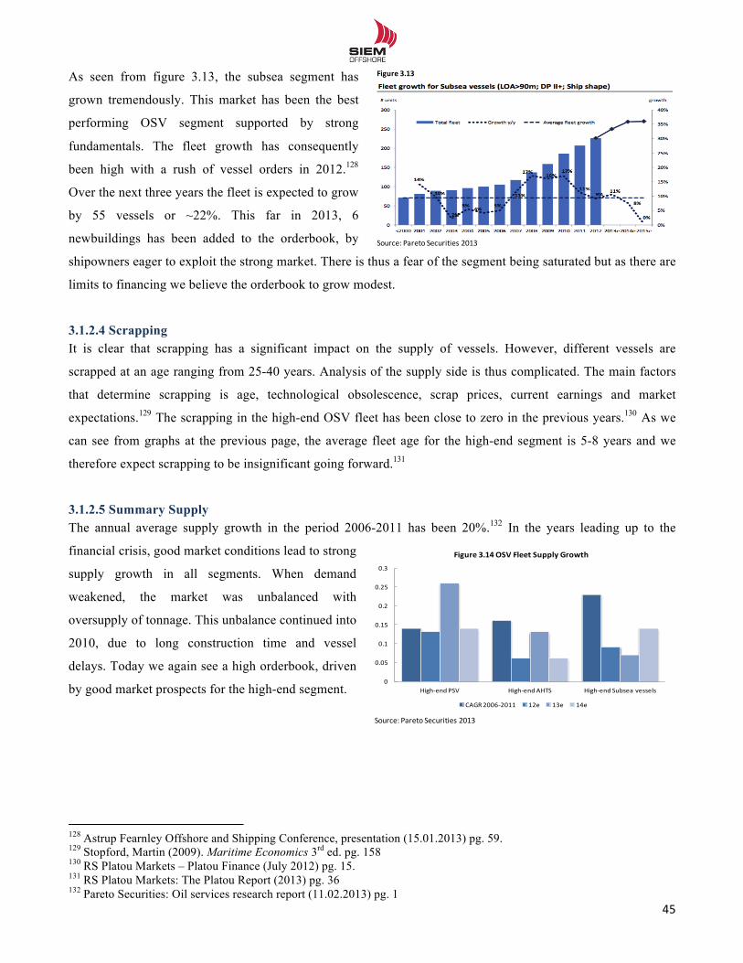
!!
45!!
As seen from figure 3.13, the subsea segment has
grown tremendously. This market has been the best
performing OSV segment supported by strong
fundamentals. The fleet growth has consequently
been high with a rush of vessel orders in 2012.128
Over the next three years the fleet is expected to grow
by 55 vessels or ~22%. This far in 2013, 6
newbuildings has been added to the orderbook, by
shipowners eager to exploit the strong market. There is thus a fear of the segment being saturated but as there are
limits to financing we believe the orderbook to grow modest.
3.1.2.4 Scrapping It is clear that scrapping has a significant impact on the supply of vessels. However, different vessels are
scrapped at an age ranging from 25-40 years. Analysis of the supply side is thus complicated. The main factors
that determine scrapping is age, technological obsolescence, scrap prices, current earnings and market
expectations.129 The scrapping in the high-end OSV fleet has been close to zero in the previous years.130 As we
can see from graphs at the previous page, the average fleet age for the high-end segment is 5-8 years and we
therefore expect scrapping to be insignificant going forward.131
3.1.2.5 Summary Supply The annual average supply growth in the period 2006-2011 has been 20%.132 In the years leading up to the
financial crisis, good market conditions lead to strong
supply growth in all segments. When demand
weakened, the market was unbalanced with
oversupply of tonnage. This unbalance continued into
2010, due to long construction time and vessel
delays. Today we again see a high orderbook, driven
by good market prospects for the high-end segment.
!!!!!!!!!!!!!!!!!!!!!!!!!!!!!!!!!!!!!!!!!!!!!!!!!!!!!!!!!!!!!128 Astrup Fearnley Offshore and Shipping Conference, presentation (15.01.2013) pg. 59. 129 Stopford, Martin (2009). Maritime Economics 3rd ed. pg. 158 130 RS Platou Markets – Platou Finance (July 2012) pg. 15. 131 RS Platou Markets: The Platou Report (2013) pg. 36 132 Pareto Securities: Oil services research report (11.02.2013) pg. 1
Figure 3.13
Source:(Pareto Securities 2013
Source:(Pareto Securities 2013
0
0.05
0.1
0.15
0.2
0.25
0.3
High7end(PSV High7end(AHTS High7end(Subsea(vessels
Figure'3.14'OSV'Fleet'Supply'Growth
CAGR(200672011 12e 13e 14e
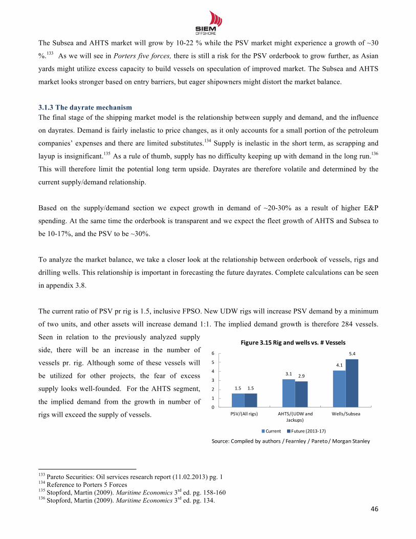
!!
46!!
The Subsea and AHTS market will grow by 10-22 % while the PSV market might experience a growth of ~30
%.133 As we will see in Porters five forces, there is still a risk for the PSV orderbook to grow further, as Asian
yards might utilize excess capacity to build vessels on speculation of improved market. The Subsea and AHTS
market looks stronger based on entry barriers, but eager shipowners might distort the market balance.
3.1.3 The dayrate mechanism The final stage of the shipping market model is the relationship between supply and demand, and the influence
on dayrates. Demand is fairly inelastic to price changes, as it only accounts for a small portion of the petroleum
companies’ expenses and there are limited substitutes.134 Supply is inelastic in the short term, as scrapping and
layup is insignificant.135 As a rule of thumb, supply has no difficulty keeping up with demand in the long run.136
This will therefore limit the potential long term upside. Dayrates are therefore volatile and determined by the
current supply/demand relationship.
Based on the supply/demand section we expect growth in demand of ~20-30% as a result of higher E&P
spending. At the same time the orderbook is transparent and we expect the fleet growth of AHTS and Subsea to
be 10-17%, and the PSV to be ~30%.
To analyze the market balance, we take a closer look at the relationship between orderbook of vessels, rigs and
drilling wells. This relationship is important in forecasting the future dayrates. Complete calculations can be seen
in appendix 3.8.
The current ratio of PSV pr rig is 1.5, inclusive FPSO. New UDW rigs will increase PSV demand by a minimum
of two units, and other assets will increase demand 1:1. The implied demand growth is therefore 284 vessels.
Seen in relation to the previously analyzed supply
side, there will be an increase in the number of
vessels pr. rig. Although some of these vessels will
be utilized for other projects, the fear of excess
supply looks well-founded. For the AHTS segment,
the implied demand from the growth in number of
rigs will exceed the supply of vessels.
!!!!!!!!!!!!!!!!!!!!!!!!!!!!!!!!!!!!!!!!!!!!!!!!!!!!!!!!!!!!!133 Pareto Securities: Oil services research report (11.02.2013) pg. 1 134 Reference to Porters 5 Forces 135 Stopford, Martin (2009). Maritime Economics 3rd ed. pg. 158-160 136 Stopford, Martin (2009). Maritime Economics 3rd ed. pg. 134.
1.5
3.1
4.1
1.5
2.9
5.4
0
1
2
3
4
5
6
PSV/(All1rigs) AHTS/(UDW1and1Jackups)
Wells/Subsea
Figure'3.15'Rig'and'wells'vs.'#'Vessels
Current Future1(2013I17)
Source:1Compiled by1authors /1Fearnley /1Pareto/1Morgan1Stanley
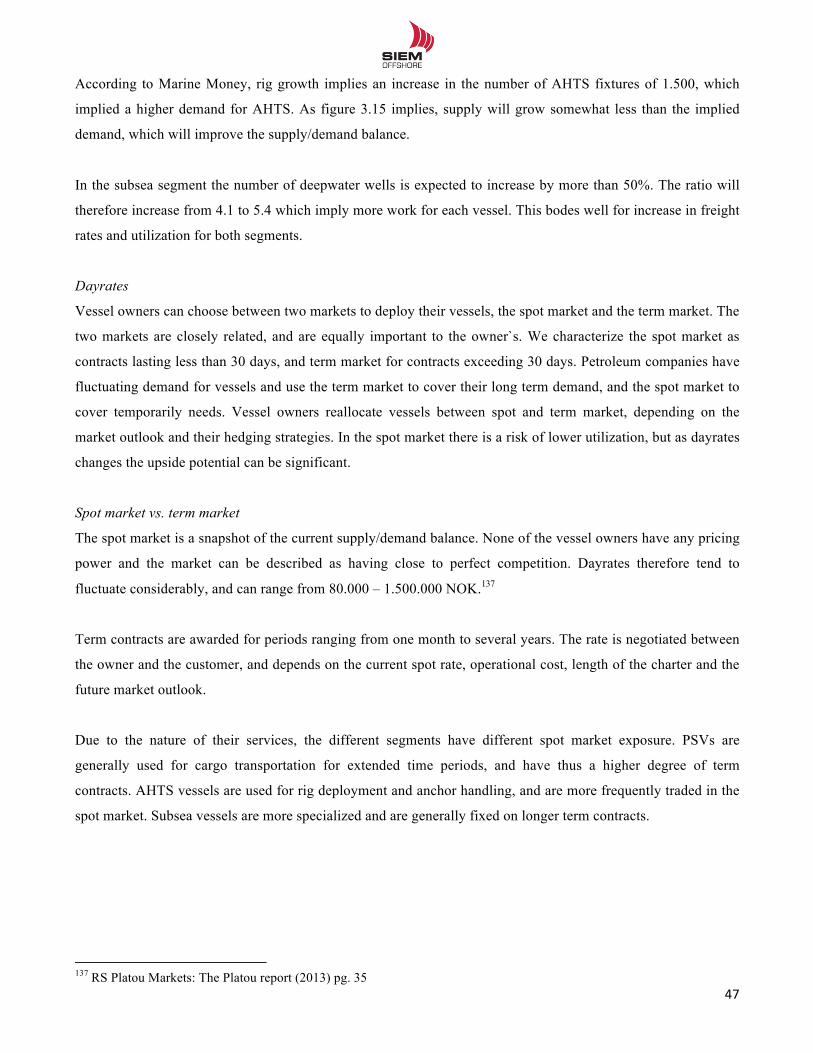
!!
47!!
According to Marine Money, rig growth implies an increase in the number of AHTS fixtures of 1.500, which
implied a higher demand for AHTS. As figure 3.15 implies, supply will grow somewhat less than the implied
demand, which will improve the supply/demand balance.
In the subsea segment the number of deepwater wells is expected to increase by more than 50%. The ratio will
therefore increase from 4.1 to 5.4 which imply more work for each vessel. This bodes well for increase in freight
rates and utilization for both segments.
Dayrates
Vessel owners can choose between two markets to deploy their vessels, the spot market and the term market. The
two markets are closely related, and are equally important to the owner`s. We characterize the spot market as
contracts lasting less than 30 days, and term market for contracts exceeding 30 days. Petroleum companies have
fluctuating demand for vessels and use the term market to cover their long term demand, and the spot market to
cover temporarily needs. Vessel owners reallocate vessels between spot and term market, depending on the
market outlook and their hedging strategies. In the spot market there is a risk of lower utilization, but as dayrates
changes the upside potential can be significant.
Spot market vs. term market
The spot market is a snapshot of the current supply/demand balance. None of the vessel owners have any pricing
power and the market can be described as having close to perfect competition. Dayrates therefore tend to
fluctuate considerably, and can range from 80.000 – 1.500.000 NOK.137
Term contracts are awarded for periods ranging from one month to several years. The rate is negotiated between
the owner and the customer, and depends on the current spot rate, operational cost, length of the charter and the
future market outlook.
Due to the nature of their services, the different segments have different spot market exposure. PSVs are
generally used for cargo transportation for extended time periods, and have thus a higher degree of term
contracts. AHTS vessels are used for rig deployment and anchor handling, and are more frequently traded in the
spot market. Subsea vessels are more specialized and are generally fixed on longer term contracts.
!!!!!!!!!!!!!!!!!!!!!!!!!!!!!!!!!!!!!!!!!!!!!!!!!!!!!!!!!!!!!137 RS Platou Markets: The Platou report (2013) pg. 35
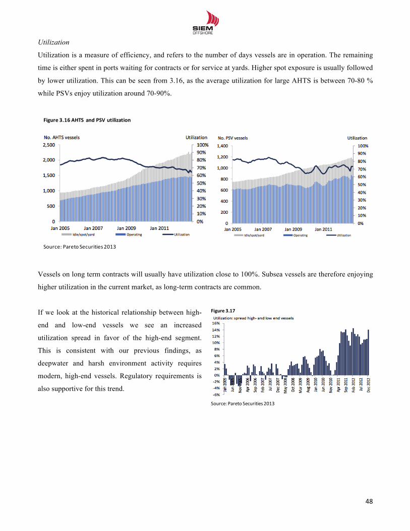
!!
48!!
Utilization
Utilization is a measure of efficiency, and refers to the number of days vessels are in operation. The remaining
time is either spent in ports waiting for contracts or for service at yards. Higher spot exposure is usually followed
by lower utilization. This can be seen from 3.16, as the average utilization for large AHTS is between 70-80 %
while PSVs enjoy utilization around 70-90%.
Vessels on long term contracts will usually have utilization close to 100%. Subsea vessels are therefore enjoying
higher utilization in the current market, as long-term contracts are common.
If we look at the historical relationship between high-
end and low-end vessels we see an increased
utilization spread in favor of the high-end segment.
This is consistent with our previous findings, as
deepwater and harsh environment activity requires
modern, high-end vessels. Regulatory requirements is
also supportive for this trend.
Source:(Pareto(Securities2013
Figure 3.16+AHTS+ and+PSV+utilization
Figure 3.17
Source:(Pareto Securities 2013
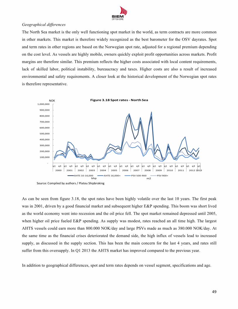
!!
49!!
Geographical differences
The North Sea market is the only well functioning spot market in the world, as term contracts are more common
in other markets. This market is therefore widely recognized as the best barometer for the OSV dayrates. Spot
and term rates in other regions are based on the Norwegian spot rate, adjusted for a regional premium depending
on the cost level. As vessels are highly mobile, owners quickly exploit profit opportunities across markets. Profit
margins are therefore similar. This premium reflects the higher costs associated with local content requirements,
lack of skilled labor, political instability, bureaucracy and taxes. Higher costs are also a result of increased
environmental and safety requirements. A closer look at the historical development of the Norwegian spot rates
is therefore representative.
As can be seen from figure 3.18, the spot rates have been highly volatile over the last 10 years. The first peak
was in 2001, driven by a good financial market and subsequent higher E&P spending. This boom was short lived
as the world economy went into recession and the oil price fell. The spot market remained depressed until 2005,
when higher oil price fueled E&P spending. As supply was modest, rates reached an all time high. The largest
AHTS vessels could earn more than 800.000 NOK/day and large PSVs made as much as 380.000 NOK/day. At
the same time as the financial crises deteriorated the demand side, the high influx of vessels lead to increased
supply, as discussed in the supply section. This has been the main concern for the last 4 years, and rates still
suffer from this oversupply. In Q1 2013 the AHTS market has improved compared to the previous year.
In addition to geographical differences, spot and term rates depends on vessel segment, specifications and age.
!
NOK
Source:+Compiled by+authors /+Platou+Shipbroking
=
100,000+
200,000+
300,000+
400,000+
500,000+
600,000+
700,000+
800,000+
900,000+
1,000,000+
q1 q3 q1 q3 q1 q3 q1 q3 q1 q3 q1 q3 q1 q3 q1 q3 q1 q3 q1 q3 q1 q3 q1 q3 q1 q3 q1
2000 2001 2002 2003 2004 2005 2006 2007 2008 2009 2010 2011 2012 2013
Figure'3.18'Spot'rates'2 North'Sea
AHTS+10=16,000 AHTS+16,000+ PSV+500=900 PSV+900+bhp m2
!!
50!!
3.1.4 Conclusion to the shipping market model The oil price is expected to increase going forward, based on higher GDP growth and limited growth in supply.
Petroleum companies will increase their E&P budget based on this development, as they need to both replace
and grow their current production. As the easy available resources have been exploited, activity will move
towards deepwater and harsh environment areas. Number of deepwater wells is therefore expected to increase by
50%, and based on the current orderbook we see more than 170 rig/production units entering the market. This
will increase demand for OSV services by 20-30% over the next four years, in particular the high-end segment.
The newbuilding orderbook is transparent and we see a supply growth of 10-22% for the high-end AHTS and
OSCV segment. We therefore expect dayrates and utilization to increase from today`s level. Higher activity will
also bode well for increased high-end PSV demand, and the utilization spread is in favor of high-end vessels. But
as the orderbook implies a supply growth of ~30%, we are afraid of a weak market balance affecting dayrates
and utilization for PSVs going forward.
!
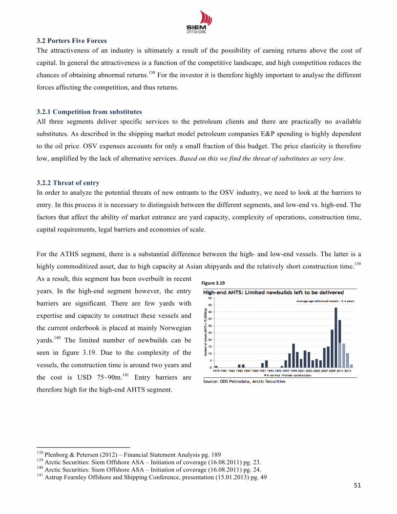
!!
51!!
3.2 Porters Five Forces The attractiveness of an industry is ultimately a result of the possibility of earning returns above the cost of
capital. In general the attractiveness is a function of the competitive landscape, and high competition reduces the
chances of obtaining abnormal returns.138 For the investor it is therefore highly important to analyse the different
forces affecting the competition, and thus returns.
3.2.1 Competition from substitutes All three segments deliver specific services to the petroleum clients and there are practically no available
substitutes. As described in the shipping market model petroleum companies E&P spending is highly dependent
to the oil price. OSV expenses accounts for only a small fraction of this budget. The price elasticity is therefore
low, amplified by the lack of alternative services. Based on this we find the threat of substitutes as very low.
3.2.2 Threat of entry In order to analyze the potential threats of new entrants to the OSV industry, we need to look at the barriers to
entry. In this process it is necessary to distinguish between the different segments, and low-end vs. high-end. The
factors that affect the ability of market entrance are yard capacity, complexity of operations, construction time,
capital requirements, legal barriers and economies of scale.
For the ATHS segment, there is a substantial difference between the high- and low-end vessels. The latter is a
highly commoditized asset, due to high capacity at Asian shipyards and the relatively short construction time.139
As a result, this segment has been overbuilt in recent
years. In the high-end segment however, the entry
barriers are significant. There are few yards with
expertise and capacity to construct these vessels and
the current orderbook is placed at mainly Norwegian
yards.140 The limited number of newbuilds can be
seen in figure 3.19. Due to the complexity of the
vessels, the construction time is around two years and
the cost is USD 75~90m.141 Entry barriers are
therefore high for the high-end AHTS segment.
!!!!!!!!!!!!!!!!!!!!!!!!!!!!!!!!!!!!!!!!!!!!!!!!!!!!!!!!!!!!!138 Plenborg & Petersen (2012) – Financial Statement Analysis pg. 189 139 Arctic Securities: Siem Offshore ASA – Initiation of coverage (16.08.2011) pg. 23. 140 Arctic Securities: Siem Offshore ASA – Initiation of coverage (16.08.2011) pg. 24. 141 Astrup Fearnley Offshore and Shipping Conference, presentation (15.01.2013) pg. 49
Figure 3.19
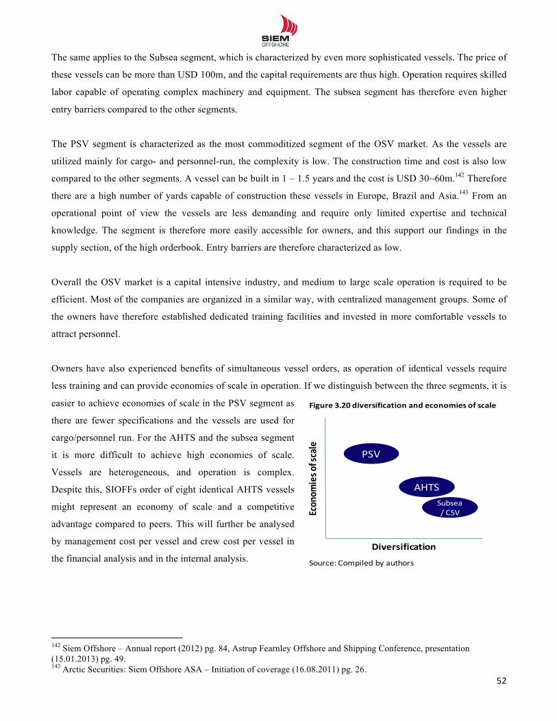
!!
52!!
The same applies to the Subsea segment, which is characterized by even more sophisticated vessels. The price of
these vessels can be more than USD 100m, and the capital requirements are thus high. Operation requires skilled
labor capable of operating complex machinery and equipment. The subsea segment has therefore even higher
entry barriers compared to the other segments.
The PSV segment is characterized as the most commoditized segment of the OSV market. As the vessels are
utilized mainly for cargo- and personnel-run, the complexity is low. The construction time and cost is also low
compared to the other segments. A vessel can be built in 1 – 1.5 years and the cost is USD 30~60m.142 Therefore
there are a high number of yards capable of construction these vessels in Europe, Brazil and Asia.143 From an
operational point of view the vessels are less demanding and require only limited expertise and technical
knowledge. The segment is therefore more easily accessible for owners, and this support our findings in the
supply section, of the high orderbook. Entry barriers are therefore characterized as low.
Overall the OSV market is a capital intensive industry, and medium to large scale operation is required to be
efficient. Most of the companies are organized in a similar way, with centralized management groups. Some of
the owners have therefore established dedicated training facilities and invested in more comfortable vessels to
attract personnel.
Owners have also experienced benefits of simultaneous vessel orders, as operation of identical vessels require
less training and can provide economies of scale in operation. If we distinguish between the three segments, it is
easier to achieve economies of scale in the PSV segment as
there are fewer specifications and the vessels are used for
cargo/personnel run. For the AHTS and the subsea segment
it is more difficult to achieve high economies of scale.
Vessels are heterogeneous, and operation is complex.
Despite this, SIOFFs order of eight identical AHTS vessels
might represent an economy of scale and a competitive
advantage compared to peers. This will further be analysed
by management cost per vessel and crew cost per vessel in
the financial analysis and in the internal analysis.
!!!!!!!!!!!!!!!!!!!!!!!!!!!!!!!!!!!!!!!!!!!!!!!!!!!!!!!!!!!!!142 Siem Offshore – Annual report (2012) pg. 84, Astrup Fearnley Offshore and Shipping Conference, presentation (15.01.2013) pg. 49. 143 Arctic Securities: Siem Offshore ASA – Initiation of coverage (16.08.2011) pg. 26.
AHTS
PSV
Subsea/-CSV
Diversification
Econ
omieso
f/scale
Figure 3.20/diversification and/economies of/scale
Source:-Compiled by-authors
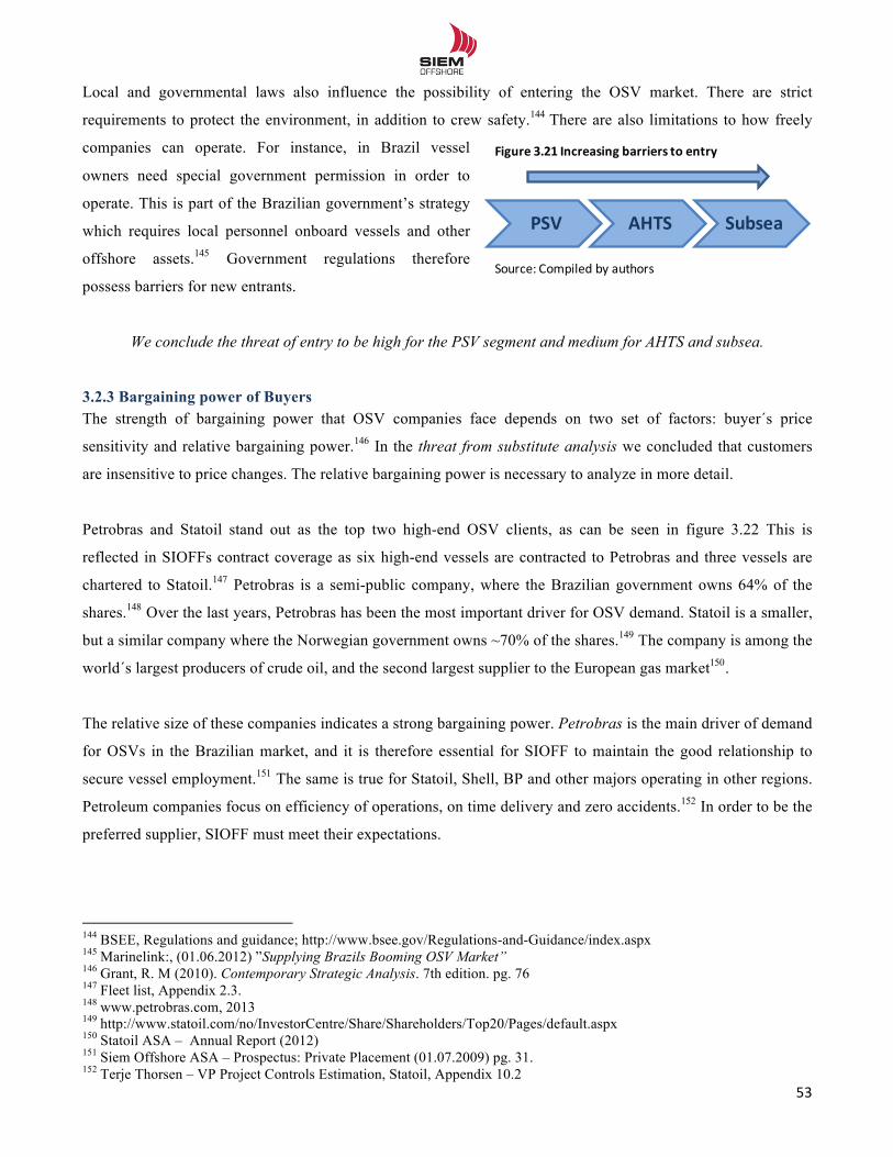
!!
53!!
Local and governmental laws also influence the possibility of entering the OSV market. There are strict
requirements to protect the environment, in addition to crew safety.144 There are also limitations to how freely
companies can operate. For instance, in Brazil vessel
owners need special government permission in order to
operate. This is part of the Brazilian government’s strategy
which requires local personnel onboard vessels and other
offshore assets.145 Government regulations therefore
possess barriers for new entrants.
We conclude the threat of entry to be high for the PSV segment and medium for AHTS and subsea.
3.2.3 Bargaining power of Buyers The strength of bargaining power that OSV companies face depends on two set of factors: buyer´s price
sensitivity and relative bargaining power.146 In the threat from substitute analysis we concluded that customers
are insensitive to price changes. The relative bargaining power is necessary to analyze in more detail.
Petrobras and Statoil stand out as the top two high-end OSV clients, as can be seen in figure 3.22 This is
reflected in SIOFFs contract coverage as six high-end vessels are contracted to Petrobras and three vessels are
chartered to Statoil.147 Petrobras is a semi-public company, where the Brazilian government owns 64% of the
shares.148 Over the last years, Petrobras has been the most important driver for OSV demand. Statoil is a smaller,
but a similar company where the Norwegian government owns ~70% of the shares.149 The company is among the
world´s largest producers of crude oil, and the second largest supplier to the European gas market150.
The relative size of these companies indicates a strong bargaining power. Petrobras is the main driver of demand
for OSVs in the Brazilian market, and it is therefore essential for SIOFF to maintain the good relationship to
secure vessel employment.151 The same is true for Statoil, Shell, BP and other majors operating in other regions.
Petroleum companies focus on efficiency of operations, on time delivery and zero accidents.152 In order to be the
preferred supplier, SIOFF must meet their expectations.
!!!!!!!!!!!!!!!!!!!!!!!!!!!!!!!!!!!!!!!!!!!!!!!!!!!!!!!!!!!!!144 BSEE, Regulations and guidance; http://www.bsee.gov/Regulations-and-Guidance/index.aspx 145 Marinelink:, (01.06.2012) ”Supplying Brazils Booming OSV Market” 146 Grant, R. M (2010). Contemporary Strategic Analysis. 7th edition. pg. 76 147 Fleet list, Appendix 2.3. 148 www.petrobras.com, 2013 149 http://www.statoil.com/no/InvestorCentre/Share/Shareholders/Top20/Pages/default.aspx 150 Statoil ASA – Annual Report (2012) 151 Siem Offshore ASA – Prospectus: Private Placement (01.07.2009) pg. 31. 152 Terje Thorsen – VP Project Controls Estimation, Statoil, Appendix 10.2
PSV AHTS Subsea
Figure 3.214Increasing barriers to4entry
Source:(Compiled by(authors
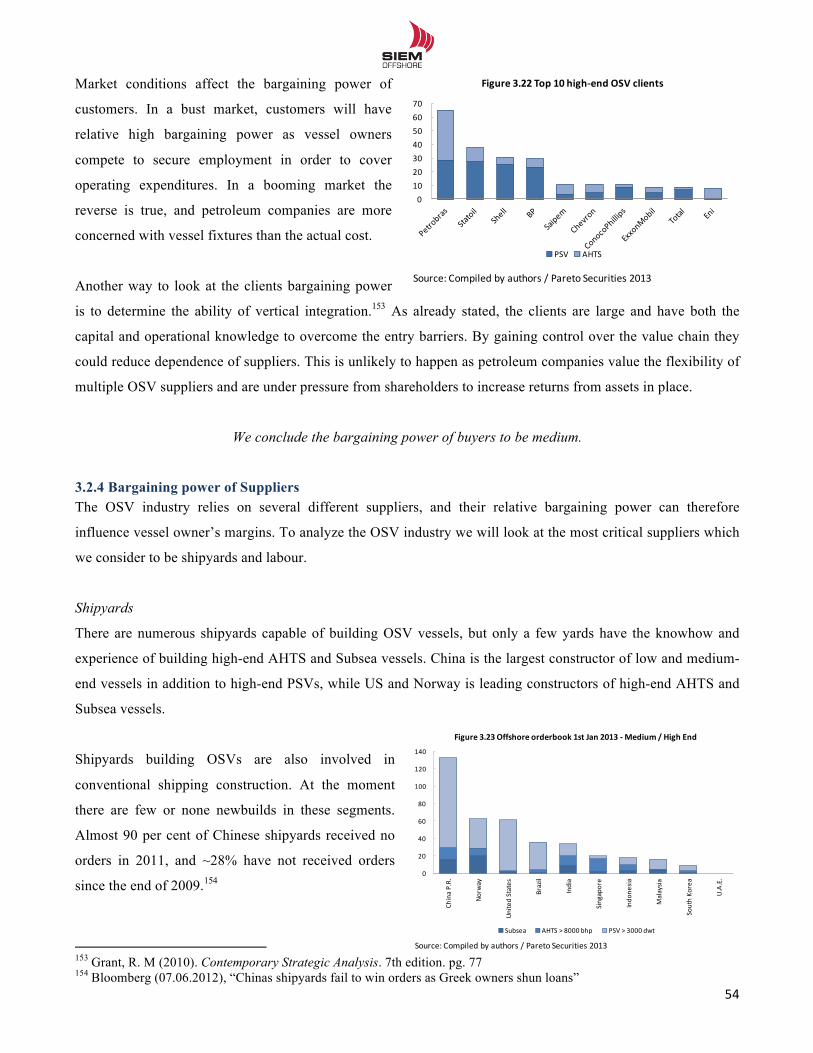
!!
54!!
Market conditions affect the bargaining power of
customers. In a bust market, customers will have
relative high bargaining power as vessel owners
compete to secure employment in order to cover
operating expenditures. In a booming market the
reverse is true, and petroleum companies are more
concerned with vessel fixtures than the actual cost.
Another way to look at the clients bargaining power
is to determine the ability of vertical integration.153 As already stated, the clients are large and have both the
capital and operational knowledge to overcome the entry barriers. By gaining control over the value chain they
could reduce dependence of suppliers. This is unlikely to happen as petroleum companies value the flexibility of
multiple OSV suppliers and are under pressure from shareholders to increase returns from assets in place.
We conclude the bargaining power of buyers to be medium.
3.2.4 Bargaining power of Suppliers The OSV industry relies on several different suppliers, and their relative bargaining power can therefore
influence vessel owner’s margins. To analyze the OSV industry we will look at the most critical suppliers which
we consider to be shipyards and labour.
Shipyards
There are numerous shipyards capable of building OSV vessels, but only a few yards have the knowhow and
experience of building high-end AHTS and Subsea vessels. China is the largest constructor of low and medium-
end vessels in addition to high-end PSVs, while US and Norway is leading constructors of high-end AHTS and
Subsea vessels.
Shipyards building OSVs are also involved in
conventional shipping construction. At the moment
there are few or none newbuilds in these segments.
Almost 90 per cent of Chinese shipyards received no
orders in 2011, and ~28% have not received orders
since the end of 2009.154
!!!!!!!!!!!!!!!!!!!!!!!!!!!!!!!!!!!!!!!!!!!!!!!!!!!!!!!!!!!!!153 Grant, R. M (2010). Contemporary Strategic Analysis. 7th edition. pg. 77 154 Bloomberg (07.06.2012), “Chinas shipyards fail to win orders as Greek owners shun loans”
010203040506070
Figure'3.22'Top'10'high1end'OSV'clients
PSV AHTS
Source:5Compiled by5authors /5Pareto Securities 2013
0
20
40
60
80
100
120
140
China,P.R.
Norw
ay
Unite
d,States
Brazil
India
Singapore
Indo
nesia
Malaysia
South,Ko
rea
U.A.E.
Figure'3.23'Offshore'orderbook'1st'Jan'2013'9 Medium'/'High'End
Subsea AHTS,>,8000,bhp PSV,>,3000,dwt
Source:,Compiled by,authors /,Pareto Securities 2013
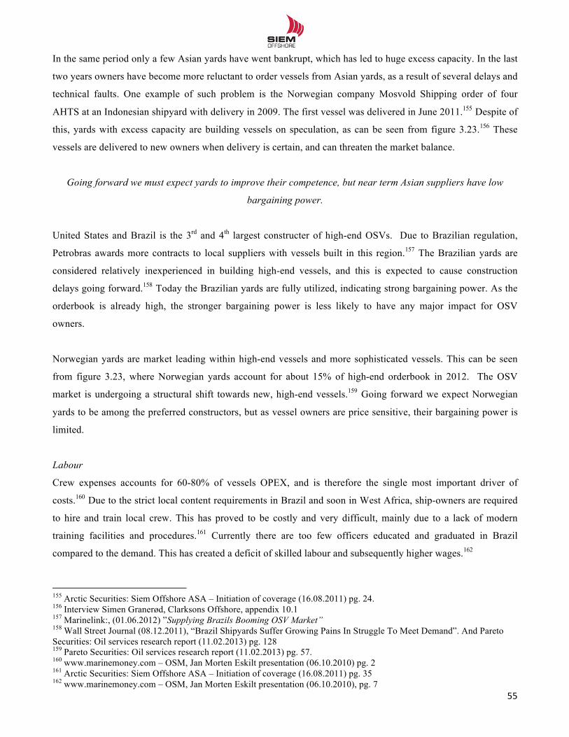
!!
55!!
In the same period only a few Asian yards have went bankrupt, which has led to huge excess capacity. In the last
two years owners have become more reluctant to order vessels from Asian yards, as a result of several delays and
technical faults. One example of such problem is the Norwegian company Mosvold Shipping order of four
AHTS at an Indonesian shipyard with delivery in 2009. The first vessel was delivered in June 2011.155 Despite of
this, yards with excess capacity are building vessels on speculation, as can be seen from figure 3.23.156 These
vessels are delivered to new owners when delivery is certain, and can threaten the market balance.
Going forward we must expect yards to improve their competence, but near term Asian suppliers have low
bargaining power.
United States and Brazil is the 3rd and 4th largest constructer of high-end OSVs. Due to Brazilian regulation,
Petrobras awards more contracts to local suppliers with vessels built in this region.157 The Brazilian yards are
considered relatively inexperienced in building high-end vessels, and this is expected to cause construction
delays going forward.158 Today the Brazilian yards are fully utilized, indicating strong bargaining power. As the
orderbook is already high, the stronger bargaining power is less likely to have any major impact for OSV
owners.
Norwegian yards are market leading within high-end vessels and more sophisticated vessels. This can be seen
from figure 3.23, where Norwegian yards account for about 15% of high-end orderbook in 2012. The OSV
market is undergoing a structural shift towards new, high-end vessels.159 Going forward we expect Norwegian
yards to be among the preferred constructors, but as vessel owners are price sensitive, their bargaining power is
limited.
Labour
Crew expenses accounts for 60-80% of vessels OPEX, and is therefore the single most important driver of
costs.160 Due to the strict local content requirements in Brazil and soon in West Africa, ship-owners are required
to hire and train local crew. This has proved to be costly and very difficult, mainly due to a lack of modern
training facilities and procedures.161 Currently there are too few officers educated and graduated in Brazil
compared to the demand. This has created a deficit of skilled labour and subsequently higher wages.162
!!!!!!!!!!!!!!!!!!!!!!!!!!!!!!!!!!!!!!!!!!!!!!!!!!!!!!!!!!!!!155 Arctic Securities: Siem Offshore ASA – Initiation of coverage (16.08.2011) pg. 24. 156 Interview Simen Granerød, Clarksons Offshore, appendix 10.1 157 Marinelink:, (01.06.2012) ”Supplying Brazils Booming OSV Market” 158 Wall Street Journal (08.12.2011), “Brazil Shipyards Suffer Growing Pains In Struggle To Meet Demand”. And Pareto Securities: Oil services research report (11.02.2013) pg. 128 159 Pareto Securities: Oil services research report (11.02.2013) pg. 57. 160 www.marinemoney.com – OSM, Jan Morten Eskilt presentation (06.10.2010) pg. 2 161 Arctic Securities: Siem Offshore ASA – Initiation of coverage (16.08.2011) pg. 35 162 www.marinemoney.com – OSM, Jan Morten Eskilt presentation (06.10.2010), pg. 7
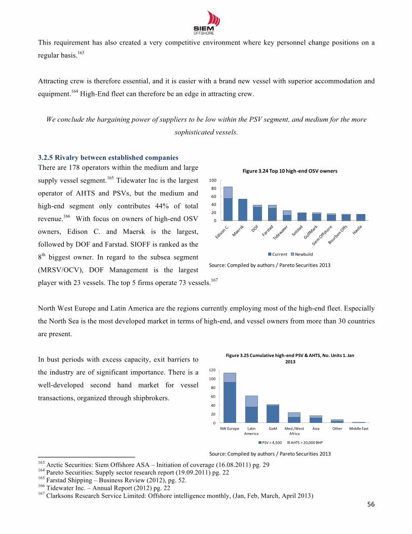
!!
56!!
This requirement has also created a very competitive environment where key personnel change positions on a
regular basis.163
Attracting crew is therefore essential, and it is easier with a brand new vessel with superior accommodation and
equipment.164 High-End fleet can therefore be an edge in attracting crew.
We conclude the bargaining power of suppliers to be low within the PSV segment, and medium for the more
sophisticated vessels.
3.2.5 Rivalry between established companies There are 178 operators within the medium and large
supply vessel segment.165 Tidewater Inc is the largest
operator of AHTS and PSVs, but the medium and
high-end segment only contributes 44% of total
revenue.166 With focus on owners of high-end OSV
owners, Edison C. and Maersk is the largest,
followed by DOF and Farstad. SIOFF is ranked as the
8th biggest owner. In regard to the subsea segment
(MRSV/OCV), DOF Management is the largest
player with 23 vessels. The top 5 firms operate 73 vessels.167
North West Europe and Latin America are the regions currently employing most of the high-end fleet. Especially
the North Sea is the most developed market in terms of high-end, and vessel owners from more than 30 countries
are present.
In bust periods with excess capacity, exit barriers to
the industry are of significant importance. There is a
well-developed second hand market for vessel
transactions, organized through shipbrokers.
!!!!!!!!!!!!!!!!!!!!!!!!!!!!!!!!!!!!!!!!!!!!!!!!!!!!!!!!!!!!!163 Arctic Securities: Siem Offshore ASA – Initiation of coverage (16.08.2011) pg. 29 164 Pareto Securities: Supply sector research report (19.09.2011) pg. 22 165 Farstad Shipping – Business Review (2012), pg. 52. 166 Tidewater Inc. – Annual Report (2012) pg. 22 167 Clarksons Research Service Limited: Offshore intelligence monthly, (Jan, Feb, March, April 2013)
Source:(Compiled by(authors /(Pareto Securities 2013
0
20
40
60
80
100
Figure'3.24'Top'10'high2end'OSV'owners
Current Newbuild
Source:(Compiled by(authors /(Pareto Securities 2013
0
20
40
60
80
100
120
NW(Europe Latin(America
GoM Med./West(Africa
Asia Other Middle(East
Figure'3.25'Cumulative'high3end'PSV'&'AHTS,'No.'Units'1.'Jan'2013
PSV(>(4,500 AHTS(>(20,000(BHP
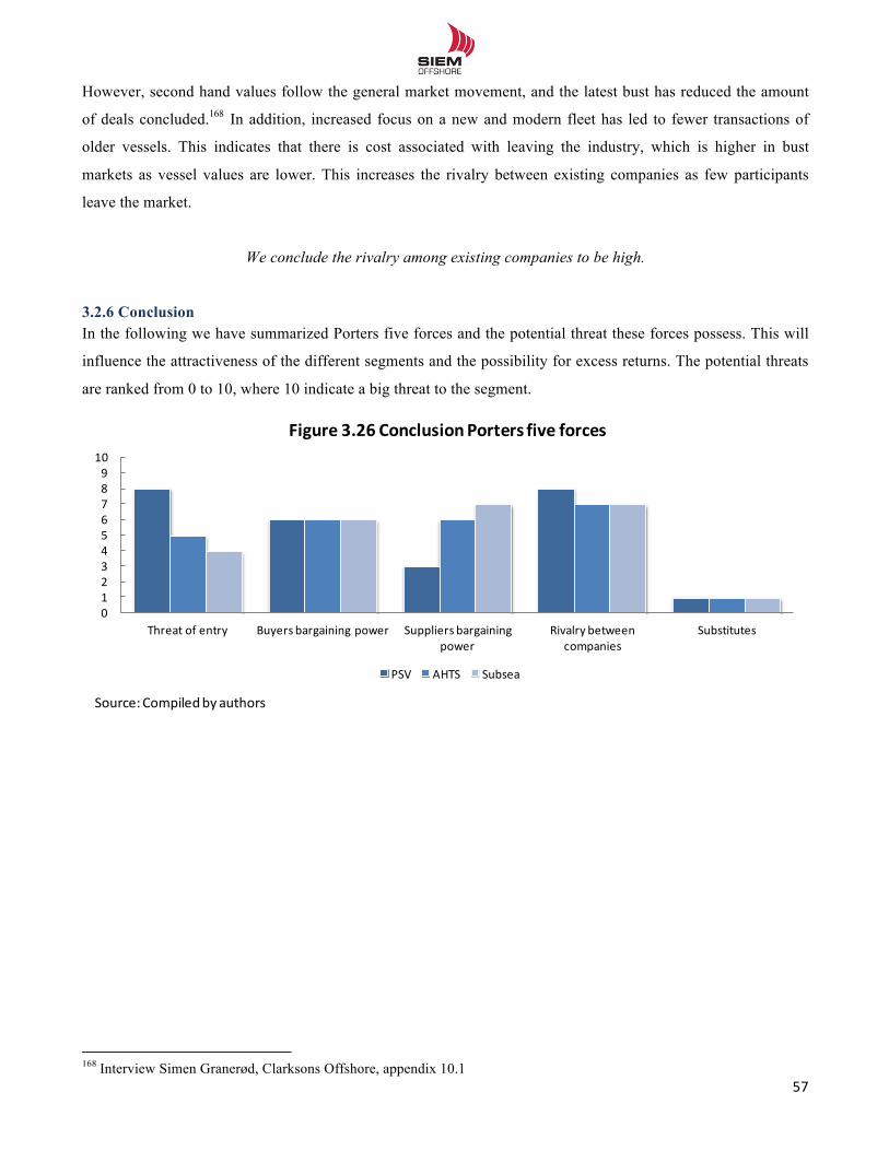
!!
57!!
However, second hand values follow the general market movement, and the latest bust has reduced the amount
of deals concluded.168 In addition, increased focus on a new and modern fleet has led to fewer transactions of
older vessels. This indicates that there is cost associated with leaving the industry, which is higher in bust
markets as vessel values are lower. This increases the rivalry between existing companies as few participants
leave the market.
We conclude the rivalry among existing companies to be high.
3.2.6 Conclusion In the following we have summarized Porters five forces and the potential threat these forces possess. This will
influence the attractiveness of the different segments and the possibility for excess returns. The potential threats
are ranked from 0 to 10, where 10 indicate a big threat to the segment.
!
!
!
!
!
!
!
!!!!!!!!!!!!!!!!!!!!!!!!!!!!!!!!!!!!!!!!!!!!!!!!!!!!!!!!!!!!!168 Interview Simen Granerød, Clarksons Offshore, appendix 10.1
Source:(Compiledby(authors
012345678910
Threat(of(entry Buyers(bargaining(power Suppliers(bargaining(power
Rivalry(between(companies
Substitutes
Figure'3.26'Conclusion'Porters'five'forces
PSV AHTS Subsea
!!
58!!
3.2.7 Market outlook for the OSV industry Porter’s five forces give us an implication of how the industry attractiveness is today. In order to forecast
profitability in the long run, we need to predict whether there will be potential structural changes within the OSV
industry.
Today, there are few (or none) companies which own only high-end vessels. Due to financial constraints and
capacity at yards, we do not believe there is a climate for M&A activity. Few companies are likely to leave the
market as a result of currently high exit barriers. As a result of low M&A activity, we forecast that the number of
companies within the OSV industry will remain high, and the rivalry between companies will be unchanged. We
also believe there will be higher entry barriers in terms of higher capital requirements as a result of demand after
more sophisticated vessels.
Due to the historical fluctuations in the industry, we expect companies in the future to diversify their fleet
composition to be able to deliver a broader set of services. An example of this is SIOFFs focus towards the
renewable energy business with one dedicated newbuilding. It is also likely to see companies expand their
business towards new geographical areas, to meet new demand trends. There are many players in the industry,
and therefore difficult for SIOFF to increase their market share significantly within the next 5-10 years. As a
result of these findings, we do not expect any structural changes in the OSV industry which will change the
industry profitability in the long run.
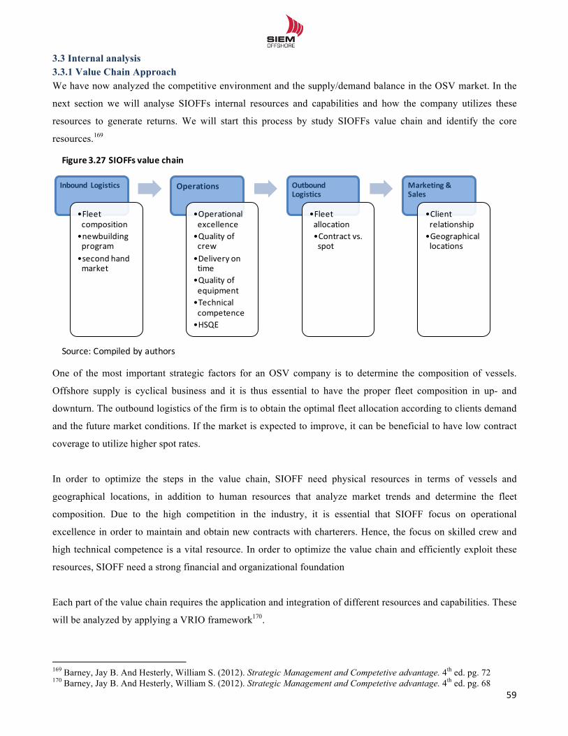
!!
59!!
3.3 Internal analysis 3.3.1 Value Chain Approach We have now analyzed the competitive environment and the supply/demand balance in the OSV market. In the
next section we will analyse SIOFFs internal resources and capabilities and how the company utilizes these
resources to generate returns. We will start this process by study SIOFFs value chain and identify the core
resources.169
One of the most important strategic factors for an OSV company is to determine the composition of vessels.
Offshore supply is cyclical business and it is thus essential to have the proper fleet composition in up- and
downturn. The outbound logistics of the firm is to obtain the optimal fleet allocation according to clients demand
and the future market conditions. If the market is expected to improve, it can be beneficial to have low contract
coverage to utilize higher spot rates.
In order to optimize the steps in the value chain, SIOFF need physical resources in terms of vessels and
geographical locations, in addition to human resources that analyze market trends and determine the fleet
composition. Due to the high competition in the industry, it is essential that SIOFF focus on operational
excellence in order to maintain and obtain new contracts with charterers. Hence, the focus on skilled crew and
high technical competence is a vital resource. In order to optimize the value chain and efficiently exploit these
resources, SIOFF need a strong financial and organizational foundation
Each part of the value chain requires the application and integration of different resources and capabilities. These
will be analyzed by applying a VRIO framework170.
!!!!!!!!!!!!!!!!!!!!!!!!!!!!!!!!!!!!!!!!!!!!!!!!!!!!!!!!!!!!!169 Barney, Jay B. And Hesterly, William S. (2012). Strategic Management and Competetive advantage. 4th ed. pg. 72 170 Barney, Jay B. And Hesterly, William S. (2012). Strategic Management and Competetive advantage. 4th ed. pg. 68
Inbound Logistics
•Fleetcomposition•newbuilding2program•second2hand2market
Operations
•Operationalexcellence•Quality of2crew•Delivery ontime•Quality of2equipment•Technicalcompetence•HSQE
OutboundLogistics
•Fleetallocation•Contract2vs.2spot
Marketing4&4Sales
•Clientrelationship•Geographical2locations
Source:2Compiled by2authors
Figure3.274SIOFFs value chain
!!
60!!
3.3.2 VRIO Based on the different steps of the value chain we will analyze physical, human, financial, and organizational
resources in order to determine potential competitive advantage.
3.3.2.1 Physical resources The fleet and competitive advantage
SIOFFs fleet is the main source of revenue. As previously mentioned, SIOFF has a fleet of modern, high-end
vessels, the youngest among peers. This has proven valuable as demand from petroleum companies has shifted
towards modern vessels suitable for deepwater and harsh environment.171 For charterers, like Statoil and
Petrobras, it is extremely important not to be associated with environmental damages, and therefore they
demand modern vessels with high quality of operations. The modern fleet of high-end vessels is therefore a
competitive advantage and put the company in a position for further growth.
SIOFF has pursued a growth strategy, by ordering multiple vessels at the same time, with the same
specifications. In this way they have been able to obtain lower construction price.172 After delivery, identical
vessels allows for greater economies of scale in crew training, inventory/spare part management and vessel
repair. The whole fleet of AHTS vessels is of the same class, and the same is the case for the OSCV under
construction.
The modern fleet of similar vessels that SIOFF possess is rare among OSV companies. Due to low financial
gearing relative to peers, the company will have the opportunity to maintain this advantage in near future.
Construction time and limited yard capacity will make other companies lag a couple of years after SIOFF.173
This analysis suggests that the fleet is highly valuable and a strength for SIOFF. The modern fleet and fleet
composition is rare, making it a temporary competitive advantage.
!!!!!!!!!!!!!!!!!!!!!!!!!!!!!!!!!!!!!!!!!!!!!!!!!!!!!!!!!!!!!171 Siem Offshore – (Q4 Report) pg. 21 172 Siem Offshore – Annual Report (2006), pg. 6: approx NOK 3.2 billion for first 6 vessels, approx USD 80m per vessel. Compared with historical values in Fearnley foil pg. 49, is seems that SIOFF managed to achieve a lower construction price. 173 Ref. Porters Five Forces
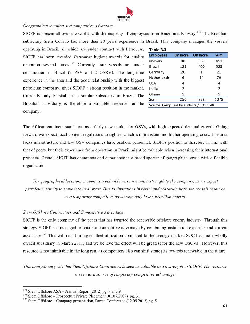
!!
61!!
Geographical location and competitive advantage
SIOFF is present all over the world, with the majority of employees from Brazil and Norway.174 The Brazilian
subsidiary Siem Consub has more than 20 years experience in Brazil. This company manages the vessels
operating in Brazil, all which are under contract with Petrobras.
SIOFF has been awarded Petrobras highest awards for quality
operation several times.175 Currently four vessels are under
construction in Brazil (2 PSV and 2 OSRV). The long-time
experience in the area and the good relationship with the biggest
petroleum company, gives SIOFF a strong position in the market.
Currently only Farstad has a similar subsidiary in Brazil. The
Brazilian subsidiary is therefore a valuable resource for the
company.
The African continent stands out as a fairly new market for OSVs, with high expected demand growth. Going
forward we expect local content regulations to tighten which will translate into higher operating costs. The area
lacks infrastructure and few OSV companies have onshore personnel. SIOFFs position is therefore in line with
that of peers, but their experience from operation in Brazil might be valuable when increasing their international
presence. Overall SIOFF has operations and experience in a broad specter of geographical areas with a flexible
organization.
The geographical locations is seen as a valuable resource and a strength to the company, as we expect
petroleum activity to move into new areas. Due to limitations in rarity and cost-to-imitate, we see this resource
as a temporary competitive advantage only in the Brazilian market.
Siem Offshore Contractors and Competetive Advantage
SIOFF is the only company of the peers that has targeted the renewable offshore energy industry. Through this
strategy SIOFF has managed to obtain a competitive advantage by combining installation expertise and current
asset base.176 This will result in higher fleet utilization compared to the average market. SOC became a wholly
owned subsidiary in March 2011, and we believe the effect will be greatest for the new OSCVs . However, this
resource is not inimitable in the long run, as competitors also can shift strategies towards renewable in the future.
This analysis suggests that Siem Offshore Contractors is seen as valuable and a strength to SIOFF. The resource
is seen as a source of temporary competitive advantage.
!!!!!!!!!!!!!!!!!!!!!!!!!!!!!!!!!!!!!!!!!!!!!!!!!!!!!!!!!!!!!174 Siem Offshore ASA – Annual Report (2012) pg. 8 and 9. 175 Siem Offshore – Prospectus: Private Placement (01.07.2009) pg. 31 176 Siem Offshore – Company presentation, Pareto Conference (12.09.2012) pg. 5
Table&3.3Employees Onshore Offshore SumNorway 88 363 451Brazil 125 400 525Germany 20 1 21Netherlands 6 64 70USA 4 4India 2 2Ghana 5 5Sum 250 828 1078Source:CCompi ledCbyCauthors C/CSIOFFCAR
!!
62!!
3.3.2.2 Individual and Human Resources The human resources include training, experience, and insight of individual managers and workers in the firm. In
this section we will analyze crew and executive managers
Crew
The knowledge and the experience of the crew is a vital resource for SIOFF. With the already mentioned demand
after quality of operations from charterers, the crew plays an important role in this matter. It is therefore essential
for SIOFF to have a high quality of training of employees. SIOFF has a long-term collaboration with Offshore
Simulator Centre and Ålesund University College in order to achieve an optimal training of crew.177 This is part
of SIOFFs plan for a comprehensive and systematic personnel and training development.178 As mentioned in
Porters, a new and modern fleet will attract experienced crew. This is beneficial for SIOFF as they have one of
the most modern fleets among competitors. Another attracting factor is zero work related accidents from 2009-
2012.179
There is nothing to suggest that SIOFF do not fully exploit their qualified crew. However, this is in line with
competitors. There is progressively more focus on training and safety among competitors, which gives the
companies an incentive to invest more in their sailors.180 It is believed that those who do not seek to obtain highly
qualified personnel will lose market shares in the long run.
This analysis suggests that the crew is valuable and a strength for SIOFF, but due to limitations in rarity and
cost-to-imitate, we see the resource as a competitive parity.
Management and Board of Directors
The board of directors has been very stable since the beginning in 2006.181 This underpins a long-term focus, and
gives management time to comply with their strategy. The current CEO has been with the company for the entire
period and there have only been minor changes in the management.182 As described in section 2.5, the
management team has relevant experience from related industry through former employments in other maritime
companies. The Norwegian maritime cluster is small, and this indicates good influence towards Norwegian
yards, lenders and charterers. With the top management skills and expertise, SIOFF is able to exploit
opportunities within the industry. In the following we will analyze how management has performed in order to
determine a potential competitive advantage.
!!!!!!!!!!!!!!!!!!!!!!!!!!!!!!!!!!!!!!!!!!!!!!!!!!!!!!!!!!!!!177 Siem Offshore ASA – Annual Report (2011) pg. 14 178 http://www.skipsrevyen.no/nyheter/11020.html 179 Siem Offshore ASA – Annual Reports (2009-2012) 180 Annual reports 2012: Havila pg. 22, DOF pg. 27, Farstad pg. 6, Solstad pg. 19. 181 Siem Offshore – Annual Reports (2007-2012) board of directors report 182 www.siemoffshore.com - Management
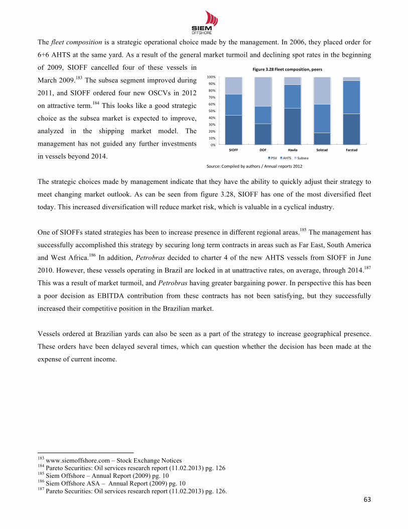
!!
63!!
The fleet composition is a strategic operational choice made by the management. In 2006, they placed order for
6+6 AHTS at the same yard. As a result of the general market turmoil and declining spot rates in the beginning
of 2009, SIOFF cancelled four of these vessels in
March 2009.183 The subsea segment improved during
2011, and SIOFF ordered four new OSCVs in 2012
on attractive term.184 This looks like a good strategic
choice as the subsea market is expected to improve,
analyzed in the shipping market model. The
management has not guided any further investments
in vessels beyond 2014.
The strategic choices made by management indicate that they have the ability to quickly adjust their strategy to
meet changing market outlook. As can be seen from figure 3.28, SIOFF has one of the most diversified fleet
today. This increased diversification will reduce market risk, which is valuable in a cyclical industry.
One of SIOFFs stated strategies has been to increase presence in different regional areas.185 The management has
successfully accomplished this strategy by securing long term contracts in areas such as Far East, South America
and West Africa.186 In addition, Petrobras decided to charter 4 of the new AHTS vessels from SIOFF in June
2010. However, these vessels operating in Brazil are locked in at unattractive rates, on average, through 2014.187
This was a result of market turmoil, and Petrobras having greater bargaining power. In perspective this has been
a poor decision as EBITDA contribution from these contracts has not been satisfying, but they successfully
increased their competitive position in the Brazilian market.
Vessels ordered at Brazilian yards can also be seen as a part of the strategy to increase geographical presence.
These orders have been delayed several times, which can question whether the decision has been made at the
expense of current income.
!!!!!!!!!!!!!!!!!!!!!!!!!!!!!!!!!!!!!!!!!!!!!!!!!!!!!!!!!!!!!183 www.siemoffshore.com – Stock Exchange Notices 184 Pareto Securities: Oil services research report (11.02.2013) pg. 126 185 Siem Offshore – Annual Report (2009) pg. 10 186 Siem Offshore ASA – Annual Report (2009) pg. 10 187 Pareto Securities: Oil services research report (11.02.2013) pg. 126.
Source:(Compiled by(authors /(Annual reports 2012
0%
10%
20%
30%
40%
50%
60%
70%
80%
90%
100%
SIOFF DOF Havila Solstad Farstad
Figure33.283Fleet3composition,3peers
PSV AHTS Subsea
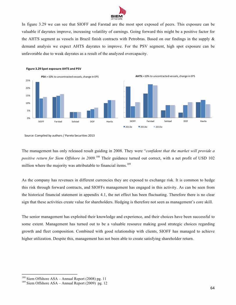
!!
64!!
In figure 3.29 we can see that SIOFF and Farstad are the most spot exposed of peers. This exposure can be
valuable if dayrates improve, increasing volatility of earnings. Going forward this might be a positive factor for
the AHTS segment as vessels in Brazil finish contracts with Petrobras. Based on our findings in the supply &
demand analysis we expect AHTS dayrates to improve. For the PSV segment, high spot exposure can be
unfavorable due to weak dayrates as a result of the analyzed overcapacity.
The management has only released result guiding in 2008. They were “confident that the market will provide a
positive return for Siem Offshore in 2009.188 Their guidance turned out correct, with a net profit of USD 102
million where the majority was attributable to financial items.189
As the company has revenues in different currencies they are exposed to exchange risk. It is common to hedge
this risk through forward contracts, and SIOFFs management has engaged in this activity. As can be seen from
the historical financial statement in appendix 4.1, the net effect has been fluctuating. Therefore there is no clear
sign that these activities create value for shareholders. Hedging is therefore not seen as management’s core skill.
The senior management has exploited their knowledge and experience, and their choices have been successful to
some extent. Management has turned out to be a valuable resource making good strategic choices regarding
growth and fleet composition. Combined with good relationship with clients, SIOFF has managed to achieve
higher utilization. Despite this, management has not been able to create satisfying shareholder return.
!!!!!!!!!!!!!!!!!!!!!!!!!!!!!!!!!!!!!!!!!!!!!!!!!!!!!!!!!!!!!188 Siem Offshore ASA – Annual Report (2008) pg. 11 189 Siem Offshore ASA – Annual Report (2009) pg. 12
0%
5%
10%
15%
20%
25%
30%
35%
SIOFF Farstad Solstad DOF Havila
AHTS:&+10%7to7uncontracted7vessels,7change7in7EPS
2013e 2014e 2015e
0%
5%
10%
15%
20%
25%
SIOFF Farstad Solstad DOF Havila
PSV:&+10%7to7uncontracted7vessels,7change7in7EPS
Source:7Compiled by7authors /7Pareto Securities 2013
Figure 3.29&Spot&exposure AHTS&and&PSV
!!
65!!
SIOFF is not the only company with experienced management, and it is too early to state whether the
management represent a competitive advantage. Many of the peers have management which has worked together
for a longer period of time.190 In addition, management is a tangible asset which the firm does not control.
The management is a highly valuable resource for SIOFF, but due to limitations in rarity and imitations, we
consider them as a competitive parity.
3.3.2.3 Financial resources In 2012, the debt ratio was 58%, retained earnings were USD 17 millions, and cash amounted to USD 107
millions.191 As can be seen from the financial analysis, SIOFF and Farstad are the least leveraged firms. Despite
SIOFFs aggressive newbuilding program, growth has been funded through several channels. One example is the
private placement in July 2009, were gross proceeds of NOK 900 millions where raised.192 All current newbuilds
are likely to be funded through export credit facilities and available cash, including the recent bond issue of NOK
600 million in February 2013.193 Due to the low leverage, SIOFF may be in a good financial position to future
growth.
SIOFF has been able to exploit different sources of funding, which explain the current strong financial position.
However, these financial resources are neither rare nor inimitable among competitors.
The financial resources are valuable and characterized as a competitive parity.
3.3.2.4 Organizational and combined resources The organizational resources of a company are an attribute of groups of individuals and includes among other
culture and reputation, informal relationships within the firm and towards the environment, planning, controlling
and coordinating systems.194
SIOFF is the youngest company among peers, but has already managed to be awarded Petrobras highest awards
for quality operations.195 This strengthens SIOFFs brand and reputation, which is a valuable source to obtaining
new contracts, attract qualified labor and retain key executive management.
!!!!!!!!!!!!!!!!!!!!!!!!!!!!!!!!!!!!!!!!!!!!!!!!!!!!!!!!!!!!!190 www.farstad.com – corporate management, www.dof.no – the management, Solstad Annual Report 2012 pg. 17, Havila Annual Report 2012 pg. 8 191 Siem Offshore ASA – Annual Report (2012 ), pg. 24-25 192 www.siemoffshore.com – Stock Exchange Notice 193 Pareto Securities: Oil services research report (11.02.2013), pg.128 194 Barney, Jay B. And Hesterly, William S. (2012). Strategic Management and Competetive advantage. 4th ed. pg. 67. 195 Siem Offshore ASA – Prospectus: Private Placement (01.07.2009), pg. 31
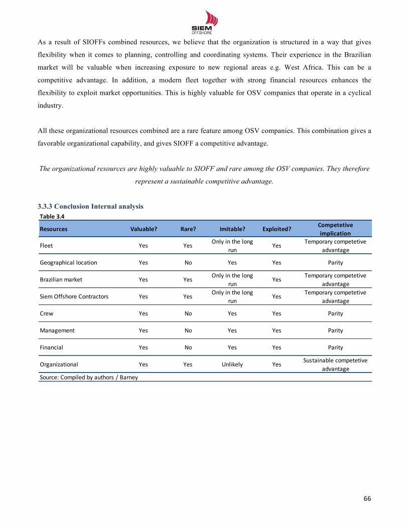
!!
66!!
As a result of SIOFFs combined resources, we believe that the organization is structured in a way that gives
flexibility when it comes to planning, controlling and coordinating systems. Their experience in the Brazilian
market will be valuable when increasing exposure to new regional areas e.g. West Africa. This can be a
competitive advantage. In addition, a modern fleet together with strong financial resources enhances the
flexibility to exploit market opportunities. This is highly valuable for OSV companies that operate in a cyclical
industry.
All these organizational resources combined are a rare feature among OSV companies. This combination gives a
favorable organizational capability, and gives SIOFF a competitive advantage.
The organizational resources are highly valuable to SIOFF and rare among the OSV companies. They therefore
represent a sustainable competitive advantage.
3.3.3 Conclusion Internal analysis
Table&3.4
Resources Valuable? Rare? Imitable? Exploited? Competetive&&&&&implication&&&
Fleet Yes Yes Only*in*the*long*run
Yes Temporary*competetive*advantage
Geographical*location Yes No Yes Yes Parity
Brazilian*market Yes Yes Only*in*the*long*run
Yes Temporary*competetive*advantage
Siem*Offshore*Contractors Yes Yes Only*in*the*long*run
Yes Temporary*competetive*advantage
Crew Yes No Yes Yes Parity
Management Yes No Yes Yes Parity
Financial Yes No Yes Yes Parity
Organizational Yes Yes Unlikely Yes Sustainable*competetive*advantage
Source:*Compiled*by*authors*/*Barney
!!
67!!
4.0 Financial Statement Analysis
In order to forecast SIOFFs future cash flow, it is essential to get an understanding of the historical performance.
By thoroughly analyzing financial statements, we can document how the company has created value, and how it
compares with the peer group. Understanding how the most important value drivers have developed in the past
will help us make more reliable estimates of future cash flow.196 The customers such as Petrobras and Statoil
have often long term relationship with the company. The financial performance and profitability is therefore not
only of importance for the shareholders but also many of the stakeholders.197
SIOFFs performance will be benchmarked against a selected peer group based on operational criteria. The
following financial analysis is based on annual reports from SIOFF and the peers between 2006 and 2012. As
described in part 2.11, a typical business cycle for the OSV industry is 8-10 years. This would be a desirable
number of years to analyze, but since SIOFF was established in July 2005, we have only used annual reports
from 2006. We do not use figures from 2005 since we do not have the aggregated number for the entire year, and
therefore cannot compute key financial ratios. However we consider a 7 year historical analysis adequate in order
to understand SIOFFs historical performance in context with the OSV industry.
First we will reorganize the company´s financial statements by separating operating items from non-operating
items, interest bearing assets and interest bearing liabilities. Next we will analyze the company´s historical
performance by different key ratios. Together with the strategic analysis, this will be important input to the
forecasting. The reformulated statements for SIOFF and peers can be seen in appendix 4.1.
!!!!!!!!!!!!!!!!!!!!!!!!!!!!!!!!!!!!!!!!!!!!!!!!!!!!!!!!!!!!!196 Koller,T. Goedhart,M. and Wessels,D. (2010) - Valuation: pg. 107. 197 Plenborg & Petersen (2012) – Financial Statement Analysis pg. 93.
!!
68!!
4.1 Rebalancing financial statements for analytical purpose 4.1.2 The analytical income statement Operating earnings is a key performance measure, as it shows a firm´s profit from its core business regardless of
how it is financed.198 We have therefore classified items according to their relation with the core business. We
have calculated the operating result as NOPAT (Net Operating Profit After Tax). The following reclassifications
have been conducted in the income statement:
- In accordance with the delimitation, we have deducted the results from the associated company Overseas
Drilling Ltd and added the result to results from non-core operations.
- Since the financial statement does not distinguish between tax on operations and tax on financial items,
we need to estimate them separately.199 This is done by calculating the tax shield from net financial
expenses. Since SIOFF operates in several countries with different tax rates, we have chosen to use the
effective tax rate each year.
- Results from associated companies are classified as core operations, as this is results from the vessel Big
Orange and subordinated activity in the Brazilian subsidiary.
- The item gains/loss from sales of asset is characterized as core operations, as historical years have shown
that they continuously aim to have the optimal fleet composition by purchase and sale of vessels. It is
important to highlight that SIOFF does not speculate in asset play200, and these gains and losses are a
result of the core business.
- It can be discussed whether to classify interest rate derivatives and currency exchange forward contracts
as operational or financial items. However, the income statement does not separate in this way, which
makes it difficult to divide the item in practice. As a result, all operating and finance hedges are regarded
as being financial decision.201 Even though different hedging strategies are part of the business, this is
not where the management of SIOFF has it core competence and create value for the shareholders. These
items are therefore characterized as being part of the non-core business.202
!!!!!!!!!!!!!!!!!!!!!!!!!!!!!!!!!!!!!!!!!!!!!!!!!!!!!!!!!!!!!198 Plenborg & Petersen (2012) – Financial Statement Analysis pg 73 199 Plenborg & Petersen (2012) – Financial Statement Analysis pg. 76. 200 Asset Play: Sell newbuilding orders in the second hand market before the vessel is delivered. 201 Plenborg & Petersen (2012) – Financial Statement Analysis pg. 78 202 Plenborg & Petersen (2012) – Financial Statement Analysis pg 77
!!
69!!
4.1.3 The analytical balance sheet In the balance sheet we have calculated the invested capital, as the sum of all operating assets less operating
liabilities. These assets are funded by shareholders and lenders, and are thus equal to equity capital plus net
interest bearing debt (NIBD).203 Shareholders and lenders required return is expressed as WACC, which we will
determine in part 7.0. To obtain these figures, the following items are classified as core, non-core or financial
asset.
- The item taxes payable is a result of core activities and thus characterized as operational and included in
working capital.
- The item other short-term receivables include a short-term loan to a shipyard in 2008 and 2009. We
consider this item as part of operations, and thus part of the total assets as loan to shipyard.
- It is difficult to separate cash reserves into operating and excess cash.204 The cash reserves have been
volatile as a result of funding needed for new vessels. For the last three years reserves has been rather
stable. As some of this cash will be used for payment of new vessels, we have therefore classified 50%
as operational, and the remaining 50% as interest bearing assets.
- SIOFF has made an announcement in January that they will explore strategic alternatives for Siem WIS.
The book value of Siem WIS is therefore deducted from the accounting item intangible assets, and
added as interest bearing asset under investments in non-core operations.
- The investment in Overseas Drilling Ltd is deducted from the accounting item investments in associated
companies, and added to investments in non-core operations.
- The item long-term receivables include loan to employees, where the latter is characterized as interest
bearing. We therefore separate these two items.
- Forward currency contracts and Derivative financial instruments are classified as financial, due to the
fact that this is only used as a hedging strategy and it is difficult to segregate the post.
!
!!!!!!!!!!!!!!!!!!!!!!!!!!!!!!!!!!!!!!!!!!!!!!!!!!!!!!!!!!!!!203 NIBD = Interest bearing liabilities – Interest bearing assets 204 Plenborg & Petersen (2012) – Financial Statement Analysis pg. 77.
!!
70!!
4.2 Analysis of historical profitability and performance To analyze the historical performance we will first look at the operational result, and then look at the result
through the owner’s perspective. For this purpose we will use an approach based on the DuPont model, which is
further explained in appendix 4.2. All balance sheet ratios are based on average numbers.
The operational result is created through the core business of the company and is best analyzed through the
measure Return On Invested Capital (ROIC).205 ROIC does not explain whether profitability is driven by an
improved revenue/cost relation or better utilization of capital.206 Therefore we will analyze the sources of value
creation from operational activities by decomposing this measure into profit margin (PM) and turnover rate on
invested capital. The level of ROIC will be analyzed by comparing ROIC with the company´s WACC calculated
in part 7.0.
For the company´s shareholders the ultimate measurement for profitability is Return On Equity (ROE).
Shareholders are left with the profit on the bottom line, and are thus affected by all the company´s financial
positions. This way ROE capture the result from both operational and financial transactions. By decomposing
ROE into Spread and F-Gear, we will analyze the impact of financial leverage on the shareholder value.
In order to analyze trends in the financial data we will use index analysis for both the income statement and
balance sheet. However, index numbers does not reveal the relative size of each item. For this purpose, common
size analysis is more useful. These analysis will help us explain the development in different operational items
and will enable us to identify potential for e.g. better cost or inventory management.207
Throughout the analysis we will compare SIOFFs results with the peer group and thus look at the relative
development of key ratios. This will give a better image of the company´s historical performance. Analysis of
margins, growth rate and return across peer group will be valuable input to the subsequent forecast, as it will help
us position SIOFF in the OSV industry.
!!!!!!!!!!!!!!!!!!!!!!!!!!!!!!!!!!!!!!!!!!!!!!!!!!!!!!!!!!!!!205 Koller,T. Goedhart,M. and Wessels,D. (2010) - Valuation: pg. 163 206 Plenborg & Petersen (2012) – Financial Statement Analysis pg. 107 207 Plenborg & Petersen (2012) – Financial Statement Analysis pg. 112
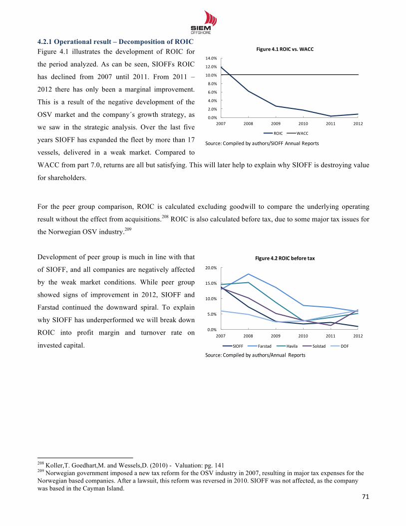
!!
71!!
4.2.1 Operational result – Decomposition of ROIC Figure 4.1 illustrates the development of ROIC for
the period analyzed. As can be seen, SIOFFs ROIC
has declined from 2007 until 2011. From 2011 –
2012 there has only been a marginal improvement.
This is a result of the negative development of the
OSV market and the company´s growth strategy, as
we saw in the strategic analysis. Over the last five
years SIOFF has expanded the fleet by more than 17
vessels, delivered in a weak market. Compared to
WACC from part 7.0, returns are all but satisfying. This will later help to explain why SIOFF is destroying value
for shareholders.
For the peer group comparison, ROIC is calculated excluding goodwill to compare the underlying operating
result without the effect from acquisitions.208 ROIC is also calculated before tax, due to some major tax issues for
the Norwegian OSV industry.209
Development of peer group is much in line with that
of SIOFF, and all companies are negatively affected
by the weak market conditions. While peer group
showed signs of improvement in 2012, SIOFF and
Farstad continued the downward spiral. To explain
why SIOFF has underperformed we will break down
ROIC into profit margin and turnover rate on
invested capital.
!!!!!!!!!!!!!!!!!!!!!!!!!!!!!!!!!!!!!!!!!!!!!!!!!!!!!!!!!!!!!208 Koller,T. Goedhart,M. and Wessels,D. (2010) - Valuation: pg. 141 209 Norwegian government imposed a new tax reform for the OSV industry in 2007, resulting in major tax expenses for the Norwegian based companies. After a lawsuit, this reform was reversed in 2010. SIOFF was not affected, as the company was based in the Cayman Island.
0.0%
2.0%
4.0%
6.0%
8.0%
10.0%
12.0%
14.0%
2007 2008 2009 2010 2011 2012
Figure'4.1'ROIC'vs.'WACC
ROIC WACC
Source:8Compiled by8authors/SIOFF Annual Reports
0.0%
5.0%
10.0%
15.0%
20.0%
2007 2008 2009 2010 2011 2012
FIgure'4.2'ROIC'before'tax
SIOFF Farstad Havila Solstad DOF
Source:=Compiled by=authors/Annual Reports
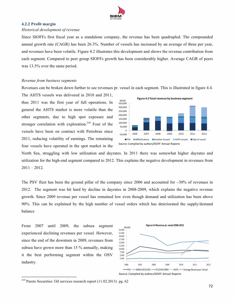
!!
72!!
4.2.2 Profit margin Historical development of revenue
Since SIOFFs first fiscal year as a standalone company, the revenue has been quadrupled. The compounded
annual growth rate (CAGR) has been 26.3%. Number of vessels has increased by an average of three per year,
and revenues have been volatile. Figure 4.2 illustrates this development and shows the revenue contribution from
each segment. Compared to peer group SIOFFs growth has been considerably higher. Average CAGR of peers
was 13.5% over the same period.
Revenue from business segments
Revenues can be broken down further to see revenues pr. vessel in each segment. This is illustrated in figure 4.4.
The AHTS vessels was delivered in 2010 and 2011,
thus 2011 was the first year of full operations. In
general the AHTS market is more volatile than the
other segmnets, due to high spot exposure and
stronger correlation with exploration.210 Four of the
vessels have been on contract with Petrobras since
2011, reducing volatility of earnings. The remaining
four vessels have operated in the spot market in the
North Sea, struggling with low utilization and dayrates. In 2011 there was somewhat higher dayrates and
utilization for the high-end segment compared to 2012. This explains the negative development in revenues from
2011 – 2012.
The PSV fleet has been the ground pillar of the company since 2006 and accounted for ~30% of revenues in
2012. The segment was hit hard by decline in dayrates in 2008-2009, which explains the negative revenue
growth. Since 2009 revenue per vessel has remained low even though demand and utilization has been above
90%. This can be explained by the high number of vessel orders which has deteriorated the supply/demand
balance
From 2007 until 2009, the subsea segment
experienced declining revenues per vessel. However,
since the end of the downturn in 2009, revenues from
subsea have grown more than 15 % annually, making
it the best performing segment within the OSV
industry.
!!!!!!!!!!!!!!!!!!!!!!!!!!!!!!!!!!!!!!!!!!!!!!!!!!!!!!!!!!!!!210 Pareto Securities: Oil services research report (11.02.2013) pg. 62
!50,000
0
50,000
100,000
150,000
200,000
250,000
300,000
350,000
2006 2007 2008 2009 2010 2011 2012
Figure'4.3'Total'revenue'by'business'segment
PSV MRSV/Subsea Brazilian=Vessels AHTS=vessels Sale=of=vessel
Source:=Compiled by=authors/SIOFF Annual Reports
MUSD
!2,500&5,000&7,500&10,000&12,500&15,000&17,500&20,000&22,500&25,000&
2006 2007 2008 2009 2010 2011 2012
Figure'4.4'Revenue'pr.'vessel'200632012
PSV MRSV/OCSV/ISV FCV/FSV/OSRV AHTS Average&Revenue&pr.&Vessel
Source:&Compiled by&authors/SIOFF Annual Reports
MUSD
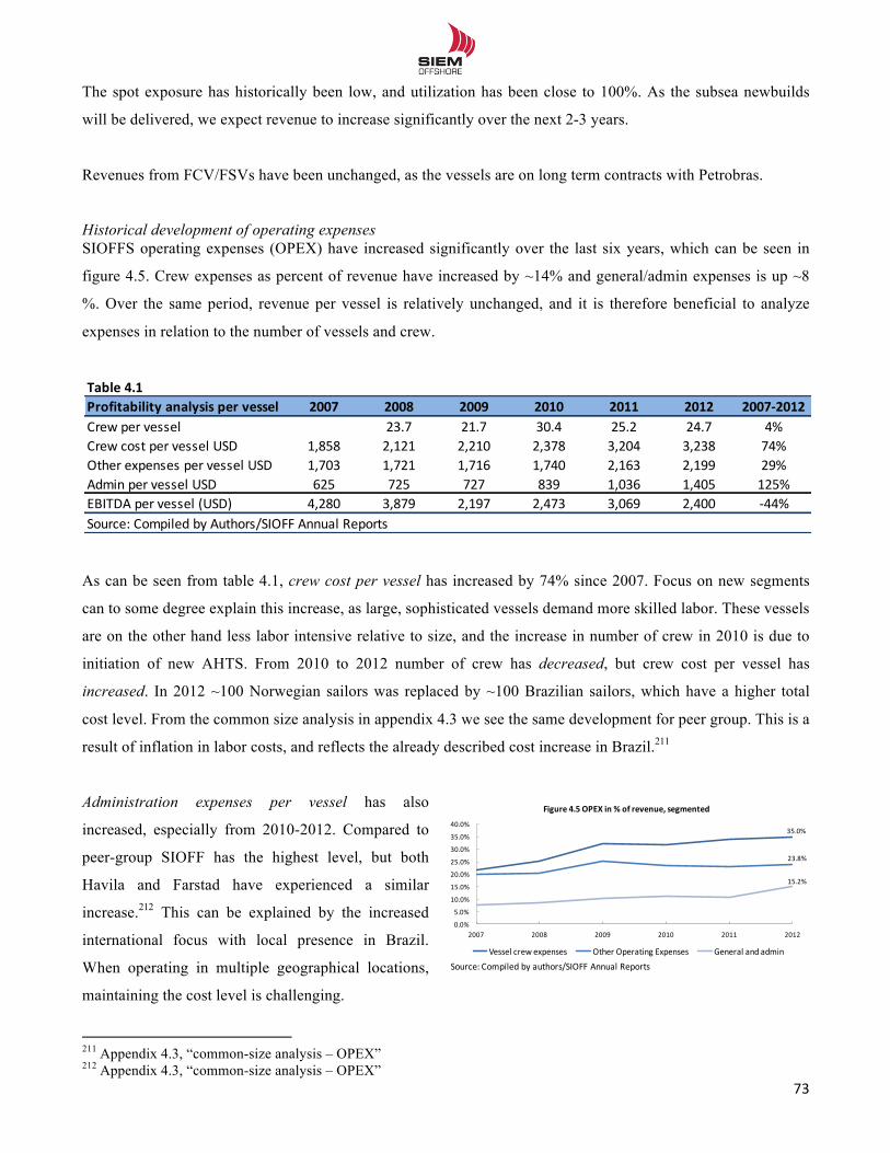
!!
73!!
The spot exposure has historically been low, and utilization has been close to 100%. As the subsea newbuilds
will be delivered, we expect revenue to increase significantly over the next 2-3 years.
Revenues from FCV/FSVs have been unchanged, as the vessels are on long term contracts with Petrobras.
Historical development of operating expenses SIOFFS operating expenses (OPEX) have increased significantly over the last six years, which can be seen in
figure 4.5. Crew expenses as percent of revenue have increased by ~14% and general/admin expenses is up ~8
%. Over the same period, revenue per vessel is relatively unchanged, and it is therefore beneficial to analyze
expenses in relation to the number of vessels and crew.
As can be seen from table 4.1, crew cost per vessel has increased by 74% since 2007. Focus on new segments
can to some degree explain this increase, as large, sophisticated vessels demand more skilled labor. These vessels
are on the other hand less labor intensive relative to size, and the increase in number of crew in 2010 is due to
initiation of new AHTS. From 2010 to 2012 number of crew has decreased, but crew cost per vessel has
increased. In 2012 ~100 Norwegian sailors was replaced by ~100 Brazilian sailors, which have a higher total
cost level. From the common size analysis in appendix 4.3 we see the same development for peer group. This is a
result of inflation in labor costs, and reflects the already described cost increase in Brazil.211
Administration expenses per vessel has also
increased, especially from 2010-2012. Compared to
peer-group SIOFF has the highest level, but both
Havila and Farstad have experienced a similar
increase.212 This can be explained by the increased
international focus with local presence in Brazil.
When operating in multiple geographical locations,
maintaining the cost level is challenging.
!!!!!!!!!!!!!!!!!!!!!!!!!!!!!!!!!!!!!!!!!!!!!!!!!!!!!!!!!!!!!211 Appendix 4.3, “common-size analysis – OPEX” 212 Appendix 4.3, “common-size analysis – OPEX”
Table&4.1Profitability&analysis&per&vessel 2007 2008 2009 2010 2011 2012 2007:2012Crew%per%vessel 23.7 21.7 30.4 25.2 24.7 4%Crew%cost%per%vessel%USD 1,858 2,121 2,210 2,378 3,204 3,238 74%Other%expenses%per%vessel%USD 1,703 1,721 1,716 1,740 2,163 2,199 29%Admin%per%vessel%USD 625 725 727 839 1,036 1,405 125%EBITDA%per%vessel%(USD) 4,280 3,879 2,197 2,473 3,069 2,400 K44%Source:%Compiled%by%Authors/SIOFF%Annual%Reports
35.0%
23.8%
15.2%
0.0%
5.0%
10.0%
15.0%
20.0%
25.0%
30.0%
35.0%
40.0%
2007 2008 2009 2010 2011 2012
Figure'4.5'OPEX'in'%'of'revenue,'segmented
Vessel0crew0expenses Other0Operating0Expenses General0and0admin
Source:0Compiled by0authors/SIOFF Annual Reports
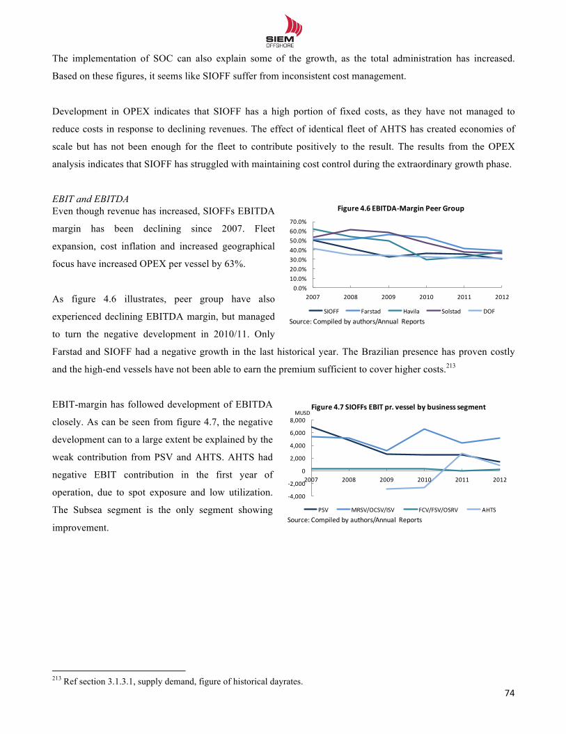
!!
74!!
The implementation of SOC can also explain some of the growth, as the total administration has increased.
Based on these figures, it seems like SIOFF suffer from inconsistent cost management.
Development in OPEX indicates that SIOFF has a high portion of fixed costs, as they have not managed to
reduce costs in response to declining revenues. The effect of identical fleet of AHTS has created economies of
scale but has not been enough for the fleet to contribute positively to the result. The results from the OPEX
analysis indicates that SIOFF has struggled with maintaining cost control during the extraordinary growth phase.
EBIT and EBITDA Even though revenue has increased, SIOFFs EBITDA
margin has been declining since 2007. Fleet
expansion, cost inflation and increased geographical
focus have increased OPEX per vessel by 63%.
As figure 4.6 illustrates, peer group have also
experienced declining EBITDA margin, but managed
to turn the negative development in 2010/11. Only
Farstad and SIOFF had a negative growth in the last historical year. The Brazilian presence has proven costly
and the high-end vessels have not been able to earn the premium sufficient to cover higher costs.213
EBIT-margin has followed development of EBITDA
closely. As can be seen from figure 4.7, the negative
development can to a large extent be explained by the
weak contribution from PSV and AHTS. AHTS had
negative EBIT contribution in the first year of
operation, due to spot exposure and low utilization.
The Subsea segment is the only segment showing
improvement.!!
!
!!!!!!!!!!!!!!!!!!!!!!!!!!!!!!!!!!!!!!!!!!!!!!!!!!!!!!!!!!!!!213 Ref section 3.1.3.1, supply demand, figure of historical dayrates.
0.0%10.0%20.0%30.0%40.0%50.0%60.0%70.0%
2007 2008 2009 2010 2011 2012
Figure'4.6'EBITDA1Margin'Peer'Group
SIOFF Farstad Havila Solstad DOFSource:@Compiled by@authors/Annual Reports
!4,000
!2,000
0
2,000
4,000
6,000
8,000
2007 2008 2009 2010 2011 2012
Figure'4.7'SIOFFs'EBIT'pr.'vessel'by'business'segment
PSV MRSV/OCSV/ISV FCV/FSV/OSRV AHTSSource:>Compiled by>authors/Annual Reports
MUSD
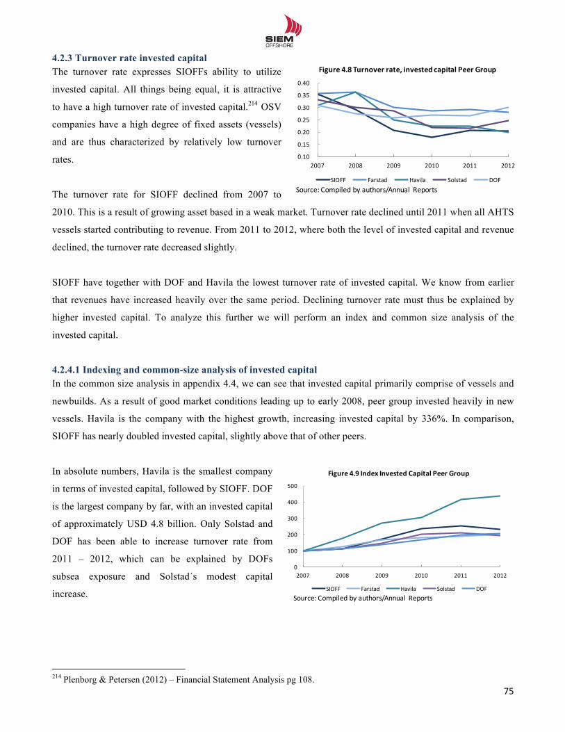
!!
75!!
4.2.3 Turnover rate invested capital The turnover rate expresses SIOFFs ability to utilize
invested capital. All things being equal, it is attractive
to have a high turnover rate of invested capital.214 OSV
companies have a high degree of fixed assets (vessels)
and are thus characterized by relatively low turnover
rates.
The turnover rate for SIOFF declined from 2007 to
2010. This is a result of growing asset based in a weak market. Turnover rate declined until 2011 when all AHTS
vessels started contributing to revenue. From 2011 to 2012, where both the level of invested capital and revenue
declined, the turnover rate decreased slightly.
SIOFF have together with DOF and Havila the lowest turnover rate of invested capital. We know from earlier
that revenues have increased heavily over the same period. Declining turnover rate must thus be explained by
higher invested capital. To analyze this further we will perform an index and common size analysis of the
invested capital.
4.2.4.1 Indexing and common-size analysis of invested capital In the common size analysis in appendix 4.4, we can see that invested capital primarily comprise of vessels and
newbuilds. As a result of good market conditions leading up to early 2008, peer group invested heavily in new
vessels. Havila is the company with the highest growth, increasing invested capital by 336%. In comparison,
SIOFF has nearly doubled invested capital, slightly above that of other peers.
In absolute numbers, Havila is the smallest company
in terms of invested capital, followed by SIOFF. DOF
is the largest company by far, with an invested capital
of approximately USD 4.8 billion. Only Solstad and
DOF has been able to increase turnover rate from
2011 – 2012, which can be explained by DOFs
subsea exposure and Solstad´s modest capital
increase.
!!!!!!!!!!!!!!!!!!!!!!!!!!!!!!!!!!!!!!!!!!!!!!!!!!!!!!!!!!!!!214 Plenborg & Petersen (2012) – Financial Statement Analysis pg 108.
0.10$
0.15$
0.20$
0.25$
0.30$
0.35$
0.40$
2007 2008 2009 2010 2011 2012
Figure'4.8'Turnover'rate,'invested'capital'Peer'Group
SIOFF Farstad Havila Solstad DOFSource:$Compiled by$authors/Annual Reports
0
100
200
300
400
500
2007 2008 2009 2010 2011 2012
Figure'4.9'Index'Invested'Capital'Peer'Group
SIOFF Farstad Havila Solstad DOFSource:=Compiled by=authors/Annual Reports
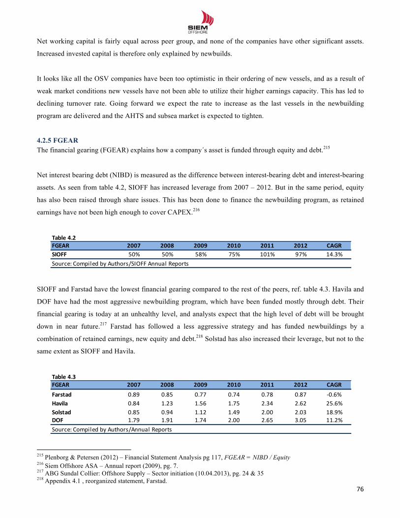
!!
76!!
Net working capital is fairly equal across peer group, and none of the companies have other significant assets.
Increased invested capital is therefore only explained by newbuilds.
It looks like all the OSV companies have been too optimistic in their ordering of new vessels, and as a result of
weak market conditions new vessels have not been able to utilize their higher earnings capacity. This has led to
declining turnover rate. Going forward we expect the rate to increase as the last vessels in the newbuilding
program are delivered and the AHTS and subsea market is expected to tighten.
4.2.5 FGEAR The financial gearing (FGEAR) explains how a company´s asset is funded through equity and debt.215
Net interest bearing debt (NIBD) is measured as the difference between interest-bearing debt and interest-bearing
assets. As seen from table 4.2, SIOFF has increased leverage from 2007 – 2012. But in the same period, equity
has also been raised through share issues. This has been done to finance the newbuilding program, as retained
earnings have not been high enough to cover CAPEX.216
SIOFF and Farstad have the lowest financial gearing compared to the rest of the peers, ref. table 4.3. Havila and
DOF have had the most aggressive newbuilding program, which have been funded mostly through debt. Their
financial gearing is today at an unhealthy level, and analysts expect that the high level of debt will be brought
down in near future.217 Farstad has followed a less aggressive strategy and has funded newbuildings by a
combination of retained earnings, new equity and debt.218 Solstad has also increased their leverage, but not to the
same extent as SIOFF and Havila.
!!!!!!!!!!!!!!!!!!!!!!!!!!!!!!!!!!!!!!!!!!!!!!!!!!!!!!!!!!!!!215 Plenborg & Petersen (2012) – Financial Statement Analysis pg 117, FGEAR = NIBD / Equity 216 Siem Offshore ASA – Annual report (2009), pg. 7. 217 ABG Sundal Collier: Offshore Supply – Sector initiation (10.04.2013), pg. 24 & 35 218 Appendix 4.1 , reorganized statement, Farstad.
FGEAR 2007 2008 2009 2010 2011 2012 CAGRSIOFF 50% 50% 58% 75% 101% 97% 14.3%
Table54.2
Source:2Compiled2by2Authors/SIOFF2Annual2Reports
FGEAR 2007 2008 2009 2010 2011 2012 CAGRFarstad 0.89% 0.85% 0.77% 0.74% 0.78% 0.87% )0.6%Havila 0.84% 1.23% 1.56% 1.75% 2.34% 2.62% 25.6%Solstad 0.85% 0.94% 1.12% 1.49% 2.00% 2.03% 18.9%DOF 1.79% 1.91% 1.74% 2.00% 2.65% 3.05% 11.2%Source:%Compiled%by%Authors/Annual%Reports
Table=4.3
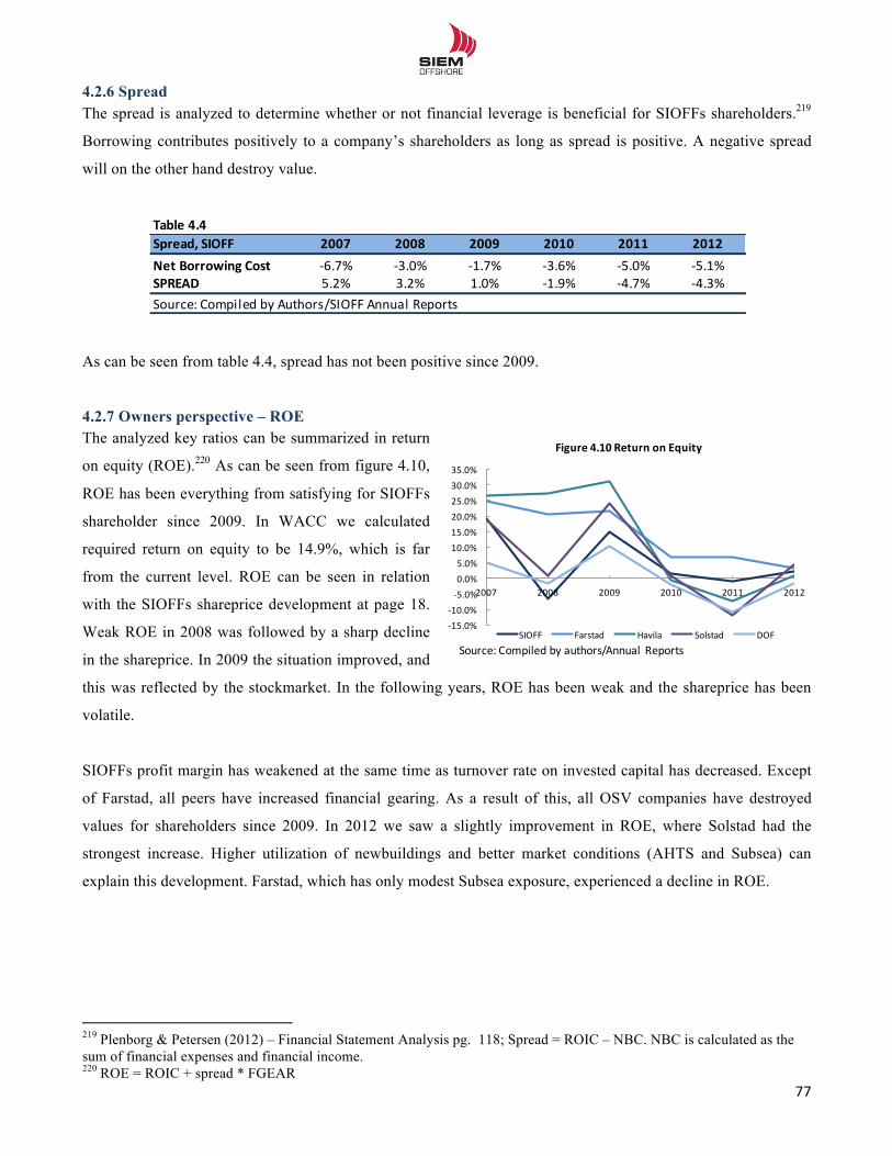
!!
77!!
4.2.6 Spread The spread is analyzed to determine whether or not financial leverage is beneficial for SIOFFs shareholders.219
Borrowing contributes positively to a company’s shareholders as long as spread is positive. A negative spread
will on the other hand destroy value.
As can be seen from table 4.4, spread has not been positive since 2009.
4.2.7 Owners perspective – ROE The analyzed key ratios can be summarized in return
on equity (ROE).220 As can be seen from figure 4.10,
ROE has been everything from satisfying for SIOFFs
shareholder since 2009. In WACC we calculated
required return on equity to be 14.9%, which is far
from the current level. ROE can be seen in relation
with the SIOFFs shareprice development at page 18.
Weak ROE in 2008 was followed by a sharp decline
in the shareprice. In 2009 the situation improved, and
this was reflected by the stockmarket. In the following years, ROE has been weak and the shareprice has been
volatile.
SIOFFs profit margin has weakened at the same time as turnover rate on invested capital has decreased. Except
of Farstad, all peers have increased financial gearing. As a result of this, all OSV companies have destroyed
values for shareholders since 2009. In 2012 we saw a slightly improvement in ROE, where Solstad had the
strongest increase. Higher utilization of newbuildings and better market conditions (AHTS and Subsea) can
explain this development. Farstad, which has only modest Subsea exposure, experienced a decline in ROE.
!!
!!!!!!!!!!!!!!!!!!!!!!!!!!!!!!!!!!!!!!!!!!!!!!!!!!!!!!!!!!!!!219 Plenborg & Petersen (2012) – Financial Statement Analysis pg. 118; Spread = ROIC – NBC. NBC is calculated as the sum of financial expenses and financial income. 220 ROE = ROIC + spread * FGEAR
Spread,(SIOFF 2007 2008 2009 2010 2011 2012Net(Borrowing(Cost !6.7% !3.0% !1.7% !3.6% !5.0% !5.1%SPREAD 5.2% 3.2% 1.0% !1.9% !4.7% !4.3%
Table(4.4
Source:4Compiled4by4Authors/SIOFF4Annual4Reports
!15.0%!10.0%!5.0%0.0%5.0%
10.0%15.0%20.0%25.0%30.0%35.0%
2007 2008 2009 2010 2011 2012
Figure'4.10'Return'on'Equity
SIOFF Farstad Havila Solstad DOFSource:?Compiled by?authors/Annual Reports
!!
78!!
4.3 Liquidity Risk Analysis 4.3.1 Short-term liquidity risk Liquidity is a crucial subject for any business, as lack of liquidity might be a barrier to exploit profitable business
opportunities. A firm’s liquidity risk is influenced by its ability to generate positive net cash flows in both short
and long term.221 The short term analysis will uncover SIOFFs ability to meet all short-term obligations as they
fall due. The long-term liquidity risk/solvency risk will measure SIOFFs long-term financial health and ability to
cover long-term obligations. All liquidity ratios are based on ending year balances, as these are considered the
most updated.222 These ratios will be used as input to determine SIOFFs WACC in part 7.0.
Liquidity cycle
An indicator of the short-term liquidity risk is the number of days it takes to convert working capital to cash.223
The fewer days it takes, the better the cash flow. The liquidity cycle can be seen in table 4.5.
SIOFFs liquidity cycle has improved in recent years, which is a result of increased revenue and tight
management of working capital. Even while revenue has increased strongly, SIOFF has managed to maintain
working capital at almost the same level, as can be seen in common size analysis. Compared to peers SIOFFs
ratio is slightly higher, indicating a higher working capital and higher liquidity risk. However we do not believe
that the ratio indicates liquidity problems, as it has improved steadily since 2007. In comparison, we believe
there is a greater potential for liquidity problems for Havila, as current liabilities exceeds current assets.
!!!!!!!!!!!!!!!!!!!!!!!!!!!!!!!!!!!!!!!!!!!!!!!!!!!!!!!!!!!!!221 Plenborg & Petersen (2012) – Financial Statement Analysis pg. 150 222 Plenborg & Petersen (2012) – Financial Statement Analysis pg. 155 223 Plenborg & Petersen (2012) – Financial Statement Analysis pg. 153, liquidity cycle = 365 / (revenue / net working capital))
Table&4.5Liquidity&cycle 2007 2008 2009 2010 2011 2012SIOFF 63.4 35.5 36.8 41.4 35.3 29.9Farstad 25.2 33.6 41.3 8.7 7.7 20.7Havila (180.2) (84.0) (37.5) (117.0) (42.9) (155.2)Solstad 63.5 32.1 37.5 11.0 30.4 10.2DOF 41.4 36.5 89.2 43.3 28.1 30.9Average 48.4 34.4 51.2 26.1 25.4 22.9Source:5Compiled5by5Authors/Annual5Reports
!!
79!!
Current ratio
The current ratio is an alternative measure for the short term liquidity. The basic idea is to see how much of the
current assets that cover current liabilities in the event of liquidation.224
Some argue that a ratio above 2 is an indication of low liquidity risk, but this is difficult to generalize across
different industries.225 Therefore we have benchmarked SIOFFs ratio towards the peer-group. As can be seen
from table 4.6, SIOFF has a ratio above average. The ratio has also been very stable, and there is no signal of
liquidity problems.
4.3.2 Long term liquidity risk Solvency ratio
One indicator of long-term liquidity risk is the solvency ratio.226 We have calculated the ratios based on market
values, as these are closer to realizable values. The historical development can be seen in table 4.7, and the
calculation can be seen in appendix 4.5.
Over the last three years SIOFF had the second highest solvency ratio, only exceed by Farstad. The ratio has
declined since 2007, as a result of poor share price performance. However, SIOFF have a higher ratio compared
to peers, which gives them freedom to make new fleet investments.
!!!!!!!!!!!!!!!!!!!!!!!!!!!!!!!!!!!!!!!!!!!!!!!!!!!!!!!!!!!!!224 Plenborg & Petersen (2012) – Financial Statement Analysis pg. 155, Current ratio = current assets / current liabilities 225 Plenborg & Petersen (2012) – Financial Statement Analysis pg. 156. 226 Plenborg & Petersen (2012) – Financial Statement Analysis pg. 158, Solvency ratio = Equity / (NIBD + Equity)
Table&4.6Current&ratio 2007 2008 2009 2010 2011 2012SIOFF 2.6 1.6 1.5 1.3 1.5 1.6Farstad 1.4 1.5 1.6 1.9 1.1 1.1Havila 1.6 0.3 0.6 0.8 0.6 0.7Solstad 1.9 2.0 1.4 1.5 1.1 1.4DOF 1.3 1.6 1.4 2.7 1.5 1.3Average 1.8 1.4 1.3 1.6 1.2 1.2Source:3Compiled3by3Authors/Annual3Reports
Table&4.7Solvency&ratio,&market&values 2007 2008 2009 2010 2011 2012SIOFF 84% 56% 59% 51% 40% 44%Farstad 65% 42% 52% 58% 52% 45%Havila 72% 24% 26% 23% 13% 12%Solstad 65% 37% 42% 33% 25% 31%DOF 36% 22% 23% 22% 11% 13%Average 64% 36% 41% 37% 28% 29%Source:3Compiled3by3Authors/Annual3Reports
!!
80!!
Interest coverage ratio
The interest coverage ratio measures SIOFFs ability to meet its net financial expenses. The ratio shows how
many times operating profit covers net financial expenses.227 However, there are very different rules of thumbs in
different industries, thus we need to compare the ratio with the peer group.
When looking at EBITDA Interest coverage ratio we exclude the effect of depreciation, as this does not represent
an actual cash flow. As seen from table 4.8, SIOFF has been well above average, for the whole period. From
2009 and until today, there has been a declining ratio, indicating an increase in the long-term liquidity risk. This
is applicable for all the peers.
A more conservative measure is the EBIT-interest coverage ratio. By using this measure we include
depreciations, which is an expression of the investment needed to maintain the size of the asset base.
In table 4.9 we can see that SIOFFs ratio is below average in 2011 and 2012, indicating higher long term
liquidity risk compared to peers. If the ratio stays below one it can affect SIOFFs ability to meet long term
financial obligations.
!!!!!!!!!!!!!!!!!!!!!!!!!!!!!!!!!!!!!!!!!!!!!!!!!!!!!!!!!!!!!227 Plenborg & Petersen (2012) – Financial Statement Analysis pg. 161; Interest coverage ratio = EBIT / Net financial expenses
Table&4.8EBITDA&interest&coverage&ratio 2007 2008 2009 2010 2011 2012SIOFF 7.3 8.0 12.1 11.0 4.2 2.9Farstad 5.8 6.6 7.5 7.7 4.3 4.0Havila 7.8 3.8 1.7 (9.8) 1.2 1.2Solstad (5.3) (14.9) 1.8 (7.4) 4.1 2.1DOF 6.6 3.0 2.0 4.4 2.1 1.8Average 4.4 1.3 5.0 1.2 3.2 2.4Source:5Compiled5by5Authors/Annual5Reports
Table&4.9EBIT&interest&coverage&ratio 2007 2008 2009 2010 2011 2012SIOFF 5.0 6.2 7.3 4.2 1.2 0.8Farstad 4.1 4.7 5.9 5.7 2.7 2.5Havila 6.1 2.9 1.3 (6.9) 0.5 0.6Solstad (3.5) (9.8) 1.0 (2.9) 1.4 0.3DOF 4.3 1.7 1.0 1.3 0.7 1.0Average 3.2 1.1 3.3 0.3 1.3 1.1Source:5Compiled5by5Authors/Annual5Reports
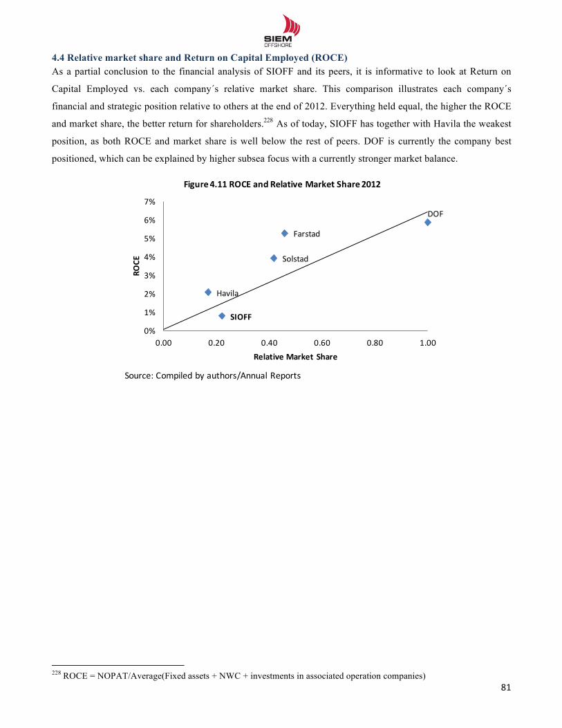
!!
81!!
4.4 Relative market share and Return on Capital Employed (ROCE) As a partial conclusion to the financial analysis of SIOFF and its peers, it is informative to look at Return on
Capital Employed vs. each company´s relative market share. This comparison illustrates each company´s
financial and strategic position relative to others at the end of 2012. Everything held equal, the higher the ROCE
and market share, the better return for shareholders.228 As of today, SIOFF has together with Havila the weakest
position, as both ROCE and market share is well below the rest of peers. DOF is currently the company best
positioned, which can be explained by higher subsea focus with a currently stronger market balance.!
!!!!!!!!!!!!!!!!!!!!!!!!!!!!!!!!!!!!!!!!!!!!!!!!!!!!!!!!!!!!!228 ROCE = NOPAT/Average(Fixed assets + NWC + investments in associated operation companies)
SIOFF
Farstad
Havila
Solstad
DOF
0%
1%
2%
3%
4%
5%
6%
7%
0.00 0.20 0.40 0.60 0.80 1.00
ROCE
Relative.Market.Share
Figure.4.11.ROCE.and.Relative.Market.Share.2012
Source:>Compiled by>authors/Annual Reports
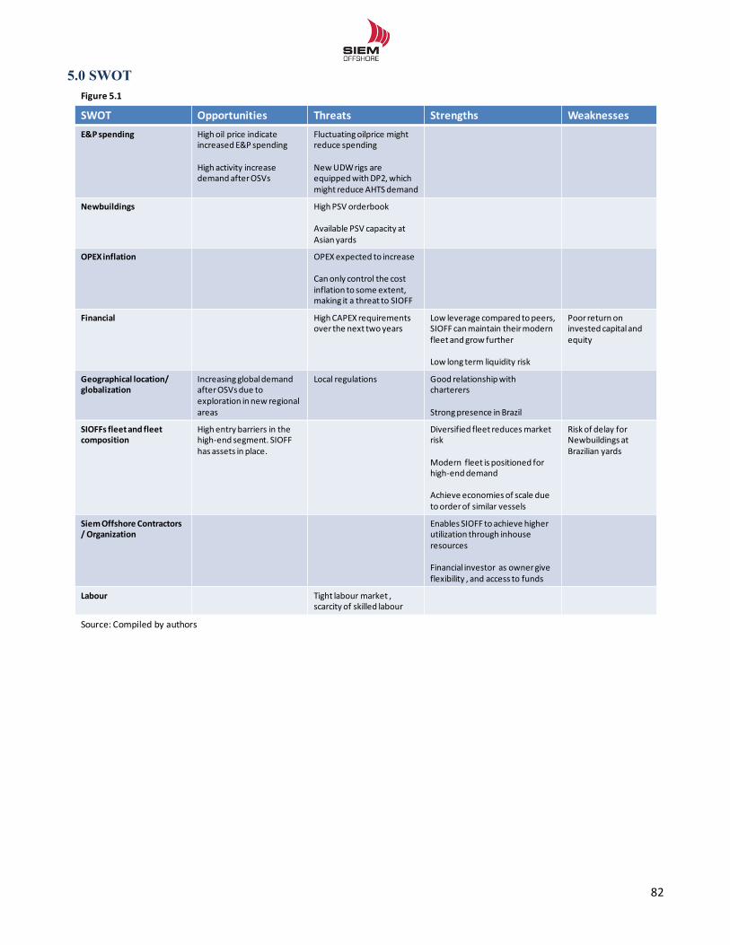
!!
82!!
5.0 SWOT
SWOT Opportunities Threats Strengths WeaknessesE&P5spending High%oil%price%indicate
increased%E&P%spending
High%activity%increase%demand%after%OSVs
Fluctuatingoilprice might%reduce%spending
New%UDW%rigs%areequippedwithDP2,%which%might%reduce%AHTS%demand
Newbuildings High%PSV orderbook
Available PSV%capacity at%Asian yards
OPEX5inflation OPEX%expected to%increase
Can%only control%the%cost%inflation%to%some%extent,%making%it%a%threat%to%SIOFF
Financial High%CAPEX%requirements%over%the%next%two%years
Low%leverage%compared%to%peers,%SIOFF%can%maintain%their%modern%fleet%and%grow%further
Low%long%term%liquidity%risk
Poor%return on%invested%capital%and%equity
Geographical5location/5globalization
Increasing%global%demand%after%OSVs%due%to%exploration%in%new%regional%areas
Local regulations Good%relationship%with%charterers
Strong%presence%in%Brazil
SIOFFs5fleet5and5fleet5composition
Highentry barriers in%the%highQend segment. SIOFF%has%assets%in%place.
Diversified%fleet%reducesmarket%risk
Modern%%fleet%is%positioned%for%highQend%demand
Achieve%economies%of%scale%due%to%order%of%similar%vessels
Risk%of delay%for%Newbuildings%at%Brazilian%yards
SiemOffshore5Contractors5/5Organization
Enables SIOFF%to%achieve%higher%utilization%through%inhouseresources
Financial%investor%%as%owner%give%flexibility%,%and%access%to%funds
Labour Tight labour market ,%scarcity of%skilled labour
Figure 5.1
Source:%Compiled by%authors
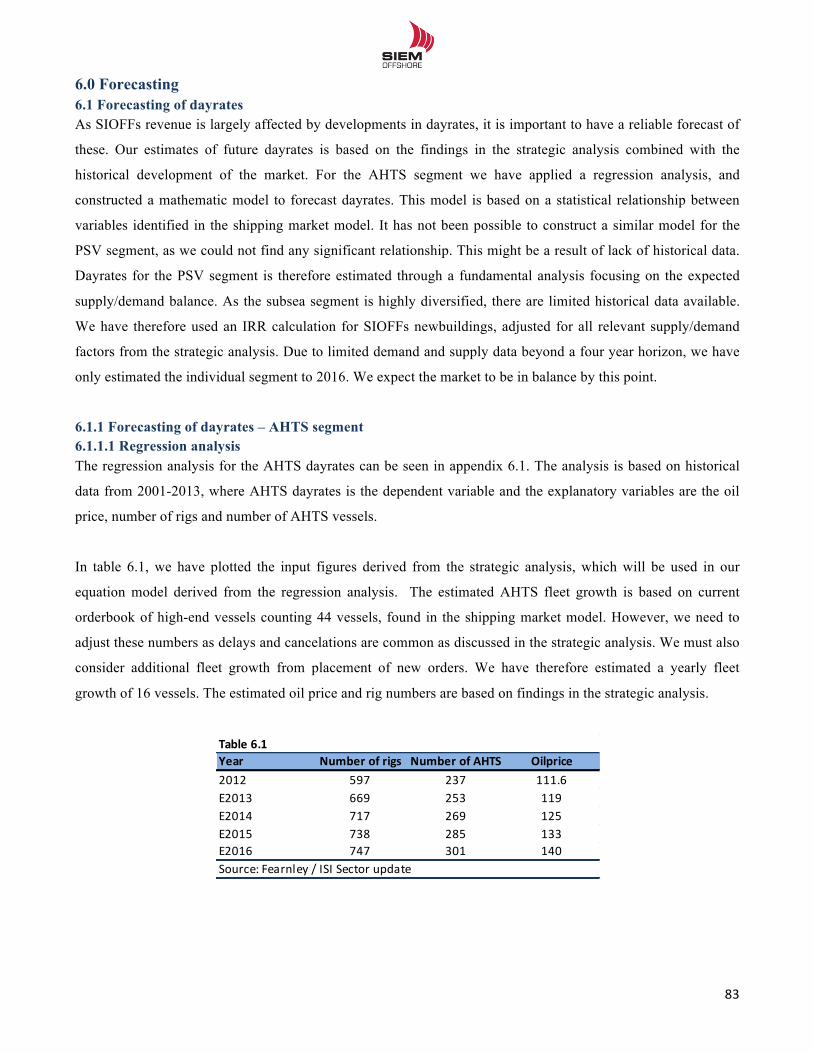
!!
83!!
6.0 Forecasting 6.1 Forecasting of dayrates As SIOFFs revenue is largely affected by developments in dayrates, it is important to have a reliable forecast of
these. Our estimates of future dayrates is based on the findings in the strategic analysis combined with the
historical development of the market. For the AHTS segment we have applied a regression analysis, and
constructed a mathematic model to forecast dayrates. This model is based on a statistical relationship between
variables identified in the shipping market model. It has not been possible to construct a similar model for the
PSV segment, as we could not find any significant relationship. This might be a result of lack of historical data.
Dayrates for the PSV segment is therefore estimated through a fundamental analysis focusing on the expected
supply/demand balance. As the subsea segment is highly diversified, there are limited historical data available.
We have therefore used an IRR calculation for SIOFFs newbuildings, adjusted for all relevant supply/demand
factors from the strategic analysis. Due to limited demand and supply data beyond a four year horizon, we have
only estimated the individual segment to 2016. We expect the market to be in balance by this point.
6.1.1 Forecasting of dayrates – AHTS segment 6.1.1.1 Regression analysis The regression analysis for the AHTS dayrates can be seen in appendix 6.1. The analysis is based on historical
data from 2001-2013, where AHTS dayrates is the dependent variable and the explanatory variables are the oil
price, number of rigs and number of AHTS vessels.
In table 6.1, we have plotted the input figures derived from the strategic analysis, which will be used in our
equation model derived from the regression analysis. The estimated AHTS fleet growth is based on current
orderbook of high-end vessels counting 44 vessels, found in the shipping market model. However, we need to
adjust these numbers as delays and cancelations are common as discussed in the strategic analysis. We must also
consider additional fleet growth from placement of new orders. We have therefore estimated a yearly fleet
growth of 16 vessels. The estimated oil price and rig numbers are based on findings in the strategic analysis.
Table&6.1Year Number&of&rigs Number&of&AHTS Oilprice2012 597 237 111.6E2013 669 253 119E2014 717 269 125E2015 738 285 133E2016 747 301 140Source:4Fearnley4/4ISI4Sector4update4
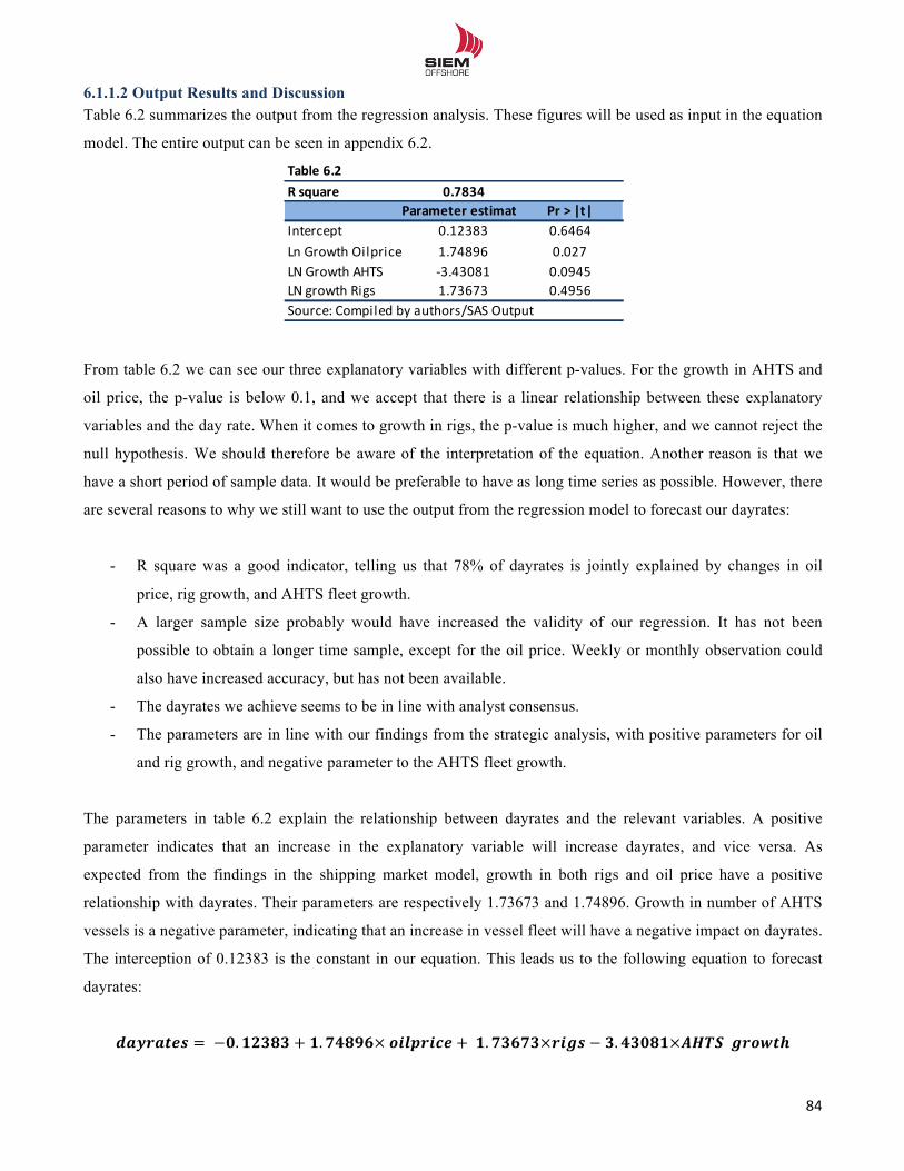
!!
84!!
6.1.1.2 Output Results and Discussion Table 6.2 summarizes the output from the regression analysis. These figures will be used as input in the equation
model. The entire output can be seen in appendix 6.2.
From table 6.2 we can see our three explanatory variables with different p-values. For the growth in AHTS and
oil price, the p-value is below 0.1, and we accept that there is a linear relationship between these explanatory
variables and the day rate. When it comes to growth in rigs, the p-value is much higher, and we cannot reject the
null hypothesis. We should therefore be aware of the interpretation of the equation. Another reason is that we
have a short period of sample data. It would be preferable to have as long time series as possible. However, there
are several reasons to why we still want to use the output from the regression model to forecast our dayrates:
- R square was a good indicator, telling us that 78% of dayrates is jointly explained by changes in oil
price, rig growth, and AHTS fleet growth.
- A larger sample size probably would have increased the validity of our regression. It has not been
possible to obtain a longer time sample, except for the oil price. Weekly or monthly observation could
also have increased accuracy, but has not been available.
- The dayrates we achieve seems to be in line with analyst consensus.
- The parameters are in line with our findings from the strategic analysis, with positive parameters for oil
and rig growth, and negative parameter to the AHTS fleet growth.
The parameters in table 6.2 explain the relationship between dayrates and the relevant variables. A positive
parameter indicates that an increase in the explanatory variable will increase dayrates, and vice versa. As
expected from the findings in the shipping market model, growth in both rigs and oil price have a positive
relationship with dayrates. Their parameters are respectively 1.73673 and 1.74896. Growth in number of AHTS
vessels is a negative parameter, indicating that an increase in vessel fleet will have a negative impact on dayrates.
The interception of 0.12383 is the constant in our equation. This leads us to the following equation to forecast
dayrates:
!"#$"%&' = !−!.!"#$# + !.!"#$%×!!"#$%"&' + !!.!"#!"×!"#$ − !.!"#$%×!"#$!!!"#$%&
Table&6.2R&square 0.7834
Parameter&estimate Pr&>&|t|Intercept 0.12383 0.6464Ln1Growth1Oilprice 1.74896 0.027LN1Growth1AHTS @3.43081 0.0945LN1growth1Rigs 1.73673 0.4956Source:1Compiled1by1authors/SAS1Output
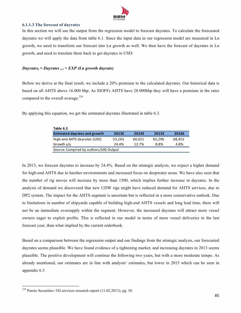
!!
85!!
6.1.1.3 The forecast of dayrates In this section we will use the output from the regression model to forecast dayrates. To calculate the forecasted
dayrates we will apply the data from table 6.1. Since the input data in our regression model are measured in Ln
growth, we need to transform our forecast into Ln growth as well. We then have the forecast of dayrates in Ln
growth, and need to translate them back to get dayrates in USD:
Dayratest = Dayrates t-1 × EXP (Ln growth dayrate)
Before we derive at the final result, we include a 20% premium to the calculated dayrates. Our historical data is
based on all AHTS above 16.000 bhp. As SIOFFs AHTS have 28.000bhp they will have a premium in the rates
compared to the overall average.229
By applying this equation, we get the estimated dayrates illustrated in table 6.3.
In 2013, we forecast dayrates to increase by 24.4%. Based on the strategic analysis, we expect a higher demand
for high-end AHTS due to harsher environments and increased focus on deepwater areas. We have also seen that
the number of rig moves will increase by more than 1500, which implies further increase in dayrates. In the
analysis of demand we discovered that new UDW rigs might have reduced demand for AHTS services, due to
DP2 system. The impact for the AHTS segment is uncertain but is reflected in a more conservative outlook. Due
to limitations in number of shipyards capable of building high-end AHTS vessels and long lead time, there will
not be an immediate oversupply within the segment. However, the increased dayrates will attract more vessel
owners eager to exploit profits. This is reflected in our model in terms of more vessel deliveries in the last
forecast year, than what implied by the current orderbook.
Based on a comparison between the regression output and our findings from the strategic analysis, our forecasted
dayrates seems plausible. We have found evidence of a tightening market, and increasing dayrates in 2013 seems
plausible. The positive development will continue the following two years, but with a more moderate tempo. As
already mentioned, our estimates are in line with analysts’ estimates, but lower in 2015 which can be seen in
appendix 6.3
!!!!!!!!!!!!!!!!!!!!!!!!!!!!!!!!!!!!!!!!!!!!!!!!!!!!!!!!!!!!!229 Pareto Securities: Oil services research report (11.02.2013), pg. 56
Table&6.3Estimated&dayrates&and&growth 2013E 2014E 2015E 2016EHigh%end)AHTS)dayrates)(USD) 53,243 60,021 65,296 68,452Growth)y/y 24.4% 12.7% 8.8% 4.8%Source:)Compiled)by)authors/SAS)Output
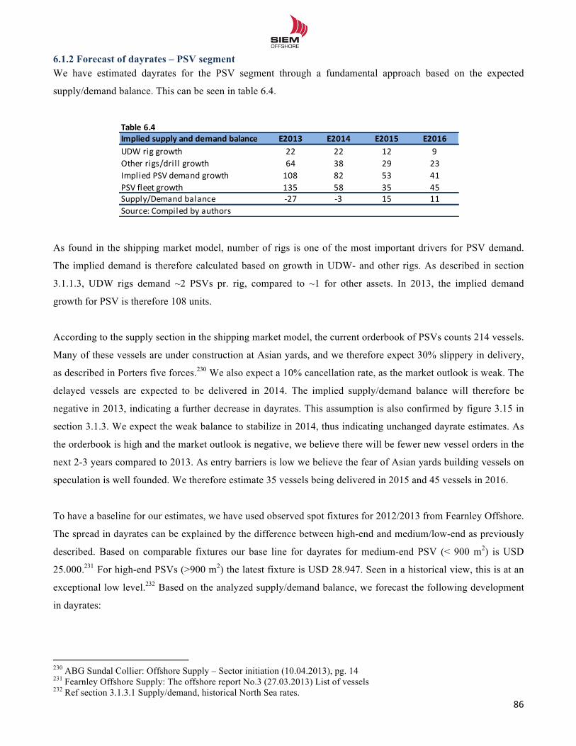
!!
86!!
6.1.2 Forecast of dayrates – PSV segment We have estimated dayrates for the PSV segment through a fundamental approach based on the expected
supply/demand balance. This can be seen in table 6.4.
As found in the shipping market model, number of rigs is one of the most important drivers for PSV demand.
The implied demand is therefore calculated based on growth in UDW- and other rigs. As described in section
3.1.1.3, UDW rigs demand ~2 PSVs pr. rig, compared to ~1 for other assets. In 2013, the implied demand
growth for PSV is therefore 108 units.
According to the supply section in the shipping market model, the current orderbook of PSVs counts 214 vessels.
Many of these vessels are under construction at Asian yards, and we therefore expect 30% slippery in delivery,
as described in Porters five forces.230 We also expect a 10% cancellation rate, as the market outlook is weak. The
delayed vessels are expected to be delivered in 2014. The implied supply/demand balance will therefore be
negative in 2013, indicating a further decrease in dayrates. This assumption is also confirmed by figure 3.15 in
section 3.1.3. We expect the weak balance to stabilize in 2014, thus indicating unchanged dayrate estimates. As
the orderbook is high and the market outlook is negative, we believe there will be fewer new vessel orders in the
next 2-3 years compared to 2013. As entry barriers is low we believe the fear of Asian yards building vessels on
speculation is well founded. We therefore estimate 35 vessels being delivered in 2015 and 45 vessels in 2016.
To have a baseline for our estimates, we have used observed spot fixtures for 2012/2013 from Fearnley Offshore.
The spread in dayrates can be explained by the difference between high-end and medium/low-end as previously
described. Based on comparable fixtures our base line for dayrates for medium-end PSV (< 900 m2) is USD
25.000.231 For high-end PSVs (>900 m2) the latest fixture is USD 28.947. Seen in a historical view, this is at an
exceptional low level.232 Based on the analyzed supply/demand balance, we forecast the following development
in dayrates:
!!!!!!!!!!!!!!!!!!!!!!!!!!!!!!!!!!!!!!!!!!!!!!!!!!!!!!!!!!!!!230 ABG Sundal Collier: Offshore Supply – Sector initiation (10.04.2013), pg. 14 231 Fearnley Offshore Supply: The offshore report No.3 (27.03.2013) List of vessels 232 Ref section 3.1.3.1 Supply/demand, historical North Sea rates.
Table&6.4Implied&supply&and&demand&balance& E2013 E2014 E2015 E2016UDW$rig$growth 22 22 12 9
Other$rigs/drill $growth 64 38 29 23
Implied$PSV$demand$growth 108 82 53 41
PSV$fleet$growth 135 58 35 45
Supply/Demand$balance H27 H3 15 11
Source:$Compiled$by$authors
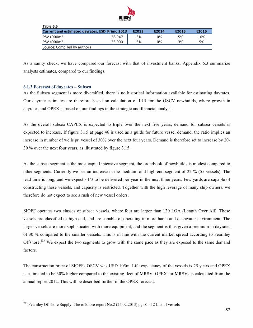
!!
87!!
As a sanity check, we have compared our forecast with that of investment banks. Appendix 6.3 summarize
analysts estimates, compared to our findings.
6.1.3 Forecast of dayrates – Subsea As the Subsea segment is more diversified, there is no historical information available for estimating dayrates.
Our dayrate estimates are therefore based on calculation of IRR for the OSCV newbuilds, where growth in
dayrates and OPEX is based on our findings in the strategic and financial analysis.
As the overall subsea CAPEX is expected to triple over the next five years, demand for subsea vessels is
expected to increase. If figure 3.15 at page 46 is used as a guide for future vessel demand, the ratio implies an
increase in number of wells pr. vessel of 30% over the next four years. Demand is therefore set to increase by 20-
30 % over the next four years, as illustrated by figure 3.15.
As the subsea segment is the most capital intensive segment, the orderbook of newbuilds is modest compared to
other segments. Currently we see an increase in the medium- and high-end segment of 22 % (55 vessels). The
lead time is long, and we expect ~1/3 to be delivered per year in the next three years. Few yards are capable of
constructing these vessels, and capacity is restricted. Together with the high leverage of many ship owners, we
therefore do not expect to see a rush of new vessel orders.
SIOFF operates two classes of subsea vessels, where four are larger than 120 LOA (Length Over All). These
vessels are classified as high-end, and are capable of operating in more harsh and deepwater environment. The
larger vessels are more sophisticated with more equipment, and the segment is thus given a premium in dayrates
of 30 % compared to the smaller vessels. This is in line with the current market spread according to Fearnley
Offshore.233 We expect the two segments to grow with the same pace as they are exposed to the same demand
factors.
The construction price of SIOFFs OSCV was USD 105m. Life expectancy of the vessels is 25 years and OPEX
is estimated to be 30% higher compared to the existing fleet of MRSV. OPEX for MRSVs is calculated from the
annual report 2012. This will be described further in the OPEX forecast.
!!!!!!!!!!!!!!!!!!!!!!!!!!!!!!!!!!!!!!!!!!!!!!!!!!!!!!!!!!!!!233 Fearnley Offshore Supply: The offshore report No.2 (25.02.2013) pg. 8 – 12 List of vessels
Table&6.5Current&and&estimated&dayrates,&USD Primo&2013 E2013 E2014 E2015 E2016PSV$>900m2 28,947 .3% 0% 5% 10%PSV$<900m2 25,000 .5% 0% 3% 5%Source:$Compiled$by$authors
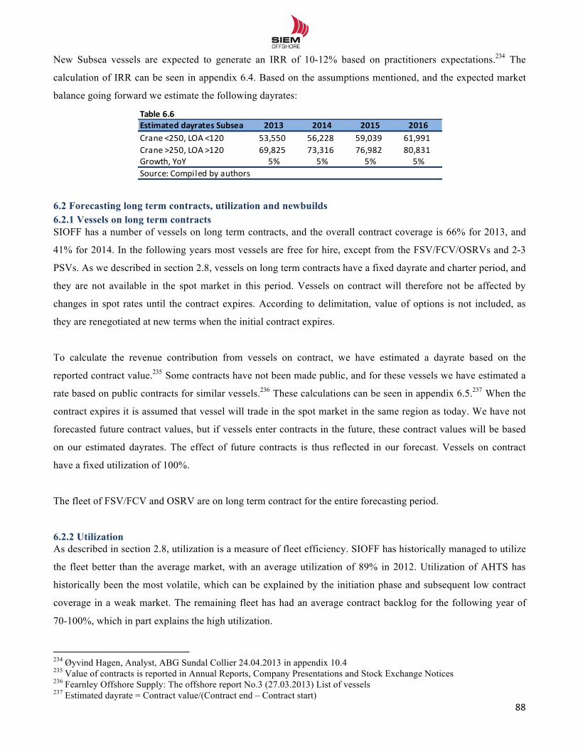
!!
88!!
New Subsea vessels are expected to generate an IRR of 10-12% based on practitioners expectations.234 The
calculation of IRR can be seen in appendix 6.4. Based on the assumptions mentioned, and the expected market
balance going forward we estimate the following dayrates:
6.2 Forecasting long term contracts, utilization and newbuilds 6.2.1 Vessels on long term contracts SIOFF has a number of vessels on long term contracts, and the overall contract coverage is 66% for 2013, and
41% for 2014. In the following years most vessels are free for hire, except from the FSV/FCV/OSRVs and 2-3
PSVs. As we described in section 2.8, vessels on long term contracts have a fixed dayrate and charter period, and
they are not available in the spot market in this period. Vessels on contract will therefore not be affected by
changes in spot rates until the contract expires. According to delimitation, value of options is not included, as
they are renegotiated at new terms when the initial contract expires.
To calculate the revenue contribution from vessels on contract, we have estimated a dayrate based on the
reported contract value.235 Some contracts have not been made public, and for these vessels we have estimated a
rate based on public contracts for similar vessels.236 These calculations can be seen in appendix 6.5.237 When the
contract expires it is assumed that vessel will trade in the spot market in the same region as today. We have not
forecasted future contract values, but if vessels enter contracts in the future, these contract values will be based
on our estimated dayrates. The effect of future contracts is thus reflected in our forecast. Vessels on contract
have a fixed utilization of 100%.
The fleet of FSV/FCV and OSRV are on long term contract for the entire forecasting period.
6.2.2 Utilization As described in section 2.8, utilization is a measure of fleet efficiency. SIOFF has historically managed to utilize
the fleet better than the average market, with an average utilization of 89% in 2012. Utilization of AHTS has
historically been the most volatile, which can be explained by the initiation phase and subsequent low contract
coverage in a weak market. The remaining fleet has had an average contract backlog for the following year of
70-100%, which in part explains the high utilization.
!!!!!!!!!!!!!!!!!!!!!!!!!!!!!!!!!!!!!!!!!!!!!!!!!!!!!!!!!!!!!234 Øyvind Hagen, Analyst, ABG Sundal Collier 24.04.2013 in appendix 10.4 235 Value of contracts is reported in Annual Reports, Company Presentations and Stock Exchange Notices 236 Fearnley Offshore Supply: The offshore report No.3 (27.03.2013) List of vessels 237 Estimated dayrate = Contract value/(Contract end – Contract start)
Table&6.6Estimated&dayrates&Subsea 2013 2014 2015 2016Crane&<250,&LOA&<120 53,550 56,228 59,039 61,991Crane&>250,&LOA&>120 69,825 73,316 76,982 80,831Growth,&YoY 5% 5% 5% 5%Source:&Compiled&by&authors
!!
89!!
SIOFFs ability to obtain above average utilization can be explained by our findings in the internal analysis. The
management has a good track record when it comes to optimization of fleet composition and geographical
location. By managing the fleet in this way, SIOFF has taken advantage of new growth areas such as Brazil and
West Africa. Through the Brazilian subsidiary, SIOFF has been able to create relations with the region´s most
important petroleum client. In the Porter analysis we concluded that bargaining power for buyers to be moderate.
SIOFFs good reputation and collaboration with buyers has therefore secured contracts and vessel employment. In
addition, SIOFFs strategy of increased exposure towards high-end vessels has made SIOFF able to earn a
utilization premium compared to low-end tonnage. We believe SIOFF have an attractive fleet of modern vessels
and a management team capable of meeting new demand trends. The combined resources represent a competitive
advantage which is supportive for a utilization premium going forward.
SIOFFs forecast of utilization is positively affected by the subsidiary Siem Offshore Contractors. As previously
described, SOC has a contract backlog of approximately USD 180m over the next 24 months. To execute these
contracts, SOC utilize in-house resources in terms of vessels and equipment. SIOFF can therefore utilize
unemployed vessels to their in-house operations. We therefore expect the fleet to obtain an additional utilization
premium compared to the general market. The value of SOC is therefore reflected through this higher utilization.
Due to the nature of the work, we expect a utilization premium of 3 % for the subsea fleet and 2 % for the high-
end AHTS and PSV fleet.
Utilization for SIOFFs PSVs has fluctuated between 91 and 96% the last four years, despite weak market
conditions. This is significantly higher than the average market utilization, as we saw in the Shipping Market
Model. The market is expected to remain oversupplied in the next two years, as the entry barriers are low and
Asian yards are building on speculation. We are therefore somewhat conservative in our estimate for utilization
in 2013. We believe the high-end fleet will be able to obtain a utilization in line with historical average, of 95 %
from 2014 and onwards. We see the utilization spread between high- and low-end widen in the future, as demand
for sophisticated vessels for deepwater/harsh environment will continue. We therefore forecast a utilization of
85% for the medium-end segment, which is below SIOFFs historical average.
For the AHTS segment we expect that a tighter market will increase overall utilization. As the case for PSV, we
expect high-end tonnage to earn a utilization premium. Demand for SIOFFs vessels will therefore be strong. We
expect utilization to increase to 85% in the first year of forecasting, and then increase to 92% in the following
period, including the premium from SOC.
The subsea segment has had a historical utilization close to 100%, and we expect this ratio to remain steady
going forward. With the utilization premium from SOC, the utilization is forecasted to 98% for the entire
forecasting period.
!!
90!!
6.2.3 Newbuildings and demolition The current newbuilding program counts ten vessels with delivery in 2013 and 2014. This will increase SIOFFs
revenue potential significantly and is an important driver of revenue growth. In the forecasting, revenues are
calculated based on the time of delivery of these vessels, as can be seen in appendix 6.6. Four of the vessels are
under construction at Brazilian yards, as part of management’s strategy of increased Brazilian presence. Two
PSVs have estimated delivery Q2 2013 and Q1 2014, and two OSRVs in Q2 2013. As discovered in the Porters
analysis almost all deliveries from these yards are delayed. We therefore estimate these vessels to be delayed by
one quarter, which is reflected in our revenue forecast. Delay of vessels can be seen as a direct cost of
management´s strategy, analyzed in VRIO.
The four OSCV, the ISV and one PSV are built at Norwegian yards. As discovered in the Porters analysis, these
yards are known for high quality and delivery on time. We therefore expect these vessels to be delivered
according to schedule.
After the newbuilding program is concluded, we still expect SIOFF to grow by ordering new vessels. Because of
growth barriers such as financial resources, operational management and yard capacity, we do not expect the
future growth to be as aggressive as we have seen the last 6 years. We therefore expect the fleet to grow by net
one vessel pr. year from 2015. There is no guiding from management indicating witch type of vessels they will
order in the future. Forecast of newbuildings is therefore based on average dayrates across high-end PSV, AHTS
and Subsea, which is our best estimate.
Scrapping has historically been insignificant. But as five of the small Brazilian vessels are above 30-35 years old,
we expect these to be scrapped when the contract expires, in Q2 2014. Two Brazilian OSRVs are also more than
35 years old, and currently unemployed. We therefore expect these vessels to be scrapped Q1 2013.
!!
91!!
6.3 Forecasting of future revenues, expenses and cash flow 6.3.1 Forecast period To estimate the future cash flow of SIOFF through a two-stage DCF and EVA model, we need to choose an
appropriate budget period. As the present value approaches assumes a constant growth rate in the terminal
period, the forecast period must be long enough for the company to reach steady state growth.238 To ensure this
relationship, we must consider management expectations and projected fleet growth.
The forecast period must thus reflect SIOFFs newbuilding program, which will have significant impact on
revenues going forward. Currently many vessels are employed on long term contracts, and this effect must also
be considered. Finally, the forecast period must be long enough to reflect a state of constant supply/demand
balance in the OSV market. Based on these arguments we have chosen a forecast period of 6 years, as we believe
SIOFF to have reached steady state growth by 2018. The OSV industry is a cyclical market with large deviation
from peak to trough. Based on our findings in the strategic and financial analysis we believe the market to be in
balance by 2016, and our estimated dayrates in the last forecast year is in line with the historical average. By
2018 all vessels have finished their long term contracts.
6.3.2 Terminal growth Growth in terminal period shall reflect the expected average growth rate of the economy where the company
operates. SIOFF has operations in different geographical areas and are thus subject to different inflation and
growth rates. As the company is located in Norway and the shareprice is quoted in NOK, we base our estimate
on the growth prospect for the Norwegian economy. According to Norges Bank and the average expectation of
industry professionals, the expected long term nominal earnings growth is 2.5%.239 We see this as a reasonable
growth estimate for the economy and the OSV industry, and it is thus applicable for SIOFF.
6.3.3 Pro forma income statement In the following section we forecast the items in the income statement. The forecast model is based on a sales-
driven approach, with the exception of specified items. This will ensure higher forecast quality, as it provides a
better link between the level of activity and related expenses.240 This reflects that the items forecasted are based
on the expected level of SIOFFs activity. The historical period is used as a guideline in our forecasts as it
provides valuable insights about trends and levels of value drivers. The complete historical development can be
seen in appendix 6.7.
!!!!!!!!!!!!!!!!!!!!!!!!!!!!!!!!!!!!!!!!!!!!!!!!!!!!!!!!!!!!!238 Plenborg & Petersen (2012) – Financial Statement Analysis pg. 214 239 www.norges-bank.no/inflasjon, PwC (2012): “The Norwegian market risk premium 2012-2013” pg. 16 240 Plenborg & Petersen (2012) – Financial Statement Analysis pg. 177
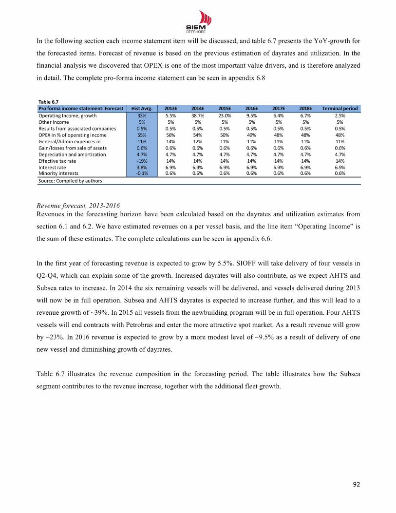
!!
92!!
In the following section each income statement item will be discussed, and table 6.7 presents the YoY-growth for
the forecasted items. Forecast of revenue is based on the previous estimation of dayrates and utilization. In the
financial analysis we discovered that OPEX is one of the most important value drivers, and is therefore analyzed
in detail. The complete pro-forma income statement can be seen in appendix 6.8
Revenue forecast, 2013-2016 Revenues in the forecasting horizon have been calculated based on the dayrates and utilization estimates from
section 6.1 and 6.2. We have estimated revenues on a per vessel basis, and the line item “Operating Income” is
the sum of these estimates. The complete calculations can be seen in appendix 6.6.
In the first year of forecasting revenue is expected to grow by 5.5%. SIOFF will take delivery of four vessels in
Q2-Q4, which can explain some of the growth. Increased dayrates will also contribute, as we expect AHTS and
Subsea rates to increase. In 2014 the six remaining vessels will be delivered, and vessels delivered during 2013
will now be in full operation. Subsea and AHTS dayrates is expected to increase further, and this will lead to a
revenue growth of ~39%. In 2015 all vessels from the newbuilding program will be in full operation. Four AHTS
vessels will end contracts with Petrobras and enter the more attractive spot market. As a result revenue will grow
by ~23%. In 2016 revenue is expected to grow by a more modest level of ~9.5% as a result of delivery of one
new vessel and diminishing growth of dayrates.
Table 6.7 illustrates the revenue composition in the forecasting period. The table illustrates how the Subsea
segment contributes to the revenue increase, together with the additional fleet growth.
Table&6.7Pro&forma&income&statement:&Forecast Hist&Avrg. 2013E 2014E 2015E 2016E 2017E 2018E Terminal&periodOperating*Income,*growth 33% 5.5% 38.7% 23.0% 9.5% 6.4% 6.7% 2.5%Other*Income 5% 5% 5% 5% 5% 5% 5% 5%Results*from*associated*companies 0.5% 0.5% 0.5% 0.5% 0.5% 0.5% 0.5% 0.5%OPEX*in*%*of*operating*income 55% 56% 54% 50% 49% 48% 48% 48%General/Admin*expences*in 11% 14% 12% 11% 11% 11% 11% 11%Gain/losses*from*sale*of*assets 0.6% 0.6% 0.6% 0.6% 0.6% 0.6% 0.6% 0.6%Depreciation*and*amortization 4.7% 4.7% 4.7% 4.7% 4.7% 4.7% 4.7% 4.7%Effective*tax*rate N19% 14% 14% 14% 14% 14% 14% 14%Interest*rate 3.8% 6.9% 6.9% 6.9% 6.9% 6.9% 6.9% 6.9%Minority*interests N0.1% 0.6% 0.6% 0.6% 0.6% 0.6% 0.6% 0.6%Source:*Compiled*by*authors
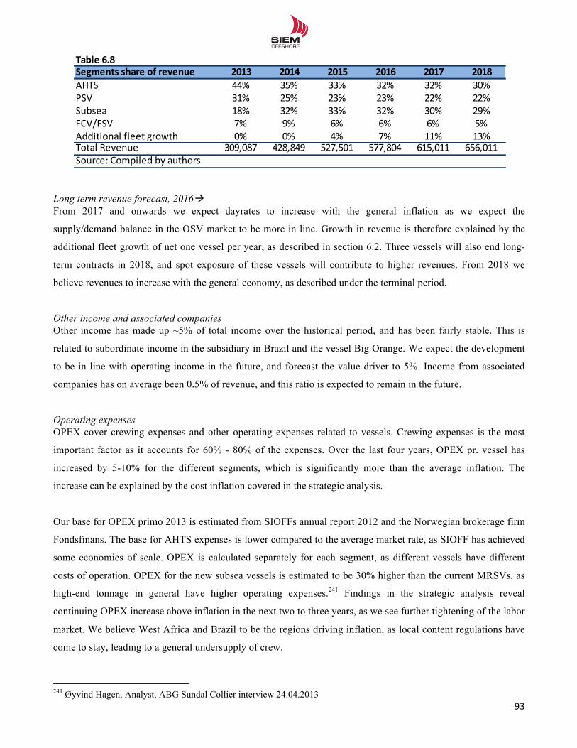
!!
93!!
Long term revenue forecast, 2016 From 2017 and onwards we expect dayrates to increase with the general inflation as we expect the
supply/demand balance in the OSV market to be more in line. Growth in revenue is therefore explained by the
additional fleet growth of net one vessel per year, as described in section 6.2. Three vessels will also end long-
term contracts in 2018, and spot exposure of these vessels will contribute to higher revenues. From 2018 we
believe revenues to increase with the general economy, as described under the terminal period.
Other income and associated companies Other income has made up ~5% of total income over the historical period, and has been fairly stable. This is
related to subordinate income in the subsidiary in Brazil and the vessel Big Orange. We expect the development
to be in line with operating income in the future, and forecast the value driver to 5%. Income from associated
companies has on average been 0.5% of revenue, and this ratio is expected to remain in the future.
Operating expenses OPEX cover crewing expenses and other operating expenses related to vessels. Crewing expenses is the most
important factor as it accounts for 60% - 80% of the expenses. Over the last four years, OPEX pr. vessel has
increased by 5-10% for the different segments, which is significantly more than the average inflation. The
increase can be explained by the cost inflation covered in the strategic analysis.
Our base for OPEX primo 2013 is estimated from SIOFFs annual report 2012 and the Norwegian brokerage firm
Fondsfinans. The base for AHTS expenses is lower compared to the average market rate, as SIOFF has achieved
some economies of scale. OPEX is calculated separately for each segment, as different vessels have different
costs of operation. OPEX for the new subsea vessels is estimated to be 30% higher than the current MRSVs, as
high-end tonnage in general have higher operating expenses.241 Findings in the strategic analysis reveal
continuing OPEX increase above inflation in the next two to three years, as we see further tightening of the labor
market. We believe West Africa and Brazil to be the regions driving inflation, as local content regulations have
come to stay, leading to a general undersupply of crew.
!!!!!!!!!!!!!!!!!!!!!!!!!!!!!!!!!!!!!!!!!!!!!!!!!!!!!!!!!!!!!241 Øyvind Hagen, Analyst, ABG Sundal Collier interview 24.04.2013
Table&6.8Segments&share&of&revenue 2013 2014 2015 2016 2017 2018AHTS 44% 35% 33% 32% 32% 30%PSV 31% 25% 23% 23% 22% 22%Subsea 18% 32% 33% 32% 30% 29%FCV/FSV 7% 9% 6% 6% 6% 5%Additional@fleet@growth 0% 0% 4% 7% 11% 13%Total@Revenue 309,087@ 428,849@ 527,501@ 577,804@ 615,011@ 656,011@Source:@Compiled@by@authors
!!
94!!
Vessels in other regions will also be affected by tightened market as offshore activity is expected to increase. In
2013 we expect OPEX inflation to be between 5-7 % for the different segments in addition to the general
inflation of 2.5%. This will gradually decline to 2-5% in 2014 as we see number of offshore deliveries to slowly
decline. We also believe SIOFF to have a good position in attracting crew with overweight of modern high-end
tonnage. We also believe that their Brazilian presence through subsidiary will be a strength to attract labor. From
2015 we therefore believe the situation to be more stable, forecasting OPEX to increase with the general inflation
of 2.5%. This is the inflation target used by industry professionals.242 OPEX for the FSV/FCV segment is
expected decrease by 5 % in 2013 and 10% in 2015, as new vessels are more efficient compared to older
tonnage. The complete OPEX forecast and the forecasted inflation can be seen in appendix 6.9.
In the forecasting period, OPEX in percent of revenue will decrease from 56% in 2013 to 48% in the terminal
period. Combined with the expected increase in revenue this will lead to margin expansion, bringing EBITDA
and EBIT-margin back to a more stable long term level.
Administration expenses Administration expenses has accounted for 11% of revenues historically. Over the last three years, expenses have
increased more than revenue and were 16% in 2012. The increase is a result of fleet expansion combined with
lower revenues. As the newbuilding program comes to an end, the organization is likely to operate more
efficiently. Going forward we believe administration expenses to increase at a decreasing pace, in line with
historical development. We expect the rate to be 14% in 2013, and decline to 11% by 2015.
Gain and losses from sale of fixed assets Gain/loss from sale of vessels has historically been below 5% of revenues, and has on average only accounted
for 0.6%. As SIOFF does not follow an asset play strategy, our best estimate is to forecast gain and losses in line
with the average historical development at 0.6%.243
Depreciation
The historical average depreciation rate has been 4.7%, which is equal to linear depreciation over ~21 years.
Vessels have an expected useful life of 25 years, while equipment/machinery has an average life of 7-15 years.
We therefore believe the historical depreciation is a good guide for the forecast period, setting it to 4.7% per
year.
Tax rate
We have applied the effective tax rate of 14% adjusted for deviation in 2011, as described in WACC at pg. 105.
!!!!!!!!!!!!!!!!!!!!!!!!!!!!!!!!!!!!!!!!!!!!!!!!!!!!!!!!!!!!!242 PwC (2012): “The Norwegian market risk premium 2012-2013” pg. 15 243 Plenborg & Petersen (2012) – Financial Statement Analysis pg. 203
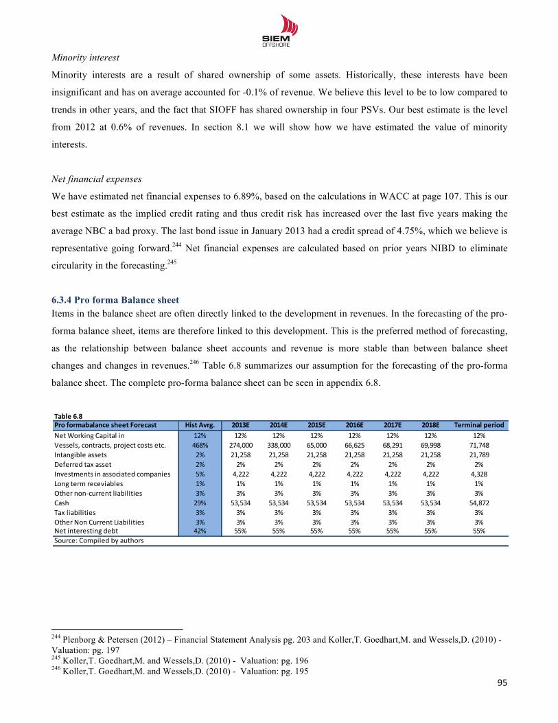
!!
95!!
Minority interest
Minority interests are a result of shared ownership of some assets. Historically, these interests have been
insignificant and has on average accounted for -0.1% of revenue. We believe this level to be to low compared to
trends in other years, and the fact that SIOFF has shared ownership in four PSVs. Our best estimate is the level
from 2012 at 0.6% of revenues. In section 8.1 we will show how we have estimated the value of minority
interests.
Net financial expenses
We have estimated net financial expenses to 6.89%, based on the calculations in WACC at page 107. This is our
best estimate as the implied credit rating and thus credit risk has increased over the last five years making the
average NBC a bad proxy. The last bond issue in January 2013 had a credit spread of 4.75%, which we believe is
representative going forward.244 Net financial expenses are calculated based on prior years NIBD to eliminate
circularity in the forecasting.245
6.3.4 Pro forma Balance sheet Items in the balance sheet are often directly linked to the development in revenues. In the forecasting of the pro-
forma balance sheet, items are therefore linked to this development. This is the preferred method of forecasting,
as the relationship between balance sheet accounts and revenue is more stable than between balance sheet
changes and changes in revenues.246 Table 6.8 summarizes our assumption for the forecasting of the pro-forma
balance sheet. The complete pro-forma balance sheet can be seen in appendix 6.8.
!!!!!!!!!!!!!!!!!!!!!!!!!!!!!!!!!!!!!!!!!!!!!!!!!!!!!!!!!!!!!244 Plenborg & Petersen (2012) – Financial Statement Analysis pg. 203 and Koller,T. Goedhart,M. and Wessels,D. (2010) - Valuation: pg. 197 245 Koller,T. Goedhart,M. and Wessels,D. (2010) - Valuation: pg. 196 246 Koller,T. Goedhart,M. and Wessels,D. (2010) - Valuation: pg. 195
Table&6.8Pro&formabalance&sheet&Forecast Hist&Avrg. 2013E 2014E 2015E 2016E 2017E 2018E Terminal&periodNet$Working$Capital$in 12% 12% 12% 12% 12% 12% 12% 12%Vessels,$contracts,$project$costs$etc. 468% 274,000$ 338,000$ 65,000$ 66,625$ 68,291$ 69,998$ 71,748$Intangible$assets 2% 21,258 21,258 21,258 21,258 21,258 21,258 21,789Deferred$tax$asset 2% 2% 2% 2% 2% 2% 2% 2%Investments$in$associated$companies 5% 4,222$ 4,222$ 4,222$ 4,222$ 4,222$ 4,222$ 4,328$Long$term$receviables 1% 1% 1% 1% 1% 1% 1% 1%Other$nonLcurrent$liabilities 3% 3% 3% 3% 3% 3% 3% 3%Cash 29% 53,534$ 53,534$ 53,534$ 53,534$ 53,534$ 53,534$ 54,872$Tax$liabilities 3% 3% 3% 3% 3% 3% 3% 3%Other$Non$Current$Liabilities 3% 3% 3% 3% 3% 3% 3% 3%Net$interesting$debt 42% 55% 55% 55% 55% 55% 55% 55%Source:$Compiled$by$authors
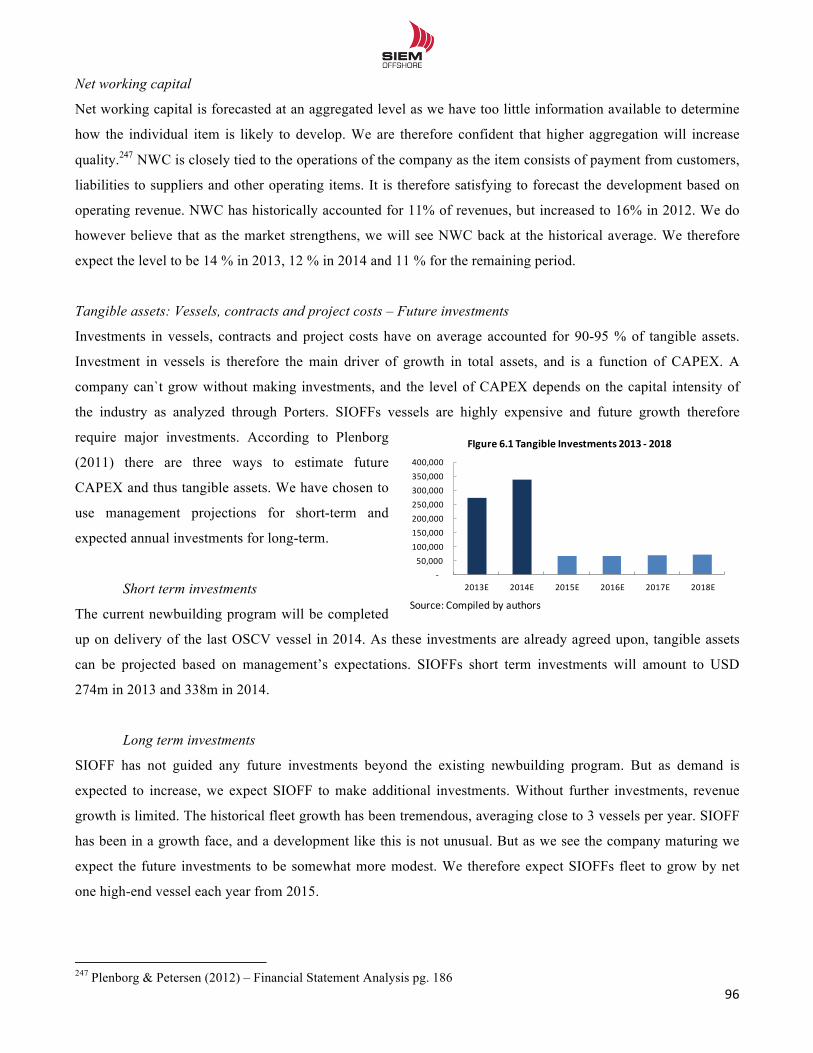
!!
96!!
Net working capital
Net working capital is forecasted at an aggregated level as we have too little information available to determine
how the individual item is likely to develop. We are therefore confident that higher aggregation will increase
quality.247 NWC is closely tied to the operations of the company as the item consists of payment from customers,
liabilities to suppliers and other operating items. It is therefore satisfying to forecast the development based on
operating revenue. NWC has historically accounted for 11% of revenues, but increased to 16% in 2012. We do
however believe that as the market strengthens, we will see NWC back at the historical average. We therefore
expect the level to be 14 % in 2013, 12 % in 2014 and 11 % for the remaining period.
Tangible assets: Vessels, contracts and project costs – Future investments
Investments in vessels, contracts and project costs have on average accounted for 90-95 % of tangible assets.
Investment in vessels is therefore the main driver of growth in total assets, and is a function of CAPEX. A
company can`t grow without making investments, and the level of CAPEX depends on the capital intensity of
the industry as analyzed through Porters. SIOFFs vessels are highly expensive and future growth therefore
require major investments. According to Plenborg
(2011) there are three ways to estimate future
CAPEX and thus tangible assets. We have chosen to
use management projections for short-term and
expected annual investments for long-term.
Short term investments
The current newbuilding program will be completed
up on delivery of the last OSCV vessel in 2014. As these investments are already agreed upon, tangible assets
can be projected based on management’s expectations. SIOFFs short term investments will amount to USD
274m in 2013 and 338m in 2014.
Long term investments
SIOFF has not guided any future investments beyond the existing newbuilding program. But as demand is
expected to increase, we expect SIOFF to make additional investments. Without further investments, revenue
growth is limited. The historical fleet growth has been tremendous, averaging close to 3 vessels per year. SIOFF
has been in a growth face, and a development like this is not unusual. But as we see the company maturing we
expect the future investments to be somewhat more modest. We therefore expect SIOFFs fleet to grow by net
one high-end vessel each year from 2015.
!!!!!!!!!!!!!!!!!!!!!!!!!!!!!!!!!!!!!!!!!!!!!!!!!!!!!!!!!!!!!247 Plenborg & Petersen (2012) – Financial Statement Analysis pg. 186
Source:(Compiled by(authors
550,000(100,000(150,000(200,000(250,000(300,000(350,000(400,000(
2013E 2014E 2015E 2016E 2017E 2018E
FIgure'6.1'Tangible'Investments'2013'8 2018
!!
97!!
As we have little information regarding the kind of vessel likely to be ordered, we expect investments reflecting
the average construction price across segments, estimated to USD 65m in 2015. Norwegian yards have currently
some bargaining power in the high-end segment, but Asian yards are likely to improve their skills. The
construction price of high-end vessels will therefore not increase significantly. We expect CAPEX to increase
with inflation, as illustrated in figure 6.1.
Other tangible assets and operating liabilities
Various balance sheet items have been estimated as percentage of revenue based on historical average, as this is
our best estimate for future development. Deferred tax asset has been forecasted at 2% of revenue. “Other long
term receivables” is based on the historical average of 2 %, and other “non-current liabilities” is based on the
average of 3%.
When it comes to investments in associated companies we do not expect SIOFF do make additional investments,
and base our forecast on the ultimo balance from 2012 of USD 4.2m. Operational stock of cash has fluctuated
historically, but we do not believe the future development will follow the revenue. Our forecast is therefore
identical to the current level at USD 53.5m.
Intangible assets
The item “intangible assets” is a result of the acquisition of Siem Offshore Contractors in 2011. There is no
information indicating that SIOFF will perform additional M&A activity, or that there is a need for impairment.
We assume that SIOFF only will grow organically, thus intangible assets will be constant at 21.3m through the
forecast period.248
Net Interest Bearing Debt
Net interest bearing debt is measured as a percentage of invested capital. The capital structure in the pro-forma
balance sheet should equal the capital structure implied by WACC.249 This is the long term capital structure as a
result of the iteration process in WACC. Therefore the expected level of net interest bearing debt is 54% of
invested capital, equal to WACC at pg. 106.
!!!!!!!!!!!!!!!!!!!!!!!!!!!!!!!!!!!!!!!!!!!!!!!!!!!!!!!!!!!!!248 Plenborg & Petersen (2012) – Financial Statement Analysis pg. 203 249 Koller,T. Goedhart,M. and Wessels,D. (2010) - Valuation: pg. 205
!!
98!!
6.3.5 Quality of the estimates supporting the pro forma statements To evaluate the validity of the pro forma statements it is important to look at the historical return and margins
against the forecasted performance. If the future performance deviates from the historical development, the
analyst needs strong arguments to support this view.250 The forecasted development is illustrated in figure 6.2.
SIOFFs ROIC has been declining since 2007 due to the weak market condition, as previously seen. This has also
affected the EBITDA-margin negatively. We believe the worst downturn to be behind us, and see strong support
for a positive development within the AHTS and Subsea segment going forward. Our forecasted EBITDA-
margin will therefore increase, but not to the same high level as seen in 2007. Consequently ROIC will increase
as well, reaching 10.1% in 2018, compared to 11.7% in 2007. Based on this development we believe there is a
strong validity in our forecast.
!!!!!!!!!!!!!!!!!!!!!!!!!!!!!!!!!!!!!!!!!!!!!!!!!!!!!!!!!!!!!250 Plenborg & Petersen (2012) – Financial Statement Analysis pg. 195
0.0%
10.0%
20.0%
30.0%
40.0%
50.0%
60.0%
2007 2008 2009 2010 2011 2012 2013 2014 2015 2016 2017 2018
Fiugre'6.2'Historical'vs.'forecasted'ROIC'and'EBITDA
ROIC EBITDA6margin
Source:6Compiled by6authors
!!
99!!
7.0 Estimating cost of capital To estimate the equity value of SIOFF using cash flow models, we must estimate a proper discount rate, known
as WACC. Equity- and debt holders demand a return of investment reflecting the risk of future cash flows. Debt
holders are normally entitled to a quarterly cash flow for a fixed period of time, and have priority in case of
default. The required rate of return must therefore be calculated separately for the two asset classes. The general
formula for WACC is illustrated below;251
!"## = !! ∗ 1 − ! ∗ !"#$!" + !! ∗!!"
7.1 Return on Equity, re To estimate the required rate of return of equity, there are several theoretical frameworks available. Most
financial literature (Plenborg, Koller mfl.) recommends using the general CAPM model, and we have therefore
chosen this model.252 This framework relies upon several theoretical assumptions, but an evaluation of these is
outside the scope of this thesis.253 SIOFF has only one equity class and we have thus estimated only one equity
return.
7.1.1 Risk free rate, rf The first element to estimate is the risk free interest rate. This rate is defined as an asset´s expected return with
certainty. To meet this condition the asset must have no default or reinvestment risk.254 The most widely used
proxy for the risk free rate is therefore a default free government bond with maturity matching the forecasting
horizon.255 To handle the issue of inflation it is important that the government bond is denominated in the same
currency as the underlying cash flow.256
SIOFFs cash flow is nominal and reported in USD, but the share price is quoted in NOK. To capture the effect of
inflation we therefore use the Norwegian risk free interest rate. Norway is recognized as one of the most solvent
nation in the world, and holds an AAA rating. There is thus zero default risk. As the forecasting horizon is
infinite, long term government bonds are preferred as proxy. To eliminate reinvestment risk, we therefore look at
10 - 30 year zero coupon bonds. Bonds with 30 year to maturity will best match the cash flow, but suffer from a
liquidity premium.257 Therefore it is not the preferred benchmark for the risk free rate. Based on 10 year zero
coupon bonds, we estimate the risk free rate to 2.14 % at the date of the analysis.258
!!!!!!!!!!!!!!!!!!!!!!!!!!!!!!!!!!!!!!!!!!!!!!!!!!!!!!!!!!!!!251 Plenborg & Petersen (2012) – Financial Statement Analysis pg. 246 252 re= rf + β*(rm – rf) 253 Pratt, P. Shannon (2002). Cost of Capital: Estimation and Applications 2th ed. pg. 77-78 254 Damodaran, Aswhat (2008), “What is the risk free rate? A search for the basic building block”, Pg. 6 255 Plenborg & Petersen (2012) – Financial Statement Analysis pg. 249 256 Plenborg & Petersen (2012) – Financial Statement Analysis pg. 251 257 Plenborg & Petersen (2012) – Financial Statement Analysis pg. 251 258 http://www.norges-bank.no/no/prisstabilitet/rentestatistikk/statsobligasjoner-rente-daglige-noteringer/
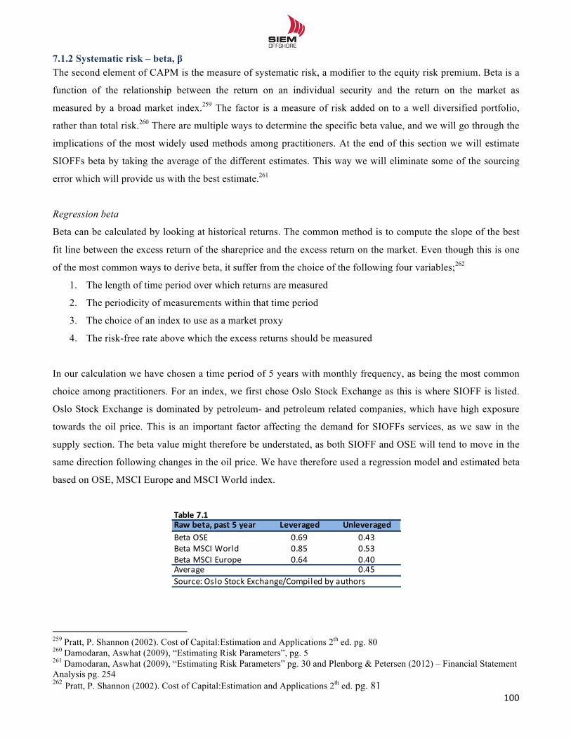
!!
100!!
7.1.2 Systematic risk – beta, β The second element of CAPM is the measure of systematic risk, a modifier to the equity risk premium. Beta is a
function of the relationship between the return on an individual security and the return on the market as
measured by a broad market index.259 The factor is a measure of risk added on to a well diversified portfolio,
rather than total risk.260 There are multiple ways to determine the specific beta value, and we will go through the
implications of the most widely used methods among practitioners. At the end of this section we will estimate
SIOFFs beta by taking the average of the different estimates. This way we will eliminate some of the sourcing
error which will provide us with the best estimate.261
Regression beta
Beta can be calculated by looking at historical returns. The common method is to compute the slope of the best
fit line between the excess return of the shareprice and the excess return on the market. Even though this is one
of the most common ways to derive beta, it suffer from the choice of the following four variables;262
1. The length of time period over which returns are measured
2. The periodicity of measurements within that time period
3. The choice of an index to use as a market proxy
4. The risk-free rate above which the excess returns should be measured
In our calculation we have chosen a time period of 5 years with monthly frequency, as being the most common
choice among practitioners. For an index, we first chose Oslo Stock Exchange as this is where SIOFF is listed.
Oslo Stock Exchange is dominated by petroleum- and petroleum related companies, which have high exposure
towards the oil price. This is an important factor affecting the demand for SIOFFs services, as we saw in the
supply section. The beta value might therefore be understated, as both SIOFF and OSE will tend to move in the
same direction following changes in the oil price. We have therefore used a regression model and estimated beta
based on OSE, MSCI Europe and MSCI World index.
!!!!!!!!!!!!!!!!!!!!!!!!!!!!!!!!!!!!!!!!!!!!!!!!!!!!!!!!!!!!!259 Pratt, P. Shannon (2002). Cost of Capital:Estimation and Applications 2th ed. pg. 80 260 Damodaran, Aswhat (2009), “Estimating Risk Parameters”, pg. 5 261 Damodaran, Aswhat (2009), “Estimating Risk Parameters” pg. 30 and Plenborg & Petersen (2012) – Financial Statement Analysis pg. 254 262 Pratt, P. Shannon (2002). Cost of Capital:Estimation and Applications 2th ed. pg. 81
Table&7.1Raw&beta,&past&5&year& Leveraged UnleveragedBeta%OSE 0.69 0.43Beta%MSCI%World 0.85 0.53Beta%MSCI%Europe 0.64 0.40Average 0.45Source:%Oslo%Stock%Exchange/Compiled%by%authors
!!
101!!
The first estimate is the leveraged beta, which is affected by the company`s capital structure over the historical
period. In the calculation of WACC we will use a beta value reflecting the future capital structure. We therefore
calculate the unleveraged beta by adjusting for the average NIBD/EV for the last five years.263 As can be seen
from table 7.1, the estimated betas based on historical return are low, indicating low systematic risk. This can be
plausible but might also be a result of low share liquidity.264 More than 50% of trading days have had a volume
below NOK 1 million, thus further analysis is necessary.
We have also computed beta values based on a seven year period, which can be seen in appendix 7.1. The beta
estimates are almost identical, and the deviation is insignificant.
Beta from comparable companies
One way to get beyond the problem of low liquidity is to use beta estimates from comparable companies.265 A
requirement of this method is that companies have the same risk profile. We have used beta estimates from
Reuters Financials for our peer group presented in section 2.10 These values have then been unleveraged to
eliminate the effect of capital structure.266 As appendix 7.2 illustrates, the average unleveraged beta is 0.38,
which is even lower than the regression estimates. Again liquidity is a major concern, as all these companies are
quite illiquid. Beta is also distorted by the financial gearing in Havila and DOF.
Industry beta
As the regression beta and betas from comparable firms have disadvantages, we look at a third way to estimate
the equity beta. This method is based on average beta for different industries, which is computed of researchers
such as Damodaran. In his 2012 beta-book he estimates an average industry beta of 1.09 based on 82 companies
in “Oil service/Equipment”. Compared to the regression and comparable firms, this method is based on a larger
dataset and has thus fewer sourcing errors.267
Beta from fundamental factors
The last approach suggested by theorists (Damodaran, Plenborg) is to estimate beta based on fundamental
factors. Through the strategic and financial analysis we have gained unique insights to the company´s operating
and financial position. By using this data, we have structured a risk assessment of the operating and financial
risk. Based on this analysis we have classified SIOFFs operating risk as High and the financial risk as Neutral.
!!!!!!!!!!!!!!!!!!!!!!!!!!!!!!!!!!!!!!!!!!!!!!!!!!!!!!!!!!!!!263 Pratt, P. Shannon (2002). Cost of Capital:Estimation and Applications 2th ed. pg. 84 264 Plenborg & Petersen (2012) – Financial Statement Analysis pg. 252 265 Plenborg & Petersen (2012) – Financial Statement Analysis pg. 254 266 Pratt, P. Shannon (2002). Cost of Capital:Estimation and Applications 2th ed. pg. 275 267 Damodaran, Aswhat (2012), Dataset – Industry beta values
!!
102!!
The overall risk is therefore classified as high, which implies an unleveraged beta between 1.15-1.4.268 We have
therefore applied a fundamental beta of 1.25. The analysis can be seen in appendix 7.3
Unleveraged beta estimate
Based on the different theoretical approaches we have estimated an unleveraged beta value in the range from
0.38 to 1.25. This is a wide span reflecting possible estimation errors. To reduce the impact of errors we have
calculated the average of all the observations. The unleveraged beta value applicable for SIOFF is thus 0.79. This
is a more plausible estimate compared to the output from the regression, as the OSV industry is a cyclical
business with perceived risk higher than what a beta value of 0.38 can explain.
In the long run, beta has a tendency to converge towards the market average of one. Bloomberg has developed a
method to adjust for this tendency, and the adjusted beta is 0.86.269
7.1.3 Equity risk premium The equity risk premium is calculated ex-post based on the historical excess return on the stock market over the
risk free rate, and varies over time. The most common way to estimate this measure is with references to books
and articles.270 Brealey and Meyers (2008) suggest an equity risk premium of 7.6%.271 Koller et. Al. estimates the
premium to be in the range from 4.5 – 5.5%.272 In addition, professor Damodaran estimates the premium to be
5.7%. This is also supported by professor Fernandéz (2012), who estimate the premium to 5.8%.273 We have
chosen to use Damodaran as source, as his estimates are continuously updated and lies between the other
estimates. The risk premium is set at 5.7 %.274
7.1.4 Liquidity premium The last factor of the equity premium is a premium for illiquidity. This premium refers to the costs and problem
of converting stocks or other assets to cash. SIOFFs trading volume is low, as previously mentioned, and there
can be some problems associated with transaction of stocks. To solve for this problem, researchers (Plenborg,
Petersen, and Pratt) finds that investors adjust their rate of return by 3-5 %.275 This is supported by an annual
survey from PwC for the Norwegian market, where 81% (of 178 respondents) apply a small stock premium.276
We have therefore added a liquidity premium of 3 % to the final estimate of the equity return.
!!!!!!!!!!!!!!!!!!!!!!!!!!!!!!!!!!!!!!!!!!!!!!!!!!!!!!!!!!!!!268 Plenborg & Petersen (2012) – Financial Statement Analysis pg. 262 269 Koller,T. Goedhart,M. and Wessels,D. (2010) - Valuation: pg. 253 270 Plenborg & Petersen (2012) – Financial Statement Analysis pg. 264 271 Brealey, A., Myers, S., Allen, F., (2008). Principles of corporate finance. 9th ed. pg. 215 272 Koller,T. Goedhart,M. and Wessels,D. (2010) - Valuation: pg. 236 273 PwC (2012): “The Norwegian market risk premium 2012-2013”, pg.11 274 Damodaran (2012): Dataset: Risk premium for other markets 275 Plenborg & Petersen (2012) – Financial Statement Analysis pg. 265, Pratt, P. Shannon (2002). Cost of Capital: Estimation and Applications 2th ed. pg. 77 276 PwC (2012): “The Norwegian market risk premium 2012-2013”, pg.13
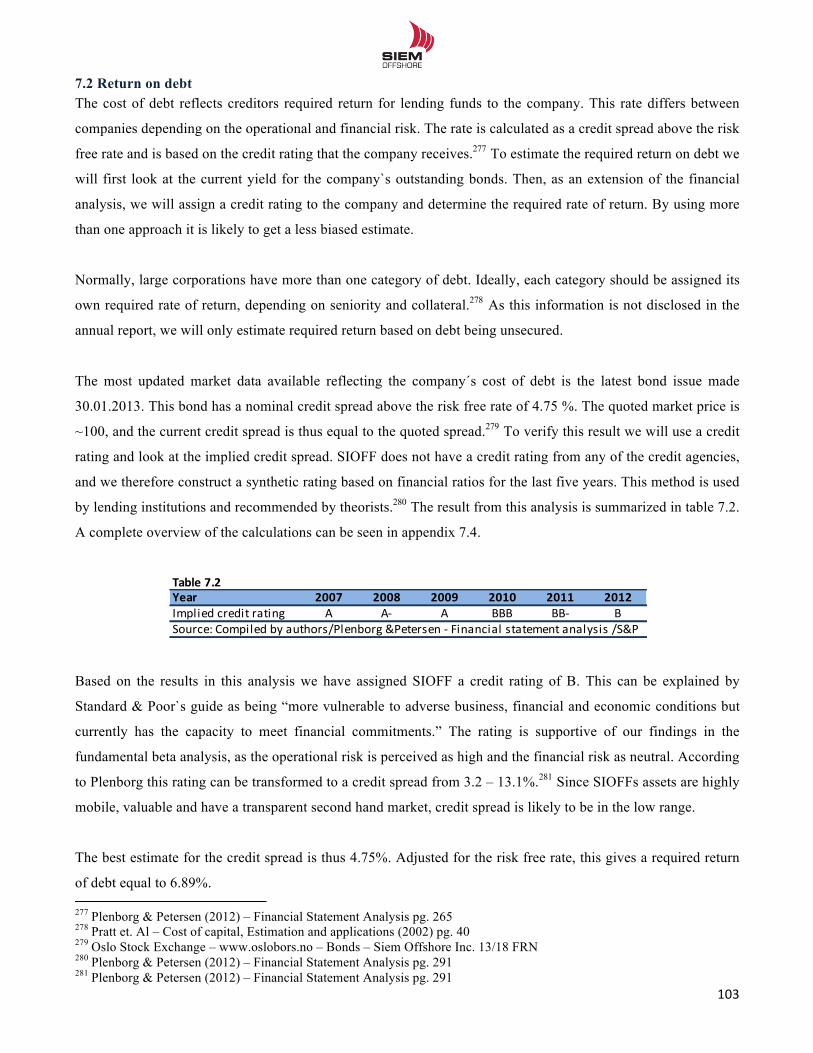
!!
103!!
7.2 Return on debt The cost of debt reflects creditors required return for lending funds to the company. This rate differs between
companies depending on the operational and financial risk. The rate is calculated as a credit spread above the risk
free rate and is based on the credit rating that the company receives.277 To estimate the required return on debt we
will first look at the current yield for the company`s outstanding bonds. Then, as an extension of the financial
analysis, we will assign a credit rating to the company and determine the required rate of return. By using more
than one approach it is likely to get a less biased estimate.
Normally, large corporations have more than one category of debt. Ideally, each category should be assigned its
own required rate of return, depending on seniority and collateral.278 As this information is not disclosed in the
annual report, we will only estimate required return based on debt being unsecured.
The most updated market data available reflecting the company´s cost of debt is the latest bond issue made
30.01.2013. This bond has a nominal credit spread above the risk free rate of 4.75 %. The quoted market price is
~100, and the current credit spread is thus equal to the quoted spread.279 To verify this result we will use a credit
rating and look at the implied credit spread. SIOFF does not have a credit rating from any of the credit agencies,
and we therefore construct a synthetic rating based on financial ratios for the last five years. This method is used
by lending institutions and recommended by theorists.280 The result from this analysis is summarized in table 7.2.
A complete overview of the calculations can be seen in appendix 7.4.
Based on the results in this analysis we have assigned SIOFF a credit rating of B. This can be explained by
Standard & Poor`s guide as being “more vulnerable to adverse business, financial and economic conditions but
currently has the capacity to meet financial commitments.” The rating is supportive of our findings in the
fundamental beta analysis, as the operational risk is perceived as high and the financial risk as neutral. According
to Plenborg this rating can be transformed to a credit spread from 3.2 – 13.1%.281 Since SIOFFs assets are highly
mobile, valuable and have a transparent second hand market, credit spread is likely to be in the low range.
The best estimate for the credit spread is thus 4.75%. Adjusted for the risk free rate, this gives a required return
of debt equal to 6.89%. !!!!!!!!!!!!!!!!!!!!!!!!!!!!!!!!!!!!!!!!!!!!!!!!!!!!!!!!!!!!!277 Plenborg & Petersen (2012) – Financial Statement Analysis pg. 265 278 Pratt et. Al – Cost of capital, Estimation and applications (2002) pg. 40 279 Oslo Stock Exchange – www.oslobors.no – Bonds – Siem Offshore Inc. 13/18 FRN 280 Plenborg & Petersen (2012) – Financial Statement Analysis pg. 291 281 Plenborg & Petersen (2012) – Financial Statement Analysis pg. 291
Table&7.2Year 2007 2008 2009 2010 2011 2012Implied(credit(rating A A0 A BBB BB0 BSource:(Compiled(by(authors/Plenborg(&Petersen(0(Financial(statement(analysis(/S&P
!!
104!!
Tax rate
Since free cash flow is calculated in after tax terms, we must adjust the cost of capital reflecting the fact that
interest costs are deductible. SIOFF has operations across many geographical regions and are thus subject to
different tax rate regimes. Applying the Norwegian corporate tax rate is therefore inconvenient. The best
estimate for the corporate tax rate is therefore the effective tax rate from the financial statement. We base our
estimate on the historical average tax rate, adjusted for the extreme deviation in 2011. It is important to notice
that this method suffer from a drawback, since it assume that that borrowing costs are distributed in the same
way as operating earnings.282 The implication for SIOFF is less obvious as the company has borrowings in three
different regions and currencies.
The corporate tax rate is therefore set to be 14%.
7.3 Capital structure The last stage in estimation of WACC is the capital structure of debt and equity. To estimate these values it is
important to rely on market values, as WACC represents the expected return on an alternative investment with
identical risk. Book values therefore represent a historical cost.283
One approach is to estimate a target debt ratio for the firm, by subtracting current value of debt from enterprise
value to get equity value. This method gives the correct equity value in situations where the debt ratio will move
towards a determined target ratio. This is the appropriate method for corporate takeovers and capital budgeting.
In this thesis we estimate the fundamental value of a marginal share in SIOFF. This is considered as a passive
investment where the shareholder is unlikely to influence the level of debt. In practice, future cash flow of the
company will affect the debt ratio and these cash flows are estimated with a degree of uncertainty. It is therefore
meaningless to apply a target debt ratio, when this ratio is determined by the future cash flow. Estimating equity
value in a passive investment should rather be based on the forecasted equity value as the target debt level is
unknown. To correct for circularity we will therefore apply an iterative procedure.284
We start the procedure by estimating the current market value of debt. The market value of debt is not
transparent, as there are few disclosures in the annual report. As SIOFF is in a healthy financial position with few
fixed-rate borrowings, the market value of the listed bond described in section 7.2 can be used as guideline. As
the market value is close to 100, book value of debt is a reasonable approximation.
!!!!!!!!!!!!!!!!!!!!!!!!!!!!!!!!!!!!!!!!!!!!!!!!!!!!!!!!!!!!!282 Plenborg & Petersen (2012) – Financial Statement Analysis pg. 265 283 Koller,T. Goedhart,M. and Wessels,D. (2010) - Valuation: pg. 262 284 Patrick Larkin (2011): “To Iterate or not to iterate? Using the WACC in equity valuation” pg. 1-2
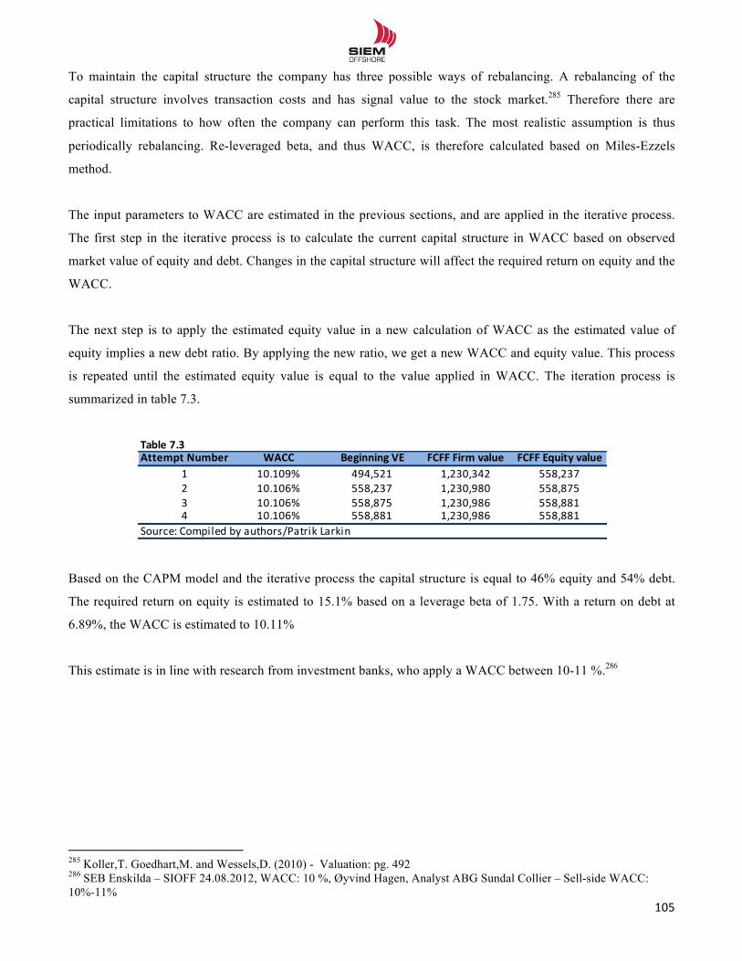
!!
105!!
To maintain the capital structure the company has three possible ways of rebalancing. A rebalancing of the
capital structure involves transaction costs and has signal value to the stock market.285 Therefore there are
practical limitations to how often the company can perform this task. The most realistic assumption is thus
periodically rebalancing. Re-leveraged beta, and thus WACC, is therefore calculated based on Miles-Ezzels
method.
The input parameters to WACC are estimated in the previous sections, and are applied in the iterative process.
The first step in the iterative process is to calculate the current capital structure in WACC based on observed
market value of equity and debt. Changes in the capital structure will affect the required return on equity and the
WACC.
The next step is to apply the estimated equity value in a new calculation of WACC as the estimated value of
equity implies a new debt ratio. By applying the new ratio, we get a new WACC and equity value. This process
is repeated until the estimated equity value is equal to the value applied in WACC. The iteration process is
summarized in table 7.3.
Based on the CAPM model and the iterative process the capital structure is equal to 46% equity and 54% debt.
The required return on equity is estimated to 15.1% based on a leverage beta of 1.75. With a return on debt at
6.89%, the WACC is estimated to 10.11%
This estimate is in line with research from investment banks, who apply a WACC between 10-11 %.286
!
!!!!!!!!!!!!!!!!!!!!!!!!!!!!!!!!!!!!!!!!!!!!!!!!!!!!!!!!!!!!!285 Koller,T. Goedhart,M. and Wessels,D. (2010) - Valuation: pg. 492 286 SEB Enskilda – SIOFF 24.08.2012, WACC: 10 %, Øyvind Hagen, Analyst ABG Sundal Collier – Sell-side WACC: 10%-11%
Table&7.3Attempt&Number WACC Beginning&VE FCFF&Firm&value FCFF&Equity&value
1 10.109% 494,521* 1,230,342* 558,237*2 10.106% 558,237* 1,230,980* 558,875*3 10.106% 558,875* 1,230,986* 558,881*4 10.106% 558,881* 1,230,986* 558,881*
Source:*Compiled*by*authors/Patrik*Larkin
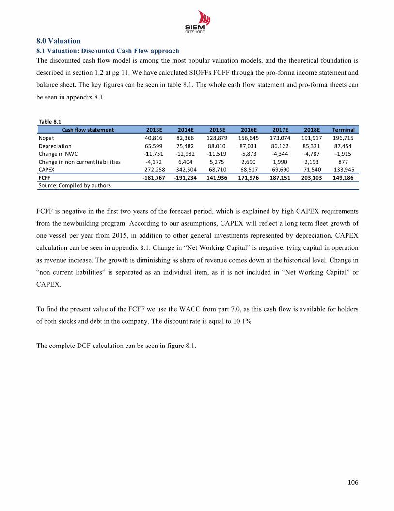
!!
106!!
8.0 Valuation 8.1 Valuation: Discounted Cash Flow approach The discounted cash flow model is among the most popular valuation models, and the theoretical foundation is
described in section 1.2 at pg 11. We have calculated SIOFFs FCFF through the pro-forma income statement and
balance sheet. The key figures can be seen in table 8.1. The whole cash flow statement and pro-forma sheets can
be seen in appendix 8.1.
FCFF is negative in the first two years of the forecast period, which is explained by high CAPEX requirements
from the newbuilding program. According to our assumptions, CAPEX will reflect a long term fleet growth of
one vessel per year from 2015, in addition to other general investments represented by depreciation. CAPEX
calculation can be seen in appendix 8.1. Change in “Net Working Capital” is negative, tying capital in operation
as revenue increase. The growth is diminishing as share of revenue comes down at the historical level. Change in
“non current liabilities” is separated as an individual item, as it is not included in “Net Working Capital” or
CAPEX.
To find the present value of the FCFF we use the WACC from part 7.0, as this cash flow is available for holders
of both stocks and debt in the company. The discount rate is equal to 10.1%
The complete DCF calculation can be seen in figure 8.1.
Table&8.1Cash&flow&statement 2013E 2014E 2015E 2016E 2017E 2018E Terminal
Nopat 40,816 82,366 128,879 156,645 173,074 191,917 196,715Depreciation 65,599 75,482 88,010 87,031 86,122 85,321 87,454Change:in:NWC <11,751 <12,982 <11,519 <5,873 <4,344 <4,787 <1,915Change:in:non:current:l iabilities <4,172 6,404 5,275 2,690 1,990 2,193 877CAPEX <272,258 <342,504 <68,710 <68,517 <69,690 <71,540 <133,945FCFF >181,767 >191,234 141,936 171,976 187,151 203,103 149,186Source::Compiled:by:authors
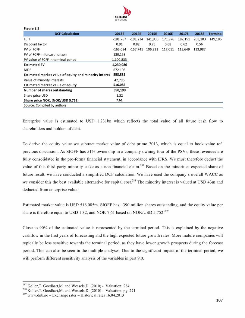
!!
107!!
Enterprise value is estimated to USD 1.231bn which reflects the total value of all future cash flow to
shareholders and holders of debt.
To derive the equity value we subtract market value of debt primo 2013, which is equal to book value ref.
previous discussion. As SIOFF has 51% ownership in a company owning four of the PSVs, these revenues are
fully consolidated in the pro-forma financial statement, in accordance with IFRS. We must therefore deduct the
value of this third party minority stake as a non-financial claim.287 Based on the minorities expected share of
future result, we have conducted a simplified DCF calculation. We have used the company´s overall WACC as
we consider this the best available alternative for capital cost.288 The minority interest is valued at USD 43m and
deducted from enterprise value.
Estimated market value is USD 516.085m. SIOFF has ~390 million shares outstanding, and the equity value per
share is therefore equal to USD 1.32, and NOK 7.61 based on NOK/USD 5.752.289
Close to 90% of the estimated value is represented by the terminal period. This is explained by the negative
cashflow in the first years of forecasting and the high expected future growth rates. More mature companies will
typically be less sensitive towards the terminal period, as they have lower growth prospects during the forecast
period. This can also be seen in the multiple analyses. Due to the significant impact of the terminal period, we
will perform different sensitivity analysis of the variables in part 9.0.
!!!!!!!!!!!!!!!!!!!!!!!!!!!!!!!!!!!!!!!!!!!!!!!!!!!!!!!!!!!!!287 Koller,T. Goedhart,M. and Wessels,D. (2010) - Valuation: 284 288 Koller,T. Goedhart,M. and Wessels,D. (2010) - Valuation: pg. 271 289 www.dnb.no – Exchange rates – Historical rates 16.04.2013
Figure'8.1DCF'Calculation 2013E 2014E 2015E 2016E 2017E 2018E Terminal
FCFF #181,767 #191,234 141,936 171,976 187,151 203,103 149,186Discount7factor 0.91 0.82 0.75 0.68 0.62 0.56PV7of7FCFF #165,084 #157,741 106,331 117,011 115,649 113,987PV7of7FCFF7in7forcast7horizon 130,153PV7value7of7FCFF7in7terminal7period 1,100,833Estimated'EV 1,230,986NIDB 672,105Estimated'market'value'of'equity'and'minority'interests558,881Value7of7minority7interests 42,796Estimated'market'value'of'equity 516,085Number'of'shares'outstanding 390,190Share7price7USD 1.32Share'price'NOK,'(NOK/USD'5.752) 7.61Source:7Compiled7by7authors
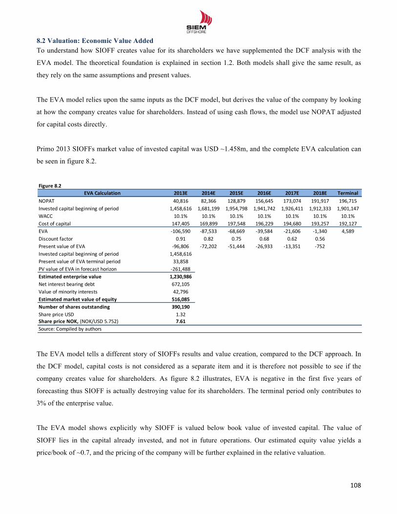
!!
108!!
8.2 Valuation: Economic Value Added To understand how SIOFF creates value for its shareholders we have supplemented the DCF analysis with the
EVA model. The theoretical foundation is explained in section 1.2. Both models shall give the same result, as
they rely on the same assumptions and present values.
The EVA model relies upon the same inputs as the DCF model, but derives the value of the company by looking
at how the company creates value for shareholders. Instead of using cash flows, the model use NOPAT adjusted
for capital costs directly.
Primo 2013 SIOFFs market value of invested capital was USD ~1.458m, and the complete EVA calculation can
be seen in figure 8.2.
The EVA model tells a different story of SIOFFs results and value creation, compared to the DCF approach. In
the DCF model, capital costs is not considered as a separate item and it is therefore not possible to see if the
company creates value for shareholders. As figure 8.2 illustrates, EVA is negative in the first five years of
forecasting thus SIOFF is actually destroying value for its shareholders. The terminal period only contributes to
3% of the enterprise value.
The EVA model shows explicitly why SIOFF is valued below book value of invested capital. The value of
SIOFF lies in the capital already invested, and not in future operations. Our estimated equity value yields a
price/book of ~0.7, and the pricing of the company will be further explained in the relative valuation.
Figure'8.2EVA'Calculation 2013E 2014E 2015E 2016E 2017E 2018E Terminal
NOPAT 40,816 82,366 128,879 156,645 173,074 191,917 196,715Invested8capital8beginning8of8period 1,458,616 1,681,199 1,954,798 1,941,742 1,926,411 1,912,333 1,901,147WACC 10.1% 10.1% 10.1% 10.1% 10.1% 10.1% 10.1%Cost8of8capital 147,405 169,899 197,548 196,229 194,680 193,257 192,127EVA I106,590 I87,533 I68,669 I39,584 I21,606 I1,340 4,589Discount8factor 0.91 0.82 0.75 0.68 0.62 0.56Present8value8of8EVA I96,806 I72,202 I51,444 I26,933 I13,351 I752Invested8capital8beginning8of8period 1,458,616Present8value8of8EVA8terminal8period 33,858 8PV8value8of8EVA8in8forecast8horizon I261,488Estimated'enterprise'value 1,230,986Net8interest8bearing8debt 672,105Value8of8minority8interests 42,796Estimated'market'value'of'equity 516,085Number'of'shares'outstanding 390,190Share8price8USD 1.32Share'price'NOK,'(NOK/USD85.752) 7.61Source:8Compiled8by8authors
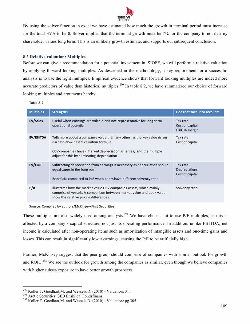
!!
109!!
By using the solver function in excel we have estimated how much the growth in terminal period must increase
for the total EVA to be 0. Solver implies that the terminal growth must be 7% for the company to not destroy
shareholder values long term. This is an unlikely growth estimate, and supports our subsequent conclusion.
8.3 Relative valuation: Multiples Before we can give a recommendation for a potential investment in SIOFF, we will perform a relative valuation
by applying forward looking multiples. As described in the methodology, a key requirement for a successful
analysis is to use the right multiples. Empirical evidence shows that forward looking multiples are indeed more
accurate predictors of value than historical multiples.290 In table 8.2, we have summarized our choice of forward
looking multiples and arguments hereby.
These multiples are also widely used among analysts.291 We have chosen not to use P/E multiples, as this is
affected by a company´s capital structure, not just its operating performance. In addition, unlike EBITDA, net
income is calculated after non-operating items such as amortization of intangible assets and one-time gains and
losses. This can result in significantly lower earnings, causing the P/E to be artificially high.
Further, McKinsey suggest that the peer group should comprise of companies with similar outlook for growth
and ROIC.292 We see the outlook for growth among the companies as similar, even though we believe companies
with higher subsea exposure to have better growth prospects.
!!!!!!!!!!!!!!!!!!!!!!!!!!!!!!!!!!!!!!!!!!!!!!!!!!!!!!!!!!!!!290 Koller,T. Goedhart,M. and Wessels,D. (2010) - Valuation: 311 291 Arctic Securities, SEB Enskilda, Fondsfinans 292 Koller,T. Goedhart,M. and Wessels,D. (2010) - Valuation: pg 305
Multiples Strengths Does0not0take0into account:
EV/Sales Usefulwhen earnings are volatile and2not2representative for2long4termoperational potential
Tax rateCost of2capitalEBITDA2margin
EV/EBITDA Tells2more2about2a2companys value2than2any2other,2as2the2key2value2driver2is2a2cash4flow4based2valuation2formula
OSV2companies2have2different2depreciation2schemes,22and2the2multiple2adjust2for2this2by2eliminating2 depreciation
Tax rateCost2of2capital
EV/EBIT Subtracting2depreciation2from2earnings2is2necessary2as2depreciation2should2equal2capex in2the2long2run
Beneficial2compared2to2P/E2when2peers2have2different2solvency2ratio
Tax rateDepreciationsCost2of2capital
P/B Illustrates how the2market value OSV2companies assets,2which mainlycomprise of2vessels.2A2comparison between market value and2book2valueshow2the2relative2pricingdifferences.
Solvency ratio
Table 8.2
Source:2Compiled by2authors/McKinsey/First Securities
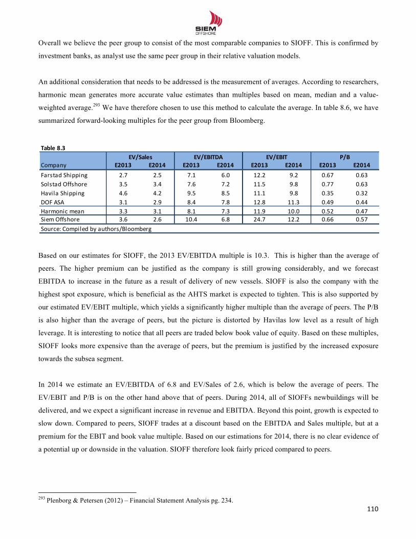
!!
110!!
Overall we believe the peer group to consist of the most comparable companies to SIOFF. This is confirmed by
investment banks, as analyst use the same peer group in their relative valuation models.
An additional consideration that needs to be addressed is the measurement of averages. According to researchers,
harmonic mean generates more accurate value estimates than multiples based on mean, median and a value-
weighted average.293 We have therefore chosen to use this method to calculate the average. In table 8.6, we have
summarized forward-looking multiples for the peer group from Bloomberg.
Based on our estimates for SIOFF, the 2013 EV/EBITDA multiple is 10.3. This is higher than the average of
peers. The higher premium can be justified as the company is still growing considerably, and we forecast
EBITDA to increase in the future as a result of delivery of new vessels. SIOFF is also the company with the
highest spot exposure, which is beneficial as the AHTS market is expected to tighten. This is also supported by
our estimated EV/EBIT multiple, which yields a significantly higher multiple than the average of peers. The P/B
is also higher than the average of peers, but the picture is distorted by Havilas low level as a result of high
leverage. It is interesting to notice that all peers are traded below book value of equity. Based on these multiples,
SIOFF looks more expensive than the average of peers, but the premium is justified by the increased exposure
towards the subsea segment.
In 2014 we estimate an EV/EBITDA of 6.8 and EV/Sales of 2.6, which is below the average of peers. The
EV/EBIT and P/B is on the other hand above that of peers. During 2014, all of SIOFFs newbuildings will be
delivered, and we expect a significant increase in revenue and EBITDA. Beyond this point, growth is expected to
slow down. Compared to peers, SIOFF trades at a discount based on the EBITDA and Sales multiple, but at a
premium for the EBIT and book value multiple. Based on our estimations for 2014, there is no clear evidence of
a potential up or downside in the valuation. SIOFF therefore look fairly priced compared to peers.
!!!!!!!!!!!!!!!!!!!!!!!!!!!!!!!!!!!!!!!!!!!!!!!!!!!!!!!!!!!!!293 Plenborg & Petersen (2012) – Financial Statement Analysis pg. 234.
Table&8.3
Company E2013 E2014 E2013 E2014 E2013 E2014 E2013 E2014Farstad-Shipping 2.7 2.5 7.1 6.0 12.2 9.2 0.67 0.63Solstad-Offshore 3.5 3.4 7.6 7.2 11.5 9.8 0.77 0.63Havila-Shipping 4.6 4.2 9.5 8.5 11.1 9.8 0.35 0.32DOF-ASA 3.1 2.9 8.4 7.8 12.8 11.3 0.49 0.44Harmonic-mean 3.3 3.1 8.1 7.3 11.9 10.0 0.52 0.47Siem-Offshore 3.6 2.6 10.4 6.8 24.7 12.2 0.66 0.57
P/BEV/EBITEV/EBITDAEV/Sales
Source:-Compiled-by-authors/Bloomberg
!!
111!!
We have also compared our estimated multiples with consensus estimates for SIOFF from Bloomberg.
Compared to consensus seen in appendix 8.2, all our forecasted values are below average. The difference can be
explained by our lower estimates of revenue and EBITDA, and we consider the company to be more expensive
than the opinions of analysts. This can possibly indicate that our estimates are conservative, and be a sign of a
potential upside of the valuation. However, compared to the historical EBITDA-margin and ROIC illustrated at
page 99, we believe our forecast is more reliable. In our forecast we project an increasing demand for OSV
services, in line with analysts’ opinion. However, we see the supply side increasing as well, limiting the potential
upside of dayrates. In the following section, we will discuss our underlying assumptions.
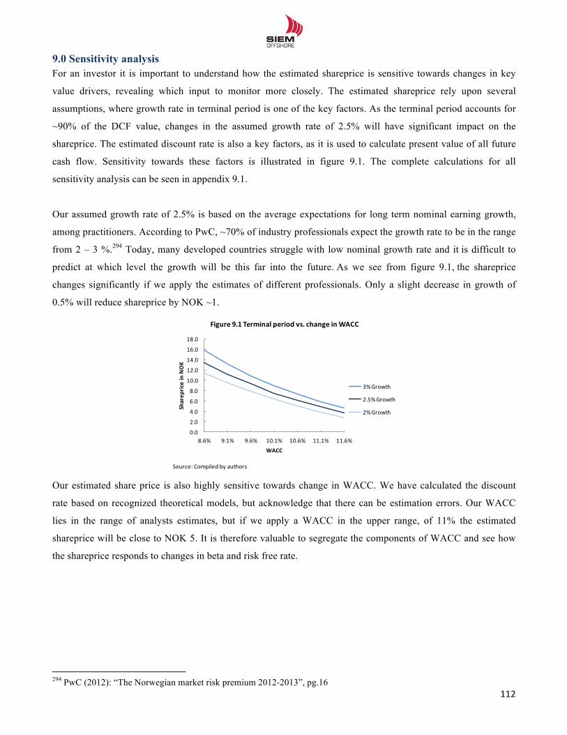
!!
112!!
9.0 Sensitivity analysis For an investor it is important to understand how the estimated shareprice is sensitive towards changes in key
value drivers, revealing which input to monitor more closely. The estimated shareprice rely upon several
assumptions, where growth rate in terminal period is one of the key factors. As the terminal period accounts for
~90% of the DCF value, changes in the assumed growth rate of 2.5% will have significant impact on the
shareprice. The estimated discount rate is also a key factors, as it is used to calculate present value of all future
cash flow. Sensitivity towards these factors is illustrated in figure 9.1. The complete calculations for all
sensitivity analysis can be seen in appendix 9.1.
Our assumed growth rate of 2.5% is based on the average expectations for long term nominal earning growth,
among practitioners. According to PwC, ~70% of industry professionals expect the growth rate to be in the range
from 2 – 3 %.294 Today, many developed countries struggle with low nominal growth rate and it is difficult to
predict at which level the growth will be this far into the future. As we see from figure 9.1, the shareprice
changes significantly if we apply the estimates of different professionals. Only a slight decrease in growth of
0.5% will reduce shareprice by NOK ~1.
Our estimated share price is also highly sensitive towards change in WACC. We have calculated the discount
rate based on recognized theoretical models, but acknowledge that there can be estimation errors. Our WACC
lies in the range of analysts estimates, but if we apply a WACC in the upper range, of 11% the estimated
shareprice will be close to NOK 5. It is therefore valuable to segregate the components of WACC and see how
the shareprice responds to changes in beta and risk free rate.
!!!!!!!!!!!!!!!!!!!!!!!!!!!!!!!!!!!!!!!!!!!!!!!!!!!!!!!!!!!!!294 PwC (2012): “The Norwegian market risk premium 2012-2013”, pg.16
0.0
2.0
4.0
6.0
8.0
10.0
12.0
14.0
16.0
18.0
8.6% 9.1% 9.6% 10.1% 10.6% 11.1% 11.6%
Sharep
rice)in)NOK
WACC
Figure)9.1)Terminal)period)vs.)change)in)WACC
3%+Growth
2.5%+Growth
2%+Growth
Source:+Compiled by+authors
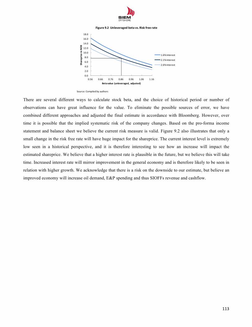
!!
113!!
There are several different ways to calculate stock beta, and the choice of historical period or number of
observations can have great influence for the value. To eliminate the possible sources of error, we have
combined different approaches and adjusted the final estimate in accordance with Bloomberg. However, over
time it is possible that the implied systematic risk of the company changes. Based on the pro-forma income
statement and balance sheet we believe the current risk measure is valid. Figure 9.2 also illustrates that only a
small change in the risk free rate will have huge impact for the shareprice. The current interest level is extremely
low seen in a historical perspective, and it is therefore interesting to see how an increase will impact the
estimated shareprice. We believe that a higher interest rate is plausible in the future, but we believe this will take
time. Increased interest rate will mirror improvement in the general economy and is therefore likely to be seen in
relation with higher growth. We acknowledge that there is a risk on the downside to our estimate, but believe an
improved economy will increase oil demand, E&P spending and thus SIOFFs revenue and cashflow.
Source:(Compiled by(authors
0.0
2.0
4.0
6.0
8.0
10.0
12.0
14.0
16.0
18.0
0.56( 0.66( 0.76( 0.86( 0.96( 1.06( 1.16(Sharep
rice)in)NOK
Beta)value)(unleveraged,) adjusted)
Figure)9.2))Unleveraged)beta)vs.)Risk)free)rate
1.6%(Interest
2.1%(Interest
2.6%(Interest
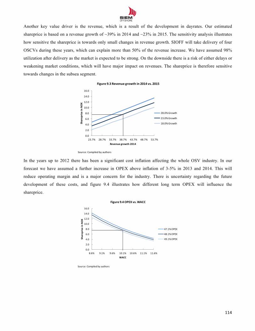
!!
114!!
Another key value driver is the revenue, which is a result of the development in dayrates. Our estimated
shareprice is based on a revenue growth of ~39% in 2014 and ~23% in 2015. The sensitivity analysis illustrates
how sensitive the shareprice is towards only small changes in revenue growth. SIOFF will take delivery of four
OSCVs during these years, which can explain more than 50% of the revenue increase. We have assumed 98%
utilization after delivery as the market is expected to be strong. On the downside there is a risk of either delays or
weakening market conditions, which will have major impact on revenues. The shareprice is therefore sensitive
towards changes in the subsea segment.
In the years up to 2012 there has been a significant cost inflation affecting the whole OSV industry. In our
forecast we have assumed a further increase in OPEX above inflation of 3-5% in 2013 and 2014. This will
reduce operating margin and is a major concern for the industry. There is uncertainty regarding the future
development of these costs, and figure 9.4 illustrates how different long term OPEX will influence the
shareprice.
Source:(Compiled by(authors
0.0
2.0
4.0
6.0
8.0
10.0
12.0
14.0
16.0
23.7% 28.7% 33.7% 38.7% 43.7% 48.7% 53.7%
Sharep
rice)in)NOK
Revenue)growth)2014
Figure)9.3)Revenue)growth)in)2014)vs.)2015
28.0%(Growth
23.0%(Growth
18.0%(Growth
Source:(Compiled by(authors
0.0
2.0
4.0
6.0
8.0
10.0
12.0
14.0
16.0
8.6% 9.1% 9.6% 10.1% 10.6% 11.1% 11.6%
Sharep
rice)in)NOK
WACC
Figure)9.4)OPEX)vs.)WACC
47.1%(OPEX
48.1%(OPEX
49.1%(OPEX
!!
115!!
9.1 Partial conclusion
The 16th of April 2013 SIOFFs shares were traded at NOK 7.29. Compared to our DCF estimate of NOK 7.6,
this represents a potential upside of 4%. However, the estimated price must be seen in context to the EVA model,
multiple valuations and the sensitivity analysis.
The result from the EVA model showed that the company is destroying value for shareholders during the first
years of the forecast horizon, and that the value of SIOFF is reflected in the current fleet of vessels. This is
further confirmed by the multiple analyses, where P/B is well below 1. For 2013 multiples, SIOFF looks
somewhat higher priced compared to peers. This is explained by the newbuilding program and the expected
improvement in dayrates. In 2014, SIOFF looks fairly priced. This indicates a limited upside potential. Through
the sensitivity analysis it can be seen that the estimated value is sensitive towards changes in the underlying
assumptions. Only a small change in dayrates for OSCVs will have significant impact on revenues. The same is
true for growth in terminal period. Over time it is also possible that the systematic risk of the company might
change, which will affect WACC. Only a small change in WACC will have major impact for the shareprice.
Based on these findings we see the upside potential as limited.
!
!!
116!!
10.0 Discussion The average consensus estimated shareprice is NOK 11.75, which is ~50% higher than the shareprice from our
DCF model. It is therefore interesting to look at how analysts have derived at this number, and compare it to our
analysis. A complete overview of consensus estimates can be seen in appendix 9.2.
The first possible explanation is the valuation of Siem WIS, the venture company started in 2006. We consider
the business to be far from SIOFFs core operations. The company has been in the startup face for seven years,
and has delivered negative results for the entire period. Over the years, the company has seeked partnership with
different petroleum companies, but has failed to accomplish this strategy. It is therefore questionable how
successful the venture has been. This is further confirmed by the recent stock exchange notice saying that
“SIOFF explore strategic alternatives for WIS” indicating a potential sale of the business.295 Arctic Securities
value the business to NOK 0.8 and Fondsfinans NOK 1 per share. We believe these estimates to be too optimistic
and value the business to NOK 0, as there is too much uncertainty going forward.
The second explanation is the valuation of Siem Offshore Contractors, the fully owned subsidiary within the
renewable energy installation business. The company has currently an order backlog of USD ~180m over the
next two years, but as it is a fairly new business it has not previously earned a positive EBITDA. Arctic
Securities estimates a fair market value of the business of NOK ~3.15 per share, based on an estimated EBITDA
of USD 36m in 2014, times a multiple of 6. Fondsfinans on the other hand estimate a fair market value of NOK
~1.15 per share, based on an EBITDA of USD 15m in 2014. They use a multiple of 7 adjusted for in-house
utilization of 25%. We have estimated the value of SOC through a higher utilization of SIOFFs fleet, as in-house
resources will be utilized. This high utilization has a value of NOK 1.15 per share, which is our implied value of
SOC. We believe this is a more reliable result as we are somewhat conservative towards the offshore renewable
energy sector. The company has not previously delivered profits, and the EBITDA contribution is therefore
uncertain. In the future, if the company manages to create results, a higher valuation might be justified.
The third and final explanation for the deviation of estimated shareprice is the assumed dayrates in the
forecasting period. Analysts in investment banks are considerably more optimistic for revenue growth from 2012
- 2015, compared to our estimates. It looks like our estimated dayrates for the AHTS fleet is lower than
consensus. However we believe that our estimates are more in line with the future supply/demand balance in the
AHTS segment, as we see increase in both demand as well as supply. As the market outlook improves, we
believe more high-end vessels to be ordered, which will limit the upside potential. Our estimated dayrates are
more closely related with the historical average, and thus somewhat more conservative.
!!!!!!!!!!!!!!!!!!!!!!!!!!!!!!!!!!!!!!!!!!!!!!!!!!!!!!!!!!!!!295 Øyvind Hagen, Analyst at ABG Sundal Collier appendix 10.1 and www.siemoffshore.com – Stock Exchange Notices
!!
117!!
11.0 Conclusion Our main objective of the thesis was to determine the intrinsic value of a marginal investment in Siem Offshore
per 16.04.2013. Based on our company and market analysis we recommend a HOLD with a target price of NOK
7.6.
Siem Offshore is the youngest player among peers with annual revenue of USD ~300m in 2012. Over the last
eight years the company has grown by an average of three vessels per year, and today has a fleet of 33 vessels
and 10 newbuilds. The newbuilding program will be completed in 2014 when the last of the four OSCV is
delivered. Since the IPO in 2005 SIOFF has provided an annual average return of ~9 %, but after 2009,
shareholder returns have been all but satisfying.
The most important demand factors affecting SIOFF and the OSV industry is the petroleum companies E&P
spending. These investments are driven by the level of the oil price, with a lag of 6-18 months. The average oil
price have remained above USD 100/bbl. in the last three years, and we expect the price to increase steadily
towards USD 140/bbl. in 2015. This will bode well for increased offshore E&P spending, which is expected to
grow by 13% in 2013, and 12% in 2014. Half of this increase is expected to come from increased activity and
increased technical complexity. The number of offshore drilling rigs will grow by 25% over the next four years
driving demand for PSVs and AHTS vessels. As petroleum companies struggle to explore new oil reservoirs,
exploration and production activity is moving towards deeper water, far from existing infrastructure. Some of
these areas have very harsh environment which require more sophisticated vessels. Fixed platforms sitting at the
seabed can only be used for water depths down to 300m. As production moves into deep water areas, the demand
for subsea installations will increase, driving demand for OSCV/MRSV vessels. In deepwater and harsh
environment areas, there are strong regulations for QHSE and high-end vessels enjoy higher dayrates and
utilization. We expect to see a demand growth of 20-30% for PSVs, AHTS and OSCV/MRSV over the next four
years.
Even though demand is set to increase, we see a high orderbook and a strong supply growth going forward. The
AHTS and OSCV/MRSV segment is less threatened of oversupply as a result of higher entry barriers. The PSV
segment is less capital intensive and easier to operate, and Asian yards with excess capacity are building vessels
on speculation of a better market. This has distorted the market balance, and we expect the supply to be greater
than demand for the next two years. Overall we expect the AHTS and OSCV/MRSV fleet to grow by 10-22%
and the PSV fleet by ~30%.
!!
118!!
As the demand is expected to increase more than supply of AHTS and OSCV/MRSV we expect OSCV/MRSV
dayrates to improve by 5% and AHTS dayrates by 5-12% annually over the next four years. As the supply of
PSV vessels will increase more than demand, we expect to see decreasing dayrates until 2015, when the market
will be more balanced.
SIOFFs combined resources is somewhat unique in the OSV market, in terms of a modern fleet composition,
relationship with clients, geographical allocation, management and financial resources. Compared to the average
market we therefore expect SIOFF to obtain above average utilization going forward.
In the last years, SIOFF has not been able to create satisfying shareholder returns. ROIC has decreased and the
EBITDA-margin has contracted. In the forecasting period we expect revenues to grow as new vessels are
delivered and the market is expected to improve. On the other hand we expect OPEX to increase with the activity
growth, as the supply of skilled labour is limited. This will therefore limit the upside, preventing EBITDA-
margin and ROIC to reach the record high level seen in 2007.
Based on a risk assessment of the company, we estimate a WACC of 10.1%. The output from the DCF model
indicate an upside potential of 4% and the EVA model shows that the company is actually destroying value for
shareholders through the forecast period. SIOFF is therefore priced below book value of equity. Compared to
peers, SIOFF is priced relatively high on 2013 multiples which might indicate a limited upside.
Through sensitivity analysis it is evident that the estimated value is highly dependent on the underlying
assumptions. An additional 5% revenue growth in 2014 and 2015 will yield a shareprice of NOK 10-11. On the
other hand, only a slight decrease in the long term growth rate of 0.5% will yield a shareprice of NOK ~6.
Our estimated shareprice is below the average of consensus, which might indicate that our estimates are
conservative. We believe analysts are too optimistic concerning the value of SOC and WIS.
SIOFF does not provide the preferred exposure given our market outlook, and our recommendation is HOLD.
We recommend investors seeking exposure towards the OSV market, to look for players with higher degree of
subsea operations.
!
!!
119!!
12.0 Thesis in perspective There are numerous ways to value the equity of a company, other than those approaches we have chosen. One
alternative could be to use a Net Asset Value (NAV) model to calculate a fair shareprice for SIOFF. This could
either be done by calculating returns on a per vessel basis or estimate the fleet value based on second hand
values.
We have estimated the value of Siem WIS to NOK 0, but could alternatively have conducted a more in-depth
analysis. This could have been done through interview with industry experts, and valued the asset by Real Option
Pricing. This would have required input data relying on highly subjective assumptions.
In the EVA model we discovered that SIOFF destroy shareholder value through the whole forecasting period. An
interesting approach could therefore have been to look at alternative industrial owners for SIOFFs fleet, and thus
valued potential synergies in an M&A perspective. This would have required a profound analysis of potential
buyers, and lies outside the scope of the original problem statement. An alternative could also be to look at the
value of SIOFFs assets through a liquidation approach where vessels are sold in the second hand market.
Our forecast of OPEX is based on average cost per vessel segment, which might be too superficial. An
alternative could have been to look at the specific cost level of each vessel, and summarized this as OPEX. We
have not been able to obtain this information, but could possibly have been found through interview with
industry professionals.
!!
120!!
13.0 Bibliography Books Barney, Jay B. And Hesterly, William S. (2012). Strategic Management and Competetive advantage. 4th ed. New Jersey: Pearson. Stopford, Martin (2009). Maritime Economics 3rd ed. Oxon, Routledge (PDF) Plenborg, Thomas & Petersen, Christian V. (2012). Financial Statement Analysis. Harlow: Pearson Grant, R. M (2010). Contemporary Strategic Analysis. 7th edition. : John Wiley & Sons Ltd Koller,T. Goedhart,M. and Wessels,D. (2010). Valuation: Measuring and managing the value of companies.5th ed. New Jersey: John Wiley & Sons Ltd Pratt, P. Shannon (2002). Cost of Capital:Estimation and Applications 2th ed. New Jersey: John Wiley & Sons Ltd Brealey, A., Myers, S., Allen, F., (2008). Principles of corporate finance. 9th ed. Singapore:McGraw-Hill Elling, Jens O & Sørensen, Ole (2005). Regnskabsanalyse og værdiansættelse – en praktisk tilgang. 2. udgave. Gylling; Gads Forlag. Analytical reports ABG Sundal Collier ASA
- Offshore Supply – Sector initiation (10.04.2013) DnB Markets
- E&P Spending report 2012 (20.08.2012) - E&P Spending report 2013 (08.01.2013) - Økonomiske utsikter (January, 2013)
Nordea Markets
- Oil market outlook 2013-14 (03.12.2012) Arctic Securities
- Siem Offshore ASA – Initiation of coverage (16.08.2011) - Siem Offshore ASA – (15.02.2013) - Oil Market outlook 2012 – (14.05.2012)
Morgan Stanley
- Big subsea opportunity (04.01.2013) Barclays Equity Research
- Global E&P capital spending update (18.05.2013) RS Platou Markets
- Shipping Market Report (June 2008)
!!
121!!
- The Platou report (2013) - RS Platou Finance Report (July 2012)
Clarkson Research service limited
- Offshore intelligence monthly (Jan, Feb, March, April 2013) Pareto Securities
- Oil services research report (11.02.2013) - ”The offshore market in ten minutes” (May, 2011) - Supply Research report 2011 (19.10.2011)
Fondsfinans
- Siem Offshore (23.10.2012) SEB Enskilda
- Siem Offshore ASA (24.08.2012) Swedbank First Securities
- Havila ASA Earnings preview (28.10.2012)
Fearnley Securities and Fearnley Offshore supply - Astrup Fearnley Offshore and Shipping Conference, presentation (15.01.2013) - Offshore Supply Q2 2011 Forecast (10.06.2011) - Fearnley Offshore Supply - The offshore report No.3 (27.03.2013)
ISI – Internation Strategy and Investment group LLC
- ISI Sector update – Monthly Offshore Drilling Unit Update (June 2012 and January 2013) Annual reports/Quarterly reports/Prospectus Siem Offshore ASA – Annual report 2012, 2011, 2010, 2009, 2008, 2007, 2006 Siem Offshore ASA – Company presentations, Pareto conference (12.08.2012), 2011, 2010, 2009 Siem Offshore ASA – Prospectus: Private Placement (01.07.2009) DOF ASA Annual report: 2012, 2011, 2010, 2009, 2008, 2007 DOF ASA Quarterly report: Q3 2012 Havila ASA Annual report: 2012, 2011, 2010, 2009, 2008, 2007 Solstad Offshore ASA Annual report: 2012, 2011, 2010, 2009, 2008, 2007 Farstad Shipping ASA Annual report: 2012, 2011, 2010, 2009, 2008, 2007 Farstad Shipping ASA Quarterly report: Q4 2012 Farstad Shipping ASA Business review 2012
!!
122!!
Tidewater Inc. Annual report 2012 TTGS-Nopec Geophysical Company ASA – Guidance announcement (08.01.2013) Articles Fournier, J. et al. (2013), “The Price of Oil – Will it Start Rising Again?”, OECD Economics Department Working. Papers, No. 1031, OECD Publishing. http://dx.doi.org/10.1787/5k49q186vxnp-en Winje, Pål et al. (2011), “Økt gasseksport men hva med prisen?” Aktuell kommentar, Norges Bank Pengepolitikk, http://www.norges-bank.no/pages/87141/AK_4_2011.pdf PriceWaterhouseCoopers (2012), ”The Norwegian market risk premium 2012 and 2013”, PwC Norway. http://www.pwc.no/no/publikasjoner/deals/risikopremie-eng.pdf Damodaran, Aswhat (2009), “Estimating Risk Parameters”, Stern School of Business, New York. http://people.stern.nyu.edu/adamodar/ Damodaran, Aswhat (2008), “What is the risk free rate? A search for the basic building block”, Stern School of Business, New York. http://people.stern.nyu.edu/adamodar/ Damodaran, Aswhat (2012), “Equity Risk Premium (ERP): Determinants, estimation and implications – the 2012 edition”, Stern School of Business, New York. http://people.stern.nyu.edu/adamodar/ Damodaran, Aswhat (2012), “Ups and Downs: Valuing Cyclical and Commodity Companies”, Stern School of Business, New York. http://people.stern.nyu.edu/adamodar/ Larkin, Patrick (2011), “To iterate or not to iterate? Using the WACC in equity valuation”, Fayetteville State University, USA. Online Journals Infield systems, Offshore Mag 2012, “Global Data” http://www.offshore-mag.com/articles/print/volume-72/issue-10/departments/data/global-data.html Online News Articles Wall Street Journal (08.12.2011), “Brazil Shipyards Suffer Growing Pains In Struggle To Meet Demand” http://online.wsj.com/article/BT-CO-20111208-712923.html Skipsreveyen (06.02.2009), ”Langsiktig sammarbeid om trening og kompetanseutvikling”, http://www.skipsrevyen.no/nyheter/11020.html Bloomberg (07.06.2012), “Chinas shipyards fail to win orders as Greek owners shun loans”, http://www.bloomberg.com/news/2012-06-07/china-s-ship-yards-fail-to-win-orders-as-greek-owners-shun-loans.html Dagens Næringsliv (25.03.2013) “Neppe intensjonen da EU satte sine ambisiøse mål om kutt”, http://www.dn.no/energi/article2584272.ece
!!
123!!
Online Magazines The Navigator – Issue 17 (January 2013) Marine Link – Maritime reporter and Marine news magazine online “Supplying Brazils Booming OSV Market” (01.06.2012) Marine Money – OSM, Jan Morten Eskilt presentation (06.10.2010) Internet sources
- Siem Offshore: www.siemoffshore.com - Siem Offshore Contractors www.siemoffshorecontractors.com - DOF ASA www.dof.no - Havila ASA www.havila.no - Farstad Shipping ASA www.farstad.no - Solstad Offshore www.solstad.no - Dagens Næringsliv www.dn.no - BSEE Regulations and safety http://www.bsee.gov/Regulations-and-
Guidance/index.aspx - Petrobras www.petrobras.com - Statoil ASA www.statoil.no - Bloomberg Online www.bloomberg.com - Skipsreveyen www.skipsrevyen.no - Tidewater Inc. www.tdw.com - PwC www.pwc.no - Norges Bank www.norges-bank.no - Aswhat Damodaran www.people.stern.nyu.edu/adamodar/ - Oslo Stock Exchange www.oslobors.no - DnB www.dnb.no - E-Campus/investex www.e-campus.dk/bibliotek - Feder Reserve Database www.research.stlouisfed.org/ - Marine Money www.marinemoney.com - Trade Winds www.tradewindsnews.com - Yahoo Finance www.finance.yahoo.com - Reuters www.reuters.com - DNV Exchange www.exchange.dnv.com - Marine Traffic www.marinetraffic.com - Marine Link www.marinelink.com - Offshore Magazine www.offshore-mag.com
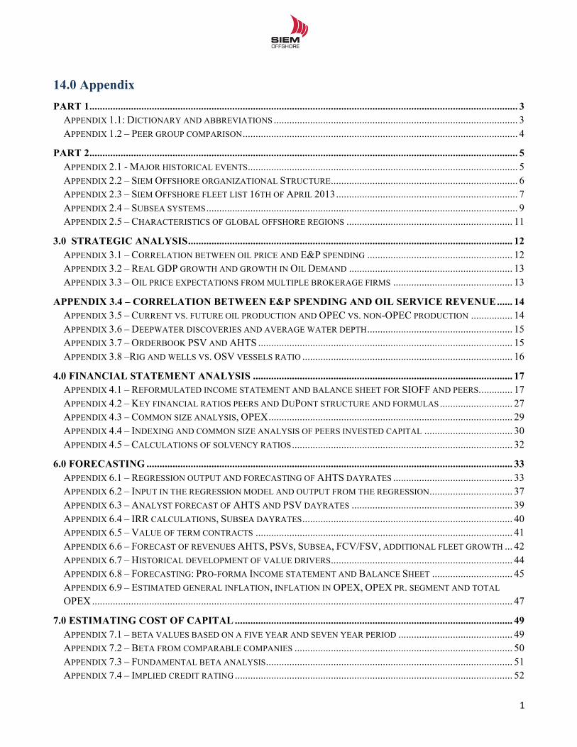
!!
1!!
14.0 Appendix PART 1 ..................................................................................................................................................................... 3
APPENDIX 1.1: DICTIONARY AND ABBREVIATIONS .............................................................................................. 3 APPENDIX 1.2 – PEER GROUP COMPARISON .......................................................................................................... 4
PART 2 ..................................................................................................................................................................... 5 APPENDIX 2.1 - MAJOR HISTORICAL EVENTS ........................................................................................................ 5 APPENDIX 2.2 – SIEM OFFSHORE ORGANIZATIONAL STRUCTURE ........................................................................ 6 APPENDIX 2.3 – SIEM OFFSHORE FLEET LIST 16TH OF APRIL 2013 ...................................................................... 7 APPENDIX 2.4 – SUBSEA SYSTEMS ........................................................................................................................ 9 APPENDIX 2.5 – CHARACTERISTICS OF GLOBAL OFFSHORE REGIONS ................................................................ 11
3.0 STRATEGIC ANALYSIS ............................................................................................................................. 12 APPENDIX 3.1 – CORRELATION BETWEEN OIL PRICE AND E&P SPENDING ........................................................ 12 APPENDIX 3.2 – REAL GDP GROWTH AND GROWTH IN OIL DEMAND ............................................................... 13 APPENDIX 3.3 – OIL PRICE EXPECTATIONS FROM MULTIPLE BROKERAGE FIRMS .............................................. 13
APPENDIX 3.4 – CORRELATION BETWEEN E&P SPENDING AND OIL SERVICE REVENUE ...... 14 APPENDIX 3.5 – CURRENT VS. FUTURE OIL PRODUCTION AND OPEC VS. NON-OPEC PRODUCTION ................ 14 APPENDIX 3.6 – DEEPWATER DISCOVERIES AND AVERAGE WATER DEPTH ........................................................ 15 APPENDIX 3.7 – ORDERBOOK PSV AND AHTS .................................................................................................. 15 APPENDIX 3.8 –RIG AND WELLS VS. OSV VESSELS RATIO ................................................................................. 16
4.0 FINANCIAL STATEMENT ANALYSIS .................................................................................................... 17 APPENDIX 4.1 – REFORMULATED INCOME STATEMENT AND BALANCE SHEET FOR SIOFF AND PEERS. ............ 17 APPENDIX 4.2 – KEY FINANCIAL RATIOS PEERS AND DUPONT STRUCTURE AND FORMULAS ............................ 27 APPENDIX 4.3 – COMMON SIZE ANALYSIS, OPEX .............................................................................................. 29 APPENDIX 4.4 – INDEXING AND COMMON SIZE ANALYSIS OF PEERS INVESTED CAPITAL .................................. 30 APPENDIX 4.5 – CALCULATIONS OF SOLVENCY RATIOS ..................................................................................... 32
6.0 FORECASTING ............................................................................................................................................. 33 APPENDIX 6.1 – REGRESSION OUTPUT AND FORECASTING OF AHTS DAYRATES .............................................. 33 APPENDIX 6.2 – INPUT IN THE REGRESSION MODEL AND OUTPUT FROM THE REGRESSION ................................ 37 APPENDIX 6.3 – ANALYST FORECAST OF AHTS AND PSV DAYRATES .............................................................. 39 APPENDIX 6.4 – IRR CALCULATIONS, SUBSEA DAYRATES ................................................................................. 40 APPENDIX 6.5 – VALUE OF TERM CONTRACTS ................................................................................................... 41 APPENDIX 6.6 – FORECAST OF REVENUES AHTS, PSVS, SUBSEA, FCV/FSV, ADDITIONAL FLEET GROWTH ... 42 APPENDIX 6.7 – HISTORICAL DEVELOPMENT OF VALUE DRIVERS ...................................................................... 44 APPENDIX 6.8 – FORECASTING: PRO-FORMA INCOME STATEMENT AND BALANCE SHEET ............................... 45 APPENDIX 6.9 – ESTIMATED GENERAL INFLATION, INFLATION IN OPEX, OPEX PR. SEGMENT AND TOTAL OPEX .................................................................................................................................................................. 47
7.0 ESTIMATING COST OF CAPITAL ........................................................................................................... 49 APPENDIX 7.1 – BETA VALUES BASED ON A FIVE YEAR AND SEVEN YEAR PERIOD ............................................ 49 APPENDIX 7.2 – BETA FROM COMPARABLE COMPANIES .................................................................................... 50 APPENDIX 7.3 – FUNDAMENTAL BETA ANALYSIS ............................................................................................... 51 APPENDIX 7.4 – IMPLIED CREDIT RATING ........................................................................................................... 52
!!
2!!
8.0 VALUATION .................................................................................................................................................. 53 APPENDIX 8.1 – VALUATION: EQUITY FORECAST, CAPEX AND COMPLETE CASH FLOW STATEMENT .............. 53 APPENDIX 8.2 – MULTIPLES COMPARISON WITH BLOOMBERG .......................................................................... 53
9.0 SENSITIVITY ANALYSIS ........................................................................................................................... 54 APPENDIX 9.1 – SENSITIVITY ANALYSIS ............................................................................................................. 54 APPENDIX 9.2 – TARGET PRICE CONSENSUS ....................................................................................................... 55
10.0 – SUMMARY OF INTERVIEWS WITH INDUSTRY PROFESSIONALS .......................................... 56 APPENDIX 10.1 ØYVIND HAGEN – ANALYST AT ABG SUNDAL COLLIER (NORWEGIAN INVESTMENT BANK) 56 APPENDIX 10.2 - TERJE THORSEN, VP PROJECT CONTROL ESTIMATING, STATOIL ........................................... 57 APPENDIX 10.3 - SIMEN GRANERØD, CLARKSONS OFFSHORE, LONDON, .......................................................... 58
!
!!
3!!
Part 1
Appendix 1.1: Dictionary and abbreviations
AHTS: Anchor Handling Tug Support Vessel
BBL: Barrel of oil
BHP: Break horse power, measure of engine power
Charterer: Company paying for the OSV services
CSV: Construction Support vessel
DP: Dynamic Positioning. Used to maintain a vessel / unit´s position. Different DP systems, ranging from 1-3, with different specifications.
DWT: Dead-weight Tonnage
E&P: Exploration & Production
FCV: Fast Crew Vessel
FSV: Fast Supply Vessel
IMR: Inspection, Maintenance and Repair
ISV: Installation Support Vessel
Jack-up rig: Drilling vessel with three or more extendable legs which are jacked down to the seabed when a drilling location I sreached.
LOA: Length overall, measured in meters
MRSV: Multipurpose field & Remotely Operating Vehicle (ROV) support vessel
OCV: Offshore Construction Vessel
OSCV: Offshore Subsea Construction Vessel
OSRV: Oil Spill Recovery
OSV: Offshort Supply Vessel
PSV: Platform Supply Vessel
ROV: Remotely Operating Vehicle
UDW: Ultra-Deep Waters
CDA: Cargo Deck Area, measured in m2.
QHSE: Quality, Health, Safety and Environment
!!
4!!
Appendix 1.2 – Peer group comparison Source: Compiled by authors / annual reports and homepages.
The choice of peer group is based on operational and strategic factors, and this table identifies those companies
most applicable for the peer group analysis. The Norwegian OSV companies are similar in operation and
management, and they dominate the world fleet of high-end vessels. It is therefore natural to start the analysis by
looking at all the OSV companies listed at Oslo Stock Exchange. Based on the comparison, the following
companies are identified as peers; Farstad Shipping ASA (www.farstad.no), DOF ASA (www.dof.no), Havila
Shipping ASA (www.havila.no) and Solstad Offshore ASA (www.solstad.no).
Comparison*factor SIOFF Farstad DOF Havila Solstad Eidesvik REM DESSC
Medium and*high*end*PSV
HighAEnd*AHTS
OSCV/Subsea vessels
Other*vessels
Newbuilding Program
Historical CAGR**of*revenues above 10%
North Sea*Vessels
Brazil Vessels
Asian Vessels
West African*Vessels
Gulf of*Mexico*Vessels
Stock Exchange*listed
!!
5!!
Part 2
Appendix 2.1 - Major historical events Source: Compiled by authors / Arctic Securities / Oslo Stock Exchange / SIOFF reports
2005 Siem offshore Inc. is spun off from Subsea 7 Inc. and all shareholders in Subsea 7 receives
shares in Siem Offshore on a 1:1 basis. The established company received ownership of six
PSVs newbuild contracts and 10 small vessels in Brazil. Later the same year Rovde Shipping AS
was acquired, expanding the fleet with 4 additional PSVs.1
2006 One PSV was delivered in Q1, another two in Q4. One PSV contract was sold.
The company placed orders with Kleven Maritime for six AHTS vessel plus six options in
addition to four CSVs. Four of the options wore later exercise. One PSV was bought in the
secondhand market. This marked a start for a significant growth strategy with the aim of
expanding both the fleet and the scope of business. Siem also placed orders for two PSVs. Siem
also acquired 60% of the company Well Intervention Solutions for 40 m, later renamed Siem
WIS.2
2007 Siem orders one large PSV newbuild and acquires another PSV in the second hand market. The
PSV newbuild was later cancelled due to the fact that the yard went bankrupt in 2008. Siem also
exercise the last two AHTS options, and transferred the ownership to a pool with the Singapore
based Singa Star.3 The two ATHS was later cancelled, but the pool was expanded to include all
10 of Siems AHTS.
2008 Another newbuild contract is signed for delivery of a large PSV with a cost of NOK 313m for
Eidesvik yard.
2009 Siem orders two large PSVs at STX Brazil for USD 80m. per vessel, increasing the exposure to
the Brazilian market.
2010 Four of the large ATHS vessels are tendered to Petrobras in Brazil on 4Y + 4Y contracts,
strengthening the Brazilian presence further. Later the same year Siem sold one of the PSVs,
replacing it with a newbuilding contract for a larger PSV.
2011 In 2011 Siem acquired Five Ocean Services, a submarine cable installation, repair and
maintenance company for USD 8m. Siem had worked with the company over several years,
using the converted PSV Siem Carrier. In the same year Siem also announced that the ownership
in the scientific drillship Joides Resolution was increased from 50% to 100% for a USD 22.5m
consideration.4
!!!!!!!!!!!!!!!!!!!!!!!!!!!!!!!!!!!!!!!!!!!!!!!!!!!!!!!!!!!!!1!Siem!Offshore!presentation!(Pareto,!2005)!and!Rovde!Shipping!AS!2!Arctic!Securities!–!Initiation!of!coverage!Siem!Offshore!Inc.!pg.!4!3!Arctic!Securities!–!Initiation!of!coverage!Siem!Offshore!Inc.!pg.!5!4!Siem!Offshore!Annual!report!(2011)!pg.!10!
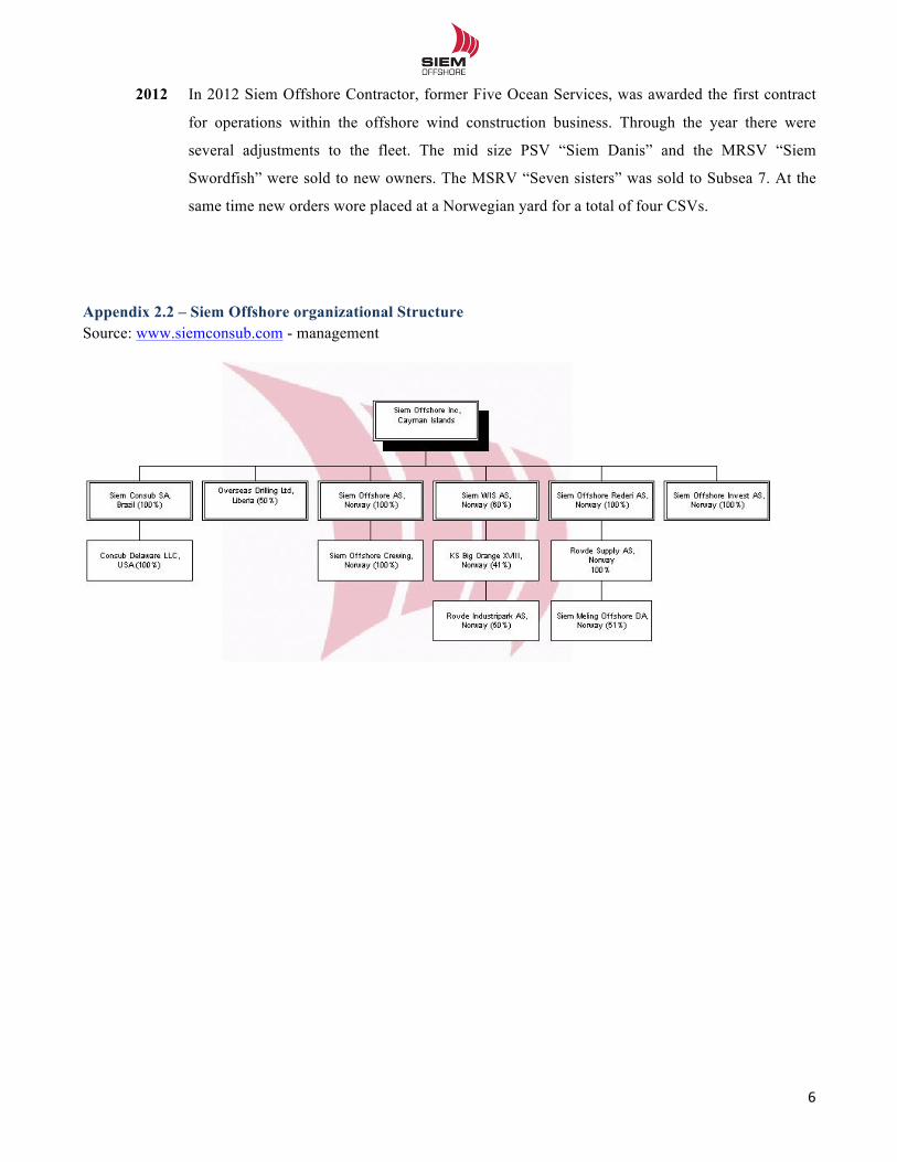
!!
6!!
2012 In 2012 Siem Offshore Contractor, former Five Ocean Services, was awarded the first contract
for operations within the offshore wind construction business. Through the year there were
several adjustments to the fleet. The mid size PSV “Siem Danis” and the MRSV “Siem
Swordfish” were sold to new owners. The MSRV “Seven sisters” was sold to Subsea 7. At the
same time new orders wore placed at a Norwegian yard for a total of four CSVs.
Appendix 2.2 – Siem Offshore organizational Structure Source: www.siemconsub.com - management
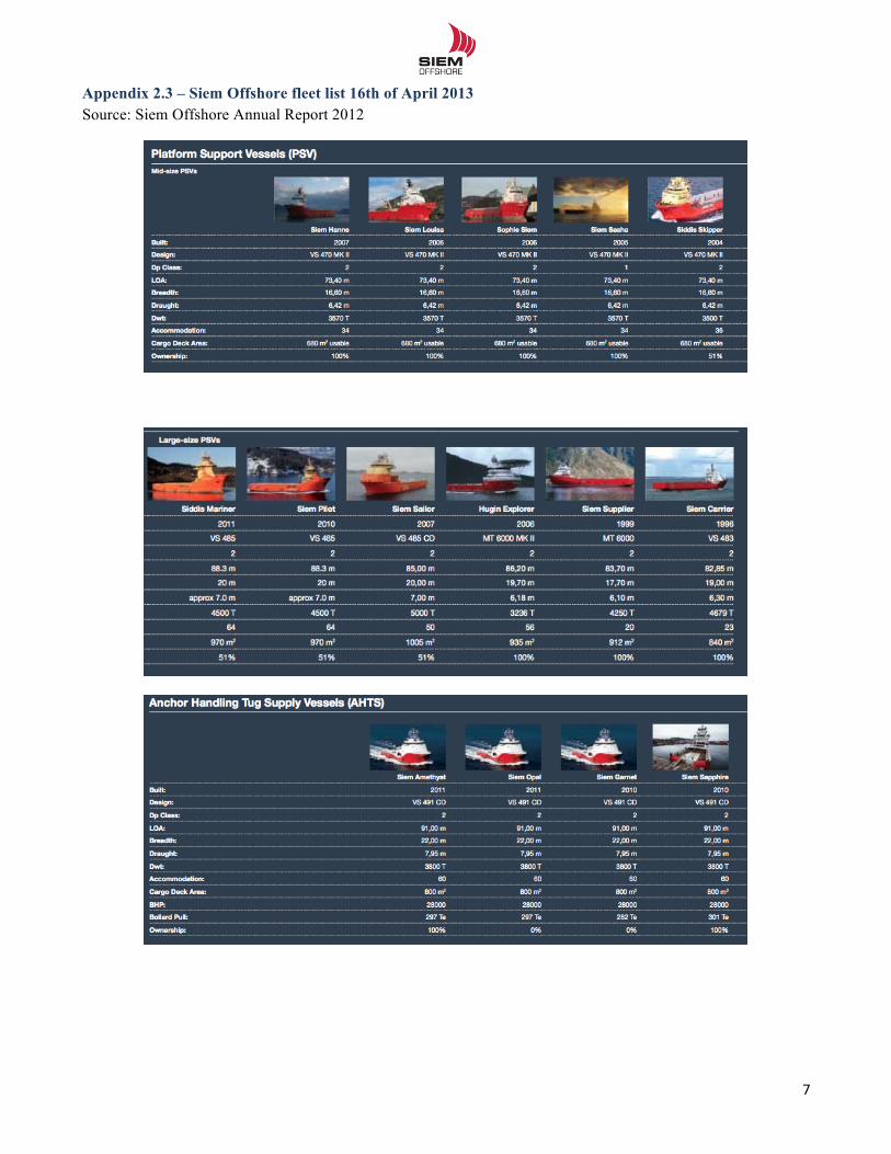
!!
7!!
Appendix 2.3 – Siem Offshore fleet list 16th of April 2013 Source: Siem Offshore Annual Report 2012
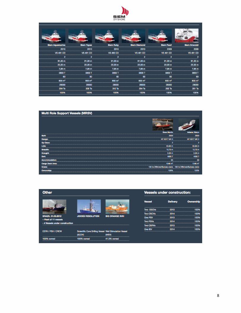
!!
8!!
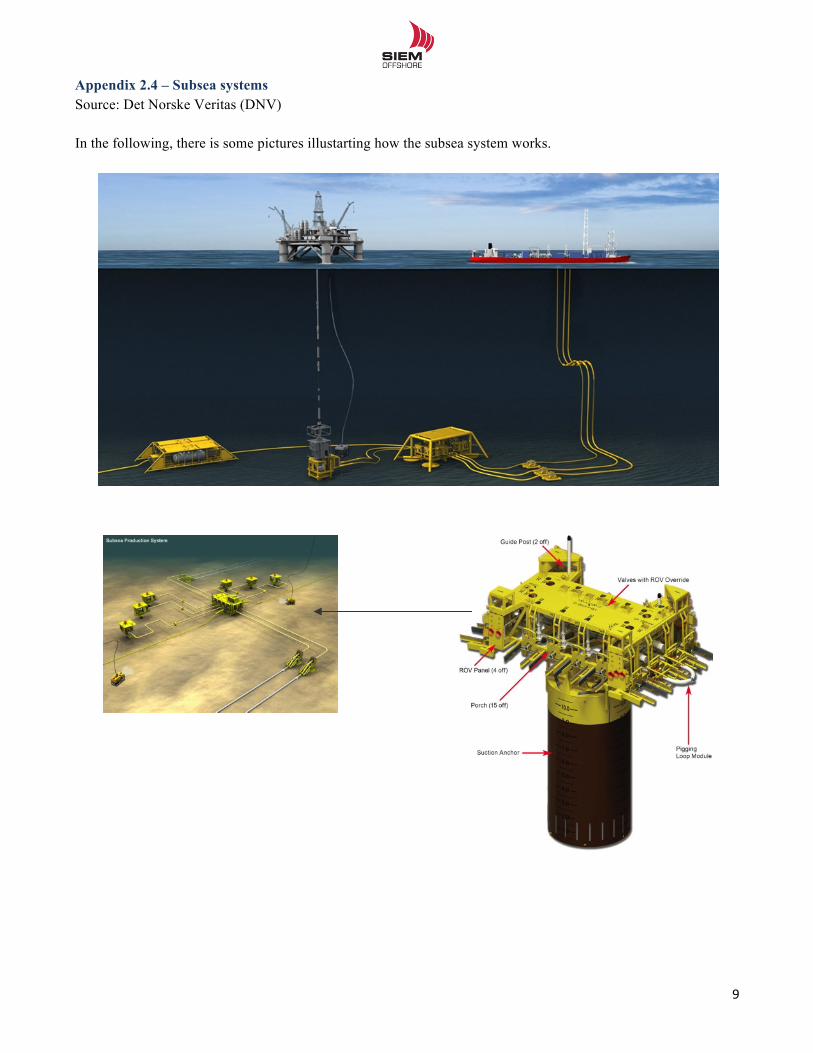
!!
9!!
Appendix 2.4 – Subsea systems Source: Det Norske Veritas (DNV) In the following, there is some pictures illustarting how the subsea system works.
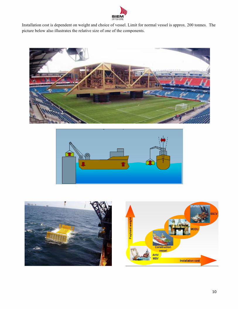
!!
10!!
Installation cost is dependent on weight and choice of vessel. Limit for normal vessel is approx. 200 tonnes. The picture below also illustrates the relative size of one of the components.
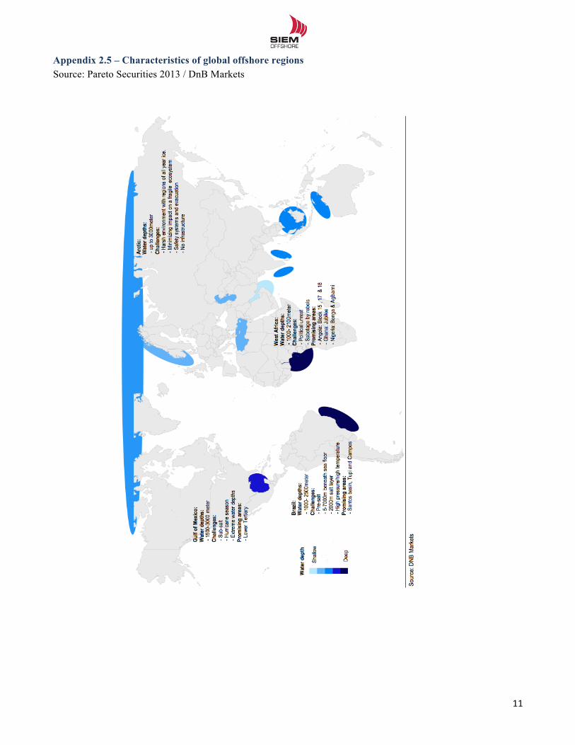
!!
11!!
Appendix 2.5 – Characteristics of global offshore regions Source: Pareto Securities 2013 / DnB Markets
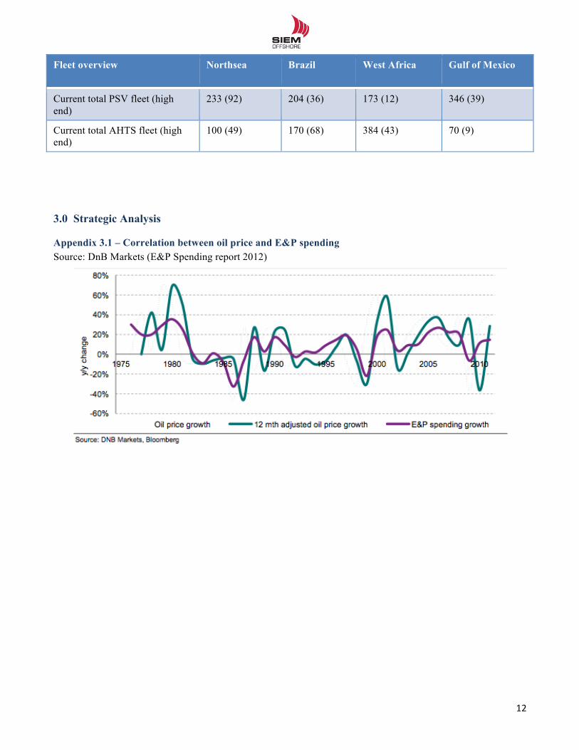
!!
12!!
Fleet overview Northsea Brazil West Africa Gulf of Mexico
Current total PSV fleet (high end)
233 (92) 204 (36) 173 (12) 346 (39)
Current total AHTS fleet (high end)
100 (49) 170 (68) 384 (43) 70 (9)
3.0 Strategic Analysis
Appendix 3.1 – Correlation between oil price and E&P spending Source: DnB Markets (E&P Spending report 2012)
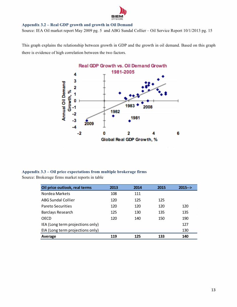
!!
13!!
Appendix 3.2 – Real GDP growth and growth in Oil Demand Source: IEA Oil market report May 2009 pg. 5 and ABG Sundal Collier – Oil Service Report 10/1/2013 pg. 15
This graph explains the relationship between growth in GDP and the growth in oil demand. Based on this graph
there is evidence of high correlation between the two factors.
Appendix 3.3 – Oil price expectations from multiple brokerage firms Source: Brokerage firms market reports in table
Oil$price$outlook,$real$terms 2013 2014 2015 201577>Nordea'Markets 108 111ABG'Sundal'Collier 120 125 125Pareto'Securities 120 120 120 120Barclays'Research 125 130 135 135OECD 120 140 150 190IEA'(Long'term'projections'only) 127EIA'(Long'term'projections'only) 130Average 119 125 133 140
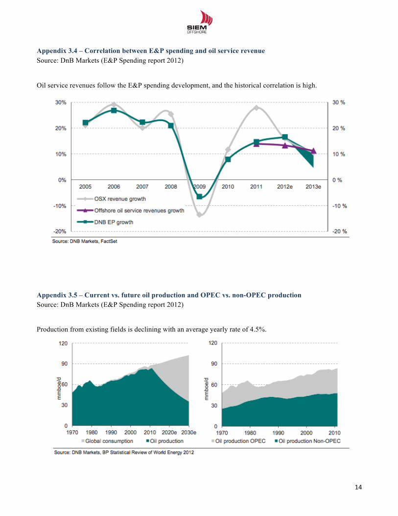
!!
14!!
Appendix 3.4 – Correlation between E&P spending and oil service revenue Source: DnB Markets (E&P Spending report 2012)
Oil service revenues follow the E&P spending development, and the historical correlation is high.
Appendix 3.5 – Current vs. future oil production and OPEC vs. non-OPEC production Source: DnB Markets (E&P Spending report 2012)
Production from existing fields is declining with an average yearly rate of 4.5%.
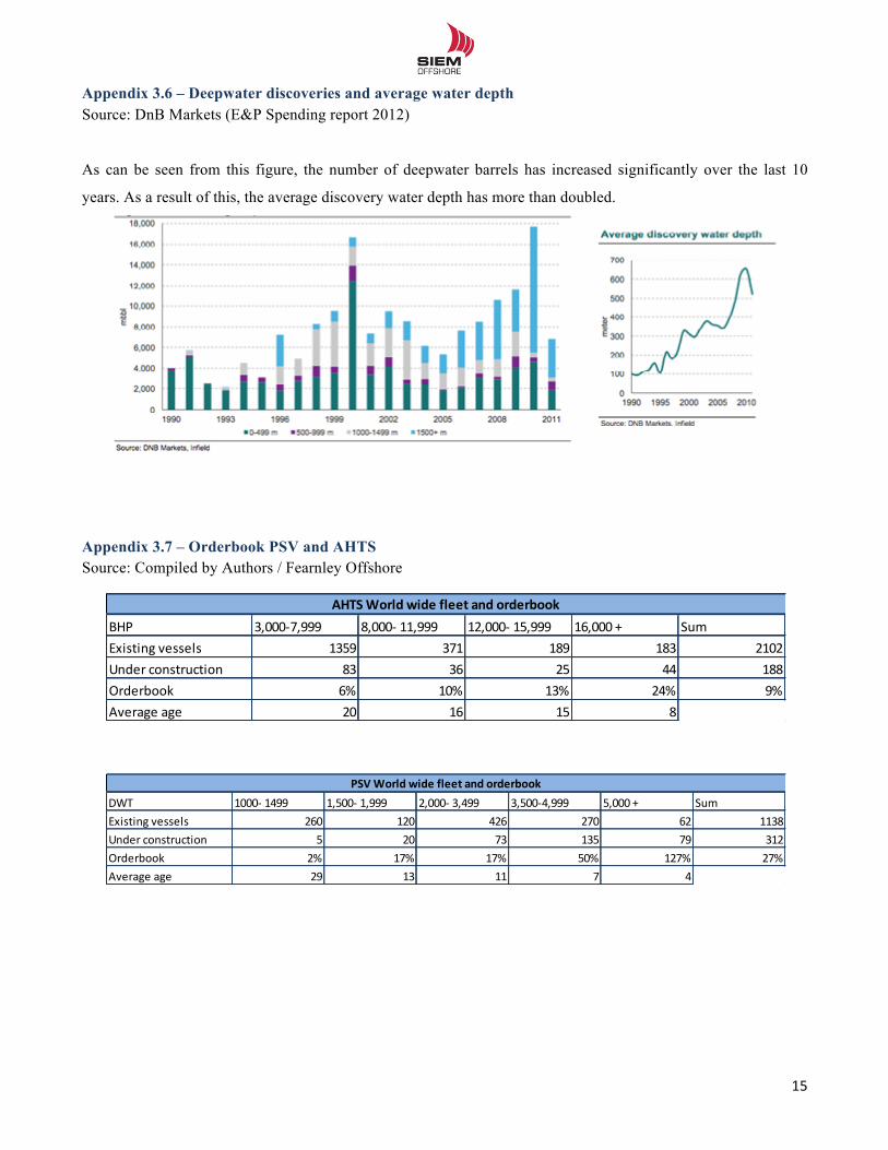
!!
15!!
Appendix 3.6 – Deepwater discoveries and average water depth Source: DnB Markets (E&P Spending report 2012)
As can be seen from this figure, the number of deepwater barrels has increased significantly over the last 10
years. As a result of this, the average discovery water depth has more than doubled.
Appendix 3.7 – Orderbook PSV and AHTS Source: Compiled by Authors / Fearnley Offshore
BHP 3,000'7,999 8,000'+11,999 12,000'+15,999 16,000++ SumExisting+vessels 1359 371 189 183 2102Under+construction 83 36 25 44 188Orderbook 6% 10% 13% 24% 9%Average+age 20 16 15 8
AHTS%World%wide%fleet%and%orderbook
DWT 1000&'1499 1,500&'1,999 2,000&'3,499 3,500&4,999 5,000'+ SumExisting'vessels 260 120 426 270 62 1138Under'construction 5 20 73 135 79 312Orderbook 2% 17% 17% 50% 127% 27%Average'age 29 13 11 7 4
PSV$World$wide$fleet$and$orderbook
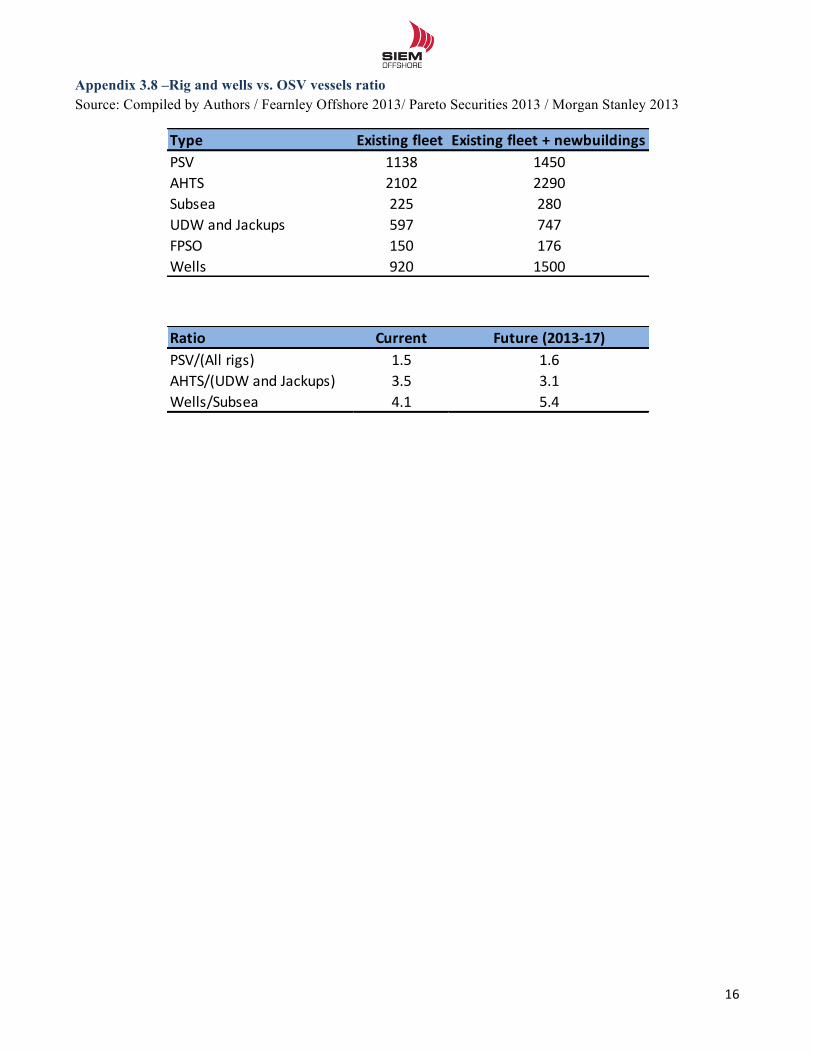
!!
16!!
Appendix 3.8 –Rig and wells vs. OSV vessels ratio Source: Compiled by Authors / Fearnley Offshore 2013/ Pareto Securities 2013 / Morgan Stanley 2013
Type Existing,fleet Existing,fleet,+,newbuildingsPSV 1138 1450AHTS 2102 2290Subsea 225 280UDW7and7Jackups 597 747FPSO 150 176Wells 920 1500
Ratio Current Future,(2013217)PSV/(All(rigs) 1.5 1.6AHTS/(UDW(and(Jackups) 3.5 3.1Wells/Subsea 4.1 5.4
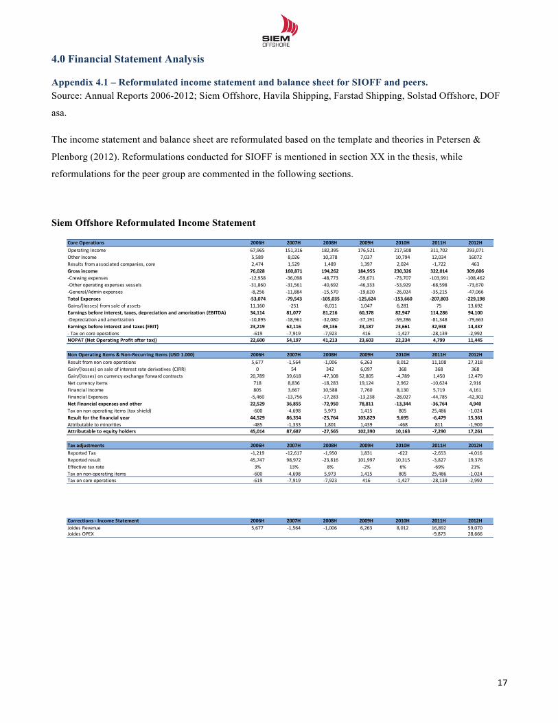
!!
17!!
4.0 Financial Statement Analysis
Appendix 4.1 – Reformulated income statement and balance sheet for SIOFF and peers. Source: Annual Reports 2006-2012; Siem Offshore, Havila Shipping, Farstad Shipping, Solstad Offshore, DOF
asa.
The income statement and balance sheet are reformulated based on the template and theories in Petersen &
Plenborg (2012). Reformulations conducted for SIOFF is mentioned in section XX in the thesis, while
reformulations for the peer group are commented in the following sections.
Siem Offshore Reformulated Income Statement
Core%Operations 2006H 2007H 2008H 2009H 2010H 2011H 2012HOperating*Income 67,965 151,316 182,395 176,521 217,508 311,702 293,071Other*Income 5,589 8,026 10,378 7,037 10,794 12,034 16072Results*from*associated*companies,*core 2,474 1,529 1,489 1,397 2,024 A1,722 463Gross%income 76,028 160,871 194,262 184,955 230,326 322,014 309,606ACrewing*expenses A12,958 A36,098 A48,773 A59,671 A73,707 A103,991 A108,462AOther*operating*expenses*vessels A31,860 A31,561 A40,692 A46,333 A53,929 A68,598 A73,670AGeneral/Admin*expenses A8,256 A11,884 A15,570 A19,620 A26,024 A35,215 A47,066Total%Expenses @53,074 @79,543 @105,035 @125,624 @153,660 @207,803 @229,198Gains/(losses)*from*sale*of*assets 11,160 A251 A8,011 1,047 6,281 75 13,692Earnings%before%interest,%taxes,%depreciation%and%amorization%(EBITDA) 34,114 81,077 81,216 60,378 82,947 114,286 94,100ADepreciation*and*amortization A10,895 A18,961 A32,080 A37,191 A59,286 A81,348 A79,663Earnings%before%interest%and%taxes%(EBIT) 23,219 62,116 49,136 23,187 23,661 32,938 14,437A*Tax*on*core*operations A619 A7,919 A7,923 416 A1,427 A28,139 A2,992NOPAT%(Net%Operating%Profit%after%tax)) 22,600 54,197 41,213 23,603 22,234 4,799 11,445
Non%Operating%Items%&%Non@Recurring%Items%(USD%1.000) 2006H 2007H 2008H 2009H 2010H 2011H 2012HResult*from*non*core*operations 5,677 A1,564 A1,006 6,263 8,012 11,108 27,318Gain/(losses)*on*sale*of*interest*rate*derivatives*(CIRR) 0 54 342 6,097 368 368 368Gain/(losses)*on*currency*exchange*forward*contracts 20,789 39,618 A47,308 52,805 A4,789 1,450 12,479Net*currency*items 718 8,836 A18,283 19,124 2,962 A10,624 2,916Financial*Income 805 3,667 10,588 7,760 8,130 5,719 4,161Financial*Expenses A5,460 A13,756 A17,283 A13,238 A28,027 A44,785 A42,302Net%Financial%expenses%and%other 22,529 36,855 @72,950 78,811 @13,344 @36,764 4,940Tax*on*non*operating*items*(tax*shield) A600 A4,698 5,973 1,415 805 25,486 A1,024Result%for%the%financial%year 44,529 86,354 @25,764 103,829 9,695 @6,479 15,361Attributable*to*minorities A485 A1,333 1,801 1,439 A468 811 A1,900Attributable%to%equity%holders 45,014 87,687 @27,565 102,390 10,163 @7,290 17,261
Tax%adjustments 2006H 2007H 2008H 2009H 2010H 2011H 2012HReported*Tax A1,219 A12,617 A1,950 1,831 A622 A2,653 A4,016Reported*result 45,747 98,972 A23,816 101,997 10,315 A3,827 19,376Effective*tax*rate 3% 13% 8% A2% 6% A69% 21%Tax*on*nonAoperating*items A600 A4,698 5,973 1,415 805 25,486 A1,024Tax*on*core*operations A619 A7,919 A7,923 416 A1,427 A28,139 A2,992
Corrections*+*Income*Statement 2006H 2007H 2008H 2009H 2010H 2011H 2012HJoides'Revenue 5,677 01,564 01,006 6,263 8,012 16,892 59,070Joides'OPEX 09,873 28,666
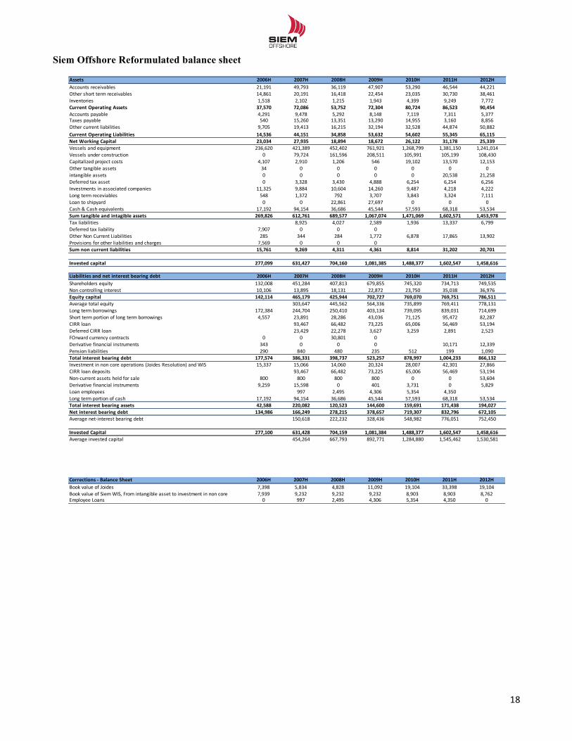
!!
18!!
Siem Offshore Reformulated balance sheet
Assets 2006H 2007H 2008H 2009H 2010H 2011H 2012HAccounts(receivables 21,191 49,793 36,119 47,907 53,290 46,544 44,221Other(short(term(receivables 14,861 20,191 16,418 22,454 23,035 30,730 38,461Inventories 1,518 2,102 1,215 1,943 4,399 9,249 7,772Current1Operating1Assets 37,570 72,086 53,752 72,304 80,724 86,523 90,454Accounts(payable 4,291 9,478 5,292 8,148 7,119 7,311 5,377Taxes(payable 540 15,260 13,351 13,290 14,955 3,160 8,856Other(current(liabilities 9,705 19,413 16,215 32,194 32,528 44,874 50,882Current1Operating1Liabilities 14,536 44,151 34,858 53,632 54,602 55,345 65,115Net1Working1Capital 23,034 27,935 18,894 18,672 26,122 31,178 25,339Vessels(and(equipment 236,620 421,389 452,402 761,921 1,268,799 1,381,150 1,241,014Vessels(under(construction 0 79,724 161,596 208,511 105,991 105,199 108,430Capitalized(project(costs 4,107 2,910 1,206 546 19,102 13,570 12,153Other(tangible(assets 34 0 0 0 0 0 0intangible(assets 0 0 0 0 0 20,538 21,258Deferred(tax(asset 0 3,328 3,430 4,888 6,254 6,254 6,256Investments(in(associated(companies 11,325 9,884 10,604 14,260 9,487 4,218 4,222Long(term(receviables 548 1,372 792 3,707 3,843 3,324 7,111Loan(to(shipyard 0 0 22,861 27,697 0 0 0Cash(&(Cash(equivalents 17,192 94,154 36,686 45,544 57,593 68,318 53,534Sum1tangible1and1intagible1assets 269,826 612,761 689,577 1,067,074 1,471,069 1,602,571 1,453,978Tax(liabilities 8,925 4,027 2,589 1,936 13,337 6,799Deferred(tax(liability 7,907 0 0 0Other(Non(Current(Liabilities 285 344 284 1,772 6,878 17,865 13,902Provisions(for(other(liabilities(and(charges 7,569 0 0 0Sum1non1current1liabilities 15,761 9,269 4,311 4,361 8,814 31,202 20,701
Invested1capital 277,099 631,427 704,160 1,081,385 1,488,377 1,602,547 1,458,616
Liabilities1and1net1interest1bearing1debt 2006H 2007H 2008H 2009H 2010H 2011H 2012HShareholders(equity 132,008 451,284 407,813 679,855 745,320 734,713 749,535Non(controlling(interest 10,106 13,895 18,131 22,872 23,750 35,038 36,976Equity1capital 142,114 465,179 425,944 702,727 769,070 769,751 786,511Average(total(equity 303,647 445,562 564,336 735,899 769,411 778,131Long(term(borrowings 172,384 244,704 250,410 403,134 739,095 839,031 714,699Short(term(portion(of(long(term(borrowings 4,557 23,891 28,286 43,036 71,125 95,472 82,287CIRR(loan 93,467 66,482 73,225 65,006 56,469 53,194Deferred(CIRR(loan 23,429 22,278 3,627 3,259 2,891 2,523FOrward(currency(contracts 0 0 30,801 0Derivative(financial(instruments 343 0 0 0 10,171 12,339Pension(liabilities 290 840 480 235 512 199 1,090Total1interest1bearing1debt 177,574 386,331 398,737 523,257 878,997 1,004,233 866,132Investment(in(non(core(operations((Joides(Resolution)(and(WIS 15,337 15,066 14,060 20,324 28,007 42,301 27,866CIRR(loan(deposits 93,467 66,482 73,225 65,006 56,469 53,194NonXcurrent(assets(held(for(sale 800 800 800 800 0 0 53,604Derivative(financial(instruments 9,259 15,598 0 401 3,731 0 5,829Loan(employees 997 2,495 4,306 5,354 4,350Long(term(portion(of(cash 17,192 94,154 36,686 45,544 57,593 68,318 53,534Total1interest1bearing1assets 42,588 220,082 120,523 144,600 159,691 171,438 194,027Net1interest1bearing1debt 134,986 166,249 278,215 378,657 719,307 832,796 672,105Average(netXinterest(bearing(debt 150,618 222,232 328,436 548,982 776,051 752,450
Invested1Capital 277,100 631,428 704,159 1,081,384 1,488,377 1,602,547 1,458,616Average(invested(capital 454,264 667,793 892,771 1,284,880 1,545,462 1,530,581
Corrections*+*Balance*Sheet 2006H 2007H 2008H 2009H 2010H 2011H 2012HBook$value$of$Joides 7,398 5,834 4,828 11,092 19,104 33,398 19,104Book$value$of$Siem$WIS,$From$intangible$asset$to$investment$in$non$core$ 7,939 9,232 9,232 9,232 8,903 8,903 8,762Employee$Loans 0 997 2,495 4,306 5,354 4,350 0
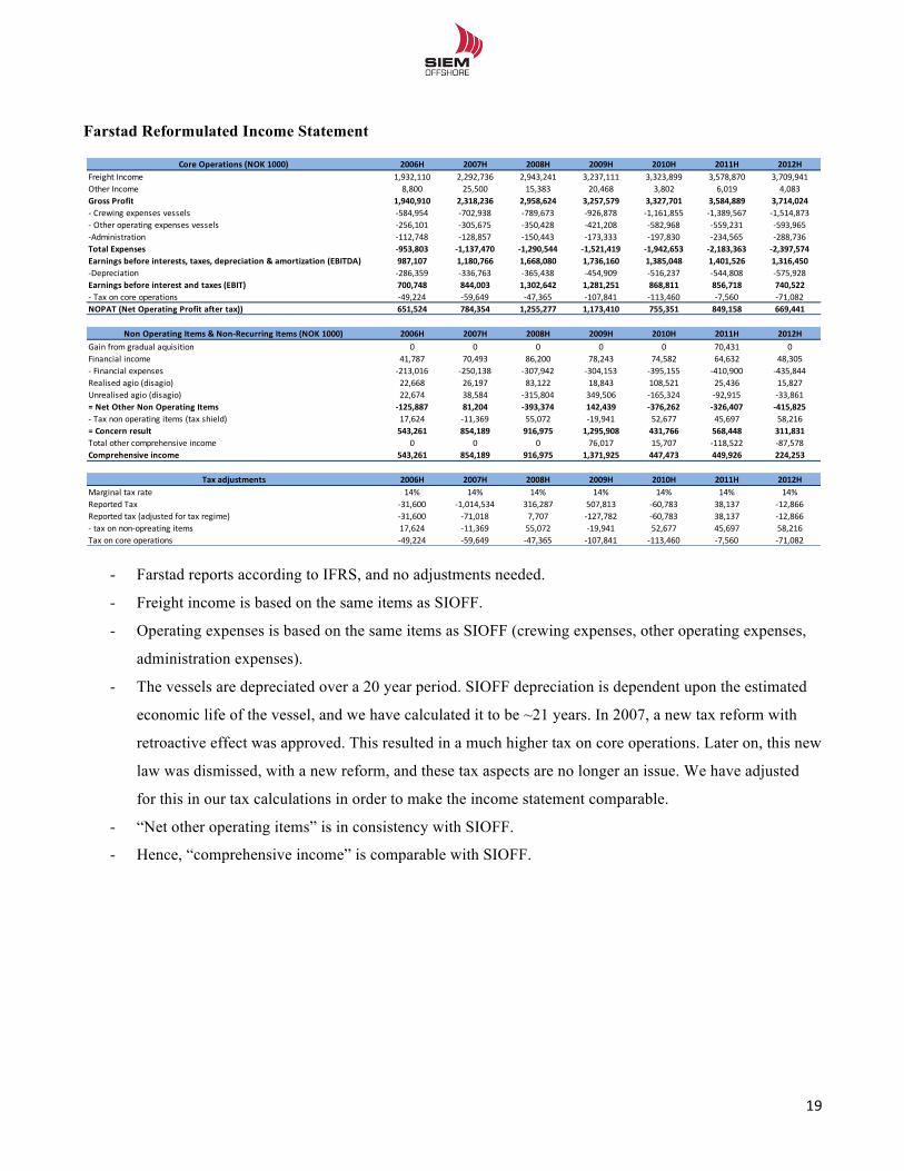
!!
19!!
Farstad Reformulated Income Statement
- Farstad reports according to IFRS, and no adjustments needed.
- Freight income is based on the same items as SIOFF.
- Operating expenses is based on the same items as SIOFF (crewing expenses, other operating expenses,
administration expenses).
- The vessels are depreciated over a 20 year period. SIOFF depreciation is dependent upon the estimated
economic life of the vessel, and we have calculated it to be ~21 years. In 2007, a new tax reform with
retroactive effect was approved. This resulted in a much higher tax on core operations. Later on, this new
law was dismissed, with a new reform, and these tax aspects are no longer an issue. We have adjusted
for this in our tax calculations in order to make the income statement comparable.
- “Net other operating items” is in consistency with SIOFF.
- Hence, “comprehensive income” is comparable with SIOFF.
Core%Operations%(NOK%1000) 2006H 2007H 2008H 2009H 2010H 2011H 2012HFreight(Income 1,932,110 2,292,736 2,943,241 3,237,111 3,323,899 3,578,870 3,709,941Other(Income 8,800 25,500 15,383 20,468 3,802 6,019 4,083Gross%Profit 1,940,910 2,318,236 2,958,624 3,257,579 3,327,701 3,584,889 3,714,024:(Crewing(expenses(vessels :584,954 :702,938 :789,673 :926,878 :1,161,855 :1,389,567 :1,514,873:(Other(operating(expenses(vessels :256,101 :305,675 :350,428 :421,208 :582,968 :559,231 :593,965:Administration :112,748 :128,857 :150,443 :173,333 :197,830 :234,565 :288,736Total%Expenses D953,803 D1,137,470 D1,290,544 D1,521,419 D1,942,653 D2,183,363 D2,397,574Earnings%before%interests,%taxes,%depreciation%&%amortization%(EBITDA) 987,107 1,180,766 1,668,080 1,736,160 1,385,048 1,401,526 1,316,450:Depreciation :286,359 :336,763 :365,438 :454,909 :516,237 :544,808 :575,928Earnings%before%interest%and%taxes%(EBIT) 700,748 844,003 1,302,642 1,281,251 868,811 856,718 740,522:(Tax(on(core(operations :49,224 :59,649 :47,365 :107,841 :113,460 :7,560 :71,082NOPAT%(Net%Operating%Profit%after%tax)) 651,524 784,354 1,255,277 1,173,410 755,351 849,158 669,441
Non%Operating%Items%&%NonDRecurring%Items%(NOK%1000) 2006H 2007H 2008H 2009H 2010H 2011H 2012H
Gain(from(gradual(aquisition 0 0 0 0 0 70,431 0Financial(income 41,787 70,493 86,200 78,243 74,582 64,632 48,305:(Financial(expenses :213,016 :250,138 :307,942 :304,153 :395,155 :410,900 :435,844Realised(agio((disagio) 22,668 26,197 83,122 18,843 108,521 25,436 15,827Unrealised(agio((disagio) 22,674 38,584 :315,804 349,506 :165,324 :92,915 :33,861=%Net%Other%Non%Operating%Items D125,887 81,204 D393,374 142,439 D376,262 D326,407 D415,825:(Tax(non(operating(items((tax(shield) 17,624 :11,369 55,072 :19,941 52,677 45,697 58,216=%Concern%result 543,261 854,189 916,975 1,295,908 431,766 568,448 311,831Total(other(comprehensive(income 0 0 0 76,017 15,707 :118,522 :87,578Comprehensive%income 543,261 854,189 916,975 1,371,925 447,473 449,926 224,253
Tax%adjustments 2006H 2007H 2008H 2009H 2010H 2011H 2012HMarginal(tax(rate 14% 14% 14% 14% 14% 14% 14%Reported(Tax :31,600 :1,014,534 316,287 507,813 :60,783 38,137 :12,866Reported(tax((adjusted(for(tax(regime) :31,600 :71,018 7,707 :127,782 :60,783 38,137 :12,866:(tax(on(non:opreating(items 17,624 :11,369 55,072 :19,941 52,677 45,697 58,216Tax(on(core(operations :49,224 :59,649 :47,365 :107,841 :113,460 :7,560 :71,082
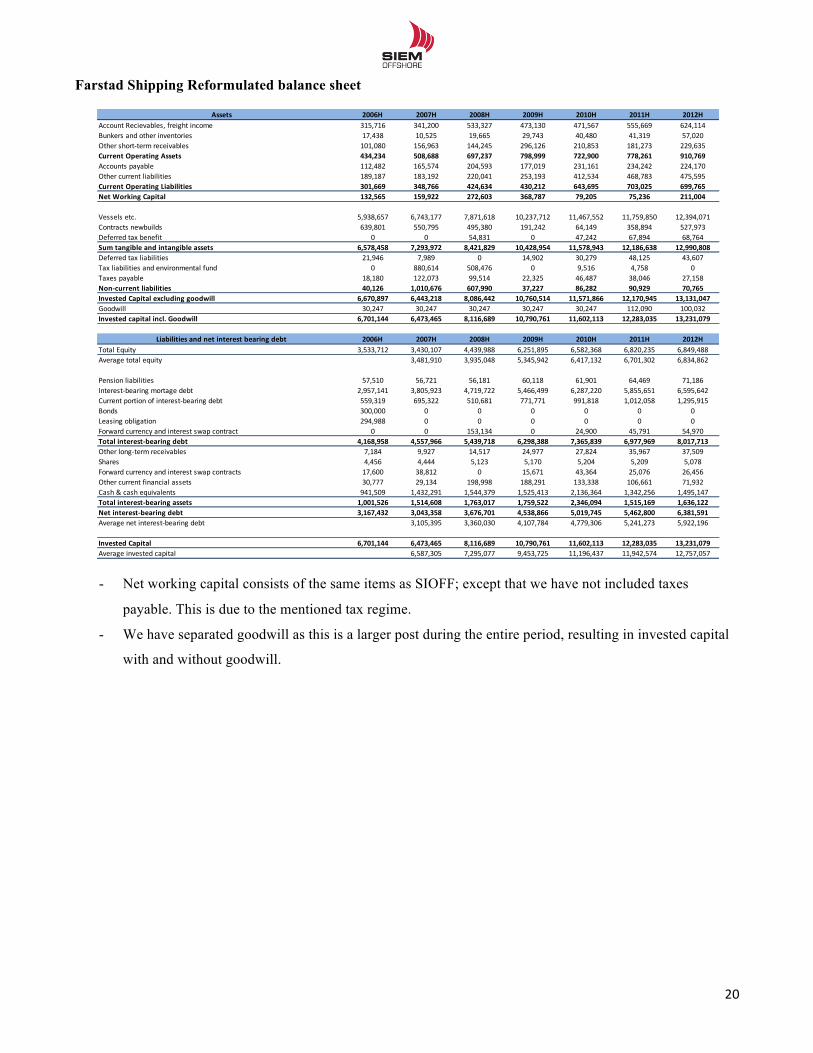
!!
20!!
Farstad Shipping Reformulated balance sheet
- Net working capital consists of the same items as SIOFF; except that we have not included taxes
payable. This is due to the mentioned tax regime.
- We have separated goodwill as this is a larger post during the entire period, resulting in invested capital
with and without goodwill.
Assets 2006H 2007H 2008H 2009H 2010H 2011H 2012HAccount'Recievables,'freight'income 315,716 341,200 533,327 473,130 471,567 555,669 624,114
Bunkers'and'other'inventories 17,438 10,525 19,665 29,743 40,480 41,319 57,020
Other'shortDterm'receivables 101,080 156,963 144,245 296,126 210,853 181,273 229,635
Current1Operating1Assets 434,234 508,688 697,237 798,999 722,900 778,261 910,769Accounts'payable 112,482 165,574 204,593 177,019 231,161 234,242 224,170
Other'current'liabilities 189,187 183,192 220,041 253,193 412,534 468,783 475,595
Current1Operating1Liabilities 301,669 348,766 424,634 430,212 643,695 703,025 699,765Net1Working1Capital1 132,565 159,922 272,603 368,787 79,205 75,236 211,004
Vessels'etc.' 5,938,657 6,743,177 7,871,618 10,237,712 11,467,552 11,759,850 12,394,071
Contracts'newbuilds 639,801 550,795 495,380 191,242 64,149 358,894 527,973
Deferred'tax'benefit' 0 0 54,831 0 47,242 67,894 68,764
Sum1tangible1and1intangible1assets 6,578,458 7,293,972 8,421,829 10,428,954 11,578,943 12,186,638 12,990,808Deferred'tax'liabilities 21,946 7,989 0 14,902 30,279 48,125 43,607
Tax'liabilities'and'environmental'fund 0 880,614 508,476 0 9,516 4,758 0
Taxes'payable 18,180 122,073 99,514 22,325 46,487 38,046 27,158
NonEcurrent1liabilities 40,126 1,010,676 607,990 37,227 86,282 90,929 70,765Invested1Capital1excluding1goodwill 6,670,897 6,443,218 8,086,442 10,760,514 11,571,866 12,170,945 13,131,047Goodwill 30,247 30,247 30,247 30,247 30,247 112,090 100,032
Invested1capital1incl.1Goodwill 6,701,144 6,473,465 8,116,689 10,790,761 11,602,113 12,283,035 13,231,079
Liabilities1and1net1interest1bearing1debt 2006H 2007H 2008H 2009H 2010H 2011H 2012HTotal'Equity 3,533,712 3,430,107 4,439,988 6,251,895 6,582,368 6,820,235 6,849,488
Average'total'equity 3,481,910 3,935,048 5,345,942 6,417,132 6,701,302 6,834,862
Pension'liabilities 57,510 56,721 56,181 60,118 61,901 64,469 71,186
InterestDbearing'mortage'debt 2,957,141 3,805,923 4,719,722 5,466,499 6,287,220 5,855,651 6,595,642
Current'portion'of'interestDbearing'debt 559,319 695,322 510,681 771,771 991,818 1,012,058 1,295,915
Bonds 300,000 0 0 0 0 0 0
Leasing'obligation 294,988 0 0 0 0 0 0
Forward'currency'and'interest'swap'contract 0 0 153,134 0 24,900 45,791 54,970
Total1interestEbearing1debt 4,168,958 4,557,966 5,439,718 6,298,388 7,365,839 6,977,969 8,017,713Other'longDterm'receivables 7,184 9,927 14,517 24,977 27,824 35,967 37,509
Shares 4,456 4,444 5,123 5,170 5,204 5,209 5,078
Forward'currency'and'interest'swap'contracts 17,600 38,812 0 15,671 43,364 25,076 26,456
Other'current'financial'assets 30,777 29,134 198,998 188,291 133,338 106,661 71,932
Cash'&'cash'equivalents 941,509 1,432,291 1,544,379 1,525,413 2,136,364 1,342,256 1,495,147
Total1interestEbearing1assets 1,001,526 1,514,608 1,763,017 1,759,522 2,346,094 1,515,169 1,636,122Net1interestEbearing1debt 3,167,432 3,043,358 3,676,701 4,538,866 5,019,745 5,462,800 6,381,591Average'net'interestDbearing'debt 3,105,395 3,360,030 4,107,784 4,779,306 5,241,273 5,922,196
Invested1Capital1 6,701,144 6,473,465 8,116,689 10,790,761 11,602,113 12,283,035 13,231,079Average'invested'capital' 6,587,305 7,295,077 9,453,725 11,196,437 11,942,574 12,757,057
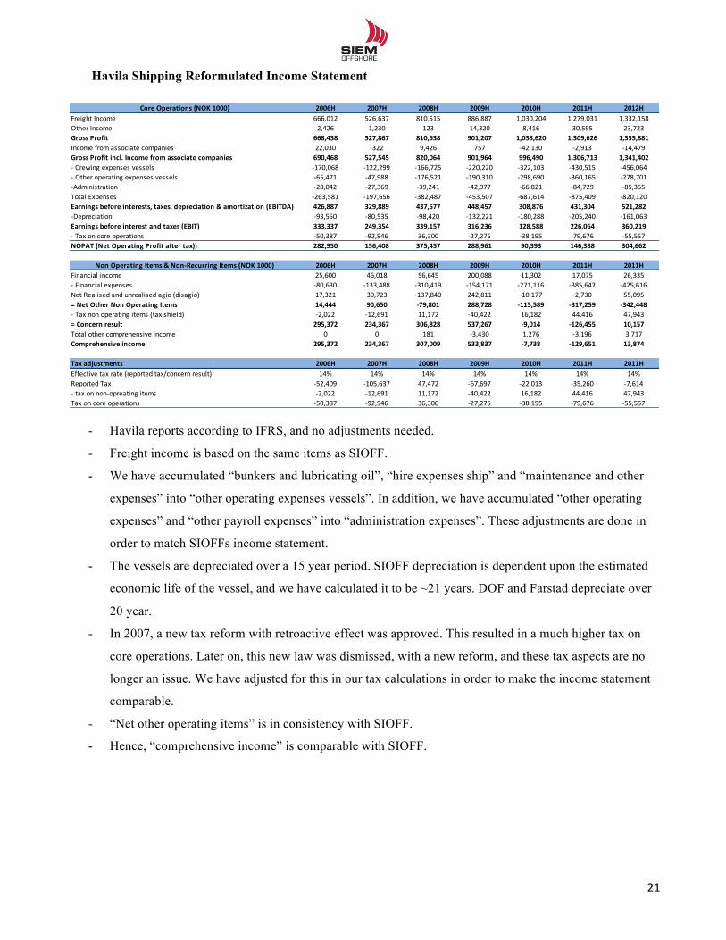
!!
21!!
Havila Shipping Reformulated Income Statement
- Havila reports according to IFRS, and no adjustments needed.
- Freight income is based on the same items as SIOFF.
- We have accumulated “bunkers and lubricating oil”, “hire expenses ship” and “maintenance and other
expenses” into “other operating expenses vessels”. In addition, we have accumulated “other operating
expenses” and “other payroll expenses” into “administration expenses”. These adjustments are done in
order to match SIOFFs income statement.
- The vessels are depreciated over a 15 year period. SIOFF depreciation is dependent upon the estimated
economic life of the vessel, and we have calculated it to be ~21 years. DOF and Farstad depreciate over
20 year.
- In 2007, a new tax reform with retroactive effect was approved. This resulted in a much higher tax on
core operations. Later on, this new law was dismissed, with a new reform, and these tax aspects are no
longer an issue. We have adjusted for this in our tax calculations in order to make the income statement
comparable.
- “Net other operating items” is in consistency with SIOFF.
- Hence, “comprehensive income” is comparable with SIOFF.
Core%Operations%(NOK%1000) 2006H 2007H 2008H 2009H 2010H 2011H 2012HFreight(Income 666,012 526,637 810,515 886,887 1,030,204 1,279,031 1,332,158Other(Income 2,426 1,230 123 14,320 8,416 30,595 23,723Gross%Profit 668,438 527,867 810,638 901,207 1,038,620 1,309,626 1,355,881Income(from(associate(companies 22,030 >322 9,426 757 >42,130 >2,913 >14,479Gross%Profit%incl.%Income%from%associate%companies 690,468 527,545 820,064 901,964 996,490 1,306,713 1,341,402>(Crewing(expenses(vessels >170,068 >122,299 >166,725 >220,220 >322,103 >430,515 >456,064>(Other(operating(expenses(vessels >65,471 >47,988 >176,521 >190,310 >298,690 >360,165 >278,701>Administration >28,042 >27,369 >39,241 >42,977 >66,821 >84,729 >85,355Total(Expenses >263,581 >197,656 >382,487 >453,507 >687,614 >875,409 >820,120Earnings%before%interests,%taxes,%depreciation%&%amortization%(EBITDA) 426,887 329,889 437,577 448,457 308,876 431,304 521,282>Depreciation >93,550 >80,535 >98,420 >132,221 >180,288 >205,240 >161,063Earnings%before%interest%and%taxes%(EBIT) 333,337 249,354 339,157 316,236 128,588 226,064 360,219>(Tax(on(core(operations >50,387 >92,946 36,300 >27,275 >38,195 >79,676 >55,557NOPAT%(Net%Operating%Profit%after%tax)) 282,950 156,408 375,457 288,961 90,393 146,388 304,662
Non%Operating%Items%&%NonPRecurring%Items%(NOK%1000) 2006H 2007H 2008H 2009H 2010H 2011H 2011HFinancial(income 25,600 46,018 56,645 200,088 11,302 17,075 26,335>(Financial(expenses >80,630 >133,488 >310,419 >154,171 >271,116 >385,642 >425,616Net(Realised(and(unrealised(agio((disagio) 17,321 30,723 >137,840 242,811 >10,177 >2,730 55,095=%Net%Other%Non%Operating%Items 14,444 90,650 P79,801 288,728 P115,589 P317,259 P342,448>(Tax(non(operating(items((tax(shield) >2,022 >12,691 11,172 >40,422 16,182 44,416 47,943=%Concern%result 295,372 234,367 306,828 537,267 P9,014 P126,455 10,157Total(other(comprehensive(income 0 0 181 >3,430 1,276 >3,196 3,717Comprehensive%income 295,372 234,367 307,009 533,837 P7,738 P129,651 13,874
Tax%adjustments 2006H 2007H 2008H 2009H 2010H 2011H 2011HEffective(tax(rate((reported(tax/concern(result) 14% 14% 14% 14% 14% 14% 14%Reported(Tax >52,409 >105,637 47,472 >67,697 >22,013 >35,260 >7,614>(tax(on(non>opreating(items >2,022 >12,691 11,172 >40,422 16,182 44,416 47,943Tax(on(core(operations >50,387 >92,946 36,300 >27,275 >38,195 >79,676 >55,557
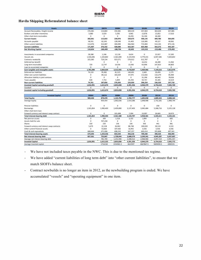
!!
22!!
Havila Shipping Reformulated balance sheet
- We have not included taxes payable in the NWC. This is due to the mentioned tax regime.
- We have added “current liabilities of long term debt” into “other current liabilities”, to ensure that we
match SIOFFs balance sheet.
- Contract newbuilds is no longer an item in 2012, as the newbuilding program is ended. We have
accumulated “vessels” and “operating equipment” in one item.
Assets 2006H 2007H 2008H 2009H 2010H 2011H 2012HAccount'Recievables,'freight'income 276,381 110,804 234,381 309,419 437,063 363,634 347,085Bunkers'and'other'inventories 5,680 5,029 5,595 9,965 13,878 15,852 17,610Other'shortDterm'receivables 0 0 0 10,291 55,194 30,300Current1Assets 282,061 115,833 239,976 329,675 506,135 409,786 364,695Accounts'payable 58,331 62,245 128,590 55,403 110,385 49,127 60,061Other'current'liabilities 113,076 314,087 300,090 366,964 715,083 514,145 875,126Current1Liabilities 171,407 376,332 428,680 422,367 825,468 563,272 935,187Net1Working1Capital1 110,654 A260,499 A188,704 A92,692 A319,333 A153,486 A570,492
Investments'in'associated'companies 28,288 1,246 12,118 9,624 0 22,927 57,392Vessels'etc.' 1,426,696 1,320,802 2,362,690 4,124,935 4,779,231 6,947,585 7,659,842Contracts'newbuilds 325,385 729,234 923,571 570,012 612,787 0Deferred'tax'benefit' 0 0 0 14,252 26,289 11,942LongDterm'receivables 729 12,747 14,556 13,436 63,696 147,815 84,803Loan'to'associated'companies 0 0 0 0 0 0 0Sum1tangible1and1intangible1assets 1,781,098 2,064,029 3,312,935 4,718,007 5,469,966 7,144,616 7,813,979Deferred'tax'liabilities 74,133 95,981 81,515 140,691 2,669 20,493 1,173Other'nonDcurrent'liabilities 0 84,122 183,029 47,975 112,642 110,279 85,900Allocation'liability'in'joint'ventures 0 0 0 0 31,196 60,443 78,026Taxes'payable 628 7,753 5,849 45,293 59,747 45,305 32,619NonAcurrent1liabilities 74,761 187,856 270,393 233,959 206,254 236,520 197,718Invested1Capital1excluding1goodwill 1,816,991 1,615,674 2,853,838 4,391,356 4,944,379 6,754,610 7,045,769Goodwill 0 0 0 0 0 0 0Invested1capital1including1goodwill 1,816,991 1,615,674 2,853,838 4,391,356 4,944,379 6,754,610 7,045,769
Invested1Capital1 2006H 2007H 2008H 2009H 2010H 2011H 2011HTotal1Equity 989,430 879,478 1,125,794 1,702,777 1,695,038 1,809,323 2,008,165Average'Equity 934,454 1,002,636 1,414,286 1,698,908 1,752,181 1,908,744
Pension'liabilities 0 0 0 0 0 230 0Borrowings 1,501,854 1,990,403 2,459,890 3,137,403 3,945,484 5,308,716 5,525,128Other'shortDterm'loanForward'currency'and'interest'swap'contract 0 0 101,698 7,394 13,097 26,665 18,973Total1interestAbearing1debt 1,501,854 1,990,403 2,561,588 3,144,797 3,958,581 5,335,611 5,544,101Net'pension'assets 0 349 1,518 3,102 1,894 0 683Assets'held'for'sale 0 707,230 0 0 0 0 0Shares 150 150 156 156 356 441 381Forward'currency'and'interest'swap'contracts 5,679 22,158 26,062 88,748 100,020 30,519 4,533Other'current'financial'assets 0 53,663 107,565 16,955 3,556 3,556 3,556Cash'&'cash'equivalents 668,464 471,006 698,243 347,257 603,414 355,808 497,341Total1interestAbearing1assets 674,293 1,254,556 833,544 456,218 709,240 390,324 506,494Net1interestAbearing1debt 827,561 735,847 1,728,044 2,688,579 3,249,341 4,945,287 5,037,607Average'net'interestDbearing'debt 781,704 1,231,946 2,208,312 2,968,960 4,097,314 4,991,447Invested1Capital1 1,816,991 1,615,325 2,853,838 4,391,356 4,944,379 6,754,610 7,045,772Average'Invested'capital 1716158 2234581.5 3622597 4667867.5 5849494.5 6900191
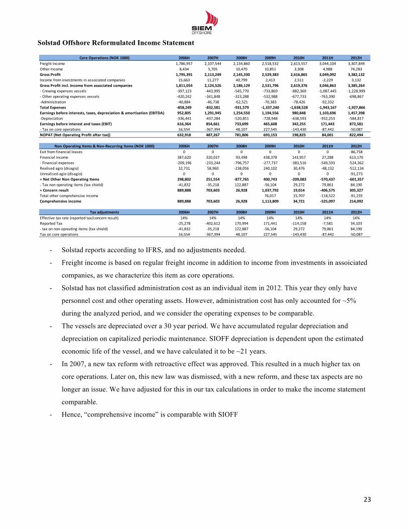
!!
23!!
Solstad Offshore Reformulated Income Statement
- Solstad reports according to IFRS, and no adjustments needed.
- Freight income is based on regular freight income in addition to income from investments in assoiciated
companies, as we characterize this item as core operations.
- Solstad has not classified administration cost as an individual item in 2012. This year they only have
personnel cost and other operating assets. However, administration cost has only accounted for ~5%
during the analyzed period, and we consider the operating expenses to be comparable.
- The vessels are depreciated over a 30 year period. We have accumulated regular depreciation and
depreciation on capitalized periodic maintenance. SIOFF depreciation is dependent upon the estimated
economic life of the vessel, and we have calculated it to be ~21 years.
- In 2007, a new tax reform with retroactive effect was approved. This resulted in a much higher tax on
core operations. Later on, this new law was dismissed, with a new reform, and these tax aspects are no
longer an issue. We have adjusted for this in our tax calculations in order to make the income statement
comparable.
- Hence, “comprehensive income” is comparable with SIOFF
Core%Operations%(NOK%1000) 2006H 2007H 2008H 2009H 2010H 2011H 2012HFreight(Income 1,786,957 2,107,544 2,134,860 2,518,532 2,613,557 3,044,104 3,307,849Other(Income 8,434 5,705 10,470 10,851 3,308 4,988 74,283Gross%Profit 1,795,391 2,113,249 2,145,330 2,529,383 2,616,865 3,049,092 3,382,132Income(from(investments(in(associated(companies 15,663 11,277 40,799 2,413 2,511 @2,229 3,132Gross%Profit%incl.%Income%from%associated%companies 1,811,054 2,124,526 2,186,129 2,531,796 2,619,376 3,046,863 3,385,264@(Crewing(expenses(vessels @397,123 @443,995 @545,770 @733,869 @882,369 @1,087,445 @1,228,999@(Other(operating(expenses(vessels @420,242 @341,848 @323,288 @532,988 @677,733 @763,390 @698,867@Administration @40,884 @46,738 @62,521 @70,383 @78,426 @92,332Total%Expenses I858,249 I832,581 I931,579 I1,337,240 I1,638,528 I1,943,167 I1,927,866Earnings%before%interests,%taxes,%depreciation%&%amortization%(EBITDA) 952,805 1,291,945 1,254,550 1,194,556 980,848 1,103,696 1,457,398@Depreciation @336,441 @437,284 @520,851 @728,948 @638,593 @932,253 @584,817Earnings%before%interest%and%taxes%(EBIT) 616,364 854,661 733,699 465,608 342,255 171,443 872,581@(Tax(on(core(operations 16,554 @367,394 48,107 227,545 @143,430 @87,442 @50,087NOPAT%(Net%Operating%Profit%after%tax)) 632,918 487,267 781,806 693,153 198,825 84,001 822,494
Non%Operating%Items%&%NonIRecurring%Items%(NOK%1000) 2006H 2007H 2008H 2009H 2010H 2011H 2012HExit(from(financial(leases 0 0 0 0 0 0 @86,758Financial(income 387,620 320,037 93,498 438,378 143,957 27,288 613,170@(Financial(expenses @209,196 @233,244 @796,757 @277,737 @383,516 @549,593 @524,362Realised(agio((disagio) 32,731 58,960 @238,056 240,102 30,476 @48,132 @512,134Unrealised(agio((disagio) 0 0 0 0 0 0 @91,273=%Net%Other%Non%Operating%Items 298,802 251,554 I877,765 400,743 I209,083 I570,437 I601,357@(Tax(non(operating(items((tax(shield) @41,832 @35,218 122,887 @56,104 29,272 79,861 84,190=%Concern%result 889,888 703,603 26,928 1,037,792 19,014 I406,575 305,327Total(other(comprehensive(income 76,017 15,707 @118,522 @91,235Comprehensive%income 889,888 703,603 26,928 1,113,809 34,721 I525,097 214,092
Tax%adjustments 2006H 2007H 2008H 2009H 2010H 2011H 2012HEffective(tax(rate((reported(tax/concern(result) 14% 14% 14% 14% 14% 14% 14%Reported(Tax @25,278 @402,612 170,994 171,441 @114,158 @7,581 34,103@(tax(on(non@opreating(items((tax(shield) @41,832 @35,218 122,887 @56,104 29,272 79,861 84,190Tax(on(core(operations 16,554 @367,394 48,107 227,545 @143,430 @87,442 @50,087
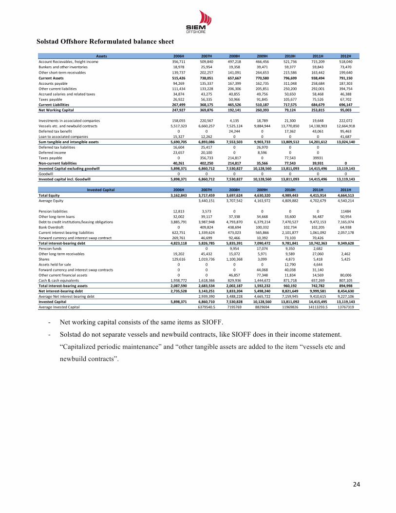
!!
24!!
Solstad Offshore Reformulated balance sheet
- Net working capital consists of the same items as SIOFF.
- Solstad do not separate vessels and newbuild contracts, like SIOFF does in their income statement.
“Capitalized periodic maintenance” and “other tangible assets are added to the item “vessels etc and
newbuild contracts”.
Assets 2006H 2007H 2008H 2009H 2010H 2011H 2012HAccount'Recievables,'freight'income 356,711 509,840 497,218 466,456 521,736 715,209 518,040Bunkers'and'other'inventories 18,978 25,954 19,358 39,471 59,377 59,843 73,470Other'shortDterm'receivables 139,737 202,257 141,091 264,653 215,586 163,442 199,640Current1Assets 515,426 738,051 657,667 770,580 796,699 938,494 791,150Accounts'payable 94,269 135,337 167,399 162,735 311,048 258,684 187,303Other'current'liabilities 111,434 133,228 206,306 205,851 250,200 292,001 394,754Accrued'salaries'and'related'taxes 34,874 43,275 40,855 49,756 50,650 58,468 46,388Taxes'payable 26,922 56,335 50,966 91,845 105,677 75,526 67,702Current1Liabilities 267,499 368,175 465,526 510,187 717,575 684,679 696,147Net1Working1Capital1 247,927 369,876 192,141 260,393 79,124 253,815 95,003
Investments'in'associated'companies 158,055 220,567 4,135 18,789 21,300 19,648 222,072Vessels'etc.'and'newbuild'contracts 5,517,323 6,660,257 7,525,124 9,884,944 13,770,850 14,138,903 12,664,918Deferred'tax'benefit' 0 0 24,244 0 17,362 43,061 95,463Loan'to'associated'companies 15,327 12,262 0 0 0 0 41,687Sum1tangible1and1intangible1assets 5,690,705 6,893,086 7,553,503 9,903,733 13,809,512 14,201,612 13,024,140Deferred'tax'liabilities 16,604 25,417 0 26,970 0 0Deferred'income 23,657 20,100 0 8,596 0 0Taxes'payable 0 356,733 214,817 0 77,543 39931NonDcurrent1liabilities 40,261 402,250 214,817 35,566 77,543 39,931 0Invested1Capital1excluding1goodwill 5,898,371 6,860,712 7,530,827 10,128,560 13,811,093 14,415,496 13,119,143Goodwill 0 0 0 0 0 0 0Invested1capital1incl.1Goodwill 5,898,371 6,860,712 7,530,827 10,128,560 13,811,093 14,415,496 13,119,143
Invested1Capital1 2006H 2007H 2008H 2009H 2010H 2011H 2011HTotal1Equity 3,162,843 3,717,459 3,697,624 4,630,320 4,989,443 4,415,914 4,664,513Average'Equity 3,440,151 3,707,542 4,163,972 4,809,882 4,702,679 4,540,214
Pension'liabilities 12,813 3,573 0 0 0 0 11484Other'longDterm'loans 32,002 39,117 37,338 34,668 33,600 36,487 50,954Debt'to'credit'institutions/leasing'obligations 3,885,791 3,987,948 4,793,870 6,379,214 7,470,527 9,472,153 7,165,074Bank'Overdraft 0 409,824 438,694 100,332 102,734 102,205 64,938Current'interest'bearing'liabilities 622,751 1,339,624 473,023 565,866 2,101,877 1,061,092 2,057,178Forward'currency'and'interest'swap'contract 269,761 46,699 92,466 10,392 73,103 70,426Total1interestDbearing1debt 4,823,118 5,826,785 5,835,391 7,090,472 9,781,841 10,742,363 9,349,628Pension'funds 0 9,954 17,074 9,350 2,682Other'longDterm'receivables 19,202 45,432 15,072 5,971 9,589 27,060 2,462Shares 129,616 1,019,736 1,100,368 3,099 4,873 5,418 5,425Assets'held'for'sale 0 0 0 0 12,790 4,644Forward'currency'and'interest'swap'contracts 0 0 0 44,068 40,038 31,140Other'current'financial'assets 0 0 46,857 77,348 11,834 14,569 80,006Cash'&'cash'equivalents 1,938,772 1,618,366 829,936 1,444,672 871,718 657,269 807,105Total1interestDbearing1assets 2,087,590 2,683,534 2,002,187 1,592,232 960,192 742,782 894,998Net1interestDbearing1debt 2,735,528 3,143,251 3,833,204 5,498,240 8,821,649 9,999,581 8,454,630Average'Net'interest'bearing'debt 2,939,390 3,488,228 4,665,722 7,159,945 9,410,615 9,227,106Invested1Capital1 5,898,371 6,860,710 7,530,828 10,128,560 13,811,092 14,415,495 13,119,143Average'Invested'Capital 6379540.5 7195769 8829694 11969826 14113293.5 13767319
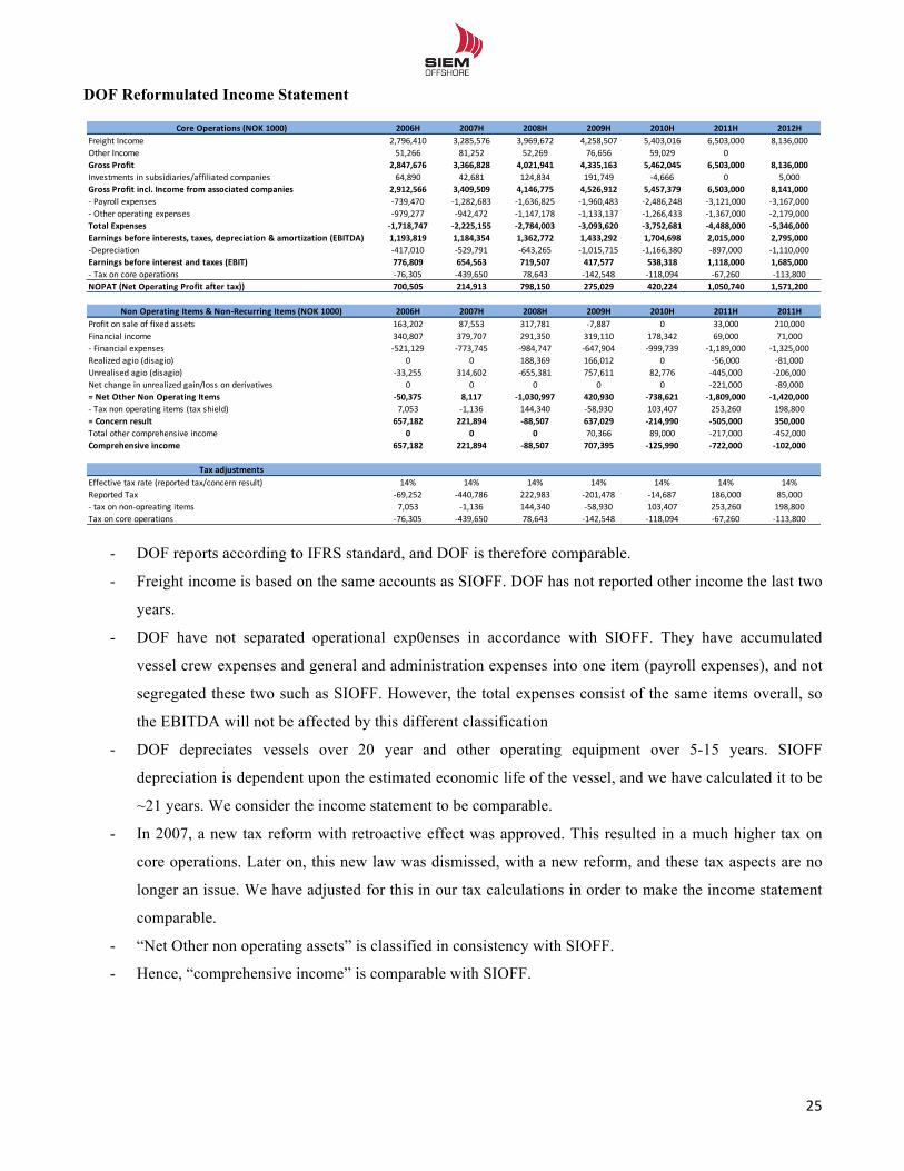
!!
25!!
DOF Reformulated Income Statement
- DOF reports according to IFRS standard, and DOF is therefore comparable.
- Freight income is based on the same accounts as SIOFF. DOF has not reported other income the last two
years.
- DOF have not separated operational exp0enses in accordance with SIOFF. They have accumulated
vessel crew expenses and general and administration expenses into one item (payroll expenses), and not
segregated these two such as SIOFF. However, the total expenses consist of the same items overall, so
the EBITDA will not be affected by this different classification
- DOF depreciates vessels over 20 year and other operating equipment over 5-15 years. SIOFF
depreciation is dependent upon the estimated economic life of the vessel, and we have calculated it to be
~21 years. We consider the income statement to be comparable.
- In 2007, a new tax reform with retroactive effect was approved. This resulted in a much higher tax on
core operations. Later on, this new law was dismissed, with a new reform, and these tax aspects are no
longer an issue. We have adjusted for this in our tax calculations in order to make the income statement
comparable.
- “Net Other non operating assets” is classified in consistency with SIOFF.
- Hence, “comprehensive income” is comparable with SIOFF.
Core%Operations%(NOK%1000) 2006H 2007H 2008H 2009H 2010H 2011H 2012HFreight(Income 2,796,410 3,285,576 3,969,672 4,258,507 5,403,016 6,503,000 8,136,000Other(Income 51,266 81,252 52,269 76,656 59,029 0Gross%Profit 2,847,676 3,366,828 4,021,941 4,335,163 5,462,045 6,503,000 8,136,000Investments(in(subsidiaries/affiliated(companies 64,890 42,681 124,834 191,749 D4,666 0 5,000Gross%Profit%incl.%Income%from%associated%companies 2,912,566 3,409,509 4,146,775 4,526,912 5,457,379 6,503,000 8,141,000D(Payroll(expenses D739,470 D1,282,683 D1,636,825 D1,960,483 D2,486,248 D3,121,000 D3,167,000D(Other(operating(expenses D979,277 D942,472 D1,147,178 D1,133,137 D1,266,433 D1,367,000 D2,179,000Total%Expenses I1,718,747 I2,225,155 I2,784,003 I3,093,620 I3,752,681 I4,488,000 I5,346,000Earnings%before%interests,%taxes,%depreciation%&%amortization%(EBITDA) 1,193,819 1,184,354 1,362,772 1,433,292 1,704,698 2,015,000 2,795,000DDepreciation D417,010 D529,791 D643,265 D1,015,715 D1,166,380 D897,000 D1,110,000Earnings%before%interest%and%taxes%(EBIT) 776,809 654,563 719,507 417,577 538,318 1,118,000 1,685,000D(Tax(on(core(operations D76,305 D439,650 78,643 D142,548 D118,094 D67,260 D113,800NOPAT%(Net%Operating%Profit%after%tax)) 700,505 214,913 798,150 275,029 420,224 1,050,740 1,571,200
Non%Operating%Items%&%NonIRecurring%Items%(NOK%1000) 2006H 2007H 2008H 2009H 2010H 2011H 2011HProfit(on(sale(of(fixed(assets 163,202 87,553 317,781 D7,887 0 33,000 210,000Financial(income 340,807 379,707 291,350 319,110 178,342 69,000 71,000D(Financial(expenses D521,129 D773,745 D984,747 D647,904 D999,739 D1,189,000 D1,325,000Realized(agio((disagio) 0 0 188,369 166,012 0 D56,000 D81,000Unrealised(agio((disagio) D33,255 314,602 D655,381 757,611 82,776 D445,000 D206,000Net(change(in(unrealized(gain/loss(on(derivatives 0 0 0 0 0 D221,000 D89,000=%Net%Other%Non%Operating%Items I50,375 8,117 I1,030,997 420,930 I738,621 I1,809,000 I1,420,000D(Tax(non(operating(items((tax(shield) 7,053 D1,136 144,340 D58,930 103,407 253,260 198,800=%Concern%result 657,182 221,894 I88,507 637,029 I214,990 I505,000 350,000Total(other(comprehensive(income 0 0 0 70,366 89,000 D217,000 D452,000Comprehensive%income 657,182 221,894 I88,507 707,395 I125,990 I722,000 I102,000
Tax%adjustmentsEffective(tax(rate((reported(tax/concern(result) 14% 14% 14% 14% 14% 14% 14%Reported(Tax D69,252 D440,786 222,983 D201,478 D14,687 186,000 85,000D(tax(on(nonDopreating(items 7,053 D1,136 144,340 D58,930 103,407 253,260 198,800Tax(on(core(operations D76,305 D439,650 78,643 D142,548 D118,094 D67,260 D113,800
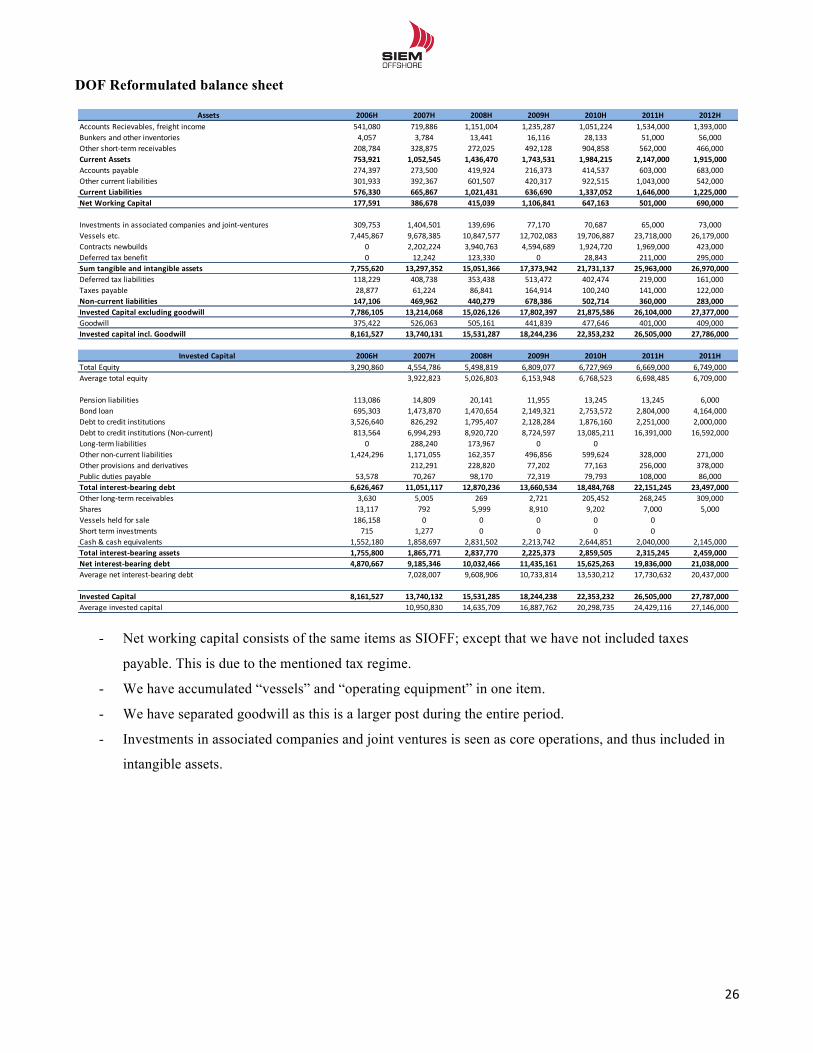
!!
26!!
DOF Reformulated balance sheet
- Net working capital consists of the same items as SIOFF; except that we have not included taxes
payable. This is due to the mentioned tax regime.
- We have accumulated “vessels” and “operating equipment” in one item.
- We have separated goodwill as this is a larger post during the entire period.
- Investments in associated companies and joint ventures is seen as core operations, and thus included in
intangible assets.
Assets 2006H 2007H 2008H 2009H 2010H 2011H 2012HAccounts(Recievables,(freight(income 541,080 719,886 1,151,004 1,235,287 1,051,224 1,534,000 1,393,000Bunkers(and(other(inventories 4,057 3,784 13,441 16,116 28,133 51,000 56,000Other(shortDterm(receivables 208,784 328,875 272,025 492,128 904,858 562,000 466,000Current1Assets 753,921 1,052,545 1,436,470 1,743,531 1,984,215 2,147,000 1,915,000Accounts(payable 274,397 273,500 419,924 216,373 414,537 603,000 683,000Other(current(liabilities 301,933 392,367 601,507 420,317 922,515 1,043,000 542,000Current1Liabilities 576,330 665,867 1,021,431 636,690 1,337,052 1,646,000 1,225,000Net1Working1Capital1 177,591 386,678 415,039 1,106,841 647,163 501,000 690,000
Investments(in(associated(companies(and(jointDventures 309,753 1,404,501 139,696 77,170 70,687 65,000 73,000Vessels(etc.( 7,445,867 9,678,385 10,847,577 12,702,083 19,706,887 23,718,000 26,179,000Contracts(newbuilds 0 2,202,224 3,940,763 4,594,689 1,924,720 1,969,000 423,000Deferred(tax(benefit( 0 12,242 123,330 0 28,843 211,000 295,000Sum1tangible1and1intangible1assets 7,755,620 13,297,352 15,051,366 17,373,942 21,731,137 25,963,000 26,970,000Deferred(tax(liabilities 118,229 408,738 353,438 513,472 402,474 219,000 161,000Taxes(payable 28,877 61,224 86,841 164,914 100,240 141,000 122,000NonDcurrent1liabilities 147,106 469,962 440,279 678,386 502,714 360,000 283,000Invested1Capital1excluding1goodwill 7,786,105 13,214,068 15,026,126 17,802,397 21,875,586 26,104,000 27,377,000Goodwill 375,422 526,063 505,161 441,839 477,646 401,000 409,000Invested1capital1incl.1Goodwill 8,161,527 13,740,131 15,531,287 18,244,236 22,353,232 26,505,000 27,786,000
Invested1Capital1 2006H 2007H 2008H 2009H 2010H 2011H 2011HTotal(Equity 3,290,860 4,554,786 5,498,819 6,809,077 6,727,969 6,669,000 6,749,000Average(total(equity 3,922,823 5,026,803 6,153,948 6,768,523 6,698,485 6,709,000
Pension(liabilities 113,086 14,809 20,141 11,955 13,245 13,245 6,000Bond(loan 695,303 1,473,870 1,470,654 2,149,321 2,753,572 2,804,000 4,164,000Debt(to(credit(institutions 3,526,640 826,292 1,795,407 2,128,284 1,876,160 2,251,000 2,000,000Debt(to(credit(institutions((NonDcurrent) 813,564 6,994,293 8,920,720 8,724,597 13,085,211 16,391,000 16,592,000LongDterm(liabilities 0 288,240 173,967 0 0Other(nonDcurrent(liabilities 1,424,296 1,171,055 162,357 496,856 599,624 328,000 271,000Other(provisions(and(derivatives 212,291 228,820 77,202 77,163 256,000 378,000Public(duties(payable 53,578 70,267 98,170 72,319 79,793 108,000 86,000Total1interestDbearing1debt 6,626,467 11,051,117 12,870,236 13,660,534 18,484,768 22,151,245 23,497,000Other(longDterm(receivables 3,630 5,005 269 2,721 205,452 268,245 309,000Shares 13,117 792 5,999 8,910 9,202 7,000 5,000Vessels(held(for(sale 186,158 0 0 0 0 0Short(term(investments 715 1,277 0 0 0 0Cash(&(cash(equivalents 1,552,180 1,858,697 2,831,502 2,213,742 2,644,851 2,040,000 2,145,000Total1interestDbearing1assets 1,755,800 1,865,771 2,837,770 2,225,373 2,859,505 2,315,245 2,459,000Net1interestDbearing1debt 4,870,667 9,185,346 10,032,466 11,435,161 15,625,263 19,836,000 21,038,000Average(net(interestDbearing(debt 7,028,007 9,608,906 10,733,814 13,530,212 17,730,632 20,437,000
Invested1Capital1 8,161,527 13,740,132 15,531,285 18,244,238 22,353,232 26,505,000 27,787,000Average(invested(capital( 10,950,830 14,635,709 16,887,762 20,298,735 24,429,116 27,146,000
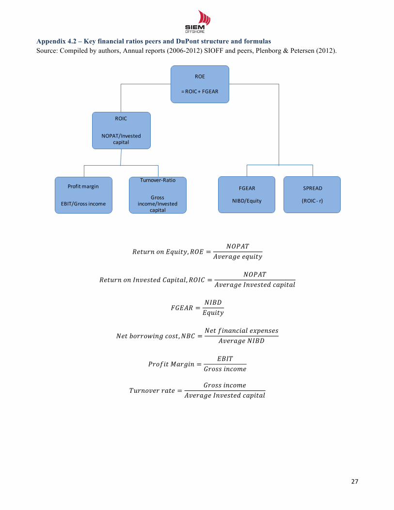
!!
27!!
Appendix 4.2 – Key financial ratios peers and DuPont structure and formulas Source: Compiled by authors, Annual reports (2006-2012) SIOFF and peers, Plenborg & Petersen (2012).
!"#$%&!!"!!"#$%&,!"# = !"#$%!"#$%&#!!"#$%&
!"#$%&!!"!!"#$%&$'!!"#$%"&,!"#$ = !"#$%!"#$%&#!!"#$%&$'!!"#$%"&
!"#$% = !"#$!"#$%&
!"#!!"##"$%&'!!"#$,!"# = !"#!!"#$#%"$&!!"#!$%!%!"#$%&#!!"#$
!"#$%&!!"#$%& = !"#$!"#$$!!"#$%&
!"#$%&'#!!"#$ = !"#$$!!"#$%&!"#$%&#!!"#$%&$'!!"#$%"&
ROE
=%ROIC%+%FGEAR
ROIC
NOPAT/Invested%capital
Profit%margin
EBIT/Gross%income
TurnoverBRatio
Gross%income/Invested%
capital
FGEAR
NIBD/Equity
SPREAD%
(ROIC%B r)
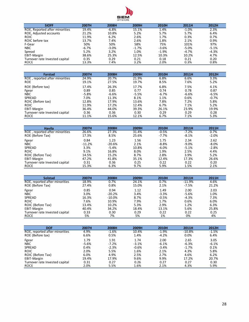
!!
28!!
SIOFF 2007H 2008H 2009H 2010H 2011H 2012HROE,%Reported%after%minorities 19.4% 76.8% 15.1% 1.4% 71.0% 2.3%ROE,%Adjusted%accounts 21.2% 10.8% 5.2% 5.7% 5.7% 6.4%ROIC 11.9% 6.2% 2.6% 1.7% 0.3% 0.7%ROIC%before%tax 13.7% 7.4% 2.6% 1.8% 2.1% 0.9%F7Gear 50% 50% 58% 75% 101% 97%NBC 76.7% 73.0% 71.7% 73.6% 75.0% 75.1%Spread 5.2% 3.2% 1.0% 71.9% 74.7% 74.3%EBIT7Margin 38.6% 25.3% 12.5% 10.3% 10.2% 4.7%Turnover%rate%Invested%capital 0.35 0.29 0.21 0.18 0.21 0.20ROCE 13.3% 7.4% 3.2% 2.0% 0.3% 0.8%
Farstad 2007H 2008H 2009H 2010H 2011H 2012HROE%,%reported%after%minorities 24.9% 20.7% 21.9% 6.8% 6.6% 3.3%ROE 19.1% 27.5% 19.7% 8.5% 7.6% 5.2%ROE%(Before%tax) 17.4% 26.3% 17.7% 6.8% 7.5% 4.1%Fgear 0.89 0.85 0.77 0.74 0.78 0.87NBC 75.8% 76.6% 75.5% 76.7% 76.6% 76.5%SPREAD 7.0% 11.3% 8.1% 1.1% 0.6% 70.7%ROIC%(Before%tax) 12.8% 17.9% 13.6% 7.8% 7.2% 5.8%ROIC 11.9% 17.2% 12.4% 6.7% 7.1% 5.2%EBIT7Margin 36.4% 44.0% 39.3% 26.1% 23.9% 19.9%Turnover%rate%Invested%capital 0.36 0.36 0.30 0.29 0.29 0.28ROCE 11.1% 15.6% 12.1% 6.7% 7.1% 5.3%
Havila 2007H 2008H 2009H 2010H 2011H 2011HROE%,%reported%after%minorities 26.6% 27.3% 31.4% 70.5% 77.2% 0.7%ROE%(Before%Tax) 17.3% 8.5% 25.6% 77.7% 78.1% 72.0%Fgear 0.84 1.23 1.56 1.75 2.34 2.62NBC 711.2% 720.6% 2.1% 78.8% 79.0% 78.0%SPREAD 3.3% 75.4% 10.8% 76.0% 75.1% 72.8%ROIC%% 9.1% 16.8% 8.0% 1.9% 2.5% 4.4%ROIC%(Before%Tax) 14.5% 15.2% 8.7% 2.8% 3.9% 5.2%EBIT7Margin 47.2% 41.8% 35.1% 12.4% 17.3% 26.6%Turnover%rate%Invested%capital 0.31 0.36 0.25 0.22 0.22 0.20ROCE 15.3% 6.3% 9.7% 5.9% 1.5% 2.1%
Solstad 2007H 2008H 2009H 2010H 2011H 2011HROE,%reported%after%minorities 18.9% 0.7% 24.1% 0.7% 711.9% 4.6%ROE%(Before%Tax) 27.4% 0.8% 15.0% 2.1% 77.5% 21.2%Fgear 0.85 0.94 1.12 1.49 2.00 2.03NBC 3.0% 720.2% 3.4% 73.3% 75.6% 1.0%SPREAD 16.3% 710.0% 8.7% 70.5% 74.3% 7.3%ROIC%% 7.6% 10.9% 7.9% 1.7% 0.6% 6.0%ROIC%(Before%Tax) 13.4% 10.2% 5.3% 2.9% 1.2% 6.3%EBIT7Margin 40.4% 34.2% 18.4% 13.1% 5.6% 25.8%Turnover%rate%Invested%capital 0.33 0.30 0.29 0.22 0.22 0.25ROCE 5% 7% 5% 1% 0% 4%
DOF 2007H 2008H 2009H 2010H 2011H 2012HROE,%reported%after%minorities 4.9% 71.6% 10.4% 71.9% 710.8% 71.5%ROE%(Before%tax) 6.6% 0.5% 1.4% 74.2% 0.0% 6.4%Fgear 1.79 1.91 1.74 2.00 2.65 3.05NBC 75.6% 77.2% 73.1% 76.1% 76.3% 76.1%SPREAD 0.4% 72.3% 70.6% 73.4% 71.7% 0.1%ROIC%% 2.0% 5.5% 1.6% 2.1% 4.3% 5.8%ROIC%(Before%Tax) 6.0% 4.9% 2.5% 2.7% 4.6% 6.2%EBIT7Margin 19.4% 17.9% 9.6% 9.9% 17.2% 20.7%Turnover%rate%Invested%capital 0.31 0.27 0.26 0.27 0.27 0.30ROCE 2.0% 5.5% 1.6% 2.1% 4.3% 5.9%
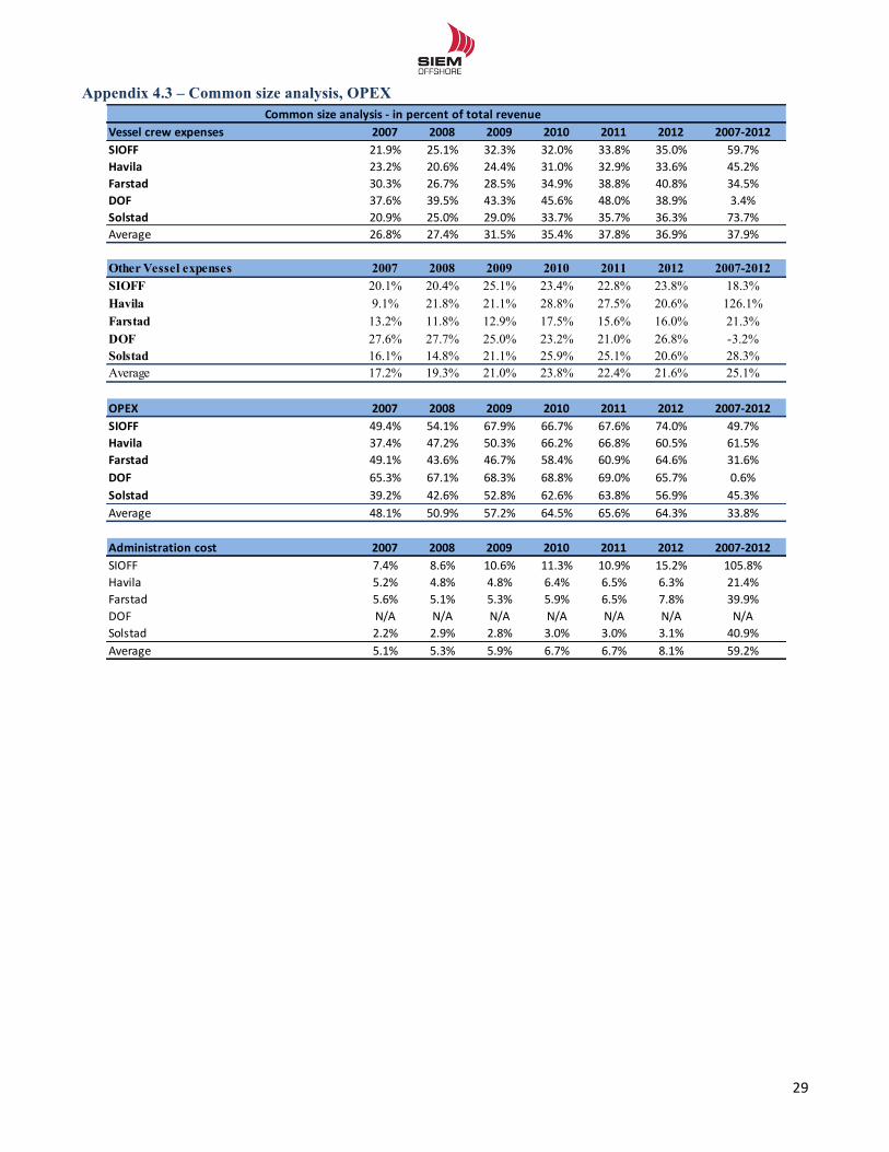
!!
29!!
Appendix 4.3 – Common size analysis, OPEX
Vessel%crew%expenses 2007 2008 2009 2010 2011 2012 200722012SIOFF 21.9% 25.1% 32.3% 32.0% 33.8% 35.0% 59.7%Havila 23.2% 20.6% 24.4% 31.0% 32.9% 33.6% 45.2%Farstad 30.3% 26.7% 28.5% 34.9% 38.8% 40.8% 34.5%DOF 37.6% 39.5% 43.3% 45.6% 48.0% 38.9% 3.4%Solstad 20.9% 25.0% 29.0% 33.7% 35.7% 36.3% 73.7%Average 26.8% 27.4% 31.5% 35.4% 37.8% 36.9% 37.9%
Other Vessel expenses 2007 2008 2009 2010 2011 2012 2007-2012SIOFF 20.1% 20.4% 25.1% 23.4% 22.8% 23.8% 18.3%Havila 9.1% 21.8% 21.1% 28.8% 27.5% 20.6% 126.1%Farstad 13.2% 11.8% 12.9% 17.5% 15.6% 16.0% 21.3%DOF 27.6% 27.7% 25.0% 23.2% 21.0% 26.8% -3.2%Solstad 16.1% 14.8% 21.1% 25.9% 25.1% 20.6% 28.3%Average 17.2% 19.3% 21.0% 23.8% 22.4% 21.6% 25.1%
OPEX 2007 2008 2009 2010 2011 2012 200722012SIOFF 49.4% 54.1% 67.9% 66.7% 67.6% 74.0% 49.7%Havila 37.4% 47.2% 50.3% 66.2% 66.8% 60.5% 61.5%Farstad 49.1% 43.6% 46.7% 58.4% 60.9% 64.6% 31.6%DOF 65.3% 67.1% 68.3% 68.8% 69.0% 65.7% 0.6%Solstad 39.2% 42.6% 52.8% 62.6% 63.8% 56.9% 45.3%Average 48.1% 50.9% 57.2% 64.5% 65.6% 64.3% 33.8%
Administration%cost 2007 2008 2009 2010 2011 2012 200722012SIOFF 7.4% 8.6% 10.6% 11.3% 10.9% 15.2% 105.8%Havila 5.2% 4.8% 4.8% 6.4% 6.5% 6.3% 21.4%Farstad 5.6% 5.1% 5.3% 5.9% 6.5% 7.8% 39.9%DOF N/A N/A N/A N/A N/A N/A N/ASolstad 2.2% 2.9% 2.8% 3.0% 3.0% 3.1% 40.9%Average 5.1% 5.3% 5.9% 6.7% 6.7% 8.1% 59.2%
Common%size%analysis%2%in%percent%of%total%revenue
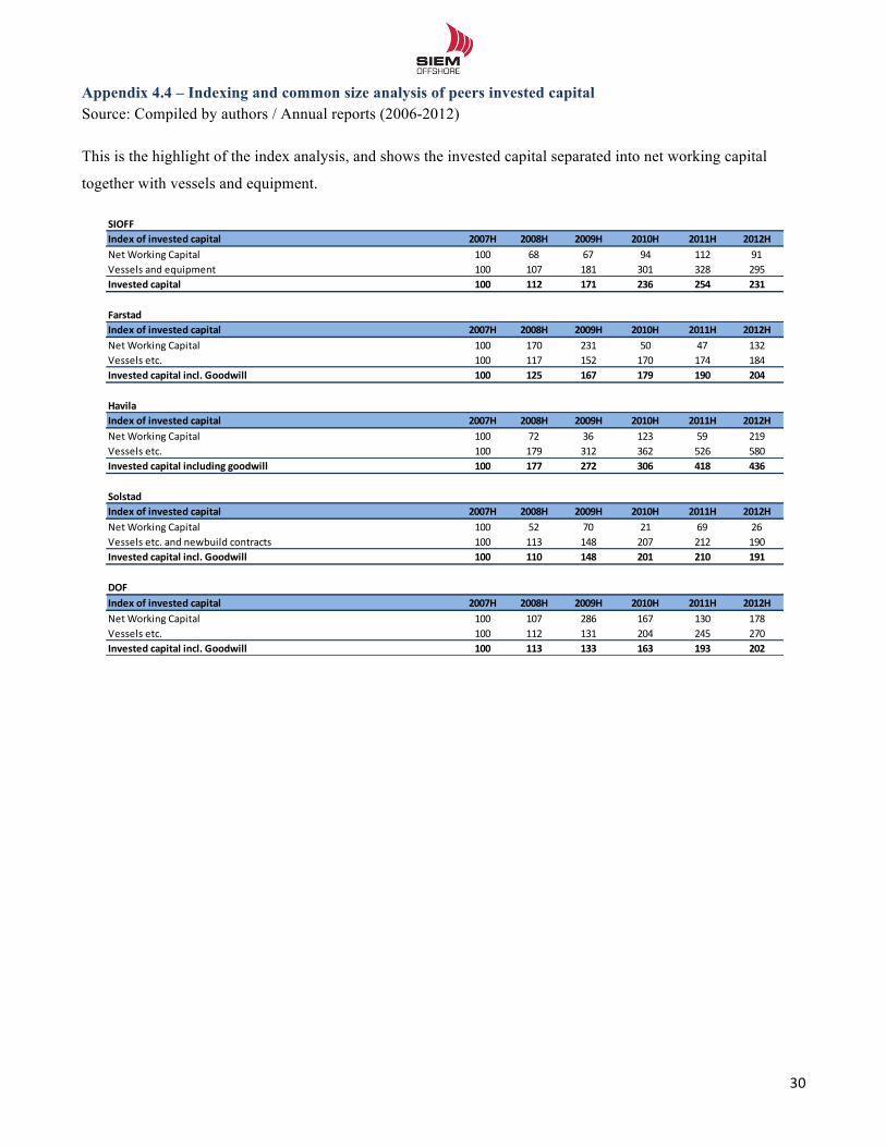
!!
30!!
Appendix 4.4 – Indexing and common size analysis of peers invested capital Source: Compiled by authors / Annual reports (2006-2012)
This is the highlight of the index analysis, and shows the invested capital separated into net working capital
together with vessels and equipment.
SIOFFIndex)of)invested)capital 2007H 2008H 2009H 2010H 2011H 2012HNet$Working$Capital 100 68 67 94 112 91Vessels$and$equipment 100 107 181 301 328 295Invested)capital 100 112 171 236 254 231
FarstadIndex)of)invested)capital 2007H 2008H 2009H 2010H 2011H 2012HNet$Working$Capital$ 100 170 231 50 47 132Vessels$etc.$ 100 117 152 170 174 184Invested)capital)incl.)Goodwill 100 125 167 179 190 204
HavilaIndex)of)invested)capital 2007H 2008H 2009H 2010H 2011H 2012HNet$Working$Capital$ 100 72 36 123 59 219Vessels$etc.$ 100 179 312 362 526 580Invested)capital)including)goodwill 100 177 272 306 418 436
SolstadIndex)of)invested)capital 2007H 2008H 2009H 2010H 2011H 2012HNet$Working$Capital$ 100 52 70 21 69 26Vessels$etc.$and$newbuild$contracts 100 113 148 207 212 190Invested)capital)incl.)Goodwill 100 110 148 201 210 191
DOFIndex)of)invested)capital 2007H 2008H 2009H 2010H 2011H 2012HNet$Working$Capital$ 100 107 286 167 130 178Vessels$etc.$ 100 112 131 204 245 270Invested)capital)incl.)Goodwill 100 113 133 163 193 202
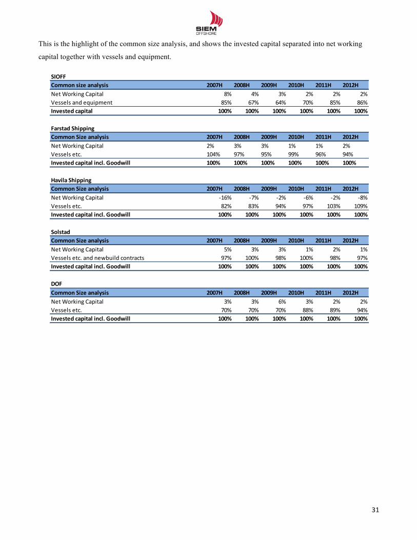
!!
31!!
This is the highlight of the common size analysis, and shows the invested capital separated into net working
capital together with vessels and equipment.
SIOFFCommon)size)analysis) 2007H 2008H 2009H 2010H 2011H 2012HNet$Working$Capital 8% 4% 3% 2% 2% 2%Vessels$and$equipment 85% 67% 64% 70% 85% 86%Invested)capital 100% 100% 100% 100% 100% 100%
Farstad)ShippingCommon)Size)analysis 2007H 2008H 2009H 2010H 2011H 2012HNet$Working$Capital$ 2% 3% 3% 1% 1% 2%Vessels$etc.$ 104% 97% 95% 99% 96% 94%Invested)capital)incl.)Goodwill 100% 100% 100% 100% 100% 100%
Havila)ShippingCommon)Size)analysis 2007H 2008H 2009H 2010H 2011H 2012HNet$Working$Capital$ C16% C7% C2% C6% C2% C8%Vessels$etc.$ 82% 83% 94% 97% 103% 109%Invested)capital)incl.)Goodwill 100% 100% 100% 100% 100% 100%
SolstadCommon)Size)analysis 2007H 2008H 2009H 2010H 2011H 2012HNet$Working$Capital$ 5% 3% 3% 1% 2% 1%Vessels$etc.$and$newbuild$contracts 97% 100% 98% 100% 98% 97%Invested)capital)incl.)Goodwill 100% 100% 100% 100% 100% 100%
DOFCommon)Size)analysis 2007H 2008H 2009H 2010H 2011H 2012HNet$Working$Capital$ 3% 3% 6% 3% 2% 2%Vessels$etc.$ 70% 70% 70% 88% 89% 94%Invested)capital)incl.)Goodwill 100% 100% 100% 100% 100% 100%
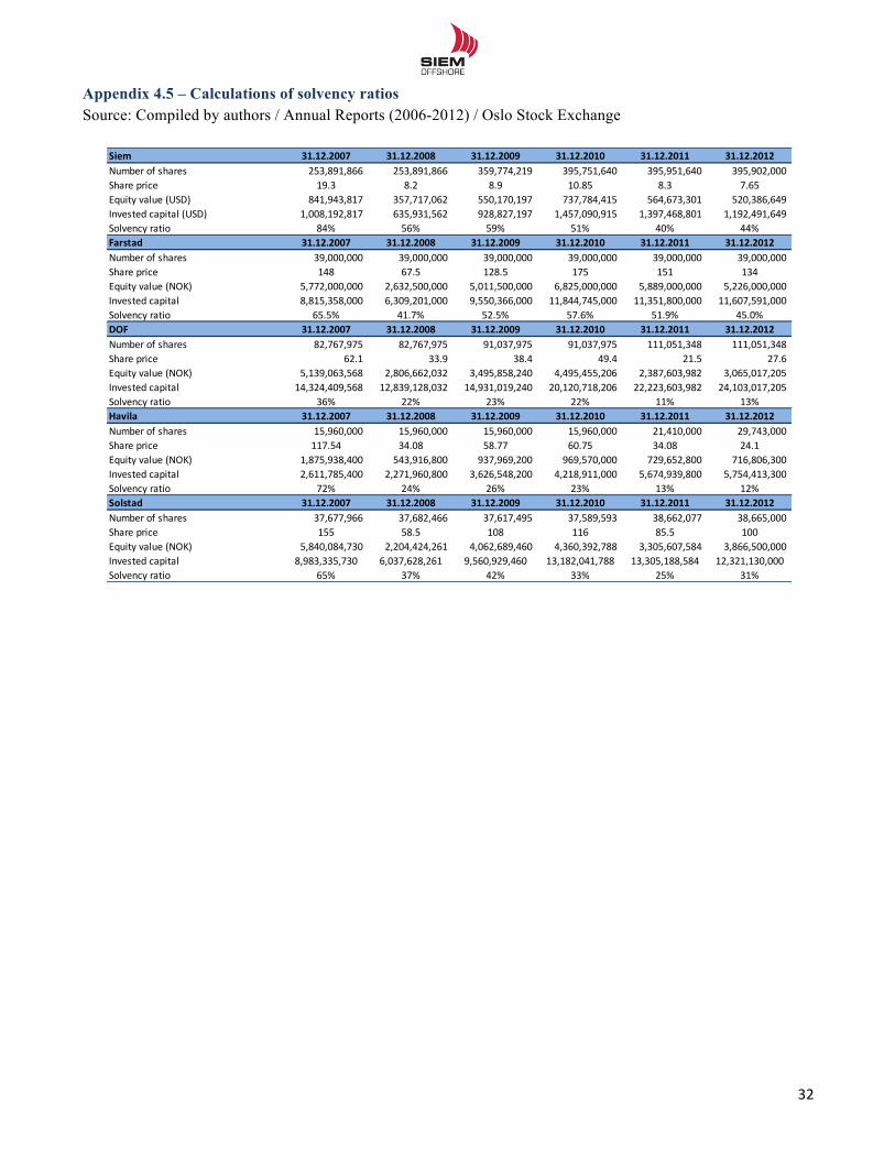
!!
32!!
Appendix 4.5 – Calculations of solvency ratios Source: Compiled by authors / Annual Reports (2006-2012) / Oslo Stock Exchange
Siem 31.12.2007 31.12.2008 31.12.2009 31.12.2010 31.12.2011 31.12.2012Number'of'shares 253,891,866'''''''' 253,891,866'''''''' 359,774,219'''''''' 395,751,640'''''''' 395,951,640'''''''' 395,902,000''''''''Share'price 19.3 8.2 8.9 10.85 8.3 7.65Equity'value'(USD) 841,943,817'''''''' 357,717,062'''''''' 550,170,197'''''''' 737,784,415'''''''' 564,673,301'''''''' 520,386,649''''''''Invested'capital'(USD) 1,008,192,817''''' 635,931,562'''''''' 928,827,197'''''''' 1,457,090,915''''' 1,397,468,801''''' 1,192,491,649'''''Solvency'ratio 84% 56% 59% 51% 40% 44%Farstad 31.12.2007 31.12.2008 31.12.2009 31.12.2010 31.12.2011 31.12.2012Number'of'shares 39,000,000'''''''''' 39,000,000'''''''''' 39,000,000'''''''''' 39,000,000'''''''''' 39,000,000'''''''''' 39,000,000''''''''''Share'price 148 67.5 128.5 175 151 134Equity'value'(NOK) 5,772,000,000''''' 2,632,500,000''''' 5,011,500,000''''' 6,825,000,000''''' 5,889,000,000''''' 5,226,000,000'''''Invested'capital 8,815,358,000''''' 6,309,201,000''''' 9,550,366,000''''' 11,844,745,000''' 11,351,800,000''' 11,607,591,000'''Solvency'ratio 65.5% 41.7% 52.5% 57.6% 51.9% 45.0%DOF 31.12.2007 31.12.2008 31.12.2009 31.12.2010 31.12.2011 31.12.2012Number'of'shares 82,767,975'''''''''' 82,767,975'''''''''' 91,037,975'''''''''' 91,037,975'''''''''' 111,051,348'''''''' 111,051,348''''''''Share'price 62.1''''''''''''''''''''' 33.9''''''''''''''''''''' 38.4''''''''''''''''''''' 49.4''''''''''''''''''''' 21.5''''''''''''''''''''' 27.6'''''''''''''''''''''Equity'value'(NOK) 5,139,063,568''''' 2,806,662,032''''' 3,495,858,240''''' 4,495,455,206''''' 2,387,603,982''''' 3,065,017,205'''''Invested'capital 14,324,409,568''' 12,839,128,032''' 14,931,019,240''' 20,120,718,206''' 22,223,603,982''' 24,103,017,205'''Solvency'ratio 36% 22% 23% 22% 11% 13%Havila 31.12.2007 31.12.2008 31.12.2009 31.12.2010 31.12.2011 31.12.2012Number'of'shares 15,960,000'''''''''' 15,960,000'''''''''' 15,960,000'''''''''' 15,960,000'''''''''' 21,410,000'''''''''' 29,743,000''''''''''Share'price 117.54 34.08 58.77 60.75 34.08 24.1Equity'value'(NOK) 1,875,938,400''''' 543,916,800'''''''' 937,969,200'''''''' 969,570,000'''''''' 729,652,800'''''''' 716,806,300''''''''Invested'capital 2,611,785,400''''' 2,271,960,800''''' 3,626,548,200''''' 4,218,911,000''''' 5,674,939,800''''' 5,754,413,300'''''Solvency'ratio 72% 24% 26% 23% 13% 12%Solstad 31.12.2007 31.12.2008 31.12.2009 31.12.2010 31.12.2011 31.12.2012Number'of'shares 37,677,966'''''''''' 37,682,466'''''''''' 37,617,495'''''''''' 37,589,593'''''''''' 38,662,077'''''''''' 38,665,000''''''''''Share'price 155 58.5 108 116 85.5 100Equity'value'(NOK) 5,840,084,730''''' 2,204,424,261''''' 4,062,689,460''''' 4,360,392,788''''' 3,305,607,584''''' 3,866,500,000'''''Invested'capital 8,983,335,730 6,037,628,261 9,560,929,460 13,182,041,788 13,305,188,584 12,321,130,000Solvency'ratio 65% 37% 42% 33% 25% 31%
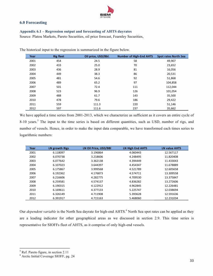
!!
33!!
6.0 Forecasting
Appendix 6.1 – Regression output and forecasting of AHTS dayrates Source: Platou Markets, Pareto Securities, oil price forecast, Fearnley Securities,
The historical input to the regression is summarized in the figure below.
We have applied a time series from 2001-2013, which we characterize as sufficient as it covers an entire cycle of
8-10 years.5 The input to the time series is based on different quantities, such as USD, number of rigs, and
number of vessels. Hence, in order to make the input data comparable, we have transformed each times series to
logarithmic numbers:
Our dependent variable is the North Sea dayrate for high-end AHTS.6 North Sea spot rates can be applied as they
are a leading indicator for other geographical areas as we discussed in section 2.9. This time series is
representative for SIOFFs fleet of AHTS, as it comprise of only high-end vessels.
!!!!!!!!!!!!!!!!!!!!!!!!!!!!!!!!!!!!!!!!!!!!!!!!!!!!!!!!!!!!!5 Ref. Pareto figure, in section 2.11 6 Arctic Initial Coverage SIOFF, pg. 24
Year Rig(fleet Oil(price,(USD/Bbl. Number(of(High=End(AHTS Spot(rates(North(Sea2001 454 24.5 58 49,9072002 433 25.0 70 23,6522003 436 28.9 81 16,0562004 449 38.3 86 20,5312005 481 54.6 92 51,8682006 489 65.2 97 104,8582007 501 72.4 111 112,0442008 523 96.9 126 101,0542009 488 61.7 143 35,5002010 478 79.6 186 29,4222011 559 111.3 220 51,1462012 597 111.6 237 35,662
Year LN'growth'Rigs LN'Oil'Price,'USD/BBl LN'High'End'AHTS LN'value'AHTS2001 6.118097 3.196864 4.060443 12.5671172002 6.070738 3.218606 4.248495 11.8204082003 6.077642 3.362138 4.394449 11.4330432004 6.107023 3.644397 4.454347 11.6788892005 6.175867 3.999568 4.521789 12.6056582006 6.192362 4.176873 4.574711 13.3095582007 6.216606 4.282775 4.709530 13.3758472008 6.259581 4.574137 4.836282 13.2726062009 6.190315 4.122912 4.962845 12.2264812010 6.169611 4.377133 5.225747 12.0386942011 6.326149 4.711908 5.393628 12.5916362012 6.391917 4.715163 5.468060 12.231034
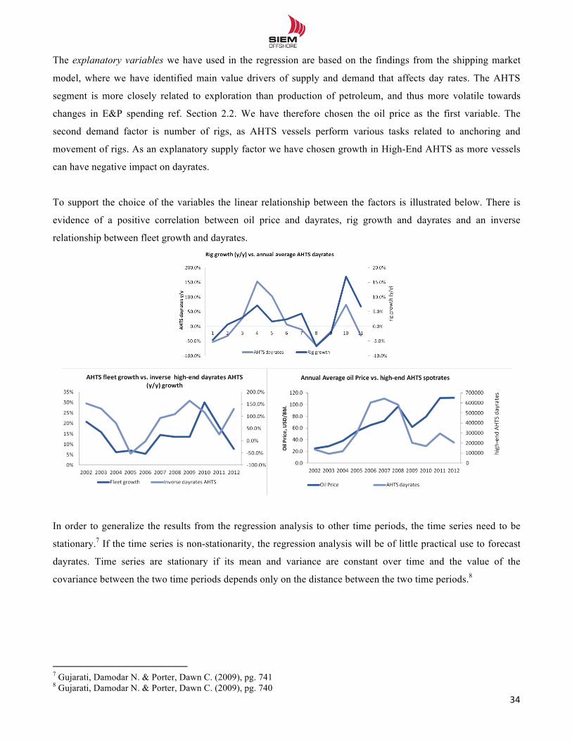
!!
34!!
The explanatory variables we have used in the regression are based on the findings from the shipping market
model, where we have identified main value drivers of supply and demand that affects day rates. The AHTS
segment is more closely related to exploration than production of petroleum, and thus more volatile towards
changes in E&P spending ref. Section 2.2. We have therefore chosen the oil price as the first variable. The
second demand factor is number of rigs, as AHTS vessels perform various tasks related to anchoring and
movement of rigs. As an explanatory supply factor we have chosen growth in High-End AHTS as more vessels
can have negative impact on dayrates.
To support the choice of the variables the linear relationship between the factors is illustrated below. There is
evidence of a positive correlation between oil price and dayrates, rig growth and dayrates and an inverse
relationship between fleet growth and dayrates.
In order to generalize the results from the regression analysis to other time periods, the time series need to be
stationary.7 If the time series is non-stationarity, the regression analysis will be of little practical use to forecast
dayrates. Time series are stationary if its mean and variance are constant over time and the value of the
covariance between the two time periods depends only on the distance between the two time periods.8
!!!!!!!!!!!!!!!!!!!!!!!!!!!!!!!!!!!!!!!!!!!!!!!!!!!!!!!!!!!!!7 Gujarati, Damodar N. & Porter, Dawn C. (2009), pg. 741 8 Gujarati, Damodar N. & Porter, Dawn C. (2009), pg. 740
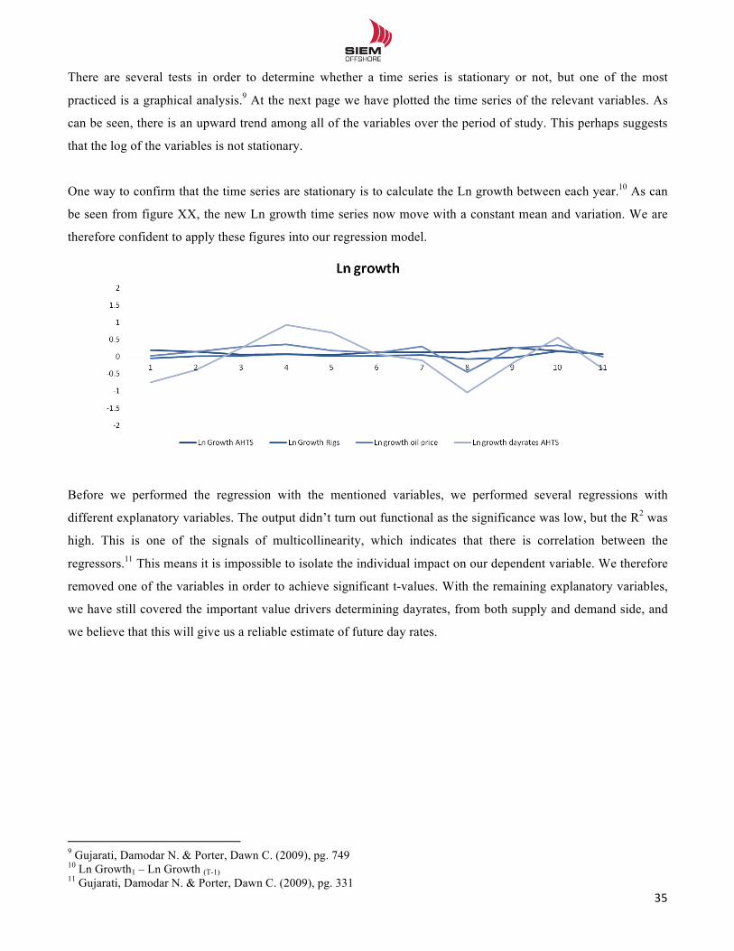
!!
35!!
There are several tests in order to determine whether a time series is stationary or not, but one of the most
practiced is a graphical analysis.9 At the next page we have plotted the time series of the relevant variables. As
can be seen, there is an upward trend among all of the variables over the period of study. This perhaps suggests
that the log of the variables is not stationary.
One way to confirm that the time series are stationary is to calculate the Ln growth between each year.10 As can
be seen from figure XX, the new Ln growth time series now move with a constant mean and variation. We are
therefore confident to apply these figures into our regression model.
Before we performed the regression with the mentioned variables, we performed several regressions with
different explanatory variables. The output didn’t turn out functional as the significance was low, but the R2 was
high. This is one of the signals of multicollinearity, which indicates that there is correlation between the
regressors.11 This means it is impossible to isolate the individual impact on our dependent variable. We therefore
removed one of the variables in order to achieve significant t-values. With the remaining explanatory variables,
we have still covered the important value drivers determining dayrates, from both supply and demand side, and
we believe that this will give us a reliable estimate of future day rates.
!!!!!!!!!!!!!!!!!!!!!!!!!!!!!!!!!!!!!!!!!!!!!!!!!!!!!!!!!!!!!9 Gujarati, Damodar N. & Porter, Dawn C. (2009), pg. 749 10 Ln Growth1 – Ln Growth (T-1) 11 Gujarati, Damodar N. & Porter, Dawn C. (2009), pg. 331
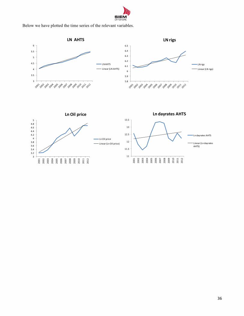
!!
36!!
Below we have plotted the time series of the relevant variables.
3
3.5
4
4.5
5
5.5
6
LN##AHTS#
LN(AHTS
Linear((LN(AHTS)
5.8
5.9
6
6.1
6.2
6.3
6.4
6.5
LN#rigs
LN(rigs
Linear((LN(rigs)
33.23.43.63.84
4.24.44.64.85
2001
2002
2003
2004
2005
2006
2007
2008
2009
2010
2011
2012
Ln#Oil#price
Ln.Oil.price
Linear.(Ln.Oil.price)
11
11.5
12
12.5
13
13.5
2001
2002
2003
2004
2005
2006
2007
2008
2009
2010
2011
2012
Ln#dayrates#AHTS
Ln.dayrates.AHTS
Linear.(Ln.dayrates.AHTS)
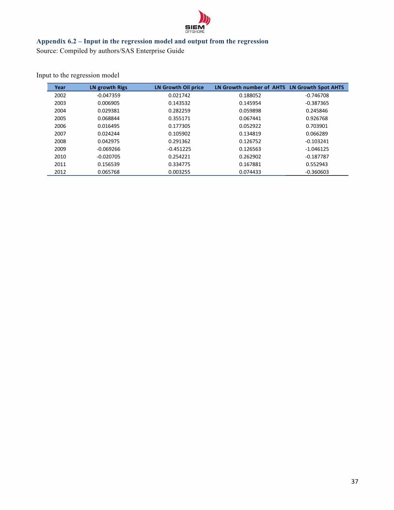
!!
37!!
Appendix 6.2 – Input in the regression model and output from the regression Source: Compiled by authors/SAS Enterprise Guide
Input to the regression model
Year LN'growth'Rigs LN'Growth'Oil'price LN'Growth'number'of''AHTS LN'Growth'Spot'AHTS2002 #0.047359 0.021742 0.188052 #0.7467082003 0.006905 0.143532 0.145954 #0.3873652004 0.029381 0.282259 0.059898 0.2458462005 0.068844 0.355171 0.067441 0.9267682006 0.016495 0.177305 0.052922 0.7039012007 0.024244 0.105902 0.134819 0.0662892008 0.042975 0.291362 0.126752 #0.1032412009 #0.069266 #0.451225 0.126563 #1.0461252010 #0.020705 0.254221 0.262902 #0.1877872011 0.156539 0.334775 0.167881 0.5529432012 0.065768 0.003255 0.074433 #0.360603
!!
38!!
Output from SAS Enterprise
In order to determine whether the results are a good approximation to forecast day rates, one option is to test
them with reference to a zero or alternative hypothesis.12 The decision whether to reject or not to reject the null
hypothesis can be determined by confidence interval and test of significance. For a confidence level of 90% the
P-value must be below 0.1 to reject the null hypothesis. If the parameters fall within the confidence interval, this
is an indication of a linear relationship between the dependent variable and the explanatory variables and the day
rate.13
!!!!!!!!!!!!!!!!!!!!!!!!!!!!!!!!!!!!!!!!!!!!!!!!!!!!!!!!!!!!!12 Gujarati, Damodar N. & Porter, Dawn C. (2009), pg. 113 13 Gujarati, Damodar N. & Porter, Dawn C. (2009), pg. 114
Linear Regression Results
The REG Procedure
Model: Linear_Regression_Model
Dependent Variable: LN Growth Spot AHTS
Sum$of MeanSquares Square
Model 3 2.8928 0.96427 8.44 0.01Error 7 0.79985 0.11426Corrected$Total 10 3.69265
Analysis$of$Variance
Source DF F$Value Pr$>$F
Number of Observations Read 11Number of Observations Used 11
Root$MSE 0.33803 R>Square 0.7834Dependent$Mean ,0.0306 Adj$R>Sq 0.6906Coeff$Var ,1106.4
Parameter StandardEstimate Error
Intercept 1 0.12383 0.25838 0.48 0.6464LN$growth$Rigs 1 1.73673 2.41642 0.72 0.4956LN$Growth$Oil$price 1 1.74896 0.62727 2.79 0.027LN$Growth$number$of$AHTS 1 ,3.43081 1.77475 ,1.93 0.0945
Variable DF t$Value Pr$>$|t|
Parameter$Estimates
!!
39!!
Appendix 6.3 – Analyst forecast of AHTS and PSV dayrates Source: Compiled by authors / Pareto Securities / ABG Sundal Collier
In the following we have listet investment banks estimates for dayrates. These are the only companies that estimate specific number, but other investment banks and brokerage firms have estimated future growth and development from todays level. These have been taken into consideration in our forecast of dayrates.
Forecast)AHTS)dayrates 2013 2014 2015Pareto)Securities)AHTS)25.000)bhp)(USD) 46,711))))))))))))))))))) 57,895))))))))))))))))))) 65,789)))))))))))))))))))Pareto)Securities)AHTS)18.000)bhp)(USD) 40,570))))))))))))))))))) 50,000))))))))))))))))))) 57,018)))))))))))))))))))ABG)Sundal)Collier)18.000+)bhp,)(USD) 46,316))))))))))))))))))) 54,035))))))))))))))))))) N/AAverage 44,532))))))))))))))))))) 53,977))))))))))))))))))) 61,404)))))))))))))))))))
Forecast)PSV)dayrates 2013 2014 2015Pareto)Securities)PSV)3000)dwt)(USD) 20,395))))))))))))))))))) 23,465))))))))))))))))))) 23,684)))))))))))))))))))Pareto)Securities)PSV)4500)dwt)(USD) 26,096))))))))))))))))))) 26,754))))))))))))))))))) 28,070)))))))))))))))))))Average 23,246))))))))))))))))))) 25,110))))))))))))))))))) 25,877)))))))))))))))))))
!!
40!!
Appendix 6.4 – IRR calculations, Subsea dayrates Source: Compiled by authors / Øyvind Hagen, analyst at ABG Sundal Collier
Year 0 1 2 3 4 5 6 7 8 9 10Utilization 98% 98% 98% 98% 98% 98% 98% 98% 98% 98%Number:of:days 365 365 365 365 365 365 365 365 365 365Growth:in:dayrates 5.0% 5.0% 5.0% 5.0% 2.0% 2.0% 2.0% 2.0% 2.0% 2.0%Dayrate 69825 73316.25 76982.0625 80831.16563 82447.78894 84096.74472 85778.67961 87494.2532 89244.13827 91029.02103Growth:in:OPEX 5.0% 5.0% 2.5% 2.5% 2.5% 2.5% 2.5% 2.5% 2.5% 2.5%OPEX (12,290,000)::::::: (12,904,500.00): (13,227,112.50): (13,557,790.31): (13,896,735.07): (14,244,153.45): (14,600,257.28): (14,965,263.72): (15,339,395.31): (15,722,880.19):
Cashflow:before:tax ############# 12,686,402.50::: 13,320,722.63::: 14,309,371.26::: 15,355,517.63::: 15,594,839.03::: 15,837,252.14::: 16,082,776.41::: 16,331,430.66::: 16,583,232.95::: 16,838,200.63:::Tax 1,776,096.35::::: 1,864,901.17::::: 2,003,311.98::::: 2,149,772.47::::: 2,183,277.46::::: 2,217,215.30::::: 2,251,588.70::::: 2,286,400.29::::: 2,321,652.61::::: 2,357,348.09:::::Cash:flow:after:tax ############# 10,910,306.15::: 11,455,821.46::: 12,306,059.28::: 13,205,745.16::: 13,411,561.57::: 13,620,036.84::: 13,831,187.72::: 14,045,030.36::: 14,261,580.34::: 14,480,852.54:::
11 12 13 14 15 16 17 18 19 2098% 98% 98% 98% 98% 98% 98% 98% 98% 98%365 365 365 365 365 365 365 365 365 3652.0% 2.0% 2.0% 2.0% 2.0% 2.0% 2.0% 2.0% 2.0% 2.0%
92849.60145 94706.59348 96600.72535 98532.73986 100503.3947 102513.4625 104563.7318 106655.0064 108788.1066 110963.86872.5% 2.5% 2.5% 2.5% 2.5% 2.5% 2.5% 2.5% 2.5% 2.5%
(16,115,952.20)0000000000 (16,518,851.00)00 (16,931,822.28)0 (17,355,117.83)0 (17,788,995.78)0 (18,233,720.67)0 (18,689,563.69)0 (19,156,802.78)0 (19,635,722.85)0 (20,126,615.92)0
17,096,350.2400000000000 17,357,697.49000 17,622,257.18000 17,890,043.21000 18,161,068.49000 18,435,344.88000 18,712,883.18000 18,993,693.02000 19,277,782.87000 19,565,159.910002,393,489.0300000000000000 2,430,077.65000000 2,467,116.0100000 2,504,606.0500000 2,542,549.5900000 2,580,948.2800000 2,619,803.6400000 2,659,117.0200000 2,698,889.6000000 2,739,122.390000014,702,861.2100000000000 14,927,619.84000 15,155,141.18000 15,385,437.16000 15,618,518.90000 15,854,396.60000 16,093,079.53000 16,334,576.00000 16,578,893.27000 16,826,037.52000
21 22 23 24 25 26 27 28 29 3098% 98% 98% 98% 98% 98% 98% 98% 98% 98%365 365 365 365 365 365 365 365 365 3652.0% 2.0% 2.0% 2.0% 2.0% 2.0% 2.0% 2.0% 2.0% 2.0%
113183.1461 115446.809 117755.7452 120110.8601 122513.0773 124963.3388 127462.6056 130011.8577 132612.0949 135264.33682.5% 2.5% 2.5% 2.5% 2.5% 2.5% 2.5% 2.5% 2.5% 2.5%
(20,629,781.32)0000000000 (21,145,525.85)00 (21,674,164.00)0 (22,216,018.10)0 (22,771,418.55)0 (23,340,704.02)0 (23,924,221.62)0 (24,522,327.16)0 (25,135,385.34)0 (25,763,769.97)0
19,855,830.0300000000000 20,149,797.72000 20,447,066.05000 20,747,636.55000 21,051,509.19000 21,358,682.28000 21,669,152.41000 21,982,914.35000 22,299,961.00000 22,620,283.290002,779,816.2000000000000000 2,820,971.68000000 2,862,589.2500000 2,904,669.1200000 2,947,211.2900000 2,990,215.5200000 3,033,681.3400000 3,077,608.0100000 3,121,994.5400000 3,166,839.660000017,076,013.8200000000000 17,328,826.04000 17,584,476.80000 17,842,967.43000 18,104,297.90000 18,368,466.76000 18,635,471.07000 18,905,306.34000 19,177,966.46000 19,453,443.63000
Days 365Investment (105,000,000)33333333Dayrate,3ultimo32012 66,500333333333333333333333Utilization 0.98Taxrate 0.14IRR 12%
Input&and&results
!!
41!!
Appendix 6.5 – Value of term contracts Source: Compiled by authors/Fearnley Securities/SIOFF annual reports and company presentations
Dayrates is calculated based on the contract value and the number of days between contract signing and expiry.
All numbers in USD.
Vessel%name Reported%value Contract%start Contract%end Estimated%UtilizationEstimated%dayratesAHTS USD USD
Siem Emerald 70,000,000 1/1/2011 1/1/2015 100% 48,611Siem Pearl 70,000,000 1/1/2011 1/1/2015 100% 48,611Siem Diamond 70,000,000 1/1/2011 1/1/2015 100% 48,611Siem Ruby 100,000,000 7/1/2012 7/1/2016 100% 69,444Siem Sapphire 70,000,000 1/1/2011 1/1/2015 100% 48,611
PSVSiem Symphony 47,000,000 7/1/2014 7/1/2018 100% 32,639Hugin Explorer 45,000,000 4/1/2012 4/1/2018 100% 20,833Siem Supplier Estimate 4/1/2013 4/1/2016 100% 24,561Siem Sailor Estimate 12/31/2013 100% 28,947Siem Pilot Estimate 12/31/2013 100% 28,947Siem Mariner Estimate 1/4/2013 100% 28,947Siddis Skipper Estimate 12/31/2013 100% 25,000Siem Sasha Estimate 1/7/2013 100% 25,000Siem Louisa Estimate 1/7/2013 100% 25,000
FCV/FSVSiem Piata 17,500,000 1/2/2011 1/2/2019 100% 6,076Siem Pendotiba 17,500,000 1/2/2012 1/2/2020 100% 6,076Siem Caetes 23,000,000 1/2/2011 1/2/2019 100% 7,986Siem Carajas 23,000,000 1/2/2012 1/2/2020 100% 7,986Norsul Parati Estimate 1/7/2014 100% 3,993Capela Estimate 1/7/2014 100% 3,993Norsul Paropria Estimate 1/7/2014 100% 3,993Parnaiba Estimate 1/7/2014 100% 3,993
OSRVSiem Maragogi 94,000,000 1/1/2013 1/1/2021 100% 32,639Siem Marataizes 94,000,000 1/1/2013 1/1/2021 100% 32,639
OSCVSiem Daya Estimate 1/7/2013 1/7/2018 100% 73,000
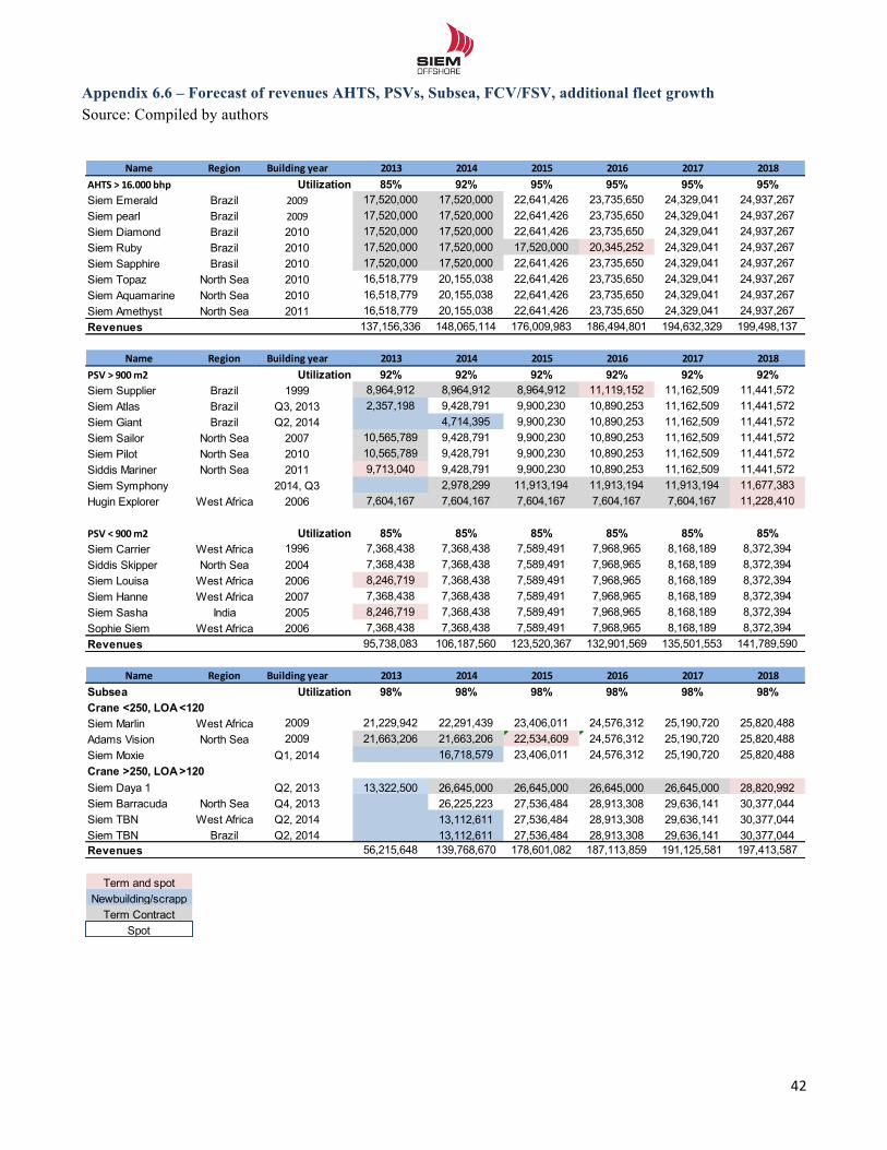
!!
42!!
Appendix 6.6 – Forecast of revenues AHTS, PSVs, Subsea, FCV/FSV, additional fleet growth Source: Compiled by authors
Name Region Building.year 2013 2014 2015 2016 2017 2018AHTS.>.16.000.bhp 85% 92% 95% 95% 95% 95%Siem Emerald Brazil 2009 17,520,000 17,520,000 22,641,426 23,735,650 24,329,041 24,937,267Siem pearl Brazil 2009 17,520,000 17,520,000 22,641,426 23,735,650 24,329,041 24,937,267Siem Diamond Brazil 2010 17,520,000 17,520,000 22,641,426 23,735,650 24,329,041 24,937,267Siem Ruby Brazil 2010 17,520,000 17,520,000 17,520,000 20,345,252 24,329,041 24,937,267Siem Sapphire Brasil 2010 17,520,000 17,520,000 22,641,426 23,735,650 24,329,041 24,937,267Siem Topaz North Sea 2010 16,518,779 20,155,038 22,641,426 23,735,650 24,329,041 24,937,267Siem Aquamarine North Sea 2010 16,518,779 20,155,038 22,641,426 23,735,650 24,329,041 24,937,267Siem Amethyst North Sea 2011 16,518,779 20,155,038 22,641,426 23,735,650 24,329,041 24,937,267Revenues 137,156,336 148,065,114 176,009,983 186,494,801 194,632,329 199,498,137
Name Region Building.year 2013 2014 2015 2016 2017 2018PSV.>.900.m2 92% 92% 92% 92% 92% 92%Siem Supplier Brazil 1999 8,964,912 8,964,912 8,964,912 11,119,152 11,162,509 11,441,572Siem Atlas Brazil Q3, 2013 2,357,198 9,428,791 9,900,230 10,890,253 11,162,509 11,441,572Siem Giant Brazil Q2, 2014 4,714,395 9,900,230 10,890,253 11,162,509 11,441,572Siem Sailor North Sea 2007 10,565,789 9,428,791 9,900,230 10,890,253 11,162,509 11,441,572Siem Pilot North Sea 2010 10,565,789 9,428,791 9,900,230 10,890,253 11,162,509 11,441,572Siddis Mariner North Sea 2011 9,713,040 9,428,791 9,900,230 10,890,253 11,162,509 11,441,572Siem Symphony 2014, Q3 2,978,299 11,913,194 11,913,194 11,913,194 11,677,383Hugin Explorer West Africa 2006 7,604,167 7,604,167 7,604,167 7,604,167 7,604,167 11,228,410
PSV.<.900.m2 85% 85% 85% 85% 85% 85%Siem Carrier West Africa 1996 7,368,438 7,368,438 7,589,491 7,968,965 8,168,189 8,372,394Siddis Skipper North Sea 2004 7,368,438 7,368,438 7,589,491 7,968,965 8,168,189 8,372,394Siem Louisa West Africa 2006 8,246,719 7,368,438 7,589,491 7,968,965 8,168,189 8,372,394Siem Hanne West Africa 2007 7,368,438 7,368,438 7,589,491 7,968,965 8,168,189 8,372,394Siem Sasha India 2005 8,246,719 7,368,438 7,589,491 7,968,965 8,168,189 8,372,394Sophie Siem West Africa 2006 7,368,438 7,368,438 7,589,491 7,968,965 8,168,189 8,372,394Revenues 95,738,083 106,187,560 123,520,367 132,901,569 135,501,553 141,789,590
Name Region Building.year 2013 2014 2015 2016 2017 2018Subsea 98% 98% 98% 98% 98% 98%Crane <250, LOA <120Siem Marlin West Africa 2009 21,229,942 22,291,439 23,406,011 24,576,312 25,190,720 25,820,488Adams Vision North Sea 2009 21,663,206 21,663,206 22,534,609 24,576,312 25,190,720 25,820,488Siem Moxie Q1, 2014 16,718,579 23,406,011 24,576,312 25,190,720 25,820,488Crane >250, LOA >120Siem Daya 1 Q2, 2013 13,322,500 26,645,000 26,645,000 26,645,000 26,645,000 28,820,992Siem Barracuda North Sea Q4, 2013 26,225,223 27,536,484 28,913,308 29,636,141 30,377,044Siem TBN West Africa Q2, 2014 13,112,611 27,536,484 28,913,308 29,636,141 30,377,044Siem TBN Brazil Q2, 2014 13,112,611 27,536,484 28,913,308 29,636,141 30,377,044Revenues 56,215,648 139,768,670 178,601,082 187,113,859 191,125,581 197,413,587
Term and spotNewbuilding/scrapp
Term ContractSpot
Utilization
Utilization
Utilization
Utilization
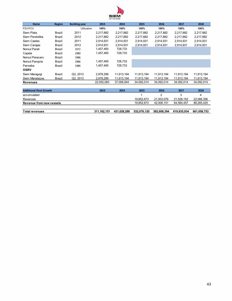
!!
43!!
Name Region Building.year 2013 2014 2015 2016 2017 2018FSV/FCV 100% 100% 100% 100% 100% 100%Siem Piata Brazil 2011 2,217,882 2,217,882 2,217,882 2,217,882 2,217,882 2,217,882Siem Pendotiba Brazil 2012 2,217,882 2,217,882 2,217,882 2,217,882 2,217,882 2,217,882Siem Caetes Brazil 2011 2,914,931 2,914,931 2,914,931 2,914,931 2,914,931 2,914,931Siem Carajas Brazil 2012 2,914,931 2,914,931 2,914,931 2,914,931 2,914,931 2,914,931Norsul Parati Brazil 1972 1,457,465 728,733Capela Brazil 1980 1,457,465 728,733Norsul Paracaru Brazil 1986Norsul Paropria Brazil 1986 1,457,465 728,733Parnaiba Brazil 1986 1,457,465 728,733OSRVSiem Maragogi Brazil Q2, 2013 2,978,299 11,913,194 11,913,194 11,913,194 11,913,194 11,913,194Siem Marataizes Brazil Q2, 2013 2,978,299 11,913,194 11,913,194 11,913,194 11,913,194 11,913,194Revenues 22,052,083 37,006,944 34,092,014 34,092,014 34,092,014 34,092,014
2013 2014 2015 2016 2017 2018Vessels, accumulated 1 2 3 4Revenues 19,852,673 21,003,076 21,528,152 22,066,356
19,852,673 42,006,151 64,584,457 88,265,425
Total revenues 311,162,151 431,028,288 532,076,120 582,608,394 619,935,934 661,058,753
Additional.fleet.Growth
Revenue from new vessels
Utilization
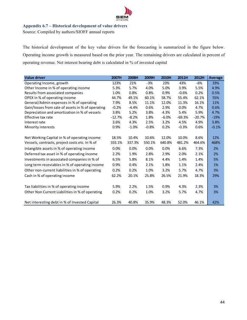
!!
44!!
Appendix 6.7 – Historical development of value drivers Source: Compiled by authors/SIOFF annual reports
The historical development of the key value drivers for the forecasting is summarized in the figure below.
Operating income growth is measured based on the prior year. The remaining drivers are calculated in percent of
operating revenue. Net interest bearing debt is calculated in % of invested capital
Value&driver 2007H 2008H 2009H 2010H 2011H 2012H AverageOperating*Income,*growth 123% 21% 63% 23% 43% 66% 33%Other*Income*in*%*of*operating*income 5.3% 5.7% 4.0% 5.0% 3.9% 5.5% 4.9%Results*from*associated*companies 1.0% 0.8% 0.8% 0.9% 60.6% 0.2% 0.5%OPEX*in*%*of*operating*income 44.7% 49.1% 60.1% 58.7% 55.4% 62.1% 55%General/Admin*expences*in*%*of*operating* 7.9% 8.5% 11.1% 12.0% 11.3% 16.1% 11%Gain/losses*from*sale*of*assets*in*%*of*operating* 60.2% 64.4% 0.6% 2.9% 0.0% 4.7% 0.6%Depreciation*and*amortization*in*%*of*vessels* 3.8% 5.2% 3.8% 4.3% 5.4% 5.9% 4.7%Effective*tax*rate 612.7% 68.2% 1.8% 66.0% 669.3% 620.7% 619%Interest*rate 3.6% 4.3% 2.5% 3.2% 4.5% 4.9% 3.8%Minority*interests 0.9% 61.0% 60.8% 0.2% 60.3% 0.6% 60.1%
Net*Working*Capital*in*%*of*operating*income 18.5% 10.4% 10.6% 12.0% 10.0% 8.6% 12%Vessels,*contracts,*project*costs*etc.*In*%*of* 333.1% 337.3% 550.1% 640.8% 481.2% 464.6% 468%Intangible*assets*in*%*of*operating*income 0.0% 0.0% 0.0% 0.0% 6.6% 7.3% 2%Deferred*tax*asset*in*%*of*operating*income 2.2% 1.9% 2.8% 2.9% 2.0% 2.1% 2%Investments*in*associated*companies*in*%*of* 6.5% 5.8% 8.1% 4.4% 1.4% 1.4% 5%Long*term*receviables*in*%*of*operating*income 0.9% 0.4% 2.1% 1.8% 1.1% 2.4% 1%Other*non6current*liabilities*in*%*of*operating* 0.2% 0.2% 1.0% 3.2% 5.7% 4.7% 3%Cash*in*%*of*operating*income 62.2% 20.1% 25.8% 26.5% 21.9% 18.3% 29%
Tax*liabilities*in*%*of*operating*income 5.9% 2.2% 1.5% 0.9% 4.3% 2.3% 3%Other*Non*Current*Liabilities*in*%*of*operating* 0.2% 0.2% 1.0% 3.2% 5.7% 4.7% 3%
Net*interesting*debt*in*%*of*Invested*Capital 26.3% 40.8% 35.9% 48.3% 52.0% 46.1% 42%
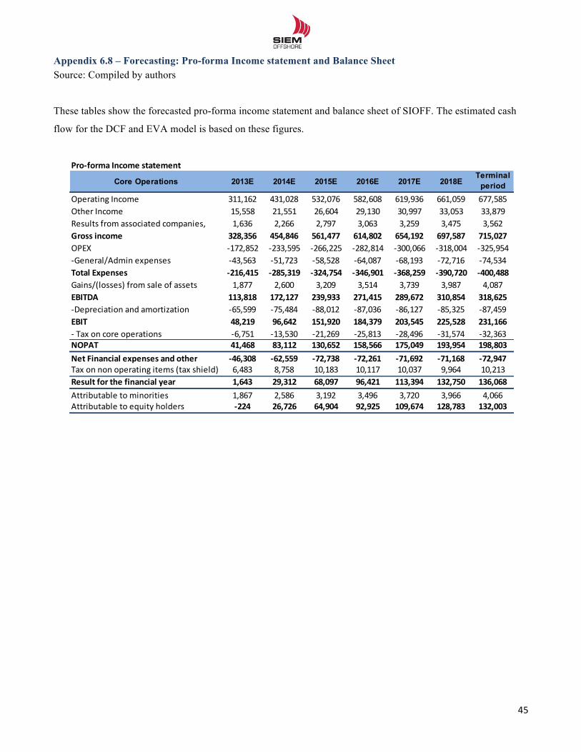
!!
45!!
Appendix 6.8 – Forecasting: Pro-forma Income statement and Balance Sheet Source: Compiled by authors
These tables show the forecasted pro-forma income statement and balance sheet of SIOFF. The estimated cash
flow for the DCF and EVA model is based on these figures.
Pro$forma(Income(statement
Core Operations 2013E 2014E 2015E 2016E 2017E 2018ETerminal
periodOperating*Income 311,162 431,028 532,076 582,608 619,936 661,059 677,585Other*Income 15,558 21,551 26,604 29,130 30,997 33,053 33,879Results*from*associated*companies,* 1,636 2,266 2,797 3,063 3,259 3,475 3,562Gross(income 328,356 454,846 561,477 614,802 654,192 697,587 715,027OPEX D172,852 D233,595 D266,225 D282,814 D300,066 D318,004 D325,954DGeneral/Admin*expenses D43,563 D51,723 D58,528 D64,087 D68,193 D72,716 D74,534Total(Expenses $216,415 $285,319 $324,754 $346,901 $368,259 $390,720 $400,488Gains/(losses)*from*sale*of*assets 1,877 2,600 3,209 3,514 3,739 3,987 4,087EBITDA 113,818 172,127 239,933 271,415 289,672 310,854 318,625DDepreciation*and*amortization D65,599 D75,484 D88,012 D87,036 D86,127 D85,325 D87,459EBIT 48,219 96,642 151,920 184,379 203,545 225,528 231,166D*Tax*on*core*operations D6,751 D13,530 D21,269 D25,813 D28,496 D31,574 D32,363NOPAT 41,468 83,112 130,652 158,566 175,049 193,954 198,803Net(Financial(expenses(and(other $46,308 $62,559 $72,738 $72,261 $71,692 $71,168 $72,947Tax*on*non*operating*items*(tax*shield) 6,483 8,758 10,183 10,117 10,037 9,964 10,213Result(for(the(financial(year 1,643 29,312 68,097 96,421 113,394 132,750 136,068Attributable*to*minorities 1,867 2,586 3,192 3,496 3,720 3,966 4,066Attributable*to*equity*holders $224 26,726 64,904 92,925 109,674 128,783 132,003
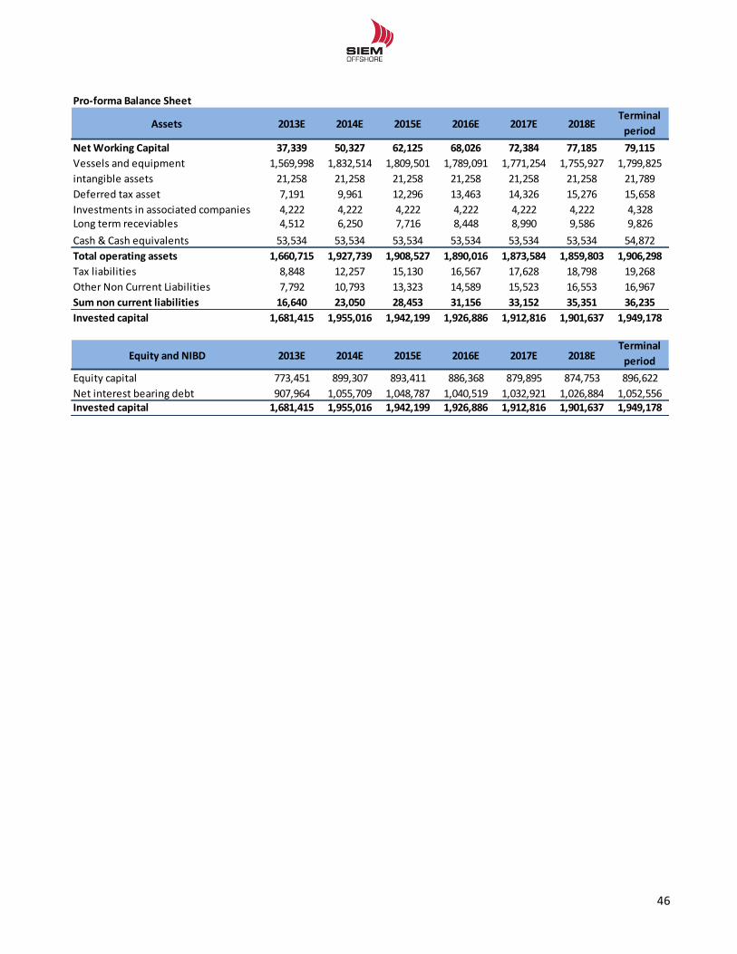
!!
46!!
Pro$forma(Balance(Sheet
Assets 2013E 2014E 2015E 2016E 2017E 2018ETerminal(period
Net(Working(Capital 37,339 50,327 62,125 68,026 72,384 77,185 79,115Vessels%and%equipment 1,569,998 1,832,514 1,809,501 1,789,091 1,771,254 1,755,927 1,799,825intangible%assets 21,258 21,258 21,258 21,258 21,258 21,258 21,789Deferred%tax%asset 7,191 9,961 12,296 13,463 14,326 15,276 15,658Investments%in%associated%companies 4,222 4,222 4,222 4,222 4,222 4,222 4,328Long%term%receviables 4,512 6,250 7,716 8,448 8,990 9,586 9,826Cash%&%Cash%equivalents 53,534 53,534 53,534 53,534 53,534 53,534 54,872Total(operating(assets 1,660,715 1,927,739 1,908,527 1,890,016 1,873,584 1,859,803 1,906,298Tax%liabilities 8,848 12,257 15,130 16,567 17,628 18,798 19,268Other%Non%Current%Liabilities 7,792 10,793 13,323 14,589 15,523 16,553 16,967Sum(non(current(liabilities 16,640 23,050 28,453 31,156 33,152 35,351 36,235Invested(capital 1,681,415 1,955,016 1,942,199 1,926,886 1,912,816 1,901,637 1,949,178
Equity(and(NIBD 2013E 2014E 2015E 2016E 2017E 2018ETerminal(period
Equity%capital 773,451 899,307 893,411 886,368 879,895 874,753 896,622Net%interest%bearing%debt 907,964 1,055,709 1,048,787 1,040,519 1,032,921 1,026,884 1,052,556Invested(capital 1,681,415 1,955,016 1,942,199 1,926,886 1,912,816 1,901,637 1,949,178
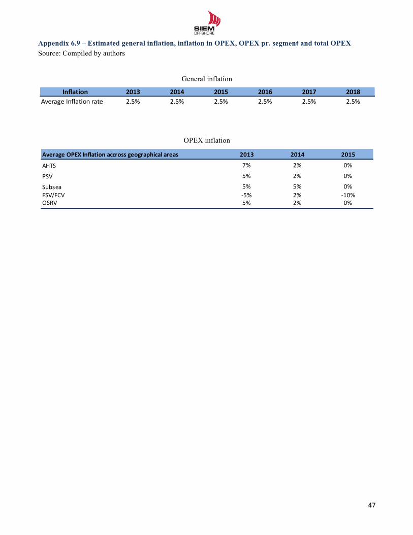
!!
47!!
Appendix 6.9 – Estimated general inflation, inflation in OPEX, OPEX pr. segment and total OPEX Source: Compiled by authors
General inflation
OPEX inflation
Inflation 2013 2014 2015 2016 2017 2018Average'Inflation'rate 2.5% 2.5% 2.5% 2.5% 2.5% 2.5%
Average'OPEX'Inflation'accross'geographical'areas 2013 2014 2015
AHTS 7% 2% 0%
PSV 5% 2% 0%
Subsea 5% 5% 0%FSV/FCV 45% 2% 410%OSRV 5% 2% 0%
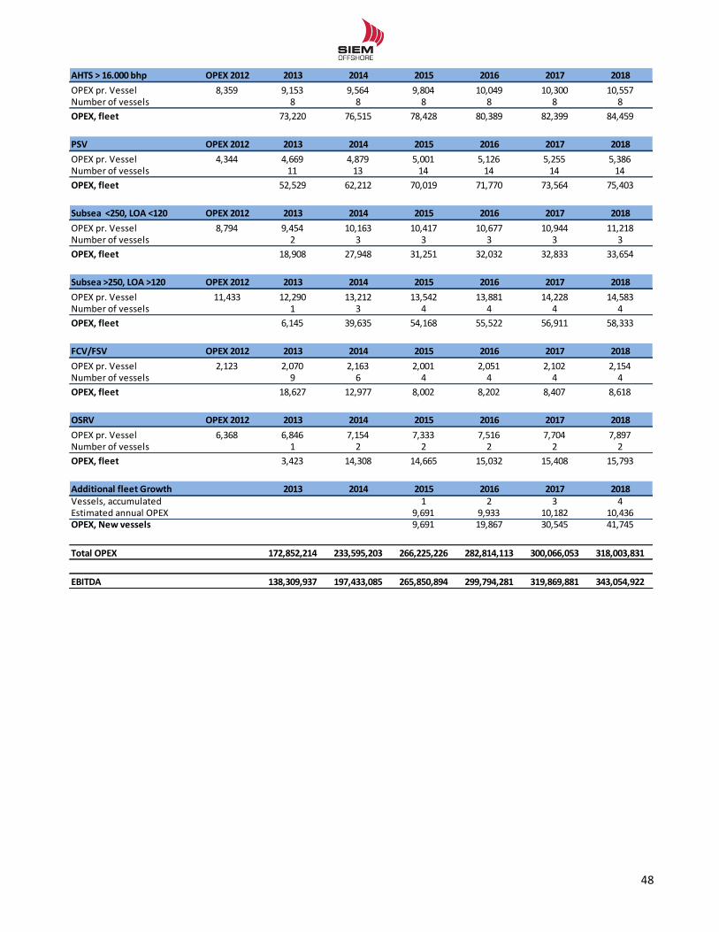
!!
48!!
AHTS%>%16.000%bhp OPEX%2012 2013 2014 2015 2016 2017 2018
OPEX%pr.%Vessel 8,359 9,153 9,564 9,804 10,049 10,300 10,557Number%of%vessels 8 8 8 8 8 8OPEX,%fleet 73,220 76,515 78,428 80,389 82,399 84,459
PSV OPEX%2012 2013 2014 2015 2016 2017 2018
OPEX%pr.%Vessel 4,344 4,669 4,879 5,001 5,126 5,255 5,386Number%of%vessels 11 13 14 14 14 14OPEX,%fleet 52,529 62,212 70,019 71,770 73,564 75,403
Subsea%%<250,%LOA%<120 OPEX%2012 2013 2014 2015 2016 2017 2018
OPEX%pr.%Vessel 8,794 9,454 10,163 10,417 10,677 10,944 11,218Number%of%vessels 2 3 3 3 3 3OPEX,%fleet 18,908 27,948 31,251 32,032 32,833 33,654
Subsea%>250,%LOA%>120 OPEX%2012 2013 2014 2015 2016 2017 2018
OPEX%pr.%Vessel 11,433 12,290 13,212 13,542 13,881 14,228 14,583Number%of%vessels 1 3 4 4 4 4OPEX,%fleet 6,145 39,635 54,168 55,522 56,911 58,333
FCV/FSV OPEX%2012 2013 2014 2015 2016 2017 2018
OPEX%pr.%Vessel 2,123 2,070 2,163 2,001 2,051 2,102 2,154Number%of%vessels 9 6 4 4 4 4OPEX,%fleet 18,627 12,977 8,002 8,202 8,407 8,618
OSRV OPEX%2012 2013 2014 2015 2016 2017 2018
OPEX%pr.%Vessel 6,368 6,846 7,154 7,333 7,516 7,704 7,897Number%of%vessels 1 2 2 2 2 2OPEX,%fleet 3,423 14,308 14,665 15,032 15,408 15,793
Additional%fleet%Growth 2013 2014 2015 2016 2017 2018Vessels,%accumulated 1 2 3 4Estimated%annual%OPEX 9,691 9,933 10,182 10,436OPEX,%New%vessels 9,691 19,867 30,545 41,745
Total%OPEX 172,852,214 233,595,203 266,225,226 282,814,113 300,066,053 318,003,831
EBITDA 138,309,937 197,433,085 265,850,894 299,794,281 319,869,881 343,054,922
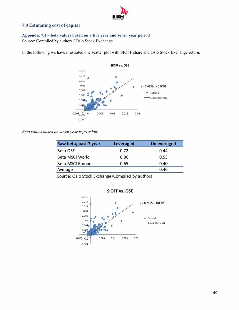
!!
49!!
7.0 Estimating cost of capital
Appendix 7.1 – beta values based on a five year and seven year period Source: Compiled by authors / Oslo Stock Exchange
In the following we have illustrated one scatter plot with SIOFF share and Oslo Stock Exchange return.
Beta values based on seven year regression:
y"="0.6958x"+"0.0002
-0.004
-0.002
0
0.002
0.004
0.006
0.008
0.01
0.012
0.014
0.016
-0.005 0 0.005 0.01 0.015 0.02
SIOFF%vs.%OSE
Series1
Linear"(Series1)
Raw$beta,$past$7$year$ Leveraged UnleveragedBeta%OSE 0.72 0.44Beta%MSCI%World 0.86 0.53Beta%MSCI%Europe 0.65 0.40Average 0.46Source:%Oslo%Stock%Exchange/Compiled%by%authors
y"="0.7232x"+"0.0002
+0.004
+0.002
0
0.002
0.004
0.006
0.008
0.01
0.012
0.014
0.016
+0.005 0 0.005 0.01 0.015 0.02
SIOFF%vs.%OSE
Series1
Linear"(Series1)
!!
50!!
Appendix 7.2 – Beta from comparable companies Source: Compiled by authors / Reuters Financial
Reuters'raw'beta''Leveraged'
beta'NIBD/Invested'
capitalUnleveraged'
betaHavila&Shipping &&&&&&&&&&&&&&&&&&0.58& 68% 0.21Farstad&Shipping &&&&&&&&&&&&&&&&&&0.69& 45% 0.41DOF &&&&&&&&&&&&&&&&&&0.65& 71% 0.21Solstad&Offshore &&&&&&&&&&&&&&&&&&0.82& 17% 0.70Average 0.38
!!
51!!
Appendix 7.3 – Fundamental beta analysis Source: Compiled by authors
Fundamental Beta analysisTypes of operating risk Assessment of risk level The firms ability to manage operating risk
External risk Not sufficient- Oil price and E&P spending - High Risk of fluctuating oil price- Orderbook of new vessels - High High orderbook of PSVs- Legislation/regulatory changes - High Regulatory preassure in Brazil and West Africa
Strategic risk Not sufficient
- Rivalry among competitors - High Many competitors in the same market- Suppliers power - Medium Tight labour market, limited yards for some segments
- Customers power - Medium Customers can choose between many owners
- Substitute products - Low No available substitutes- Threat of entry - Medium High for PSV, medium for AHTS and Subsea- Market Growth - Medium Weak market, but improvements expected- Cost inflation - High OPEX expected to increase due to regulations- Ability to adjust prices - High Price takers, can not influence prices
Operating risk Reasonable- Exploiting fleet facilities, utilization - Medium Weak utilization in 2013, expected to improve- Quality of management - Low Good management, see internal analysis- Choice of cost structure - High High degree of fixed costs- Prodcut innovation - Medium Early adaptors of new technology
- Quality of fleet - Low Low average age, modern vessels, diversified fleet- Newbuilding risk - Medium Low risk for Norwegian built vessels, medium for Brazil
Types of financial risk Assessment of risk level The firms ability to manage financial risk- Financial leverage - Low Low gearing compared to the industry- Access to financial markets - Low Good access to new debt facilities
Loan Characteristics- Variable interest rate - Medium- Time to maturity - Medium- Foreign currency - Medium
Total assessment of operating risk: High
Total assessment of financial risk: Neutral
!!
52!!
Appendix 7.4 – Implied credit rating Source: Compiled by authors / Plenborg & Petersen Financial Statement analysis / SIOFFs annual reports /
2007 AAA AA A BBB BB B CCCEBIT*Interest0coverage0(x)EBITDA*Interest0coverage0(x)Total0debt/capital0%ROIC0%Operating0income/Revenue0%Implied0rating A
2008 AAA AA A BBB BB B CCCEBIT*Interest0coverage0(x)EBITDA*Interest0coverage0(x)Total0debt/capital0%ROIC0%Operating0income/Revenue0%Implied0rating A*
2009 AAA AA A BBB BB B CCCEBIT*Interest0coverage0(x)EBITDA*Interest0coverage0(x)Total0debt/capital0%ROIC0%Operating0income/Revenue0%Implied0rating A
2010 AAA AA A BBB BB B CCCEBIT*Interest0coverage0(x)EBITDA*Interest0coverage0(x)Total0debt/capital0%ROIC0%Operating0income/Revenue0%Implied0rating BBB
2011 AAA AA A BBB BB B CCCEBIT*Interest0coverage0(x)EBITDA*Interest0coverage0(x)Total0debt/capital0%ROIC0%Operating0income/Revenue0%Implied0rating BB*
2012 AAA AA A BBB BB B CCCEBIT*Interest0coverage0(x)EBITDA*Interest0coverage0(x)Total0debt/capital0%ROIC0%Operating0income/Revenue0%Implied0rating B
!!
53!!
8.0 Valuation
Appendix 8.1 – Valuation: Equity forecast, CAPEX and complete cash flow statement Source: Compiled by authors
Appendix 8.2 – Multiples comparison with Bloomberg Source: Compiled by Authors / Bloomberg
Equity'forecast 2013E 2014E 2015E 2016E 2017E 2018E TerminalEquity'primo '''''''''786,511' '''''''''756,539' '''''''''879,659' '''''''''873,784' '''''''''866,885' '''''''''860,550' '''''''''855,516'Concern'Result '''''''''''''''(864) '''''''''''25,003' '''''''''''62,008' '''''''''''89,897' '''''''''106,603' '''''''''125,659' '''''''''128,800'Dividends ''''''''''(29,108) '''''''''''98,117' ''''''''''(67,883) ''''''''''(96,796) '''''''(112,938) '''''''(130,692) '''''''(107,412)Equity'Ultimo '''''''''756,539' '''''''''879,659' '''''''''873,784' '''''''''866,885' '''''''''860,550' '''''''''855,516' '''''''''876,904'NIBD '''''''''924,659' ''''''1,075,139' ''''''1,067,958' ''''''1,059,526' ''''''1,051,783' ''''''1,045,631' ''''''1,071,772'
Invested'Capital''ultimo 1,681,199'''' 1,954,798'''' 1,941,742'''' 1,926,411'''' 1,912,333'''' 1,901,147'''' 1,948,676''''
CAPEX 2013E 2014E 2015E 2016E 2017E 2018E TerminalIntangible'and'tangible'assets'end'of'period 1,660,637 1,927,659 1,908,359 1,889,845 1,873,413 1,859,632 1,906,123Depreciation 65,599 75,482 88,010 87,031 86,122 85,321 87,454Intangible'and'tangible'assets'beginning'of'period 1,453,978 1,660,637 1,927,659 1,908,359 1,889,845 1,873,413 1,859,632
CAPEX 272,258 342,504 68,710 68,517 69,690 71,540 133,945
Cash'flow'statement 2013E 2014E 2015E 2016E 2017E 2018E TerminalNopat 40,816 82,366 128,879 156,645 173,074 191,917 196,715Depreciation 65,599 75,482 88,010 87,031 86,122 85,321 87,454Change'in'NWC L11,751 L12,982 L11,519 L5,873 L4,344 L4,787 L1,915Change'in'non'current'l iabil ities L4,172 6,404 5,275 2,690 1,990 2,193 877CAPEX L272,258 L342,504 L68,710 L68,517 L69,690 L71,540 L133,945
FCFF J181,767 J191,234 141,936 171,976 187,151 203,103 149,186Change'in'NIBD 252,554 150,480 L7,181 L8,432 L7,743 L6,152 26,141Net'financial'expenses'after'tax L39,825 L54,790 L63,706 L63,281 L62,781 L62,322 L63,880Attributable'to'Minority'interests 1,855 2,573 3,165 3,467 3,690 3,936 4,034
FCFE 29,108 J98,117 67,883 96,796 112,938 130,692 107,412Dividends L29,108 98,117 L67,883 L96,796 L112,938 L130,692 L107,412Cash'surplus 0 0 0 0 0 0 0
EV/EBITDA EV/EBIT EV/Sales P/B
EV/EBITDA EV/EBIT EV/Sales P/B
Bloomberg 8.7 12.8 3.1 0.63 5.8 10.6 2.2 0.58Our estimate 10.4 24.7 3.6 0.66 6.8 12.2 2.6 0.57Difference 1.67 11.89 0.51 0.03 1.09 1.59 0.44 (0.01)
2013 2014
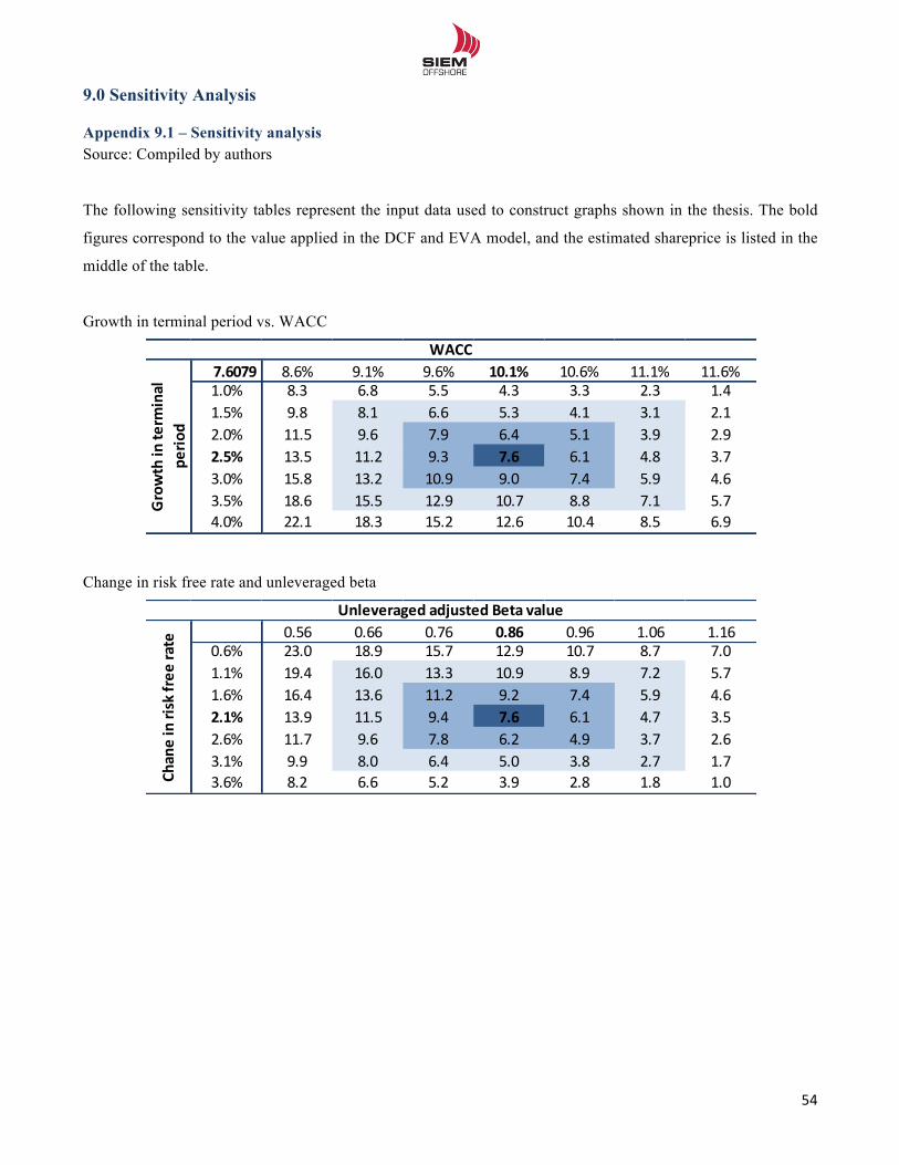
!!
54!!
9.0 Sensitivity Analysis
Appendix 9.1 – Sensitivity analysis Source: Compiled by authors
The following sensitivity tables represent the input data used to construct graphs shown in the thesis. The bold
figures correspond to the value applied in the DCF and EVA model, and the estimated shareprice is listed in the
middle of the table.
Growth in terminal period vs. WACC
Change in risk free rate and unleveraged beta
!!!!!7.6079! 8.6% 9.1% 9.6% 10.1% 10.6% 11.1% 11.6%1.0% 8.3 6.8 5.5 4.3 3.3 2.3 1.41.5% 9.8 8.1 6.6 5.3 4.1 3.1 2.12.0% 11.5 9.6 7.9 6.4 5.1 3.9 2.92.5% 13.5 11.2 9.3 7.6 6.1 4.8 3.73.0% 15.8 13.2 10.9 9.0 7.4 5.9 4.63.5% 18.6 15.5 12.9 10.7 8.8 7.1 5.74.0% 22.1 18.3 15.2 12.6 10.4 8.5 6.9
WACC
Growth!in!te
rminal!
perio
d
0.56% 0.66% 0.76% 0.86% 0.96% 1.06% 1.16%0.6% 23.0 18.9 15.7 12.9 10.7 8.7 7.01.1% 19.4 16.0 13.3 10.9 8.9 7.2 5.71.6% 16.4 13.6 11.2 9.2 7.4 5.9 4.62.1% 13.9 11.5 9.4 7.6 6.1 4.7 3.52.6% 11.7 9.6 7.8 6.2 4.9 3.7 2.63.1% 9.9 8.0 6.4 5.0 3.8 2.7 1.73.6% 8.2 6.6 5.2 3.9 2.8 1.8 1.0Ch
ane%in%risk%free
%rate
Unleveraged%adjusted%Beta%value
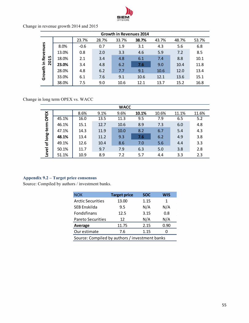
!!
55!!
Change in revenue growth 2014 and 2015
Change in long term OPEX vs. WACC
Appendix 9.2 – Target price consensus Source: Compiled by authors / investment banks.
23.7% 28.7% 33.7% 38.7% 43.7% 48.7% 53.7%8.0% *0.6 0.7 1.9 3.1 4.3 5.6 6.813.0% 0.8 2.0 3.3 4.6 5.9 7.2 8.518.0% 2.1 3.4 4.8 6.1 7.4 8.8 10.123.0% 3.4 4.8 6.2 7.6 9.0 10.4 11.828.0% 4.8 6.2 7.7 9.1 10.6 12.0 13.433.0% 6.1 7.6 9.1 10.6 12.1 13.6 15.138.0% 7.5 9.0 10.6 12.1 13.7 15.2 16.8
Growth/in/Revenues/2014
Growth/in/Reven
ues/
2015
8.6% 9.1% 9.6% 10.1% 10.6% 11.1% 11.6%45.1% 16.0 13.5 11.3 9.5 7.9 6.5 5.246.1% 15.1 12.7 10.6 8.9 7.3 6.0 4.847.1% 14.3 11.9 10.0 8.2 6.7 5.4 4.348.1% 13.4 11.2 9.3 7.6 6.2 4.9 3.849.1% 12.6 10.4 8.6 7.0 5.6 4.4 3.350.1% 11.7 9.7 7.9 6.3 5.0 3.8 2.851.1% 10.9 8.9 7.2 5.7 4.4 3.3 2.3
WACC
Level0of0lon
g5term
0OPEX
NOK Target'price SOC WISArctic)Securities 13.00 1.15 1SEB)Enskilda 9.5 N/A N/AFondsfinans 12.5 3.15 0.8Pareto)Securities 12 N/A N/AAverage 11.75 2.15 0.90Our)estimate 7.6 1.15 0Source:)Compiled)by)authors)/)investment)banks
!!
56!!
10.0 – Summary of interviews with industry professionals
Appendix 10.1 Øyvind Hagen – Analyst at ABG Sundal Collier (Norwegian Investment Bank) Phone interview, 23rd of April 2013
“First of all, there are difference in dayrates depending on whether the vessel is on Spot or Term contract. For
vessels on term contract, contract length etc. affects the rate, but the final contract is determined based on the
current and future market outlook. As North Sea is the only well functioning spot market, rates in other areas are
affected by development in these rates. The most important thing is that rates vary between regions depending on
OPEX. Therefore the margin is similar/equal across region markets. People in the business tend to underestimate
how mobile the vessels are, and vessel owners allocate their vessels constantly depending on the profit outlook.
The most “secure” market is the North Sea. As of OPEX, close to 70% is a result of labour costs. Over the last
years OPEX inflation in Brazil has been as high as 7-10 % yearly, in the North Sea ~3% and West Africa ~5%.
This is a result of the tight labour market, which is expected to continue going forward. OPEX will therefore
increase by 3-7 % depending on the area of operation.”
“For the high-end vessels, the OPEX level is generally higher, as everything is larger and they require more
crew. Maybe the general level is 20-30% higher. The ROCE is also higher for these vessels.”
“When it comes to WACC, it is where simple here at the sell side. We apply a WACC for the OSV industry of
10% flat. I believe that if you ask other investment banks, they will provide you with a similar estimate,
generally between 10-11 %.”
“For the subsea segment there are very little data available for dayrates as the vessels are heterogeneous. Going
forward I believe a moderate growth of 5-10% sounds reasonable. To find the dayrates for SIOFFs Subsea
vessels I would have calculated the IRR. This kind of investment should provide an IRR of 10-12 %, which will
give a reasonable dayrate assumption.”
“For SIEM WIS the stock market is probably not pricing the value as very high. Currently P/B is below 1 and the
industry has been struggling to create returns. None of the petroleum companies have shown any significant
interest in WIS, and the company has not managed to create and develop the technology. Now SIOFF is in the
process of a potential sale, but as everything is so uncertain I would advise you to set the value to 0.”
“In general, SIOFF is considered as a solid company with good management and high class vessels”
!!
57!!
Appendix 10.2 - Terje Thorsen, VP Project Control Estimating, Statoil Phone interview, 14th of February 2013
“As the water depths increase, petroleum production becomes increasingly complex. Fixed platforms sitting on
the seabed have been used worldwide for water depths down to 300 meters. At greater water depths, or where
floating production units are preferred, new subsea technology has been developed to extract the hydrocarbons.
The subsea production systems are installed at the seabed. Through SURF systems (Subsea, Umbilical, Riser and
Flowline) hydrocarbons is extracted and transported to the ocean surface, where a floating processing facility
handle the fluids before exporting through a pipeline or a transportation vessel. Installation of the subsea systems
is a complex task which requires assistance from some of the largest OSCVs available. Smaller mid-sized
construction vessels are used frequently. Equipment transportation to and from the construction sites also
require assistance from PSVs. Oil and gas discoveries in regions far from shore have increased the demand for
PSVs. As the case for more shallow water production, both exploration and production wells must be drilled,
which require large UDW rigs. This will require assistance from AHTS vessels for mooring and anchoring.”
“Avoiding production disruption and also disruption of exploration is very important, as the cost of only small
delays can amount to tens of millions of dollars. In terms of OSVs, the cost difference between high-end and
low-end vessels is therefore not necessarily the key aspect. Sometimes petroleum companies choose a larger
vessel than they actually “need” because this provides flexibility. Petroleum companies have different
specifications, and their choice of vessels and vessel operators are also based on the OSV company´s track
record for HSEQ, on time delivery, quality of operations and the strength of the organization.”
“When it comes to the future oil supply growth, this is assumed to be influenced by the demand coming from
China, India and Asia in general, as well as how fast US may be self contained with oil and gas from the
increased exploration of shale oil/gas. Price development is likely to be influenced heavily by the US and China
demand for import of oil. However, all oil and gas operators continue to be very active in international
exploration activities in order to discover new oil and gas reserves to increase or maintain their future production
volumes, a factor important for valuation of these companies. Areas with large focus are east and West Africa,
Brazil, Australia and the new Arctic regions. Oil and Gas Companies are always looking for new regions where
it is possible to develop new economically viable projects at lowest production costs. E.g. the reduced gas prices
in US have resulted in a scale down of shale gas development in US, waiting on higher prices. In NCS the
increased focus on IOR (increased oil recovery) from existing fields have resulted in several new small
discoveries, resulting in many new subsea projects with tie-back to existing production facilities. The activity
level in the oil and gas industry is assumed to continue, but will be influenced by changes in the oil and gas
prices. “
!!
58!!
“When we are drilling for petroleum, seismic surveys do not distinguish between oil and gas, and very often both
of these hydrocarbons are found in the same reservoirs. In Europe the gas price have a high correlation with the
oil price. In the exploration face, the oil price is therefore the most important factor affecting investment
decisions.”
Appendix 10.3 - Simen Granerød, Clarksons Offshore, London, Phone Interview, 13th of February 2013.
“Currently there are none contracts within the conventional shipping segment and the shipyards need to employ
themselves. As a result, we see that multiple yards are speculating towards the OSV market. This is applicable
especially within the low-end segment, where Asian yards are building on speculation. Chinese yards are the
main contributor to this trend. We forecast that conventional shipowners will start to build new vessels within the
next 2-3 years. At this time there might be limited yards available, which might put a pressure on newbuild
prices. The conventional shipping market is bleeding, especially in the North Sea.
At the moment, it doesn’t matter if you have an AHTS at 35.000 bhp or 15.000 bhp, you will achieve the same
dayrates. The same is applicable for PSV; if you have a PSV worth USD 20m or 60m, you will get the same
dayrates. The gap between expectations from sell side and willingness from buy side is too big at the moment,
resulting in few deals concluded in the second hand market. Due to the significantly high influx of new PSVs to
the market, combined with high second hand values, we believe there will be a reduction in prices next year.
Clarksons believe the second hand values are synthetic high.
Due to limited number of new orders within the conventional shipping at the moment, we do not believe that we
will reach maximum capacity at yards until 2-3 years. So the threat of Asian yards still speculating is certainly
present. When it comes to building high-end vessels, Norwegian and Western yards have a market leading
position. These yards build the majority of these vessels. The average construction time for these vessels is
between 1-3 years, depending on capacity and specifications. Overall, you can say that shipyards have a lot of
influence when it comes to supply side of vessels.